loopUI-0.1: indicators to support needs and practices in 3D geological modelling uncertainty quantification

To support the needs of practitioners regarding 3D geological modelling and uncertainty quantification in the field, in particular from the mining industry, we propose a Python package called loopUI-0.1 that provides a set of local and global indicators to measure uncertainty and features dissimilarities among an ensemble of voxet models. Results are presented of a survey launched among practitioners in the mineral industry, enquiring about their modelling and uncertainty quantification practice and needs. It reveals that practitioners acknowledge the importance of uncertainty quantification even if they do not perform it. A total of four main factors preventing practitioners performing uncertainty quantification were identified: a lack of data uncertainty quantification, (computing) time requirement to generate one model, poor tracking of assumptions and interpretations and relative complexity of uncertainty quantification. The paper reviews and proposes solutions to alleviate these issues. Elements of an answer to these problems are already provided in the special issue hosting this paper and more are expected to come.

1 Introduction

An objective of researchers who develop open-source 3D geological modelling algorithms (Loop, 2019; de la Varga et al., 2019) is to make them findable, accessible, interoperable and reusable (FAIR) for practitioners. As for any software, these algorithms should satisfy the needs and expectations of users (Franke and Von Hippel, 2003; Kujala, 2008). Thus, new developments should rely on a good understanding of modelling purposes, processes and limitations, following a philosophy of continuous improvement. In a general context, this becomes even more important given the increasing number of open-source algorithms in the fields of earth and planetary sciences (see Fig. 1). However, to the best of our knowledge, the needs and uses of 3D geological modelling practitioners with respect to uncertainty quantification are only partially described in the literature, as it constitutes an emerging field that only recently gained traction in both academia and industry.

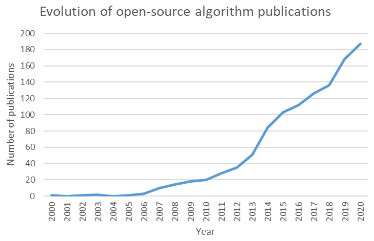
Figure 1 Evolution of yearly open-source algorithm publications between 2000 and 2020; data from Web Of Knowledge (last access: 1 September 2021).

An essential purpose of modelling is to support decision makers by offering a simplified representation of nature that also provides a corresponding quantitative assessment of uncertainty, communicating what we know, what remains unknown and what is ambiguous (Ferré, 2017). Uncertainty quantification is essential, because it allows mitigation of predictive uncertainty (Jessell et al., 2018) by expanding our knowledge, rejecting hypotheses (Wilcox, 2011) or falsifying scenarios (Raftery, 1993). Questions related to 3D geological modelling and uncertainty quantification are not just limited to the minerals industry, but also concern the fields of CO₂ sequestration (Mo et al., 2019), petroleum (Scheidt and Caers, 2009) and geothermal (Witter et al., 2019) energy resources as well as hydrogeology (Linde et al., 2017) or civil engineering in urban environments (Osenbrück et al., 2007; Tubau et al., 2017). Here, we are interested in the uses and practices of the minerals industry, that is dealing with both sedimentary basin and hard rock and/or cratonic settings across regional to mine scales.

The three main pillars of uncertainty quantification are the characterisation of uncertainty sources, their propagation and mitigation throughout the modelling workflow (see Fig. 2). The different sources of uncertainty, often overlooked, are related to measurement errors, interpretations, assumptions, modelling approximations and limited knowledge (sample size or unknown process). Measurement or data errors can be estimated by repetitive independent sampling or from instrument characteristics; they can be propagated through the modelling workflow by Monte Carlo data perturbation (Wellmann and Regenauer-Lieb, 2012; Lindsay et al., 2012; Pakyuz-Charrier et al., 2018). Combined with expert knowledge, initial datasets can be used to shape some assumptions and define plausible conceptual models but despite the importance of conceptual uncertainty on predictions (Pirot et al., 2015), it is too often limited to the definition of a unique scenario (Ferré, 2017). From a perspective on algorithms, some assumptions such as how to set parameter ranges are needed and this can greatly impact the definition of geological parameters (Lajaunie et al., 1997) prior to running predictive numerical simulations. Another aspect that is not always considered is the uncertainty related to a spatially limited sampling. Unsampled locations suggest a high uncertainty about the spatial distribution of the model parameters (or values of the property field); this is why it is preferable to resort to spatial stochastic simulations (e.g. sequential Gaussian simulations in a multi-Gaussian world) rather than interpolations (e.g. kriging) to generate models that are parameter fields (Journel and Huijbregts, 1978).

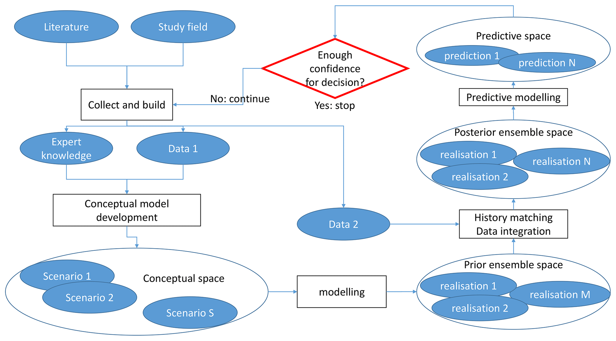
Figure 2 Schematic representation of a geomodelling workflow; each ellipse is associated with some uncertainty; Data 1 (e.g. geological observations) is used only to build a prior ensemble of models; Data 2 (e.g. geophysical measurements) is used to reduce the number of models that can be considered. It is achieved by exploring the ensemble of prior models and selecting those that are more likely to reproduce Data 2 within a prescribed level of error.

While the main objective of uncertainty quantification and data integration might be to improve the confidence level of predictions for decision making, it usually involves the generation of model ensembles via a Monte Carlo algorithm and it is rarely a straightforward step. Indeed, because of the high dimensionality and non-linearity of earth processes or the lack of data, history matching might prove difficult to achieve and predicted outcomes might present multiple modes (e.g. Suzuki and Caers, 2008; Sambridge, 2014; Pirot et al., 2017). In such cases, geological uncertainty analysis allows to improve our understanding of geological model (dis)similarities and how specific or shared features can be related to upstream parameters and downstream predictions. Model comparison requires a shared discrete support; one possibility is to project each geological model onto a discrete mesh such as a regular grid voxet composed of volumetric cells, also called voxels. Local uncertainty indicators such as voxel-wise entropy or cardinality (Lindsay et al., 2012; Schweizer et al., 2017), computed over an ensemble of geological voxets will inform about property field variability at specific locations (voxels) of the model mesh. Global indicators or summary metrics might be useful to identify how the statistics of specific patterns (e.g. fault or fracture network density, anisotropy, connectivity, etc.) evolve between different models and might also be a way to perform model or scenario selection (e.g. Pirot et al., 2019) or to reduce the dimensionality of the sampling space, from a high dimensional geological space to a low dimensional latent space (Lochbühler et al., 2013). Although some indicators have been used or developed for specific studies or softwares (Li et al., 2014), to the best of our knowledge, no independent uncertainty analysis tool applicable to both discrete and continuous property fields, combining local and global indicators is available to practitioners.

To investigate the uses and practices of the minerals industry regarding modelling and uncertainty quantification, we recently conducted a survey among numerical modelling practitioners from industry, government and academia in the sector of exploration and production of economic minerals. In this paper, first we present the main results and interpretations from this survey, the questions of which are listed in Appendix A. Second, to answer some of these needs, we propose a set of indicators to quantify geological uncertainty over an ensemble of geological models, represented as regular grid voxets and characterised by lithological units in the discrete domain and their underlying scalar field derived from implicit modelling in the continuous domain. The various indicators are illustrated with a synthetic case derived from a simplified Precambrian dataset of the Hamersley, Western Australia. The Python code called loopUI-0.1 (Pirot, 2021a) and the notebooks used to compute and illustrate these indicators are available at https://doi.org/10.5281/zenodo.5656151.

2 Survey

2.1 Material and method

The survey was designed to be concise to encourage participation but with several open-ended questions to maximise our chance to learn about different uses and practices, as well as to minimise induced bias whenever possible. The survey was in two parts. The first part was general and enquired about the scales and dimensions (questions 1 and 2) of geological models. The second part of the survey was more specific at a fixed modelling scale. It enquired about outputs or objectives (questions 3 and 4), about data input (question 5), current workflows (questions 6–9) and limitations and expected improvements (question 10).

It was distributed between October 2019 and January 2020 among the 3D Interest Group (3DIG, last access: 8 June 2022; https://www.linkedin.com/groups/6804787/members/, last access: 8 June 2022), Centre for Exploration Targeting (CET (last access: 8 June 2022) members (https://www.cet.edu.au/personnel/, last access: 8 June 2022; https://www.cet.edu.au/members/), Loop, last access: 8 June 2022; researchers (https://loop3d.github.io/loopers.html, last access: 8 June 2022) and related networks. About 150 persons were given the opportunity to participate. The solicited participants were essentially based in Australia but from a number of nationalities, with interests in geological modelling for mining applications. They were either from the industry or academia, from junior to senior profiles. Respondents had the opportunity to complete the survey on paper, in a text file or online.

A total of 35 responses were collected and anonymised. Of the responses seven concerned models at different scales, and when the second part of the survey was not clearly duplicated for each scale, the answers were considered with caution for each modelling scale. Although 35 responses is a relatively small number disallowing computation of robust statistics, statistical analysis was not the intended outcome. We endeavoured to ascertain opinions from practitioners in a specialised and important domain in the geosciences. The value is in the opinions we gathered which enhanced the survey results, aided interpretation and indicated which practices are commonly employed in geomodelling.

2.2 Results

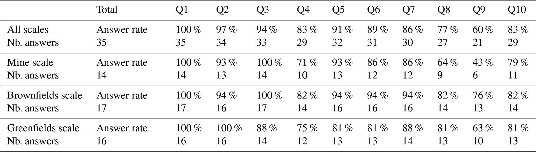
This section summarises the answers provided by the survey respondents. Table 1 provides the general statistics of answers to the survey. The high answer rate (mostly over 80 %) indicates that questions are meaningful for the respondents and indicates that the reader can have confidence in the presented results. The most answered question was Q1, about the modelling scale. The least answered question was Q9, about data integration and upscaling . The second least answered question was Q8, about the modelling workflow used. All other questions had an answer rate above 80 % on a global average. Note that the global number of survey answers was smaller than the sum of each survey answer grouped by scale, as some survey answers were returned only once for multiple scales.

Table 1 Global number and rate of answers per question and detailed by modelling scale.

Due to existing overlap of collected answers on different questions, the results presented hereafter summarise and group the collected answers by theme (output or objectives, input data, current modelling workflow and limitations), as outlined in the survey (see Appendix). Each theme is treated by modelling scale (see Fig. 3) when it involves different answers.

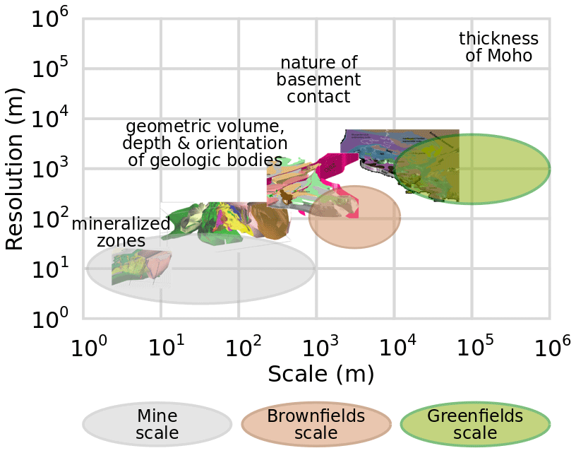
Figure 3 Modelling scales and resolutions in the mineral industry with examples of scale-specific scientific enquiry; model illustrations of the Vihanti-Pyhäsalmi Area, Finland, adapted from Laine et al. (2015).

Q3–4. The main modelling objectives depend on the scale of investigation. At the largest scales, investigation and modelling are particularly useful to assist exploration and prospectivity mapping. At the Greenfields or regional scale (>10 km dimension, ∼ 1 km resolution) , the main objective is to obtain a contextual and conceptual understanding of the regional geology, in particular regarding stratigraphy, topology and geochronology. At the Brownfields scale (1–10 km dimension, ∼ 100 m resolution), modelling aims to estimate deep structures beyond the depths reached by drilling, such as the depth of a particular interface or the delineation of potential mineral system components (e.g. fluid alteration pathways and ore deposition environments). At the Mine scale (<1 km dimension, ∼ 10 m resolution), the objectives are to assist with near mine exploration, resource estimation, ore body localisation, drill targeting, operation scheduling and efficient mining, by characterising local structures and geometries of stratigraphy and mineralisation. In addition to fulfilling these various objectives, 3D models are useful to improve hydrogeological characterisation, to identify critical zones where more knowledge has to be gained, to allow for comparison between datasets and test internal consistency, scenarios and last but not least, for visualisation and communication.

Q5. Data types used as input for geoscientific modelling are similar and complementary across scales. For instance, geological mapping, geophysical data (gravity, magnetics, electromagnetics, seismic), and geochemistry are useful at all scales even though the related measurements might inform about a regional trend. Drill hole-derived data are usually much more abundant at the Mine scale and can be useful to understand the regional context if analysed with this alternative use in mind. For example, drill logs that only record the presence or absence of mineralisation are not useful for the regional context; however, those that record rock properties, lithology and structure can be extrapolated to larger scales and integrated in regional models (e.g. Lindsay et al., 2020).

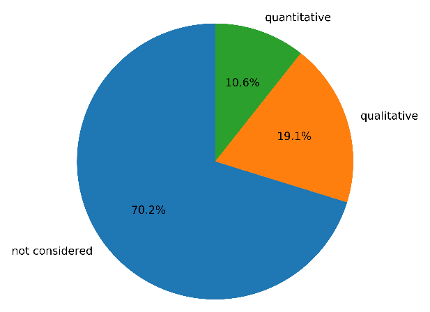
Q6. Regarding current modelling practices, although the survey respondents acknowledge the importance of uncertainty quantification and propagation into modelling to estimate the confidence around predictions, only about 10 % perform quantitative uncertainty characterisation and propagation from input data; about 20 % do some qualitative characterisation and a vast majority of 70 % recognise that it is ignored (see Fig. 4).

Figure 4 Consideration of input data uncertainty in modelling.

Q7–9. Modelling steps, assumptions or geological interpretations are not recorded in one third of the cases. In most cases, assumptions and elements of the modelling process are described in metadata or in separate reports. In very few cases, specific procedures and tools are available to keep track of these. The respondents use a variety of software, platforms or programming tools to produce 3D geological models and further data integration. The lack of a coherent workflow introduces the potential for uncertainty, error and loss of precision when forced to translate data formats across multiple software platforms, in addition to the time lost that could otherwise be dedicated to solving the problem under question or exploring alternative hypotheses.

Q10. Overall, the main limitations involved in 3D geological modelling are uncertainty underestimation due to strong constraining and underlying assumptions (e.g. lack of consideration of alternative conceptual models, lack of uncertainty around interpreted horizons), navigation between scales, the amount of work required to process and prepare input data (including necessary artificial data), the time required to generate one model, the difficulty to integrate 2D data into a 3D framework, the difficulty to visualise and manage huge amounts of drill hole data in 3D, the advent of geological inconsistencies, workflow and model reproducibility given the same inputs, joint integration of geological and geophysical data and lack of tools to visualise uncertainty.

In what follows we address one of the needs identified in the survey: the lack of tools to quantify and visualise uncertainty from an ensemble of 3D voxets (prior or posterior ensembles). Indeed, it is of utmost importance for practitioners as it allows reinterpretation of data or scenario importance with respect to geological uncertainty or predictive uncertainty.

3 Uncertainty indicators for categorical or continuous property fields

The estimation of prediction confidence in geosciences relies heavily on numerical simulations and requires generation of an ensemble of models. As indicated by the survey results, an important aspect of uncertainty quantification is its representation. It helps identifying specific features or zones of interest. Moreover, respondents estimate that such visualisation tools are missing. The uncertainty indicators presented hereafter provide a way to identify zones of greater or smaller uncertainty as well as (dis)similarities between geomodel realisations.

Geomodels can be used to convey very different discrete or continuous properties. Discrete or categorical properties, such as lithological formations or classification codes should be compared carefully. Indeed, while it is straightforward to state if two values are identical or different, additional information is needed to rank dissimilarities. Continuous properties, such as potential fields or physical properties (e.g. porosity, conductivity) do not present this ambiguity to compare range of values. One can note that depending on how physical properties are assigned during modelling, their value spectrum might be discrete. Some modelling platforms may produce a discrete physical property value spectrum depending on how physical properties are assigned or what input constraints are enforced during model construction.

Local measures of uncertainty provide indicator voxets of the same dimensions as the voxets of a model ensemble. For a given voxel, uncertainty indicators are computed from the distributions of values taken by a given property at the corresponding voxel (same location) across the ensemble of model realisations. Such local indicators are very convenient for visualisation: by sharing the same voxet as the model realisations, it is relatively easy to spot zones of low or high uncertainty. However, to be useful it requires advanced modelling that integrates some spatial constraints and possibly computationally expensive, particularly if they are produced by inversion algorithms. Here, we propose to compute cardinality and Shannon's entropy for discrete properties (e.g. Wellmann and Regenauer-Lieb, 2012; Pakyuz-Charrier et al., 2018), and similarly, range, standard deviation and continuous entropy for continuous properties (e.g. Marsh, 2013; Pirot et al., 2017).

Global measures rely on the computation of summary statistics or on the identification of feature characteristics, independently from their locations. The dissimilarities between summary statistics or characteristics can be estimated via appropriate metrics, such as the Wasserstein distance (Vallender, 1974) or the Jensen-Shannon divergence (Dagan et al., 1997). The resulting global measures allow comparison of models with voxets or meshes of different dimensions. However, the computation of summary statistics might be more time consuming than local measures. Their main advantage is that it enables a focus on pattern similarity between models which might be particularly useful to explore the selection of alternative scenarios or prior realisations, before data integration and history matching. In what follows, we propose a series of dissimilarity measures, applicable to categorical and continuous property fields, based on 1-point statistics (histogram, Dagan et al., 1997), 2-point (geo)statistics (semi-variogram, Matheron, 1963), multiple-point statistics (multiple-point histogram, Boisvert et al., 2010), connectivity (Renard and Allard, 2013), wavelet decomposition (e.g. Scheidt et al., 2015) and topology (e.g. Thiele et al., 2016). Some indicators are similar to exploratory data analysis techniques but here they are applied to model ensemble analysis.

To illustrate the different indicators, inspired by a Precambrian geological setting, that is a simplified dataset from the Hamersley region, Western Australia, we generated synthetic ensembles of 10 model sets for 3 different scenarios. Each model set is composed of a lithocode voxet describing the lithological units (categorical variable), and of its underlying scalar field voxet (continuous variable). The underlying scalar field is obtained by composition of the different scalar fields for each unconformable stratigraphic group. Scenario 1 considers all synthetic input data, while scenario 2 keeps only 50 % of the data within a north-south limited band and scenario 3 retains input data with a 50 % probability (see Fig. 5). For each scenario, the positions and orientations of the input data are perturbed to provide 10 stochastic realisations. Positions are perturbed with a Gaussian error of zero mean and 3 m standard deviation. Orientations are perturbed with a von Mises-Fisher error of κ=150 (corresponding to about $\pm \mathrm{5}{}^{\circ }$ of error). Each 3D model was generated using LoopStructural (Grose et al., 2021).

Figure 5 Example model set of lithocode and scalar fields for each of the three scenarios; the left column illustrates input data and model set for scenario 1 when all data are considered; the middle column illustrates input data and model set for scenario 2 when 50 % of the data within a band are considered; the right column illustrates input data and model set for scenario 3 where each input data are decimated with a probability of 50 %.

3.1 Cardinality

The cardinality of a set in mathematics, is the number of elements of the set. Here, we define the cardinality for a given voxel as the number of unique elements over the ensemble of models for the corresponding voxel (Lindsay et al., 2012). Computed for all voxels, it provides a cardinality voxet of the same dimensions as the model voxets. It assumes that all voxets of the model ensemble have the same dimensions. By definition, this indicator can be computed on discrete or categorical property fields. For continuous property fields, we propose to use the range between the minimum and maximum value, the standard deviation. Eventually, these continuous indicators can be normalised over the voxet and then averaged or weighted to provide another indicator. Figure 6 shows a cardinality voxet computed from an ensemble of lithocode voxets as well as the range, standard deviation and their normalised average from an ensemble of density voxets.

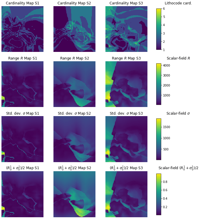
Figure 6 Horizontal sections of cardinality voxets for a categorical property field (first row) or similar indicators for a continuous property field (second–fourth row); the first row shows the cardinality over the ensemble of lithocode voxets, the second row displays the (max-min range) over the ensemble of scalar field voxets, the third row presents the standard deviation over the ensemble of scalar field voxets, the fourth row displays the averaged normalised range and standard deviation over the ensemble of scalar field voxets; the left column refers to scenario 1, the middle column to scenario 2 and the right column to scenario 3.

3.2 Entropy

Shannon's entropy (see Eq. 1) is a specific case of the Rényi entropy when its parameter α converges to 1 (Rényi, 1961). It has been already been applied to geomodels for a few decades (Journel and Deutsch, 1993; Wellmann and Regenauer-Lieb, 2012) and is a finer way than cardinality to describe uncertainty over an ensemble of models, as it takes into account the histogram proportions of the unique values encountered. Let us consider the categorical or discrete variable X that represents a voxel property and assume that it can take n distinct values among an ensemble of voxets. By denoting the probability of observing the ith possible value as p_i, the entropy H of X is computed as follows:

$$\begin{array}{}\text{(1)}& H\left(X\right)=-\sum _{i=\mathrm{1}}^n{p}_i\ln p_i.\end{array}$$

For continuous property fields, one needs to discretise the continuous domain and integrate along the width of the bins (Marsh, 2013). Here, for the considered example, we choose 50 regular bins. Figure 7 displays Shannon's entropy for the lithocode voxets and the continuous entropy for the other ensemble of property fields: magnetic field, gravity field, density and magnetic susceptibility.

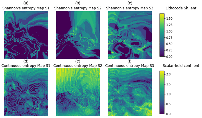
Figure 7 Horizontal sections entropy voxets; (a–c) show Shannon's entropy over the ensemble of lithocode voxets, (d–f) display the continuous entropy over the ensemble of scalar field voxets; (a) and (d) refer to scenario 1, (b) and (e) to scenario 2 and (c) and (f) to scenario 3.

3.3 Histogram dissimilarity

Given a pair of voxets V_P and V_Q, we measure the dissimilarities between their histograms by computing a symmetrised and smooth version of the Kullback-Leibler divergence (Kullback and Leibler, 1951) known as the Jensen-Shannon divergence or total divergence to the average (Dagan et al., 1997). Given two random variables P and Q, the Jensen-Shannon divergence is computed as JSD$\left(P\right|\left|Q\right)=\frac{\mathrm{1}}{\mathrm{2}}$KLD$\left(P\right|\left|M\right)+\frac{\mathrm{1}}{\mathrm{2}}$KLD$\left(Q\right|\left|M\right)$, where $M=\frac{P+Q}{\mathrm{2}}$ and KLD is the Kullback-Leibler divergence. It requires P and Q to share the same support 𝒳 and can be computed for continuous or discrete variables. Here, we assume that for our pair of voxets V_P and V_Q, the support of our random variables P and Q, respectively, is discrete and of size n (possibly n bins for discretised continuous variables).

Denoting the support of P and Q by (x_i)_i=1…n, $p_i=\text{Prob}(P=x_i)$, $q_i=\text{Prob}(Q=x_i)$ and $m_i=\frac{p_i+q_i}{\mathrm{2}}$, the Jensen-Shannon divergence is computed as in Eq. 2.

$$\begin{array}{}\text{(2)}& \mathrm{JSD}\left(P\right|\left|Q\right)={\displaystyle \frac{\mathrm{1}}{\mathrm{2}}}\sum _{i=\mathrm{1}}^n{p}_i\ln \left({\displaystyle \frac{p_i}{m_i}}\right)+{\displaystyle \frac{\mathrm{1}}{\mathrm{2}}}\sum _{i=\mathrm{1}}^n{q}_i\ln \left({\displaystyle \frac{q_i}{m_i}}\right).\end{array}$$

3.4 Semi-variogram dissimilarity

Introduced by Matheron (1963), the semi-variogram measures the dissimilarity of values taken by random variables at different spatial locations as a function of distance. Assuming stationarity, it can be written as

$$\mathit{\gamma }\left(\mathit{h}\right)={\displaystyle \frac{\mathrm{1}}{\mathrm{2}}}E\left[{\left(Z\left(\mathit{s}\right)-Z(\mathit{s}+\mathit{h})\right)}^{\mathrm{2}}\right],$$

where s​​​​​​​ denotes a spatial location vector, h denotes a vector and Z is the random field of interest.

Using spatial samples of a random variable, and segmenting the h space into radial distance lags, it is then possible to compute an experimental or empirical semi-variogram over n lags of width δ as follows:

$$\widehat{\mathit{\gamma }}\left(h_i\right)={\displaystyle \frac{\mathrm{1}}{\mathrm{2}{N}_i}}\sum _{(j,k)}\left|Z\right({\mathit{s}}_j)-Z({\mathit{s}}_k){|}^{\mathrm{2}},$$

where $h_i=(i-\frac{\mathrm{1}}{\mathrm{2}})\mathit{\delta }$ is the centre of the ith lag, $\mathrm{1}\le i\le n$ and N_i is the number of pairs (j,k) of points such that $(i-\mathrm{1})\mathit{\delta }\le \left|\right|{\mathit{s}}_j-{\mathit{s}}_k\left|\right|\le i\mathit{\delta }$. Note, that we obtain here an omnidirectional semi-variogram; it will be less sensitive to anisotropy but simpler to assess than many directional semi-variograms as anisotropic directions.

Given two empirical semi-variograms $\widehat{{\mathit{\gamma }}_{\mathrm{1}}}$ and $\widehat{{\mathit{\gamma }}_{\mathrm{2}}}$ (see e.g. Fig. 8), we propose to use a weighted l_p norm as defined in Eq. (3).

$$\begin{array}{}\text{(3)}& \left|\right|\widehat{{\mathit{\gamma }}_{\mathrm{1}}}-\widehat{{\mathit{\gamma }}_{\mathrm{2}}}|{|}_p={\left({\displaystyle \frac{\mathrm{1}}{\sum _{\mathrm{1}\le i\le n}\frac{\mathrm{1}}{h_i}}}\sum _{\mathrm{1}\le i\le n}{\displaystyle \frac{\mathrm{1}}{h_i}}\left|\widehat{{\mathit{\gamma }}_{\mathrm{1}}}\right(h_i)-\widehat{{\mathit{\gamma }}_{\mathrm{2}}}(h_i){|}^p\right)}^{\frac{\mathrm{1}}{p}},\end{array}$$

where p=2 in the following examples. Note that the weight is inversely proportional to the lag distance, giving more importance to dissimilarities of the semi-variogram for small distances. This allows to account for the structural noise and (dis)continuity of the property fields. Thus, the experimental semi-variogram is not always well-behaved at short distances, in particular when dealing with sparse data. However, this is not a concern when considering fully populated voxets, such as in our case.

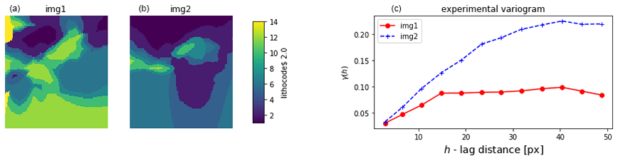
Figure 8 Example of experimental semi-variogram for two lithocode voxets, computed for the lithocode value of 2; (a) and (b) show a horizontal section for each voxet; (c) shows the two corresponding experimental semi-variogram.

3.5 Connectivity dissimilarity

The existence of preferential flow-paths or barriers in the subsurface often has a strong impact in many geoapplications. Their characterisation can improve the management of groundwater quality, the extraction of geothermal energy, and help mitigate the environmental impact related to either the production of non-renewable and renewable resources from the subsurface or the sequestration of carbon dioxide and waste (e.g nuclear waste). Renard and Allard (2013) have shown that connectivity cannot be captured by topological indicators, such as the Euler characteristic, or by 1-point or 2-point statistics (e.g. by histogram or semi-variogram analysis, respectively). However, they have shown how a global percolation metric Γ(p) and a lag distance connectivity function τ(h) are useful to characterise the connectivity of binary, categorical or continuous property fields. Connectivity indicators have also been used in multiple-point statistics applications to characterise the quality of stochastic simulations with respect to a training image (Meerschman et al., 2013) and in hydrogeophysical application for model selection (Pirot et al., 2019).

Let us consider a binary spatial variable $X\in \mathrm{0},\mathrm{1}$, and a distance h. Then, the lag distance connectivity function τ(h) is defined as the probability that two h-distant points s and s+h, whose value of X=1, are connected. For a binary voxet, two voxels are connected if a path through the face of successive neighbour voxels with the same property exists. The lag distance connectivity function (see Fig. 9) can be written as

$$\mathit{\tau }\left(\mathit{h}\right)=\mathrm{Prob}\left(\mathit{s}\stackrel{\mathrm{connected}}{\leftrightarrow }\mathit{s}+\mathit{h}\left|X\right(\mathit{s})=\mathrm{1},X(\mathit{s}+\mathit{h})=\mathrm{1}\right).$$

Figure 9 Illustration of the τ(h) connectivity function (b) computed on a 2D horizontal section from a binary 3D voxet (a).

Now let us assume that the percolation threshold p produces a binary voxet characterised by the binary spatial variable $X\in \mathrm{0},\mathrm{1}$. The global percolation metric Γ(p) (see Fig. 10) is the proportion of the pairs of voxels that are connected amongst all the pairs of voxels for which X=1:

$$\mathrm{\Gamma }\left(p\right)={\displaystyle \frac{\mathrm{1}}{n_p^{\mathrm{2}}}}\sum _{i=\mathrm{1}}^{N\left(X_p\right)}{n}_i^{\mathrm{2}}=\sum _{i=\mathrm{1}}^{N\left(X_p\right)}{p}_i^{\mathrm{2}},$$

where N(X_p) is the number of distinct connected components formed by voxels of value X=1 and $p_i=n_i/n_p$ is the proportion of voxels forming the ith distinct connected component, n_i being the size in voxels of the ith connected component and n_p being the total number of voxels of value X=1 in the voxet.

Figure 10 Illustration of a scalar field voxet horizontal section (a) and its global percolation metrics Γ(p) and Γ^c(p) (b) computed over the 2D sections; (c–g) display horizontal sections of binary fields obtained by applying different percolation threshold p[%] to the scalar field 3D voxet; blue areas, above the percolation threshold, contribute to Γ(p); yellow areas, below the percolation threshold, are used to compute Γ^c(p).

Conversely, for the complementary set of voxels for which X=0, we can compute Γ(p)^c (see Fig. 10). One can note that the two connectivity metrics are related as $\sum _h\mathit{\tau }\left(\mathit{h}\right)=n_p\mathrm{\Gamma }\left(p\right)$ (Renard and Allard, 2013).

We propose two measures of connectivity dissimilarity between voxets, based either on τ(h) or Γ(p) and Γ(p)^c. Let us denote by N_c the number of considered classes of values. Note that for a categorical variable voxet, the classes are defined by the category values, while for continuous variable voxet, they can be obtained by thresholding with N_c percolation thresholds p. Let us consider N_lag the number of lags (defined similarly as for the experimental semi-variogram in the previous subsection), l_p=2 the distance norm and ${\text{𝟙}}_{\mathit{\tau }}=\mathrm{1}-{\text{𝟙}}_{\mathrm{\Gamma }}$ the indicator allowing to choose between τ or Γ connectivity. Then we can compute the connectivity dissimilarity between two voxets as follows in Eq. (4):

$$\begin{array}{}\text{(4)}& \begin{array}{rl}& d_{\text{CTY}}({\text{Voxet}}_{\mathrm{1}},{\text{Voxet}}_{\mathrm{2}})=\sum _{i=\mathrm{1}}^{N_{\mathrm{c}}}{\displaystyle \frac{\mathrm{1}}{N_{\mathrm{c}}}}\\ & \left[{\text{𝟙}}_{\mathit{\tau }}\left(\sum _{\mathit{h}=\mathrm{1}}^{N_{\mathrm{lag}}}{\displaystyle \frac{\left|{\mathit{\tau }}_{\mathrm{1}}\right(\mathit{h})-{\mathit{\tau }}_{\mathrm{2}}(\mathit{h}){|}^{l_p}}{N_{\mathrm{lag}}}}\right)+(\mathrm{1}-{\text{𝟙}}_{\mathit{\tau }})\left|{\mathrm{\Gamma }}_{\mathrm{1}}\right(i)-{\mathrm{\Gamma }}_{\mathrm{2}}(i){|}^{l_p}\right].\end{array}\end{array}$$

3.6 Multiple-point histogram dissimilarity

Multiple-point histograms (MPH, Boisvert et al., 2010) are based on pattern recognition and have been primarily used in the field of geostatistics (Guardiano and Srivastava, 1993) to quantify the quality of multiple-point statistics simulations. Patterns are delimited by a search window whose dimensionality matches the one of the dataset. One can count unique patterns; however, the number of unique patterns might be relatively important, in particular for continuous property fields. In that case, it might require that the analysis be restrained to the most frequent patterns (Meerschman et al., 2013). An alternative is to base the analysis on pattern cluster representatives (see Fig. 11). Here, using an l₂ norm distance between patterns and k-means clustering (Pedregosa et al., 2011, scikit-learn implementation), we classify all patterns into N_c=10 clusters. Each cluster centroid or barycentre defines its representative.

Figure 11 Illustration of multiple-point histogram cluster representatives and sizes for two scalar field horizontal sections, at the 3rd upscaling level; the left column shows the two 2D voxets; for the other columns the first and second rows, and the third and fourth rows, display the 10 cluster representatives and their size (number of counted patterns attached to the cluster representative) for the first voxet and for the second voxet, respectively; their order reflects the best similarity between the cluster representatives for both voxets.

In addition, voxets can be easily upscaled, which allows MPH analysis of potentially large scale features with a small search window at a high level of upscaling. Note that at a given level l of upscaling, the size of the dataset is divided by 2^l along each dimension. Here, to avoid property values smoothing, we perform a stochastic upscaling, i.e. in a 2D case, the upscaled value of a 2×2 subset of pixels is achieved by a uniform random draw among the values of the 4 pixels. Cluster pattern identification is performed at the initial resolution level (l=0) and at all possible upscaled levels.

For a given upscaling level, once k-means clustering of patterns has been performed on two voxets or datasets, distances between cluster representatives of two images can be computed

$$d(C_{\mathrm{1}}^i,C_{\mathrm{2}}^j)={\left(\sum _{w=\mathrm{1}}^{N_{\mathrm{w}}}{\left(C_{\mathrm{1}}^i\left(w\right)-C_{\mathrm{2}}^j\left(w\right)\right)}^{\mathrm{2}}\right)}^{\frac{\mathrm{1}}{\mathrm{2}}},$$

where $C_{\mathrm{1}}^i$ is the ith cluster representative for voxet 1, $C_{\mathrm{2}}^j$ is the jth cluster representative for voxet 2 and w denotes the index of the window search elements.

The cluster representatives between two datasets are paired by similarity (smallest distance), and reordered such that ∀i, $\mathrm{1}\le i\le N_{\mathrm{c}}$, and $C_{\mathrm{1}}^i$ is paired with $C_{\mathrm{2}}^i$. To account for cluster size differences, the distance between paired cluster representative are weighted by proportion dissimilarities. It results in an MPH cluster-based distance between voxets or datasets 1 & 2 defined as in Eq. (5).

$$\begin{array}{}\text{(5)}& \begin{array}{rl}& d_{\mathrm{MPH}}({\mathrm{Voxet}}_{\mathrm{1}},{\mathrm{Voxet}}_{\mathrm{2}})=\sum _{i=\mathrm{1}}^{N_{\mathrm{c}}}{\displaystyle \frac{\mathrm{1}}{N_{\mathrm{c}}}}\\ & \left[\left(\mathrm{1}+d(C_{\mathrm{1}}^i,C_{\mathrm{2}}^i)\right)\times \left(\mathrm{1}+{\displaystyle \frac{|p_{\mathrm{1}}^i-p_{\mathrm{2}}^i|}{p_{\mathrm{1}}^i+p_{\mathrm{2}}^i}}\right)-\mathrm{1}\right],\end{array}\end{array}$$

where $p_{\mathrm{1}}^i$ and $p_{\mathrm{2}}^i$ are the proportions of the paired clusters $C_{\mathrm{1}}^i$ and $C_{\mathrm{2}}^i$ with respect to voxets 1 & 2, respectively.

One advantage of selecting cluster representatives independently between two voxets is to lower computing requirements over large ensembles of voxets, performing the analysis for N_v voxets instead of $\frac{N_{\mathrm{v}}(N_{\mathrm{v}}-\mathrm{1})}{\mathrm{2}}$ pairs. However, performing R pattern clustering on two datasets might provide a more accurate and precise way to compute a distance between histograms with the same support of cluster representatives, thus allowing the use of Jensen-Shannon divergence for instance. One can note that we accounted for the size of the clusters but we could also consider the density spread or concentration around cluster representatives.

3.7 Wavelet decomposition coefficient dissimilarity

Wavelet decomposition is a way to compress images. Each level of decomposition produces a series of coefficients. If computed for images to be compared, the dissimilarity of histograms of coefficients can be computed with the Jensen-Shannon divergence (Eq. 2). Here, wavelet decomposition (Fig. 12) is performed with the PyWavelets Python package (Lee et al., 2019) at all possible levels of decomposition and using the “Haar” wavelet. Other wavelets could be used; however, tests have shown that such dissimilarity measures are not very sensitive to the choice of the wavelet (Pirot et al., 2019).

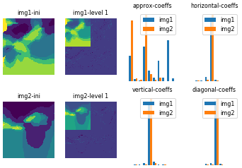
Figure 12 Illustration of a first level of Haar-wavelet decomposition and the resulting coefficient histograms for two lithocode voxet horizontal sections.

Then a wavelet-based dissimilarity measure between two voxet can be computed as in Eq. (6) by summing the Jensen-Shannon divergences computed for all pairs of approximation and decomposition coefficients at all possible levels:

$$\begin{array}{}\text{(6)}& d_{\mathrm{WVT}}({\mathrm{Voxet}}_{\mathrm{1}},{\mathrm{Voxet}}_{\mathrm{2}})=\sum _{i,j}{\displaystyle \frac{\mathrm{JSD}\left(C_{\mathrm{1}}^{i,j}\right|\left|C_{\mathrm{2}}^{i,j}\right)}{\sum _{i,j}\mathrm{1}}},\end{array}$$

where $C_{\mathrm{1}}^{i,j}$ and $C_{\mathrm{2}}^{i,j}$ denote the distributions of the ith coefficients at upscaling level j for Voxet₁ and Voxet₂, respectively.

3.8 Topological dissimilarity

Thiele et al. (2016) give an overview of possible representations of the topology in the context of 3D geological modelling. Different levels of complexity (e.g. 1st or 2nd orders…) can be used. Nonetheless, any topological indicator is a graph that can take the form of an adjacency matrix. Therefore, to compute a topological distance between two 3D geological models (for instance as in Giraud et al., 2019), it seems natural to look at distances defined between graphs. Donnat and Holmes (2018) provided a comprehensive review of graph distances used in the study of graph dynamics or temporal evolution. Although, here, in a geological context, we aim at comparing the topological diversity of an ensemble of geological models, we can use similar distances. Donnat and Holmes (2018) classified graph distances into three main categories as summarised below.

Low-scale distances capture local changes in the graph structure. The Hamming (structural) distance is the sum of the absolute value of differences between two adjacency matrices and requires the same number of vertices (nodes) between the graphs – note that it is a specific case of the more general graph edit distance. The Jaccard distance is defined as the difference between the union and intersection of two graphs. The graph edit distance belongs to the NP-complete class of problems, and is not computed here. More information is available in (Gao et al., 2010) or in part IV Chapter 15 of the Encyclopedia of Distances (Deza and Deza, 2009, p. 301). Note that some packages and implementations to compute the graph-edit distance exist but have not been tested here (GMatch4py, last access: 8 June 2022; graphkit-learn, last access: 8 June 2022; other proposed heuristic, last access: 8 June 2022).

High level or spectral distances are global measures and reflect the smoothness of the overall graph structure changes by measuring dissimilarities in the eigenvalues of the graph Laplacian or its adjacency matrix. Some examples are the IM distance (Ipsen and Mikhailov, 2003), l_p distances on eigenvalues and the Kruglov distance on eigenvector coordinates (Shimada et al., 2016).

Meso-scale distances are a compromise or combination of low-scale and spectral distances: Hamming-IM (HIM) combination, heat-wave distance, polynomial distance, neighbourhood level distances and connectivity-based distances.

Here, we propose to build first order adjacency matrices (see Fig. 13) from 2D or 3D voxet models. For continuous property fields, the voxet is discretised into N=10 classes of values defined by N equipercentile thresholds over the distribution of the combined voxets. We compute two topological distances: the structural Hamming distance and the Laplacian spectral distance (Shimada et al., 2016).

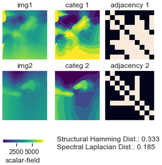
Figure 13 Illustration of topological distances and adjacency matrices in the right column for two categorised voxets in the middle column, derived from two scalar field voxet horizontal sections in the left column.

Note that graphs characterising geological model topology could be defined as attributed graphs, to contain more information (edges properties, such as age constraint, type of contact; vertices properties, such as formation type, geophysical properties). Thus, more specific measures could be developed to take such characteristics into account; however, it would rely on the ability of geomodelling engines to provide these topology graphs with each model, and there is no guarantee that it would be meaningful for the inference of geochronology from geophysics.

3.9 Results: indicator comparison

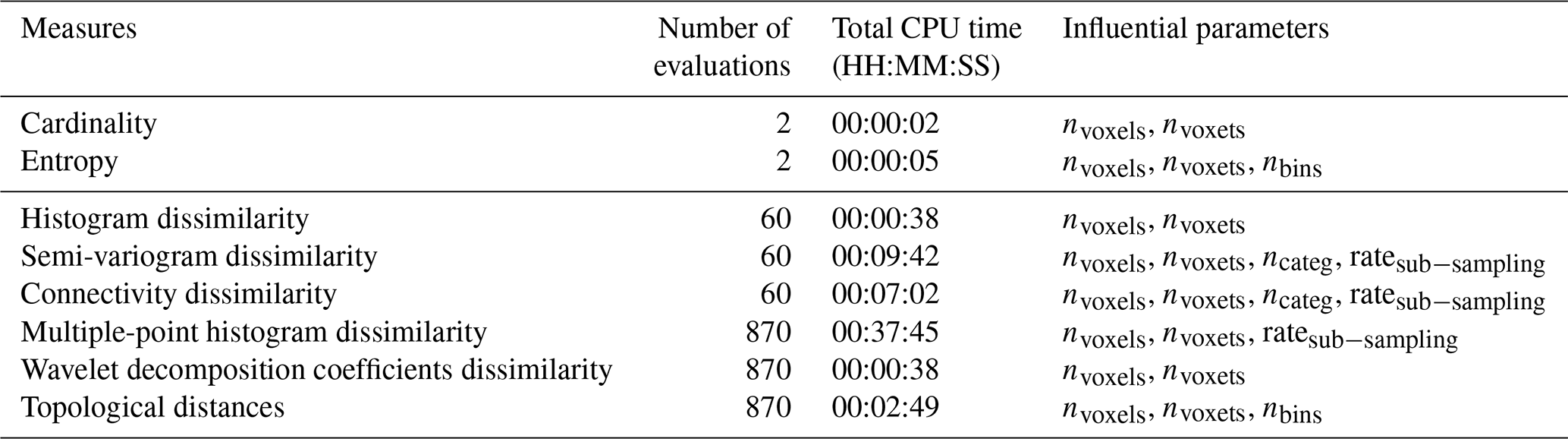
Local measures of uncertainty (see Figs. 14 and 15) and global indicators (see Figs. 17 and 18) have been computed for 2D, 3D, categorical and continuous variable voxets (lithocode, scalar field) for an ensemble of 30 model sets. We also provide a comparison of the required computing time for the different indicators and highlight the contributing factors or parameters (see Table 2).

One can see from Fig. 14 that Shannon's entropy and cardinality computed from lithocode voxets can have a good correlation. However, the following equivalent indicators: continuous entropy, averaged normalised range and standard deviation computed from scalar field voxets, (Fig. 15) have very little in common. Indeed, the standard deviation or the range of values is sensitive to extremely different values, while the continuous entropy is sensitive to the proportion of categories of values.

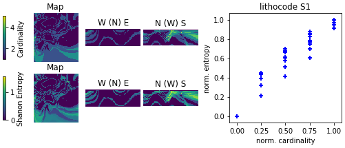
Figure 14 Comparison of local uncertainty measures for an ensemble of 10 lithocode 3D voxets for scenario 1; 3D visualisation looking from the NW of the voxet, the top surface of the voxet an EW section at the northern face of the model looking from the south, a NS section on the western face of the voxet looking from the east.

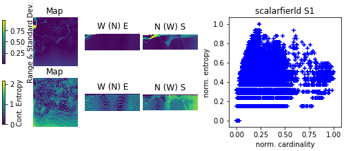
Figure 15 Comparison of local uncertainty measures for an ensemble of 10 scalar-field 3D voxets for scenario 1; 3D visualisation looking from the NW of the voxet, the top surface of the voxet an EW section at the northern face of the model looking from the south, a NS section on the western face of the voxet looking from the east.

Figure 16 shows that histogram dissimilarities computed from lithocode or scalar field voxets have a good correlation. Multidimensional scaling (MDS) plots reveal that dissimilarities are smallest within scenario 1 and then within scenario 3 while they are greatest within scenario 2. The MDS plots show that scenarios 1 and 3 model sets overlap while scenario 2 model sets are characterised by less similar histograms and thus the scenario 2 sample cloud of points form a distinct cluster.

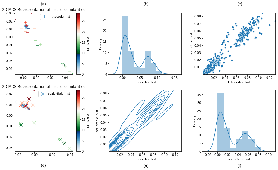
Figure 16 Comparison of model set histogram dissimilarities across the three scenarios; (a) and (d) display a 2D MDS representation of histogram dissimilarities computed from lithocode voxets (a–c) and from scalar-field voxets (d–f); samples 0–9 belong to scenario 1, samples 10–19 belong to scenario 2 and samples 20–29 belong to scenario 3; the subplots of (b), (c), (e), and (f) show histogram and density, joint density and cross-plot between histogram dissimilarities computed from lithocode voxets or from scalar field voxets.

Figure 17 shows some correlation between histogram, semi-variogram, wavelet and structural Hamming-based measures from the lithocode voxets. Figure 18 shows a good correlation between histogram dissimilarity, wavelet-based dissimilarity and structural Hamming distance from the scalar field voxets but not as strong as when computed from the lithocode voxets.

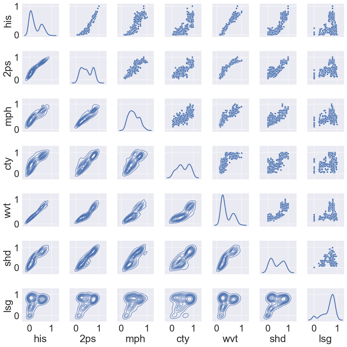
Figure 17 Comparison of global normalised dissimilarity measures for an ensemble of 30 lithocode 3D voxets across the 3 scenarios; cross-plots and density plots by pair of normalised dissimilarity measures; his – histogram, 2ps – semi-variogram, mph – multiple-point histogram, cty – connectivity, wvt – wavelet decomposition coefficients, shd – topological structural Hamming distance, lsg – topological Laplacian spectral distance.

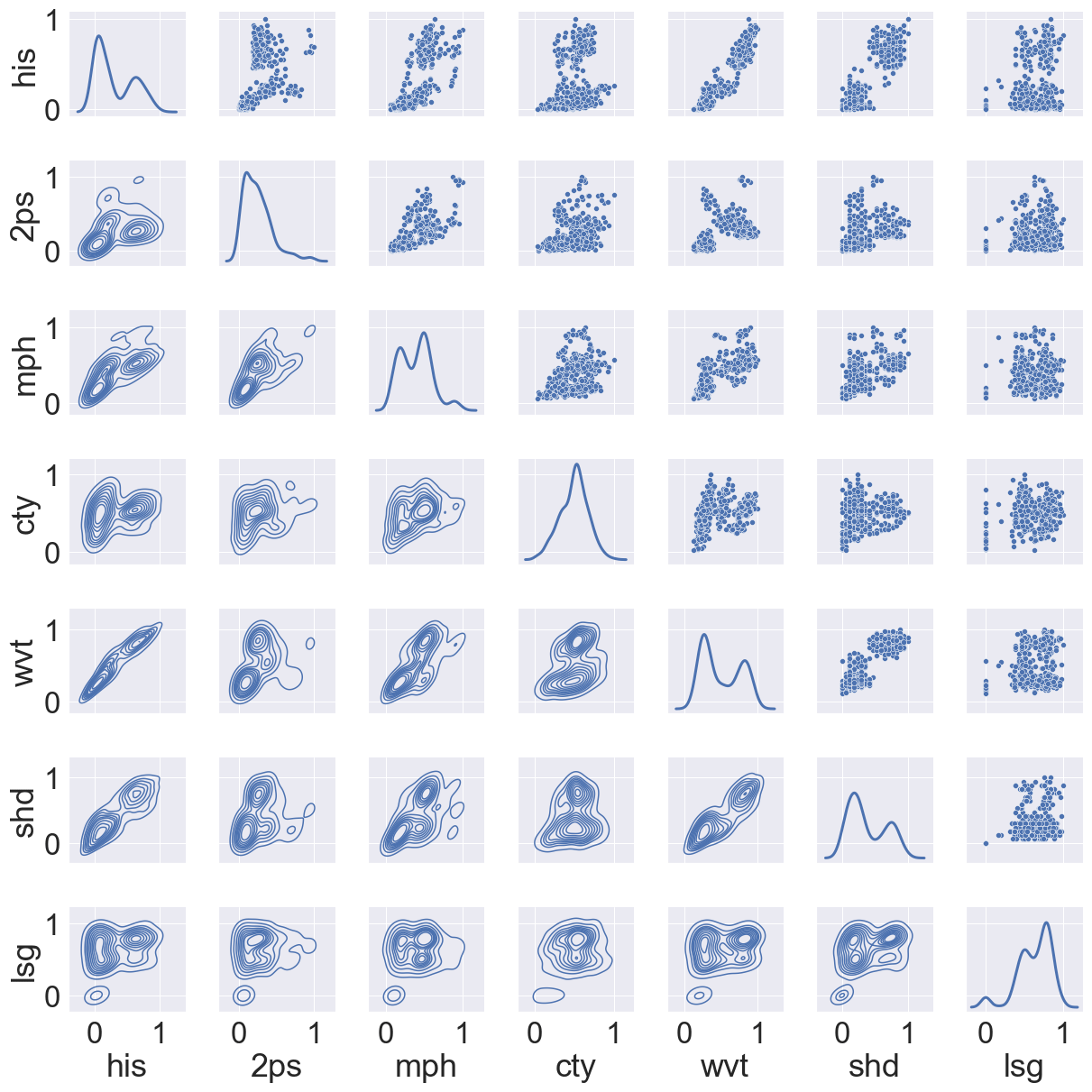
Figure 18 Comparison of global normalised dissimilarity measures for an ensemble of 30 scalar field 3D voxets across 3 scenarios; cross-plots and density plots by pairs of normalised dissimilarity measures; his – histogram, 2ps – semi-variogram, mph – multiple-point histogram, cty – connectivity, wvt – wavelet decomposition coefficients, shd – topological structural Hamming distance, lsg – topological Laplacian spectral distance.

Table 2 Complexity and computing time for local and global measures of uncertainty using a single Intel^®Core™ i7-8550 1.80 GHz processor, based on an ensemble size of N=10 geological models.

4 Discussion

Several factors might explain why the majority of practitioners do not consider input data uncertainty but all are related to the limited resources available to practitioners (knowledge, algorithms, computing time, project timeframe or funding). One of them is that data uncertainty is not quantified at the time of data acquisition or not available for some measurements, which is the case when only one measurement or observation of geological data is made at a given location (e.g. for azimuth, dip, and lithology). Reasonable metadata standards may help to enforce error quantification, or at the very least provide some information about the nature of data collection as to infer where and what magnitude of error may be present but even these are poorly or not recorded. Although repeated independent measurements would provide uncertainty estimates, procedures and limited time or budget resources are a hindrance. Sometimes, knowing the survey set-up and the instrumentation characteristics, such as their precision and accuracy might avoid repeating field measures and allow an estimation of measurement uncertainty. Inversion algorithms used for geophysical data integration can also provide estimates of geophysical data errors.

A second reason is related to the required time and associated costs of modelling. Indeed, the process of data integration only uses a very limited amount of automation, thus the generation of a single model already consumes most of the practitioners’ resources. In addition, the complexity of real-world data often leads to a substantial number of parameters. Thus for high-dimensional problems, uncertainty propagation requires sufficiently large model ensembles to be representative, which might not be compatible with the limited resources available to the practitioners.

A third reason is due to the fact that assumptions, such as choices in geological interpretations made during the modelling process, are not always tracked and when they are, they are often “forgotten” at the next stage of the modelling workflow (Jessell et al., 2018). When these assumptions or justifications are recorded, they are described in metadata or in distinct reports. Consequently, conceptual uncertainty, which describes alternative yet plausible stratigraphy, tectonic and geodynamic settings, is also ignored.

Another possible reason is that uncertainty is ignored out of convenience (Ferré, 2017) or by ignorance, lack of knowledge or education about the importance of uncertainty quantification. However, the formulation of the collected answers suggests that this is not the case for the surveyed practitioners, who tend to acknowledge the importance and need for tools or algorithms to integrate uncertainty quantification in their modelling workflow.

While about 11 % of the respondents indicated that they perform a quantitative uncertainty quantification, it is limited to aleatoric uncertainty, i.e. data measurement errors. However, the lack of spatial data samples contributes to epistemic uncertainty and our limited contextual knowledge adds up to conceptual uncertainty. In addition, it is generally expected that these sources of uncertainty have a bigger impact on predictive uncertainty (Pirot et al., 2015). Thus, in addition to developing tools to facilitate aleatoric uncertainty quantification for practitioners, accessible tools integrating epistemic and conceptual uncertainty quantification need to be developed and promoted in the minerals industry.

Restricting the survey to a few open questions encouraged participants to take the survey and to express their uses, needs and opinion with limited perception bias; however, it did not allow quantification of the gathered answers, and often required some interpretation. Nevertheless, it is a first step in acknowledging the practices and needs of 3D geological modellers in the minerals industry. Another limitation of the survey is that it did not look at the practice and needs of other fields, such as the petroleum industry (Scheidt et al., 2018), geothermal industry (Chen et al., 2015) or hydrogeology (Pirot et al., 2019), although they share similar scientific problems and also propose interesting solutions to deal with uncertainty quantification.

For model ensembles of size n, the calculation of local uncertainty indicators, such as cardinality or entropy voxets seems to be much faster O(n) to compute than global indicators O(n²), in particular when dealing with discrete or categorical variables. In addition, local indicators are most convenient to visualise uncertainty in 2D or 3D spaces. However, they cannot provide information about the variability of important specific features, such as connectivity or topology, that can be estimated with global uncertainty indicators. Thus, depending on the modelling objectives and relevant features or characteristics, both local and global uncertainty indicators should be considered.

Nevertheless, a few recommendations can be made regarding the selection of uncertainty indicators. When looking at the most shallow learning curve for a typical modeller or geologist, a good practice might be to start with cardinality, which simply states how many different lithologies are present at a given location. Then entropy will become more appropriate when the geologist starts to compare ensembles of models with different stratigraphies (in which case the total number of lithological units will change, making cardinality inappropriate). A following step in the learning curve might then be the use of topological or connectivity-based indicators to better understand the impact of stratigraphic uncertainty. Alternatively, a good strategy might be to compute as many indicators as can be afforded in the allocated computing budget (see Table 2 for indicative computing requirements). Another possibility would be to select a subset of voxets from the whole ensemble on which all indicators are computed and then perform a selection of the most informative or suitable ones prior to computing them on the whole set.

Presumably, the presented indicators are not exhaustive and remain a subjective choice (Wellmann and Caumon, 2018), even though all of them are already used rather individually in the geomodelling community. Pellerin et al. (2015), for instance, proposed other specific global geometric indicators. Here, we have focused on indicators that have shown some usefulness and practicality. Local indicators could be extended to higher moments of the voxel-valued probability distributions, such as to consider asymmetry. Global indicators could be extended to dissimilarity measures of transition probabilities, transiograms or cross-to-direct indicator variogram ratios as well as measures derived from computer graphics or deep learning techniques. One could also consider summary metrics of lower dimensional model representations that could be obtained from discrete-cosine transform (e.g. Ahmed et al., 1974), (kernel) principal component analysis (e.g. Schölkopf et al., 1997) or (kernel) auto-encoding (e.g. Laforgue et al., 2019). This could be particularly appealing as it could reduce indicator computing costs drastically but might not allow identification of the specific features of interest in a representation space of lower dimensions.

Last but not least, it should be noted that we compared ensembles of models where the underlying characteristics such as various lithological units derived from a shared stratigraphy and scalar fields generated under similar assumptions are consistent. However, we must point out that the various indicators are compatible with differences in property ranges or meanings (for categorical variables), and thus it is the responsibility of the user to ensure the coherence of the model ensemble used as an input for the uncertainty computation.

5 Conclusions

The survey clearly shows that practitioners acknowledge the importance of uncertainty quantification; the majority recognise that they do not perform uncertainty quantification at all and all would like to do better. From this survey we have identified four main factors preventing practitioners from performing uncertainty quantification: lack of data uncertainty quantification, computing requirement to generate one model, poor tracking of assumptions and interpretations and relative complexity of uncertainty quantification. Here, as a first response, we have provided the geomodelling community with loopUI-0.1, an open-source Python package to compute local and global uncertainty indicators. Then, to increase the confidence in predictions from 3D geological model, efforts should be made to explore conceptual uncertainty (Laurent and Grose, 2020) as well as towards the implementation of systematic geological data uncertainty quantification, and the exploration of parametric and epistemic uncertainty (Pirot et al., 2020). It should be performed appropriately at all scales, across all geoscientific methods, such as the extraction of additional lithological data from drill hole databases (Joshi et al., 2021). To encourage uncertainty propagation among practitioners, accessible and compatible algorithms should be offered (1) to automatically extract geological data from open databases (Jessell et al., 2021) and (2) to quickly generate plausible geological models from a given dataset (Grose et al., 2021) in interaction with geophysical data integration (Giraud et al., 2021) and at an appropriate resolution (Scalzo et al., 2021). This special issue (Ailleres, 2020) already provides elements of an answer to these problems and is expected to host future advances on these topics.

Appendix A: Survey

For each model scale that you encounter in your work, please answer all the questions of the survey (1–10):

A1 Part I – scale

• 1.

  What are the scale and characteristic dimensions (width, length, depth and resolution) of the models that you build or use?

Table A1 Investigation scale.​​​​​​​

• 2.

  What are the dimensions and grid cell resolution of your models?

Table A2 Model dimensions and resolution.​​​​​​​

A2 Part II

•  

  Output

  • 3.

    Which objectives do geological models help you to achieve?

  • 4.

    How are they useful to fulfil other needs (and which ones)?

•  

  Input

  • 5.

    What kind of input data, and what quantity and quality metrics (if any) are used to build your geological models?

•  

  Current modelling

  • 6.

    How is the uncertainty of input data assessed and taken into account?

  • 7.

    How is the geologist/modeller’s interpretation recorded into the model (recorded tracks of assumptions, choices and justifications)?

  • 8.

    What is the usual modelling workflow and which tools or algorithms are involved?

  • 9.

    How are data integration and upscaling performed? Which tools or algorithms are involved?

•  

  Improvements

  • 10.

    What are the limitations of existing geological models to achieve your current and future objectives? How do you prioritise them and what kind of solution would you imagine?