the Creative Commons Attribution 4.0 License.
the Creative Commons Attribution 4.0 License.
 | 16 May 2022
Stable climate simulations using a realistic general circulation model with neural network parameterizations for atmospheric moist physics and radiation processes
Yilun Han
Wei Xue
Guangwen Yang
Guang J. Zhang
In climate models, subgrid parameterizations of convection and clouds are one of the main causes of the biases in precipitation and atmospheric circulation simulations. In recent years, due to the rapid development of data science, machine learning (ML) parameterizations for convection and clouds have been demonstrated to have the potential to perform better than conventional parameterizations. Most previous studies were conducted on aqua-planet and idealized models, and the problems of simulation instability and climate drift still exist. Developing an ML parameterization scheme remains a challenging task in realistically configured models. In this paper, a set of residual deep neural networks (ResDNNs) with a strong nonlinear fitting ability is designed to emulate a super-parameterization (SP) with different outputs in a hybrid ML–physical general circulation model (GCM). It can sustain stable simulations for over 10 years under real-world geographical boundary conditions. We explore the relationship between the accuracy and stability by validating multiple deep neural network (DNN) and ResDNN sets in prognostic runs. In addition, there are significant differences in the prognostic results of the stable ResDNN sets. Therefore, trial and error is used to acquire the optimal ResDNN set for both high skill and long-term stability, which we name the neural network (NN) parameterization. In offline validation, the neural network parameterization can emulate the SP in mid- to high-latitude regions with a high accuracy. However, its prediction skill over tropical ocean areas still needs improvement. In the multi-year prognostic test, the hybrid ML–physical GCM simulates the tropical precipitation well over land and significantly improves the frequency of the precipitation extremes, which are vastly underestimated in the Community Atmospheric Model version 5 (CAM5), with a horizontal resolution of 1.9∘ × 2.5∘. Furthermore, the hybrid ML–physical GCM simulates the robust signal of the Madden–Julian oscillation with a more reasonable propagation speed than CAM5. However, there are still substantial biases with the hybrid ML–physical GCM in the mean states, including the temperature field in the tropopause and at high latitudes and the precipitation over tropical oceanic regions, which are larger than those in CAM5. This study is a pioneer in achieving multi-year stable climate simulations using a hybrid ML–physical GCM under actual land–ocean boundary conditions that become sustained over 30 times faster than the target SP. It demonstrates the emerging potential of using ML parameterizations in climate simulations.
- Article
(13029 KB) - Full-text XML
-
Supplement
(2836 KB) - BibTeX
- EndNote


General circulation models (GCMs) have been widely used to study climate variability, prediction, and projections. Despite decades of GCM development, most GCMs continue to suffer from many systematic biases, especially in low-latitude regions. The prominent tropical bias of most current GCMs is referred to as the double Intertropical Convergence Zone (ITCZ) syndrome, which is characterized by two parallel zonal bands of annual precipitation straddling the Equator over the central and eastern Pacific (Lin, 2007; Zhang et al., 2019). Convectively coupled equatorial waves and the Madden–Julian oscillation (MJO), which are characterized by eastward-propagating convective cloud clusters, are also not well simulated by GCMs (Ling et al., 2017; Cao and Zhang, 2017).
Many studies have attributed most of these biases to deficiencies in the parameterization schemes for atmospheric moist convection and cloud processes in the current GCMs (Zhang and Song, 2010; Cao and Zhang, 2017; Song and Zhang, 2018; Zhang et al., 2019). Cloud-related processes span a large range of spatial scales, from micrometer-scale cloud nucleation to meter-scale turbulence and from individual convective cells and organized convective systems, which are a few kilometers to hundreds of kilometers in size, to tropical disturbances, which have a spatial scale of thousands of kilometers. They directly influence the radiation balance and hydrological cycle of the Earth system and interact with the atmospheric circulation, affecting the transport and distribution of energy (Emanuel et al., 1994). Therefore, it is very important to simulate the cloud and convection processes in GCMs correctly. However, the GCMs that are currently used for climate simulations have a horizontal resolution of ∼100 km and a vertical hydrostatic coordinate. Thus, in most GCMs, in addition to parameterized cloud microphysics, convection and its influence on atmospheric circulation are represented by convective parameterization schemes, which are usually based on simplified theories, limited observations, and empirical relationships (Tiedtke, 1989; Zhang and McFarlane, 1995; Lopez-Gomez et al., 2020). These schemes regard convective heat and moisture transport as the collective effects of idealized individual kilometer-scale convective cells. They cannot represent the effects of many complicated convective structures, including organized convective systems, which leads to large uncertainties and biases in climate simulations (Bony et al., 2015).
In contrast, cloud-resolving models (CRMs) have long been used to simulate convection. Because CRMs have higher horizontal and vertical resolutions and can explicitly resolve the thermodynamic processes involved in convection, they simulate convection more accurately, including convective organization (Feng et al., 2018). In recent years, CRMs have been used for super-parameterization (SP) in low-resolution GCMs and have replaced conventional cumulus convection and cloud parameterization schemes. The most commonly used SP model is the super-parameterized Community Atmosphere Model (SPCAM) developed by the National Center for Atmospheric Research (NCAR) (Grabowski and Smolarkiewicz, 1999; Grabowski, 2001, 2004; Khairoutdinov and Randall, 2001; Randall et al., 2003; Khairoutdinov et al., 2005). Compared with conventional cumulus convection and cloud parameterization schemes, SPCAM performs better in simulating mesoscale convective systems, diurnal precipitation cycles, monsoons, the precipitation frequency distribution, and the MJO (Khairoutdinov et al., 2005; Bretherton et al., 2014; Jiang et al., 2015; Jin and Stan, 2016; Kooperman et al., 2016). However, when using a 2-D CRM for SP, the improvement of the climate mean states is not obvious (Khairoutdinov et al., 2005). In addition, SPCAM requires far more computing resources (i.e., an order of magnitude or more) than a Community Atmosphere Model (CAM) with the same resolution. Thus, the use of SPCAM in long-term climate simulations and ensemble predictions is restricted by the current computing resources. Developing novel and computationally efficient schemes for convection and cloud processes is highly desired in GCM development.
In the last 5 years, the rapid development of machine learning (ML) techniques, especially deep-learning techniques such as neural networks (NNs), has provided novel approaches to constructing parameterization schemes. Machine learning can identify, discover, and model complex nonlinear relationships that exist in large datasets. Several studies have used ML methods to develop convection and cloud parameterization schemes (e.g., Gentine et al., 2018; Rasp et al., 2018). These studies followed a similar approach. The first step is to derive a target dataset from a reference simulation, which is later used to train the ML models. Following this, the trained ML models are often evaluated offline against other independent reference simulations, and they are finally implemented in a GCM to replace the conventional parameterization schemes.
Krasnopolsky et al. (2013) first proposed a proof of concept for developing convection parameterization based on the NN technique. Specifically, an ensemble of shallow NNs was applied to learn the convective temperature and moisture tendencies, and the training data for the CRM simulations was forced using observations in the tropical western Pacific. The resulting convective parameterization scheme was able to simulate the main features of the clouds and precipitation in the NCAR CAM4 diagnostically. However, the key issue of prognostic validation in 3-D GCMs has not been addressed. Recent studies have investigated ML parameterizations in prognostic mode in simplified aqua-planet GCMs. For example, Rasp et al. (2018) developed a fully connected deep NN (DNN) to predict convection and clouds, which was trained using data from an aqua-planet SPCAM. The DNN-based parameterization was then implemented in the corresponding aqua-planet CAM and produced multi-year prognostic results that were close to the SPCAM data. For this DNN-based parameterization, Rasp (2020) found that minor changes, either to the training dataset or to the input/output vectors, can lead to model integration instabilities. Brenowitz and Bretherton (2019) fitted a DNN for convection and clouds to the coarse-grained data from a near-global aqua-planet cloud-resolving simulation using the System for Atmospheric Modeling (SAM). The NN scheme was then tested prognostically in a coarse-grid SAM. Their results showed that non-physical correlations were learned by the network, and the information in the upper levels obtained from the input data had to be removed to produce stable long-term simulations. Rather than using NNs, Yuval and O'Gorman (2020) used the random forest algorithm to develop an ML parameterization based on training data from a high-resolution idealized 3-D model with a setup on the equatorial beta plane. They used two independent random forests to separately emulate different processes. Later, Yuval et al. (2021) ensured the physical constrains by using an NN parameterization with a special structure to predict the subgrid fluxes instead of tendencies. Both methods achieved stable simulations for coarse resolution aqua-planet GCMs. To determine why some methods can achieve stable prognostic simulations and others cannot. Brenowitz et al. (2020) also proposed methods for interpreting and stabilizing ML parameterization for convection. In their study, a wave spectra analysis tool was introduced to explain why the ML coupled GCMs blew up.
In real-world climate models with varying underlying surfaces, convection and clouds are more diverse under different climate backgrounds, which makes the task of developing ML-based parameterizations more complicated. A few earlier studies demonstrated the feasibility of using neural networks to emulate cloud processes in real-world models. Han et al. (2020) used a 1-D deep residual convolutional neural network (ResNet) to emulate moist physics in SPCAM. This ResNet-based parameterization fit the targets with a high accuracy and was successfully implemented in a single column model. Mooers et al. (2021) developed a high-skill DNN using an automated ML technique and forced an offline land model using DNN-emulated atmospheric fields. However, neither of these studies tested their NNs prognostically for long-term simulations. Similar to the idea of using several NNs for different processes proposed by Yuval and O'Gorman (2020), in this study a set of NNs was used to emulate convection and cloud processes in SPCAM with the actual global land–ocean distribution. We used the residual connections of Han et al. (2020) to acquire super deep neural networks with a great nonlinear fitting ability. Furthermore, we conducted systematic trial-and-error analysis to filter out unstable NN parameterizations and to obtain the best residual deep neural network (ResDNN) set in terms of both accuracy and long-term stability. The NN parameterization scheme was then implemented in a realistically configured CAM to obtain long-term stable simulations. NNs are commonly implemented using high-level programming languages such as Python and deep-learning libraries. However, GCMs are mainly written in Fortran, making integrating them with deep-learning algorithms inconvenient. Therefore, we introduced an NN–GCM coupling platform in which NN models and GCMs can interact through data transmission. This coupling strategy facilitates the development of ML–physical hybrid models with a high flexibility. Under real geographic boundary conditions, we achieved more than 10-year-long stable climate simulations in Atmospheric Model Intercomparison Project (AMIP)-style experiments using a hybrid ML–physical GCM. The simulation results exhibited some biases in the mean climate fields, but they successfully reproduced the variability in SPCAM. To our knowledge, this is the first time a decade-long stable real-world climate simulation has been achieved using an NN-based parameterization.
The remainder of this paper is organized as follows. Section 2 briefly describes the model, the experiments, the NN algorithm, and the NN–GCM coupling platform. Section 3 analyzes the simulation stability of the GCM using neural network parameterizations (NNCAM). Section 4 presents the offline validation of the NN scheme, focusing on the output temperature and moisture tendencies. The results of the multi-year simulations conducted using the NN parameterization scheme are presented in Sect. 5. A summary and the conclusions are presented in Sect. 6.
In this study, we chose SPCAM as the reference model to generate the target simulations. A set of NNs was trained using the target simulation data and optimized hyperparameters. Following this, they were organized as a subgrid physics emulator and were implemented in SPCAM, replacing both the CRM-based SP and the radiation effects of the CRM. This NN-enabled GCM is hereinafter referred to as NNCAM.
2.1 SPCAM setup and data generation
The GCMs used in this study were the CAM5.2 developed by the National Center for Atmospheric Research and its super-parameterized version SPCAM (Khairoutdinov and Randall, 2001; Khairoutdinov et al., 2005). A complete description of CAM5 has been given by Neale et al. (2012). The dynamic core of CAM5 has a horizontal resolution of 1.9∘ × 2.5∘ and 30 vertical levels with a model top at about 2 hPa. To represent moist processes, CAM5 adopts a plume-based treatment for shallow convection (Park and Bretherton, 2009), a mass-flux parameterization scheme for deep convection (Zhang and McFarlane, 1995), and an advanced two-moment representation for microphysical cloud processes (Morrison and Gettelman, 2008; Gettelman et al., 2010). In the AMIP experiments we conducted, CAM5 was coupled to the Community Land Model version 4.0 land surface model (Oleson et al., 2010), and the prescribed sea surface temperatures and sea ice concentrations were used.
In this study, SPCAM was used to generate the training data. In SPCAM, a 2-D CRM was embedded in each grid column of the host CAM as the SP. The 2-D CRM contained 32 grid points in the zonal direction and 30 vertical levels that were shared with the host CAM. The CRM handled the convection and cloud microphysics and replaced the conventional parameterization schemes. The radiation was calculated on the CRM subgrids in order to include the cloud–radiation interactions at the cloud scale (Khairoutdinov et al., 2005). Under a realistic configuration, the planetary boundary layer processes, orographic gravity wave drags, and the dynamic core were computed on the CAM grid. One conceptual advantage of using SPCAM as the reference simulation is that the subgrid- and grid-scale processes are clearly separated, which makes it easy to define the parameterization task for an ML algorithm (Rasp, 2020).
Table 1Input and output variables. For the inputs, qv(z) is the vertical water vapor profile. T(z) is the temperature profile. and are the large-scale forcings of the water vapor and temperature, respectively. Ps is the surface pressure, and Solin is the TOA solar insolation. For the outputs, dqv(z) and ds(z) are the tendencies of the water vapor and dry static energy due to moist physics and radiative processes calculated using the NN parameterization. The net longwave and shortwave fluxes at the surface and the TOA are the surface net longwave flux (FLNS), surface net shortwave flux (FLNT), TOA net longwave flux (FLNT), and TOA net shortwave fluxes (FSNT). The four downwelling shortwave solar radiation fluxes are the solar downward visible direct to surface (SOLS), solar downward near-infrared direct to surface (SOLL), solar downward visible diffuse to surface (SOLSD), and solar downward near-infrared diffuse to surface (SOLLD) fluxes reaching the surface.

2.2 NN parameterization
2.2.1 Datasets
The NN parameterization is a deep-learning emulator of the SP and its cloud-scale radiation effects in SPCAM. Therefore, the inputs of this emulator are borrowed from the SP input variables, such as the grid-scale state variables and forcings, including the specific humidity qv, temperature T, large-scale water vapor forcing , and temperature forcing . Additionally, we selected the surface pressure Ps and solar insolation (SOLIN) at the top of the model from the radiation module. The outputs of the NN parameterization are subgrid-scale tendencies of the moisture and dry static energy at each model level. It should be noted that is the sum of the heating from the moist processes in the SP and the heating from the SP radiation (shortwave heating plus longwave heating). To complete the emulation of the cloud radiation process, apart from the commonly used net shortwave and longwave radiative fluxes at both the surface and the top of the atmosphere (TOA) (Rasp et al., 2018; Mooers et al., 2021), it is essential to include direct and diffuse downwelling solar radiation fluxes as output variables in order to force the coupled land surface model. Specifically, they are the solar downward visible direct to surface (SOLS), solar downward near-infrared direct to surface (SOLL), solar downward visible diffuse to surface (SOLSD), and solar downward near-infrared diffuse to surface (SOLLD) fluxes. In the end, the precipitation is derived from column integration of the predicted moisture tendency to ensure basic water conservation.
The large-scale forcings were often not included in previous studies that used an aqua-planet configuration. However, under a realistic configuration, such forcings are composed of the dynamics and the planetary boundary layer diffusion, and thus they carry critical information about the complex background circulations and surface conditions. Similarly, the downwelling solar radiation fluxes with direct separation versus diffusion record the solar energy received by the coupled surface model for different land cover types and processes (Mooers et al., 2021). If they are not included, the land surface is not heated by the sun, which seriously weakens the sea and land breeze and monsoon circulations. In this study, we used the vertical integration of the NN-predicted moisture tendency as an approximation of the surface precipitation, which has also been used in previous studies (e.g., O'Gorman and Dwyer, 2018; and Han et al., 2020). In the offline validation test, we observed negative precipitation events (27 % occurrence in 1 year of results). Nonetheless, 93 % of the negative precipitation events had a magnitude of less than 1 mm d−1. In the online prognostic runs, reasonable rainfall results (more details will be provided in Sect. 5) were achieved using this approximation scheme.
Table 1 lists the input and output variables and their normalization factors. There are 30 model levels for each profile variable. Therefore, the input vector consists of 122 elements for four profile variables and two scalars, while the 68-element output vector is composed of two profiles and eight scalars. All of the input and output variables are normalized to ensure that they are of the same magnitude before they are input into the NN parameterization for the training, testing, and prognostic model validation. It should be noted that each variable is normalized as a whole at all levels. The normalization factor for each variable shown in the supplemental codebase was determined by the maximum of its absolute value.
The training dataset used by all of the considered NNs consisted of 40 % of the temporally randomly sampled data from the 2-year SPCAM simulation from 1 January 1997 to 31 December 1998. It should be noted that random sampling was only done in the time dimension and not in the latitude and longitude dimensions, including all 13 824 samples from the global grid points for each selected time step. To avoid any mixing or temporal connection between the training set and the offline validation set, we randomly sampled 40 % of the time steps from the SPCAM simulation in 2000 to produce the offline validation set used for the sensitivity test.
2.2.2 A ResDNN set
During the development of the NN parameterization scheme, it was found that when different variables are used as the output of the neural network, the difficulty of the training is quite different. In particular, the neural network's ability to fit the radiation heating and scalar fluxes is significantly stronger than the tendencies variables. Gentine et al. (2018) also reported this, and they found that the coefficient of determination (R2) of the radiative heating tendency was higher than that of the moisture tendency at most model levels. We think that using a single NN with one output to train all of the variables (i.e., the moisture tendency, dry static energy tendency, and radiation fluxes) is possible to cause mutual interference. Since gradient descending is applied to optimize the network during the training, mutual interference between different outputs will cause the gradient directions used for the descending to cancel out (Yu et al., 2020), which will ultimately affect the convergence of the network. Thus, we used three different neural networks with the same hyperparameters to train the following variables:
-
the tendency of the moisture,
-
the tendency of the dry static energy,
-
the radiation fluxes at the surface and TOA.
It should be noted that the radiation fluxes include the net shortwave and longwave radiative fluxes at the surface (FSNS and FLNS, respectively) and at the TOA (FSNT and FLNT, respectively) and four solar radiation fluxes (SOLS, SOLL, SOLSD, and SOLLD). By doing so, we avoided the gradient cancellation and improved the convergence speed and fitting accuracy when training the network. As will be described in Sect. 3.1, when using the same network configuration, the radiation fluxes are trained more easily and have a higher accuracy than the tendencies of the moisture and temperature. We admit that putting the heating and moistening rates in two different NNs arbitrarily cuts the physical connections between them. However, this separation makes the training easier in the development stage.
In this study, to mimic the column-independent SP and its radiation effects, the input and output of the NN parameterization both had to be 1-D vectors. This means that the input and output of the NN parameterization are much simpler than those in existing mainstream ML problems, such as image recognition and text–speech recognition. Thus, it is impossible to directly apply most of the existing complex neural networks. Hornik et al. (1989) demonstrated that a single-layer neural network can approximate any function. According to the universal approximation theorem, it is feasible for a DNN to map from a 122-element 1-D vector to a 1-D vector with a length of 68, which is what the NN parameterization does. Therefore, when constructing the NN parametrization, we first tried to use a DNN for the fitting and introduced residual connections to extend the DNN in to a ResDNN.
After numerous experiments, we obtained the best hyperparameters for the DNN and ResDNN. When training a fully connected DNN, the hidden layer width of the network should be set to 512, and the network's depth should not exceed 7; otherwise, the convergence of the DNN will be affected. In order to make the neural network capture more nonlinear information, the fitting ability was enhanced. We introduces skip connections to extend the 7-layer DNN to a 14-layer ResDNN. The network structure of the ResDNN is shown in Fig. 1. In the training process, both the DNN and ResDNN use an initial learning rate of 0.001 and a learning rate decaying strategy for the cosine annealing (Loshchilov and Hutter, 2016) without dropout and L2 regularization. Adam (Kingma and Ba, 2014) was chosen as the optimizer to minimize the mean square errors (MSEs). The specific hyperparameter searching space of the DNN and ResDNN is documented in Table S1 in the Supplement.
Figure 2 shows that the ResDNN fits the data significantly better than the DNN. We chose ResDNN sets as stable candidates to build the NN parameterization. After obtaining well-fitted ResDNN sets, the next step is to couple the candidates into NNCAM one by one for the prognostic tests and to find the sets that can support a stable simulation. All of the experiments and analyses related to the stability will be introduced in Sect. 3.
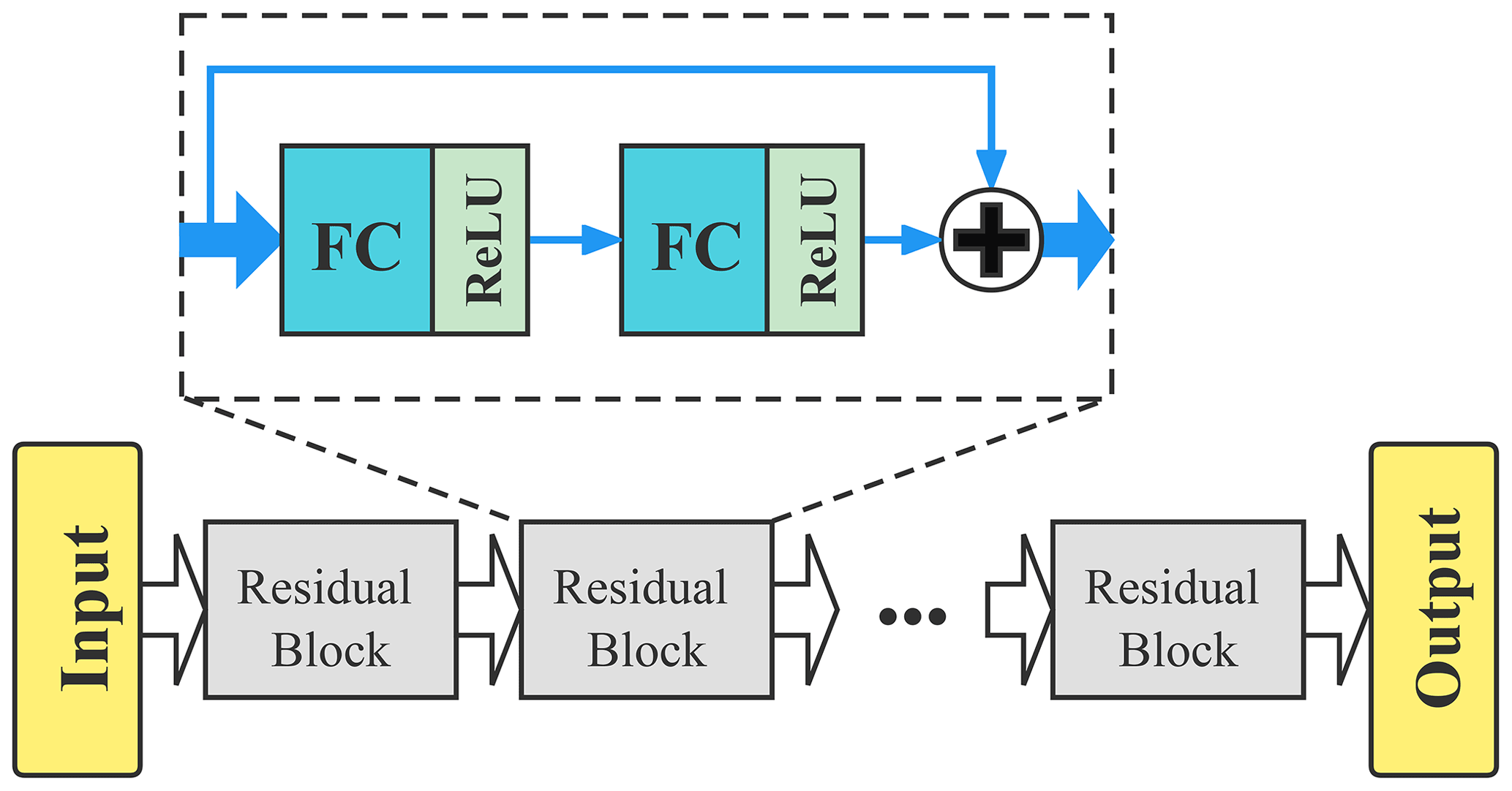
Figure 1Schematic diagram of the structure of the ResDNN. It consists of seven residual blocks, each of which (dashed box) contains two 512-node-wide dense (fully connected) layers with a Rectified Linear Unit (ReLU) (Glorot et al., 2011) as the activation and a layer jump. The inputs and outputs are discussed in Sect. 2.2.2.
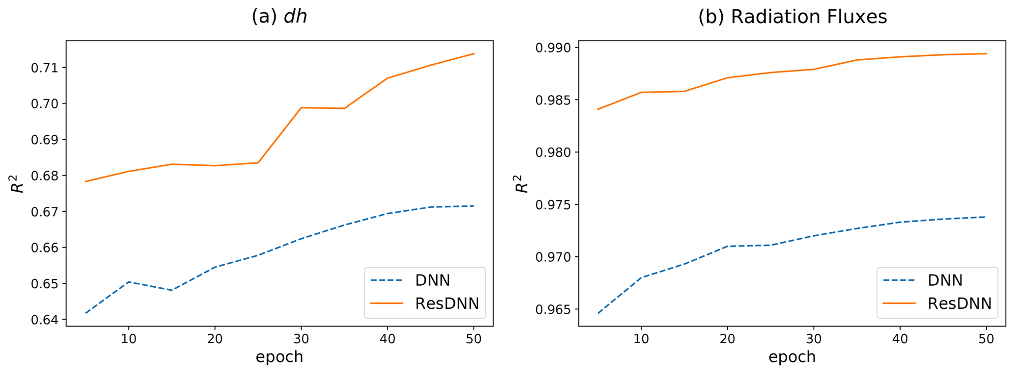
Figure 2Fitting accuracies (R2) of both the proposed ResDNN (solid orange lines) and the DNN (dashed blue lines) for different outputs. (a) The R2 of the moist static energy changing rate (dh) versus the training epochs and (b) the fitting accuracy of the average R2 for the eight radiation fluxes are shown. Note that the R2 values are calculated for both space and time in the validation dataset.
2.2.3 Implementation of NN parameterization
The NN parameterization is implemented into SPCAM to replace both the CRM-based super-parameterization and its radiation effects based on the average of the coarse grid. At the beginning of each time step, NNCAM calls the NN parameterization and predicts the moisture tendency , the dry static energy tendency from the moist physics and radiative heating, and all of the radiation fluxes at the surface and the TOA. Following this, the DNN predictions are returned to NNCAM, and the model states and radiation fluxes are updated. Additionally, the total surface precipitation is derived from the column integration of the predicted moisture tendency. The near-surface conditions of the atmosphere and the downwelling radiation fluxes are transferred to the land surface model. After the land surface model and the prescribed sea surface temperature (SST) are coupled, the host CAM5 performs the planetary boundary layer diffusion and lets its dynamic core complete a time step integration. In the next time step, the dynamic core returns the new model states to the NN parameterization as inputs again. During the entire process, the NN parameterization and GCM constantly update each other's status. Determining a way to couple the NN parameterization with the GCM and to run them efficiently and effectively is the key to the implementation of NNCAM. To solve these problems, we developed the NN–GCM coupler, which integrates the NNs into NNCAM. This process will be introduced in the next section.
2.3 NN–GCM coupler
Deep-learning research mainly uses ML frameworks based on Python interfaces to train neural network models, and they are deployed through C or Python programs. In contrast, GCMs are mainly developed in Fortran, which makes it very challenging to call a neural network model based on a Python or C interface in GCM codes written in Fortran. Solving the problem of code compatibility between the NN and GCM can significantly help develop NN-based parameterizations for climate models.
To implement an NN-based parameterization in the current climate models, which are mostly developed in Fortran, many researchers have attempted to obtain the network parameters (e.g., the weight and bias) from the ML models and implement the NN models (e.g., DNNs) using hard coding in Fortran. At the runtime, NNCAM will call an NN parametrization as a function (Rasp et al., 2018; Brenowitz and Bretherton, 2019). Recently, some researchers have developed a Fortran–neural network interface that can be used to deploy DNNs in GCMs (Ott et al., 2020). This interface can import neural network parameters from outside of the Fortran program, and the Fortran-based implementation ensures that it can be flexibly deployed in GCMs. However, embedding an NN parameterization in NNCAM is still a troublesome task, and there is no existing coupling framework to support many of the latest network structures. This problem prevents researchers from building more powerful NNs and deploying them in NNCAM.
We developed a coupler to bridge the NN parameterization with the host CAM5. Through this coupler, the neural network can communicate with the dynamic core and other physical schemes in NNCAM in each time step. When NNCAM is running (step 1 in Fig. 3), the coupler receives the state and forcing output from the dynamic core in the Fortran-based CAM5. For each input variable, we used the native Message Passing Interface (MPI) interface in CAM5 to gather the data for all of the processes into the master process into a tensor. Following this, the coupler transmits the gathered tensor through the data buffer to the NN parameterization running on the same node as the master process (step 2 in Fig. 3). The NN parameterization obtains the input, infers the outputs, and transmits them back to the coupler. As shown in step 3 in Fig. 3, the coupler writes these tendencies and radiation fluxes back to the master process and then broadcasts the data to the CAM5 processes running on the computing nodes through the MPI transmission interface. Therefore, other parameterizations obtain the predictions from the NN parameterization to complete the follow-up procedures (step 4 in Fig. 3).
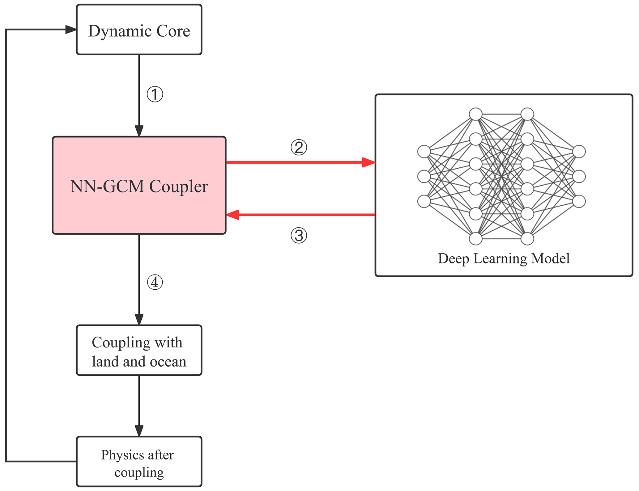
Figure 3A flowchart of NNCAM, including the NN–GCM coupler. NNCAM runs in the direction of the arrow, and each box represents a module. Among them, the NN–GCM coupler is indicated by the pink box. The NN parameterization is shown in the box on the right. In step (1), the dynamic core transmits data to the NN–GCM coupler. In steps (2) and (3), the data communication between the NN–GCM coupler and the NN parameterization takes place. In step (4), the host GCM accepts the results from the NN parameterization.
In practice, the NN–GCM coupler introduces a data buffer that supports a system-level interface, which is accessible by both the Fortran-based GCM and the Python-based NN without supplementary foreign codes. This can avoid code compatibility issues when building ML coupled numerical models. It supports all mainstream ML frameworks, including native PyTorch and TensorFlow. Using the coupler, one can efficiently and flexibly deploy the deep-learning model in NNCAM and can even take advantage of the latest developed neural networks.
All neural network models deployed using the NN–GCM coupler can support a GPU-accelerated inference to achieve excellent computing performance. In this study, we ran SPCAM and NNCAM on 192 CPU cores. NNCAM also used two GPUs for acceleration. During the NNCAM runtime, each time step of NNCAM requires the NN parameterization to complete an inference and conduct data communication with NNCAM. This is a typical high-frequency communication scenario. We evaluated the amount of data (about 20 MB for CAM5 with a horizontal resolution of 1.9∘ × 2.5∘) that needs to be transmitted for each communication and decided to establish a data buffer on a high-speed solid-state drive to ensure a balance between performance and compatibility. It takes about s to access the data buffer in each time step, which is enough to support the efficient simulation of NNCAM. The simulation years per day (SYPD) of NNCAM based on the NN–GCM coupler represents an impressive performance improvement. When using 192 Intel CPU cores, the SYPD of SPCAM is 0.3, the SYPD of CAM5 is 20, and the SYPD of NNCAM is 10. It should be noted that NNCAM based on the NN–GCM coupler uses an additional GPU to accelerate the NN parameterization. When the NN–GCM coupler is not used, the NN parameterization is implemented using Fortran and is accelerated by the Fortran-based Math Kernel Library and the SYPD is 1.5.
3.1 Trial and error
To develop a stable NN parameterization, we propose the use of a set of three ResDNNs, in which each neural network is responsible for predicting a class of variables (see Sect. 2.2.2). Ott et al. (2020) demonstrated that there is a negative correlation between the offline MSE and online stability when using tendencies as outputs in aqua-planet simulations. Since we also used tendencies as outputs in the real-world simulations, we conclude that an NN-based parameterization that can support long-term integration should have a high accuracy regarding training and validation. As was described in Sect. 2.2.2, we tried DNNs first and then extended the DNNs to ResDNNs to achieve a high offline accuracy (Fig. 2). Even though more accurate ResDNNs have a higher probability of becoming stable parameterizations (Fig. 4), we still do not have a way to determine the stability a priori. Therefore, we still used the trial-and-error method to filter out unstable ones and then selected the best ResDNN set that could reduplicate the total energy time evolution of SPCAM with the least deviation, i.e., the NN parameterization.
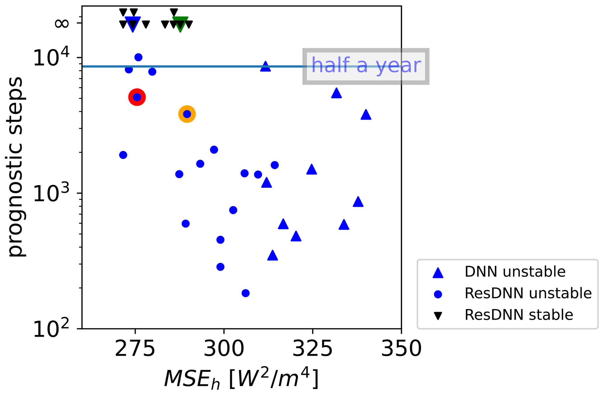
Figure 4The mean square error of the offline moist static energy versus the prognostic steps. The inverted black triangles (the three inverted black triangles are above the infinity line to avoid overlapping) denote stable NN coupled prognostic simulations that last for more than 10 years. The blue dots denote unstable simulations, and the blue triangles denote unstable DNNs. The dots with colored outlines are shown in Fig. 5 for the time evolution of the globally averaged energy.
3.2 Sensitivity tests
We conducted prognostic runs of all three neural networks in each NN set using the NN–GCM coupler. To demonstrate the reality behind the relationships between the offline accuracy and online stability under a real-world configuration, we conducted sensitivity tests using 10 DNN sets and 27 ResDNN sets and conducted the training and evaluation using the settings described in Sect. 2.2.2. In the sensitivity tests, we conducted prognostic runs (see details in Sect. 3.2) using all three neural networks in each NN set using the NN–GCM coupler.
First, we selected the best ResDNN for the radiation fluxes at the surface, and the TOA that was shared in every NN set since their offline validation was exceptionally accurate with R2>0.98 over 50 training epochs (Fig. 2b). In contrast to the accurately trained radiation fluxes, the tendencies of the dry static energy and moisture are less accurate and can affect the prognostic performance. To evaluate those two tendencies using one metric, we introduced the MSE of the rate of change of the moist static energy (:
where g is the acceleration due to gravity, Lv is the latent heat of water vapor, and Δp is the layer thickness. Multiple ResDNN pairs and DNN pairs for dqv and ds were trained from 5 to 50 epochs, resulting in different offline validation accuracies. We used the maximum number of steps until the model crashed to measure the prognostic performance.
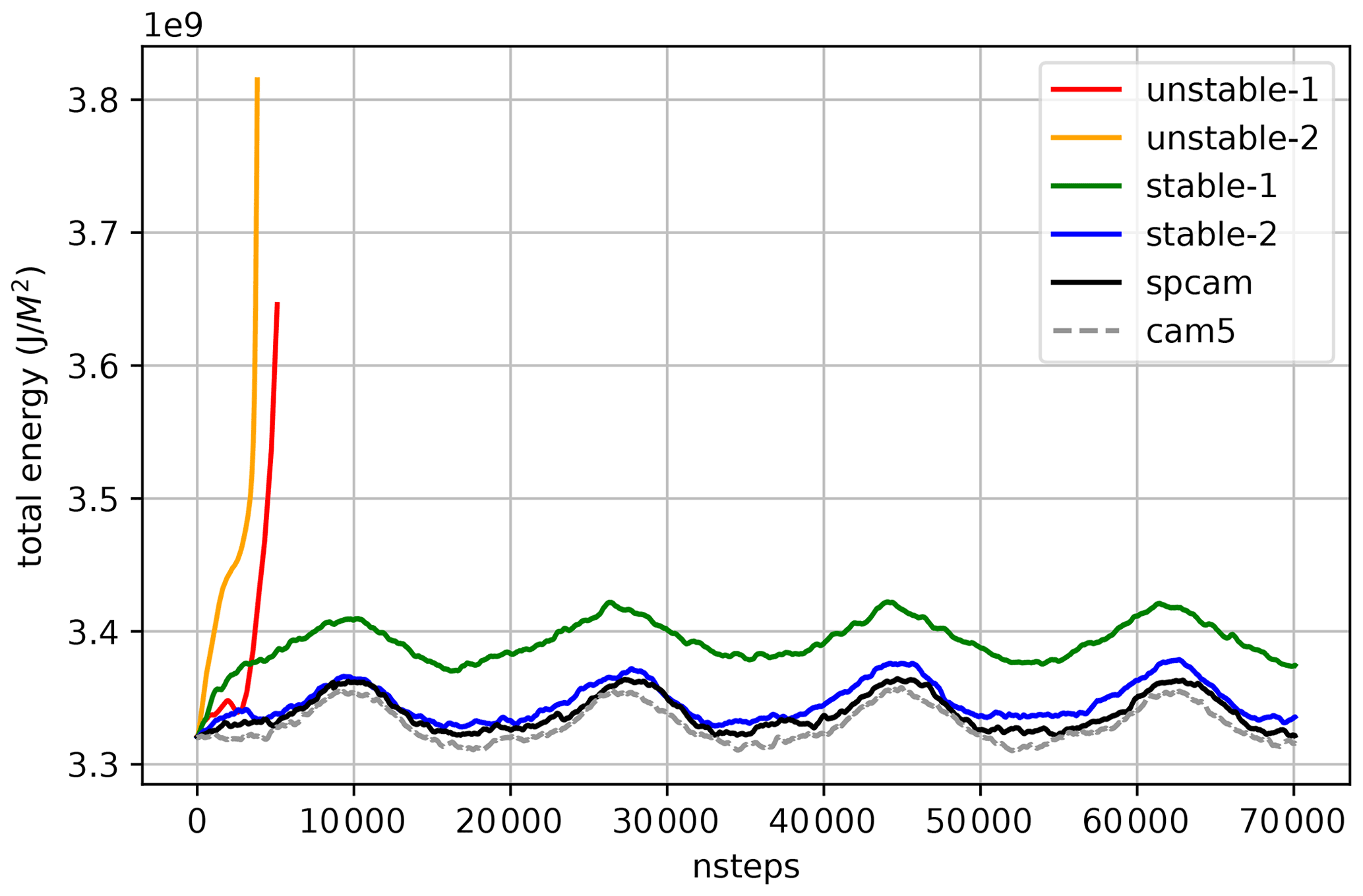
Figure 5Time evolution of the globally averaged column of the integral total energy of NNCAM with different ResDNN parameterizations (marked with the same colors as in Fig. 4), SPCAM target (black line), and CAM5 control run (dashed grey line). The blue line indicates the stable and accurate ResDNN, the green line indicates the stable but deviating ResDNN, and the orange and red lines indicate unstable ResDNNs.
Figure 4 shows the offline validation MSEh versus the maximum prognostic steps. The DNN parameterizations (blue triangles) are systematically less accurate than the ResDNN parameterizations (blue dots and inverted black triangles), which is consistent with Fig. 2a. They could not sustain half a year of simulation in the prognostic tests with the best DNN parameterization. For the ResDNNs, the less well-trained ones with high MSEs also crashed after short simulation periods. However, when the offline MSE decreased to a certain level (e.g., 290 W2 m−4), 10 of the ResDNN parameterizations were stable in long-term simulations of over 10 years (black inverted triangles). We speculate that the more accurate ResDNN sets have a higher probability of becoming stable NN parameterizations since all of the stable NN parameterizations are ResDNNs.
A few unstable ResDNN sets are equally or more accurate than the stable ones. Previous studies have shown that high-capacity (more hidden layers and more weights and biases) models are harder to train and are more likely to produce overfitting (Goodfellow et al., 2016). Some overly trained ResDNNs with lowest validation loss are speculated to produce overfitting, and they are therefore less likely to generalize to unknown backgrounds caused by accumulated errors in the ML–GCM system, causing the model to crash.
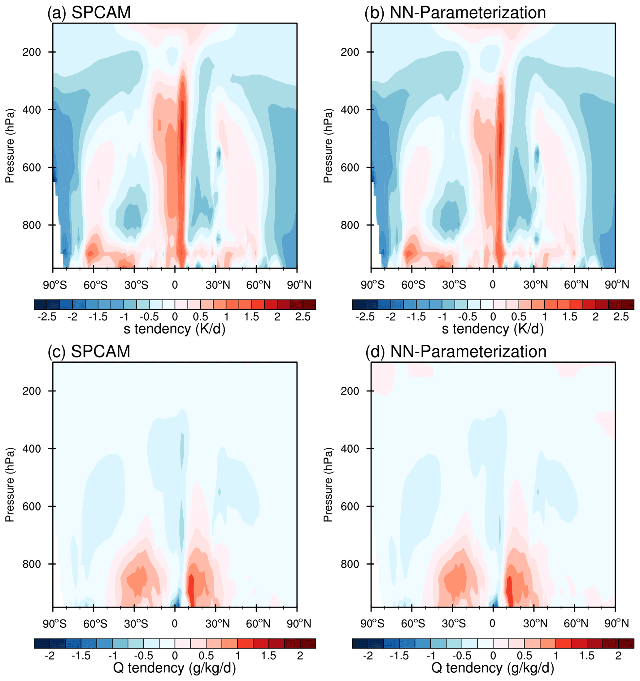
Figure 6Latitude–pressure cross sections of the annual and zonal mean heating (top) and moistening (bottom) due to moist physics during the year 2000 for (a, c) SPCAM simulations and (b, d) the offline test using the NN parameterizations.
In the time evolution of the globally averaged total energy (Fig. 5), the system energy grows exponentially and then blows up for unstable ResDNN parameterizations (the red and orange lines). In contrast, the stable ones can keep the total energy at a certain level and reproduce the annual cycle of fluctuations in SPCAM. Among the stable ResDNN sets, some can almost perfectly reproduce the total energy evolution of SPCAM (the blue line). However, some inaccurately simulate the climate state with a significant deviation (green line). Apart from global averages, the prognostic results of the 10 stable ResDNN sets vary from each other in terms of the global distribution. Figure S1 shows the precipitation spread across all of the stable NN sets for the prognostic simulation from 1999 to 2003. The obvious standard deviation centers coincide with the heavy tropical precipitation areas.
3.3 Gravity wave diagnosis
It is still unclear why unstable NN parameterizations blow up models. The fast-growing energy of the unstable runs indicates a possible underlying unrealistic energy amplifying mechanism in the coupled NN–GCM system. Brenowitz et al. (2020) offered several interpretations. When an unstable NN parameterization is coupled with dynamics, it tends to amplify any unrealistic perturbations caused by emulation errors and pass it to the entire system through gravity waves. In contrast, the stable NN parameterizations tend to dump all of the perturbations quickly. This was found to be true in our study for the realistic configuration. Such unstable gravity waves were observed in the prognostic simulation of an unstable ResDNN (red line in Fig. 5). The animation in Movie S1 records the first unrealistic wave, and Movie S2 documents the more intense waves with a perfectly round shape after this point in time. Additionally, we found that our instable waves mostly occurred in the tropics, which is different from the mid-latitude instability that occurs when using ML parameterizations in aqua-planet simulations (Brenowitz et al., 2020).
Brenowitz et al. (2020) also introduced an analysis tool that calculates the wave energy spectra of a hierarchy model that couples the linear response functions (LRF) of an NN-based parameterization to a simplified two-dimensional linear dynamic system, in which perturbations can propagate in 2-D gravity waves. We applied the tool in this study and detected similar results in the unstable mode for the unstable ResDNN with a positive energy growth rate across all wave numbers at phase speeds of 5–20 m s−1 (Fig. S2b). In contrast, the stable ResDNN exhibited a stable mode for the growth rate of nearly all wave numbers and phases below zero (Fig. S2a).
Before evaluating the prognostic results, the offline performance with geographic information needs to be demonstrated for the following purposes: (1) to show how well our NN parameterization emulates the SP for a realistic configuration compared with the baseline CAM5 physics and previous studies and (2) to reveal the strengths and weaknesses of the NN emulations with the correct input and to provide clues to the analysis of the prognostic results in the following section. We performed offline testing using a realistically configured SPCAM from 1 January 1999 to 31 December 2000, in which the NN parameterization was diagnostically run parallel to the SP in addition to the CAM5 physics. The results for the entire second year of the simulation period were chosen for evaluation, which was completely independent from the training dataset. Following the conventions of Han et al. (2020) and Mooers et al. (2021), we used the mean fields and the coefficient of determination (R2) as the evaluation metrics. It should be noted that the NN parameterization was tuned to emulate the SP, and the CAM's parameterization was tuned to obtain close results to the observations. The latter is merely introduced as a baseline.
The mean diabatic heating and drying rates produced by convection, large-scale condensation, and cloud radiation effects in SPCAM and the NN parameterization are in close agreement. Figure 6 shows the latitude–height cross sections of the annual mean heating and moistening rates in SPCAM and the corresponding NN parameterization. At 5∘ N, SPCAM exhibits the maximum latent heating in the deep troposphere, corresponding to the deep convection in the ITCZ. In the subtropics, heating and moistening occur in the lower troposphere, corresponding to the stratocumulus and shallow convection in the subtropics. In the mid-latitudes, there is a secondary heating maximum below 400 hPa due to the mid-latitude storm tracks. All of these features are well reproduced by the NN parameterization. It should be noted that the peak in the drying rate in the ITCZ in the mid-troposphere is slightly weaker in the NN parameterization than in SPCAM (Fig. 6c and d).
In addition to the mean fields, the high prediction skill of the NN parameterization is also demonstrated by the spatial distribution of the R2 values. To illustrate the R2 values of the 3-D variables, such as the diabatic heating and moistening, the zonal averages were calculated in advance before the R2 calculation for each location in the pressure–latitude cross section following Mooers et al. (2021). For the diabatic heating, the R2 value is >0.7 throughout the middle and lower troposphere, and the high-skill regions with R2 values of greater than 0.9 are concentrated in the low levels but extend into the mid-troposphere in the storm tracks (Fig. 7a). For the moistening rate, the high skill zones are concentrated in the middle and upper troposphere (Fig. 7b), with low skill areas below. The regions with lower accuracies are generally located in the middle and lower troposphere in the tropics and subtropics, which correspond to the deep convection in the ITCZ and the shallow convection in the subtropics. Nonetheless, the tendencies of the diagnostic CAM5 parameterization are not similar to those simulated by the SP, except for a few locations in the middle and upper troposphere in the tropics and polar regions (Fig. 7c and d).
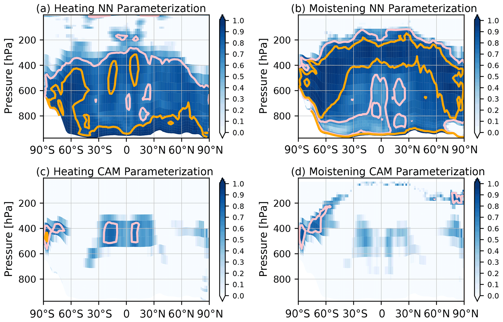
Figure 7Latitude–pressure cross sections of the coefficient of determination (R2) for the zonally averaged heating (a, c) and moistening (b, d) predicted using (a, b) the NN parameterization in the offline 1-year SPCAM run, and (c, d) the offline CAM5 parameterizations. Both were evaluated at a 30 min time step interval. Note that the areas where R2 is greater than 0.7 are contoured in pink, whereas the areas where R2 is greater than 0.9 are contoured in orange.
The global distribution of the R2 values of the precipitation predictions is shown in Fig. 8. Our NN parameterization produced excellent predictions in most of the in mid- and high-latitude regions, especially in the storm tracks. However, the prediction skill is relatively low in many of the ocean areas between 30∘ S and 30∘ N and in some mid-latitude areas over continents (Fig. 8a). In particular, the results are not ideal along the equatorial regions, in the subtropical Eastern Pacific, and in the subtropical Eastern Atlantic. These areas correspond to the low skill zones of the moistening rate in the middle and lower troposphere from the Equator to the subtropics (Fig. 7b). As a baseline, the total precipitation simulated using the CAM5 parameterizations is much less analogous to the SP than the NN parameterization and has a systematically lower accuracy globally. The CAM5 precipitation can achieve a relatively high accuracy along the mid-latitude storm tracks, but it fails in most regions in the tropics (Fig. 8b).
Generally, the NN parameterization performed far better than the CAM5 parameterization in the 1-year period in the offline testing, and it had an accuracy similar to that of the DNN used by Mooers et al. (2021). The use of real geographic data can significantly decrease the emulation skill of a deep-learning model (Mooers et al., 2021). This is because the convection backgrounds of real geographic data are much more complex with meridional and zonal asymmetric and seasonally varying circulations. In addition, the orography and various types of underlying land surfaces also add complexity. In this case, the ResDNN is a valuable NN architecture that performs well as an automated hyperparameter tuning algorithm that does not need to search for hundreds of NN candidates. Our NN parameterization still produced low-accuracy predictions along the Equator over the oceans where the convection is complex and vigorous and in subtropical ocean areas where the convection is weak and concentrated at low levels. This indicates that the NN parameterization is still inadequate in rems of its emulation skill when simulating various types of deep and shallow convection in the tropics.
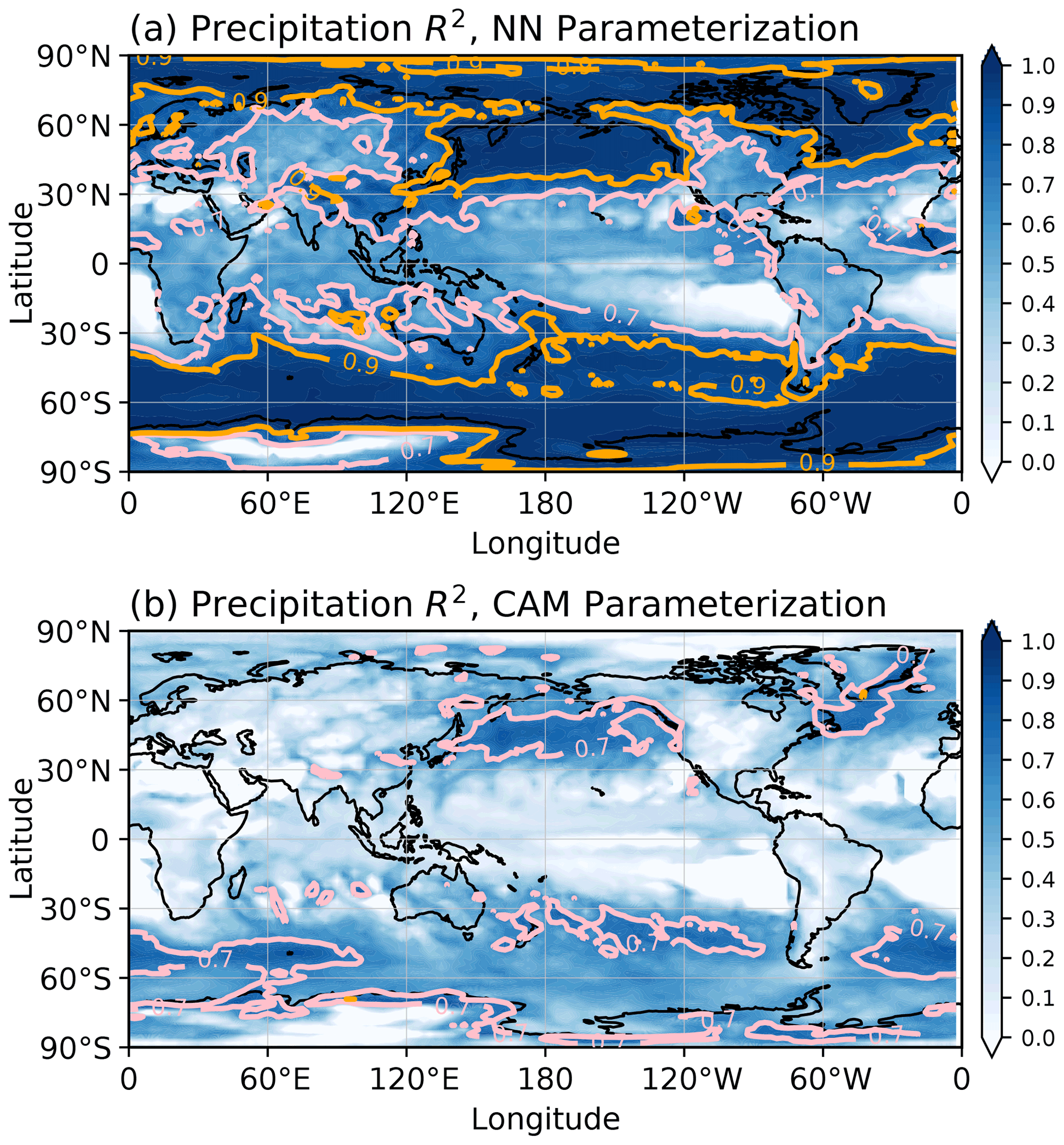
Figure 8Latitude–pressure cross sections of the coefficient of determination (R2) for the time sequence at each location for (a) the derived precipitation predicted using the NN parameterization and (b) the total precipitation from the CAM5 parameterization compared to the offline 1-year SPCAM run. The predictions and SPCAM targets are for a 30 min time step interval. Note that the areas where R2 is greater than 0.7 are contoured in pink, whereas the areas where R2 is greater than 0.9 are contoured in orange.
The NN parameterization produced the best prognostic performance in Sect. 3.1. It was coupled in the realistically configured SPCAM to replace the SP and its cloud-scale radiation effects. This coupled model is referred to as NNCAM hereinafter and is compared with SPCAM and CAM5. The start time of all three models was 1 January 1998. They were all run for 6 years, with the first year used as spin up and the next 5 years (1 January 1999 to 31 December 2003) used for evaluation and comparison. Later, the simulation of NNCAM was extended for another 5 years (to 31 December 2008) to demonstrate its stability. Due to the excessive computing resources required, the SPCAM simulation was not extended. In the analysis of the prognostic results, the following variables were selected to demonstrate the multi-year climatology and variability:
-
the mean temperature and humidity fields,
-
the mean precipitation field,
-
the precipitation frequency distribution,
-
the Madden–Julian Oscillation.
As was mentioned in the Sect. 1, SPCAM, which uses the 2-D SAM as the SP, does not simulate mean climate states better than its host coarse-grid model CAM5, but it excels in climate variability. What is remarkable about NNCAM is not its performance in simulating the mean climate but its ability to achieve a stable multi-year prognostic simulation under a real-world global land–ocean distribution. The advantages and problems of this study will provide important references for future research on NN-based stable long-term model integrations.
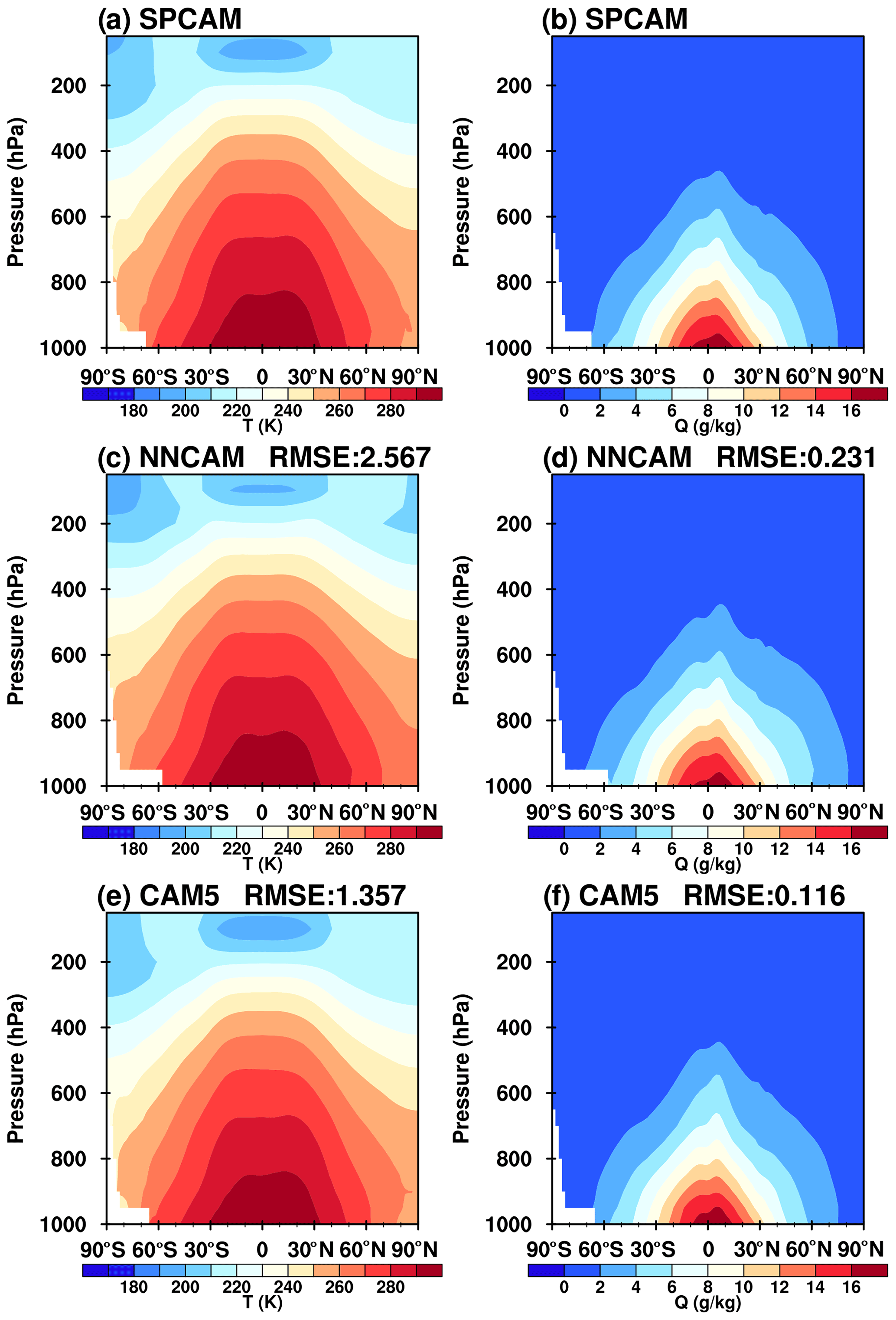
Figure 9Latitude–pressure cross sections of the zonal mean temperature (a, c, e) and specific humidity (b, d, f) averaged from 1999 to 2003 predicted using (a, b) SPCAM, (c, d) NNCAM, and (e, f) CAM5.
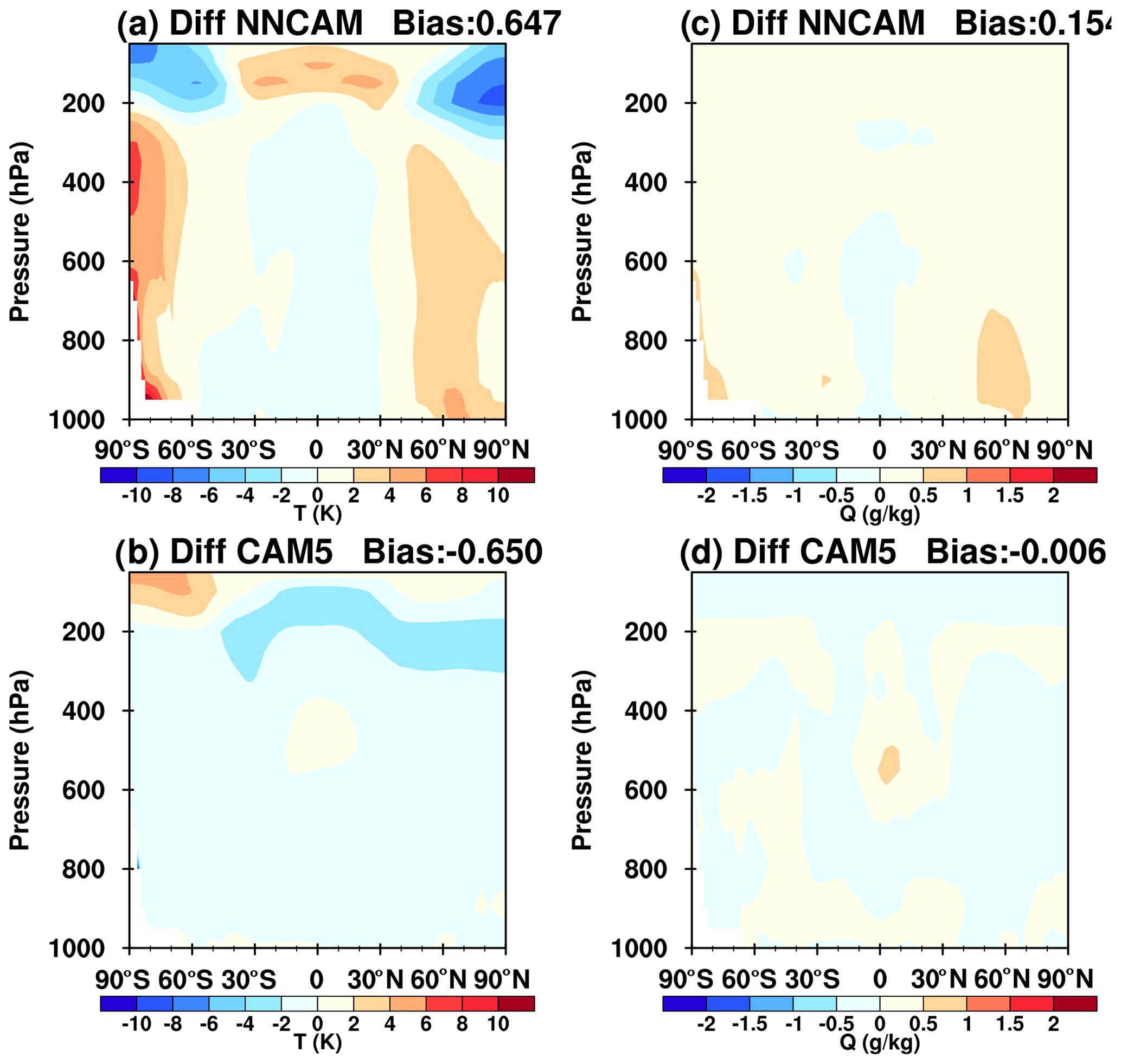
Figure 10Latitude–pressure cross section of the zonal and annual mean differences in the temperature (a, b) and specific humidity (c, d) between (a, c) NNCAM and SPCAM and (b, d) CAM5 and SPCAM. The simulation period for all of the models was from 1999 to 2003.
5.1 Climatology
5.1.1 Vertical profiles of temperature and humidity
In this section, we evaluate the vertical structures of the mean temperature and humidity fields. Figure 9 shows the zonally averaged vertical profiles of the air temperature and specific humidity simulated using NNCAM and CAM5 compared to the SPCAM simulations. Overall, NNCAM simulated reasonable thermal and moisture structures. However, the multi-year mean temperature and moisture fields produced by NNCAM are more biased than those produced by CAM5, which is reflected by the larger root-mean-square errors (RMSEs) (Fig. 9) and larger differences compared to those of CAM5 (Fig. 10). The larger deviations are temperature biases in the tropopause. In this region, the cold-point region is thinner and warmer in NNCAM than in SPCAM and CAM5. In addition, there are cold biases above 200 hPa and warm biases blow over the polar regions in NNCAM. For the humidity field, there are slight dry biases over the Equator and wet biases elsewhere in NNCAM. Even with these biases, the mean climate states are consistent with those in the last 5 years of the simulation for NNCAM (Fig. S3), which indicates that the climate states simulated by NNCAM are constant in the long-term simulation.
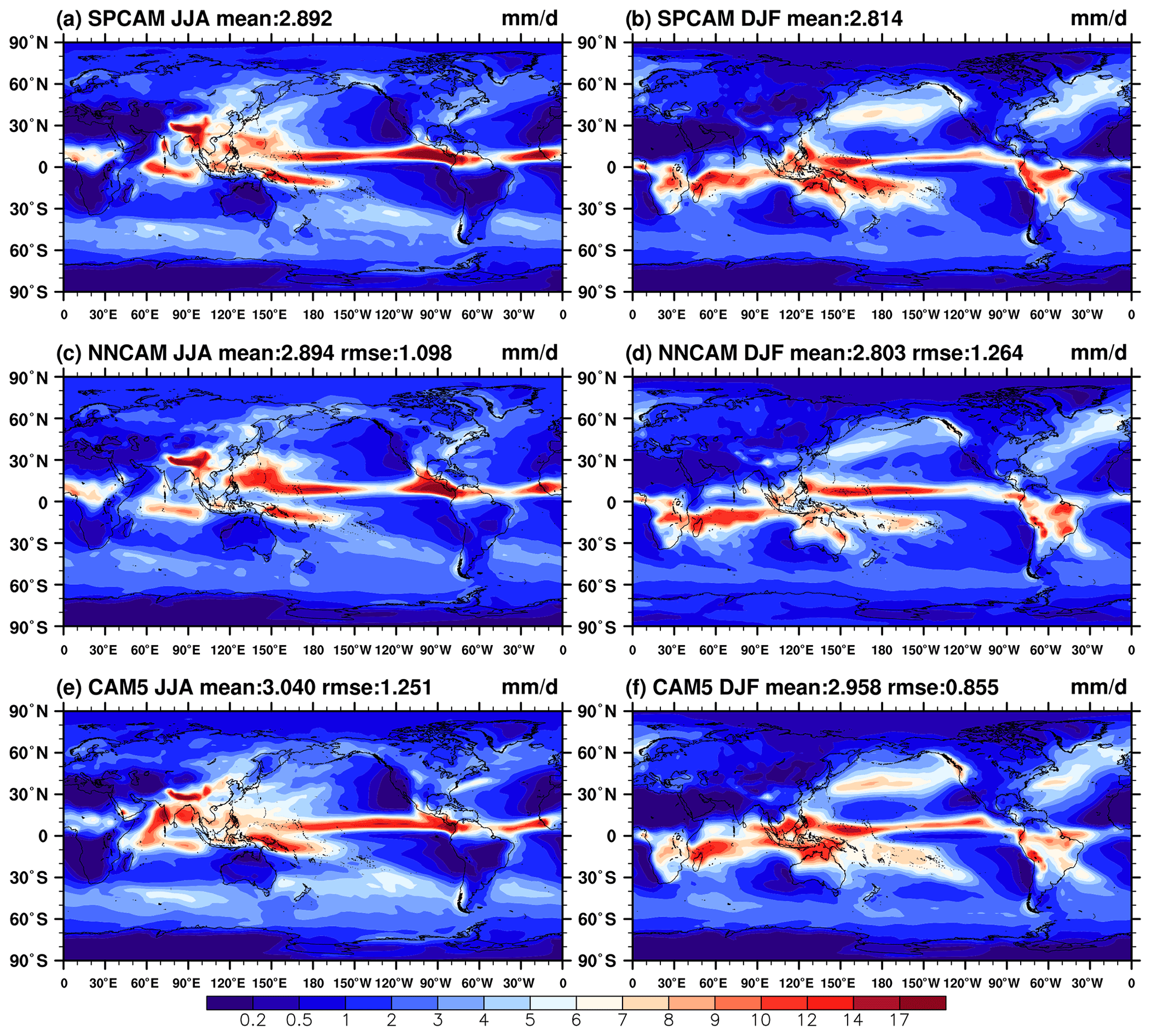
Figure 11The mean precipitation rate (mm d−1) averaged from 1999 to 2003 for June–July–August (a, c, e) and December–January–February (b, d, f) predicted using (a, b) SPCAM, (c, d) NNCAM, and (e, f) CAM5.
5.1.2 Precipitation
Figure 11 shows the spatial distributions of the winter (December–January–February) and summer (June–July–August) mean precipitation simulated using SPCAM, NNCAM, and CAM5. The SPCAM simulation results are regarded as the reference precipitation. In SPCAM (Fig. 11a and b), massive precipitation can be observed in the Asian monsoon region and the mid-latitude storm tracks over the northwest Pacific and Atlantic oceans. In the tropics, the primary peaks in the rainfall occur in the eastern Indian Ocean and Maritime Continent regions. In addition, two zonal precipitation bands are located at 0–10∘ N in the equatorial Pacific and Atlantic oceans, constituting the northern ITCZ. The southern South Pacific Convergence Zone (SPCZ) is mainly located at around 5–10∘ S near the western Pacific warm pool region and tilts southeastward as it extends eastward into the central Pacific. The main spatial patterns of the SPCAM precipitation are properly reproduced by both NNCAM and CAM5. For NNCAM, the strong rainfall centers are well simulated over the tropical land regions of the Maritime Continent, the Asian monsoon region, South America, and Africa (Fig. 11c and d). In addition, the heavy summertime precipitation over the Northwestern Pacific simulated by SPCAM is well represented by NNCAM (Fig. 11a and c). For CAM5, there is too little precipitation over this area (Fig. 11e). Moreover, NNCAM maintained the spatial pattern and global average of the precipitation in the next 5 years of the simulation, demonstrating its long-term stability (Fig. S4).
Generally, the NNCAM results are more similar to SPCAM than the CAM5 results in terms of the spatial distribution of the summertime multi-year precipitation, with smaller RMSEs and globally averaged biases. However, on a difference plot (Fig. S5), NNCAM moderately underestimates the precipitation along the Equator, in the Indian monsoon region, and over the Maritime Continent in the summer (Fig. S5a). In the boreal winter, NNCAM simulates a weak SPCZ that is excessively separated from the ITCZ, with both precipitation centers shifted away from each other. As a result, underestimation occurs in the equatorial regions of the Maritime Continent and in the SPCZ, while overestimation occurs to the north of the Equator in the western Pacific (Fig. S5b); thus, NNCAM resembles SPCAM less than CAM5 in this season. This underestimation of the precipitation along the Equator can also be observed in the zonal mean multi-year precipitation plots (Fig. 12). There is a more significant minimum zone in the equatorial precipitation near the Equator compared with in SPCAM and CAM5 for the annual average (Fig. 12a) and the boreal winter average (Fig. 12c).
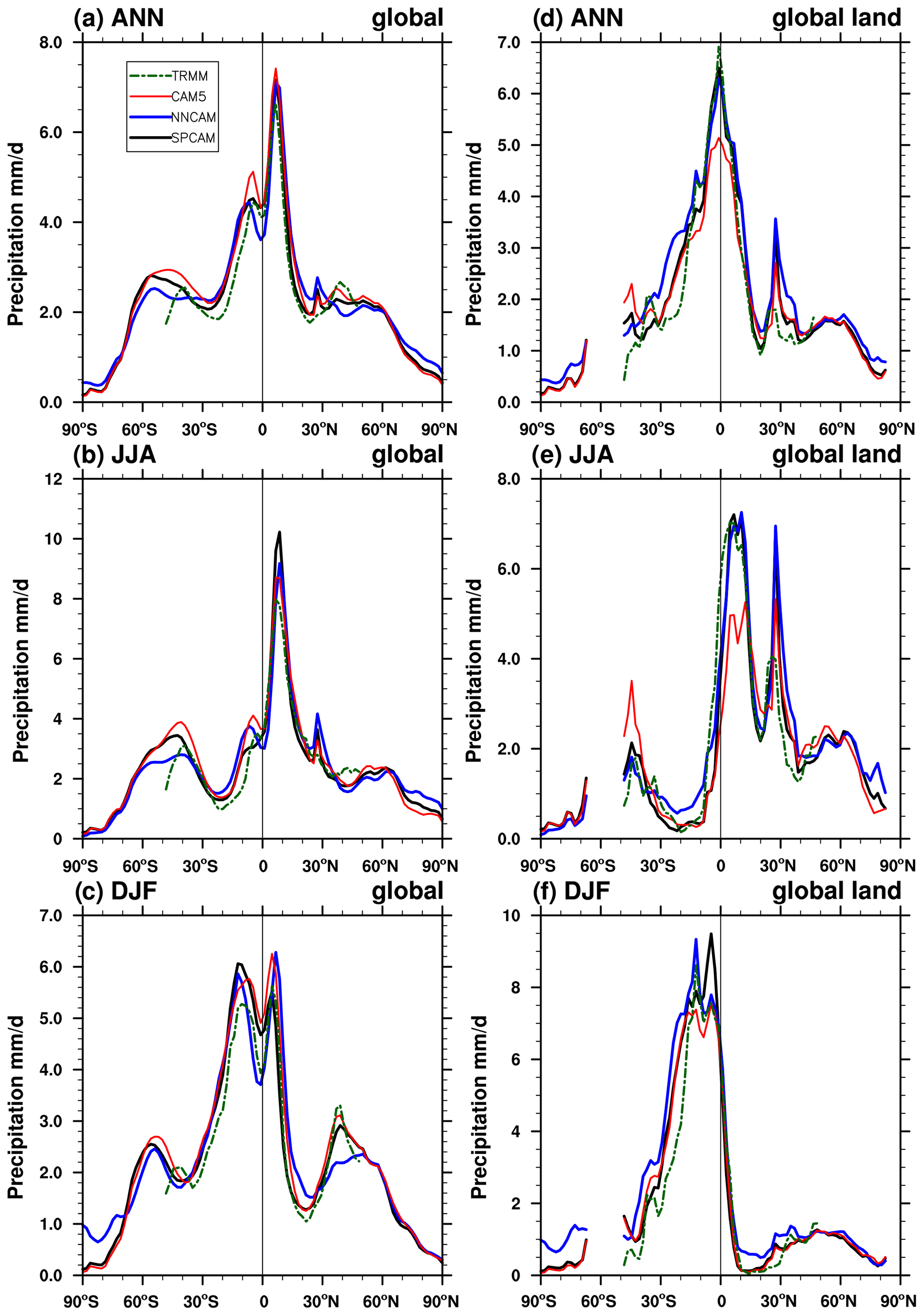
Figure 12The zonal mean precipitation rate (mm d−1) averaged from 1999 to 2003 for (a, d) the annual mean, (b, e) June–July–August, and (c, f) December–January–February. The black, blue, and red solid lines denote SPCAM, NNCAM, and CAM5, respectively. The dashed dark green line denotes the averaged results of the TRMM 3B42 daily rainfall product.
In contrast to the oceanic rainfall, NNCAM predicts the precipitation over the land surfaces with good skill in the tropics (land fraction equal to 1), which resembles the tropical land rainfall intensity of SPCAM and Tropical Rainfall Measuring Mission (TRMM) (Huffmann et al., 2007) observations of the annual and boreal summer averages (Fig. 12d and e). According to Kooperman et al. (2016), SPCAM predicts the Asian and African monsoon activity better, which leads to the more accurate land rainfall in such areas. This is related to the stronger convective variability in the SP than the conventional parameterizations. As an emulator of SPCAM, NNCAM inherits this strength.
5.2 Variability
5.2.1 Frequency distribution of precipitation
Moreover, NNCAM exhibited a better performance in simulating the precipitation extremes. Figure 13 shows the probability density function of the simulated daily precipitation in the tropics (30∘ S–30∘ N) with a precipitation intensity interval of 1 mm d−1. For CAM5, the heavy precipitation events exceeding 20 mm d−1 are greatly underestimated. In addition, for CAM5, the light to moderate precipitation events (2–20 mm d−1) are overestimated, with an unreal probability peak around 10 mm d−1, which is a typical simulation bias found in simulations with parameterized convection and no explicitly resolved convection (Holloway et al., 2012). Compared with CAM5, the spectral distribution of the precipitation for NNCAM is much closer to that of SPCAM. The heavy rainfall events are substantially enhanced, and the overestimated moderate precipitation (2–20 mm d−1) is reduced, with no spurious peak at around 10 mm d−1.
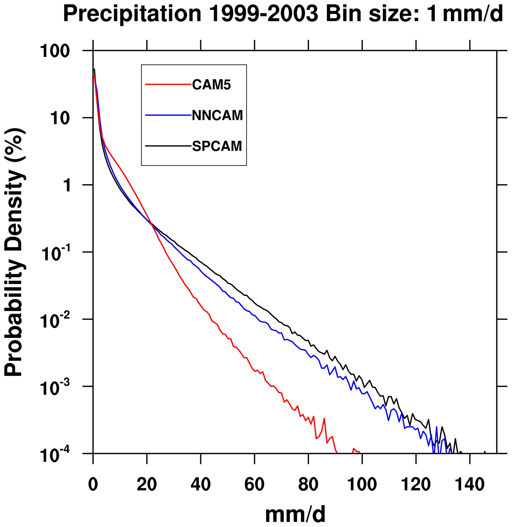
Figure 13Probability densities of the daily mean precipitation in the tropics (30∘ S–30∘ N) obtained from the three model simulations. The black, blue, and red solid lines denote SPCAM, NNCAM, and CAM5, respectively.
5.2.2 The MJO
The MJO is a crucial tropical intraseasonal variability that occurs on a timescale of 20–100 d (Wheeler and Kiladis, 1999). Figure 14 presents the wavenumber and frequency spectra for the daily equatorial precipitation anomalies for SPCAM, NNCAM, and CAM5 in four consecutive boreal winters from 1999 to 2003. SPCAM shows widespread power signals over zones 1–4 and periods of 20–100 d, as well as a peak around zone numbers 1–3 and periods of 70–100 d for the eastward propagation (Fig. 14a). Similarly, for NNCAM, there is a spectral peak at wavenumbers of 1–2 and periods of 50–80 d for the eastward propagation (Fig. 14b), exhibiting intense intraseasonal signals. For CAM5 (Fig. 14c), the spectral power is concentrated around 30 d and exhibits more extended periods (greater than 80 d) at a wavenumber of 1 for the eastward propagation. In addition, CAM5 also shows signals of westward propagation with a 30 d period. Compared with CAM5, NNCAM exhibits stronger intraseasonal power and resembles SPCAM better. To quantify this similarity, we calculated the coefficients of determination R2 for the precipitation spectra of NNCAM and CAM5 using the spectrum of SPCAM as the target value. The R2 value of the precipitation spectrum NNCAM (0.51) is much higher than that for CAM5 (0.40).
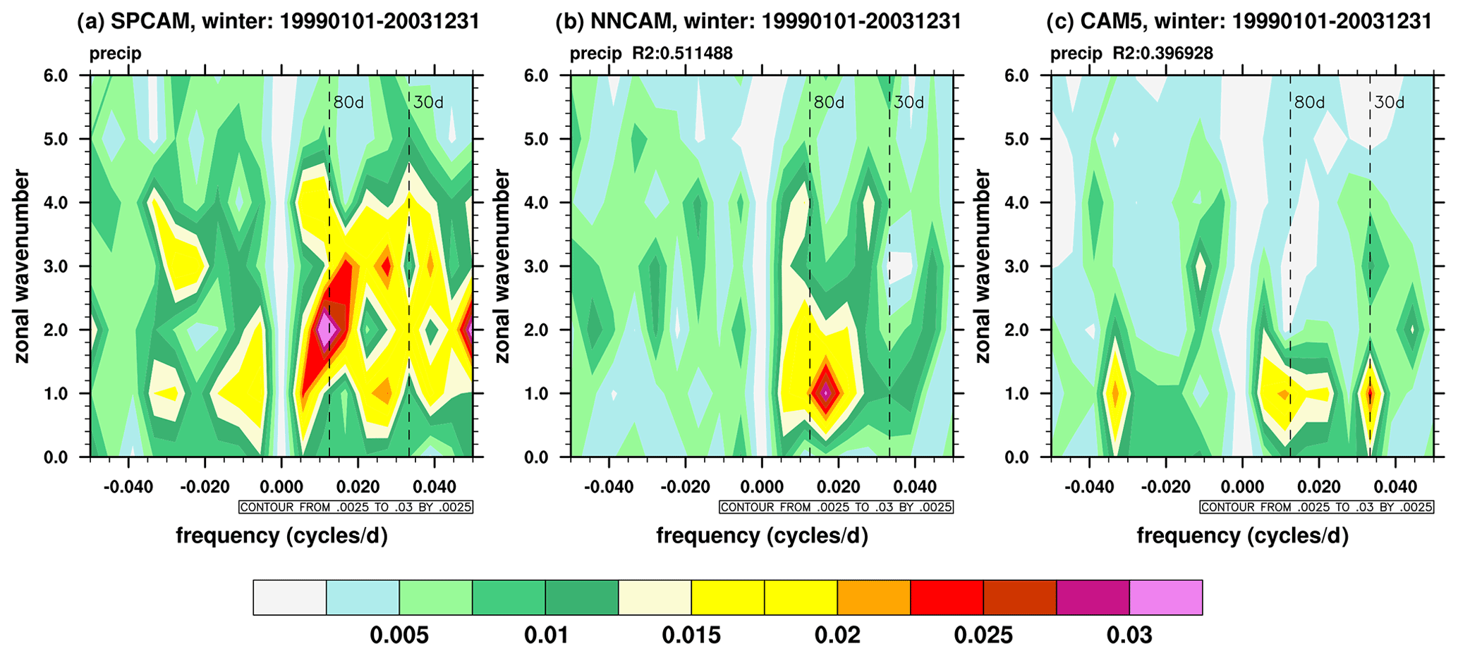
Figure 14The wavenumber–frequency spectra for the daily precipitation anomalies at 10∘ S–10∘ N for (a) SPCAM, (b) NNCAM, and (c) CAM5 simulations in boreal winter.
The MJO is characterized by the eastward propagation of deep-convective structures along the Equator. Generally, it forms over the Indian Ocean, strengthens over the Pacific Ocean, and weakens over the eastern Pacific Ocean due to interactions with cooler SSTs (Madden and Julian, 1972). Figure 15 presents the longitude-time lag evolution for the 10∘ S–10∘ N meridional averaged daily anomalies of the intraseasonal (filtered using a 20–100 d bandpass) precipitation and 200 hPa zonal wind (U200) in the boreal winter. The results show that both SPCAM and NNCAM reasonably reproduce the eastward propagation of the convection from the Indian Ocean across the Maritime Continent and into the Pacific (Fig. 15a and b). This is confirmed by both the precipitation field and U200 field. Therefore, we conclude that NNCAM captures the key MJO propagation simulated by SPCAM. In contrast, the time lag plot for CAM5 depicts an inaccurate westward propagation. Similar to the precipitation spectrum, the R2 value of the time lag coefficient is shown to quantify the similarities between the simulations. The time lag coefficient of the U200 field for NNCAM is much closer to that for SPCAM than CAM5, with a much higher R2 value, indicating that the NN parameterization successfully emulates the convection variability of the SP, which is reflected in the dynamic fields.
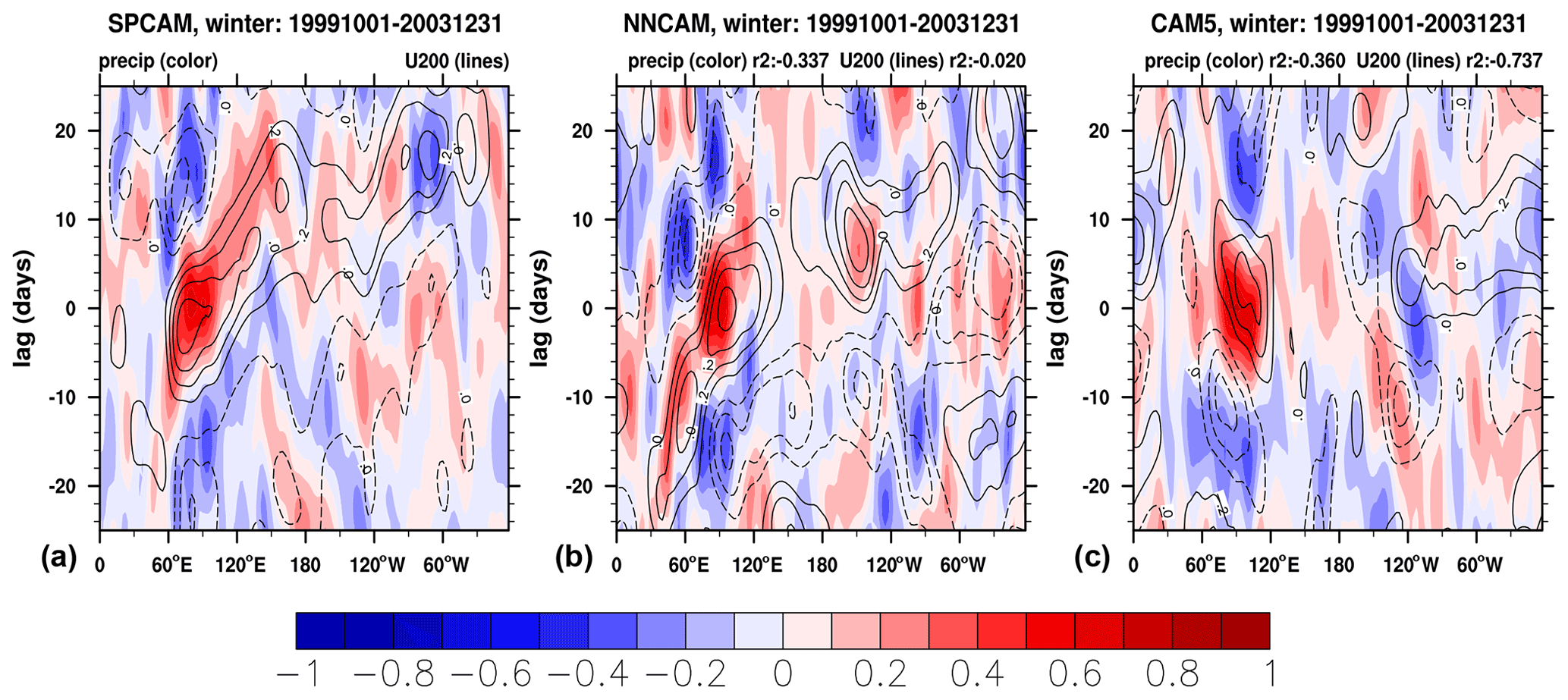
Figure 15Longitude–time evolution of the lagged correlation coefficient for the 20–100 d bandpass-filtered precipitation anomalies (averaged over 10∘ S-−10∘ N) against the regionally averaged precipitation (shading) and zonal wind at 200 hPa (contours) over the equatorial eastern Indian Ocean (10∘ S−-10∘ N, 80−-100∘ E) for (a) SPCAM, (b) NNCAM, and (c) CAM5.
In this study, the potential of deep neural network-based parameterizations in SPCAM to reproduce long-term climatology and climate variability was investigated. We developed an NN parameterization via a ResDNN set to emulate the SP with a 2-D CRM and its cloud-scale radiation for a realistically configured SPCAM with a true land–ocean distribution and orography. The input variables of the NN parameterization include the specific humidity, temperature, large-scale water vapor and temperature forcings, surface pressure, and solar insolation. The output variables of the NN parameterization include the subgrid tendencies of the moisture and dry static energy and the radiation fluxes. We propose a set of 14-layer deep residual neural networks, in which each NN is in charge of one group of output variables. With such a design, we gained a best emulation accuracy for each predictor. Through systematic trial-and-error searching, we were able to select sets of ResDNNs that support stable prognostic climate simulations, and we then chose the best set with the lowest climate errors as the formal NN parameterization. Moreover, the mechanism of the unreal perturbation amplification was identified in the GCM simulations with unstable NN parameterizations using the spectrum diagnostic tool invented by Brenowitz et al. (2020).
The offline tests demonstrated the good skills of the NN parameterization in emulating the SP outputs and the cloud scale radiation effects of SPCAM. The overall diabatic heating and drying rates in the NN parameterization and SPCAM are in close agreement. When implemented in the host SPCAM to replace its time-consuming SP and its radiation effects, the NN parameterization successfully produced an extensive stable long-term prognostic simulation and predicted reasonable mean vertical temperature and humidity structures and precipitation distributions. Compared with the SPCAM target simulation, NNCAM still produces some biases in the mean fields, such as a warmer troposphere over the polar regions and in the tropopause and underestimation of strong precipitation in the equatorial regions. In addition, the better climate variability of SPCAM compared to CAM5 was learned well by our NN parameterization and was reproduced by NNCAM, with better frequency for extreme rainfall and a similar MJO spectrum, propagation direction, and speed. Despite the current biases in the climate states, NNCAM can still be regarded as a first attempt to couple a NN-based parameterization and a realistically configured 3-D GCM.
Many previous studies have investigated ML parameterizations implemented in aqua-planet configured 3-D GCMs. Some faced instability problems in coupled simulations (Brenowitz and Bretherton, 2019), while others succeeded in producing stable long-term prognostic simulations with deep fully connected neural networks (Rasp et al., 2018; Yuval et al., 2021), as well as random forest algorithms (Yuval and O'Gorman, 2020). In contrast to aqua-planet simulations, the spatial heterogeneity is prominent over the land in GCMs, which are configured using real geographic boundary conditions. The convection, clouds, and interactions with the radiation in the CRM and the real geographic boundary conditions are without a doubt far more complicated than in idealized models. To meet the new demand for realistic configurations, we designed a ResDNN with sufficient depth to further improve the nonlinear fitting ability of the NN parameterization. With the skip connections, the 7-layer DNN models can be extended to 14 layers, thereby significantly improving the offline accuracy. In the prognostic tests, a dozen ResDNN parameterizations supported a stable long-term run, while all of the DNN parameterizations tested were found to be unstable.
Trial and error is still our only way to find stable NN-based parameterizations. Thus far, we have not developed an a priori method that guarantees stability. However, we did find some clues in the sensitivity tests. We believe sufficient offline accuracy is essential for online stability and can be achieved by confirming all of the inaccurate NN parameterizations as unstable. In addition, some of the highly accurate ones still crash the prognostic simulation. In this case, the total energy was found to increase rapidly. This mechanism is that unstable NNs cannot damp the neural network emulation errors, and they amplify and propagate them to the entire system through gravity waves.
The prognostic biases of the mean fields are speculated to be a result of the combined effect of the emulation errors of all of the NN parameterization prediction fields. Further study is required. Still, it may be related to the spatially non-uniform accuracy of the NN parameterization, such as the relatively low fitting accuracy in the tropical deep-convective regions and the shallow subtropical convection and stratiform cloud regions. Such problems have also been reported in previous studies (Gentine et al., 2018; Mooers et al., 2021). We believe that an NN parameterization with heterogeneous characteristics across different regions, rather than a globally uniform scheme, can further improve the fitting accuracy in these tropical and subtropical regions.
Embedding deep neural networks into Fortran-based atmospheric models is still a handicap. Before this study, researchers mainly used hard coding to build neural networks (Rasp et al., 2018; Brenowitz and Bretherton, 2019). An easier method is to use Fortran-based neural network libraries that can flexibly import network parameters (Ott et al., 2020). These methods have been used to successfully implement NNs in GCMs, but they can only support dense, layer-based NNs. As a result, developers cannot take advantage of the most advanced neural network structures, such as convolution, shortcut, self-attention, and variational autoencoder structures, to build powerful ML-based parameterizations. In this study, using an NN–GCM coupler, the NN parameterization could support the mainstream GPU-enabled ML frameworks. Thanks to the simple and effective implementation of the NN–GCM coupler, our NNCAM achieved an SYPD 30 times that of SPCAM by using a ResDNN set and NN parameterization, even though these DNNs are much deeper than the previous state-of-the-art fully connected NNs in this field.
In this study, all NN parameterizations are developed using Pytorch (Paszke et al., 2019). The original training and testing data can be accessed at https://doi.org/10.5281/zenodo.5625616 (Wang and Han, 2021a). The source codes of SPCAM version 2 and NNCAM have been archived and made publicly available for downloading from https://doi.org/10.5281/zenodo.5596273 (Wang and Han, 2021b).
The supplement related to this article is available online at: https://doi.org/10.5194/gmd-15-3923-2022-supplement.
XW trained the deep learning models, constructed the NN–GCM coupler, performed the NNCAM and CAM5 experiments, and wrote the main part of the paper. YH conducted the SPCAM simulations, offered valuable suggestions on the development of the NN parameterization, and participated in the writing of the paper and revision. WX supervised this work, provided critical comments on this work, and participated in the writing of the paper. GJZ provided key points for this research and participated in the revision of the paper. GWY supported this research and gave important opinions. All of the authors discussed the model development and the results.
The contact author has declared that neither they nor their co-authors have any competing interests.
Publisher's note: Copernicus Publications remains neutral with regard to jurisdictional claims in published maps and institutional affiliations.
Yilun Han is supported by National Key R&D Program of China (grant no. 2017YFA0604000). This work is also supported by National Key R&D Program of China (grant no. 2017YFA0604500) and the National Natural Science Foundation of China (grant no. 42130603). We thank Yong Wang for his guidance regarding SPCAM simulations and valuable discussions on this work. We also thank Yixiong Lu for providing advice on the evaluation of the simulation results of NNCAM. We thank the editor Po-Lun Ma and two anonymous reviewers for their insightful and constructive comments that helped improve the manuscript.
Yilun Han is supported by National Key R&D Program of China (grant no. 2017YFA0604000). This work is also supported by National Key R&D Program of China (grant no. 2017YFA0604500) and the National Natural Science Foundation of China (grant no. 42130603).
This paper was edited by Po-Lun Ma and reviewed by two anonymous referees.
Bony, S., Stevens, B., Frierson, D. M. W., Jakob, C., Kageyama, M., Pincus, R., Shepherd, T. G., Sherwood, S. C., Siebesma, A. P., Sobel, A. H., Watanabe, M., and Webb, M. J.: Clouds, circulation and climate sensitivity, Nat. Geosci., 8, 261–268, https://doi.org/10.1038/ngeo2398, 2015.
Brenowitz, N. D. and Bretherton, C. S.: Spatially Extended Tests of a Neural Network Parametrization Trained by Coarse-Graining, J. Adv. Model. Earth Syst., 11, 2728–2744, https://doi.org/10.1029/2019ms001711, 2019.
Brenowitz, N. D., Beucler, T., Pritchard, M., and Bretherton, C. S.: Interpreting and Stabilizing Machine-Learning Parametrizations of Convection, J. Atmos. Sci., 77, 4357–4375, https://doi.org/10.1175/jas-d-20-0082.1, 2020.
Bretherton, C. S., Blossey, P. N., and Stan, C.: Cloud feedbacks on greenhouse warming in the superparameterized climate model SP-CCSM4, J. Adv. Model. Earth Syst., 6, 1185–1204, https://doi.org/10.1002/2014MS000355, 2014.
Cao, G. and Zhang, G. J.: Role of Vertical Structure of Convective Heating in MJO Simulation in NCAR CAM5.3, J. Climate, 30, 7423–7439, https://doi.org/10.1175/jcli-d-16-0913.1, 2017.
Emanuel, K. A., David Neelin, J., and Bretherton, C. S.: On large-scale circulations in convecting atmospheres, Q. J. Roy. Meteorol. Soc., 120, 1111–1143, https://doi.org/10.1002/qj.49712051902, 1994.
Feng, Z., Leung, L. R., Houze Jr., R. A., Hagos, S., Hardin, J., Yang, Q., Han, B., and Fan, J.: Structure and Evolution of Mesoscale Convective Systems: Sensitivity to Cloud Microphysics in Convection-Permitting Simulations Over the United States, J. Adv. Model. Earth Syst., 10, 1470–1494, https://doi.org/10.1029/2018ms001305, 2018.
Gentine, P., Pritchard, M., Rasp, S., Reinaudi, G., and Yacalis, G.: Could machine learning break the convection parameterization deadlock?, Geophys. Res. Lett., 45, 5742–5751, 2018.
Gettelman, A., Liu, X., Ghan, S. J., Morrison, H., Park, S., Conley, A. J., Klein, S. A., Boyle, J., Mitchell, D. L., and Li, J.-L. F.: Global simulations of ice nucleation and ice supersaturation with an improved cloud scheme in the Community Atmosphere Model, J. Geophys. Res.-Atmos., 115, https://doi.org/10.1029/2009JD013797, 2010.
Goodfellow, I., Bengio, Y., and Courville, A.: Deep learning, MIT press, http://www.deeplearningbook.org (last access: 9 May 2022), 2016.
Grabowski, W. W.: Coupling Cloud Processes with the Large-Scale Dynamics Using the Cloud-Resolving Convection Parameterization (CRCP), J. Atmos. Sci., 58, 978–997, https://doi.org/10.1175/1520-0469(2001)058<0978:Ccpwtl>2.0.Co;2, 2001.
Grabowski, W. W.: An Improved Framework for Superparameterization, J. Atmos. Sci., 61, 1940–1952, https://doi.org/10.1175/1520-0469(2004)061<1940:Aiffs>2.0.Co;2, 2004.
Grabowski, W. W. and Smolarkiewicz, P. K.: CRCP: a Cloud Resolving Convection Parameterization for modeling the tropical convecting atmosphere, Physica D, 133, 171–178, https://doi.org/10.1016/S0167-2789(99)00104-9, 1999.
Han, Y., Zhang, G. J., Huang, X., and Wang, Y.: A Moist Physics Parameterization Based on Deep Learning, J. Adv. Model. Earth Syst., 12, e2020MS002076, https://doi.org/10.1029/2020ms002076, 2020.
Holloway, C. E., Woolnough, S. J., and Lister, G. M. S.: Precipitation distributions for explicit versus parametrized convection in a large-domain high-resolution tropical case study, Q. J. Roy. Meteorol. Soc., 138, 1692–1708, https://doi.org/10.1002/qj.1903, 2012.
Hornik, K., Stinchcombe, M., and White, H.: Multilayer feedforward networks are universal approximators, Neural Net., 2, 359–366, https://doi.org/10.1016/0893-6080(89)90020-8, 1989.
Huffman, G. J., Alder, R. F., Bolvin, D. T., Gu, G., Nelkin, E. J., Bowman, K. P., Hong, Y., Stocker, E. F., and Wolff, D. B.: The TRMM multisatellite image precipitation analysis (TMPA). Quasi-global, multi-year, combined-sensor precipitation estimates at fine scales, J. Hydrometeor., 8, 38–55, 2007.
Jiang, X., Waliser, D. E., Xavier, P. K., Petch, J., Klingaman, N. P., Woolnough, S. J., Guan, B., Bellon, G., Crueger, T., DeMott, C., Hannay, C., Lin, H., Hu, W., Kim, D., Lappen, C.-L., Lu, M.-M., Ma, H.-Y., Miyakawa, T., Ridout, J. A., Schubert, S. D., Scinocca, J., Seo, K.-H., Shindo, E., Song, X., Stan, C., Tseng, W.-L., Wang, W., Wu, T., Wu, X., Wyser, K., Zhang, G. J., and Zhu, H.: Vertical structure and physical processes of the Madden-Julian oscillation: Exploring key model physics in climate simulations, J. Geophys. Res.-Atmos., 120, 4718–4748, https://doi.org/10.1002/2014jd022375, 2015.
Jin, Y. and Stan, C.: Simulation of East Asian Summer Monsoon (EASM) in SP-CCSM4: Part I – Seasonal mean state and intraseasonal variability, J. Geophys. Res.-Atmos., 121, 7801–7818, https://doi.org/10.1002/2015JD024035, 2016.
Khairoutdinov, M., Randall, D., and DeMott, C.: Simulations of the Atmospheric General Circulation Using a Cloud-Resolving Model as a Superparameterization of Physical Processes, J. Atmos. Sci., 62, 2136–2154, https://doi.org/10.1175/jas3453.1, 2005.
Khairoutdinov, M. F. and Randall, D. A.: A cloud resolving model as a cloud parameterization in the NCAR Community Climate System Model: Preliminary results, Geophys. Res. Lett., 28, 3617–3620, https://doi.org/10.1029/2001gl013552, 2001.
Kingma, D. P. and Ba, J.: Adam: A method for stochastic optimization, arXiv preprint arXiv:1412.6980, 2014.
Kooperman, G. J., Pritchard, M. S., Burt, M. A., Branson, M. D., and Randall, D. A.: Robust effects of cloud superparameterization on simulated daily rainfall intensity statistics across multiple versions of the Community Earth System Model, J. Adv. Model. Earth Syst., 8, 140–165, https://doi.org/10.1002/2015ms000574, 2016.
Krasnopolsky, V. M., Fox-Rabinovitz, M. S., and Belochitski, A. A.: Using ensemble of neural networks to learn stochastic convection parameterizations for climate and numerical weather prediction models from data simulated by a cloud resolving model, Adv. Artif. Neural Syst., 2013, 485913, https://doi.org/10.1155/2013/485913, 2013.
Lin, J.-L.: The Double-ITCZ Problem in IPCC AR4 Coupled GCMs: Ocean–Atmosphere Feedback Analysis, J. Climate, 20, 4497–4525, https://doi.org/10.1175/jcli4272.1, 2007.
Ling, J., Li, C., Li, T., Jia, X., Khouider, B., Maloney, E., Vitart, F., Xiao, Z., and Zhang, C.: Challenges and Opportunities in MJO Studies, B. Am. Meteorol. Soc., 98, ES53–ES56, https://doi.org/10.1175/bams-d-16-0283.1, 2017.
Lopez-Gomez, I., Cohen, Y., He, J., Jaruga, A., and Schneider, T.: A Generalized Mixing Length Closure for Eddy-Diffusivity Mass-Flux Schemes of Turbulence and Convection, J. Adv. Model. Earth Sys., 12, e2020MS002161, https://doi.org/10.1029/2020MS002161, 2020.
Loshchilov, I. and Hutter, F.: Sgdr: Stochastic gradient descent with warm restarts, arXiv preprint arXiv:1608.03983, 2016.
Madden, R. A. and Julian, P. R.: Description of Global-Scale Circulation Cells in the Tropics with a 40–50 Day Period, J. Atmos. Sciences, 29, 1109–1123, https://doi.org/10.1175/1520-0469(1972)029<1109:Dogscc>2.0.Co;2, 1972.
Mooers, G., Pritchard, M., Beucler, T., Ott, J., Yacalis, G., Baldi, P., and Gentine, P.: Assessing the Potential of Deep Learning for Emulating Cloud Superparameterization in Climate Models With Real-Geography Boundary Conditions, J. Adv. Model. Earth Syst., 13, e2020MS002385, https://doi.org/10.1029/2020MS002385, 2021.
Morrison, H. and Gettelman, A.: A New Two-Moment Bulk Stratiform Cloud Microphysics Scheme in the Community Atmosphere Model, Version 3 (CAM3). Part I: Description and Numerical Tests, J. Climate, 21, 3642–3659, https://doi.org/10.1175/2008jcli2105.1, 2008.
Neale, R. B., Chen, C.-C., Gettelman, A., Lauritzen, P. H., Park, S., Williamson, D. L., Conley, A. J., Garcia, R., Kinnison, D., and Lamarque, J.-F.: Description of the NCAR community atmosphere model (CAM 5.0), NCAR Technical Note, 1, 1–12, 2012.
O'Gorman, P. A. and Dwyer, J. G.: Using Machine Learning to Parameterize Moist Convection: Potential for Modeling of Climate, Climate Change, and Extreme Events, J. Adv. Model. Earth Syst., 10, 2548–2563, https://doi.org/10.1029/2018ms001351, 2018.
Oleson, K. W., Lawrence, D. M., B, G., Flanner, M. G., Kluzek, E., J, P., Levis, S., Swenson, S. C., Thornton, E., Feddema, J., Heald, C. L., Lamarque, J., Niu, G., Qian, T., Running, S., Sakaguchi, K., Yang, L., Zeng, X., Zeng, X., and Decker, M.: Technical Description of version 4.0 of the Community Land Model (CLM), 266, https://doi.org/10.5065/D6FB50WZ, 2010.
Ott, J., Pritchard, M., Best, N., Linstead, E., Curcic, M., and Baldi, P.: A Fortran-Keras Deep Learning Bridge for Scientific Computing, Sci. Programm., 2020, 8888811, https://doi.org/10.1155/2020/8888811, 2020.
Park, S. and Bretherton, C. S.: The University of Washington Shallow Convection and Moist Turbulence Schemes and Their Impact on Climate Simulations with the Community Atmosphere Model, J. Climate, 22, 3449–3469, https://doi.org/10.1175/2008jcli2557.1, 2009.
Paszke, A., Gross, S., Massa, F., Lerer, A., Bradbury, J., Chanan, G., Killeen, T., Lin, Z., Gimelshein, N., Antiga, L., and Desmaison, A.: Pytorch: An imperative style, high-performance deep learning library, Adv. Neural Inform. Process. Syst., 32, https://doi.org/10.48550/arXiv.1912.01703, arxiv, Cornell University, 2019.
Randall, D., Khairoutdinov, M., Arakawa, A., and Grabowski, W.: Breaking the Cloud Parameterization Deadlock, B. Am. Meteorol. Soc., 84, 1547–1564, https://doi.org/10.1175/bams-84-11-1547, 2003.
Rasp, S.: Coupled online learning as a way to tackle instabilities and biases in neural network parameterizations: general algorithms and Lorenz 96 case study (v1.0), Geosci. Model Dev., 13, 2185–2196, https://doi.org/10.5194/gmd-13-2185-2020, 2020.
Rasp, S., Pritchard, M. S., and Gentine, P.: Deep learning to represent subgrid processes in climate models, P. Natl. Acad. Sci. USA, 115, 9684–9689, https://doi.org/10.1073/pnas.1810286115, 2018.
Song, X. and Zhang, G. J.: The Roles of Convection Parameterization in the Formation of Double ITCZ Syndrome in the NCAR CESM: I. Atmospheric Processes, J. Adv. Model. Earth Syst., 10, 842–866, https://doi.org/10.1002/2017MS001191, 2018.
Tiedtke, M.: A Comprehensive Mass Flux Scheme for Cumulus Parameterization in Large-Scale Models, Mon. Weather Rev., 117, 1779–1800, https://doi.org/10.1175/1520-0493(1989)117<1779:Acmfsf>2.0.Co;2, 1989.
Wang, X. and Han, Y.: Data for “Stable climate simulations using a realistic GCM with neural network parameterizations for atmospheric moist physics and radiation processes”, Zenodo [data set], https://doi.org/10.5281/zenodo.5625616, 2021a.
Wang, X. and Han, Y.: Codes for “Stable climate simulations using a realistic GCM with neural network parameterizations for atmospheric moist physics and radiation processes”, Zenodo [code], https://doi.org/10.5281/zenodo.5596273, 2021b.
Wheeler, M. and Kiladis, G. N.: Convectively Coupled Equatorial Waves: Analysis of Clouds and Temperature in the Wavenumber–Frequency Domain, J. Atmos. Sci., 56, 374–399, https://doi.org/10.1175/1520-0469(1999)056<0374:Ccewao>2.0.Co;2, 1999.
Yu, T., Kumar, S., Gupta, A., Levine, S., Hausman, K., and Finn, C.: Gradient surgery for multi-task learning, Adv. Neural Info. Process. Syst., 33, 5824–5836, 2020.
Yuval, J. and O'Gorman, P. A.: Stable machine-learning parameterization of subgrid processes for climate modeling at a range of resolutions, Nat. Commun., 11, 3295, https://doi.org/10.1038/s41467-020-17142-3, 2020.
Yuval, J., O'Gorman, P. A., and Hill, C. N.: Use of Neural Networks for Stable, Accurate and Physically Consistent Parameterization of Subgrid Atmospheric Processes With Good Performance at Reduced Precision, Geophys. Res. Lett., 48, e2020GL091363, https://doi.org/10.1029/2020GL091363, 2021.
Zhang, G. J. and McFarlane, N. A.: Sensitivity of climate simulations to the parameterization of cumulus convection in the Canadian climate centre general circulation model, Atmos.-Ocean, 33, 407–446, https://doi.org/10.1080/07055900.1995.9649539, 1995.
Zhang, G. J. and Song, X.: Convection Parameterization, Tropical Pacific Double ITCZ, and Upper-Ocean Biases in the NCAR CCSM3. Part II: Coupled Feedback and the Role of Ocean Heat Transport, J. Climate, 23, 800–812, https://doi.org/10.1175/2009jcli3109.1, 2010.
Zhang, G. J., Song, X., and Wang, Y.: The double ITCZ syndrome in GCMs: A coupled feedback problem among convection, clouds, atmospheric and ocean circulations, Atmos. Res., 229, 255–268, https://doi.org/10.1016/j.atmosres.2019.06.023, 2019.
- Abstract
- Introduction
- Methods and data
- A road to stability
- Offline validation of NN parameterization
- Long-term prognostic validation
- Summary and conclusions
- Code and data availability
- Author contributions
- Competing interests
- Disclaimer
- Acknowledgements
- Financial support
- Review statement
- References
- Supplement