the Creative Commons Attribution 4.0 License.
the Creative Commons Attribution 4.0 License.
 | 10 May 2022
MPAS-Seaice (v1.0.0): sea-ice dynamics on unstructured Voronoi meshes
William H. Lipscomb
Elizabeth C. Hunke
Douglas W. Jacobsen
Nicole Jeffery
Darren Engwirda
Todd D. Ringler
Jonathan D. Wolfe
We present MPAS-Seaice, a sea-ice model which uses the Model for Prediction Across Scales (MPAS) framework and spherical centroidal Voronoi tessellation (SCVT) unstructured meshes. As well as SCVT meshes, MPAS-Seaice can run on the traditional quadrilateral grids used by sea-ice models such as CICE. The MPAS-Seaice velocity solver uses the elastic–viscous–plastic (EVP) rheology and the variational discretization of the internal stress divergence operator used by CICE, but adapted for the polygonal cells of MPAS meshes, or alternatively an integral (“finite-volume”) formulation of the stress divergence operator. An incremental remapping advection scheme is used for mass and tracer transport. We validate these formulations with idealized test cases, both planar and on the sphere. The variational scheme displays lower errors than the finite-volume formulation for the strain rate operator but higher errors for the stress divergence operator. The variational stress divergence operator displays increased errors around the pentagonal cells of a quasi-uniform mesh, which is ameliorated with an alternate formulation for the operator. MPAS-Seaice shares the sophisticated column physics and biogeochemistry of CICE and when used with quadrilateral meshes can reproduce the results of CICE. We have used global simulations with realistic forcing to validate MPAS-Seaice against similar simulations with CICE and against observations. We find very similar results compared to CICE, with differences explained by minor differences in implementation such as with interpolation between the primary and dual meshes at coastlines. We have assessed the computational performance of the model, which, because it is unstructured, runs with 70 % of the throughput of CICE for a comparison quadrilateral simulation. The SCVT meshes used by MPAS-Seaice allow removal of equatorial model cells and flexibility in domain decomposition, improving model performance. MPAS-Seaice is the current sea-ice component of the Energy Exascale Earth System Model (E3SM).
- Article
(15676 KB) - Full-text XML
- BibTeX
- EndNote


Sea ice, the frozen surface of the sea at high latitudes, is an important component of the Earth climate system. Rejection of salt during sea-ice formation helps drive the thermohaline circulation (Killworth, 1983), and its high reflectivity increases planetary albedo and can help drive the polar amplification of climate change through an albedo feedback mechanism (Ingram et al., 1989). Numerical modeling of sea-ice dynamics and thermodynamics is an important tool in understanding global climate. One of the most popular sea-ice models currently in use is CICE (Hunke et al., 2015). CICE approximates the sea-ice cover as a continuous fluid and uses an elastic–viscous–plastic (EVP) rheology to describe the relationship between stress and strain in that fluid (Hunke and Dukowicz, 1997). This rheology adds a numerical elasticity to the viscous–plastic rheology of Hibler (1979) to allow explicit time-stepping and improved parallelization scalability of the algorithm. CICE uses a quadrilateral structured mesh and has been used with both displaced-pole (Smith et al., 1995) and tripolar (Murray, 1996) grids. The strain rate and internal ice stress divergence operators used by CICE are based on a variational principle (Hunke and Dukowicz, 1997, 2002).
Recently, unstructured mesh climate models have been gaining popularity (e.g., Ringler et al., 2013; Wang et al., 2014). While all the interior vertices of a structured mesh enjoy the same topological connectivity, the vertices of an unstructured mesh have arbitrary topological connectivity (Bern and Plassmann, 2000). This allows unstructured meshes to concentrate their model degrees of freedom in regions of interest, improving computational efficiency, while avoiding the difficulties of open boundary conditions in limited-domain regional models. The cost of this flexibility in mesh adaptivity, however, is that data access is less straightforward and requires an explicit accounting of the mesh connectivity. Several unstructured sea-ice models have been developed. Hutchings et al. (2004) implemented and demonstrated a finite-volume, cell-centered discretization. The Unstructured-Grid CICE (UG-CICE; Gao et al., 2011) model, which is built on the FVCOM framework (Chen et al., 2009), also uses a finite-volume formulation. In contrast, finite-element discretizations have been implemented by Lietaer et al. (2008), by Danilov et al. (2015) in the Finite-Element Sea Ice Model (FESIM), and by Mehlmann and Korn (2021) in the sea-ice component of the Icosahedral Nonhydrostatic Weather and Climate Model (ICON). UG-CICE, FESIM, and ICON all use triangular elements in their meshes.
The Model for Prediction Across Scales (MPAS) framework is another recently developed unstructured modeling framework, which uses a spherical centroidal Voronoi tessellation to form a mesh (Ringler et al., 2010). Several climate model components have been built with the MPAS modeling framework, including ocean (MPAS-O; Ringler et al., 2013), atmosphere (MPAS-A; Skamarock et al., 2012), and land ice (MALI; Hoffman et al., 2018) models. Here, we describe a new MPAS model for sea ice: MPAS-Seaice. This model uses a “B” Arakawa-type grid (Arakawa and Lamb, 1977) with sea-ice velocity defined on cell vertices and tracers defined at cell centers. Grid cells in MPAS meshes are polygons with four or more sides, rather than triangles. This allows MPAS-Seaice to either use the same mesh as structured quadrilateral models such as CICE or match the mesh used by unstructured ocean models such as MPAS-Ocean. Matching the ocean mesh is required for coupling sea-ice components within some global climate models such as CESM (Danabasoglu et al., 2020) and E3SM (Golaz et al., 2019), and simplifies the ocean–sea-ice coupling methodology.
We have implemented two discretizations of the momentum equation for MPAS-Seaice. The first is based on the variational scheme used by CICE (Hunke and Dukowicz, 2002). The second uses the integral (“finite-volume”) form of the relevant operators. We implement this second operator method as a comparison to help investigate sources of error in the standard variational scheme. Within the variational scheme we also investigate several enhancements with the aim of reducing errors associated with the variational scheme. MPAS-Seaice uses the same EVP rheology and column physics as CICE. Sea-ice tracer transport uses an incremental remapping scheme (Lipscomb and Hunke, 2004; Lipscomb and Ringler, 2005) modified for the MPAS mesh. In Sect. 2, we describe the modeling approach used in MPAS-Seaice, focusing on the solution of the sea-ice momentum equation and tracer transport. In Sect. 3 we validate this new model, with both idealized test cases and global simulations. In Sect. 4 we consider the computational performance of the model and conclude in Sect. 5. We focus in this paper on simulations with quasi-uniform global meshes; variable-resolution meshes will be considered in later publications.
2.1 The MPAS framework
The MPAS mesh uses a spherical centroidal Voronoi tessellation (SCVT), as described in Ringler et al. (2010), and consists of a primary mesh of the Voronoi cells tessellated on the sphere and a dual triangular Delaunay mesh, formed from joining the Voronoi cell centers into a triangulation. Figure 1 shows a schematic of part of a MPAS mesh with the primary mesh shown as a solid line and the dual mesh shown as a dashed line. The primary mesh cells have their Voronoi generating points coincident with the centroid of the cell. The mesh consists of three types of points arranged on the sphere: the Voronoi cell center points, vertex points of the Voronoi cell, and edge points at the midpoint of the Voronoi cell edges (see Fig. 1). The mesh is constructed so that a line joining neighboring cell centers is perpendicular to the edge that line passes through, with the edge equidistant from the two cell centers. On a typical quasi-uniform MPAS mesh, the majority of the cells are hexagons, but at least 12 pentagons are needed to complete the tessellation when cells cover the entire sphere. Fewer pentagons would be required for an ocean–sea-ice mesh where only part of the sphere is covered in cells. In general, the cells are not regular polygons and may consist of polygons with edge numbers greater than or equal to four. As well as quasi-uniform grids, meshes can be generated with regions of enhanced resolution, allowing computational effort to be focused in regions of interest. The MPAS mesh standard can also represent the quadrilateral meshes used by CICE, where four instead of three edges meet at each vertex. With these quadrilateral meshes the dual mesh is also quadrilateral.
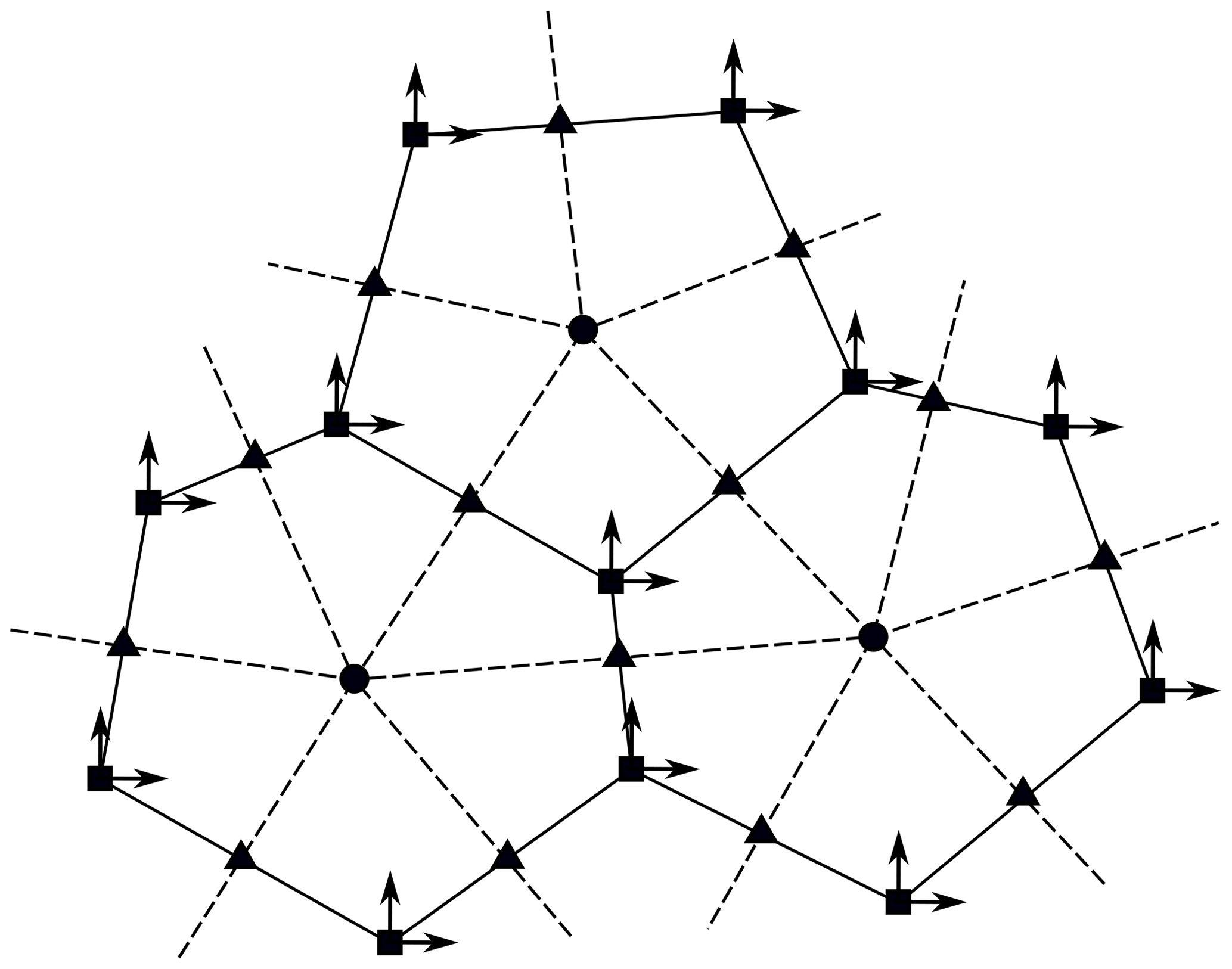
Figure 1Schematic representation of three cells in an example MPAS mesh. The mesh is composed of cell centers (circles), cell edge points (triangles), and cell vertices (squares). The dual triangular Delaunay mesh is formed by joining cell centers (dashed line). MPAS-Seaice uses a “B” type grid, with both velocity components defined at cell vertices. Unlike traditional quadrilateral meshes, the directions of the velocity components in MPAS-Seaice are not in general aligned with the cell edges.
2.2 Velocity solver
MPAS-Seaice uses a “B” Arakawa-type grid (Arakawa and Lamb, 1977) with both components of velocity defined at cell vertices and with sea-ice concentration, volume, and other tracers defined at cell centers (see Fig. 1). When using CICE-like quadrilateral meshes, the velocity solver algorithm of MPAS-Seaice reduces to that of CICE, allowing CICE and MPAS-Seaice to use identical test cases and supporting rapid testing and development of MPAS-Seaice.
In CICE the velocity components are aligned with the quadrilateral mesh. This is not possible, in general, with MPAS-Seaice since a SCVT MPAS mesh does not have edges with perpendicular directions as in a quadrilateral mesh. Instead, the velocity components at a given MPAS vertex are defined as eastwards (u) and northwards (v), irrespective of the orientation of edges joining that vertex. Such a definition, however, would result in a convergence of v components of velocity at the geographic poles and strong metric terms in the velocity solution. Consequently, we rotate the coordinate system so that the pole of u and v lies on the geographical Equator at 0∘ longitude. The polar regions then have the smallest metric effects on the globe.
To prognose sea-ice velocity we solve the same sea-ice momentum equation as CICE (Hibler, 1979; Hunke and Dukowicz, 1997):
Here m is the mass of snow and ice per unit area; u is the sea-ice velocity; σ is the ice internal stress tensor; τa and τw are the horizontal stresses due to atmospheric winds and ocean currents, respectively; is the unit vector normal to the Earth surface; f is the Coriolis parameter; g is the acceleration due to gravity; and Ho is the ocean surface height. The second-to-last term represents the Coriolis force, and the last term represents the force due to the ocean surface tilt. Only the internal stress divergence and ocean surface tilt terms depend on horizontal differential operators. During coupled simulations the ocean model provides the ocean surface tilt term, whereas in non-coupled simulations we assume that the ocean currents are in geostrophic balance so that
where uo is the geostrophic component of the ocean surface velocity. Consequently, only the internal stress divergence depends on the properties of the horizontal grid, and only adaptations to this stress term are required to adapt the velocity solver of CICE to MPAS meshes. The other terms in the momentum equation are solved in an identical way to CICE.
Determination of the divergence of the internal stress can be broken down into three stages:
-
Determine the strain rate tensor from the velocity field.
-
Determine the stress tensor at a point, through a constitutive relation, from the strain rate tensor at that point.
-
Calculate the divergence of this stress tensor.
As in CICE we use an elastic–viscous–plastic (EVP) rheology (Hunke and Dukowicz, 1997) for the constitutive relation. This step does not depend on the details of the horizontal mesh, and we use the same formulation as CICE. We develop two schemes to calculate the strain rate tensor and the divergence of internal stress on MPAS meshes. A variational scheme is based on that used in CICE (Hunke and Dukowicz, 2002), whereas a finite-volume scheme uses the line-integral forms of the symmetric gradient and divergence operators. These schemes are described in the following sections.
2.2.1 Variational scheme
We develop a variational scheme for calculating the stress divergence based on that of Hunke and Dukowicz (2002) but adapted for arbitrarily shaped and sided convex polygons. The principal change needed to adapt Hunke and Dukowicz (2002) to polygonal cells is a generalization of the basis functions from bilinear to a basis compatible with polygonal cells. The variational scheme is based on the fact that over the entire domain, Ω, the total work done by the internal stress is equal to the dissipation of mechanical energy:
Here is the strain rate tensor, and the integrals are area integrals over the whole model domain. For simplicity we ignore boundary effects, which would add additional terms to the right-hand side of this equation. The stress divergence operator is derived from the functional
where
In this functional the stress, σ, is taken as a separate parameter to the velocity, u. The derivation proceeds by determining a discretized version of the I[u,σ] functional and taking the variation of this functional with respect to one of the discretized velocities. The discretized functional is given by
where the functional has the discretized velocity components, ui and vi, and the discretized stresses, σj, as parameters; u is the eastwards component of u, while v is the northwards, and the two components of the stress divergence have been written as and . The work done in the whole domain has been split into a sum over the contributions to the work done in each cell () on the dual Delaunay mesh. The contribution to the work done in each dual cell is an area integral over each dual cell. These dual cells consist of either triangles (for SCVT meshes), or quadrilaterals (for quadrilateral meshes) surrounding a single primary mesh vertex point where the discretized velocity is defined. The dissipation of mechanical energy, D, has been written as a function of the discretized velocity components and discretized stresses. The simplest assumption for the velocity and stress divergence components for the work part of the discretized functional is that these quantities are constant within the dual cell. This is assumed by Hunke and Dukowicz (2002), but we later improve this assumption. With this initial assumption the discretized functional becomes
Taking the variation in this functional with respect to a single discretized velocity component, uj, we get the following Euler–Lagrange equation
where
and within the Euler–Lagrange equation. In the following the strain rate in D will be given directly in terms of ui and vi rather than and , so the second term of the Euler–Lagrange equation is zero. Then
and consequently the u component of the stress divergence for vertex j is given by
Fv is obtained in a similar way by taking the variation in I with respect to vj. The dissipation of mechanical energy, D, can be split into three terms:
with
We calculate the contribution to Fu and Fv from D1. Similar contributions come from D2 and D3. Using the expression for in terms of the velocity components and latitude θ, D1 becomes
where x and y are locally Cartesian coordinates, with x in the rotated eastwards direction and y in the rotated northwards direction, and r is the radius of the Earth. The second term in accounts for the metric effects of the curved domain (Batchelor, 1967). The integral can be broken up into a sum over the np cells in the primary mesh:
where the integral is over the interior area of the kth cell. To perform this integral we use a set of Lagrangian basis functions, 𝒲l, to represent functions within a cell of the primary mesh. These basis functions are such that if a function, ψ, has a value of ψl at vertex l of a cell, then the value of the function at a position (x,y) within the cell can be approximated as
where the sum is over the nv vertices of the cell in the primary mesh. Necessary properties for these basis functions are that
across the cell and that
We provide two options for the choice of basis functions, 𝒲l: Wachspress basis functions and piecewise linear (PWL) basis functions. Both basis functions have a value of one on vertex l and zero on the other vertices of a cell and are linear on the cell boundaries. The Wachspress basis function for the ith vertex of a polygon with n sides is given by (Dasgupta, 2003)
where
and
lj(x,y) is the line equation for the j polygon edge such that
where aj and bj are defined by the condition that along the jth edge of the polygon. When written out, 𝒲i becomes a rational polynomial of the form
where 𝒫(m)(x,y) is an m-degree polynomial in x,y. The integrals of the Wachspress basis function within a cell are performed using the eighth-order quadrature rules of Dunavant (1985). For quadrilateral meshes the Wachspress basis functions reduce to the bilinear basis functions used in CICE. For the four vertices of the quadrilateral cells, these are given by
where ξ1 and ξ2 are the transformed unit square coordinates of the cell (Hunke, 2001).
PWL basis functions divide the polygonal cell into sub-triangles and use a linear basis within each sub-triangle (Bailey et al., 2008). To divide the polygonal cell into sub-triangles, a point is chosen within the cell and sub-triangles formed using this point and two adjacent vertices. The central point in the cell, xc, is chosen as
where the sum is over the nv vertices of the cell each with position xi. The simplest choice for the αi is to set them all equal to the inverse of the number of cell vertices, . Example basis functions for the Wachspress and PWL basis functions are shown in Fig. 2.
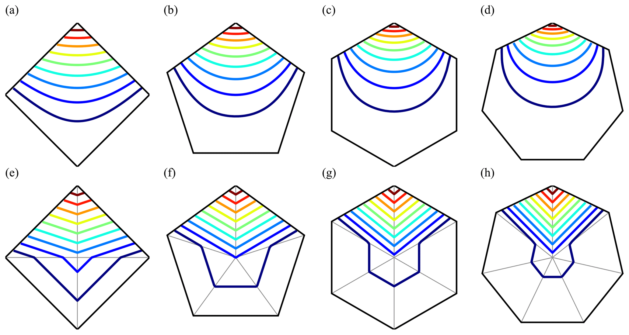
Figure 2Example basis functions for the (a–d) Wachspress and (e–h) PWL methods. The basis function is shown for the top vertex for a (a, e) square, (b, f) pentagonal, (c, g) hexagonal, and (d, h) heptagonal cell. Contour levels are drawn between 0.1 (dark blue) and 0.9 (red) at intervals of 0.1.
Using those basis functions to expand σ11 (with basis index l), u, and v (with basis index m), Eq. (15) can be written as
where the derivative with respect to x has been taken inside the summation. Rearranging, this becomes
In moving the integral, we have assumed that θ, the latitude, is constant in the cell. The terms involving integrals are now only a function of the geometry of the mesh and can be calculated once for each cell during the initialization phase of the model run. Defining
and
we have
Taking the variation with respect to a discretized velocity component at a particular vertex point, j, as in Eq. (11), now gives us the contribution from D1 to the components of the stress divergence tensor at that velocity point:
Only cells that border the vertex point j contribute to the k sum over cells. The total stress divergence at the point j is then the sum of the contributions from D1, D2, and D3:
All that remains is to determine the stress for each cell at its vertices. As in the formulation in CICE, each cell has its own stress value at its vertices, so each vertex has several values of the stress, each corresponding to a different surrounding cell. The stresses are calculated from the strain rate tensor at each vertex using the constitutive relation (see Sect. 2a of Hunke and Dukowicz, 2002). Including metric effects (Batchelor, 1967), the strain rate tensor is given by
The strain rate tensor at cell vertex l is then given by
The derivatives of the basis functions are taken at cell vertex l. For the variational method pre-computed values for the variables , , 𝒯lm, , and must be stored, resulting in a total of values stored per cell.
One issue with the above derivation is the ambiguity of defining the correct dual cell area, Aj, for Eq. (11) since the cell center positions do not appear anywhere else in the formulation. In Sect. 3.1.2, in a unit sphere test case with analytical input stress fields, it is evident that using the default MPAS dual cell area for Aj results in large errors in the calculated stress divergence field around the 12 pentagonal cells found on a quasi-uniform SCVT mesh. An alternative to using the MPAS dual cell area and assuming constant stress and velocity within a dual cell for the work equation is to assume that the velocity and divergence are given by the same basis functions as used for the dissipation of mechanical energy. Then the work done over the domain
Taking the variation in I with respect to the discretized velocity component uj
where the sum over i cells is reduced to those surrounding the j vertex. This generates an undesirable implicit problem necessitating a global matrix inversion, which can be avoided if the stress divergence varies slowly spatially. This is the equivalent of lumping the mass matrix in the finite element method (Reddy, 1993). Then
where the sum over m is over the vertices in each cell surrounding the j vertex. This suggests an alternative to Aj given by
We find that approximating Aj with reduces the error in the stress divergence operator as compared to using the standard dual mesh areas and requires no additional calculations of integrals at initialization.
2.2.2 Finite-volume scheme
An alternative method of deriving operators is with an integral method where the divergence theorem is used to equate the integral form of the operator to a flux integrated around a closed loop. One potential advantage of the finite-volume scheme is that it solves the conservative form of the momentum equation and can handle non-smooth solution features (such as sharp fronts) consistently.
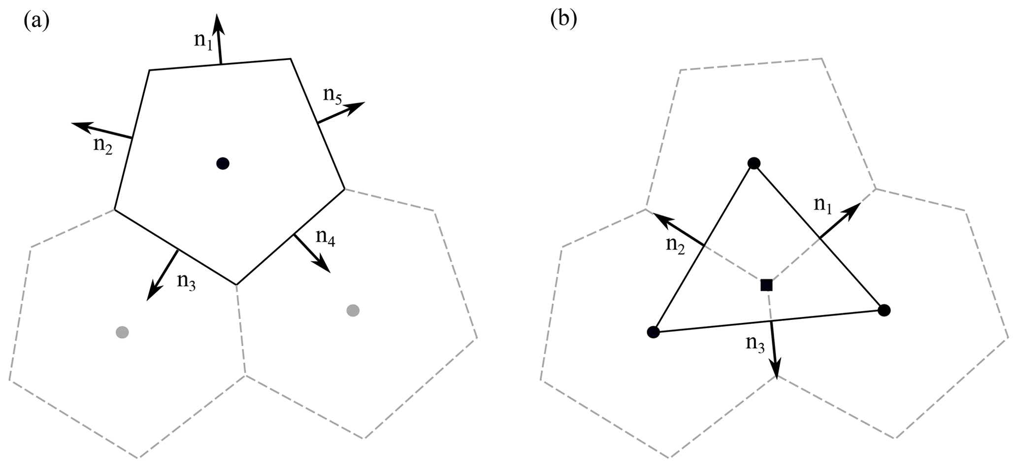
Figure 3Contour integration lines used by the finite-volume stress divergence operator scheme. (a) Strain rate at cell centers (circle) are calculated from line integrals around primary mesh cells (solid line). (b) Stress divergence at cell vertices (square) are calculated from line integrals around the dual mesh cells (solid line). Directions of normal vectors used in the integrals are shown for both panels.
For the finite-volume scheme we use line integrals around cells in the primary and dual meshes to calculate the strain rate tensor and the stress divergence, respectively. To determine the strain rate tensor we start from the generalized divergence theorem
where n is the normal to the closed surface S of domain Ω, and ⊗ is the tensor product. The symmetric version of this operator is then obtained as
The strain rate at a point is then obtained from the limit
where the integral is around a closed loop, S, with area A and normal vector n, and v is the sea-ice velocity. To determine the strain rate tensor at the centers of the primary mesh, we take this integral around the edges of the cells in the primary mesh. First the cell is projected onto a flat tangent plane perpendicular to the vector joining the center of the sphere to the cell center. We take the sea-ice velocity at a cell edge as the average of the values on the two vertices forming that edge projected onto the tangent plane:
Here, A is the area of the primary cell, the summation is over the ne edges of the primary cell, ni is the normal vector to the edge i that lies in the tangent plane, vi is the edge velocity, and li is the length of edge i. We use the tangential projection of the velocity and account for metric terms separately. The full strain rate tensor including these metric terms is (Batchelor, 1967)
where the prime symbol signifies a strain rate without metric terms. The stress, which is determined from the strain rate tensor using the constitutive relation, is now defined on cell centers. To find its divergence we use the divergence theorem
or
for the stress divergence at a point. The divergence of internal stress is determined at primary cell vertices (where the velocity is defined and momentum equation solved) by performing a sum around the edges of the dual mesh on a tangent projected plane, tangential to the primary cell vertex. The vertices of the dual mesh are the cell centers of the primary mesh where the strain rate has been determined. The stress divergence at primary cell vertices is then given by
where Ad is the area of the dual mesh cell, the sum is over the nc vertices of the dual mesh, li is the length of the i edge of the dual mesh, and ni is a normal vector to the i edge on the projected plane. Metric terms in the divergence of a second-order tensor, like the stress tensor, have two contributions: the first comes from the varying grid cell size and the second from the varying directions of the coordinate basis vectors (Malvern, 1969). Equation (45) accounts for the first of these effects, and in order to account for the second effect the stress divergence becomes
where the components of σ are approximated as the average of the values on the dual mesh vertices.
2.3 Transport
To transport sea-ice fractional area and various tracers, MPAS-Seaice uses an incremental remapping (IR) algorithm similar to that described by Dukowicz and Baumgardner (2000), Lipscomb and Hunke (2004), and Lipscomb and Ringler (2005). The Lipscomb and Hunke (2004) scheme was designed for structured quadrilateral meshes and is implemented in CICE (Hunke et al., 2015). The Lipscomb and Ringler (2005) scheme was implemented on a structured SCVT global mesh consisting of quasi-regular hexagons and 12 pentagons.
For MPAS-Seaice the IR scheme was generalized to work on either the standard MPAS mesh (hexagons and other n-gons of varying sizes, with a vertex degree of 3 as in Lipscomb and Ringler, 2005) or a quadrilateral mesh (with a vertex degree of 4 as in Lipscomb and Hunke, 2004, and CICE). Since the CICE IR transport code assumes a structured mesh, but MPAS meshes are unstructured, the IR scheme had to be rewritten from scratch. Most of the MPAS-Seaice IR code is now mesh-agnostic, but a small amount of code is specific to quad meshes as noted below.
Here we review the conceptual framework of incremental remapping as in Hunke et al. (2015) and describe features specific to the MPAS-Seaice implementation. IR is designed to solve equations of the form
where is the horizontal velocity; m is mass or a mass-like field (such as density or fractional sea-ice concentration); and T1, T2, and T3 are tracers. These equations describe conservation of quantities such as mass and internal energy under horizontal transport. Sources and sinks of mass and tracers (e.g., ice growth and melting) are treated separately from transport.
In MPAS-Seaice, the fractional ice area in each thickness category is a mass-like field whose transport is described by Eq. (47). (Henceforth, “area” refers to fractional ice area unless stated otherwise.) Ice and snow thickness, among other fields, are type 1 tracers obeying equations of the form of Eq. (48), and the ice and snow enthalpy in each vertical layer are type 2 tracers obeying equations like Eq. (49), with ice or snow thickness as their parent tracer. When run with advanced options (e.g., active melt ponds and biogeochemistry (BGC)), MPAS-Seaice advects tracers up to type 3. Thus, the mass-like field is the “parent field” for type 1 tracers, type 1 tracers are parents of type 2, and type 2 tracers are parents of type 3.
Incremental remapping has several desirable properties for sea-ice modeling:
-
It is conservative to within machine roundoff.
-
It preserves tracer monotonicity. That is, transport produces no new local extrema in fields like ice thickness or internal energy.
-
The reconstructed mass and tracer fields vary linearly in x and y. This means that remapping is second-order accurate in space, except where gradients are limited locally to preserve monotonicity.
-
There are economies of scale. Transporting a single field is fairly expensive, but additional tracers have a low marginal cost, especially when all tracers are transported with a single velocity field as in CICE and MPAS-Seaice.
The time step is limited by the requirement that trajectories projected backward from vertices are confined to the cells sharing the vertex (i.e., three cells for the standard MPAS mesh and four for the quad mesh). This is what is meant by incremental as opposed to general remapping. This requirement leads to a Courant–Friedrichs–Lewy (CFL)-like condition,
where Δx is the grid spacing, and Δt is the time step. For highly divergent velocity fields, the maximum time step may have to be reduced by a factor of 2 to ensure that trajectories do not cross.
The IR algorithm consists of the following steps:
-
Given mean values of the ice area and tracer fields in each grid cell and thickness category, construct linear approximations of these fields. Limit the field gradients to preserve monotonicity.
-
Given ice velocities at grid cell vertices, identify departure regions for the transport across each cell edge. Divide these departure regions into triangles, and compute the coordinates of the triangle vertices.
-
Integrate the area and tracer fields over the departure triangles to obtain the area, volume, and other conserved quantities transported across each cell edge.
-
Given these transports, update the area and tracers.
Since all fields are transported by the same velocity field, the second step is done only once per time step. The other steps are repeated for each field.
With advanced physics and BGC options, MPAS-Seaice can be configured to include up to ∼ 40 tracer fields, each of which is advected in every thickness category and many of which are defined in each vertical ice or snow layer. In order to accommodate different tracer combinations and make it easy to add new tracers, the tracer fields are organized in a linked list that depends on which physics and BGC packages are active. The list is arranged with fractional ice area first, followed by the type 1 tracers, type 2 tracers, and finally type 3 tracers. In this way, values computed for parent tracers are always available when needed for computations involving child tracers.
The MPAS-Seaice version of the incremental remapping transport scheme has several advantages over the one in CICE. First, as already mentioned, the scheme has been generalized to work for SCVT as well as quadrilateral meshes. Second, the MPAS-Seaice scheme treats T3 tracers more accurately by using more accurate integration formulas (see Eq. 60).
We next describe the IR algorithm in detail, pointing out features that are new in MPAS-Seaice.
2.3.1 Reconstructing area and tracer fields
The fractional ice area and all tracers are reconstructed in each grid cell (quadrilaterals, hexagons, or other n-gons) as functions of in a cell-based coordinate system. On spherical grids, r lies in a local plane that is tangent to the sphere at the Voronoi cell center. The state variable for ice area, denoted as , should be recovered as the mean value when integrated over the cell:
where AC is the grid cell area. Equation (52) is satisfied if a(r) has the form
where ∇a is a cell-centered gradient, αa is a coefficient between 0 and 1 that enforces monotonicity, and is the cell centroid:
Similarly, tracer means should be recovered when integrated over a cell:
These equations are satisfied when the tracers are reconstructed as
where the tracer barycenter coordinates are given by
The integrals in Eq. (57) can be evaluated by applying quadrature rules for linear, quadratic, and cubic polynomials as described in Sect. 2.3.3.
Monotonicity is enforced by van Leer limiting (van Leer, 1979). The reconstructed area and tracers are evaluated at cell vertices, and the coefficients α are reduced as needed so that the reconstructed values lie within the range of the mean values in the cell and its neighbors. When α=1, the reconstruction is second-order accurate in space. When α=0, the reconstruction reduces locally to first-order.
2.3.2 Locating departure triangles
The next step is to identify the departure region associated with fluxes across each cell edge and to divide the departure region into triangles. Figure 4a illustrates the geometry for the standard MPAS mesh. The edge has vertices V1 and V2. Each edge is oriented such that one adjacent cell (C1) is defined to lie in the left half-plane and the other (C2) in the right half-plane. The departure points D1 and D2 are found by projecting velocities backward from V1 and V2. The shaded departure region is a quadrilateral containing all the ice transported across the edge in one time step. In addition to C1 and C2, the departure region can include side cells C3 and C4. The side cells share edges E1 to E4 and vertices V3 to V6 with the central cells C1 and C2.
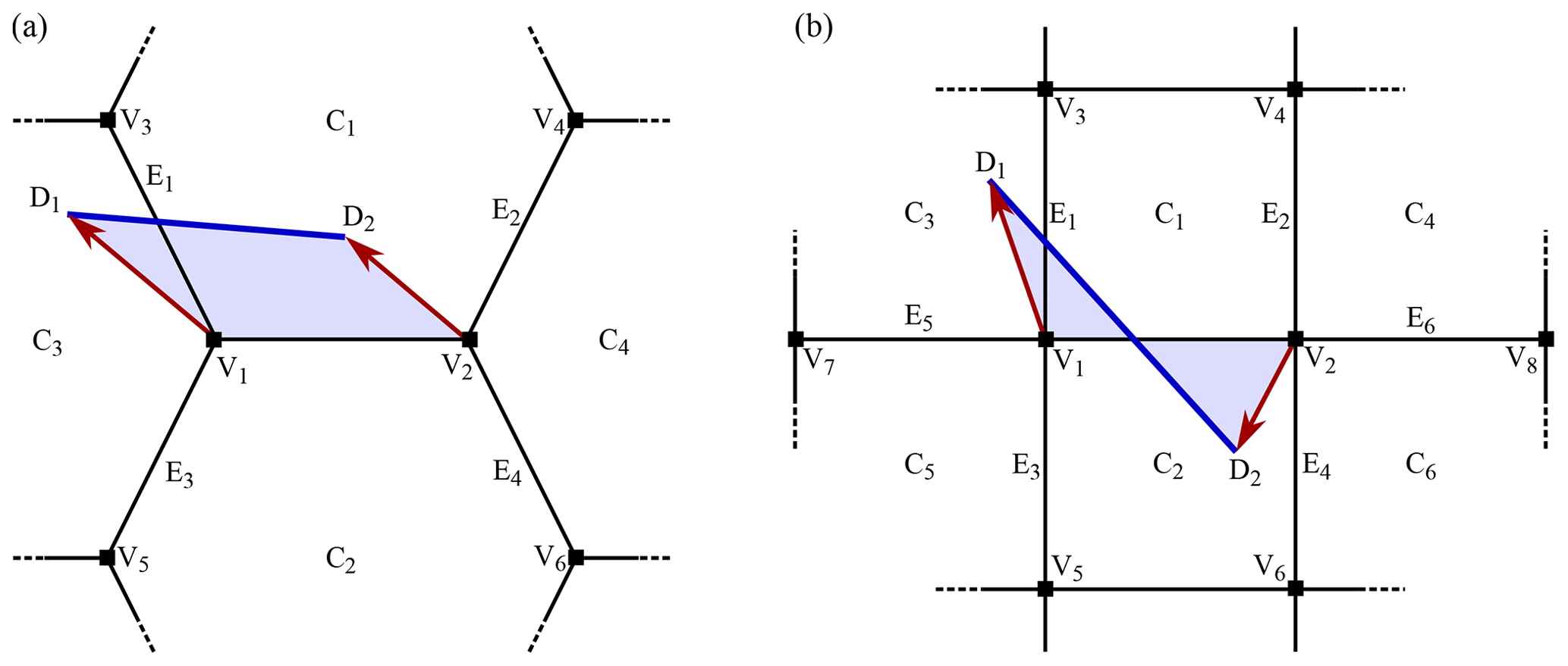
Figure 4(a) Schematic showing transport across a cell edge on a standard MPAS mesh with three edges meeting at each vertex. The letters C, E, and V denote cell centers, edges, and vertices, respectively. Vertices are also shown with a square marker. Backward trajectories are shown as red arrows, ending in departure points D1 and D2. These backward trajectories define the departure region, which is shaded in blue. (b) Schematic showing transport across a cell edge on a quadrilateral MPAS mesh with four edges meeting at each vertex. Shaded regions are the departure regions.
The edges and vertices in Fig. 4a are defined in a coordinate system lying in the local tangent plane at the midpoint of the main edge, halfway between V1 and V2. These coordinates are pre-computed at initialization. During each time step, departure triangles are found by locating D1 and D2 in this coordinate system and then looping through the edges to identify any intersections of line segment (i.e., the segment joining D1 and D2) with the various edges. If intersects the main edge, then the departure region consists of two triangles (one each in C1 and C2) rather than a quadrilateral (as shown in Fig. 4b). If intersects any of edges E1 to E4, the departure region includes triangles in side cells.
Each departure triangle lies in a single grid cell, and there are at most four such triangles. There are two triangles in the central cells (either one each in C1 and C2 or a quadrilateral that can be split into two triangles) and up to two triangles in side cells. The triangle vertices are a combination of cell vertices (V1 and V2), departure points (D1 and D2), and intersection points (points where crosses an edge).
Figure 4b shows the geometry for a quadrilateral mesh. In this figure the departure region consists of two triangles, but it could also be a quadrilateral as in Fig. 4a. For the quad mesh there are two additional side cells (C5 and C6), edges (E5 and E6), and vertices (V7 and V8). The search algorithm is designed such that the code used to find departure triangles for the standard mesh is also applied to the quad mesh. For quad meshes only, there is additional logic to find intersection points and triangles associated with the extra edges and cells. This is the only mesh-specific code in the runtime IR code. For the quad mesh there are at most six departure triangles: two in the central cells and one in each of the four side cells. If the edges meet at right angles as shown in the figure, the maximum is five triangles, but this is not a mesh requirement.
Once triangle vertices have been found in edge-based coordinates, they are transformed to cell-based coordinates, i.e., coordinates in the local tangent plane of the cell containing each triangle. (Coefficients for these transformations are computed at initialization.) Triangle areas are computed as
where the (xi,yi) are the triangle vertices.
2.3.3 Integrating the transport
Next, ice area and area-tracer products are integrated in each triangle. The integrals have the form of Eq. (52) for area and Eq. (55) for tracers. Since each field is a linear function of (x,y) as in Eqs. (53) and (56), the area-tracer products are quadratic, cubic, and quartic polynomials, respectively, for tracers of type 1, 2, and 3.
The integrals can be evaluated exactly by summing over values at quadrature points in each triangle. Polynomials of quadratic or lower order are integrated using the formula
The quadrature points are located at , where x0 is the triangle midpoint, and xi are the three vertices. The products involving type 2 and type 3 tracers are cubic and quadratic polynomials, which can be evaluated using a similar formula with six quadrature points:
where x1i and x2i are two sets of three quadrature points, arranged symmetrically on the three medians of the triangle, and w1 and w2 are weighting factors. Coefficients and weighting factors for these and other symmetric quadrature rules for triangles were computed by Dunavant (1985). These integrals are computed for each triangle and summed over edges to give fluxes of ice area and area-tracer products across each edge.
2.3.4 Updating area and tracer fields
The area transported across edge k for a given cell can be denoted as Δak and the area-tracer products as Δ(aT1)k, Δ(aT1T2)k, and Δ(aT1T2T3)k. The new ice area at time n+1 is given by
where the sum is taken over cell edges k, with a positive sign denoting transport into a cell and a negative sign denoting outward transport. The new tracers are given by
Dukowicz and Baumgardner (2000) showed that Eq. (62) satisfies tracer monotonicity since the new-time tracer values are area-weighted averages of old-time values.
2.4 Column physics
CICE has sophisticated vertical physics and biogeochemical schemes, which include vertical thermodynamics schemes (Bitz and Lipscomb, 1999; Turner et al., 2013; Turner and Hunke, 2015), several melt-pond parameterizations (Flocco et al., 2010; Holland et al., 2012; Hunke et al., 2013), a delta-Eddington radiation scheme (Briegleb and Light, 2007; Holland et al., 2012), schemes for transport in thickness space (Lipscomb, 2001), representations of mechanical redistribution (Lipscomb et al., 2007), and sea-ice BGC (Jeffery and Hunke, 2014; Jeffery et al., 2016, 2020). To include these developments in MPAS-Seaice, the column physics and BGC in CICE have been extracted into a separate library, which performs column calculations on individual grid cells with no knowledge of the details of the horizontal mesh used by the host model. This column package, now called Icepack, is used by the most recent version of CICE (Hunke et al., 2018). MPAS-Seaice uses a version of the column package that was forked from CICE version 5.1.2.
3.1 Velocity solver
To validate our implementation of the MPAS-Seaice velocity solver we investigate several idealized test cases.
3.1.1 Operators on planar meshes
In the first test case, we define analytical test fields on a unit square planar mesh with regularly shaped cells and determine the error generated by the strain and stress divergence operators when acting on these fields. Since the strain rate operators consist of a combination of spatial derivatives in the x and y directions, we examine the error generated by these spatial derivative operators instead of directly by the strain rate operator. We examine meshes with both square and hexagonal cells. The test analytical field for which spatial derivatives are calculated is given by
with A=2.56. This field gives sufficient variation to provide an adequate test of the operators, while the symmetry of f(x,y) between the x and y directions allows an accurate comparison between the and operators. Figure 5 shows the scaling of the L2 error norm for the spatial derivatives against grid resolution. For the spatial derivatives examined in this section and the strain rates examined in Sect. 3.1.2, we calculate the L2 norm with the following methods. For the variational operators we integrate the square of the error across the domain using the variational basis functions defined in Sect. 2.2.1 for the quantity of interest. The L2 norms for the variational derivatives and strains are given by
where the sum over i is a sum over cells in the region of interest, and the area integral is over cell i, performed by splitting the polygon into sub-triangles and using the eighth-order integration rules of Dunavant (1985). The modeled quantity of interest is determined within the interior of the cell from the basis functions, 𝒲l, and quantity of interest, fil, on vertex l of cell i. For strains calculated with the Wachspress basis function we perform the integration with the Wachspress basis functions and likewise for the PWL basis functions; represents the analytical values of the field of interest within the cell. For the finite-volume strain operators we perform line integrals of the square of the error around the dual mesh cell surrounding primary cell points. The L2 norms for the finite-volume derivatives and strains are given by
where the sum i is over the primary cells, and the sum j is over the edges of the dual cell surrounding cell i. Coordinate χ signifies the position along edge j, with fj(χ) calculated from a linear interpolation from the strain values at each end of the edge; are the analytical values of the field of interest along the edge. The line integrals are performed with seventh-order Gauss–Lobatto quadrature rules. These formulas emulate how the stress values, derived from the strain values, are used in their respective stress divergence operators. Each doubling of resolution should reduce the L2 error norm by a factor of 2 for first-order accurate schemes and a factor of 4 for second-order accurate schemes. Figure 5 also shows idealized first- and second-order scaling gradients as dotted lines. Evident from the figure is that the spatial derivative operators for the variational methods (Wachspress and PWL) are only first-order accurate for both square and hexagonal meshes, while the finite-volume derivative operators are second-order accurate with much lower errors than the variational methods. This is understandable since the variational derivative operators only use velocity values from vertices on the same cell as the vertex that the derivative is being calculated for. These velocity values can then only occupy one half-plane with respect to the derivative point, effectively creating a one-sided stencil for the operator. Velocity values for the finite-volume operator, however, surround the derivative point since here the derivative point is at the center not the side of the cell. This effectively creates a stencil surrounding the derivative location. Small differences exist between the Wachspress and PWL variational basis functions as well. Differences between errors generated for the x and y spatial derivatives are evident for the hexagonal mesh. These differences are caused by a difference in spatial symmetry of the mesh in these two directions for the hexagonal mesh, whereas the square mesh has the same spatial symmetry in both directions. These results are confirmed by an error analysis with a Taylor series expansion of the methods. One possible way to improve the accuracy of the variational operators is to average for each surrounding cell the different one-sided values of the derivatives calculated for a single vertex to create a multi-sided stenciled operator from the one-sided variational ones. Figure 5 shows the error scaling for this averaging method for the Wachspress (“Wachs. Avg”) and PWL (“PWL Avg”) basis functions. Second-order convergence is achieved in the y direction with this averaging, but interestingly, only averaging the PWL basis function results in second-order convergence in the x direction, while the Wachspress basis function shows only first-order convergence with much larger errors in the x direction. This difference between the two directions is explained by the different geometric symmetry found in the two directions, with, for this test case, the x direction parallel to a line from a cell center to a vertex and the y direction parallel to a line from a cell center to edge center. The derivatives at cell centers calculated by the finite-volume method can also be averaged to the cell vertices to create another operator (“FV Avg” in Fig. 5), creating a second-order accurate method, although this averaging increases the error relative to the original finite-volume scheme.
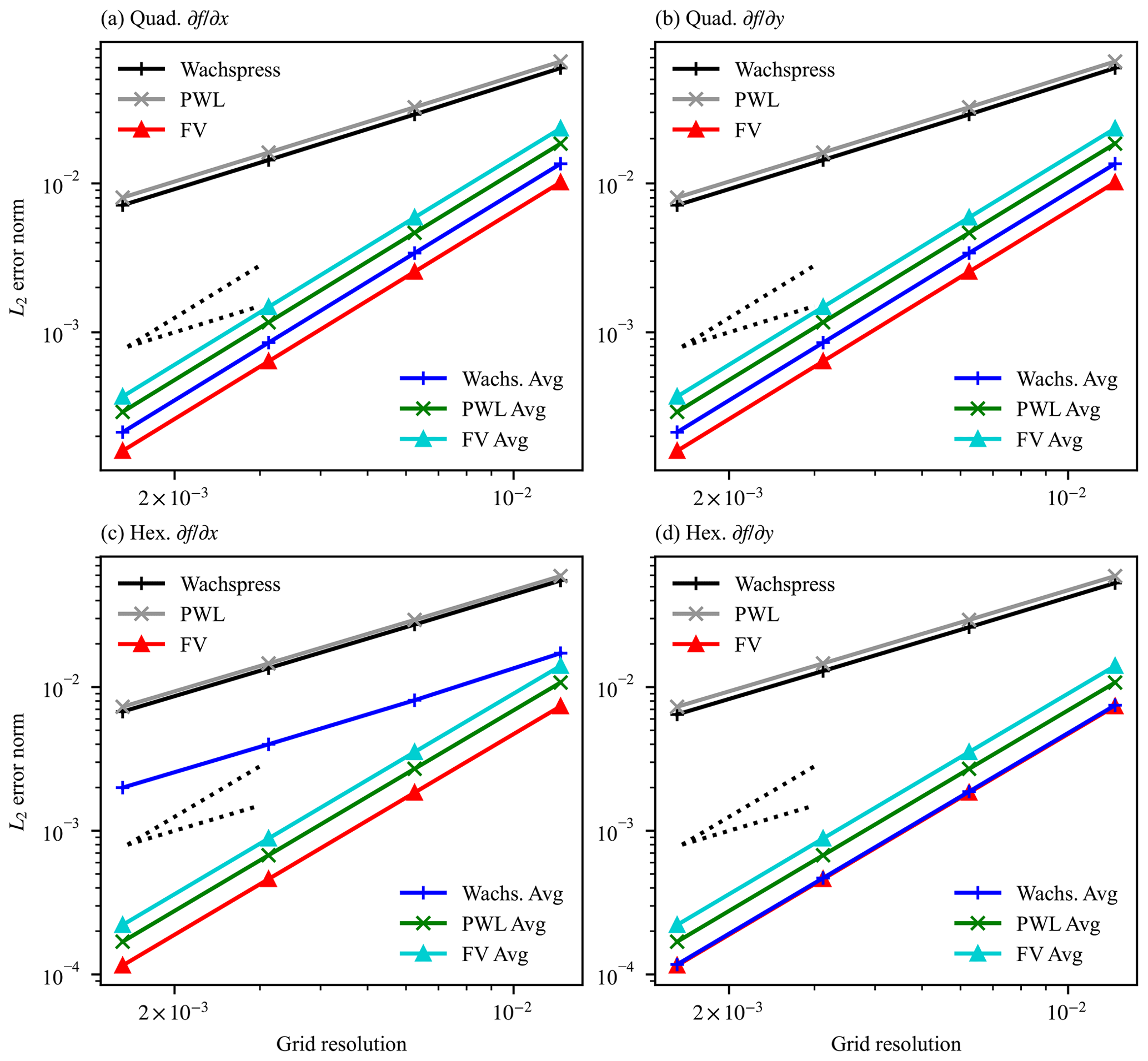
Figure 5Scaling of L2 error norm against grid resolution for the model calculation of the gradient of an analytical function in the (a, c) x and (b, d) y directions for a planar test case with a regular (a, b) square cell and (c, d) hexagonal cell mesh. Grid resolution is the mean distance between cell centers. Ideal first- and second-order scaling gradients are also shown as dotted lines.
Next, with the same meshes we examine the error scaling of the stress divergence operator. The same function as above, f(x,y), is used for the u and v components of velocity, and the analytical strain rates are calculated from these velocity components. The analytical internal ice stresses and stress divergence are calculated from this strain rate assuming a linear constitutive relation of the form . The analytical internal stresses are used as input to the stress divergence operators, and the output is compared to the analytical stress divergence. Figure 6 shows the scaling of the L2 error norm of the stress divergence operators with grid resolution. For the L2 error norm calculated for the stress divergence operators in this section and in Sect. 3.1.2, we use
where the sum is over either grid cells or vertices in the region of interest; Ai is the area of either the primary cell or the dual cell surrounding the vertex; and fi and are the model and analytical values of the field of interest, respectively. Both the variational and finite-volume methods show second-order convergence of errors for the square cell mesh, with the finite-volume scheme showing significantly lower errors. With the PWL basis functions the variational method shows second-order convergence, while with Wachspress basis functions the variational method shows a varying order of convergence with near-second-order convergence at low resolution but with the order decreasing to first with higher resolutions. This suggests there is a small source of first-order error when using the Wachspress basis functions. For the hexagonal cell mesh, the finite-volume method shows only first-order convergence with significantly higher error than the variational method. This is because the line integral around vertices for the finite-volume method involves an integral around a triangle. Unlike the integral around a square or hexagon, there are no opposite sides to a triangle. For the finite-volume integrals around squares or hexagons, opposite edges of the polygon lead to cancellation of first-order error, which does not occur for integrals around triangles. Smaller differences between the x and y directions are visible than with the spatial derivative operators examined above. Again, these results are confirmed with a Taylor series expansion of the methods.
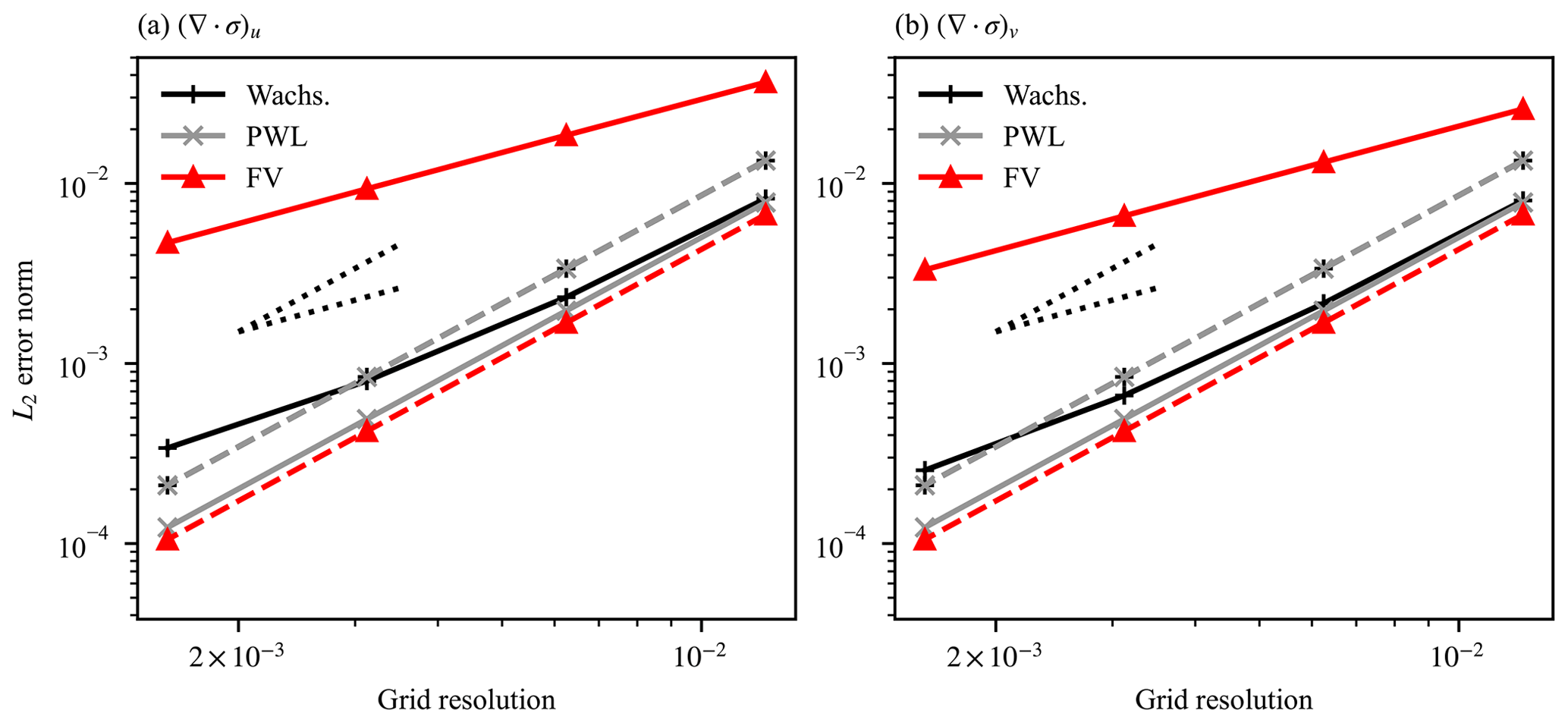
Figure 6Scaling of L2 error norm against grid resolution for the model calculation of the (a) u and (b) v components of stress divergence from an analytical strain rate tensor field for a planar test case with a regular mesh. Grid resolution is the mean distance between cell centers. Solid lines denote hexagonal cell meshes, whereas dashed lines signify square cell meshes. Ideal first- and second-order scaling gradients are also shown as dotted lines.
In summary, for regular planar meshes, for the gradient operators, the finite-volume and averaged PWL and averaged finite-volume schemes show a higher order of error convergence and lower absolute errors than the variational schemes, while the averaged Wachspress scheme shows a higher order of convergence than the unaveraged Wachspress scheme, except for hexagonal cell meshes when the x derivative is being calculated. Conversely, for the stress divergence operator and hexagonal cell meshes, the variational schemes show lower absolute errors and better error convergence than the finite-volume scheme, while for square cell meshes the order of convergence is the same between the variational and finite-volume schemes, with the finite-volume scheme producing lower absolute errors. Within the variational scheme, use of the PWL basis functions displays more consistent error convergence characteristics than the Wachspress scheme.
3.1.2 Operators on a unit sphere
Having examined the spatial operators on planar meshes, we now examine the effect of metric terms introduced by using the operators on a sphere. To do this we assume an analytical velocity field on a unit sphere and derive analytical strain rate and stress divergence fields from those velocity fields (again assuming a linear constitutive relation of the form ). We use spherical harmonic functions, Y, for the analytical velocity fields with and , where u, v, the latitude (θ), and the longitude (ϕ) are on the rotated geographical mesh (see Sect. 2.1). This choice of spherical harmonic, with different values of m and l for u and v, produces a sufficiently varying velocity field to test the strain rate and stress divergence operators. Figure 7a and b show these analytical velocity fields, while Fig. 7c and d and e, f, and g show the derived analytical fields for stress divergence and strain rate, respectively.
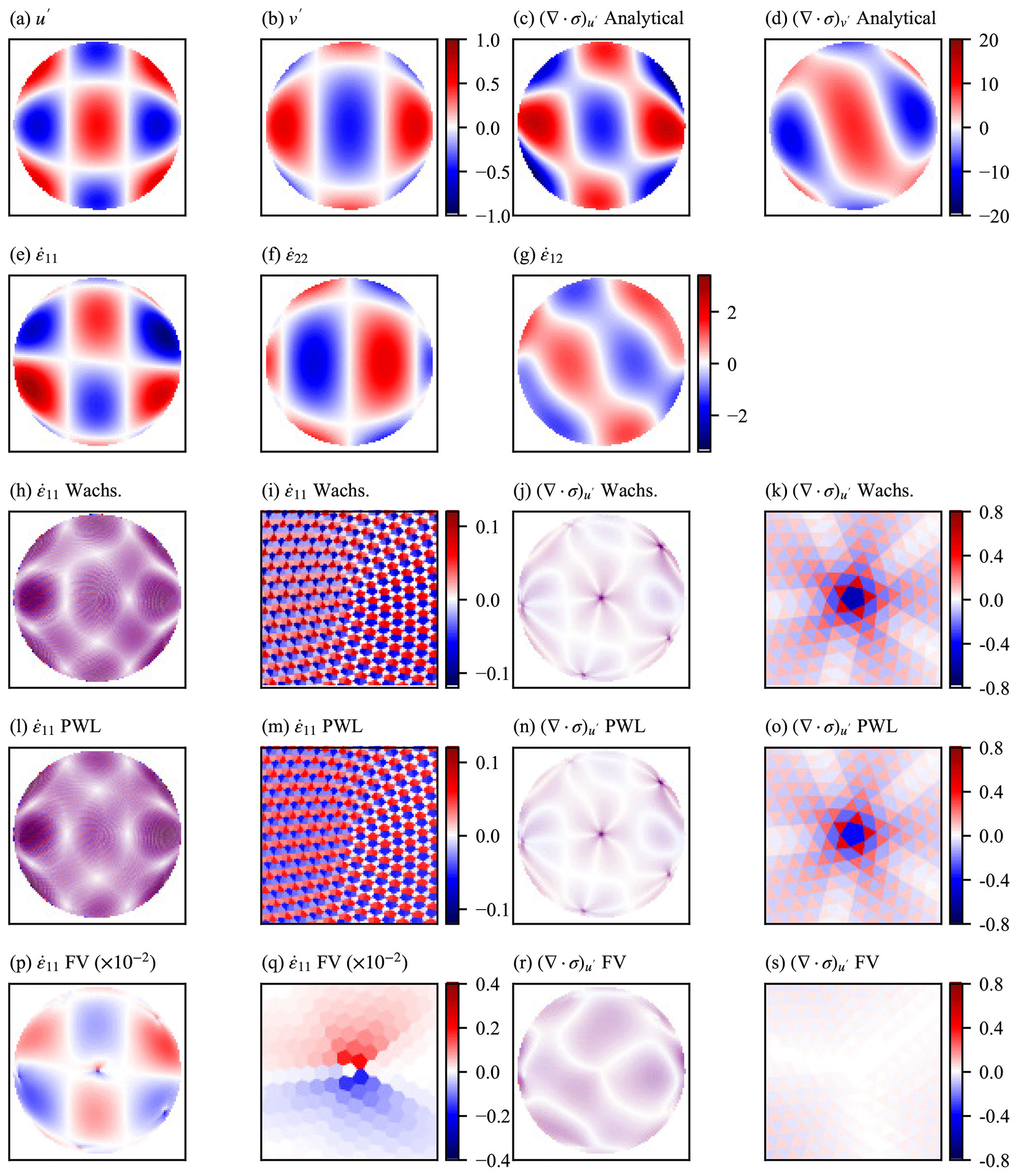
Figure 7Orthographic projection of one hemisphere of the unit sphere test case described in Sect. 3.1.2. Panels (a) and (b) show the analytical forms of velocity used in the numerical schemes and used to calculate the desired analytical strain rates (shown in e–g) and the desired analytical stress divergence (shown in c and d). Panels (h), (i), (l), (m), (p), and (q) show the error in calculation of the component of the strain rate for the (h, i) Wachspress variational scheme, the (l, m) PWL variational scheme, and the (p, q) finite-volume (FV) scheme. Panels (j), (k), (n), (o), (r), and (s) show the error in calculation of the u component of the stress divergence for the (j, k) Wachspress variational scheme, the (n, o) PWL variational scheme, and the (r, s) finite-volume (FV) scheme. Detail is shown around one of the pentagonal mesh cells for each scheme in (i), (k), (m), (o), (q), and (s). The error is the difference between the model and analytical values.
Errors generated for the strain rate component for this test case are displayed in Fig. 7h, l, and p. These show that the error is significantly lower for the finite-volume scheme compared to the two variational schemes. They also show that the error in the variational scheme consists of alternating signed error values within a cell, while the error for the finite-volume scheme is enhanced around the 12 pentagonal cells found in the quasi-uniform SCVT mesh. These features are clearer in Fig. 7i, m, and q, which show the detail around one of the pentagonal cells. A histogram of error values for the various strain rate operators is presented in Fig. 8a. Evident are the much larger error values for the variational schemes compared to the finite-volume scheme. The scaling of L2 error norm with grid resolution is shown in Fig. 9a. L2 error norm is calculated for regions of the grid with latitude (so that the poles of the rotated mesh are excluded) for four different grid resolutions. Evident from the scaling figure is that the variational schemes display first-order convergence, and the finite-volume scheme shows second-order convergence and much lower error levels. Also shown in this figure are results for the operator averaging methods described in Sect. 3.1.1. Here the PWL and finite-volume operator averaging show similar error scaling characteristics with close-to-second-order convergence. Also apparent is that a lower improvement in error for the Wachspress variational scheme is achieved with averaging, where convergence is closer to first order. Figure 9c shows the scaling of the L∞ norm, defined as , which shows first-order convergence for all strain rate operator methods. As for the hexagonal cell planar mesh, for both the L2 and L∞ norms, averaging the finite-volume scheme increases the error.
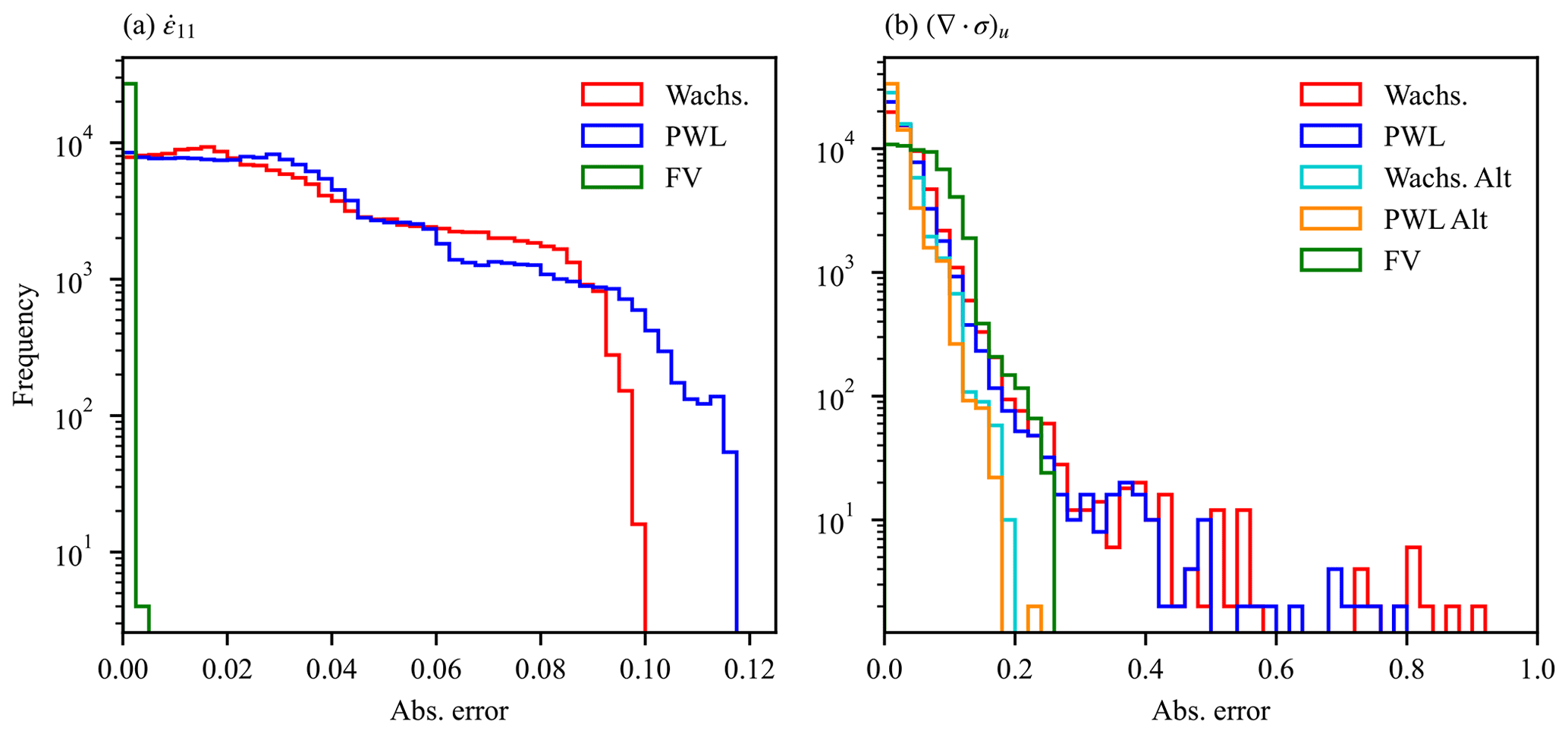
Figure 8Frequency of grid cell error in the calculation of strain rate (a) and stress divergence (b) from an analytical velocity field for a spherical test case. The error is given as the absolute value of the difference between model and analytical fields. The results are plotted as histograms for the two variational schemes (using Wachspress and PWL basis functions and the alternative area formulation) and the finite-volume (FV) scheme.
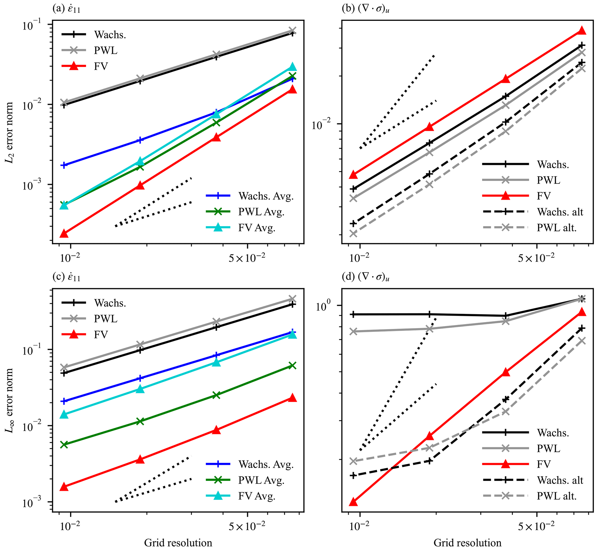
Figure 9Scaling of L2 (a, b) and L∞ (c, d) error norm against grid resolution for the model calculation of (a, c) the component of the strain rate tensor from an analytical velocity field and (b, d) the u component of the stress divergence from an analytical strain rate tensor field on the unit sphere for a spherical test case. Grid resolution is the mean distance between cell centers. Only mesh cells where are included. Ideal first- and second-order scaling gradients are also shown as dotted lines.
Next we examine the stress divergence operators on the unit sphere. Figure 7j, n, and r show the error for the two variational schemes and the finite-volume scheme. Away from the pentagonal cells, the variational methods display smaller errors than the finite-volume scheme but show a significant enhancement of error at the pentagonal cells, something not found with the finite-volume scheme. As for the strain rate operator, the two variational stress divergence schemes show very similar error patterns on the unit sphere. These results are more easily seen in Fig. 7k, o, and s, which again show the detail around one of the pentagonal cells. The error enhancement around the pentagonal cell is almost entirely due to the choice of area denominator in Eq. (11). For the area denominator Fig. 7 uses the triangle area of the dual cell. Figure 10 again shows the error for the stress divergence operator on the unit sphere for the two variational schemes, but using the alternate formulation for the area denominator defined in Eq. (37). As can be seen with this alternate formulation there is no enhancement in error around the pentagonal cells. Figure 8b shows a histogram of the errors generated by the stress divergence operators. The enhanced error around the pentagonal cells for the variational scheme with the original area denominator formulation is present here as the high error tails in the distribution. The improvement for the alternate area denominator formulation is also apparent, with no such tails in the distribution for this formulation. Scaling for the stress divergence L2 error norm against grid resolution is shown in Fig. 9b, where all methods display first-order accuracy, and the improvement in error from the alternate area denominator formulation is evident. The L∞ error norm scaling for the stress divergence operators is shown in Fig. 9d, where the effect of the enhanced error for the variational schemes around pentagonal cells is evident as the failure in L∞ error convergence. The alternate area denominator methods show much better convergence at low resolutions, but convergence slows for higher resolutions. The finite-volume method shows linear convergence for all grid resolutions.

Figure 10Orthographic projection of one hemisphere of the stress divergence operator error for the unit sphere test case. Shown are results for the variational schemes using the alternate area denominator formulation. Panels (a) and (b) show results for the Wachspress variational scheme, while (c) and (d) show results for the PWL variational scheme. Detail is shown around one of the pentagonal mesh cells for each scheme in (b), (d).
Overall, the results for the unit sphere test case show similar error characteristics to the planar test case of Sect. 3.1.1. The largest effect of moving from a regular planar mesh to a unit sphere is that the variational scheme shows significantly enhanced errors for the stress divergence operator for the irregular cells surrounding the 12 pentagonal cells present on the unit sphere. This effect is ameliorated by using the alternate area denominator scheme (Eq. 37).
3.1.3 Velocity solver in a square domain
Since the MPAS framework and MPAS-Seaice support quadrilateral grids, direct comparisons can be made between MPAS-Seaice and CICE. For idealized planar test cases it is possible to set up MPAS-Seaice to have a virtually identical velocity solver algorithm to CICE. This is achieved by using the variational scheme with Wachspress basis functions and defining the u and v velocity component directions in the same sense as CICE. To compare MPAS-Seaice to CICE, we use a simple test case, similar to that used in Hunke (2001). This test case has a square planar domain of size 80 km. Ice thickness is fixed at 2 m, while ice concentration increases linearly in the eastwards direction from zero at the western boundary to one at the eastern boundary, and no snow is present. Only the velocity solver is active, with no advection or column physics. The sea ice is forced by atmospheric winds and ocean currents. The atmospheric wind forcing has the form
while the ocean currents have the form
where x and y are the horizontal position, and Lx and Ly are the domain size in the u and v directions, respectively. These forcing velocity fields are shown in Fig. 11. Sea-ice velocity was simulated for four time steps (each of length 1 h), which was sufficient time for the ice state to relax to the elliptical yield curve. Figure 12 shows a comparison of the modeled eastwards velocity and stress divergence component between CICE and MPAS-Seaice. In this comparison MPAS-Seaice uses an identical quadrilateral mesh to CICE. The eastwards component of wind stress pushes the sea ice against the east model boundary, and it is here that significant internal sea-ice stresses are present (see Fig. 12e). The figure also shows that the three MPAS-Seaice schemes for calculating stress divergence are capable of reproducing the results of CICE. As expected, the variational scheme with the Wachspress basis function best reproduces the results of CICE since this algorithm is most similar to CICE. Differences with CICE appear as noise, a function of incompletely damped elastic waves from the EVP rheology (Hunke, 2001). Figure 13 shows similar results for the same test case but with MPAS-Seaice using a regular hexagonal mesh. Here differences between the finite-volume and variational scheme with the PWL basis and the variational scheme with the Wachspress basis are larger than for quadrilateral meshes, but still small. The majority of the differences between the methods, such as the blue linear feature in Fig. 13b and c, are caused by differences in calculated strain rate. Compared to the quadrilateral case, for hexagonal cells there are larger differences between the derivatives of the Wachspress and PWL basis functions at cell vertices (used in Eq. 33). As can be seen from Fig. 14, all the schemes have stress states that lie within or on the elliptical yield curve for both quadrilateral and hexagonal meshes. A banding structure to the principal stresses can be seen for the quadrilateral meshes. Each band corresponds to grid cells in a vertical column in the top right-hand corner of the domain.
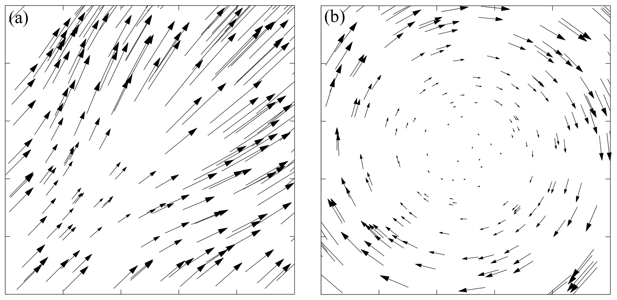
Figure 11Forcing fields of (a) wind velocity and (b) ocean velocity used in a square domain test case.
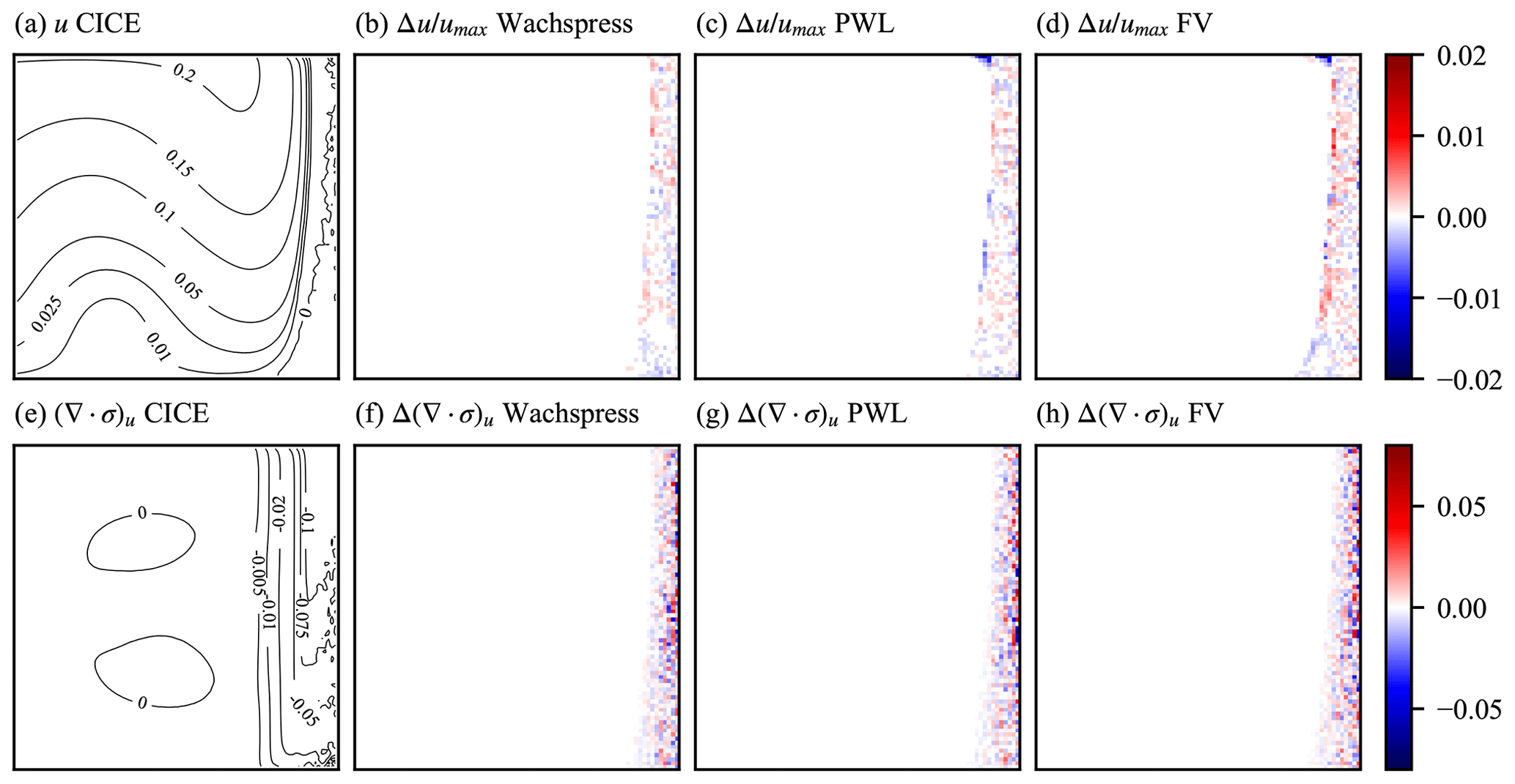
Figure 12(a) The u velocity component of CICE for the square domain test case using a quadrilateral mesh. (b, c, d) Difference () between the u component of MPAS-Seaice and CICE in the square domain test case for the MPAS-Seaice Wachspress variational, PWL variational, and finite-volume (FV) schemes, respectively, and using a quadrilateral mesh. (e)–(h) As (a)–(d) but for the u component of the divergence of internal ice stress.
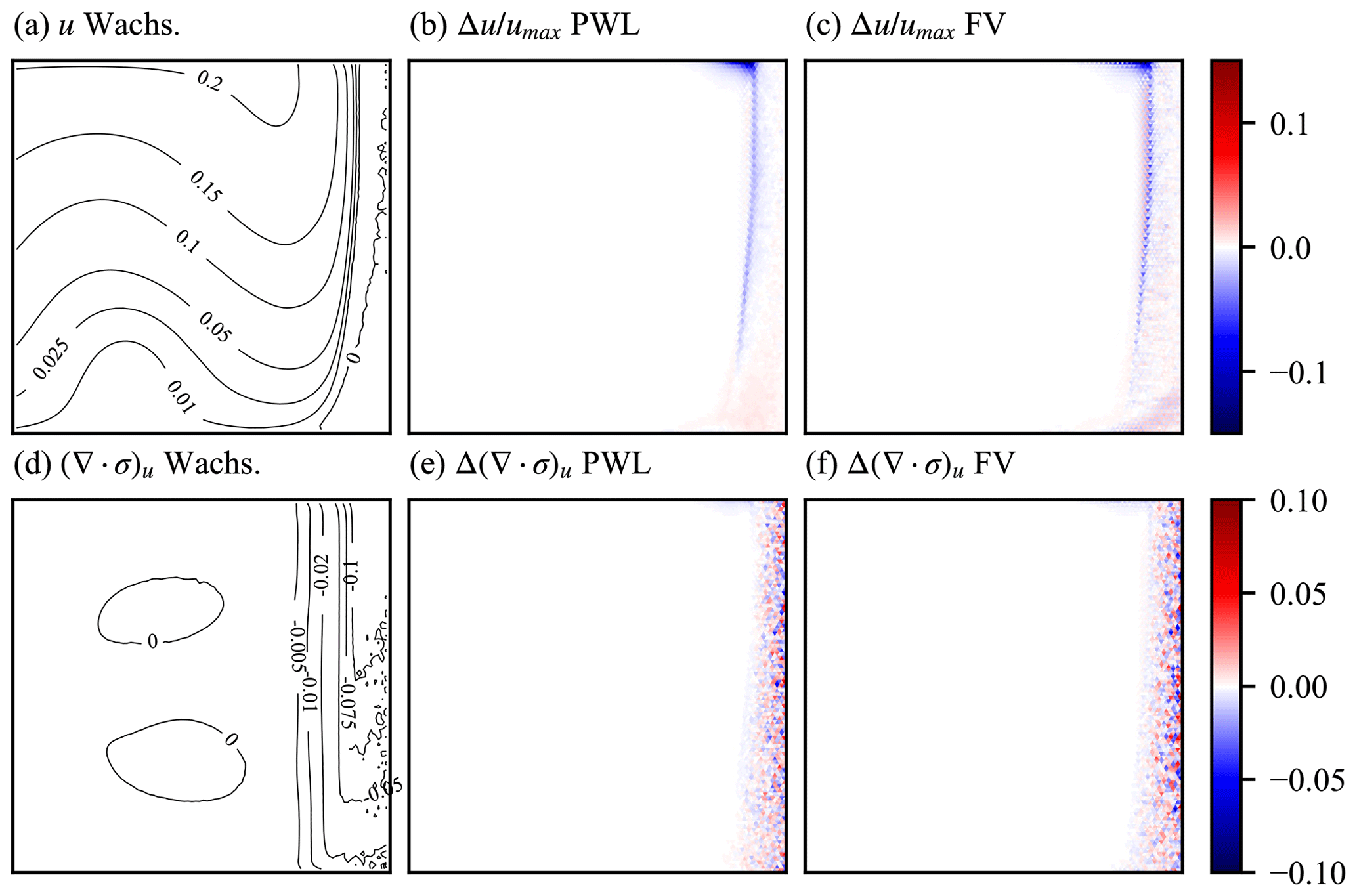
Figure 13(a) The u velocity component of MPAS-Seaice with the Wachspress variational scheme for the square domain test case using hexagonal elements. (b, c) Difference () between the u component of MPAS-Seaice using the Wachspress variational scheme and MPAS-Seaice using the PWL variational and finite-volume (FV) schemes, respectively, in the square domain test case using hexagonal cells. (d)–(f) As (a)–(c) but for the u component of the divergence of internal ice stress.
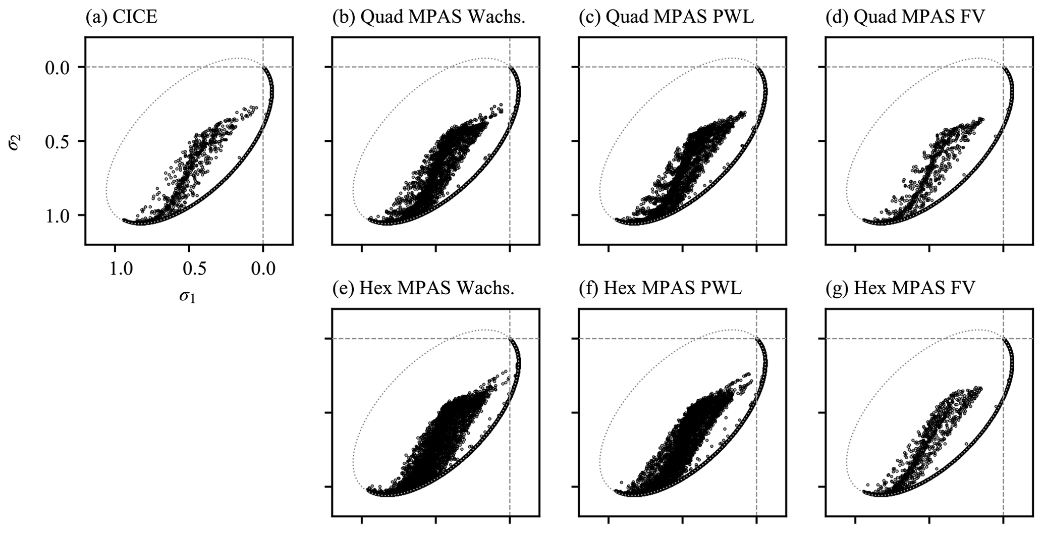
Figure 14Principal stress components for the square domain test case and (dotted) the EVP yield curve. (a) CICE. (b–d) MPAS-Seaice on a quadrilateral mesh and using the Wachspress variational, PWL variational, and finite-volume (FV) schemes, respectively. (e–g) MPAS-Seaice on a hexagonal mesh and using the Wachspress variational, PWL variational, and finite-volume (FV) schemes, respectively.
3.2 Transport
To verify that the incremental remapping transport scheme works as expected, we ran two test cases on a global spherical grid, following Lipscomb and Ringler (2005). In each case there is a steady eastward velocity field given by , where , and R is the Earth's radius. We first advect a circular region of ice that has initial concentration given by a cosine bell within a distance of a central point on the Equator, and a=0 elsewhere. The initial ice thickness is h=1. We compare results from the IR scheme to a simple first-order upwind scheme to demonstrate the improvements in numerical diffusion gained by increasing the order of transport scheme. For both the IR scheme and the first-order upwind scheme, the model was run at several grid resolutions for 12 d, at which time a perfect advection scheme would give a solution equal to the initial condition. For a grid resolution of 120 km, Fig. 15a shows equatorial cross sections of a for the initial condition, the upwind solution, and the IR solution. Figure 16a–c show the spatial distribution of ice concentration before and after the experiment for the same resolution. As expected, the upwind solution is very diffuse, while the IR scheme does a much better job of preserving the initial shape.
Next, we advect a slotted cylinder with initial concentration a=1, initial thickness h=1, and radius , also centered on the Equator. We set for and also in a slot of width and length , with the long axis perpendicular to the flow. The model was run for 12 d at several resolutions. Figure 15b shows the initial condition and the upwind and IR solutions along the Equator at a resolution of 120 km, while Fig. 16d–f show the spatial distribution of the ice concentration before and after the experiment for the same resolution. Again, the upwind scheme is very diffusive; all traces of the slot vanish. The IR scheme does well at maintaining the initial plateaus and a distinct slot, although diffusion into the slot raises the minimum concentration from 0 to ∼ 0.2. Early in the IR simulation there is truncation at the leading and trailing edges of the cylinder, where the gradient is limited, but advection continues thereafter with little change in shape. The maximum concentration is just above 1 because the discretized velocity field is slightly convergent, and diffusion is small. On a plane (not shown) with steady , the discretized velocity field is non-convergent, and a remains bounded by [0,1]. Ice thickness, having been initialized to h=1 everywhere, remains h=1 everywhere (within roundoff), showing that both schemes preserve tracer monotonicity as expected.
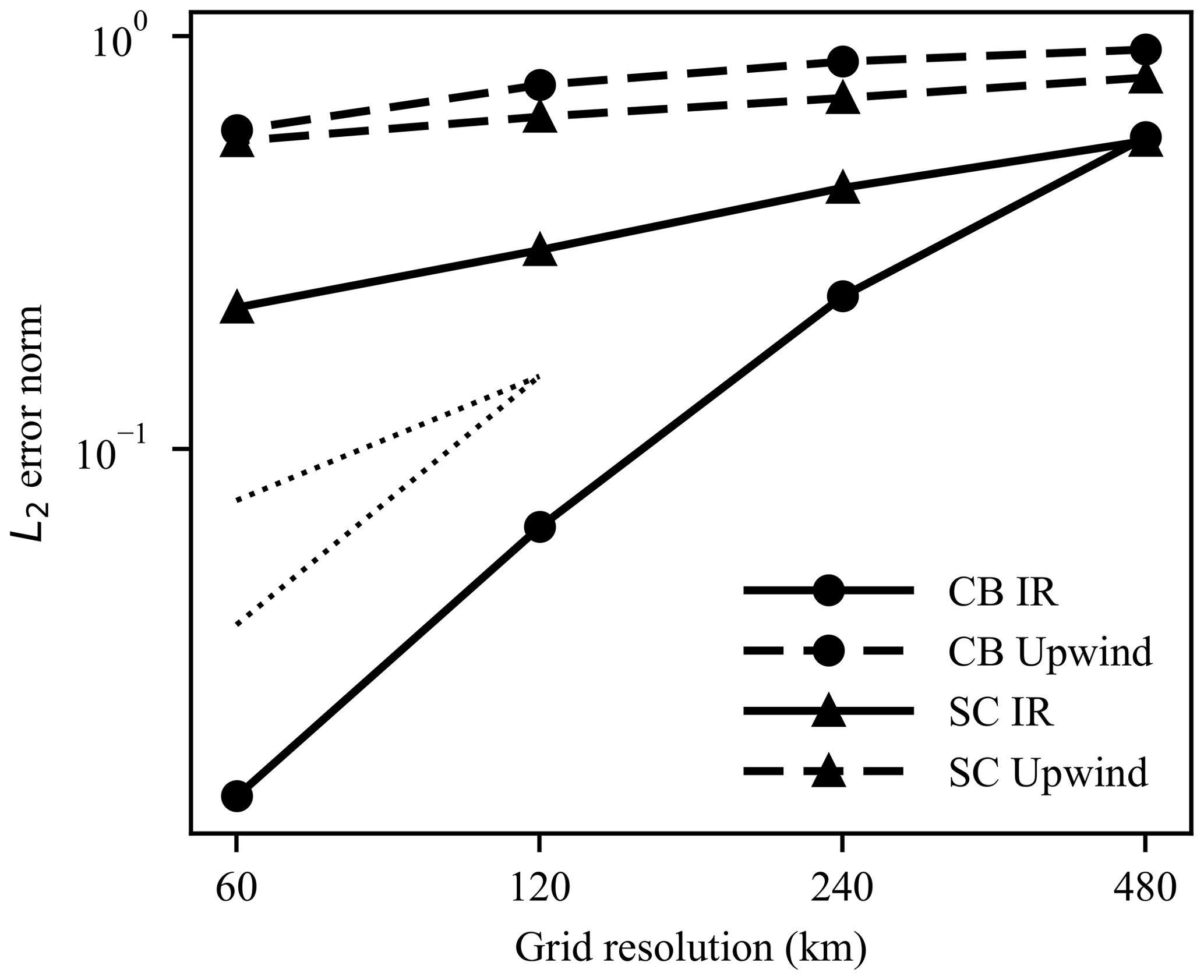
Figure 17 shows the L2 error norm of the 12 d solution for four grid resolutions ranging from 60 to 480 km (where resolution is taken as the mean distance between neighboring cell centers). Figure 17 shows that the IR solution converges with close-to-second-order accuracy (indicated by the dotted diagonal line) for the cosine bell and converges slightly below first-order accuracy for the slotted cylinder. This slow convergence for the slotted cylinder is the result of the ice concentration discontinuity at the cylinder edge, which becomes sharper as the distance between neighboring grid cells decreases when resolution increases. The upwind scheme converges more slowly than the IR scheme, with larger errors at all resolutions. Some along-motion asymmetry is visible in the IR solutions. This is also visible in IR solutions in Lipscomb and Ringler (2005) and is expected since IR is an upstream-based method.
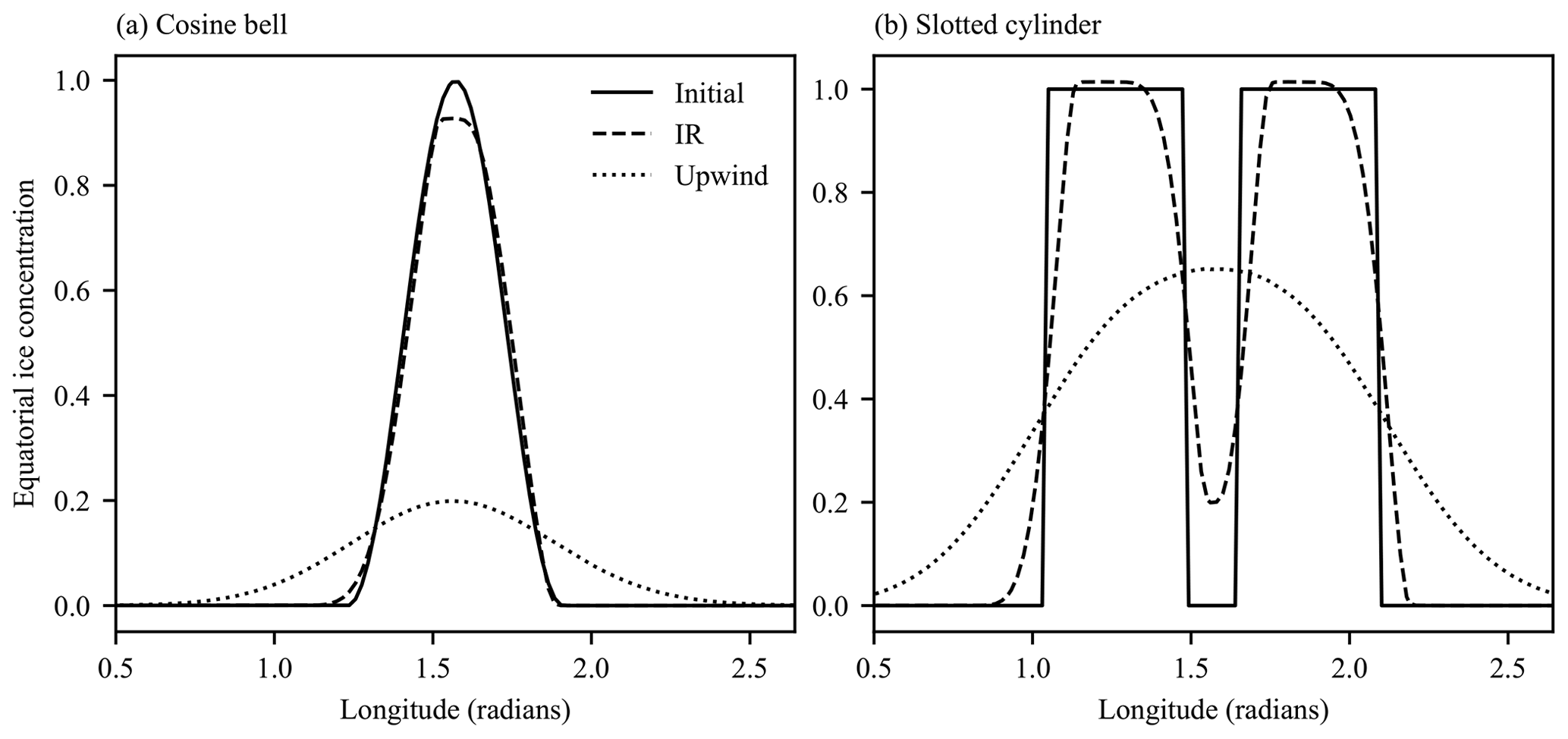
Figure 15Comparison of incremental remapping to a first-order upwind scheme for advection around the sphere. Panel (a) shows a cross section of a circular region of sea ice whose center lies on the Equator, with radius (where R is the Earth's radius) and initial sea-ice concentration given by a cosine bell. Panel (b) shows a cross section of a slotted cylinder whose center lies on the Equator, with radius . The grid resolution is 120 km. The exact solution (which corresponds to the initial condition) is shown by a solid line, IR by long dashes, and upwind by short dashes.

Figure 16Initial (a, d) and final (b, c, e, f) ice concentration contours at 120 km resolution for the cosine bell (a–c) and slotted cylinder (d–f) advection test cases. Results for the upwind advection scheme are shown in (b) and (e), while results from the incremental remapping scheme are shown in (c) and (f). Contours are at levels 0.05, 0.1, 0.3, 0.5, 0.7, 0.9, and 0.95 unless otherwise shown. The direction of transport is to the right.
3.3 Column physics
To validate the column physics in MPAS-Seaice we make use of the fact that CICE and MPAS-Seaice share identical code. CICE and MPAS-Seaice were run with identical forcing and with dynamics disabled. Results from the two models were bit-for-bit identical, indicating a correct implementation of the column physics in MPAS-Seaice.
3.4 Global simulations
To validate the full MPAS-Seaice model in a global setting we perform standalone global simulations and compare simulation results to observational datasets and to the results of simulations conducted with the CICE model (Hunke et al., 2015; release version 5.1.2). We choose version 5.1.2 of CICE to compare against to keep the comparison as clean as possible since this is the CICE version where the CICE and MPAS-Seaice column physics codes diverged. To aid the comparison to CICE we run both models with a 1∘ displaced pole quadrilateral mesh. We perform the simulation for 50 years from 1958 to 2007. Settings for the column physics are the standard ones for CICE (Hunke et al., 2015). For atmospheric and oceanic forcing we repeat the methods used by Hunke et al. (2013) and Hunke and Holland (2007). Air temperature, air specific humidity, and air velocity at 10 m height and 6-hourly frequency are taken from the Coordinated Ocean-ice Reference Experiments (CORE) Corrected Inter-Annual Forcing Version 2.0 (Large and Yeager, 2009; Griffies et al., 2009). Monthly climatologies of precipitation (Griffies et al., 2009) and cloudiness (Röske, 2001) are also used. Downwelling shortwave radiation is calculated from the monthly climatology of cloudiness using the Arctic Ocean Model Intercomparison Project (AOMIP) shortwave forcing formula (Hunke et al., 2015). Downwelling longwave radiation is calculated according to Rosati and Miyakoda (1988). Oceanic inputs, consisting of sea surface salinity, initial sea surface temperature, currents, sea-surface slope, and deep ocean heat flux, come from monthly mean output of 20 years of a Community Climate System Model (CCSM) climate run (b30.009; Collins et al., 2006). The sea surface temperature is determined by a thermodynamic ocean mixed layer parameterization as used in Hunke et al. (2013). All input forcing fields are interpolated linearly in time, although the MPAS forcing functionality can be easily extended to allow interpolation in time with arbitrary order. To get good agreement between CICE and MPAS-Seaice it was necessary to fix several implementation errors in the CICE 5.1.2 forcing scheme. First, CICE 5.1.2 incorrectly repeats the rotation from geographical to coordinate directions for ocean current climatology data. Second, the ocean current forcing routine, rather than reading the surface layer ocean current data for all 12 months of the climatology, instead reads in the first 12 vertical layers for January. These issues have been fixed in CICE 6+.
Figure 18a–f compare total sea-ice extent between the MPAS-Seaice and CICE models and observational values for the years 1988 to 2007 inclusive. The observational sea-ice extent values for the Northern Hemisphere (Cavalieri and Parkinson, 2012; Parkinson et al., 1999) and Southern Hemisphere (Parkinson and Cavalieri, 2012; Zwally et al., 2002) show excellent agreement with both models, with the seasonal cycle of sea-ice extent well represented in both hemispheres. The largest discrepancy occurs in the Southern Hemisphere, where austral summertime sea-ice extent is too low in both models.

Figure 18Sea-ice extent (area with ice concentration greater than 15 %) by year for the Northern Hemisphere (a–c) and Southern Hemisphere (d–f), for MPAS-Seaice (a, d), CICE (b, e), and SSMI satellite observations (c, f). Northern Hemisphere total sea-ice volume by year for (g) MPAS-Seaice, (h) CICE, and (i) PIOMAS.
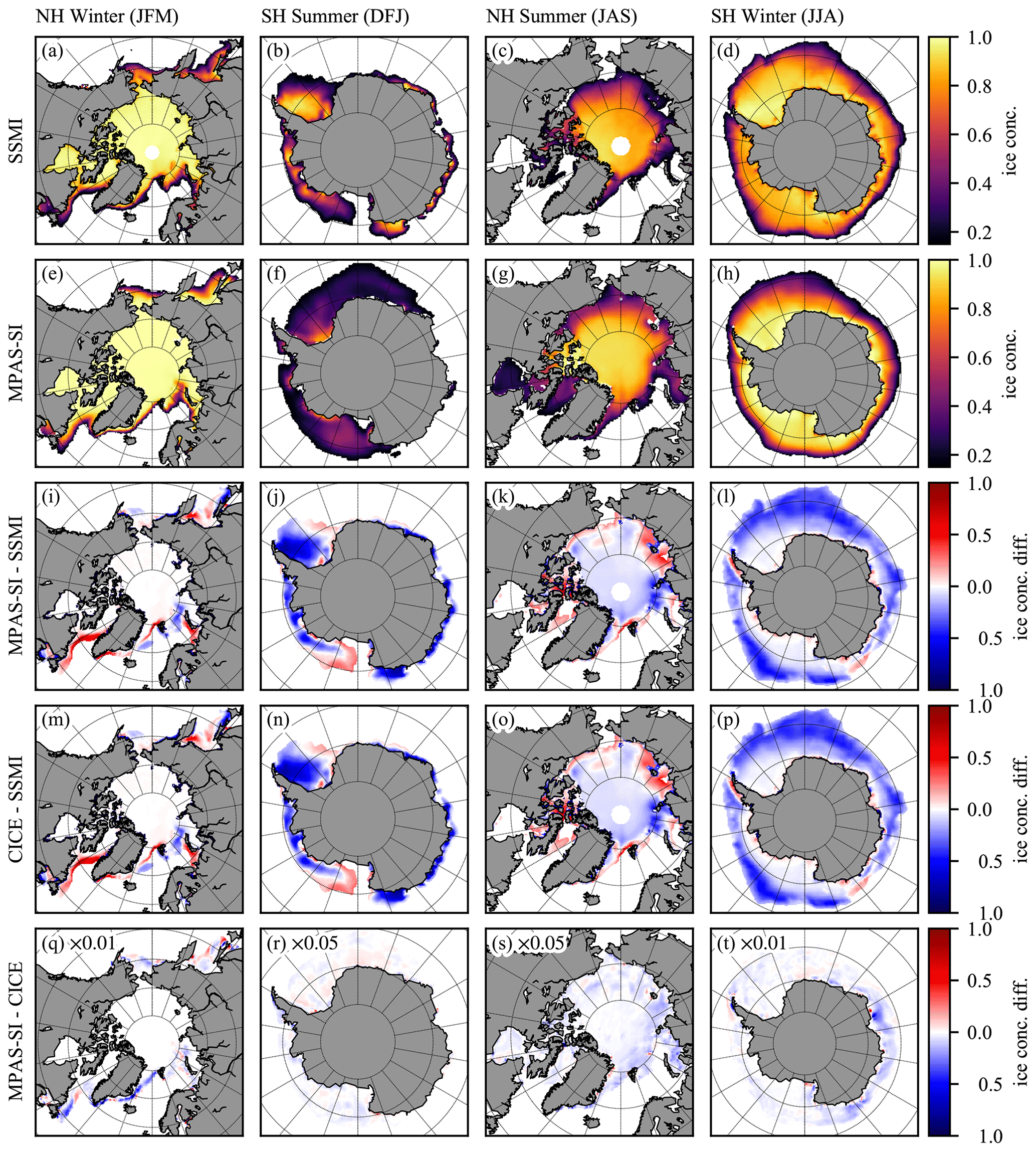
Figure 19Spatial climatological maps for 1988 to 2007 of sea-ice concentration from (a–d) SSMI satellite observations processed with the NASATeam algorithm and (e–h) MPAS-Seaice. Differences between (i–l) MPAS-Seaice and (m–p) CICE ice concentration and SSMI observations. (q–t) Differences between MPAS-Seaice and CICE ice concentration. (a, e, i, m, q) Northern Hemisphere winter: January, February, and March. (b, f, j, n, r) Southern Hemisphere summer: December, January, and February. (c, g, k, o, s) Northern Hemisphere summer: July, August, and September. (d, h, l, p, t) Southern Hemisphere winter: June, July, and August.
Figure 19 shows a similar agreement, comparing sea-ice concentration from Special Sensor Microwave/Imager (SSMI) observations using the NASATeam method (Cavalieri et al., 1996) to model results for summer and winter periods in both hemispheres. Minor differences are present in both models at the Arctic ice edge during winter and in the pack interior in summer. In general the sea-ice extent is well reproduced. In the Southern Hemisphere the sea-ice extent is reasonably reproduced in summer by both models, with more significant differences in the pack interior. As expected from Fig. 18, larger differences are found between the model results and observations in the Southern Hemisphere summer, where ice concentration is particularly underrepresented in the models in the Weddell Sea. In general, agreement is much closer between the two models than between the models and observations. This is expected given the similarity of the models and model forcing. Differences between MPAS-Seaice and CICE are explained by a number of differences in implementation between these models. Firstly, since MPAS-Seaice removes land cells, interpolation between tracer (T) and velocity (U) points (cell centers and vertices in MPAS parlance) does not include zero values for land cells, unlike in CICE. Weights in this interpolation also do not sum exactly to one for CICE since the CICE interpolation scheme mixes T and U cell areas. Secondly, CICE determines the grid angle with respect to geographical coordinates for its T points from averaging over the angle values for surrounding U points. This generates errors in wind and ocean current forcing directions around the North Pole. Finally, for ocean forcing, MPAS-Seaice and CICE have different orders of operation for interpolation in time, space, and rotation from geographical to model coordinate directions, generating small differences in forcing values.
Total sea-ice volume for the Northern Hemisphere is compared between the models and the Pan-Arctic Ice Ocean Modeling and Assimilation System (PIOMAS) assimilated data product (Schweiger et al., 2011) in Fig. 18g–i. Both models and PIOMAS have the expected seasonal cycle with a similar variation between summer and winter and a decrease in total volume over time. Only small differences exist between the two models and the PIOMAS product in terms of absolute ice volume. Figure 20 shows the spatial patterns of sea-ice thickness for the Northern Hemisphere in summer, autumn, and winter compared to observations of sea-ice thickness from ICESat (see Fig. 20 in this paper; Yi and Zwally, 2009). ICESat data are available from set periods from 2003 to 2008 during these seasons, and the model climatological maps are generated for the same periods. ICESat observations exclude sea ice with concentration less than 20 %, so sea-ice thicknesses were excluded from the model results in the comparison where model ice concentration was less than 20 %. Similar spatial patterns of sea ice are found in the results of both models and the ICESat observations, with thicker sea ice along the Canadian archipelago coast and thinner sea ice everywhere at the end of the summer melt season. Both MPAS-Seaice and CICE have excess sea-ice thickness compared to ICESat observations in the Beaufort Sea and western Arctic basin and a deficit of sea-ice thickness in the Eurasian basin.
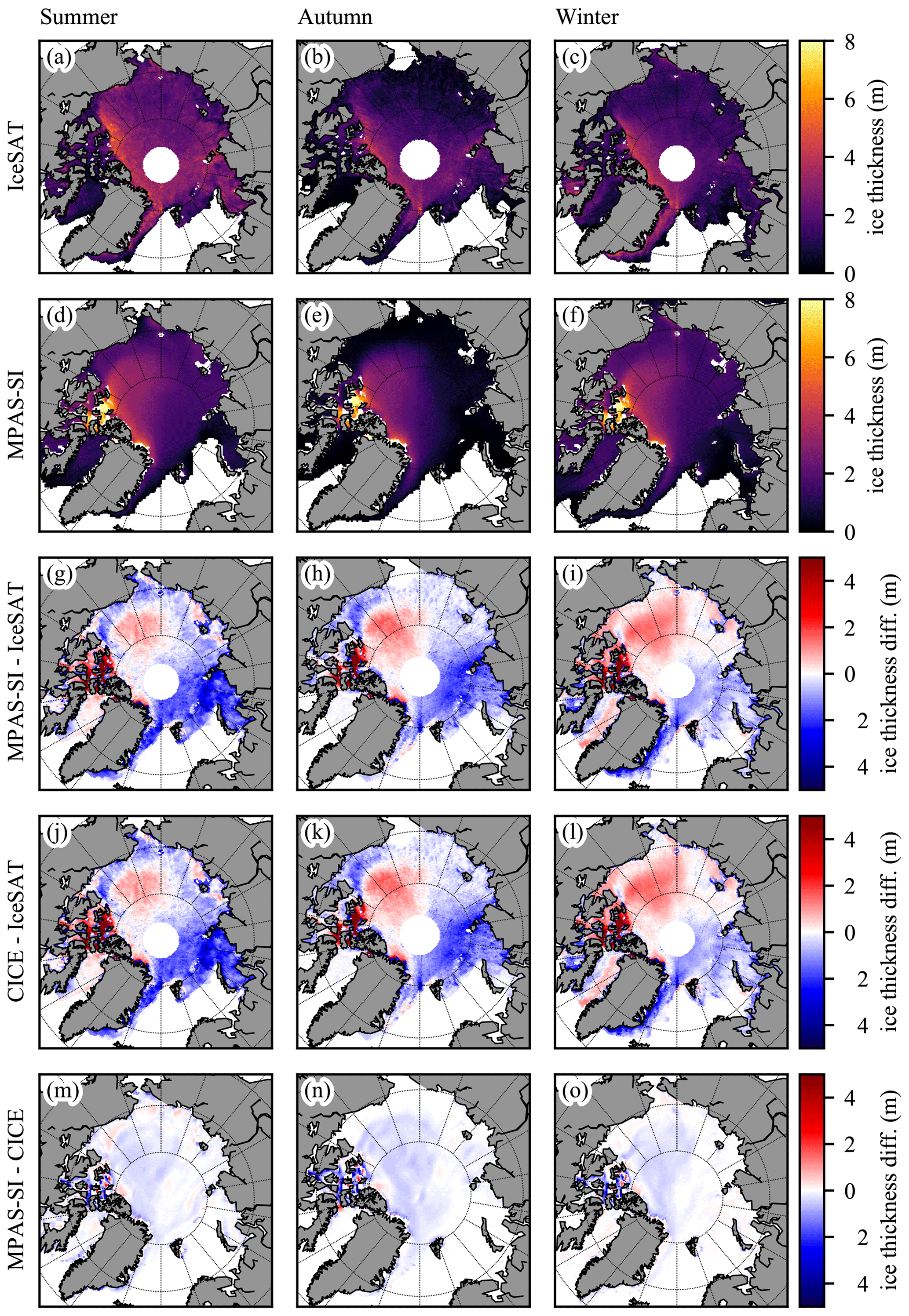
Figure 20Spatial climatological maps of sea-ice thickness from ICESat (a–c) and MPAS-Seaice (d–f). Differences between (g–i) MPAS-Seaice and (j–l) CICE ice thickness and ICESat observations. (m–o) Differences between MPAS-Seaice and CICE ice thickness. (a, d, g, j, m) Northern Hemisphere summer. (b, e, h, k, n) Northern Hemisphere autumn. (c, f, i, l, o) Northern Hemisphere winter.
Finally, we perform simulations with MPAS-Seaice on a quasi-uniform SCVT mesh with 30 km cell separation. The mesh is prepared using the Jigsaw tool (Engwirda, 2017), and the equatorial region is removed for computational efficiency. Figure 21 shows differences in northern- and southern-hemispheric total sea-ice extent and volume between this 30 km SCVT and the 1∘ quadrilateral mesh used above. Results are shown as a percent difference between the meshes with both simulations using the Wachspress variational scheme. Agreement is generally very good, with a difference of only a few percent in extent and volume between the meshes, with the quadrilateral mesh having smaller extent than the SCVT mesh in the Northern Hemisphere and larger extent in the Southern Hemisphere, while volume is lower in both hemispheres for the quadrilateral mesh. The differences also have a strong seasonal variation. We compare several of the other operator methods with the Wachspress variational scheme, all using the quasi-uniform SCVT mesh. While using the alternate area denominator significantly reduced the errors surrounding pentagonal cells in the unit sphere test case in Sect. 3.1.2, it has almost no effect on total ice extent or volume in basin-scale simulations. Compared to the Wachspress variational scheme, the PWL variational and finite-volume schemes have less effect on ice extent and a similar effect on ice volume as compared to the difference between the quasi-uniform SCVT and 1∘ quadrilateral meshes. Differences are also strongly seasonal for these changes in operator, especially for total volume.
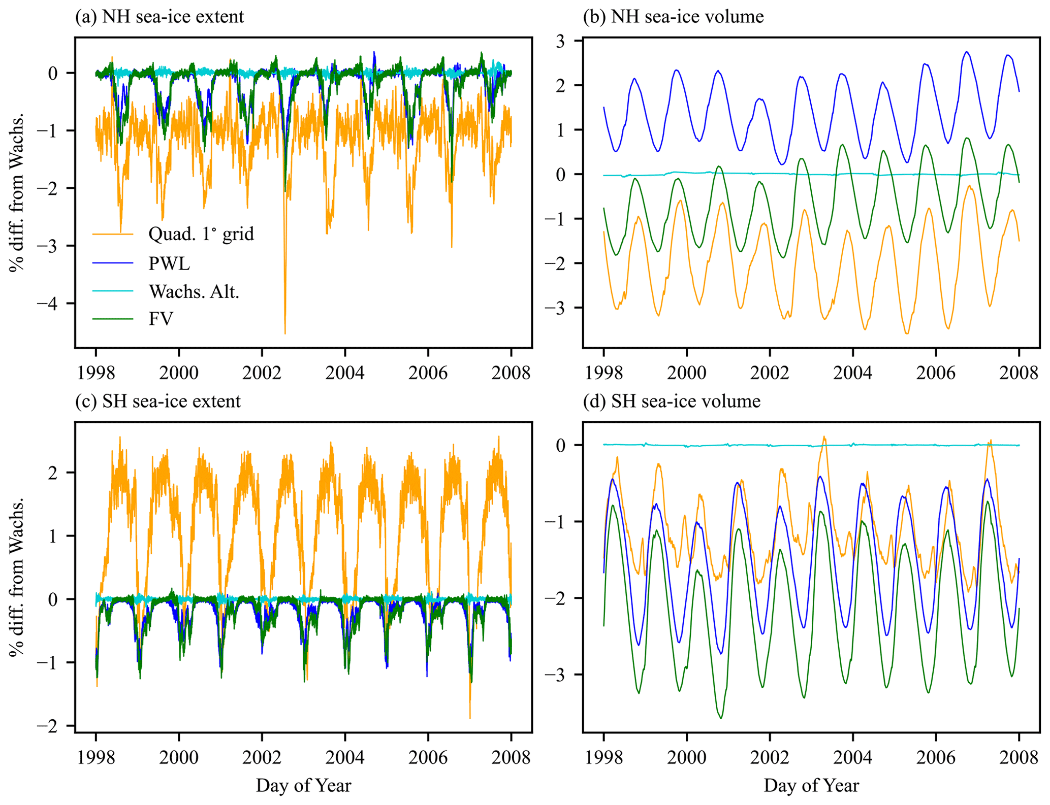
Figure 21Difference (%) in hemispheric sea-ice extent (a, c) and volume (b, d) between global simulations using the Wachspress variational scheme with a quasi-uniform 30 km SCVT mesh and several other simulations. Results are shown for the Northern Hemisphere (a, b) and Southern Hemisphere (b, d).
Through the MPAS framework, MPAS-Seaice incorporates code parallelization through domain decomposition and message passing with the Message Passing Interface (MPI) library. To assess the computational performance of MPAS-Seaice when run on multiple processors, we perform a strong-scaling performance analysis (Fig. 22a). Fixing the grid resolution and run duration, we vary the number of processors and compare the time taken to perform the simulation. We measure model performance in simulated years per day of wall clock time (SYPD). The SYPD metric excludes time spent initializing or finalizing the model simulation but includes time spent reading time-varying forcing data. No output data files are written during these simulations. Simulations were performed as in Sect. 3.4 with a duration of 10 d. Two MPAS meshes are compared. The first is a global quasi-uniform SCVT mesh with cell-to-cell distance of 60 km (QU60km). This mesh has 114 539 cell centers and 234 609 vertices. The MPAS framework allows arbitrary regions of the domain to be removed. We use this capability with MPAS-Seaice by removing equatorial cells where sea ice does not form. This significantly decreases the size of the computational domain and increases computational performance. We use this capability in the second mesh compared, which is the same as the QU60km mesh but with equatorial cells removed, resulting in a mesh with 33 070 cell centers and 69 482 vertices, ∼ 29 % and ∼ 30 % of original cell centers and vertices in the global QU60km mesh. To determine which cells to keep and which to remove, simulations with the full mesh are used to determine a mask of cells where sea ice had ever existed during those simulations. These cells, as well as a buffer region of surrounding cells extending 1000 km further, are kept in the reduced mesh. Removal of equatorial cells produces extra domain boundaries mid-ocean. These are treated as regular land–ocean boundaries, but because of the buffer region mentioned above, during physically reasonable simulations sea ice will not encounter them. Simulations are performed on the Anvil machine at the Laboratory Computing Resource Center at Argonne National Laboratory, which consists of 240 nodes with 36 cores per node.
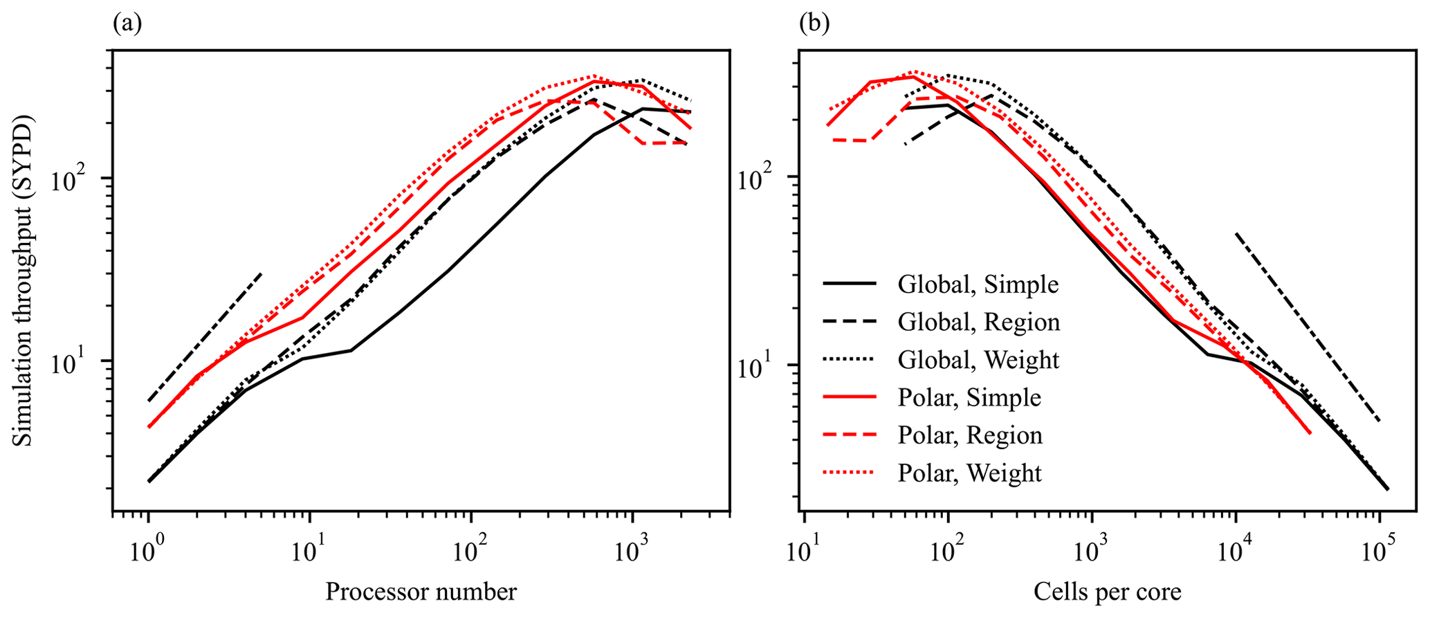
Figure 22Strong-scaling performance characteristics of MPAS-Seaice for a global QU60km mesh (global) and a QU60km mesh with equatorial cells removed (polar). Simulated years per day of wall clock time (SYPD) is plotted against (a) the number of compute cores and (b) cells per core. Perfect strong scaling would be linear for panel (a) and inversely linear for panel (b). Three partitioning methods are employed as described in the main text: simple, region, and weight.
Load balancing is an issue with sea-ice modeling since the presence of sea ice at high latitudes requires more computation for cells located in these regions than in equatorial regions. If the computational domain is partitioned without taking this into account, processors computing high-latitude cells will take longer to compute a time step than processors containing equatorial cells, which will have to wait periodically for high-latitude processors to catch up. This waiting time is wasted and contributes to poor performance. We have implemented three methods to deal with this issue. The first is removing equatorial cells as discussed above. In addition, two improved methods for partitioning the domain across processors have been developed. The standard domain partitioning method for MPAS uses the metis tool (Karypis and Kumar, 1999) to evenly divide the domain amongst processors without taking into account load balancing (labeled “simple” in Fig. 22). The two improved domain partitioning methods aim to give fewer cells and work to processors computing high-latitude regions. The first improved partitioning method (labeled “weight” in Fig. 22) adds a weight to cells in the partition; metis then aims, during the partitioning, to set the sum of weights in each partition equal. Giving high-latitude cells a larger weight than equatorial cells means fewer cells are included in high-latitude partitions, improving load balancing; metis requires this weight to be an integer, which we set to the nearest integer to (1+fn), where f is the fraction of the time the cell in question contains sea ice from a previous simulation. We find that a value of 4 for n maximizes performance. The second improved partitioning method (labeled “region” in Fig. 22) divides the globe into a polar and equatorial region based on the ice presence mask derived from previous simulations. These two regions are individually partitioned, and each processor's domain consists of one partition from the equatorial region and one from the polar region. A processor's computational domain then consists of two discontiguous regions, one polar and one equatorial.
Figure 22a shows slightly sub-linear strong-scaling performance for MPAS-Seaice for both meshes and for the “region” and “weight” partitioning methods below around 400 cores. Above about 400 cores the computational cost of exchanging halo information between processors begins to dominate, and linear scaling is no longer expected. The “simple” partition method also mostly shows near-linear scaling, except at around 10 processors, when load balancing issues begin to affect performance relative to the other partition methods. As expected, removing the equatorial cells reduces this effect. Both the “region” and “weight” partitioning methods improve load balancing by around the same amount. Choice of equatorial mesh removal and partition method can affect performance by up to a factor of around 4. The “region” partition method seems to underperform at high processor number once we reach the limit of strong scaling. This was found to be caused by a deficiency in the generated partitions where, at high processor number, boundaries between partitions would become tortuous. Figure 22b shows the same performance results plotted against the average number of cells per core. Sub-linear scaling is found when the number of cells per core is greater than ∼ 300, with a degradation in performance for simulations with fewer cells per core than this value. A similar result was found for Finite-Element/volumE Sea ice-Ocean Model (FESOM) (Koldunov et al., 2019).
Comparison of computational performance between MPAS-Seaice and CICE is non-trivial. While MPAS-Seaice can be used with quadrilateral meshes, its primary use is expected to be with SCVT meshes consisting primarily of hexagonal cells. The ratio of velocity points to cell centers for these meshes is approximately 2, whereas the quadrilateral grids used by CICE have approximately the same number of velocity points as cell centers. Comparing performance of MPAS-Seaice using SCVT meshes to CICE using quadrilateral meshes then depends on whether the performance is compared based on the number of cell centers or velocity points. To give an approximate idea of the relative performance of MPAS-Seaice and CICE we compare the SYPD achieved on Anvil for 10 d of the simulation described in Sect. 3.4 with both MPAS-Seaice and CICE using a fully global 1∘ quadrilateral grid. Simulation throughput for MPAS-Seaice and CICE is listed in Table 1 as simulated years per day (SYPD) for the whole model and for the velocity solver, transport, and column schemes. For the total model MPAS-Seaice achieved approximately 70 % of the CICE throughput. The better computational performance of CICE is expected since the unstructured mesh in MPAS-Seaice necessitates less efficient memory access patterns. As a percentage of CICE model performance, the MPAS-Seaice velocity solver displayed the poorest throughput and the column physics the most competitive throughput.
Table 1Model throughput (in SYPD) for various code sections for MPAS-Seaice and CICE. Results from 32 processors on Anvil with MPAS-Seaice using the “region” partitioning method and CICE using the “slenderX2” partitioning method.
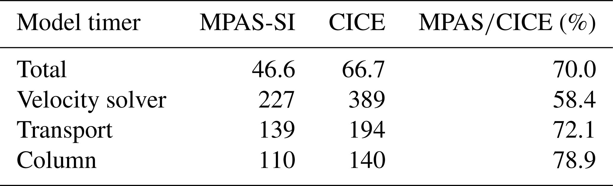
We have described a new sea-ice model, MPAS-Seaice, and successfully validated the velocity solver and transport schemes in idealized test cases, on both planar and spherical grids. These schemes are closely based on those implemented on the quadrilateral grid used in the CICE sea-ice model but adapted for the polygonal cells of MPAS meshes. When using the variational scheme with Wachspress basis functions and a quadrilateral MPAS mesh, the velocity solver of MPAS-Seaice replicates the velocity solver algorithm of CICE, allowing rapid testing and validation.
We developed several other schemes for the strain rate and stress divergence spatial operators to compare with the variational Wachspress scheme. We find that, while the variational scheme, with the alternate area denominator formulation, has excellent error characteristics for the stress divergence operator, the one-sided stencil of the variational strain rate operators results in poor error characteristics. The finite-volume scheme shows the opposite, with good error characteristics for the strain rate operators, but asymmetric integrals around the dual triangles of the SCVT mesh result in larger errors for the finite-volume stress divergence operator. This suggests that the variational scheme could be improved by modifying its strain rate operator to have a two-sided stencil. We investigated several averaging techniques to implement a two-sided stencil for the variational scheme, which resulted in improved error characteristics for the variational strain rate operator. For basin-scale sea-ice simulations, however, these alternate operators had only a small effect on simulation results.
MPAS-Seaice and CICE share the sophisticated suite of column physics and BGC originally developed in CICE, again allowing the rapid development of MPAS-Seaice. Global simulations with realistic forcing have validated MPAS-Seaice against similar simulations with CICE and against observations for sea-ice concentration, extent, and volume. MPAS-Seaice has been coupled into the Energy Exascale Earth System Model (Golaz et al., 2019; Burrows et al., 2020), and the validation experiments described here give confidence in the sea-ice results from E3SM simulations. MPAS-Seaice shows power-law strong-scaling performance with a nearly linear exponent, and the flexibility in mesh partitioning afforded by its use of an unstructured mesh allows efficient load balancing.
Future work will assess the fidelity and performance of MPAS-Seaice on variable-resolution meshes and examine more recent metrics for evaluating sea-ice dynamics, such as new statistical metrics of linear kinematic features (e.g., Hutter and Losch, 2020). Potential challenges with variable-resolution meshes include assessing the resolution invariance of sea-ice rheologies and developing resolution-invariant versions, efficiently using future heterogeneous computing architectures, as well as generating efficient domain partitions of highly variable-resolution meshes.
MPAS-Seaice v1.0.0 is released as part of the Energy Exascale Earth System Model (E3SM) version 2 and is available at https://doi.org/10.11578/E3SM/dc.20210927.1 (E3SM Project, DOE, 2021). Model forcing data are generated by scripts included in the E3SM repository from data available at https://data1.gfdl.noaa.gov/nomads/forms/core/COREv2.html (NOAA, 2021). Other datasets used in this paper are available at https://doi.org/10.5281/zenodo.6230907 (Turner, 2022).
AKT developed and implemented the velocity solver and performed all simulations and analysis. WHL developed and implemented the transport scheme. ECH, AKT, and NJ packaged the thermodynamics into the Icepack library used by MPAS-Seaice. DE provided support for the analysis of the horizontal operators. TDR contributed to the development of the velocity solver. JDW provided software support. DWJ provided support for use of the MPAS framework. AKT prepared the manuscript with contributions from all co-authors.
The contact author has declared that neither they nor their co-authors have any competing interests.
Publisher’s note: Copernicus Publications remains neutral with regard to jurisdictional claims in published maps and institutional affiliations.
This research was supported as part of the Energy Exascale Earth System Model (E3SM) project, funded by the US Department of Energy, Office of Science, Office of Biological and Environmental Research. The National Center for Atmospheric Research is a major facility sponsored by the National Science Foundation under cooperative agreement no. 1852977. This research used a high-performance computing cluster provided by the BER Earth System Modeling program and operated by the Laboratory Computing Resource Center at Argonne National Laboratory. The authors would like to thank Michael Duda of the National Center for Atmospheric Research for his contributions to the MPAS software infrastructure and Sara Calandrini (LANL) for help with mesh generation. Adrian K. Turner would like to thank the Linda Hall Library for access to their collection.
This research has been supported by the Office of Science (grant no. 89233218CNA000001).
This paper was edited by Riccardo Farneti and reviewed by Sergey Danilov and two anonymous referees.
Arakawa, A. and Lamb, V. R.: Computational Design of the Basic Dynamical Processes of the UCLA General Circulation Model, Methods in Computational Physics: Advances in Research and Applications, 17, 173–265, https://doi.org/10.1016/B978-0-12-460817-7.50009-4, 1977. a, b
Bailey, T. S., Adams, M. L., Yang, B., and Zika, M. R.: A piecewise linear finite element discretization of the diffusion equation for arbitrary polyhedral grids, J. Comput. Phys., 227, 3738–3757, https://doi.org/10.1016/j.jcp.2007.11.026, 2008. a
Batchelor, G. K.: An introduction to fluid dynamics, 1st edn., Cambridge University Press, ISBN 978-0-521-66396-0, https://doi.org/10.1017/CBO9780511800955, 1967. a, b, c
Bern, M. and Plassmann, P.: Mesh Generation, in: Handbook of Computational Geometry, 1st edn., edited by: Sack, J. R. and Urrutia, J., chap. 10, pp. 291–332, North-Holland, Amsterdam, ISBN 978-0-444-82537-7, https://doi.org/10.1016/B978-0-444-82537-7.X5000-1, 2000. a
Bitz, C. M. and Lipscomb, W. H.: An energy-conserving thermodynamic model of sea ice, J. Geophys. Res.-Oceans, 104, 15669–15677, https://doi.org/10.1029/1999JC900100, 1999. a
Briegleb, B. P. and Light, B.: A Delta-Eddington multiple scattering parameterization for solar radiation in the sea ice component of the Community Climate System Model, Tech. Rep. NCAR/TN-472+STR, National Center for Atmospheric Research, Boulder, Colorado USA, https://doi.org/10.5065/D6B27S71, 2007. a
Burrows, S. M., Maltrud, M., Yang, X., Zhu, Q., Jeffery, N., Shi, X., Ricciuto, D., Wang, S., Bisht, G., Tang, J., Wolfe, J., Harrop, B. E., Singh, B., Brent, L., Baldwin, S., Zhou, T., Cameron-Smith, P., Keen, N., Collier, N., Xu, M., Hunke, E. C., Elliott, S. M., Turner, A. K., Li, H., Wang, H., Golaz, J.-C., Bond-Lamberty, B., Hoffman, F. M., Riley, W. J., Thornton, P. E., Calvin, K., and Leung, L. R.: The DOE E3SM v1.1 Biogeochemistry Configuration: Description and Simulated Ecosystem-Climate Responses to Historical Changes in Forcing, J. Adv. Model. Earth Sy., 12, e2019MS001766, https://doi.org/10.1029/2019MS001766, 2020. a
Cavalieri, D. J. and Parkinson, C. L.: Arctic sea ice variability and trends, 1979–2010, The Cryosphere, 6, 881–889, https://doi.org/10.5194/tc-6-881-2012, 2012. a
Cavalieri, D. J., Parkinson, C. L., Gloersen, P., and Zwally, H. J.: Sea ice concentrations from Nimbus-7 SMMR and DMSP SSM/I-SSMIS passive microwave data, version 1, Tech. Rep., NASA National Snow and Ice Data Center Distributed Active Archive Center, Boulder, Colorado USA, https://doi.org/10.5067/8GQ8LZQVL0VL, 1996. a
Chen, C., Gao, G., Qi, J., Proshutinsky, A., Beardsley, R. C., Kowalik, Z., Lin, H., and Cowles, G.: A new high-resolution unstructured grid finite volume Arctic Ocean model (AO-FVCOM): An application for tidal studies, J. Geophys. Res.-Oceans, 114, C08017, https://doi.org/10.1029/2008JC004941, 2009. a
Collins, W. D., Bitz, C. M., Blackmon, M. L., Bonan, G. B., Bretherton, C. S., Carton, J. A., Chang, P., Doney, S. C., Hack, J. J., Henderson, T. B., Kiehl, J. T., Large, W. G., McKenna, D. S., Santer, B. D., and Smith, R. D.: The Community Climate System Model Version 3 (CCSM3), J. Climate, 19, 2122–2143, https://doi.org/10.1175/JCLI3761.1, 2006. a
Danabasoglu, G., Lamarque, J.-F., Bacmeister, J., Bailey, D. A., DuVivier, A. K., Edwards, J., Emmons, L. K., Fasullo, J., Garcia, R., Gettelman, A., Hannay, C., Holland, M. M., Large, W. G., Lauritzen, P. H., Lawrence, D. M., Lenaerts, J. T. M., Lindsay, K., Lipscomb, W. H., Mills, M. J., Neale, R., Oleson, K. W., Otto-Bliesner, B., Phillips, A. S., Sacks, W., Tilmes, S., van Kampenhout, L., Vertenstein, M., Bertini, A., Dennis, J., Deser, C., Fischer, C., Fox-Kemper, B., Kay, J. E., Kinnison, D., Kushner, P. J., Larson, V. E., Long, M. C., Mickelson, S., Moore, J. K., Nienhouse, E., Polvani, L., Rasch, P. J., and Strand, W. G.: The Community Earth System Model Version 2 (CESM2), J. Adv. Model. Earth Sy., 12, e2019MS001916, https://doi.org/10.1029/2019MS001916, 2020. a
Danilov, S., Wang, Q., Timmermann, R., Iakovlev, N., Sidorenko, D., Kimmritz, M., Jung, T., and Schröter, J.: Finite-Element Sea Ice Model (FESIM), version 2, Geosci. Model Dev., 8, 1747–1761, https://doi.org/10.5194/gmd-8-1747-2015, 2015. a
Dasgupta, G.: Interpolants within convex polygons: Wachpress' shape functions, J. Aerospac. Eng., 16, 1–8, https://doi.org/10.1061/(ASCE)0893-1321(2003)16:1(1), 2003. a
Dukowicz, J. K. and Baumgardner, J. R.: Incremental remapping as a transport/advection algorithm, J. Comput. Phys., 160, 318–335, https://doi.org/10.1006/jcph.2000.6465, 2000. a, b
Dunavant, D. A.: High degree efficient symmetrical Gaussian quadrature rules for the triangle, Int. J. Numer. Meth. Eng., 21, 1129–1148, https://doi.org/10.1002/nme.1620210612, 1985. a, b, c
E3SM Project, DOE: Energy Exascale Earth System Model v2.0, DOE Code [code], https://doi.org/10.11578/E3SM/dc.20210927.1, 2021. a
Engwirda, D.: JIGSAW-GEO (1.0): locally orthogonal staggered unstructured grid generation for general circulation modelling on the sphere, Geosci. Model Dev., 10, 2117–2140, https://doi.org/10.5194/gmd-10-2117-2017, 2017. a
Flocco, D., Feltham, D. L., and Turner, A. K.: Incorporation of a physically based melt pond scheme into the sea ice component of a climate model, J. Geophys. Res.-Oceans, 115, C08012, https://doi.org/10.1029/2009JC005568, 2010. a
Gao, G., Chen, C., Qi, J., and Beardsley, R. C.: An unstructured-grid, finite-volume sea ice model: Development, validation, and application, J. Geophys. Res.-Oceans, 116, C00D04, https://doi.org/10.1029/2010JC006688, 2011. a
Golaz, J.-C., Caldwell, P. M., Van Roekel, L. P., Petersen, M. R., Tang, Q., Wolfe, J. D., Abeshu, G., Anantharaj, V., Asay-Davis, X. S., Bader, D. C., Baldwin, S. A., Bisht, G., Bogenschutz, P. A., Branstetter, M., Brunke, M. A., Brus, S. R., Burrows, S. M., Cameron-Smith, P. J., Donahue, A. S., Deakin, M., Easter, R. C., Evans, K. J., Feng, Y., Flanner, M., Foucar, J. G., Fyke, J. G., Griffin, B. M., Hannay, C., Harrop, B. E., Hoffman, M. J., Hunke, E. C., Jacob, R. L., Jacobsen, D. W., Jeffery, N., Jones, P. W., Keen, N. D., Klein, S. A., Larson, V. E., Leung, L. R., Li, H.-Y., Lin, W., Lipscomb, W. H., Ma, P.-L., Mahajan, S., Maltrud, M. E., Mametjanov, A., McClean, J. L., McCoy, R. B., Neale, R. B., Price, S. F., Qian, Y., Rasch, P. J., Reeves Eyre, J. E. J., Riley, W. J., Ringler, T. D., Roberts, A. F., Roesler, E. L., Salinger, A. G., Shaheen, Z., Shi, X., Singh, B., Tang, J., Taylor, M. A., Thornton, P. E., Turner, A. K., Veneziani, M., Wan, H., Wang, H., Wang, S., Williams, D. N., Wolfram, P. J., Worley, P. H., Xie, S., Yang, Y., Yoon, J.-H., Zelinka, M. D., Zender, C. S., Zeng, X., Zhang, C., Zhang, K., Zhang, Y., Zheng, X., Zhou, T., and Zhu, Q.: The DOE E3SM Coupled Model Version 1: Overview and Evaluation at Standard Resolution, J. Adv. Model. Earth Sy., 11, 2089–2129, https://doi.org/10.1029/2018MS001603, 2019. a, b
Griffies, S. M., Biastoch, A., Böning, C., Bryan, F., Danabasoglu, G., Chassignet, E. P., England, M. H., Gerdes, R., Haak, H., Hallberg, R. W., Hazeleger, W., Jungclaus, J., Large, W. G., Madec, G., Pirani, A., Samuels, B. L., Scheinert, M., Gupta, A. S., Severijns, C. A., Simmons, H. L., Treguier, A. M., Winton, M., Yeager, S., and Yin, J.: Coordinated Ocean-ice Reference Experiments (COREs), Ocean Model., 26, 1–46, https://doi.org/10.1016/j.ocemod.2008.08.007, 2009. a, b
Hibler, W. D.: A dynamic thermodynamic sea ice model, J. Phys. Oceanogr., 9, 815–846, https://doi.org/10.1175/1520-0485(1979)009<0815:ADTSIM>2.0.CO;2, 1979. a, b
Hoffman, M. J., Perego, M., Price, S. F., Lipscomb, W. H., Zhang, T., Jacobsen, D., Tezaur, I., Salinger, A. G., Tuminaro, R., and Bertagna, L.: MPAS-Albany Land Ice (MALI): a variable-resolution ice sheet model for Earth system modeling using Voronoi grids, Geosci. Model Dev., 11, 3747–3780, https://doi.org/10.5194/gmd-11-3747-2018, 2018. a
Holland, M. M., Bailey, D. A., Briegleb, B. P., Light, B., and Hunke, E.: Improved sea ice shortwave radiation physics in CCSM4: The impact of melt ponds and aerosols on arctic sea ice, J. Climate, 25, 1413–1430, https://doi.org/10.1175/JCLI-D-11-00078.1, 2012. a, b
Hunke, E., Allard, R., Bailey, D., Blain, P., Craig, T., Damsgaard, A., Dupont, F., DuVivier, A., Grumbine, R., Holland, M., Jeffery, N., Lemieux, J.-F., Roberts, A., Turner, M., and Winton, M.: CICE Consortium/Icepack version 1.1.0 (Version Icepack1.1.0), Zenodo [data set], https://doi.org/10.5281/zenodo.1891650, 2018. a
Hunke, E. C.: Viscous-plastic sea ice dynamics with the EVP model: Linearization issues, J. Comput. Phys., 170, 18–38, https://doi.org/10.1006/jcph.2001.6710, 2001. a, b, c
Hunke, E. C. and Dukowicz, J. K.: An elastic-viscous-plastic model for sea ice dynamics, J. Phys. Oceanogr., 27, 1849–1867, https://doi.org/10.1175/1520-0485(1997)027<1849:AEVPMF>2.0.CO;2, 1997. a, b, c, d
Hunke, E. C. and Dukowicz, J. K.: The elastic-viscous-plastic sea ice dynamics model in general orthogonal curvilinear coordinates on a sphere – Incorporation of metric terms, Mon. Weather Rev., 130, 1848–1865, https://doi.org/10.1175/1520-0493(2002)130<1848:TEVPSI>2.0.CO;2, 2002. a, b, c, d, e, f, g
Hunke, E. C. and Holland, M. M.: Global atmospheric forcing data for Arctic ice-ocean modeling, J. Geophys. Res.-Oceans, 112, C04S14, https://doi.org/10.1029/2006JC003640, 2007. a
Hunke, E. C., Hebert, D. A., and Lecomte, O.: Level-ice melt ponds in the Los Alamos sea ice model, CICE, Ocean Model., 71, 26–42, https://doi.org/10.1016/j.ocemod.2012.11.008, 2013. a, b, c
Hunke, E. C., Lipscomb, W. H., Turner, A. K., Jeffery, N., and Elliott, S.: CICE: the Los Alamos sea ice model documentation and software user's manual version 5.1, Tech. Rep., Los Alamos National Laboratory, LA-CC-06-012, https://github.com/CICE-Consortium/CICE-svn-trunk/blob/main/cicedoc/cicedoc.pdf (last access: 4 April 2022), 2015. a, b, c, d, e, f
Hutchings, J. K., Jasak, H., and Laxon, S. W.: A strength implicit correction scheme for the viscous-plastic sea ice model, Ocean Model., 7, 111–133, https://doi.org/10.1016/S1463-5003(03)00040-4, 2004. a
Hutter, N. and Losch, M.: Feature-based comparison of sea ice deformation in lead-permitting sea ice simulations, The Cryosphere, 14, 93–113, https://doi.org/10.5194/tc-14-93-2020, 2020. a
Ingram, W. J., Wilson, C. A., and Mitchell, J. F. B.: Modeling climate change: An assessment of sea ice and surface albedo feedbacks, J. Geophys. Res.-Atmos., 94, 8609–8622, https://doi.org/10.1029/JD094iD06p08609, 1989. a
Jeffery, N. and Hunke, E. C.: Modeling the winter-spring transition of first-year ice in the western Weddell Sea, J. Geophys. Res.-Oceans, 119, 5891–5920, https://doi.org/10.1002/2013JC009634, 2014. a
Jeffery, N., Elliott, S., Hunke, E. C., Lipscomb, W. H., and Turner, A.: Biogeochemistry of CICE: The Los Alamos sea ice model documentation and software user's manual, zbgc_colpkg modifications to version 5.0., Tech. Rep., LA-UR-16-27780, Los Alamos National Laboratory, Los Alamos, NM, USA, https://doi.org/10.2172/1329842, 2016. a
Jeffery, N., Maltrud, M. E., Hunke, E. C., Wang, S., Wolfe, J., Turner, A. K., Burrows, S. M., Shi, X., Lipscomb, W. H., Maslowski, W., and Calvin, K. V.: Investigating controls on sea ice algal production using E3SMv1.1-BGC, Ann. Glaciol., 61, 51–72, https://doi.org/10.1017/aog.2020.7, 2020. a
Karypis, G. and Kumar, V.: A Fast and High Quality Multilevel Scheme for Partitioning Irregular Graphs, SIAM J. Sci. Comput., 20, 359–392, https://doi.org/10.1137/S1064827595287997, 1999. a
Killworth, P. D.: Deep convection in the World Ocean, Rev. Geophys., 21, 1–26, https://doi.org/10.1029/RG021i001p00001, 1983. a
Koldunov, N. V., Aizinger, V., Rakowsky, N., Scholz, P., Sidorenko, D., Danilov, S., and Jung, T.: Scalability and some optimization of the Finite-volumE Sea ice–Ocean Model, Version 2.0 (FESOM2), Geosci. Model Dev., 12, 3991–4012, https://doi.org/10.5194/gmd-12-3991-2019, 2019. a
Large, W. G. and Yeager, S. G.: The global climatology of an interannually varying air–sea flux data set, Clim. Dynam., 33, 341–364, https://doi.org/10.1007/s00382-008-0441-3, 2009. a
Lietaer, O., Fichefet, T., and Legat, V.: The effects of resolving the Canadian Arctic Archipelago in a finite element sea ice model, Ocean Model., 24, 140–152, https://doi.org/10.1016/j.ocemod.2008.06.002, 2008. a
Lipscomb, W. H.: Remapping the thickness distribution in sea ice models, J. Geophys. Res.-Oceans, 106, 13989–14000, https://doi.org/10.1029/2000JC000518, 2001. a
Lipscomb, W. H. and Hunke, E. C.: Modeling sea ice transport using incremental remapping, Mon. Weather Rev., 132, 1341–1354, https://doi.org/10.1175/1520-0493(2004)132<1341:MSITUI>2.0.CO;2, 2004. a, b, c, d
Lipscomb, W. H. and Ringler, T. D.: An incremental remapping transport scheme on a spherical geodesic grid, Mon. Weather Rev., 133, 2335–2350, https://doi.org/10.1175/MWR2983.1, 2005. a, b, c, d, e, f
Lipscomb, W. H., Hunke, E. C., Maslowski, W., and Jakacki, J.: Ridging, strength, and stability in high-resolution sea ice models, J. Geophys. Res.-Oceans, 112, C03S91, https://doi.org/10.1029/2005JC003355, 2007. a
Malvern, L. E.: Introduction to the Mechanics of Continuous Medium, Prentice-Hall, Inc., Englewood Cliffs, ISBN 978-0134876030, 1969. a
Mehlmann, C. and Korn, P.: Sea-ice dynamics on triangular grids, J. Comput. Phys., 428, 110086, https://doi.org/10.1016/j.jcp.2020.110086, 2021. a
Murray, R. J.: Explicit generation of orthogonal grids for ocean models, J. Comput. Phys., 126, 251–273, https://doi.org/10.1006/jcph.1996.0136, 1996. a
NOAA: Version 2 forcing for Coordinated Ocean-ice Reference Experiments (CORE), NOAA [data set], https://data1.gfdl.noaa.gov/nomads/forms/core/COREv2.html, last access: 28 November 2021. a
Parkinson, C. L. and Cavalieri, D. J.: Antarctic sea ice variability and trends, 1979–2010, The Cryosphere, 6, 871–880, https://doi.org/10.5194/tc-6-871-2012, 2012. a
Parkinson, C. L., Cavalieri, D. J., Gloersen, P., Zwally, H. J., and Comiso, J. C.: Arctic sea ice extents, areas, and trends, 1978–1996, J. Geophys. Res.-Oceans, 104, 20837–20856, https://doi.org/10.1029/1999JC900082, 1999. a
Reddy, J. N.: An introduction to the finite element method, 2nd edn., McGraw-Hill, New York, ISBN: 9780070513556, 1993. a
Ringler, T., Thuburn, J., Klemp, J., and Skamarock, W.: A unified approach to energy conservation and potential vorticity dynamics for arbitrarily-structured C-grids, J. Comput. Phys., 229, 3065–3090, https://doi.org/10.1016/j.jcp.2009.12.007, 2010. a, b
Ringler, T., Petersen, M., Higdon, R. L., Jacobsen, D., Jones, P. W., and Maltrud, M.: A multi-resolution approach to global ocean modeling, Ocean Model., 69, 211–232, https://doi.org/10.1016/j.ocemod.2013.04.010, 2013. a, b
Rosati, A. and Miyakoda, K.: A general circulation model for upper ocean simulation, J. Phys. Oceanogr., 18, 1601–1626, https://doi.org/10.1175/1520-0485(1988)018<1601:AGCMFU>2.0.CO;2, 1988. a
Röske, F.: An atlas of surface fluxes based on the ECMWF reanalysis. A climatological data set to force global ocean general circulation models, Tech. Rep., 323, Max-Planck-Inst. Für Meteorol., Hamburg, Germany, http://hdl.handle.net/21.11116/0000-0003-2E85-4 (last access: 4 April 2022), 2001. a
Schweiger, A., Lindsay, R., Zhang, J., Steele, M., Stern, H., and Kwok, R.: Uncertainty in modeled Arctic sea ice volume, J. Geophys. Res.-Oceans, 116, C00D06, https://doi.org/10.1029/2011JC007084, 2011. a
Skamarock, W. C., Klemp, J. B., Duda, M. G., Fowler, L. D., Park, S.-H., and Ringler, T. D.: A multiscale nonhydrostatic atmospheric model using centroidal Voronoi tesselations and C-grid staggering, Mon. Weather Rev., 140, 3090–3105, https://doi.org/10.1175/MWR-D-11-00215.1, 2012. a
Smith, R., Kortas, S., and Meltz, B.: Curvilinear coordinates for global ocean models, Tech. Rep. LA-UR-95-1146, Los Alamos National Laboratory, https://lanl-primo.hosted.exlibrisgroup.com/permalink/f/1hmhmmc/01LANL_ALMA5199299490003761 (last access: 4 April 2022), 1995. a
Turner, A.: MPAS-Seaice v1.0.0 data set, Zenodo [data set], https://doi.org/10.5281/zenodo.6230907, 2022. a
Turner, A. K. and Hunke, E. C.: Impacts of a mushy-layer thermodynamic approach in global sea-ice simulations using the CICE sea-ice model, J. Geophys. Res.-Oceans, 120, 1253–1275, https://doi.org/10.1002/2014JC010358, 2015. a
Turner, A. K., Hunke, E. C., and Bitz, C. M.: Two modes of sea-ice gravity drainage: A parameterization for large-scale modeling, J. Geophys. Res.-Oceans, 118, 2279–2294, https://doi.org/10.1002/jgrc.20171, 2013. a
van Leer, B.: Towards the ultimate conservative difference scheme. V. A second-order sequel to Godunov's method, J. Comput. Phys., 32, 101–136, https://doi.org/10.1016/0021-9991(79)90145-1, 1979. a
Wang, Q., Danilov, S., Sidorenko, D., Timmermann, R., Wekerle, C., Wang, X., Jung, T., and Schröter, J.: The Finite Element Sea Ice-Ocean Model (FESOM) v.1.4: formulation of an ocean general circulation model, Geosci. Model Dev., 7, 663–693, https://doi.org/10.5194/gmd-7-663-2014, 2014. a
Yi, D. and Zwally, H. J.: Arctic sea ice freeboard and thickness, version 1., Tech. Rep., NSIDC: National Snow and Ice Data Center, Boulder, Colorado USA [data set], https://doi.org/10.5067/SXJVJ3A2XIZT, 2009. a
Zwally, H. J., Comiso, J. C., Parkinson, C. L., Cavalieri, D. J., and Gloersen, P.: Variability of Antarctic sea ice 1979–1998, J. Geophys. Res., 107, 3041, https://doi.org/10.1029/2000JC000733, 2002. a