the Creative Commons Attribution 4.0 License.
the Creative Commons Attribution 4.0 License.
 | 06 May 2022
Explicitly modelling microtopography in permafrost landscapes in a land surface model (JULES vn5.4_microtopography)
Eleanor J. Burke
Kjetil Schanke Aas
Inge H. J. Althuizen
Julia Boike
Casper Tai Christiansen
Bernd Etzelmüller
Thomas Friborg
Hanna Lee
Heather Rumbold
Rachael H. Turton
Sebastian Westermann
Sarah E. Chadburn
Microtopography can be a key driver of heterogeneity in the ground thermal and hydrological regime of permafrost landscapes. In turn, this heterogeneity can influence plant communities, methane fluxes, and the initiation of abrupt thaw processes. Here we have implemented a two-tile representation of microtopography in JULES (the Joint UK Land Environment Simulator), where tiles are representative of repeating patterns of elevation difference. Tiles are coupled by lateral flows of water, heat, and redistribution of snow, and a surface water store is added to represent ponding. Simulations are performed of two Siberian polygon sites, (Samoylov and Kytalyk) and two Scandinavian palsa sites (Stordalen and Iškoras).
The model represents the observed differences between greater snow depth in hollows vs. raised areas well. The model also improves soil moisture for hollows vs. the non-tiled configuration (“standard JULES”) though the raised tile remains drier than observed. The modelled differences in snow depths and soil moisture between tiles result in the lower tile soil temperatures being warmer for palsa sites, as in reality. However, when comparing the soil temperatures for July at 20 cm depth, the difference in temperature between tiles, or “temperature splitting”, is smaller than observed (3.2 vs. 5.5 ∘C). Polygons display small (0.2 ∘C) to zero temperature splitting, in agreement with observations. Consequently, methane fluxes are near identical (+0 % to 9 %) to those for standard JULES for polygons, although they can be greater than standard JULES for palsa sites (+10 % to 49 %).
Through a sensitivity analysis we quantify the relative importance of model processes with respect to soil moisture and temperatures, identifying which parameters result in the greatest uncertainty in modelled temperature. Varying the palsa elevation between 0.5 and 3 m has little effect on modelled soil temperatures, showing that using only two tiles can still be a valid representation of sites with a range of palsa elevations. Mire saturation is heavily dependent on landscape-scale drainage. Lateral conductive fluxes, while small, reduce the temperature splitting by ∼ 1 ∘C and correspond to the order of observed lateral degradation rates in peat plateau regions, indicating possible application in an area-based thaw model.
Please read the corrigendum first before continuing.
-
Notice on corrigendum
The requested paper has a corresponding corrigendum published. Please read the corrigendum first before downloading the article.
-
Article
(10011 KB)
- Corrigendum
-
Supplement
(588 KB)
-
The requested paper has a corresponding corrigendum published. Please read the corrigendum first before downloading the article.
- Article
(10011 KB) - Full-text XML
- Corrigendum
-
Supplement
(588 KB) - BibTeX
- EndNote


The permafrost carbon feedback is estimated to be equal to around 2 % to 10 % of our anthropogenic emissions budget under the Paris agreement (Burke et al., 2017b; Comyn-Platt et al., 2018; Gasser et al., 2018; Koven et al., 2015; Hoegh-Guldberg et al., 2018, using the 50th percentile). However, the future fate of permafrost carbon depends on a complex interplay of processes, many of which are not currently included in Earth system models (ESMs). Part of the problem is a question of scale. While the extent of permafrost is vast, processes on the scale of metres compound to create a highly heterogeneous landscape, where different soil moisture and temperatures exist side by side. These processes are often driven by microtopography. Hollows trap snow leading to greater insulation in winter (Gouttevin et al., 2018). Larger snow depths are also found where snow accumulates on the upwind slope of raised areas, which is known to have a controlling effect on the growth of palsas and the presence of permafrost (Seppälä, 1994). Elevation differences also result in hollows being wetter and more conductive in the summer, in addition to having a higher heat capacity. If a pond forms, this can increase the absorption of radiation due to its lower albedo (Lin et al., 2016). Even shallow waterbodies (<1 m) can raise the mean annual sediment temperature by more than 10 ∘C compared to mean annual soil temperatures and have been estimated to increase ground warming under a general climatic warming by a factor of 4 or 5 (Langer et al., 2016). The warmer, wetter areas then experience deeper thaw and increased anaerobic decomposition, producing more methane (Sachs et al., 2010). Localised thawing can be further exacerbated by a positive feedback due to subsidence from melting ground ice in an abrupt thaw event (Walter Anthony et al., 2018). The ease with which methane can be transported out of the soil while avoiding oxidation is in turn controlled by the thickness of the soil oxic layer and the plant communities present (Lai, 2009). Again, these are things which are influenced by small-scale variations, for which microtopography is a key controlling factor (Cooper et al., 2017). While rates of methane emissions from anaerobic decomposition are generally much lower than those of aerobic decomposition and the production of CO2, the high global warming potential (GWP) of methane means the former could be of comparable importance to the permafrost carbon feedback in the short term (Walter Anthony et al., 2018; Turetsky et al., 2020; Schneider von Deimling et al., 2015).
The Joint UK Land Environment Simulator (JULES) (https://jules.jchmr.org/, last access: 14 April 2022) is a community land surface model and is used as the land surface scheme in the UK Earth System Model (UKESM) (Sellar et al., 2019). JULES calculates methane fluxes using the values of the soil temperature and carbon pools for each layer (Clark et al., 2011; Gedney et al., 2004). Since JULES is usually run with a single soil column for each grid cell, these values represent the average values across the grid cell. The flux is then multiplied by a “wetland fraction” calculated by TOPMODEL, based on the position of the water table and the grid cell topographic index (Gedney and Cox, 2003) (Fig. 2). However, the “wetland fraction” of the grid cell is likely to be physically and biogeochemically different to the rest of the grid cell. Specifically, the sub-grid processes already described can result in these wetter areas also being warmer, meaning that the modelled methane flux may be too low. The resolution of these sub-grid processes and the resulting heterogeneity is similarly a key challenge for other global models used for future climate projections and needs to be addressed in order to avoid underestimating the permafrost carbon feedback (Bridgham et al., 2013; Blyth et al., 2021; Aas et al., 2019). This study therefore aims to investigate the hypothesis that explicitly modelling microtopography is essential to accurately modelling the ground moisture, temperature, and hence methane emissions of a permafrost landscape.
Microtopographic features are highly prevalent in the permafrost region, as they can be generated as a result of small-scale processes through the formation or removal of ground ice. While our methods are generally applicable, this study applies our model to two such features, ice wedge polygons and palsas (Fig. 1, J. Boike, © Kartverket, https://www.norgeskart.no/, last access: 10 March 2022). Ice wedge polygons are created where wedge ice forms in cracks created by the thermal contraction of the ground, pushing up the adjacent ground (Lachenbruch, 1962). Polygons are widespread; wedge ice is thought to be ∼ 20 % or more of the uppermost permafrost volume (Liljedahl et al., 2016) and is found in the continuous permafrost zone. Palsas are formed where a localised cold patch of ground causes frost heave, elevating mounds of peat (Seppälä, 1986). These in turn experience shallower snow cover and further heaving. When these mounds are joined to cover a larger area, they are known as peat plateaus. Palsas and peat plateaus are found in the discontinuous and sporadic permafrost zones and are also widespread, albeit not to the extent of polygons (Martin et al., 2019; Kremenetski et al., 2003; Fewster et al., 2020). While it is hard to get an estimate for the total extent of palsas and peat plateaus, permafrost peatlands are estimated to cover 1.7 million square kilometres (Hugelius et al., 2020). The choice of these two landforms affords the opportunity to test our model in climatically distinct regions and using different configurations.
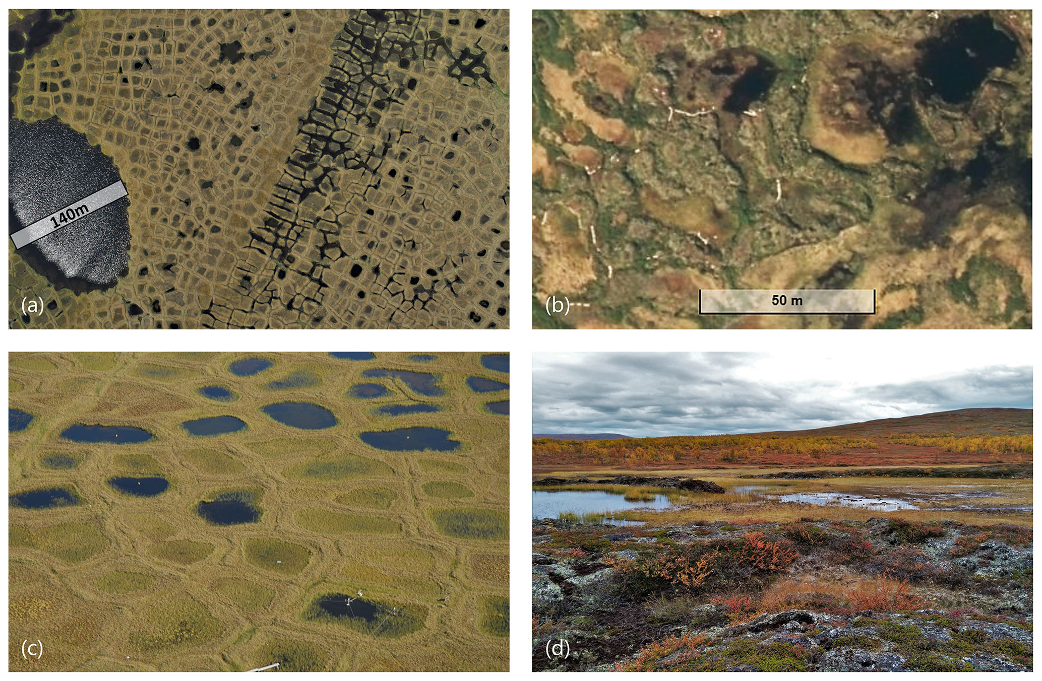
Figure 1Ice wedge polygons at Samoylov (a, c, credit to Julia Boike for the images) and palsas and mire at Iškoras (b, © Kartverket, https://www.norgeskart.no/; d, credit to Noah D. Smith for the image) showing repetitive microtopography and some surface ponding. The observed low-centred polygons at Samoylov were on average 9.1 m in diameter and had rims 0.38 m above the centre. The observed palsa at Iškoras was 0.68 m above the mire. Some polygon rims can reach 1 m in height, while Palsas can reach larger elevations of around to 3 m.
Modelling efforts have been hampered by a lack of long-term high-resolution observations; nevertheless, at a handful of field sites the local variability has been well quantified. Data from these sites have been used to test both high-resolution models of individual features (Jan et al., 2020; Kumar et al., 2016; Grant et al., 2017; Bisht et al., 2018) and low-resolution “tiling” approaches to modelling microtopography and mesotopography (Langer et al., 2016; Aas et al., 2016, 2019; Nitzbon et al., 2019, 2021; Cai et al., 2020; Martin et al., 2021). The reduced computational burden of the latter approach has been pursued as a possible route to representing sub-grid processes in ESMs. These authors have primarily focused on the future evolution of permafrost landscapes, for which they have shown that including microtopography and even mesotopography is essential. When applied on the global scale, a more top-down approach to modelling future permafrost carbon fluxes may be necessary due to the complexity of the feedbacks involved. An example of this method of approach is that taken by Turetsky et al. (2020), who collated observed current rates of abrupt thaw, land type areas, carbon inventories and fluxes and projected these into the future using modelled gradual thaw rates. Similarly, Schneider von Deimling et al. (2015) divide latitudinal bands into different land types with associated carbon pools. Carbon pools and rates for the different land types are set to match observations, and changes in area are scaled by the surface air temperature anomaly from CMIP-5 models under different scenarios. However, these more top-down approaches can result in a loss of flexibility and predictive power, which could result in the omission of potentially important feedbacks. We therefore believe that an explicit tiling approach should be further pursued and developed.
In this paper, we therefore follow the approach of Aas et al. (2019) and Nitzbon et al. (2019) and construct a scheme within JULES where two interacting tiles, offset by an elevation difference, are taken as representative of a repeating microtopographic unit. The relative areas within this repeating unit are then representative of the entire grid cell (Fig. 2). The two-tile approach was chosen as the simplest configuration that still includes an explicit representation of microtopography, as our focus is testing this first step up from the previous implicit microtopography of JULES. For the same reason, dynamically changing areas and elevations, necessary for modelling abrupt thaw processes, as well as a thorough treatment of waterbodies, though important, are not included in the scope of this investigation. Rather, this work aims to strengthen the foundations for applying tiling approaches to microtopography in permafrost landscapes in three main ways. Firstly, we evaluate the efficacy of a two-tile model against microtopographically resolved observations of snow depth, soil temperature, and moisture at four sites. Secondly, we evaluate the importance of explicitly modelling microtopography with regards to its effect on the modelled methane emissions. Thirdly, we quantify the effect of individual model processes, the model's sensitivity to individual model parameters and the resulting uncertainty in the modelled summer soil temperature as a result of uncertainty in those parameters. This sensitivity testing will enable future modellers to assess which model processes should be focused on, which could be simplified, and which parameters most need to be constrained.
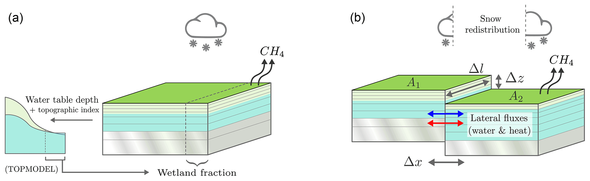
Figure 2The implicit microtopography of standard JULES (a) vs. our explicit approach (b). In standard JULES (a), the grid cell consists of a single soil column representing the average values of soil temperature and carbon. These values are used to calculate a methane flux, which is then multiplied by a wetland fraction (diagnosed by TOPMODEL using the modelled water table depth and the grid cell topographic index). Our explicit approach (b) uses two soil tiles offset by an elevation difference to explicitly simulate areas differentiated by microtopographic processes. Model spatial parameters are shown in grey and are defined for individual sites in Table 2.
2.1 Sites
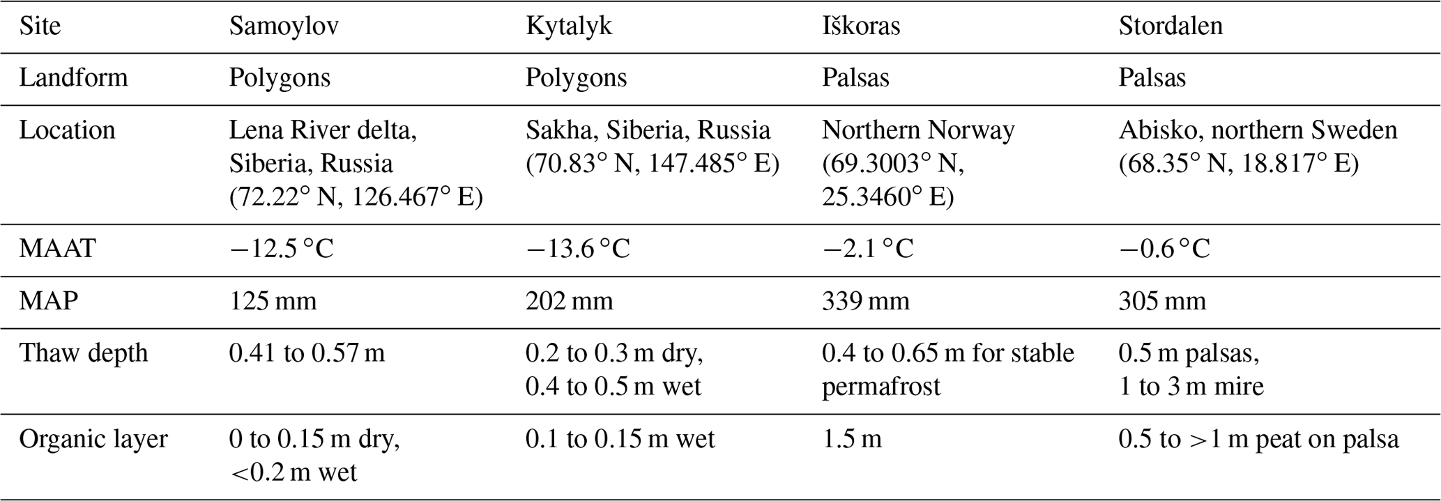
Four sites were used for model validation: two Siberian polygon sites (Samoylov and Kytalyk) and two Scandinavian palsa sites (Stordalen and Iškoras). This choice facilitates comparison, as sites for each type of landform have similar climate, while polygon sites are colder and drier than palsa sites. Table 1 shows a summary of climatic variables for each site, and further site information can be found in Table A1 (Appendix A). Data used from each site can be found in Table A2 (Appendix A). Samoylov, Kytalyk, and Stordalen have already been set up and validated in JULES (Chadburn et al., 2017) and all of these sites have microtopographically resolved data.
Table 1Summary of sites. Further details and sources can be found in Table A1 (Appendix A). MAAT stands for mean annual air temperature, and MAP stands for mean annual precipitation.
Samoylov and Kytalyk are sites with ice-wedge polygons, where observations of soil moisture and temperature used in this paper are for low-centred polygons. Samoylov island is situated in the Lena River delta (Boike et al., 2019). Measurements are from the Holocene terrace on the eastern part of the island. The soil is characterised by alluvial deposits (65 %), with the organic layer underlain by sand and silt with some peat layers. A shallow gradient in the terrace leads to a gradient in hydrological conditions and consequently variation in the degradation of polygons (Nitzbon et al., 2021). Areas of high- and low-centred polygons can be seen, along with a large areal fraction of water surfaces (25 %, Muster et al., 2012). Kytalyk is in a region of Yedoma, with Pleistocene ice deposits occurring nearby in 20 to 30 m tall hills (van der Molen et al., 2007). The measurement site itself is in a depression that was originally a Holocene thermokarst lake. At 2 to 3 m below this is the current river plain, where active thermokarst features are present alongside the river. In addition to ice wedge polygons, Kytalyk has areas of small palsa-like hills (Parmentier et al., 2011). The elevation differences caused by frost heave have led to general difference between dryer elevated areas and lower flooded areas; however, ponding is only seen in small areas (up to 10 %) where ice wedges are actively developing. Precipitation is smaller than that of the palsa sites, but evaporation is limited to the short growing season, meaning the soil can remain wet.
Iškoras and Stordalen are sporadic permafrost sites with palsas surrounded by a lower-elevation, non-permafrost mire. Both have been experiencing lateral degradation of palsas. Stordalen has experienced warming of 2.5 ∘C between 1913 and 2006 (Callaghan et al., 2010) and has lost up to 10 % of the palsa between 1970 and 2000 (Malmer et al., 2005). Stordalen has areas of palsa, ombrotrophic bog that receives runoff from the surrounding palsa, and fen. Drainage out of the palsa follows the frost table via narrow 1 to 2 m long channels (Olefeldt and Roulet, 2012). Unlike the palsa and bog, the fen has no permafrost. In addition to receiving drainage from the bog, the fen receives a large amount of water from a lake just outside the peatland complex and therefore from the 1.7 km2 catchment surrounding it. The Iškoras peat plateau is small, covering an area of ∼ 4 ha, and is surrounded by and interspersed with fen and ponds. Similar drainage channels are observed in palsas, along with typical signs of palsa degradation such as cracking and blocks of peat detaching from palsa edges (Martin et al., 2019).
2.2 JULES
JULES (https://jules.jchmr.org/) is a community land surface model (in Best et al., 2011 and Clark et al., 2011). It is the land surface scheme used in the UK Earth System Model (UKESM) (Sellar et al., 2019) and can also be used as an offline model both globally and at the site level, as is done here. For this study, version 5.4 (http://jules-lsm.github.io/vn5.4/, last access: 2 June 2020) was modified. In JULES a grid cell has a single soil column, on which surface tiles representing different plant functional types and/or non-vegetation tiles such as bare soil, water, and land ice can be used. Each surface tile models its own multi-layer snowpack and canopy water store, and fluxes of heat, water, carbon, and nitrogen are aggregated before exchange with soil layers. For this study, plant competition is modelled by the TRIFFID dynamic vegetation scheme. While the standard configuration of JULES usually has four soil layers with a depth of 3 m, here we use a configuration with 20 soil layers with a total soil depth of 7.8 m as suggested by Chadburn et al. (2015). JULES has been used to model permafrost at the site level, as well as its global extent and the permafrost carbon feedback, including wetland and methane emissions (Chadburn et al., 2015; Burke et al., 2017b; Comyn-Platt et al., 2018; Burke et al., 2017a; Gedney et al., 2019). JULES accounts for the latent heat associated with the freezing and thawing of soil moisture using an apparent heat capacity (Essery et al., 2001), while the unfrozen water content of a layer is calculated from the temperature using a relationship derived from minimising the Gibbs free energy. Frozen and unfrozen water can therefore co-exist, and the liquid water as a fraction of saturation is used to calculate the matric potential of a frozen layer (Cox et al., 1999). The decreased density of water on freezing is, however, not taken into account, and no frost heave effects are modelled.
The version of JULES used here includes two tiles representing either the palsa and mire or the polygon rim and centre. This is done by repeating the same driving data twice within the model. The following developments were included within JULES to improve the representation of microtopography in the northern high latitudes. We have added snow redistribution and lateral water and heat fluxes between the tiles and a surface water store to represent ponding on the lower tile. In addition, we describe the JULES – specific modifications for this model, which are a more conceptually consistent parameterisation of the water table depth diagnostic and a new method of limiting layer numerical over- or under-saturation. Model parameters will be defined as they are encountered but can also be found in Table 2.
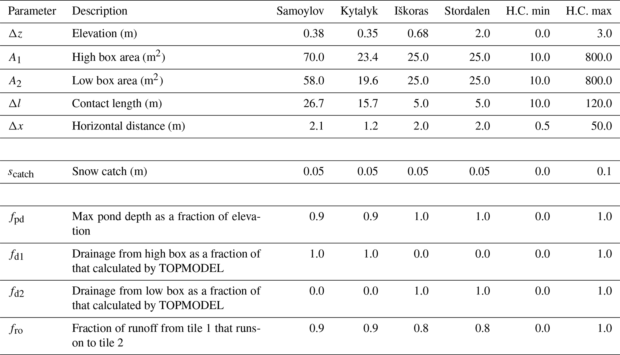
Table 2Estimates of site-specific model parameters. H.C. min and max define the range over which the parameter was varied for the Latin hypercube sampling in the sensitivity study (Sect. 2.5.2).
2.3 Microtopography model additions
2.3.1 Snow redistribution
To model the effects of snow blown by wind on the snow depth of each tile, we use the scheme of Aas et al. (2019) and Nitzbon et al. (2019) where snowfall, S (kg m−2 s−1), is instantaneously partitioned between the two tiles according to the current snow depth on the tiles. We assume that while the current snow depth, d (m), on either tile is less than the snow catch, scatch=0.05 m, the snow is “caught” by vegetation, and thus it cannot be redistributed. In this case, each tile experiences the same snowfall. Snow above this depth is not caught, and thus if the level of snow on the adjacent tile is lower, snowfall will be instantly redistributed to it. A buffer, sbuffer=0.03 m, is applied, such that redistribution does not happen if the elevations differ by less than this amount. This means that once the snow is approximately level, snow is once more able to fall on both tiles. This recreates the observed behaviour of snow filling hollows first (Wainwright et al., 2017; Boike et al., 2018). Finally, as the areas of the tiles may be different, and snowfall in the model is per area, the redistributed snow is subject to an area scaling factor, , where A1 and A2 (m2) are the areas of each tile. The full scheme is described in the equations below.
High to low tile redistribution.
Low to high tile redistribution.
In these schemes, Δz (m) is the elevation difference between tiles and the subscripts “high” and “low” specify the tile with which the variable is associated.
2.3.2 Lateral water fluxes
Lateral flows of water were introduced into JULES using an approach mirroring the existing calculation of vertical fluxes, where fluxes are calculated based on the difference in matric potential between soil layers due to their level of saturation. Existing functions for calculating the layer matric potentials and hydraulic conductivities are used, and the fluxes interfaced into the existing code for the water balance for each layer. Unlike for the vertical fluxes, no implicit correction is used, as fluxes are assumed to be relatively small. Here, fluxes are calculated for horizontal connections, where connections occur between a layer and any other layers horizontally adjacent to it, taking into account the area of overlap of each connection (Fig. 3). However, a “sloped” flow scheme where layers are sequentially connected to their corresponding layer in the neighbouring tile was also considered. Further discussion on the strengths and weaknesses of the two schemes can be found in the Supplement. In JULES, the vertical water flux between layers per land surface area, Wvertical (kg m−2 s−1), is calculated using Darcy's law and is of the following form:
where Kh (kg m−2 s−1) is the hydraulic conductivity, Δzl (m) is the distance between the centres of the layers, and Δψm (m) is the difference in matric potential between layers. When flows are horizontal, the matric potential gradient instead uses the horizontal distance, Δx (m), and as the gravitational potential, ψg (m), remains constant, and the 1 can be dropped. As with the snow scheme, we must go from the intensive form used by JULES of fluxes per land surface area, to the extensive form of kilograms per second through the interface, and back again. The calculated flux is therefore multiplied by area of the interface, ΔvΔl (to go from kg m−2 s−1 to kg s−1), where Δv (m) is the vertical overlap (orange in Fig. 3), and Δl (m) is the contact length. This is then divided by the area of the tile that is being considered, A1 or A2, and thus the change in water content of a layer is still expressed per unit area of that tile. The areal scaling factor for tile n=1 or 2, fq,n is therefore as follows:
where An (m2) denotes the area of tile n. The lateral flow for a connection per surface area of tile n Wh,n (kg m−2 s−1) is therefore calculated as follows:
In JULES, ψm and Kh can be calculated using either the Brooks and Corey (BC) or the Van Genuchten (VG) relations (see Best et al., 2011). Here we use the BC relation for Kh. The VG relation is used for ψm, as it avoids a mismatched ψm when both layers are saturated but is otherwise almost identical to the BC relation for the soil properties of the modelled sites. As in the case for the vertical fluxes, the conductivity is determined using the average liquid water content of the connected layers. This calls into question the use of only two boxes, as for low-centred polygons the soil under the slope between rim and centre has been observed to have a lower saturation than either the polygon rim or centre (Boike et al., 2019), which could lead to the flow being restricted. Not modelling the slope is, however, similar to previous approaches (Aas et al., 2019; Nitzbon et al., 2019) and is the simplest configuration that still models microtopography.
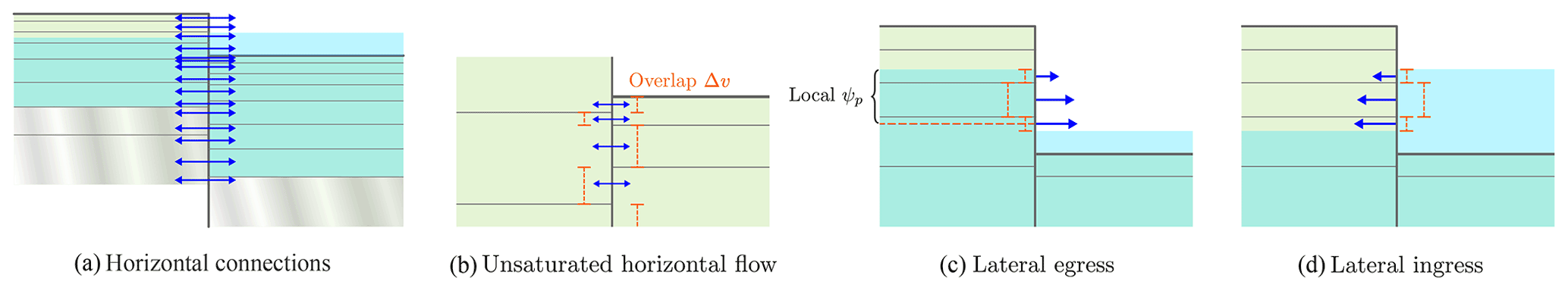
Figure 3The lateral flow scheme. Fluxes are calculated horizontally for connections where layers overlap in the same manner as for the vertical fluxes in JULES (b). Fluxes are only permitted when they are into an unsaturated layer. Where high tile layers are above the low tile soil surface, flow can occur horizontally out of the soil (c) or from the pond to the soil (d).
The horizontal flow scheme raises the question of what to do with the upper layers of the raised tile, which may have no horizontally adjacent layer. If the water table in the elevated tile is above the surface of the lower tile and above the level of the surface of any ponded water (if present), water will be able to laterally egress the soil (Fig. 3c). Similarly, if a pond is present on the low tile and the surface of the pond is above the level of the water table in the high tile, water can flow from the pond laterally into the soil (Fig. 3d). For these flows it is therefore necessary to determine the level of the local water table. For the high tile, for a particular connection, the local pressure head in the high tile ψph (m) is the height of the water table above the midpoint of the vertical overlap (orange in Fig. 3) of the connection being considered. The overlap and midpoint of the connection may be different to the layer thickness and midpoint. This could be due to the layer being partially saturated (the highest overlap in Fig. 3c, and the lowest overlap in Fig. 3d), if only part of the layer is above the pond height (the lowest overlap in Fig. 3c) or if the pond height is between the lower and upper boundary of the unsaturated layer (the highest overlap in Fig. 3d). To calculate the water fluxes for water egress, the difference in potential is Δψ=ψph as there is no matric suction from air. For water ingress, Δψ is the height of the pond above the midpoint of the connection plus the matric suction of the layer the water is entering.
While the local pressure head must be calculated in order for horizontal flows between the soil and the air or the pond and the soil to be modelled, flows are always from a saturated or partially saturated region to an unsaturated one. The model therefore does not implement saturated lateral flows, which are conceptually important for flows between polygons (Wales et al., 2020). This means that advective flows of heat may not be properly represented. However, the model will still be able to act to balance the water table and moisture potentials between tiles, though the rate with which equilibrium is reached may be different. Any discrepancy in rate is, however, expected to be less than the usual timescales over which the water table changes and will therefore not be a problem. The addition of saturated–saturated flows would require solving for the pressure potentials of multiple saturated layers of varying soil properties, which may or may not contain frozen water. This is non-trivial, as the pressure potentials themselves depend on the (now 2D) water fluxes, leading to the requirement for a more complex iterative scheme. On balance, we consider this scheme to be a reasonable simplification for our purposes.
2.3.3 Lateral heat fluxes
Lateral fluxes of heat by conduction and advection use the same connections as the water fluxes. However, of these only the soil-to-soil connections are used, as the pond thermodynamics are not explicitly modelled (it is assumed to be at the surface temperature). The equations for lateral heat flows have the same form as those for the vertical fluxes between layers, as before with the addition of the appropriate areal scaling factors, namely
where Gn (W m−2) and Jn (W m−2) are the conductive and advective heat flows for a lateral connection per surface area of the tile, respectively. As before, n refers to the tile that is being considered. Wn is the lateral water flow from the previous section, ΔT (K) is the temperature difference between laterally adjacent layers and cw (J kg−1 K−1) is the specific heat capacity of water. The average thermal conductivity of the two soil layers λsoil (W m−2 K−1) is calculated using the usual JULES function (Best et al., 2011) and using the mean of the frozen and unfrozen water contents and of the dry soil thermal conductivity for the two layers being considered.
In reality, the heat flux is determined by the continuous derivative . The temperature profile could vary horizontally in a different way to the moisture profile, and indeed would be expected to be asymmetrical across a frozen–unfrozen interface. In the future, the need for a fixed Δx parameter could be eliminated by dynamically determining this profile and including lateral freezing and thawing at the interface. For now, in the model freezing and thawing are effectively distributed evenly throughout the layer undergoing phase change, and we use the same Δx as in the water flux calculation.
2.3.4 Ponding and run-on
In the studied sites, the lower area tends to remain almost saturated year-round (Figs. 5 and 7). However, in standard JULES the surface layers rarely become saturated, as after rainfall events or snowmelt water quickly infiltrates into a space provided by evaporation or, as happens after snowmelt, water is in excess of the maximum infiltration rate and runs off. At both types of site, ponding is common (Boike et al., 2013; Klaminder et al., 2008), both in the centres of polygons and around the edges of palsas. This enables water to gradually infiltrate rather than running off and provides a buffer that enables the soil surface to remain saturated. To model this, a surface water store was added to the low tile. At each time step, a fraction, fro, of runoff from the high tile joins the throughfall of the low tile as run-on, along with the amount of water in the surface water store. Water in excess of the maximum infiltration is then stored in the surface water store. Currently, no thermal effects of the pond are included and so the pond is purely a surface water store. This means that the pond cannot freeze and snow accumulation is unaffected, though in future aspects of FLake (Rooney and Jones, 2010) could be used to introduce these processes in a similar manner to Langer et al. (2016). The only process other than infiltration affected by there being water in the surface water store is that when the pond is present, bare soil evaporation is switched off, and evaporation from the surface water store is equal to the potential evaporation rate calculated by JULES (Best et al., 2011). The ability to pond improves the surface wetness, and if the surface is able to become saturated year-round, the pond can build up to become a persistent waterbody (Fig. 5). When not limited, even in the wettest configuration, pond depths did not rise to more than a couple of metres. However, as this may not physically possible due to the size of the hollow, ponded water in excess of a fraction fpd of the elevation of the high tile is removed as runoff.
2.4 JULES-specific modifications
For this study, we also implemented two modifications to the JULES code that are not of core relevance to modelling microtopography and may not be of relevance to other models that have a different approach to modelling hydrology. Firstly, it was necessary to implement a method of determining the position of the water table within a partially saturated layer in a way that was consistent with the cell-centred method JULES uses to solve the Richard's equation. This was required in order to determine the local water table for a layer. Secondly, the standard methods JULES uses to avoid supersaturation or undersaturation as a result of the water flux calculation numerics (controlled by the switch l_soil_sat_down) can result in the unintended consequence of water being passed out of the soil column. This is particularly a problem for freezing saturated soils. We implemented a new method which avoids this problem (soil_sat_updown) and which also integrates with the scheme for simulating lateral fluxes of water. These modifications are described in the Supplement.
2.5 Setup of simulations
2.5.1 Site parameters
The model is parameterised using observed characteristic dimensions of landscape features present at sites. These parameters are the elevation difference between tiles Δz (m), the areas of each tile A1 and A2 (m2), the contact length between tiles Δl (m) and the horizontal distance between tiles Δx (m) (Fig. 4). For the polygon sites, the raised and lower tiles represent the polygon rim and centre. For the palsa sites, the tiles represent the palsa and mire. The ratios of these parameters determine the model's geometry, and thus the model could also be readily applied to other forms of microtopography. We have approximated ice wedge polygons to have a circular centre surrounded by a ring, , while palsa and mire are represented by squares of equal area with one side in contact, . Δx is the horizontal distance in the calculation of the thermal and hydrological gradient between tiles (Eqs. 5 and 6) and hence a key variable in determining horizontal fluxes of water and heat. Δx is chosen to be representative of the length over which the transition of the thermal and hydrological regimes between the two tiles takes place, as it is this that affects the magnitude of the fluxes. Δx is therefore typically less than the distance between the centres of each tile. The simulations conducted by Abolt et al. (2020) of low-centred polygons in Prudhoe Bay, Alaska, show an approximate distance for this transition that is only slightly longer than the length of the slope between the edge of the flat centre area and the top of the rim (∼ 1 m). We note that the Prudhoe Bay site has a 30 cm organic layer and a relatively sharp transition between rim and centre. These factors, as well as climatic differences, mean that Δx may be different for our sites. We therefore chose values for Δx that are slightly longer than the length of observed transition in topography, noting that these values are similar to those chosen in previous studies (Aas et al., 2016; Nitzbon et al., 2019), but we later test the effect of this assumption in the sensitivity analysis.

Figure 4Geometries indicated by relationships between spatial model parameters for polygons (a) and palsa mires (b).
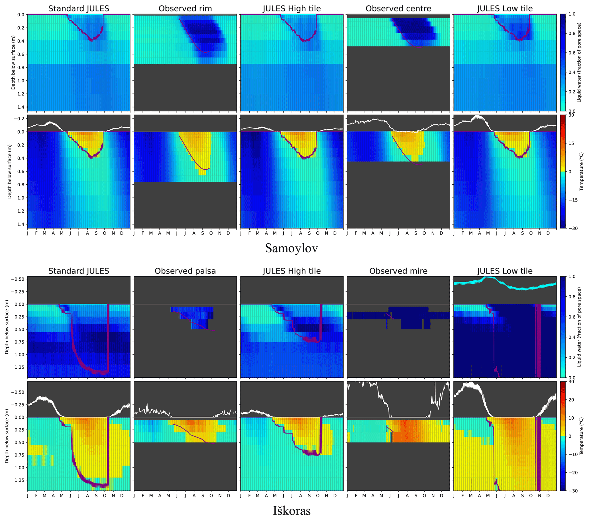
Figure 5Climatologies (2002–2016) providing a comparison of observations with standard and tiled (no qbase) JULES for the polygon site Samoylov and the palsa site Iškoras. The white line above the plots of soil temperature shows snow depth, the cyan line above the plots of simulated soil moisture shows simulated pond depth, and the purple line shows thaw depth. Time series observations are not available for the rim at Samoylov. Figure B6 in Appendix B shows similar overviews for Kytalyk and Stordalen, although these are without observations.
Polygon spatial parameters for Samoylov were found by measuring polygons in the Digital Elevation Map by Boike et al. (2019). Averages were taken over the major and minor axes of each polygon to calculate an average area for the centre. An average of measurements of rim width were then used to calculate the area of an annulus about the centre representing the rim. For Kytalyk, the polygon Lhc11 in Teltewskoi et al. (2019) was used. In both cases, these are low-centred polygons. For the palsa–mire configuration, the geometry of two bordering squares was chosen as a simple configuration representing the edge of a peat plateau, this being an area of interest due to being the site of palsa degradation. In reality, the geometries of peat plateaus are complex, leading to extended perimeters. Indeed, both the perimeter to area ratio and the rate of areal degradation have been observed to increase as palsas become smaller (Borge et al., 2017). The outcome of varying Δl will therefore be of interest for these sites. The chosen geometry for peat plateaus can, however, be a valid representation if a number of assumptions are true. That the border is straight is a good approximation if the border length is small. That the tiles only exchange fluxes on one side relies on gradients of moisture and temperature being small on the other three sides. This ought to be true of the two sides perpendicular to the border due to symmetry and the border being small. Gradients of soil moisture and temperature will also be small at the side furthest from the border if the distance between this side and the border is great enough. Squares of side length 5 m were chosen for both sites as a compromise between these assumptions. The model's sensitivity to this choice was tested later. The elevation used for Iškoras was taken to be the same as the elevation of the palsa where the snow depths were measured (0.68 m) so that results could be validated. This falls towards the lower end of the range for the site observed by Martin et al. (2019), namely 0.1 to 3 m, but is nonetheless an established palsa. Stordalen is a site experiencing degradation, for which Karlgård (2008) gives the characteristic height of 0.5 m, Olefeldt and Roulet (2012) give a range of 0.5 to 2 m, and Klaminder et al. (2008) give a range of 1 to 3 m. Due to the lack of specific microtopographic observations for this site, an elevation difference of 2 m was chosen to provide a contrast to the model setup for Iškoras. The resulting estimates of site-specific model parameters are given in Table 2.
2.5.2 Configurations of JULES simulations
For model code and configuration files, see the code and data availability statement. Each site was spun up in standard JULES (without any microtopographic additions or tiling) for 10 000 years using repeating driving data for the years 1901–1910. Admittedly, this length of spinup turned out to be unnecessary as methane fluxes were ultimately calculated offline using observed carbon profiles. This spun-up state with the additional modification of a saturated soil column was used to initialise the main run (1901–2016) for both standard and tiled JULES. As the same spun-up state was used to investigate multiple configurations which may have different hydrological end states, the soil column was set to be initially saturated for both the spinup and the transient run. This was to avoid the possible development of dry layers during spinup persisting due to being frozen, which could then limit the possible end states (Figs. S6 and S7 in the Supplement). The thermal and hydrological states of the tiles of the transient runs were stable by 1911, and our analysis is limited to the 21st century. Forcing data were prepared as described in Chadburn et al. (2015), where reanalysis data for the grid cell containing each site were adjusted using site observations where available. Water and global change forcing data (WFD) were used for the period 1901–1979 (Weedon et al., 2010, 2011) and WATCH forcing data Era-Interim (WFDEI) were used for the period 1979–2017 (Weedon et al., 2014, 2018). JULES snow parameters are the same as those used in the evaluation of UKESM1 by Sellar et al. (2019), with a fresh snow density of 109 kg m−3. Soil properties for Iškoras were set up using the same method previously used for the other three sites in Chadburn et al. (2017). For Iškoras the profile was assumed to be entirely peat, which is the case for the first 1.55 m in reality (Kjellman et al., 2018) and is a suitable assumption for our analysis. Excess ice is not currently represented in JULES, and thus ice contents need not be initialised.
Parameters specific to the microtopography model for the main tiled runs are given in Tables 2 and 3. For the sensitivity study, three different approaches were used to test the size of the effect of different model processes and the model's sensitivity to its parameters.
-
Additive and subtractive process switching. A series of runs were performed testing the effect of individual processes, where aspects of the model were switched on individually using standard JULES as the base configuration or switched off individually using the full tiled runs as the base configuration.
-
Latin hypercube sampling. A series of 100 runs were performed where model parameters were varied independently using a Latin hypercube sampling, each parameter having an even distribution between the maximum and minimum values given in the columns “H.C. min” and “H.C. max” in Table 2. These runs enable the possible range for an output variable to be gauged, with the caveat that the low ratio of samples to parameters mean that configurations where a number of parameters are at their extreme are unlikely to be sampled.
-
Individually varying parameters. A series of runs where we varied each parameter individually using same maximum and minimum values as for the hypercube sampling, while holding the other parameters at their standard tiled configuration values (as in Table 2). These runs enabled the effects of individual parameters to be disentangled. Using these outputs and estimates of site-specific parameter uncertainties enabled the uncertainty in an output variable due to the uncertainty in a particular parameter to be found.
2.5.3 “Offline” methane analysis
The methane fluxes for each site were estimated “offline” in R using the equations from the methane model in JULES applied to soil carbon and temperature data, similar to part of the analysis in Chadburn et al. (2020). The difference here was that we used a hybrid approach where observed soil carbon profiles were used in combination with modelled soil temperatures (as opposed to using only observations). We took this approach as it removes errors introduced via poor simulation of soil carbon, since the soil carbon was not developed or evaluated in this study. This approach enables the impact of substrate vs. temperature dynamics to be disentangled. For this work we look at methane emissions as calculated by the previous non-microbial version of JULES, as well as by the recently added microbial scheme. The microbial scheme adds a dissolved organic carbon pool, a methanogen pool, and the associated dynamics of methanogenic growth and dormancy. This has been shown to better represent the observed seasonal dynamics (Chadburn et al., 2020).
2.5.4 The qbase configuration (modelling baseflow)
JULES uses TOPMODEL to calculate the baseflow, the saturated flux laterally exiting the grid cell, based on the position of the water table and the distribution of topographic index within the grid cell as described in Gedney and Cox (2003). The calculation is based on the following assumptions: that the water table follows the grid cell topography, that as the water table rises the baseflow increases due to the increasing transmissivity of the saturated zone, and that in the steady state the downslope flow is balanced by the upslope recharge. In JULES this flux is known as qbase and is calculated for and extracted from a layer that contains the water table or that is beneath the water table. Here, we also set qbase to zero for layers that are unsaturated and/or frozen. The total qbase for the grid cell is passed into the river-routing scheme if this is being used but otherwise passes out of the model domain. Each grid cell does not receive any flux from the grid cells surrounding it, and thus this can be viewed as the flux balancing the recharge that the groundwater receives in the grid cell area.
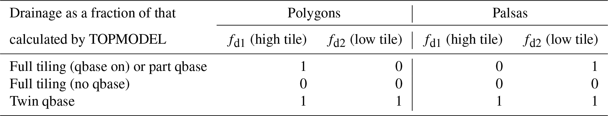
However, in this explicit representation of microtopography, the lateral flows between tiles directly model at least part of this flow. For this reason, we include the parameters fd1 and fd2, which scale the drainage calculated by TOPMODEL applied to the high tile and low tile, respectively. We first considered the configuration where qbase is set to zero for the simulated palsa and for the polygon centre but is on for the other tiles. This configuration is referred to as “qbase on” or “part qbase”, as this is the main configuration where we allow qbase in the model (Table 3). The motivation for this is that there cannot be any drainage from the centres of polygons without going through the rim, and similarly drainage from palsas would usually pass through the surrounding mire. There are two main problems with this approach. Firstly, we are applying a model based on grid-cell-scale assumptions to a subgrid model. This may result in qbase being too great or too small. For instance, rather than being calculated using the grid box average saturation, it is now calculated using the saturation of either the wetter or the drier part of the landscape. This approach could also result in a reduced qbase as it is only being applied to part of the area. Secondly, the lateral drainage calculated by TOPMODEL may not be suitable for some instances of wetland or where a large proportion of the grid cell is wetland. This is partly due to TOPMODEL's limitations in flat landscapes (Koster et al., 2000) but is also due to wetlands being formed in areas where lateral drainage is impeded or even which are fed by groundwater. In JULES, qbase only ever removes water, so the latter is not possible. The repeating nature of landscape units provides motivation for some degree of impedance, as two symmetrical bordering units can have no flow between them. As we expect that qbase may be further impeded, we also consider the configuration, referred to as “no qbase”, where qbase is switched off for both tiles. This is not a general solution and is a departure from standard configurations of JULES. In reality, the lateral landscape-scale drainage will depend on a combination of the mesoscale topography (Nitzbon et al., 2021), the connectivity of the polygon troughs or mire network (Liljedahl et al., 2016; Connon et al., 2014), and the presence of external reservoirs and inter-grid cell flows. These things are beyond the scope of this study and will require further consideration. In addition to these two main configurations for qbase, the response of the model to varying fd1 and fd2 between 0 and 1 was tested in the sensitivity study (as described in Sect. 2.5.2), and a configuration with qbase on for both tiles (“twin qbase”) was included in the model process-switching tests.
Table 3Configurations of the parameters fd1 and fd2, which determine the drainage as a fraction of that calculated by TOPMODEL for each tile.
An overview of the model output can be seen in Fig. 5, which displays climatologies for Samoylov and Iškoras, showing soil moisture and temperature with depth, along with snow depth and modelled pond height, comparing observations with standard and tiled JULES. These results will be expanded in the following sections, which examine the effect of the tiled model on snow, before moving on to soil moisture and temperature and considering which model processes have most effect on these variables. The resulting effect on methane is then considered. Finally, the sensitivity of the model to its parameters is investigated, and sources of uncertainty are identified. Where climatologies are shown, the years shown are for those the model is averaged over, while the years averaged over for observations are for all years available. Date ranges of available soil temperature and moisture measurements are given in Table 4. The forcing data used to drive JULES run from January 1901 to December 2016, and thus overlap with observations for Iškoras was not possible.

3.1 Snow depths
The splitting in snow depths between the tiles as a result of the snow redistribution scheme is shown in Fig. 6. When comparing the average climatologies for Iškoras, where microtopographically resolved time series of snow depth are available, both the snow depths for the top and the base of the palsa are over 20 cm closer to observations for March than the standard JULES simulation. Snow depths for the polygon centre for Samoylov are also closer. The goodness of the model's operation mostly depends on the forcing applied, how well the typical maximum snow height on the elevated areas matches the snow catch, and the tile areas. This is because most of the time the modelled low tile snow depth for these sites does not reach the elevation difference, the point at which snow in the model would build up on both tiles at the same rate. Consequently, the snow depth on the high tile is usually limited by the snow catch parameter (scatch), while the low tile snowfall receives a fixed adjustment of snow for the time that the snow depth is above the snow catch. An alternate “sloped” snow scheme was trialled whereby the fraction of snowfall redistributed varied linearly between all the snowfall being redistributed if the difference in snow elevations equalled the elevation difference between tiles, to no snow redistributed if the snow elevations were equal. The motivation for this scheme was that it might have been more suitable for polygon sites where the slope of the rim gradually becomes more covered in snow as the depth of snow in the centre increases. However, there was little difference between average snow depths for each scheme, so the “sloped” scheme was found to be unnecessary.
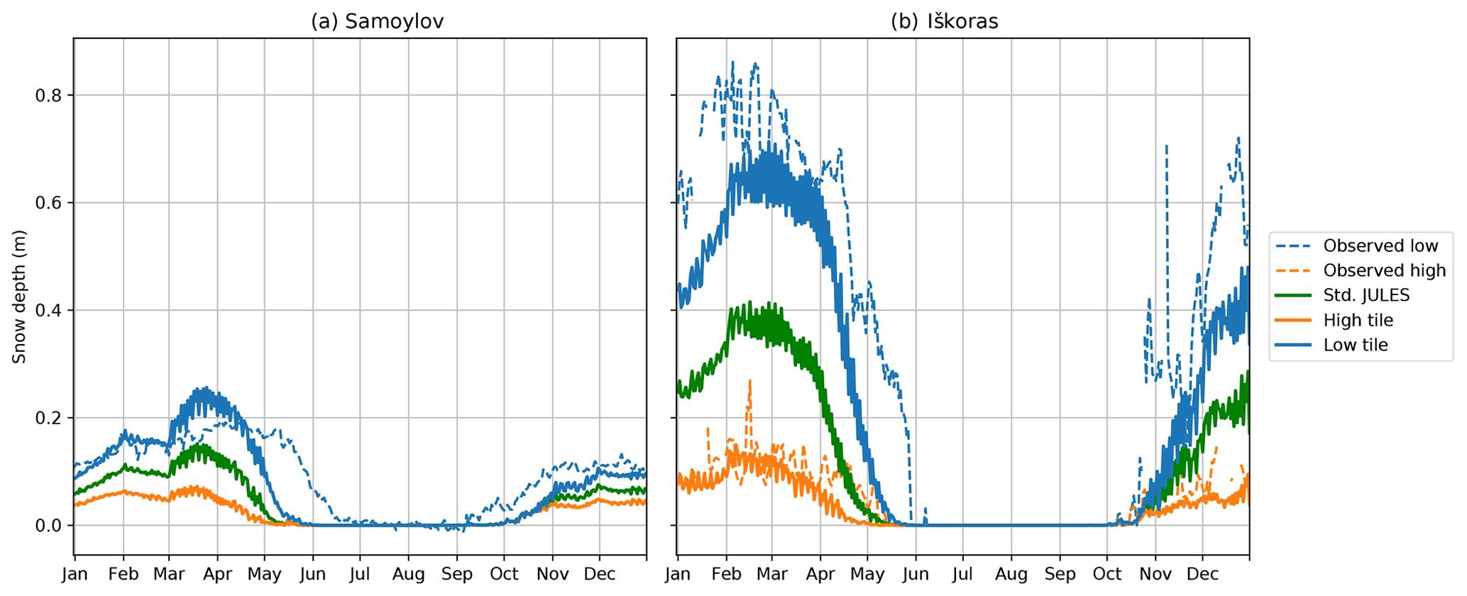
Figure 6Climatology (2002–2016) of simulated vs. observed snow depths for Samoylov (a) and Iškoras (b), showing snow redistribution due to microtopography differentiating snow depths. Observed snow depths for Samoylov have been bias corrected using the signal during the snow-free season.
At Iškoras, while the average climatologies are in relatively good agreement, it is hard to fully gauge the simulation's accuracy as the observed snow depth time series for Iškoras do not overlap the model run period. For Samoylov, the time series do overlap, but only a time series for the centre is available. The full time series for Samoylov is given in Fig. B5, showing the inter-annual variability between the snowfall reanalysis data used to drive the model and the observed snowfall. Figure B5 also shows the median snow depths for the rim and centre measured across multiple polygons by Gouttevin et al. (2018) on their campaign in April 2013; for this date the simulation has the correct depth of snow on the rim, but around 20 to 30 cm too much snow on the centre, when taking into account the observed spatial variability. Some of this discrepancy may be due to the forcing data used. For instance, in the forcing data for Samoylov there is almost no snowfall prior to the start of October, whereas observations indicate snowfall before this, resulting in around 5 cm too little depth of snow for October to January. The scheme also has some obvious omissions. While snow is assumed to be redistributed by wind, wind speed and direction is not input into the snow scheme. Spatial variability due to wind direction and drifting against slopes is therefore not considered. Much of the snow can also be blown a greater distance and accumulates in larger depressions such as lake basins and river gullies, therefore in reality the total balance of snow needs to be considered on a much larger scale. However, a more complete accounting for the spatial variability due to effect of wind speed and direction, topography, and vegetation, as in SnowModel (Liston and Elder, 2006), moves towards needing a detailed gridded representation of topography to run and goes against our aim for a simple representation of subgrid processes. Currently, the snow catch is unaffected by the type and height of vegetation present in the model. Linking the snow catch and vegetation height would be a key next step and would enable snow–vegetation feedbacks to be investigated. Lastly, the properties of the falling snow have no effect on the modelled redistribution, and no consideration is given to wind erosion of the snowpack at a later time after the snow has settled. Zweigel et al. (2021) included the properties of falling snow and the effects of internal snow processes and snow microstructure on snow mobility for a high Arctic site on Svalbard. They found that a thinner layer of lower-density snow built up on their high “ridge” tile than their lower “snowbed” tile, which was then able to be subject to wind erosion at a later time. However, while including these omissions would affect the properties, timing, and spatial variability of the modelled snow redistribution, the snow depths on each tile have still been successfully differentiated with the current model. Collection of additional spatially resolved time series data would enable further validation, investigation of the effect of missing processes and for model parameters to be better constrained.
3.2 Water
Figure 7 shows in black the observed average saturation profiles for July, where sites are grouped according to landscape type due to a lack of detailed observations of hydrology at Kytalyk and Stordalen. For all studied sites, observations show that the lower area is characterised by year-round saturated or almost-saturated conditions, with a water table generally within 10 cm of the surface. Polygon rims are still fairly wet, with the observed water table (shown by box plots) within 20 cm of the surface, while observations from palsas have an unfrozen liquid fractional saturation of around 0.6 at 10–20 cm depth. Observed soil moisture for the palsa at Iškoras at 0.4 m decreases vs. that at 0.2 m due to still being partially frozen in July. Model outputs in Fig. 7 will be discussed in the following sections.
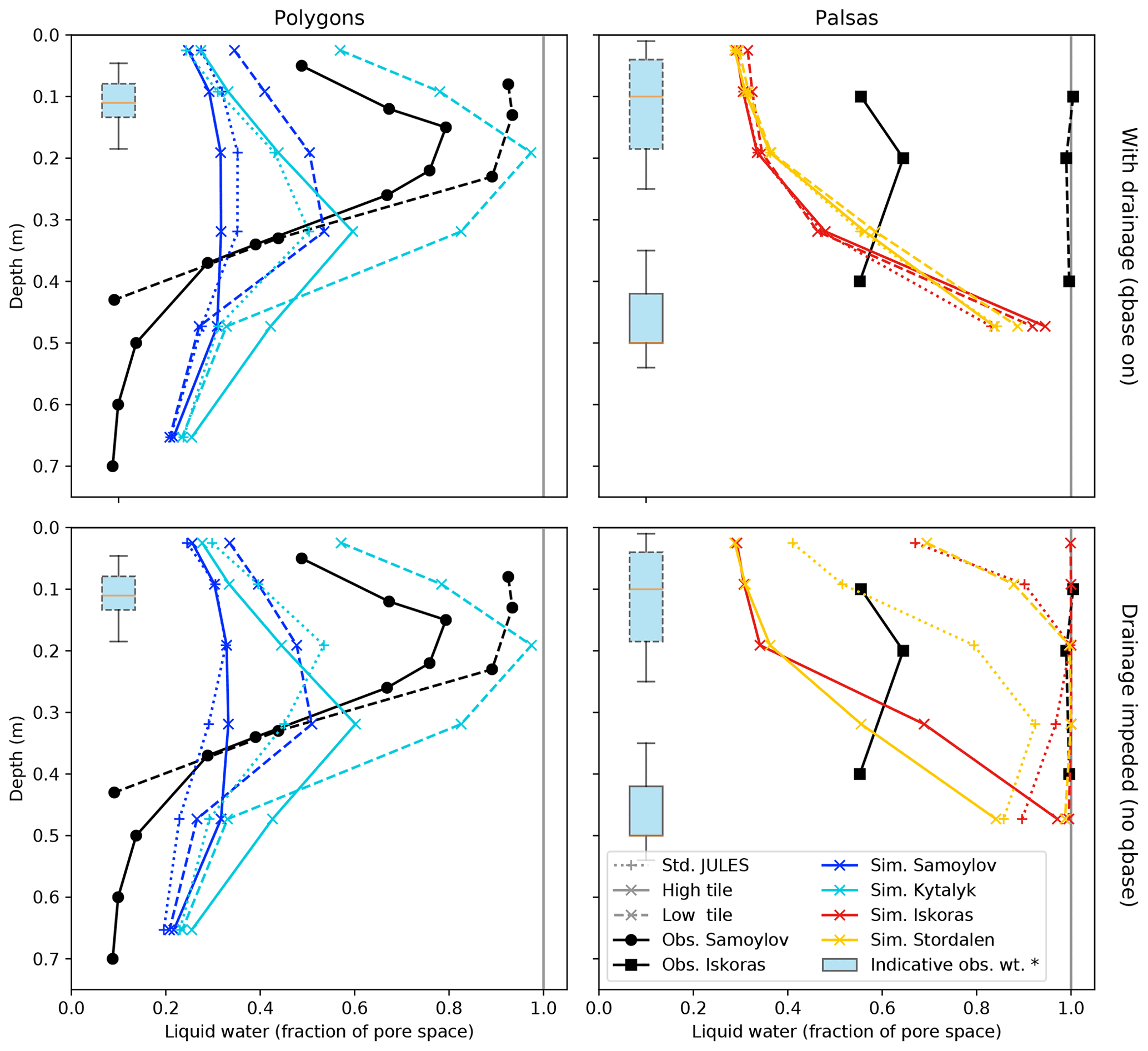
Figure 7Average saturation profiles for July (2000–2016) showing the effect of tiling and also the importance of impeding mire drainage for palsa sites. Line colours show different sites while line styles differentiate high, low, and standard JULES. As points for simulations show the average saturation for the layer whose midpoint is at the depth shown, the simulated water table may be above a partially saturated point. Indicative observed water table depths for polygons are based on average July observed water table depths for a polygon centre (Boike et al., 2019). Indicative observed water table depths for palsas are from measurements of eight hollow points, not including ponded areas, and five palsa points in September 2007 (Klaminder et al., 2008). Water table depths for July from hollows in Iškoras were available but are not shown (Casper Tai Christiansen, Hanna Lee, unpublished data), as the range of values is contained within the range shown for Stordalen.
3.2.1 The importance of impeding landscape-scale drainage (qbase)
Following the discussion in Sect. 2.5.4 qbase configuration (modelling baseflow) on how the landscape-scale drainage calculated by JULES (qbase) should be applied to the tiled model, model results in Fig. 7 are shown for both the configuration where this drainage is applied to the mire and rim (qbase on, upper panels) and for the configuration where qbase is switched off for both tiles (no qbase) and the landscape-scale drainage is impeded. This switch needs to be considered before examining the other aspects of hydrology because of the potential size of its effect, the uncertainty in its implementation, and its departure from the standard hydrology of JULES. Impeding drainage from the mire by switching off qbase has a large effect on the palsa sites (right, in orange and yellow), while impeding drainage from rims has a small effect on the polygonal sites (left, in blue and cyan) where the thaw depth is shallow. This is in part due to our modification that qbase is only permitted from saturated, unfrozen layers. The different line styles for each colour (site) denote the high tile (solid), the low tile (dotted), and standard JULES (dashed). For the palsa sites and for standard JULES, impeding drainage from the mire significantly raises the water table, saturating the soil at 20 cm depth for Iškoras. However, the soil only becomes fully saturated with the tiling scheme (for the low tile, when qbase is also switched off). Conversely, if drainage is not impeded for these sites and qbase is on, the tiling scheme has negligible effect on the saturation profile. Impedance of landscape-scale drainage and limiting qbase in JULES is therefore a necessary condition for modelling palsa mire sites correctly. This agrees with the simulations of Martin et al. (2019), who when varying the external water flux in their peat plateau model found a “drainage effect” when transitioning from an external influx of +1.5 mm d−1 during the thawing season (360 mm yr−1) to an outflux of −2 mm d−1 during the thawing season (−380 mm yr−1). Here, to get an approximate value of total annual flux from the daily flux during the thawing season, we have multiplied this by the days unfrozen recorded by the loggers Su-L14 and Su-L4 for the wet mire and dry palsa, respectively. This modification of the external flux was enough to change the soil from saturated to well drained, decreasing the 1 m deep mean annual temperature by up to 2 ∘C. With qbase on, qbase in the tiled scheme becomes over −200 mm yr−1 on average for Stordalen and over −500 mm yr−1 on average for Iškoras (Fig. B3, Appendix B), which is at the drained end of the transition found by Martin et al. (2019). In Sect. 2.5.4, we hypothesised that the calculated qbase could be too high for the low tile for palsa mires, due to it being calculated using the saturation of the wetter tile. However, while qbase is significantly larger from the low tile than from standard JULES (∼ 500 vs. ∼ 150 mm yr−1, respectively, for Iškoras), qbase is still high enough to create a drained landscape even in standard JULES. From the sensitivity study, the individually varying parameter runs showed that by varying fd2 (the fractional scaling applied to the calculated qbase for the low tile) the point at which saturation is reached can be seen (Fig. C1a, Appendix C). In fact, very little drainage is required for the mires to become unsaturated (fd2∼0.2), which corresponds to a flux closer to the middle of the transition found by Martin et al. (2019). As such, there are very few parameter configurations from the Latin hypercube sampling runs that achieve saturation for these sites. The sensitivity of the model to the calculated qbase points to the need for more accurate determination of landscape-scale drainage from permafrost wetlands. For the rest of this paper, the tiled configuration with drainage impeded (full tiling – no qbase) is regarded as the best performing model configuration and is the one presented in subsequent figures.
So far we have discussed whether qbase should be applied to one of the tiles or to neither of the tiles. Applying qbase to both tiles (twin qbase) was not considered originally because of the assumption that the polygon rim surrounds the polygon centre and likewise the mire around the palsa. However, there may be situations where some qbase from both tiles is possible, such as if subsidence causes a breach in the polygon rim or in situations where there is not such a well-defined and regular combination of palsa and mire. By comparing the configuration where qbase is applied to only to the mire or rim (full tiling – qbase on) with the twin qbase configuration in Fig. 9 (discussed in more detail later), we can see what effect also calculating qbase from the polygon centre or palsa has on the results. For the latter, we find that there is almost no effect on the palsa saturation. This agrees with what we see in Fig. 7, where the lateral fluxes from the palsa cause a saturation profile similar to that of the mire with qbase. For polygons there is a reduction in liquid water as a fraction of pore space for July at 0.19 m of 0.21 for Samoylov and 0.05 for Kytalyk. This is a bigger effect than switching off snow redistribution for Samoylov (although this is not the case for Kytalyk), and for both sites the low tile is still significantly wetter than standard JULES. In sites with high hydrologic connectivity, we therefore still expect to see effects of microtopography on soil saturation where thaw depths are shallow.
3.2.2 The effect of microtopography on soil moisture and fluxes
In Fig. 7, compared to standard JULES with drainage impeded (qbase off), the tiling scheme causes a splitting in the level of liquid water as a fraction of pore space, which is henceforth referred to as fraction of saturation. For the palsas, the lower tile becomes slightly wetter and can now be fully saturated. While the raised tile becomes much drier due to being able to laterally drain onto the lower tile, the larger elevation difference of the palsa sites also means that the high tile soil layers are less affected by the saturation of the low tile or even the level of the pond. In both cases, the lower tile saturation is improved while the high tile remains (or becomes) too dry. Altogether, the palsa sites seem fairly well represented; although as we have seen, this splitting in soil moisture is in a large part due to the disparity in drainage. For polygons, the saturation of the raised tile remains broadly unchanged compared with standard JULES, whereas the lower tile gets wetter. While Kytalyk's centre is saturated, the polygonal sites remain too dry: observations suggest high fractional saturations for rims of over 0.8 at around 0.15 m depth; however, simulated rims and even Samoylov's centre remain under 0.6. Nevertheless, in all cases the lower tile saturation is improved, which should have a positive effect on their respective soil temperatures and methane fluxes.
Figure 8 shows the average yearly simulated moisture fluxes for each site. While fluxes do not indicate the end state of a system, comparing the magnitude and change in fluxes between standard JULES and the tiled configuration can give some indication of which fluxes are responsible for the change. In this plot and all following box plots, the box extends from the first to the third quartile with the centre line at the median. The whiskers extend from the box by 1.5 times the interquartile range, and fliers indicate years where the mean flux was outside the whiskers. The effect of tiling on the fluxes is similar for each site. Compared to standard JULES, the high tile drying appears to be driven by lower snow mass causing decreased snowmelt water influx, as well as the addition of lateral flow out of the soil (which shows up on the low tile as the incoming flux “egress to pond”). Fluxes are balanced by decreased runoff due to the decreased snowmelt. The low tile wetting appears to be driven by runoff decreasing almost to zero and the addition of run-on, an increase in snowmelt water influx due to increased snow mass, and the lateral egress of water from the high tile to the pond. The change in these fluxes is balanced by large amounts of pond evaporation.

Figure 8Boxplot of average yearly simulated moisture fluxes (1950–2016) for standard JULES and the two tiles for each site. Negative fluxes are incoming fluxes. Following the discussion in Sect. 3.2.1, this plot shows the configuration with qbase switched off.
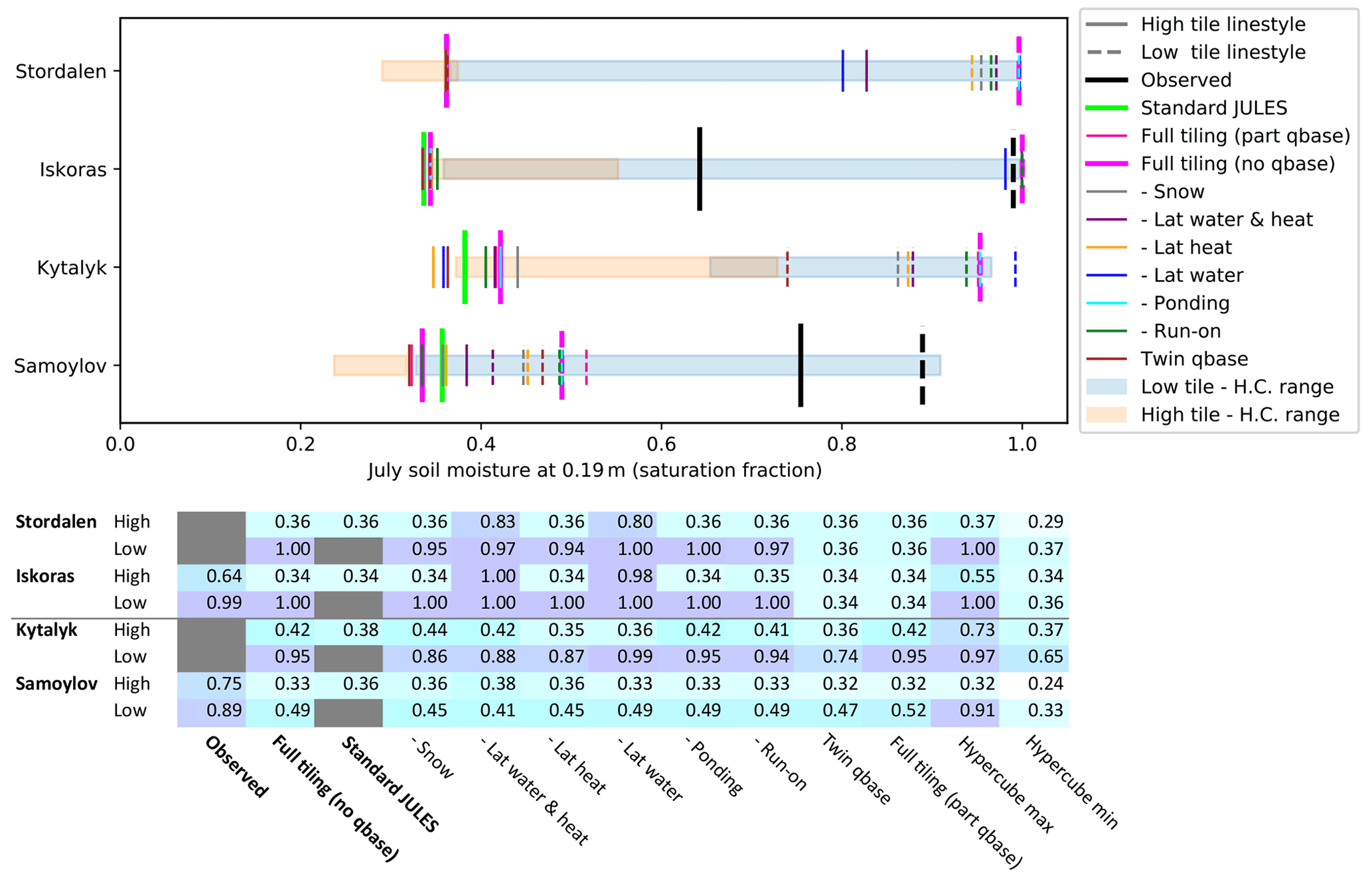
Figure 9Average July soil moisture (2000–2016) at 0.19 m for the subtractive process-switching runs, where model processes are switched off individually starting from the base configuration of full tiling (no qbase) (thick pink). Solid lines show the high tile, and dashed lines show the low tile. Observations are shown in black, standard JULES is shown in green. The range across the Latin hypercube sampling runs (H.C. range) are shown by the boxes. The depths of the observations are as follows: for Samoylov, the rim was at 0.22 m and the centre was at 0.23 m, and for Iškoras the palsa and mire were both at 0.2 m.
Changes in runoff and snowmelt water influx due to spatial variability in snow depth, run-on, and ponding therefore appear to be the main drivers of model soil moisture heterogeneity in this model, with lateral egress from the soil playing a role for palsa sites. Unsaturated soil-to-soil flows are generally negligible due to a combination of horizontally adjacent soil layers being saturated and/or frozen. While lateral unsaturated fluxes may have greater relative importance if the landscape drains or becomes drier, the hydrological difference between tiles would be less pronounced in this case anyway. This suggests that simpler, water-table-based models of lateral flow may be adequate in wetland environments.
3.2.3 Distinguishing the impacts of model processes on soil moisture
In order to directly attribute the effect of different model processes on soil relative saturation, a series of runs were performed where we took the main tiled model configuration (full tiling – no qbase) and switched off individual model processes in turn. These are the “subtractive process switching” runs referred to in Sect. 2.5.2. The resulting effect on the liquid fraction of saturation for the layer at 0.19 m depth is shown in Fig. 9. We find that although the individual effect of each process is small (aside from the effects of qbase and lateral flow from the high tile in palsa mire sites, as previously discussed), most processes have an effect in some conditions. We also find that the importance of different fluxes varies with the degree of saturation: for example, if the mire is well drained or already fully saturated, ponding will have little effect.
For polygons, switching off snow redistribution has one of the largest effects and reduces the liquid fractional saturation at 0.19 m by ∼0.05 to 0.1. Perhaps counterintuitively, for polygons, switching off lateral flows of heat (conductive and advective) has a larger effect than switching off lateral flows of water. Due to the shallow thaw depth, lateral flows of water are very small. Lateral flows of heat, however, are able to change the soil temperature, if only by a small amount (Fig. 12). This then has small knock-on effects on how much water is thawed in each layer, on the soil hydraulic conductivity, on infiltration, and on extraction of water by plants. Indeed, switching off lateral flows of water and heat together has the largest effect for Samoylov, reducing the splitting in level of fractional saturation from 0.2 to 0.06. It is interesting to observe that this effect is larger than that for switching off lateral heat alone, even though the process of switching off lateral flows of water on its own has a negligible effect. This is because the change in the thermal regime and consequent change in conductivity by switching off lateral flows of heat in this case enables a non-negligible amount of water flow, topping up the low tile saturation before winter. This example points to the situational dependence of the importance of model processes. Similarly, for Kytalyk, switching off lateral heat fluxes has the next largest effect after snow redistribution. This is perhaps unsurprising considering that for Kytalyk lateral flows of heat single-handedly reduce the temperature splitting from 2 ∘C to almost nothing (Fig. 12). Switching off runoff and ponding have little effect. However, when the opposite method is tried and aspects of the model are switched on individually using standard JULES as the base configuration (the “additive process-switching” runs), ponding and runoff can have a larger effect (Fig. B1, Appendix B), particularly after snowmelt. Once again, we see that model processes have different magnitudes of effect at different degrees of saturation.
For palsas, as we have already seen, drainage (qbase and lateral flows alike) is of key importance. Switching off lateral flows of water (blue) allows the high tile fractional saturation to increase dramatically from under 0.4 to over 0.8 at 0.19 m, while allowing qbase from the mire results in the opposite effect (“full tiling (part qbase)”, light pink) and the mire draining, resulting in the fractional saturation at 0.19 m of <0.38 (see also Fig. 7). For Stordalen, switching off lateral flows of heat, snow, and runoff serve to slightly reduce the fractional saturation of the mire (), but this effect is not seen for Iškoras.
3.3 Heat and temperature
3.3.1 The effect of microtopography on soil temperatures
The two types of microtopography have different effects on soil temperatures. Figure 10 shows the seasonal variation in modelled and observed temperatures, while Fig. 12 shows the observed and modelled soil temperatures for July at 0.19 m. The model shows a summer temperature splitting for palsa sites of 3.5 ∘C, which is smaller than the observed 5 ∘C, with the mean remaining lower and approximately unchanged compared with standard JULES. Polygons sites display small (0 to 0.5 ∘C) temperature splitting, in agreement with observations. Thaw depths are likewise similar for high and low tiles at polygon sites (Figs. 5 and 11), while palsa sites show a clear difference between palsa and mire. In the model, Iškoras shows signs of being on the edge of palsa degradation, with a talik forming for three consecutive winters after a warm summer in 2012 and greater winter snowfall for those years.

Figure 10Climatologies (2000–2016) showing the seasonal heterogeneity in soil temperatures at 0.19 m. Line styles show high and low tiles. Observations at this depth are not available for the polygon rim at Kytalyk and the palsa at Stordalen. “H.C.” indicates Latin hypercube sampling runs. The depths of the observations are as follows: for Samoylov, the rim was at 0.21 m, and the centre was at 0.2 m; for Kytalyk the rim was at 0.15 m, and the centre was at 0.25 m; for Iškoras, the palsa and mire were at 0.2 m; and for Stordalen the mire was at 0.25 m.
Figure 10 displays climatologies for soil temperatures at 0.19 m depth, showing that the model is able to reproduce the overall behaviour for both types of landscape over the course of a year. Year round, the observed differences in temperatures between the polygon rim and centre are comparatively small (<2.5 ∘C at 20 cm depth). However, polygon rims are observed to get colder in winter and be quicker to warm up in summer, can be warmer in summer, and are observed to cool down more quickly in winter. This general behaviour is reproduced in the tiled model, though the model lacks a substantial zero curtain in the autumn when re-freezing. This is probably due to the modelled polygon sites being too dry. Only the low tile of Kytalyk approaches having a substantial zero-curtain behaviour, partly due to it better reproducing an earlier build-up of snow but also due to it being the polygon tile nearest to the observed saturation. Microtopography tends to split temperatures so that they fall either side of that of standard JULES. If the temperature modelled by standard JULES lies outside of the observed temperature splitting and is greater or smaller, the temperatures modelled by the tiled run also tend to be biased in the same direction and greater or smaller, respectively. While polygon sites are close to observations in July, both standard JULES and the tiled configuration are generally colder than observed in summer, in addition to warming up and cooling down earlier. In addition to the aforementioned differences in soil moisture, part of the discrepancy in timing may be due to the shorter period of forcing data snowfall. That Samoylov is too cold in winter may be in part due to experiencing delayed snowfall. Palsa mires show a more pronounced splitting in temperature for both the summer and the winter than polygons, and the model captures both the difference in winter temperatures for Iškoras and the mire zero curtain well. However, the temperatures for both standard JULES and the tiled runs are too small in summer.
Modelled thaw depths are compared with observations in Fig. 11, and were diagnosed by linearly interpolating the position of 0 ∘C soil temperature closest to the surface. As with the soil temperatures, tiling causes a clear difference in thaw depths for palsa sites and little difference for polygon sites. It is helpful to compare these plots with the overview plots of soil temperature and unfrozen water in Figs. 5 and B6 (Appendix B). For the mire at Iškoras a clear talik can be seen, with the surface freezing to around 0.5 m in winter. For the modelled mire at Stordalen, while the 0 ∘C depth only just exceeds 1 m in summer, soil column temperature never drops far below 0 ∘C and at 0.5 m depth retains a substantial amount of liquid water year-round. While the tiled thaw depths for Iškoras are much closer to observations than for standard JULES, thawing is somewhat earlier than observed and 22 cm deeper for the high tile. A greater modelled ice content in the palsa, either through excess ice or a greater high tile saturation, could perhaps reduce this. For Samoylov, thawing in the model occurs 2–3 weeks earlier than observed. The model also shows a pronounced (∼ 15 cm) decrease in thaw depth between September and October before surface freeze-up, as opposed to the delayed decrease of soil temperatures observed. This again corresponds to the earlier snowmelt in spring and delayed build-up of snow in Autumn compared with observations (Fig. 6). This contributes to the maximum thaw depth in September being ∼ 15 cm smaller than observed.
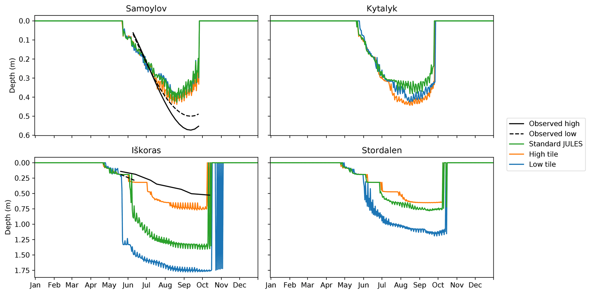
Figure 11Climatologies (2002–2016) of modelled vs. observed thaw depths. Observed thaw depths for Iškoras were from 2019, Samoylov CALM thaw depths were from 2002–2016, grouped according to classes 1 and 3 and averaged using a third-degree polyfit across transects.
In their paper implementing snow redistribution and lateral flows of water and heat in the E3SM Land Model (ELM)-3D v1.0, Bisht et al. (2018) simulated a transect across a low-centred polygon site in Barrow, Alaska. They found that the active-layer depth (ALD) was ∼ 10 cm shallower under rims and ∼ 5 cm greater under centres with snow redistribution on vs. the standard simulation. When lateral flows were also turned on (physics = 2D), ALDs were ∼ 7 cm deeper under rims and ∼ 2.5 cm shallower under centres than the standard simulation. Atchley et al. (2015) used a 1D version of the Arctic Terrestrial Simulator (ATS) also at Barrow that found ∼ 3 cm deeper thaw depths in centres and ∼ 0.3 cm deeper thaw depths in rims with snow redistribution turned on. In our simulation, we found ALDs for the tiled simulation were on average 1.1 and 6.1 cm deeper for the rim and 0.1 cm shallower and 4.3 cm deeper for the centre for Samoylov and Kytalyk respectively. While our simulations are not at Barrow, we note that our differences in the thaw depths for Samoylov are particularly small compared to the results of Bisht et al. (2018) and Atchley et al. (2015). We also see that together these authors similarly find that thaw depths in polygon centres can become shallower or deeper when microtopographic processes are switched on. In a similar manner to the smoothing effect of subsurface processes found by Bisht et al. (2018), in the sensitivity study in the next section we find that while snow redistribution causes colder high tiles and warmer centres, lateral flows of heat mean that much of this difference is cancelled out in summer. We also find that our choice of Δx is at a local minimum for Kytalyk, such that a small increase or decrease can lead to one tile or the other being warmer and having a greater ALD in summer.
In the previous section, we discussed that the introduction of ponding only has an effect on the level of soil saturation under certain conditions. For instance, if a pond is present, the soil may be fully saturated whether the pond is 1 cm or 1 m deep. Also, as mentioned in Sect. 2.3.4, currently the pond is purely a water store and lacks any thermal properties. This means that while Iškoras sometimes has a simulated pond depth of over 0.5 m, the soil temperatures are no different to if the pond was very shallow. As such, we expect the simulated temperatures to be more representative of a part of the landscape with shallow ponding. In future it would be beneficial to include the thermal effects of ponding, as we would expect the additional latent heat of the pond to cause a delay in soil freeze-up (Abolt et al., 2020; Langer et al., 2011), and even the formation of a talik at polygon sites if larger pond depths are simulated (Yi et al., 2014). This may require revisiting how the surface drainage of the pond is controlled (fpd) and possibly also the inclusion of additional tiles to ensure that both the wetland and permanently ponded areas of the grid cell are adequately represented. In this study, however, Iškoras is the only site for which a persistent pond forms. The other sites form only a temporary pond after snowmelt, so for these sites adding the thermal effects of ponding would not be expected to affect winter freeze-up.
3.3.2 Distinguishing the impacts of model processes on soil temperatures and quantifying heat fluxes
Figure 12 shows the effect on soil temperatures of the subtractive process-switching runs, where we took the main tiling configuration (“full tiling (no qbase)”, pink) and switched off model processes individually. These are the same runs as shown for soil moisture in Fig. 9. Out of the model processes shown, we see that snow redistribution and the effect of limiting drainage (qbase) have the largest effect for palsa sites, showing that both the increased depth of snow and a saturated lower tile are necessary for modelling the temperature splitting. It remains to be seen if the high tile would also get significantly warmer and more in line with observations if it too were wetter. While not shown here, on its own snow redistribution results in almost the full winter temperature splitting for palsa sites and too great a winter temperature splitting for polygon sites. The effect of snow redistribution on summer temperatures is smaller, but it is still responsible a large part of the temperature splitting.

Figure 12Average July soil temperature (2000–2016) at 0.19 m for the subtractive process-switching runs, where model processes are switched off individually starting from the base configuration of full tiling (no qbase) (thick pink). Solid lines show the high tile and dashed lines the low tile. The range across the Latin hypercube sampling runs (H.C. range) are shown by the boxes. The depths of the observations are as follows: for Samoylov, the rim was at 0.21 m, and the centre was at 0.2 m; for Kytalyk the rim was at 0.15 m, and the centre was at 0.25 m; for Iškoras, the palsa and mire were at 0.2 m; and for Stordalen the mire was at 0.25 m.
Comparing the “full tiling (no qbase)” run (pink) with the “full tiling – lat heat” run (orange), lateral heat conduction has the effect of reducing the temperature splitting by 0.6 to 1.1 ∘C for palsa sites and 1.1 to 2.0 ∘C for polygon sites. This eliminates almost the entire temperature splitting for Kytalyk. Looking at the average fluxes, these lateral flows of heat are almost entirely conductive rather than advective (Fig. B4, Appendix B). This may be due to the lack of saturated soil water fluxes in our model. The surface sensible and latent heat fluxes for the high and low tiles remain approximately the same as for standard JULES (Fig. B4, Appendix B), with low tiles having lower average sensible and net radiation fluxes than standard JULES and vice versa for the high tile. The modelled lateral heat conduction per unit length of border for Iškoras is 2.9 W m−1. Over a year, the energy transferred per metre of border could melt 0.28 m3 of ice. Interestingly, this is of the same order of magnitude as the 0.13 m3 yr−1 m−1 of volumetric loss of permafrost peat plateau edge found by Martin et al. (2021). Of course, not all the lateral heat flux would go into melting ice, and thus this rate of thaw would be smaller. Nevertheless, it suggests the possibility that the modelled heat flux between just two tiles could be used to calculate the rate of lateral thaw at the interface and hence the rate of areal change from one tile to the other.
The reduction in temperature splitting by the lateral flows of heat means that it is harder to see the effect of individual model processes for polygons by turning processes off individually. However, when looking at the additive process-switching runs (Fig. B2, Appendix B), small effects of the ponding and lateral flows can also be seen. Again, the effect of lateral flows of heat enabling lateral flows of water in polygons can also be seen, as adding lateral flows of water and heat has a larger effect than adding lateral flows of water alone. The amount that drainage, ponding, runoff, and lateral flows of water increase the summer temperatures of the low tile approximately follows that of their effects on soil moisture (Fig. B1 in Appendix B).
3.4 Methane
Figure 13 shows methane fluxes calculated using the observed soil carbon profiles combined with modelled soil temperatures from the “standard JULES” and “full tiling (no qbase)” runs. In this figure, standard JULES has qbase switched on while tiled runs have qbase off. This is to represent the difference in methane fluxes between how JULES is usually configured and a fully microtopographic approach. Based on the effect of the tiled model on temperatures seen in the previous section, we might expect to see a larger difference in methane production compared to standard JULES for the mire and little difference with respect to the polygon centres. Indeed, the total methane production for the polygons in JULES remains virtually unchanged for Samoylov and only 8 % or 9 % higher for Kytalyk. The palsa sites show an increase in methane fluxes vs. standard JULES of 9 % or 10 % using the non-microbial scheme (NM); however, when using the microbial scheme (M) for Iškoras this increases to 49 %. This is likely a factor of whether or not the microbes can survive or grow in all soil layers – for example, they are less likely to grow a population in permafrost soil layers. These results show that explicitly modelling microtopography can increase modelled methane fluxes vs. standard JULES in cases where microtopography-driven processes enable sufficiently different soil thermal and hydrological conditions to coexist. As previously mentioned, here we have used the observed (rather than modelled) soil carbon profiles to calculate the methane flux. In reality, the carbon substrate might also be greater in the wet parts of the landscape compared to the landscape average (Wagner et al., 2003; Eckhardt et al., 2019), and thus the effect on simulated methane that we show here may be amplified when soil carbon dynamics are modelled.
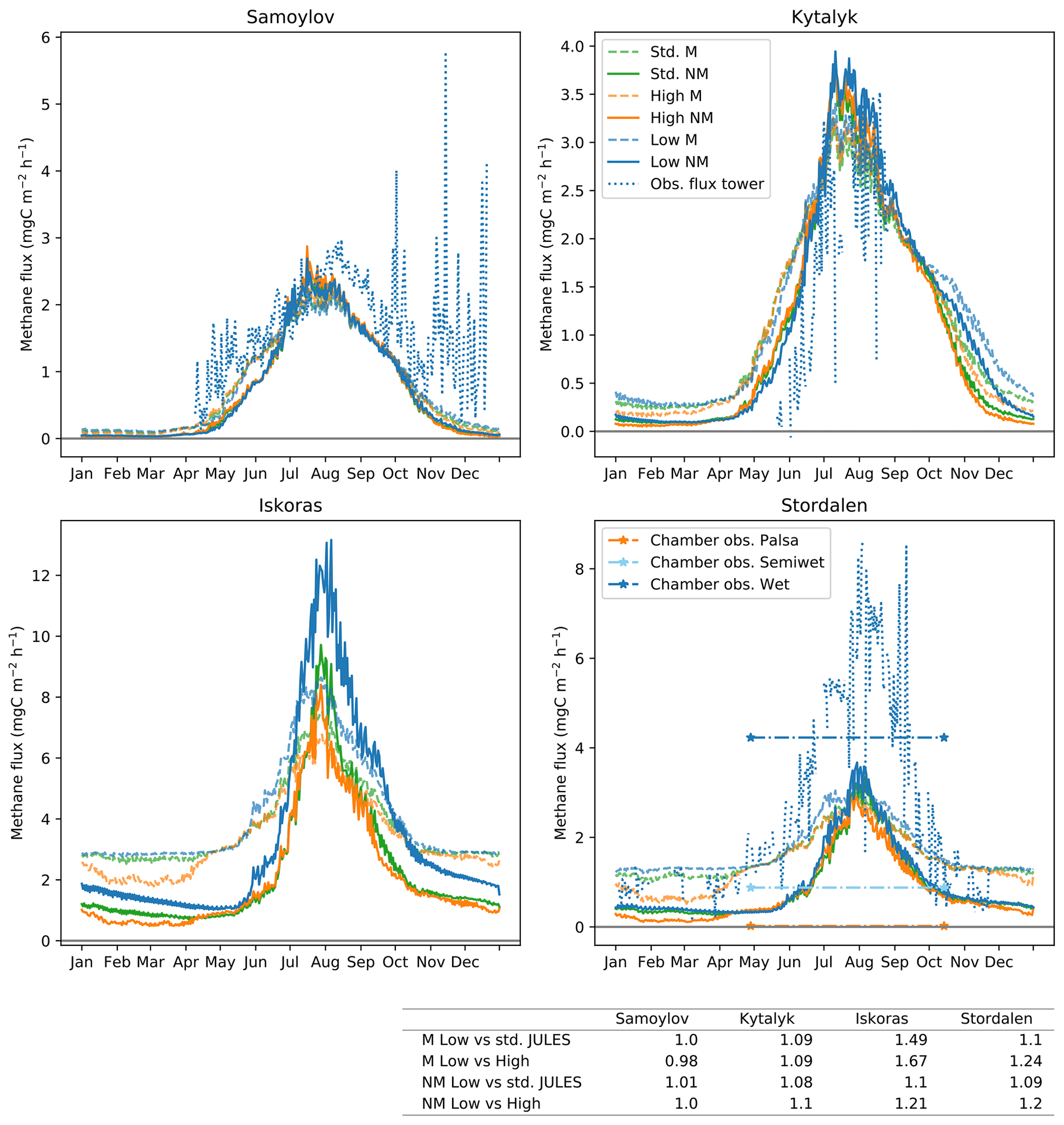
Figure 13Climatology (2000–2016) of diagnosed methane fluxes calculated using modelled soil temperatures and observed soil carbon profiles, comparing fluxes from standard JULES and the low tile. Diagnosed methane fluxes for the high tile are shown for comparison only, as the drier soil would inhibit methane fluxes from these tiles. M is used to indicate the microbial methane model, and NM is used to indicate the non-microbial methane model. Methane chamber measurements for Stordalen are for 2002–2007 for the green season (days 119–288) and indicate the variability in methane fluxes due to hydrological conditions and thaw present at the site (Bäckstrand et al., 2010). Here, standard JULES has qbase switched on while tiled runs have qbase off.
When comparing the simulated fluxes with flux tower observations (dotted lines in Fig. 13), fluxes show reasonable agreement for palsa sites, though they are slightly lower than those observed for Samoylov but are more significantly lower than those observed for Stordalen. This is what could be expected due to average modelled low tile summer temperatures for July and August being <1∘C lower than observed for polygons, but >4 ∘C lower for palsa sites (Fig. 10). Previous modelling using a standard version of JULES with the modification of a saturated soil column has been able to better reproduce the observed flux tower methane emissions for Stordalen (Chadburn et al., 2020, Fig. 3). This underlines the primary importance of the core model setup in accurately modelling methane emissions and that the difference made by modelling microtopography is only a refinement to this. In this case, the difference may be that the very upper layers of the lower tile in the model do not remain saturated year-round (Fig. 7) unlike the fully saturated column in Chadburn et al. (2020). This drier surface layer of soil provides an insulating effect, meaning that the soil does not heat up as much in summer. For the full tiling (no qbase) runs, Stordalen's pond is only seasonal, developing after snowmelt and disappearing before midsummer. In contrast, Iškoras has a persistent pond and a fully saturated lower tile, resulting in higher summer temperatures and methane fluxes more comparable to those observed for Stordalen.
While eddy covariance methane observations (EC obs.) have the benefit of providing a detailed time series and a landscape aggregate, they do not resolve small-scale variations. For Fig. 13, in order to compare the EC obs. with the modelled fluxes for the lower tile, for Kytalyk and Stordalen the EC obs. were selected for when the tower footprint was over the wetter area of the landscape, while for Samoylov the fluxes were divided by the observed wetland fraction (Table A2, Appendix). Chamber measurements are able to resolve these spatial variations; however, it is harder to get a landscape-scale average, and measurements often lack an extended time series. The average simulated fluxes are within the ranges of chamber flux measurements for Samoylov (2.7±1.3 mgC m−2 h−1, Sachs et al., 20101) and for Kytalyk (3±2 mgC m−2 h−1, Huissteden et al., 20052) though these are not shown in Fig. 13 due to the lack of a multi-year average. Methane chamber measurements from Bäckstrand et al. (2010) are shown for Stordalen. These measurements are the average from 2002–2007 for the “green season” (days 119–288). Chamber measurements have been grouped as in Johansson et al. (2006); Bäckstrand et al. (2010), where the semi-wet area (three chambers) corresponds to Sphagnum spp. and Carex spp. and the wet area (two chambers) to Eriophorum angustifolium. Three chambers were used for the palsa micro-site. The wet area is completely saturated and permafrost free. The semi-wet area has a water table fluctuating within 20 cm of the surface, and while this area not raised like the palsa, it is only partially thawed. A large difference in methane emissions can be seen between the wet and the semi-wet areas. Our modelled lower tile fluxes are hard to directly compare with these areas. The lower tile sits in between the two in terms of moisture and arguably in terms of temperature (based on thaw depths), and thus the methane fluxes could be approximately correct for an area of the mire that is between wet and semi-wet. However, as the saturated areas contribute a much larger share of the total methane emissions (see, e.g. orange vs. blue horizontal lines in Fig. 13d), simulating methane emissions from unsaturated parts of the landscape will have little impact on the upscaled fluxes.
Another problem for upscaling is that the method of calculating methane emissions used here is now decoupled from changes in the water table. In reality, the thickness of the oxic layer determines the amount of substrate unavailable to methanogens and affects how much of the generated methane is oxidised. This is represented in standard JULES by varying the wetland fraction depending on the water table level, as described in the introduction. Here, the low tile area is fixed, and so our calculation of the fluxes will increasingly be an overestimate as the water level drops below the surface. Future versions of the model will therefore require changes in the water table and the methane fluxes to be linked. As Chadburn et al. (2020) observe, doing so would enable the microbial dynamics to be better modelled, as methanogens would be unable to survive in layers where the saturation is varying rapidly. Adding water table dynamics would also add to the feedback on the methane fluxes of the insulating dry layer described previously that limits summer soil temperatures, making the low tile emissions more sensitive to changes in the water table. This is again a contributing factor to the observed spatial variability in methane emissions and must be considered when upscaling.
3.5 Sensitivity study
The sensitivity study investigated the response of the model to varying model parameters using the methods described in Sect. 2.5.2. Using the estimated possible ranges of parameter values, we determined the range of possible modelled soil temperatures for each site and quantified how the uncertainty in model parameters affects the uncertainty in model output. These tests are important as they confirm that the model will not give unreasonable results if the parameters are set differently, while also indicating which parameters are in most need of constraining.
Figures 10 and 12 show the variability in the temperature splitting (TS, the difference between high and low tile temperatures) for July at 0.19 m as a result of varying model parameters using Latin hypercube sampling (LHS). It can be seen that this variability is comparable to the size of the observed TS itself. For the polygonal sites, the choice in parameters can result in the TS being larger by up to ∼3 ∘C, as the usual splitting is small (0.5 ∘C for Samoylov). A similar increase from the usual modelled splitting is also possible for the palsa sites; however, as the modelled TS is already smaller than observed, the resulting splitting can only be up to ∼1.5 ∘C larger than observed. The parameter ranges used for the LHS are generous, and thus we can be confident that including microtopography is “safe” and will not result in unreasonable modelled temperatures. However, that the variability in the TS is similar to the size of the modelled TS means that care must be taken when choosing parameter values.
Table 5 gives approximate estimates of parameter uncertainties by site, which were then used alongside the results from the individually varying parameter runs (as in Fig. C1c, Appendix) to find the resulting effects of the parameter uncertainties on the size of the July TS at 0.19 m depth. The parameter uncertainties are our estimates of the uncertainty in the parameters used and not a quantification of site-level variability based on any large-scale survey. They should therefore be treated as a guide, but they nevertheless remain adequate for their use here in identifying the main sources of uncertainty in the model output. Furthermore, rather than basing our analysis purely on the numerical results given in Table 5, we also examined the individual plots of how the output temperature varies with each parameter across the range given in Table 2 (as in Fig. C1c) to avoid a small underestimation of the parameter uncertainty being unknowingly responsible for a large underestimation of output uncertainty. Uncertainties in spatial parameters for polygons were estimated using the digital elevation map for Samoylov (Boike et al., 2019). Uncertainties in the spatial parameters for Palsa sites are based on how far the assumptions made in determining the parameters could be stretched, namely the choice of palsa elevation from the observed range and the chosen geometry of bordering squares (see Sect. 2.5.1). The uncertainty in the snow catch sc was based on our estimate of the usual variability in plant growth atop these landforms and corroborated by observed snow depths on the raised areas at Samoylov and Iškoras. The uncertainty in fpd, fd1, fd2 and fro indicates our uncertainty in how the processes these parameters represent operate in real life. For example, based on the digital elevation map of the low-centred polygons at Samoylov, we assume that most of the potential runoff from the rim ends up in the centre, but it may be that only around half ends up there if equal proportions of the rim slope towards and away from the centre.
Table 5Estimated parameter values (value) and uncertainties (±) by site, and the resulting effect of the parameter uncertainty on the size of the July temperature splitting at 0.19 m depth (effect). indicates whether increasing the parameter causes the temperature splitting to increase (1) or decrease (−1) or whether it indicates the presence of local maxima (0+) or minima (0−).
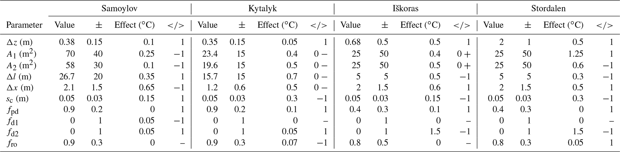
For Kytalyk, our choice of parameters appears to have resulted in a local minimum for the TS, such that for four of the parameters, variation in either direction results in an increase of magnitude of the TS. As a result, either tile could become the warmer tile, and thus microtopography could either increase or decrease the fluxes. The largest resulting change in the TS as a result of the uncertainty in an individual variable is 1.5 ∘C for the palsa sites and 0.7 ∘C for the polygon sites. This can be a large fraction of the overall TS and is larger than the effect of many of the individual model processes, reinforcing the need to carefully choose model parameters. This is particularly the case for A1 (the high tile area, which affects the depth of snow on the low tile), fd1 (fraction of drainage from the low tile, which has been previously discussed), and Δx (the horizontal distance, which is hard to measure but effects the magnitude of lateral fluxes). At the other end of the scale, uncertainties in the values of fpd (maximum pond depth), fd1 (drainage from high tile), and fro (run-on fraction) have little individual effect (C) on the TS. There can be a large variability in palsa heights at an individual site, for instance, Olefeldt and Roulet (2012) record a range of 0.5 to 2 m for Stordalen. It had therefore been a concern that a single pair of tiles may not be representative if this also corresponds to a large variability in temperature. However, Fig. C1c shows that there is little change in the modelled temperatures once the palsa elevation is above 0.5 m, meaning that having only two tiles can be a valid representation of multiple palsas whose heights are above this threshold. While we have taken care in choosing model parameters based on observations, it is recommended parameter validation be implemented for future users so that unreasonable or even unphysical combinations of parameters are not allowed. The sensitivity study also provides further motivation for a dynamic representation of the parameter Δx, as this currently responsible for a 0.6 ∘C uncertainty in the TS.
The results of the individually varying parameters runs also give insight into the effect of varying parameters on winter soil temperatures and particularly the model response to parameters affecting the snow scheme. While the main behaviours follow directly from the model of Eqs. (1) and (2), it is worth noting that soil temperatures are most affected by changes in snow depth when snow depths are shallower. For instance, soil temperatures are highly sensitive to the snow catch parameter (sc) for the high tile, where the sensitivity tests show that a difference of 5 cm can result in as much as 2 ∘C difference in winter soil temperatures at 0.19 m (Fig. C1b, Appendix). However, the same is not true of the response of the low tile temperatures to snow catch where the snow is deeper, and thus changes have less effect. Similarly, changes to A1 (the area of box 1) are a key control on snow depths on the low tile and can affect the snow depth by a much greater amount but affect the temperature less. For instance, changing the A1 by 50 m2 for Stordalen results in changing the low tile snow depth by around 0.5 m and a temperature increase of around 1 ∘C.
In this study we have constructed and tested an explicit representation of microtopography within the JULES land surface model. We have followed a two-tile approach as suggested by Aas et al. (2019) and Nitzbon et al. (2019), although in order to implement such a model in JULES we have taken a different approach to implementing lateral fluxes, runoff, and ponding. Our purpose has been to test the efficacy of an explicit representation of microtopography further by comparing the model output with observations of snow depth, soil moisture, and temperature at additional sites; through the study of the model's behaviour and uncertainty through testing a range of parameter values; and through gauging the impact of modelling microtopography on modelled methane fluxes. We have shown that a simple two-tile representation of microtopography (Fig. 2) is able to improve modelled snow depths (Fig. 6), soil moisture (Fig. 7), and temperatures (Fig. 10) in JULES for four sites and that this can lead to an increase in the modelled methane fluxes vs. standard JULES in some cases. These changes would affect the results of modelling the northern high latitudes in their current state, though they have implications for (and will be affected by) future landscape changes due to ground ice thaw and changes in wetland area. The increase in methane fluxes was only appreciable for the palsa and mire sites (+10 % to 49 %, Fig. 13) due to the small difference in temperatures between tiles at the polygon sites (Fig. 10). We hypothesise that a similar effect on methane fluxes would be seen for other wetlands in the discontinuous permafrost region. This is because the model processes are general to all forms of microtopography and because through this study we have found a weak dependence of soil temperatures on elevation differences greater than 0.5 m (Fig. C1c, Appendix). To test this hypothesis would require data from additional sites, so this study underlines the need for more microtopographically resolved data to be available.
Palsa mires are by their nature found in marginal locations where the transition between permafrost and non-permafrost can be seen. That explicitly modelling microtopography has a greater effect on the modelled fluxes at these sites is unsurprising due to the distinct nature of these conditions which cannot coexist in standard JULES. Future studies should investigate the potential difference to the modelled area of permafrost and methane production when a tiled approach to microtopography is applied at the pan-Arctic scale. The marginal nature of palsa mires also makes them sensitive to climate fluctuations (Seppala, 2006). Palsa degradation has been observed at these two sites and more broadly across Europe and western Siberia (Kirpotin et al., 2011; Borge et al., 2017), with one study projecting that over half the area currently suitable for palsas in Fennoscandia is very likely become unsuitable by the 2030s (Fronzek et al., 2010). The changing climate in these areas could be increasing the difference in conditions between permafrost and mire while palsas are still present but are being pushed out of their climate envelope of stability. This motivates modelling microtopography for the purpose of understanding the future effects on methane fluxes of new areas experiencing permafrost degradation.
Snow depth was a key control on the modelled soil temperatures of each tile (Fig. 12). Despite its simplicity, the snow scheme performed well at the modelled sites (Fig. 6). While these sites are representative of widespread landforms, it remains to be seen if the scheme would perform as well in sites where the microtopography does not show such clear small-scale repetition. Investigating the impact of linking the snow catch parameter to the vegetation height is a key next step and will be important for modelling snow–vegetation feedbacks. The impact of microtopography on modelled plant communities was not examined in this study as work needs to be undertaken to implement plant functional types in JULES that are more representative of Arctic plants and their variety and that have the correct response to saturated soils. The ability to model different plant functional types in microtopographically distinct areas would, however, be interesting with respect to peat formation and the effect of different plant functional types on methane emissions (Cooper et al., 2017; Rupp et al., 2019). Combining this model with the ability to model peat formation as in Chadburn et al (2022a) could lead to interesting dynamics as the tile elevations change, and would enable the future of features such as drained thermokarst lake basins to be modelled.
This study reiterates that making wetlands wet is a clear requirement for accurate representations of soil temperatures and therefore methane emissions from high-latitude wetlands (Fig. 12). An explicitly modelled wetland “tile”, even if purely to provide more accurate soil temperatures for calculation of methane emissions, could therefore be a worthwhile step forward from models where grid cell soil temperatures are spatially homogeneous. Differences in the snowmelt, lateral drainage and runoff between tiles, and ponding on the low tile, were instrumental in modelling the effects of microtopography on hydrology. As such, it is difficult to suggest any of these processes that could be readily eliminated. However, several aspects of the hydrology were identified that require consideration for future modelling. While much of our effort was directed at modelling unsaturated flows, it was found that these fluxes played only a small part in modelling these wetland environments. Where lateral fluxes were appreciable, they were usually from a saturated layer to an unsaturated one (Fig. 8). Modelling the lateral fluxes based on the position of the water table may therefore provide an acceptable basis for a simplified implementation of these flows, and one which may better model advective flows of heat. The amount of drainage modelled from the low tile has a large effect for the palsa mires (Figs. 7, C1a). However, the current implementation of baseflow in JULES is not very suitable for a microtopographic model and also does not represent water influx, which is important for some wetlands. Consideration therefore needs to be given as to how the landscape-scale lateral flow out of and into wetlands could best be modelled. To allow for changes in the soil wetness, the methane flux calculation will need to be linked to the water table depth, which will also enable methanogen microbial dynamics to be better modelled. This will increase the sensitivity of the methane flux to the water table depth that is already present due to the effect of soil moisture on soil temperatures. This sensitivity is part of the reason for the observed spatial variability of methane emissions from wetter areas. There is therefore a question of how upscaling the methane fluxes from those calculated for the low tile can be done in a representative way. Bechtold et al. (2019) suggest that for peatlands the TOPMODEL formulation of calculating the distribution of the water table should be replaced with a normal distribution based on the microtopographic variability, alongside other modifications to the hydrology. This distribution could then be used alongside temperatures of tiles of different wetness to better represent the emissions from the whole of the mire. An alternative would be to explicitly represent the hydrological gradient using a larger number of tiles and/or a representation of hillslopes (Nitzbon et al., 2021; Swenson et al., 2019; Hazenberg et al., 2015). Both of these approaches could also provide a route to better modelling the landscape- or catchment-scale baseflow. Currently the model does not include a treatment of surface waterbodies beyond being a simple surface store, for which an additional pond or lake tile would be beneficial, as in Langer et al. (2016). Using a greater number of tiles may also be useful for the modelling of more complex features, for example by using three tiles to represent the centre, rim, and trough in a polygonal landscape (Nitzbon et al., 2019) or areas of land, wetland, and lakes (Schneider von Deimling et al., 2015). Indeed, Nitzbon et al. (2021) take this further, connecting multiple polygon units together to represent landscape-scale drainage and mesotopography.
Modelling microtopography provides a foundation for representations of thermokarst in Earth system models (Nitzbon et al., 2021) and for answering key scientific questions about the impact of abrupt thaw processes on emissions and the future extent of wetlands. Scaling to a pan-Arctic model requires consideration of how model parameters such as tile areas and elevations can be assigned on this scale, and a representation of thermokarst requires a model of how these parameters can change over time. This study provides motivation for it being possible to assign parameters that are representative at scale but also a measure of the uncertainty as a result of estimating these parameters. In particular, we find that within the expected ranges at these sites most parameters result in an associated uncertainty in July soil temperatures at 20 cm depth of under 0.8 ∘C, while the effect of the uncertainty in the high tile area and in the fractional drainage from the low tile result in an uncertainty on these temperatures of under 1.6 ∘C (Table 5). We also find a relatively weak dependence of summer soil temperatures on elevation difference within the expected ranges at each type of site. It would therefore be reasonable to associate a given elevation difference with a particular landform. Previously, thaw models based on the thawing of excess ice and subsequent vertical elevation change have been used to simulate the future evolution of polygonal landscapes and palsas or peat plateaus (Langer et al., 2016; Aas et al., 2016, 2019; Nitzbon et al., 2019; Cai et al., 2020; Martin et al., 2021; Nitzbon et al., 2021). These approaches are particularly suited to polygonal landforms where the relative elevations of tiles determine the transformation between low-centred and high-centred polygons, affecting the hydrology of these landscapes (Nitzbon et al., 2019, 2020, 2021). However, for areas of peat plateau (and for the expansion of thermokarst lakes) it may be more suitable to consider an area-based lateral thaw approach as this may require fewer tiles. We note that the modelled lateral heat conduction between tiles for Iškoras corresponds to melting 0.28 m3 of ice per year per metre of palsa–mire border, which is of the same order of magnitude as the 0.13 m3 yr−1 m−1 of volumetric loss of permafrost peat plateau edge found by Martin et al. (2021), indicating that such an approach may work. Recently, remote sensing and machine learning tools have enabled the mapping of the location and areas of different permafrost landforms for large regions, and the mapping of how these are changing (Nitze et al., 2018). At the same time, climate envelope models have allowed for pan-Arctic assessment of climatic suitability for palsas (Fewster et al., 2020) and ice wedge polygons and which areas may be subject to change in the future. These data will enable microtopographic models to be initialised and provide a basis for model evaluation. The time is therefore ripe for explicit representations of microtopography to be set up and assessed on a pan-Arctic scale.
Table A1Further site information. Acronyms are defined as follows: MAAT stands for mean annual air temperature, MAP stands for mean annual precipitation, WM stands for warmest month, and CM stands for coolest month. Other than “recent MAAT”, climatic variables are aggregated for the period given by “variable period”.
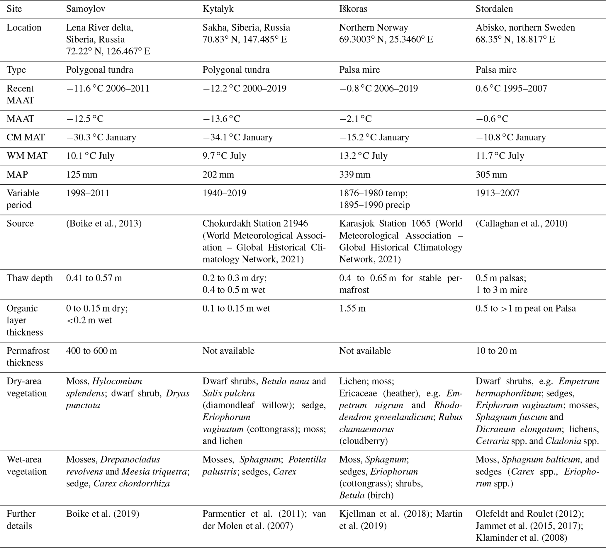
Table A2Sources of site observations.

* Wetland fraction used for scaling eddy covariance data to flux per square metre from Chadburn et al. (2020)

Figure B1Average July soil moisture (2000–2016) at 0.19 m for the additive process-switching runs, where model processes are switched on one at a time starting from the base configuration of standard JULES (light green). The depths of the observations are as follows: for Samoylov, the rim was at 0.22 m and the centre was at 0.23 m, and for Iškoras the palsa and mire were both at 0.2 m.
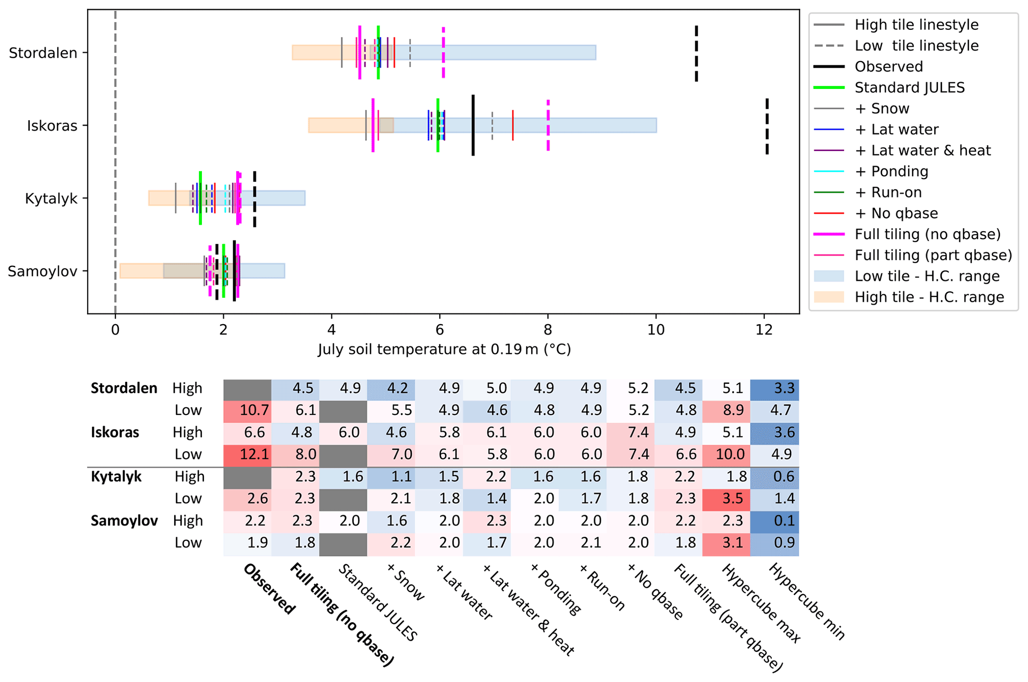
Figure B2July soil temperature (2000–2016) at 0.19 m for the additive process-switching runs, where model processes are switched on one at a time starting from the base configuration of standard JULES (light green). The depths of the observations are as follows: for Samoylov, the rim was at 0.21 m, and the centre was at 0.2 m; for Kytalyk the rim was at 0.15 m, and the centre was at 0.25 m; for Iškoras, the palsa and mire were at 0.2 m; and for Stordalen the mire was at 0.25 m.
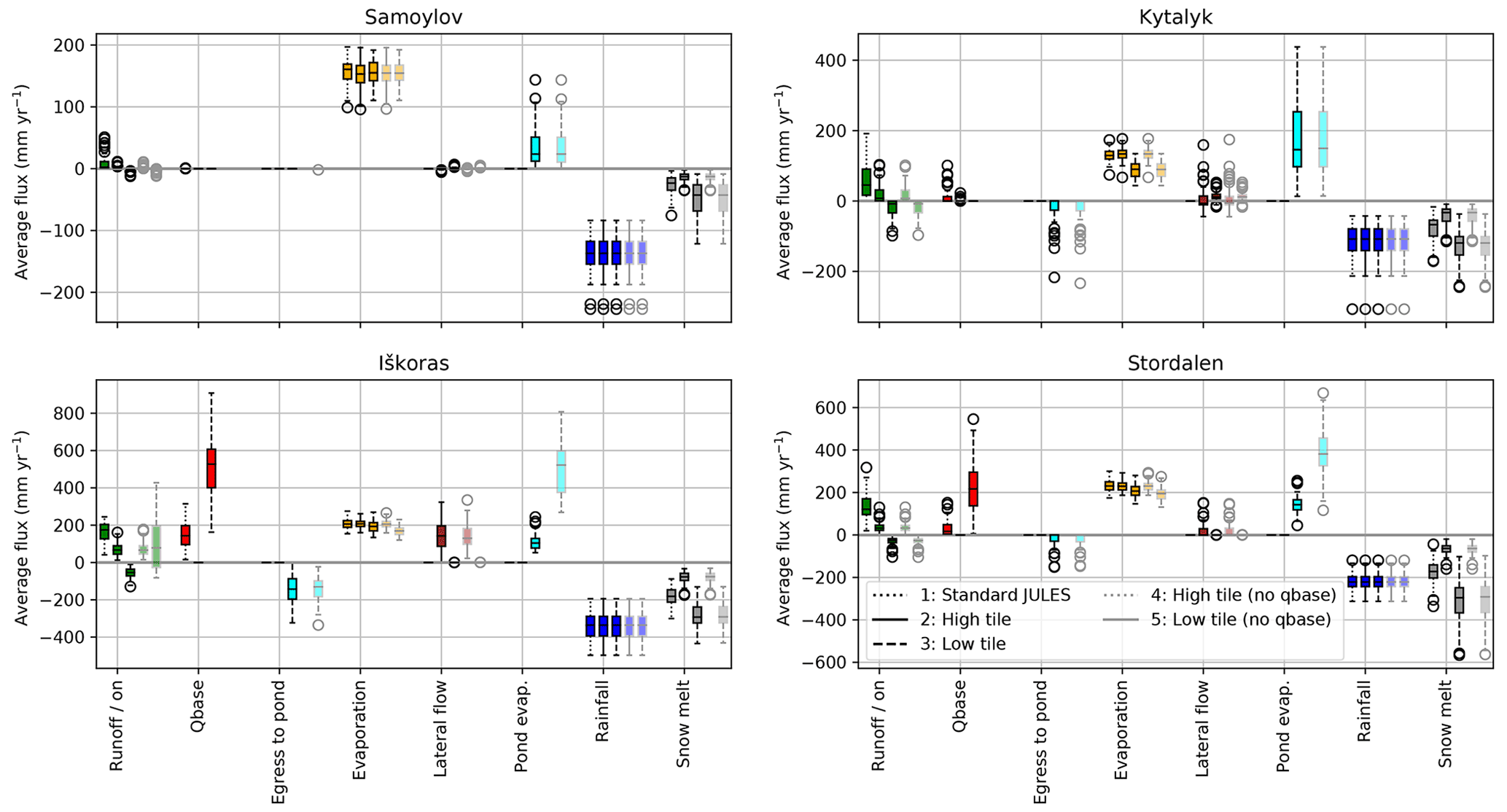
Figure B3Average yearly simulated moisture fluxes for the period 1950–2016 for all sites with the qbase on configuration. Fluxes for the qbase off configuration (as in Fig. 8) are shown in grey for comparison.

Figure B4Average yearly simulated energy fluxes (1950–2016) for all sites with the qbase on configuration. Fluxes for the qbase off configuration are shown in grey for comparison.
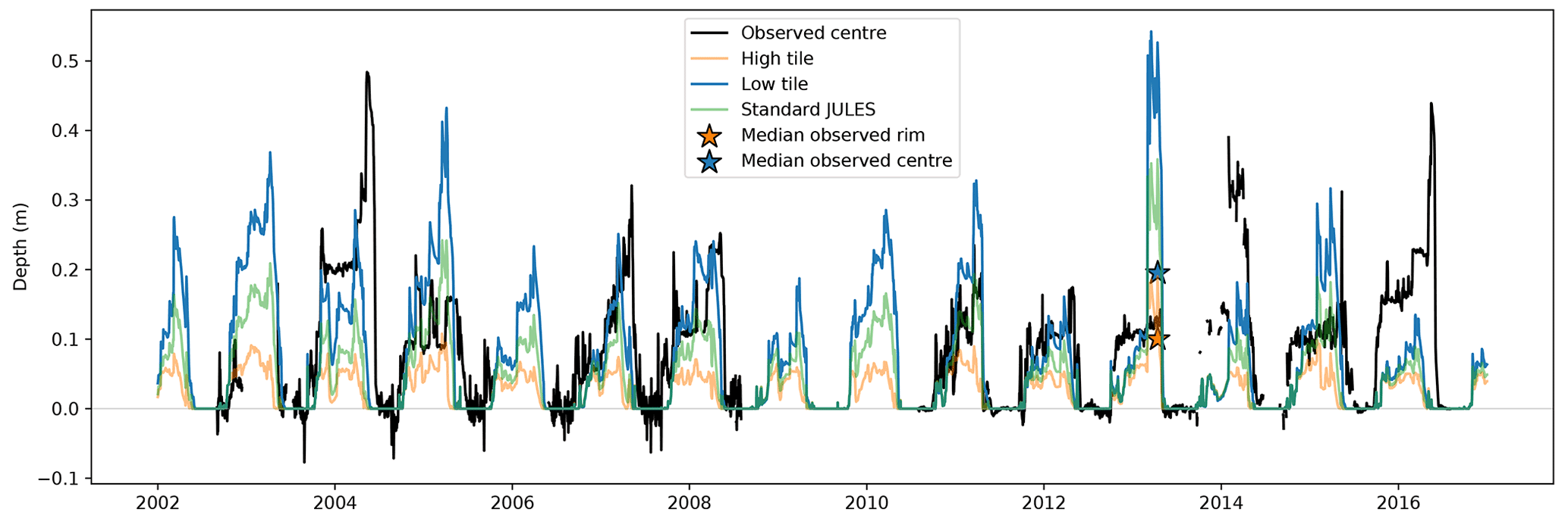
Figure B5Time series comparing observed and modelled snow depths for Samoylov showing inter-annual variability in snowfall. Snow depths have been bias-corrected using the signal during the snow-free season. Stars denote the median observed value across multiple polygons by Gouttevin et al. (2018) on their campaign in April 2013.
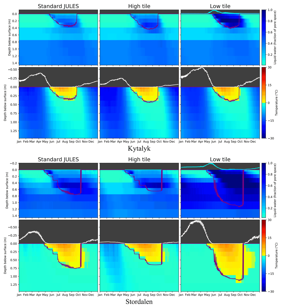
Figure B6Climatologies (2002–2016) providing a comparison of observations with standard and tiled (no qbase) JULES for the polygon site Kytalyk and the palsa site Stordalen. The white line above the plots of soil temperature shows simulated snow depth, the cyan line above the plots of simulated soil moisture shows simulated pond depth, and the purple line shows thaw depth.
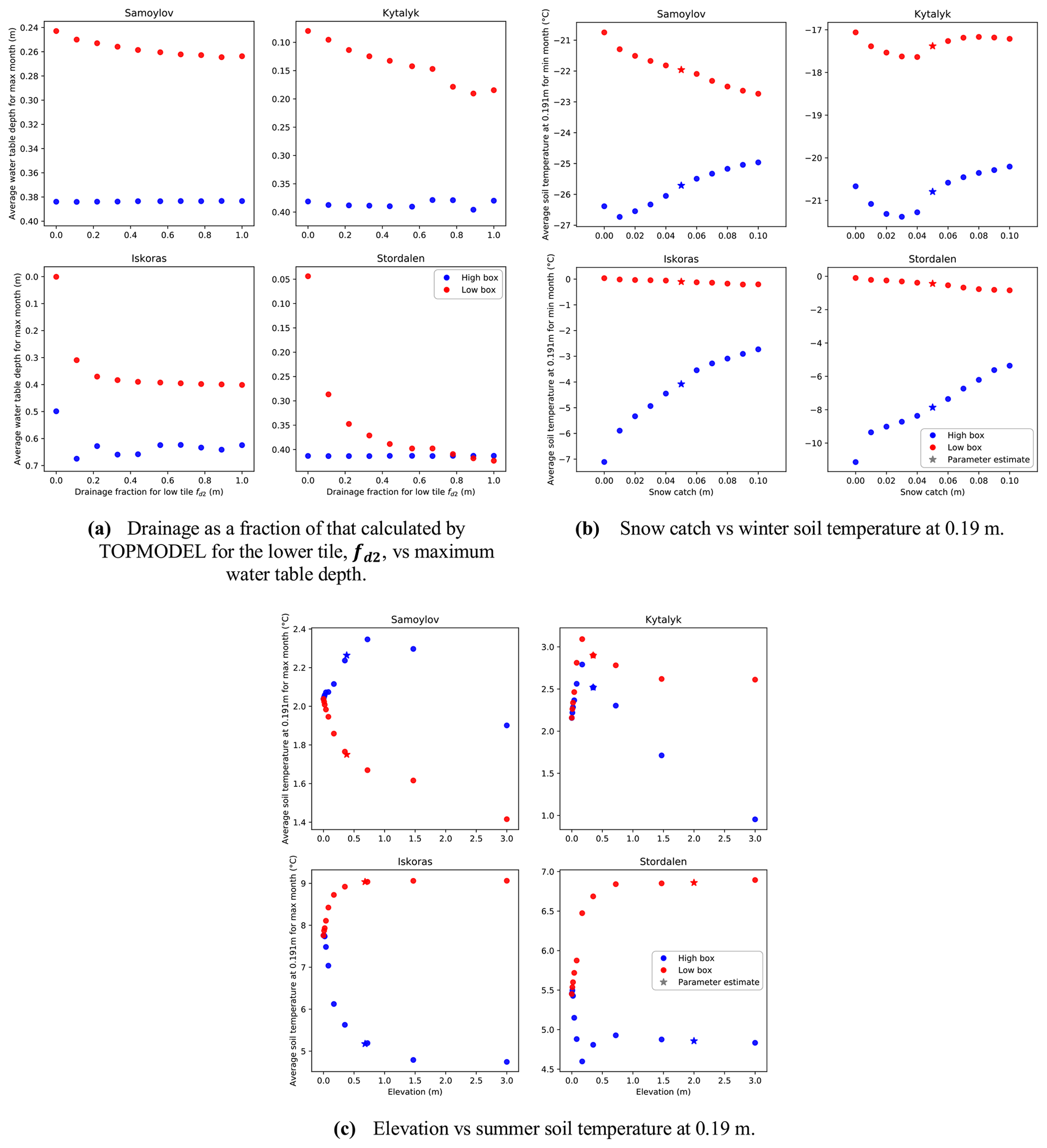
Figure C1Selected results from the varying individual parameter runs, showing an output variable against the parameter being varied. Red and blue show the high and low tiles, respectively. Panels (b) and (c) have qbase off for both tiles.
Model code and Rose suite configuration files are freely available from the Met Office Science Repository Service (https://code.metoffice.gov.uk/ last access: 20 April 2022) upon registration and completion of a software licence. Details on accessing and running JULES configurations can be found in Wiltshire et al. (2020). The tiled model code (vn5.4_microtopography) can be found at https://code.metoffice.gov.uk/svn/jules/main/branches/dev/noahsmith/r17292_vn5.4_lateral_9box (revision 20192; Smith and JULES collaboration, 2022a, registration required), which is itself a branch from a modified version of JULES 5.4 (https://code.metoffice.gov.uk/svn/jules/main/branches/dev/sarahchadburn/vn5.4_microbial_ch4, revision 15781; Chadburn et al., 2022b, registration required). Tiled model runs use Rose suite u-bo877x (https://code.metoffice.gov.uk/svn/roses-u/b/o/8/7/7/, Smith and JULES collaboration, 2022b, registration required), which was built off of the base configuration u-an231 (“standard JULES”) (https://code.metoffice.gov.uk/svn/roses-u/a/n/2/3/1/, revision 175882; Burke and JULES collaboration, 2022, registration required). Further configuration files for sensitivity suites can be found at https://doi.org/10.5281/zenodo.6476233 or https://github.com/noahdsmith/JULES_microtopography_model_rose_suites/ (last access: 20 April 2022) (Smith and JULES collaboration, 2022). Model output, processed observational data, and plotting code are available at https://doi.org/10.5281/zenodo.5565162 (Smith et al., 2021). Sources for site observations can be found in Table A2.
The supplement related to this article is available online at: https://doi.org/10.5194/gmd-15-3603-2022-supplement.
NDS developed the model, performed simulations, and wrote the first version of the manuscript. EJB prepared forcing data and set up the JULES suite u-an231. SEC, EJB, RHT, and HR contributed to model development. SEC, JB, SW, HL, CTC, BE, TF, KSA, and IHJA provided model forcing and evaluation data. All authors contributed to the text of the manuscript.
The contact author has declared that neither they nor their co-authors have any competing interests.
Publisher's note: Copernicus Publications remains neutral with regard to jurisdictional claims in published maps and institutional affiliations.
In addition to those mentioned in Table A2, we thank Han Dolman from the Department of Geosciences at the VU University Amsterdam for contributing methane and soil temperature data for Kytalyk.
This paper was edited by David Lawrence and reviewed by two anonymous referees.
Aas, K. S., Gisnås, K., Westermann, S., and Berntsen, T. K.: A Tiling Approach to Represent Subgrid Snow Variability in Coupled Land Surface–Atmosphere Models, J. Hydrometeorol., 18, 49–63, https://doi.org/10.1175/JHM-D-16-0026.1, 2016.
Aas, K. S., Martin, L., Nitzbon, J., Langer, M., Boike, J., Lee, H., Berntsen, T. K., and Westermann, S.: Thaw processes in ice-rich permafrost landscapes represented with laterally coupled tiles in a land surface model, The Cryosphere, 13, 591–609, https://doi.org/10.5194/tc-13-591-2019, 2019.
Abolt, C. J., Young, M. H., Atchley, A. L., Harp, D. R., and Coon, E. T.: Feedbacks Between Surface Deformation and Permafrost Degradation in Ice Wedge Polygons, Arctic Coastal Plain, Alaska, J. Geophys. Res. Earth Surf., 125, e2019JF005349, https://doi.org/10.1029/2019JF005349, 2020.
Åkerman, H. J. and Johansson, M.: Thawing permafrost and thicker active layers in sub-arctic Sweden, Permafr. Periglac. Process., 19, 279–292, https://doi.org/10.1002/ppp.626, 2008.
Atchley, A. L., Painter, S. L., Harp, D. R., Coon, E. T., Wilson, C. J., Liljedahl, A. K., and Romanovsky, V. E.: Using field observations to inform thermal hydrology models of permafrost dynamics with ATS (v0.83), Geosci. Model Dev., 8, 2701–2722, https://doi.org/10.5194/gmd-8-2701-2015, 2015.
Bäckstrand, K., Crill, P. M., Jackowicz-Korczyñski, M., Mastepanov, M., Christensen, T. R., and Bastviken, D.: Annual carbon gas budget for a subarctic peatland, Northern Sweden, Biogeosciences, 7, 95–108, https://doi.org/10.5194/bg-7-95-2010, 2010.
Bechtold, M., Lannoy, G. J. M. D., Koster, R. D., Reichle, R. H., Mahanama, S. P., Bleuten, W., Bourgault, M. A., Brümmer, C., Burdun, I., Desai, A. R., Devito, K., Grünwald, T., Grygoruk, M., Humphreys, E. R., Klatt, J., Kurbatova, J., Lohila, A., Munir, T. M., Nilsson, M. B., Price, J. S., Röhl, M., Schneider, A., and Tiemeyer, B.: PEAT-CLSM: A Specific Treatment of Peatland Hydrology in the NASA Catchment Land Surface Model, J. Adv. Model. Earth Syst., 11, 2130–2162, https://doi.org/10.1029/2018MS001574, 2019.
Best, M. J., Pryor, M., Clark, D. B., Rooney, G. G., Essery, R. L. H., Ménard, C. B., Edwards, J. M., Hendry, M. A., Porson, A., Gedney, N., Mercado, L. M., Sitch, S., Blyth, E., Boucher, O., Cox, P. M., Grimmond, C. S. B., and Harding, R. J.: The Joint UK Land Environment Simulator (JULES), model description – Part 1: Energy and water fluxes, Geosci. Model Dev., 4, 677–699, https://doi.org/10.5194/gmd-4-677-2011, 2011.
Bisht, G., Riley, W. J., Wainwright, H. M., Dafflon, B., Yuan, F., and Romanovsky, V. E.: Impacts of microtopographic snow redistribution and lateral subsurface processes on hydrologic and thermal states in an Arctic polygonal ground ecosystem: a case study using ELM-3D v1.0, Geosci. Model Dev., 11, 61–76, https://doi.org/10.5194/gmd-11-61-2018, 2018.
Blyth, E. M., Arora, V. K., Clark, D. B., Dadson, S. J., De Kauwe, M. G., Lawrence, D. M., Melton, J. R., Pongratz, J., Turton, R. H., Yoshimura, K., and Yuan, H.: Advances in Land Surface Modelling, Curr. Clim. Change Rep., 7, 45–71, https://doi.org/10.1007/s40641-021-00171-5, 2021.
Boike, J., Kattenstroth, B., Abramova, K., Bornemann, N., Chetverova, A., Fedorova, I., Fröb, K., Grigoriev, M., Grüber, M., Kutzbach, L., Langer, M., Minke, M., Muster, S., Piel, K., Pfeiffer, E.-M., Stoof, G., Westermann, S., Wischnewski, K., Wille, C., and Hubberten, H.-W.: Baseline characteristics of climate, permafrost and land cover from a new permafrost observatory in the Lena River Delta, Siberia (1998–2011), Biogeosciences, 10, 2105–2128, https://doi.org/10.5194/bg-10-2105-2013, 2013.
Boike, J., Nitzbon, J., Anders, K., Grigoriev, M. N., Bolshiyanov, D. Y., Langer, M., Lange, S., Bornemann, N., Morgenstern, A., Schreiber, P., Wille, C., Chadburn, S., Gouttevin, I., and Kutzbach, L.: Time lapse camera pictures at Samoylov, LTO, 2002–2017, PANGAEA [data set], https://doi.org/10.1594/PANGAEA.891129, 2018.
Boike, J., Nitzbon, J., Anders, K., Grigoriev, M., Bolshiyanov, D., Langer, M., Lange, S., Bornemann, N., Morgenstern, A., Schreiber, P., Wille, C., Chadburn, S., Gouttevin, I., Burke, E., and Kutzbach, L.: A 16-year record (2002–2017) of permafrost, active-layer, and meteorological conditions at the Samoylov Island Arctic permafrost research site, Lena River delta, northern Siberia: an opportunity to validate remote-sensing data and land surface, snow, and permafrost models, Earth Syst. Sci. Data, 11, 261–299, https://doi.org/10.5194/essd-11-261-2019, 2019.
Borge, A. F., Westermann, S., Solheim, I., and Etzelmüller, B.: Strong degradation of palsas and peat plateaus in northern Norway during the last 60 years, The Cryosphere, 11, 1–16, https://doi.org/10.5194/tc-11-1-2017, 2017.
Bridgham, S. D., Cadillo-Quiroz, H., Keller, J. K., and Zhuang, Q.: Methane emissions from wetlands: biogeochemical, microbial, and modeling perspectives from local to global scales, Glob. Change Biol., 19, 1325–1346, https://doi.org/10.1111/gcb.12131, 2013.
Burke, E. J., Chadburn, S. E., and Ekici, A.: A vertical representation of soil carbon in the JULES land surface scheme (vn4.3_permafrost) with a focus on permafrost regions, Geosci. Model Dev., 10, 959–975, https://doi.org/10.5194/gmd-10-959-2017, 2017a.
Burke, E. J., Ekici, A., Huang, Y., Chadburn, S. E., Huntingford, C., Ciais, P., Friedlingstein, P., Peng, S., and Krinner, G.: Quantifying uncertainties of permafrost carbon–climate feedbacks, Biogeosciences, 14, 3051–3066, https://doi.org/10.5194/bg-14-3051-2017, 2017b.
Burke, E. J. and JULES collaboration: Rose suite, Met Office Science Repository Service [code], https://code.metoffice.gov.uk/svn/roses-u/a/n/2/3/1/, last access: 20 April 2022.
Cai, L., Lee, H., Aas, K. S., and Westermann, S.: Projecting circum-Arctic excess-ground-ice melt with a sub-grid representation in the Community Land Model, The Cryosphere, 14, 4611–4626, https://doi.org/10.5194/tc-14-4611-2020, 2020.
Callaghan, T. V., Bergholm, F., Christensen, T. R., Jonasson, C., Kokfelt, U., and Johansson, M.: A new climate era in the sub-Arctic: Accelerating climate changes and multiple impacts, Geophys. Res. Lett., 37, L14705, https://doi.org/10.1029/2009GL042064, 2010.
Chadburn, S., Burke, E., Essery, R., Boike, J., Langer, M., Heikenfeld, M., Cox, P., and Friedlingstein, P.: An improved representation of physical permafrost dynamics in the JULES land-surface model, Geosci. Model Dev., 8, 1493–1508, https://doi.org/10.5194/gmd-8-1493-2015, 2015.
Chadburn, S. E., Krinner, G., Porada, P., Bartsch, A., Beer, C., Belelli Marchesini, L., Boike, J., Ekici, A., Elberling, B., Friborg, T., Hugelius, G., Johansson, M., Kuhry, P., Kutzbach, L., Langer, M., Lund, M., Parmentier, F.-J. W., Peng, S., Van Huissteden, K., Wang, T., Westermann, S., Zhu, D., and Burke, E. J.: Carbon stocks and fluxes in the high latitudes: using site-level data to evaluate Earth system models, Biogeosciences, 14, 5143–5169, https://doi.org/10.5194/bg-14-5143-2017, 2017.
Chadburn, S. E., Aalto, T., Aurela, M., Baldocchi, D., Biasi, C., Boike, J., Burke, E. J., Comyn-Platt, E., Dolman, A. J., Duran-Rojas, C., Fan, Y., Friborg, T., Gao, Y., Gedney, N., Göckede, M., Hayman, G. D., Holl, D., Hugelius, G., Kutzbach, L., Lee, H., Lohila, A., Parmentier, F.-J. W., Sachs, T., Shurpali, N. J., and Westermann, S.: Modeled Microbial Dynamics Explain the Apparent Temperature Sensitivity of Wetland Methane Emissions, Glob. Biogeochem. Cycles, 34, e2020GB006678, https://doi.org/10.1029/2020GB006678, 2020.
Chadburn, S. E., Burke, E. J., Gallego-Sala, A. V., Smith, N. D., Bret-Harte, M. S., Charman, D. J., Drewer, J., Edgar, C. W., Euskirchen, E. S., Fortuniak, K., Gao, Y., Nakhavali, M., Pawlak, W., Schuur, E. A. G., and Westermann, S.: A new approach to simulate peat accumulation, degradation and stability in a global land surface scheme (JULES vn5.8_accumulate_soil) for northern and temperate peatlands, Geosci. Model Dev., 15, 1633–1657, https://doi.org/10.5194/gmd-15-1633-2022, 2022a.
Chadburn, S. E., Burke, E. J., and JULES collaboration: Rose suite, Met Office Science Repository Service [code], https://code.metoffice.gov.uk/svn/jules/main/branches/dev/sarahchadburn/vn5.4_microbial_ch4, last access: 20 April 2022b.
Clark, D. B., Mercado, L. M., Sitch, S., Jones, C. D., Gedney, N., Best, M. J., Pryor, M., Rooney, G. G., Essery, R. L. H., Blyth, E., Boucher, O., Harding, R. J., Huntingford, C., and Cox, P. M.: The Joint UK Land Environment Simulator (JULES), model description – Part 2: Carbon fluxes and vegetation dynamics, Geosci. Model Dev., 4, 701–722, https://doi.org/10.5194/gmd-4-701-2011, 2011.
Comyn-Platt, E., Hayman, G., Huntingford, C., Chadburn, S. E., Burke, E. J., Harper, A. B., Collins, W. J., Webber, C. P., Powell, T., Cox, P. M., Gedney, N., and Sitch, S.: Carbon budgets for 1.5 and 2 ∘C targets lowered by natural wetland and permafrost feedbacks, Nat. Geosci., 11, 568–573, https://doi.org/10.1038/s41561-018-0174-9, 2018.
Connon, R. F., Quinton, W. L., Craig, J. R., and Hayashi, M.: Changing hydrologic connectivity due to permafrost thaw in the lower Liard River valley, NWT, Canada, Hydrol. Process., 28, 4163–4178, https://doi.org/10.1002/hyp.10206, 2014.
Cooper, M. D. A., Estop-Aragonés, C., Fisher, J. P., Thierry, A., Garnett, M. H., Charman, D. J., Murton, J. B., Phoenix, G. K., Treharne, R., Kokelj, S. V., Wolfe, S. A., Lewkowicz, A. G., Williams, M., and Hartley, I. P.: Limited contribution of permafrost carbon to methane release from thawing peatlands, Nat. Clim. Change, 7, 507–511, https://doi.org/10.1038/nclimate3328, 2017.
Cox, P. M., Betts, R. A., Bunton, C. B., Essery, R. L. H., Rowntree, P. R., and Smith, J.: The impact of new land surface physics on the GCM simulation of climate and climate sensitivity, Clim. Dyn., 15, 183–203, https://doi.org/10.1007/s003820050276, 1999.
Eckhardt, T., Knoblauch, C., Kutzbach, L., Holl, D., Simpson, G., Abakumov, E., and Pfeiffer, E.-M.: Partitioning net ecosystem exchange of CO2 on the pedon scale in the Lena River Delta, Siberia, Biogeosciences, 16, 1543–1562, https://doi.org/10.5194/bg-16-1543-2019, 2019.
Essery, R., Best, M., and Cox, P.: MOSES 2.2 technical documentation, Hadley Centre, Met Office, Bracknell, https://library.metoffice.gov.uk/Portal/Default/en-GB/RecordView/Index/252314 (last access: 21 April 2022), 2001.
Fewster, R. E., Morris, P. J., Swindles, G. T., Gregoire, L. J., Ivanovic, R. F., Valdes, P. J., and Mullan, D.: Drivers of Holocene palsa distribution in North America, Quat. Sci. Rev., 240, 106337, https://doi.org/10.1016/j.quascirev.2020.106337, 2020.
Fronzek, S., Carter, T. R., Räisänen, J., Ruokolainen, L., and Luoto, M.: Applying probabilistic projections of climate change with impact models: a case study for sub-arctic palsa mires in Fennoscandia, Clim. Change, 99, 515–534, https://doi.org/10.1007/s10584-009-9679-y, 2010.
Gasser, T., Kechiar, M., Ciais, P., Burke, E. J., Kleinen, T., Zhu, D., Huang, Y., Ekici, A., and Obersteiner, M.: Path-dependent reductions in CO2 emission budgets caused by permafrost carbon release, Nat. Geosci., 11, 830–835, https://doi.org/10.1038/s41561-018-0227-0, 2018.
Gedney, N. and Cox, P. M.: The Sensitivity of Global Climate Model Simulations to the Representation of Soil Moisture Heterogeneity, J. Hydrometeorol., 4, 1265–1275, https://doi.org/10.1175/1525-7541(2003)004<1265:TSOGCM>2.0.CO;2, 2003.
Gedney, N., Cox, P. M., and Huntingford, C.: Climate feedback from wetland methane emissions, Geophys. Res. Lett., 31, L20503, https://doi.org/10.1029/2004GL020919, 2004.
Gedney, N., Huntingford, C., Comyn-Platt, E., and Wiltshire, A.: Significant feedbacks of wetland methane release on climate change and the causes of their uncertainty, Environ. Res. Lett., 14, 084027, https://doi.org/10.1088/1748-9326/ab2726, 2019.
Gouttevin, I., Langer, M., Löwe, H., Boike, J., Proksch, M., and Schneebeli, M.: Observation and modelling of snow at a polygonal tundra permafrost site: spatial variability and thermal implications, The Cryosphere, 12, 3693–3717, https://doi.org/10.5194/tc-12-3693-2018, 2018.
Grant, R. F., Mekonnen, Z. A., Riley, W. J., Wainwright, H. M., Graham, D., and Torn, M. S.: Mathematical Modelling of Arctic Polygonal Tundra with Ecosys: 1. Microtopography Determines How Active Layer Depths Respond to Changes in Temperature and Precipitation, J. Geophys. Res. Biogeosci., 122, 3161–3173, https://doi.org/10.1002/2017JG004035, 2017.
Hazenberg, P., Fang, Y., Broxton, P., Gochis, D., Niu, G.-Y., Pelletier, J. D., Troch, P. A., and Zeng, X.: A hybrid-3D hillslope hydrological model for use in Earth system models, Water Resour. Res., 51, 8218–8239, https://doi.org/10.1002/2014WR016842, 2015.
Hoegh-Guldberg, O., Jacob, D., Bindi, M., Brown, S., Camilloni, I., Diedhiou, A., Djalante, R., Ebi, K., Engelbrecht, F., Guiot, J., Hijioka, Y., Mehrotra, S., Payne, A., Seneviratne, S. I., Thomas, A., Warren, R., Zhou, G., Halim, S. A., Achlatis, M., Alexander, L. V., Allen, M., Berry, P., Boyer, C., Byers, E., Brilli, L., Buckeridge, M., Cheung, W., Craig, M., Ellis, N., Evans, J., Fischer, H., Fraedrich, K., Fuss, S., Ganase, A., Gattuso, J. P., Greve, P., Bolaños, T. G., Hanasaki, N., Hasegawa, T., Hayes, K., Hirsch, A., Jones, C., Jung, T., Kanninen, M., Krinner, G., Lawrence, D., Lenton, T., Ley, D., Liverman, D., Mahowald, N., McInnes, K., Meissner, K. J., Millar, R., Mintenbeck, K., Mitchell, D., Mix, A. C., Notz, D., Nurse, L., Okem, A., Olsson, L., Oppenheimer, M., Paz, S., Petersen, J., Petzold, J., Preuschmann, S., Rahman, M. F., Rogelj, J., Scheuffele, H., Schleussner, C.-F., Scott, D., Séférian, R., Sillmann, J., Singh, C., Slade, R., Stephenson, K., Stephenson, T., Sylla, M. B., Tebboth, M., Tschakert, P., Vautard, R., Wartenburger, R., Wehner, M., Weyer, N. M., Whyte, F., Yohe, G., Zhang, X., and Zougmoré, R. B.: Impacts of 1.5 ∘C Global Warming on Natural and Human Systems, IPCC Spec. Rep., 175–311, https://www.ipcc.ch/sr15/chapter/chapter-3/ (last access: 20 April 2022), 2018.
Hugelius, G., Loisel, J., Chadburn, S., Jackson, R. B., Jones, M., MacDonald, G., Marushchak, M., Olefeldt, D., Packalen, M., Siewert, M. B., Treat, C., Turetsky, M., Voigt, C., and Yu, Z.: Large stocks of peatland carbon and nitrogen are vulnerable to permafrost thaw, Proc. Natl. Acad. Sci., 117, 20438–20446, https://doi.org/10.1073/pnas.1916387117, 2020.
Huissteden, J. van, Maximov, T. C., and Dolman, A. J.: High methane flux from an arctic floodplain (Indigirka lowlands, eastern Siberia), J. Geophys. Res. Biogeosci., 110, G02002, https://doi.org/10.1029/2005JG000010, 2005.
Jammet, M., Crill, P., Dengel, S., and Friborg, T.: Large methane emissions from a subarctic lake during spring thaw: Mechanisms and landscape significance, J. Geophys. Res. Biogeosci., 120, 2289–2305, https://doi.org/10.1002/2015JG003137, 2015.
Jammet, M., Dengel, S., Kettner, E., Parmentier, F.-J. W., Wik, M., Crill, P., and Friborg, T.: Year-round CH4 and CO2 flux dynamics in two contrasting freshwater ecosystems of the subarctic, Biogeosciences, 14, 5189–5216, https://doi.org/10.5194/bg-14-5189-2017, 2017.
Jan, A., Coon, E. T., and Painter, S. L.: Evaluating integrated surface/subsurface permafrost thermal hydrology models in ATS (v0.88) against observations from a polygonal tundra site, Geosci. Model Dev., 13, 2259–2276, https://doi.org/10.5194/gmd-13-2259-2020, 2020.
Johansson, M., Åkerman, J., Keuper, F., Christensen, T. R., Lantuit, H., and Callaghan, T. V.: Past and Present Permafrost Temperatures in the Abisko Area: Redrilling of Boreholes, AMBIO, 40, 558, https://doi.org/10.1007/s13280-011-0163-3, 2011.
Johansson, T., Malmer, N., Crill, P. M., Friborg, T., Åkerman, J. H., Mastepanov, M., and Christensen, T. R.: Decadal vegetation changes in a northern peatland, greenhouse gas fluxes and net radiative forcing, Glob. Change Biol., 12, 2352–2369, https://doi.org/10.1111/j.1365-2486.2006.01267.x, 2006.
Karlgård, J.: Degrading palsa mires in northern Europe: changing vegetation in an altering climate and its potential impact on greenhouse gas fluxes, Master's thesis, Lunds Univ. Naturgeografiska Inst.-Semin., 154, http://lup.lub.lu.se/student-papers/record/1890250 (last access: 20 April 2022), 2008.
Kirpotin, S., Polishchuk, Y., Bryksina, N., Sugaipova, A., Kouraev, A., Zakharova, E., Pokrovsky, O. S., Shirokova, L., Kolmakova, M., Manassypov, R., and Dupre, B.: West Siberian palsa peatlands: distribution, typology, cyclic development, present day climate-driven changes, seasonal hydrology and impact on CO2 cycle, Int. J. Environ. Stud., 68, 603–623, https://doi.org/10.1080/00207233.2011.593901, 2011.
Kjellman, S. E., Axelsson, P. E., Etzelmüller, B., Westermann, S., and Sannel, A. B. K.: Holocene development of subarctic permafrost peatlands in Finnmark, northern Norway, The Holocene, 28, 1855–1869, https://doi.org/10.1177/0959683618798126, 2018.
Klaminder, J., Yoo, K., Rydberg, J., and Giesler, R.: An explorative study of mercury export from a thawing palsa mire, J. Geophys. Res. Biogeosci., 113, G04034, https://doi.org/10.1029/2008JG000776, 2008.
Koster, R. D., Suarez, M. J., Ducharne, A., Stieglitz, M., and Kumar, P.: A catchment-based approach to modeling land surface processes in a general circulation model: 1. Model structure, J. Geophys. Res. Atmos., 105, 24809–24822, https://doi.org/10.1029/2000JD900327, 2000.
Koven, C. D., Schuur, E. a. G., Schädel, C., Bohn, T. J., Burke, E. J., Chen, G., Chen, X., Ciais, P., Grosse, G., Harden, J. W., Hayes, D. J., Hugelius, G., Jafarov, E. E., Krinner, G., Kuhry, P., Lawrence, D. M., MacDougall, A. H., Marchenko, S. S., McGuire, A. D., Natali, S. M., Nicolsky, D. J., Olefeldt, D., Peng, S., Romanovsky, V. E., Schaefer, K. M., Strauss, J., Treat, C. C., and Turetsky, M.: A simplified, data-constrained approach to estimate the permafrost carbon–climate feedback, Philos. Trans. R. Soc. Math. Phys. Eng. Sci., 373, 20140423, https://doi.org/10.1098/rsta.2014.0423, 2015.
Kremenetski, K. V., Velichko, A. A., Borisova, O. K., MacDonald, G. M., Smith, L. C., Frey, K. E., and Orlova, L. A.: Peatlands of the Western Siberian lowlands: current knowledge on zonation, carbon content and Late Quaternary history, Quat. Sci. Rev., 22, 703–723, https://doi.org/10.1016/S0277-3791(02)00196-8, 2003.
Kumar, J., Collier, N., Bisht, G., Mills, R. T., Thornton, P. E., Iversen, C. M., and Romanovsky, V.: Modeling the spatiotemporal variability in subsurface thermal regimes across a low-relief polygonal tundra landscape, The Cryosphere, 10, 2241–2274, https://doi.org/10.5194/tc-10-2241-2016, 2016.
Lachenbruch, A. H.: Mechanics of Thermal Contraction Cracks and Ice-Wedge Polygons in Permafrost, Geological Society of America Special Papers, 70, 1–69, https://doi.org/10.1130/SPE70, 1962.
Lai, D. Y. F.: Methane Dynamics in Northern Peatlands: A Review, Pedosphere, 19, 409–421, https://doi.org/10.1016/S1002-0160(09)00003-4, 2009.
Langer, M., Westermann, S., Muster, S., Piel, K., and Boike, J.: The surface energy balance of a polygonal tundra site in northern Siberia – Part 2: Winter, The Cryosphere, 5, 509–524, https://doi.org/10.5194/tc-5-509-2011, 2011.
Langer, M., Westermann, S., Boike, J., Kirillin, G., Grosse, G., Peng, S., and Krinner, G.: Rapid degradation of permafrost underneath waterbodies in tundra landscapes – Toward a representation of thermokarst in land surface models, J. Geophys. Res. Earth Surf., 121, 2446–2470, https://doi.org/10.1002/2016JF003956, 2016.
Liljedahl, A. K., Boike, J., Daanen, R. P., Fedorov, A. N., Frost, G. V., Grosse, G., Hinzman, L. D., Iijma, Y., Jorgenson, J. C., Matveyeva, N., Necsoiu, M., Raynolds, M. K., Romanovsky, V. E., Schulla, J., Tape, K. D., Walker, D. A., Wilson, C. J., Yabuki, H., and Zona, D.: Pan-Arctic ice-wedge degradation in warming permafrost and its influence on tundra hydrology, Nat. Geosci., 9, 312–318, https://doi.org/10.1038/ngeo2674, 2016.
Lin, Z., Luo, J., and Niu, F.: Development of a thermokarst lake and its thermal effects on permafrost over nearly 10 yr in the Beiluhe Basin, Qinghai-Tibet Plateau, Geosphere, 12, 632–643, https://doi.org/10.1130/GES01194.1, 2016.
Liston, G. E. and Elder, K.: A Distributed Snow-Evolution Modeling System (SnowModel), J. Hydrometeorol., 7, 1259–1276, https://doi.org/10.1175/JHM548.1, 2006.
Malmer, N., Johansson, T., Olsrud, M., and Christensen, T. R.: Vegetation, climatic changes and net carbon sequestration in a North-Scandinavian subarctic mire over 30 years, Glob. Change Biol., 11, 1895–1909, https://doi.org/10.1111/j.1365-2486.2005.01042.x, 2005.
Martin, L. C. P., Nitzbon, J., Aas, K. S., Etzelmüller, B., Kristiansen, H., and Westermann, S.: Stability Conditions of Peat Plateaus and Palsas in Northern Norway, J. Geophys. Res. Earth Surf., 124, 705–719, https://doi.org/10.1029/2018JF004945, 2019.
Martin, L. C. P., Nitzbon, J., Scheer, J., Aas, K. S., Eiken, T., Langer, M., Filhol, S., Etzelmüller, B., and Westermann, S.: Lateral thermokarst patterns in permafrost peat plateaus in northern Norway, The Cryosphere, 15, 3423–3442, https://doi.org/10.5194/tc-15-3423-2021, 2021.
Muster, S., Langer, M., Heim, B., Westermann, S., and Boike, J.: Subpixel heterogeneity of ice-wedge polygonal tundra: a multi-scale analysis of land cover and evapotranspiration in the Lena River Delta, Siberia, Tellus B, 64, 17301, https://doi.org/10.3402/tellusb.v64i0.17301, 2012.
Nitzbon, J., Langer, M., Westermann, S., Martin, L., Aas, K. S., and Boike, J.: Pathways of ice-wedge degradation in polygonal tundra under different hydrological conditions, The Cryosphere, 13, 1089–1123, https://doi.org/10.5194/tc-13-1089-2019, 2019.
Nitzbon, J., Westermann, S., Langer, M., Martin, L. C. P., Strauss, J., Laboor, S., and Boike, J.: Fast response of cold ice-rich permafrost in northeast Siberia to a warming climate, Nat. Commun., 11, 2201, https://doi.org/10.1038/s41467-020-15725-8, 2020.
Nitzbon, J., Langer, M., Martin, L. C. P., Westermann, S., Schneider von Deimling, T., and Boike, J.: Effects of multi-scale heterogeneity on the simulated evolution of ice-rich permafrost lowlands under a warming climate, The Cryosphere, 15, 1399–1422, https://doi.org/10.5194/tc-15-1399-2021, 2021.
Nitze, I., Grosse, G., Jones, B. M., Romanovsky, V. E., and Boike, J.: Remote sensing quantifies widespread abundance of permafrost region disturbances across the Arctic and Subarctic, Nat. Commun., 9, 5423, https://doi.org/10.1038/s41467-018-07663-3, 2018.
Olefeldt, D. and Roulet, N. T.: Effects of permafrost and hydrology on the composition and transport of dissolved organic carbon in a subarctic peatland complex, J. Geophys. Res. Biogeosci., 117, G01005, https://doi.org/10.1029/2011JG001819, 2012.
Parmentier, F. J. W., Huissteden, J. van, Molen, M. K. van der, Schaepman-Strub, G., Karsanaev, S. A., Maximov, T. C., and Dolman, A. J.: Spatial and temporal dynamics in eddy covariance observations of methane fluxes at a tundra site in northeastern Siberia, J. Geophys. Res. Biogeosci., 116, G03016, https://doi.org/10.1029/2010JG001637, 2011.
Rooney, G. G. and Jones, I. D.: Coupling the 1-D lake model FLake to the community land-surface model JULES, Boreal Env. Res., 15, 501–512, http://www.borenv.net/BER/archive/pdfs/ber15/ber15-501.pdf (last access: 20 April 2022), 2010.
Rupp, D., Kane, E. S., Dieleman, C., Keller, J. K., and Turetsky, M.: Plant functional group effects on peat carbon cycling in a boreal rich fen, Biogeochem., 144, 305–327, https://doi.org/10.1007/s10533-019-00590-5, 2019.
Sachs, T., Giebels, M., Boike, J., and Kutzbach, L.: Environmental controls on CH4 emission from polygonal tundra on the microsite scale in the Lena river delta, Siberia, Glob. Change Biol., 16, 3096–3110, https://doi.org/10.1111/j.1365-2486.2010.02232.x, 2010.
Sannel, B. and Kjellman, S.: Holocene plant macrofossil and geochemical data from permafrost peatlands in Finnmark, Norway, version 1, Bolin Centre Database [data set], https://doi.org/10.17043/kjellman-2018-finnmark-1, 2018.
Schneider von Deimling, T., Grosse, G., Strauss, J., Schirrmeister, L., Morgenstern, A., Schaphoff, S., Meinshausen, M., and Boike, J.: Observation-based modelling of permafrost carbon fluxes with accounting for deep carbon deposits and thermokarst activity, Biogeosciences, 12, 3469–3488, https://doi.org/10.5194/bg-12-3469-2015, 2015.
Sellar, A. A., Jones, C. G., Mulcahy, J. P., Tang, Y., Yool, A., Wiltshire, A., O'Connor, F. M., Stringer, M., Hill, R., Palmieri, J., Woodward, S., Mora, L. de, Kuhlbrodt, T., Rumbold, S. T., Kelley, D. I., Ellis, R., Johnson, C. E., Walton, J., Abraham, N. L., Andrews, M. B., Andrews, T., Archibald, A. T., Berthou, S., Burke, E., Blockley, E., Carslaw, K., Dalvi, M., Edwards, J., Folberth, G. A., Gedney, N., Griffiths, P. T., Harper, A. B., Hendry, M. A., Hewitt, A. J., Johnson, B., Jones, A., Jones, C. D., Keeble, J., Liddicoat, S., Morgenstern, O., Parker, R. J., Predoi, V., Robertson, E., Siahaan, A., Smith, R. S., Swaminathan, R., Woodhouse, M. T., Zeng, G., and Zerroukat, M.: UKESM1: Description and Evaluation of the U.K. Earth System Model, J. Adv. Model. Earth Syst., 11, 4513–4558, https://doi.org/10.1029/2019MS001739, 2019.
Seppälä, M.: The Origin of Palsas, Geogr. Ann. Ser. Phys. Geogr., 68, 141–147, https://doi.org/10.2307/521453, 1986.
Seppälä, M.: Snow depth controls palsa growth, Permafr. Periglac. Process., 5, 283–288, https://doi.org/10.1002/ppp.3430050407, 1994.
Seppala, M.: Palsa mires in Finland, Finn. Environ., 23, 155–162, https://helda.helsinki.fi/bitstream/handle/10138/37961/FE_23_2006.pdf#page=157 (last access: 20 April 2022), 2006.
Smith, N. S. and JULES collaboration: JULES branch, version 20192, Met Office Science Repository Service [code], https://code.metoffice.gov.uk/svn/jules/main/branches/dev/noahsmith/r17292_vn5.4_lateral_9box/, last access: 20 April 2022a.
Smith, N. S. and JULES collaboration: Rose suite, Met Office Science Repository Service [code], https://code.metoffice.gov.uk/svn/roses-u/b/o/8/7/7/, last access: 20 April 2022b.
Smith, N. S. and JULES collaboration: Rose suites for “Explicitly modelling microtopography” (v1.0.0), Zenodo [code], https://doi.org/10.5281/zenodo.6476233, 2022c.
Smith, N. D., Chadburn, S. E., Burke, E. J., Schanke Aas, K., Althuizen, I. H. J., Boike, J., Casper Tai, C., Etzelmüller, B., Friborg, T., Lee, H., Rumbold, H., Turton, R. H., and Westermann, S.: Explicitly modelling microtopography in permafrost landscapes in a land-surface model (JULES vn5.4_microtopography) (Revised plotting code), Zenodo [data set], https://doi.org/10.5281/zenodo.5565162, 2021.
Swenson, S. C., Clark, M., Fan, Y., Lawrence, D. M., and Perket, J.: Representing Intrahillslope Lateral Subsurface Flow in the Community Land Model, J. Adv. Model. Earth Syst., 11, 4044–4065, https://doi.org/10.1029/2019MS001833, 2019.
Teltewskoi, A., Michaelis, D., Schirrmeister, L., Joosten, H., Schiefelbein, U., and Manthey, M.: A robust vegetation-based elevation transfer method for reconstructing Arctic polygon mire palaeo-microtopography, Palaeogeogr. Palaeoclimatol. Palaeoecol., 522, 12–27, https://doi.org/10.1016/j.palaeo.2018.12.019, 2019.
Turetsky, M. R., Abbott, B. W., Jones, M. C., Anthony, K. W., Olefeldt, D., Schuur, E. A. G., Grosse, G., Kuhry, P., Hugelius, G., Koven, C., Lawrence, D. M., Gibson, C., Sannel, A. B. K., and McGuire, A. D.: Carbon release through abrupt permafrost thaw, Nat. Geosci., 13, 138–143, https://doi.org/10.1038/s41561-019-0526-0, 2020.
van der Molen, M. K., van Huissteden, J., Parmentier, F. J. W., Petrescu, A. M. R., Dolman, A. J., Maximov, T. C., Kononov, A. V., Karsanaev, S. V., and Suzdalov, D. A.: The growing season greenhouse gas balance of a continental tundra site in the Indigirka lowlands, NE Siberia, Biogeosciences, 4, 985–1003, https://doi.org/10.5194/bg-4-985-2007, 2007.
Wagner, D., Kobabe, S., Pfeiffer, E.-M., and Hubberten, H.-W.: Microbial controls on methane fluxes from a polygonal tundra of the Lena Delta, Siberia, Permafr. Periglac. Process., 14, 173–185, https://doi.org/10.1002/ppp.443, 2003.
Wainwright, H. M., Liljedahl, A. K., Dafflon, B., Ulrich, C., Peterson, J. E., Gusmeroli, A., and Hubbard, S. S.: Mapping snow depth within a tundra ecosystem using multiscale observations and Bayesian methods, The Cryosphere, 11, 857–875, https://doi.org/10.5194/tc-11-857-2017, 2017.
Wales, N. A., Gomez-Velez, J. D., Newman, B. D., Wilson, C. J., Dafflon, B., Kneafsey, T. J., Soom, F., and Wullschleger, S. D.: Understanding the relative importance of vertical and horizontal flow in ice-wedge polygons, Hydrol. Earth Syst. Sci., 24, 1109–1129, https://doi.org/10.5194/hess-24-1109-2020, 2020.
Walter Anthony, K., Schneider von Deimling, T., Nitze, I., Frolking, S., Emond, A., Daanen, R., Anthony, P., Lindgren, P., Jones, B., and Grosse, G.: 21st-century modeled permafrost carbon emissions accelerated by abrupt thaw beneath lakes, Nat. Commun., 9, 1–11, https://doi.org/10.1038/s41467-018-05738-9, 2018.
Weedon, G. P., Gomes, S., Viterbo, P., Österle, H., Adam, J. C., Bellouin, N., Boucher, O., and Best, M.: The WATCH forcing data 1958–2001: A meteorological forcing dataset for land surface-and hydrological-models, WATCH Tech. Rep., https://publications.pik-potsdam.de/rest/items/item_16400_1/component/file_16401/content (last access: 21 April 2022), 2010.
Weedon, G. P., Gomes, S., Viterbo, P., Shuttleworth, W. J., Blyth, E., Österle, H., Adam, J. C., Bellouin, N., Boucher, O., and Best, M.: Creation of the WATCH Forcing Data and Its Use to Assess Global and Regional Reference Crop Evaporation over Land during the Twentieth Century, J. Hydrometeorol., 12, 823–848, https://doi.org/10.1175/2011JHM1369.1, 2011.
Weedon, G. P., Balsamo, G., Bellouin, N., Gomes, S., Best, M. J., and Viterbo, P.: The WFDEI meteorological forcing data set: WATCH Forcing Data methodology applied to ERA-Interim reanalysis data, Water Resour. Res., 50, 7505–7514, https://doi.org/10.1002/2014WR015638, 2014.
Weedon, G. P., Balsamo, G., Bellouin, N., Gomes, S., Best, M. J., and Viterbo, P.: The WFDEI Meteorological Forcing Data, Research Data Archive at the National Center for Atmospheric Research [data set], https://doi.org/10.5065/486N-8109, 2018.
Wiltshire, A. J., Duran Rojas, M. C., Edwards, J. M., Gedney, N., Harper, A. B., Hartley, A. J., Hendry, M. A., Robertson, E., and Smout-Day, K.: JULES-GL7: the Global Land configuration of the Joint UK Land Environment Simulator version 7.0 and 7.2, Geosci. Model Dev., 13, 483–505, https://doi.org/10.5194/gmd-13-483-2020, 2020.
World Meterological Association: Global Historical Climatology Network, Climate Explorer, http://climexp.knmi.nl/start.cgi, last access: 26 March 2021.
Yi, S., Wischnewski, K., Langer, M., Muster, S., and Boike, J.: Freeze/thaw processes in complex permafrost landscapes of northern Siberia simulated using the TEM ecosystem model: impact of thermokarst ponds and lakes, Geosci. Model Dev., 7, 1671–1689, https://doi.org/10.5194/gmd-7-1671-2014, 2014.
Zweigel, R. B., Westermann, S., Nitzbon, J., Langer, M., Boike, J., Etzelmüller, B., and Schuler, T. V.: Simulating Snow Redistribution and its Effect on Ground Surface Temperature at a High-Arctic Site on Svalbard, J. Geophys. Res. Earth Surf., 126, e2020JF005673, https://doi.org/10.1029/2020JF005673, 2021.
Three low-centred polygon centres of three chambers each, and uncertainty shows standard error in spatial variability. Seasonal average is taken from 10 July to 18 September 2006. This study confirmed that the chamber measurements matched up to those measured by the eddy covariance tower using the wetland fraction used here.
Two low-centred polygon centres (27–30 July 2004). Large variability can be seen for fluxes from the surrounding area.
- Abstract
- Introduction
- Methods
- Results and discussion
- Summary and outlook
- Appendix A: Site information and data sources
- Appendix B: Additional figures
- Appendix C: Sensitivity study
- Code and data availability
- Author contributions
- Competing interests
- Disclaimer
- Acknowledgements
- Review statement
- References
- Supplement
The requested paper has a corresponding corrigendum published. Please read the corrigendum first before downloading the article.
- Article
(10011 KB) - Full-text XML
- Corrigendum
-
Supplement
(588 KB) - BibTeX
- EndNote
- Abstract
- Introduction
- Methods
- Results and discussion
- Summary and outlook
- Appendix A: Site information and data sources
- Appendix B: Additional figures
- Appendix C: Sensitivity study
- Code and data availability
- Author contributions
- Competing interests
- Disclaimer
- Acknowledgements
- Review statement
- References
- Supplement