the Creative Commons Attribution 4.0 License.
the Creative Commons Attribution 4.0 License.
 | 12 Apr 2022
GSTools v1.3: a toolbox for geostatistical modelling in Python
Sebastian Müller
Lennart Schüler
Alraune Zech
Falk Heße
Geostatistics as a subfield of statistics accounts for the spatial correlations encountered in many applications of, for example, earth sciences. Valuable information can be extracted from these correlations, also helping to address the often encountered burden of data scarcity.
Despite the value of additional data, the use of geostatistics still falls short of its potential. This problem is often connected to the lack of user-friendly software hampering the use and application of geostatistics.
We therefore present GSTools, a Python-based software suite for solving a wide range of geostatistical problems. We chose Python due to its unique balance between usability, flexibility, and efficiency and due to its adoption in the scientific community. GSTools provides methods for generating random fields; it can perform kriging, variogram estimation and much more. We demonstrate its abilities by virtue of a series of example applications detailing their use.
- Article
(15422 KB) - Full-text XML
- BibTeX
- EndNote


Geostatistics emerged as a distinct branch of statistics in the early 1950s through the pioneering work by Krige (1951). Krige's goal of estimating the abundance of mineral resources led him to develop some of the first methods, but it was the French mathematician Georges Matheron who developed the mathematical foundations (Matheron, 1962). Today, geostatistics is applied in fields like geology (Hohn, 1999), hydrogeology (Kitanidis, 2008), hydrology or soil sciences (Goovaerts, 1999), meteorology (Cecinati et al., 2017), ecology (Rossi et al., 1992; Sales et al., 2007), oceanography (Monestiez et al., 2004), and epidemiology (Schüler et al., 2021), and a large number of textbooks make the theory available to practitioners (Pyrcz and Deutsch, 2014; Rubin, 2003; Diggle and Ribeiro, 2007; Kitanidis, 2008; Banerjee et al., 2014).
Yet, the rate of adoption of geostatistics by practitioners has been slow and uneven (Zhang and Zhang, 2004; Rajaram, 2016). One reason is the perceived lack of ready-made geostatistical software (Zhang and Zhang, 2004; Neuman, 2004; Winter, 2004; Rajaram, 2016; Cirpka and Valocchi, 2016; Fiori et al., 2016). Although a decent number of geostatistical software solutions are available (Bellin and Rubin, 1996; Deutsch and Journel, 1997; Brouste et al., 2008; Rubin et al., 2010; Pebesma, 2004; Savoy et al., 2017; Heße et al., 2014; Vrugt, 2016), user-friendliness and licensing can hamper their adoption as pointed out by Rubin et al. (2018).
Addressing these challenges, we present GSTools – an extensive Python package for geostatistical analysis (Müller and Schüler, 2021).
To the best of our knowledge, no open-source Python package that provides such a comprehensive collection of random field generation, forward modelling, kriging and data analysis currently exists.
We believe that the choice of Python has the potential to address several of the challenges for geostatistical applications. First, a script language like Python allows for striking a balance between ease of use (as provided by graphical user interfaces) and flexibility (as provided by command-line-based tools). The presence of a graphical user interface (GUI) is sometimes seen as an indication of usability (Remy, 2005; Rubin et al., 2018). However, a GUI does not necessarily make software more user-friendly, almost always limits flexibility, increases the programming effort, and makes reproducibility of results and workflows harder or even unfeasible (Queiroz et al., 2017). Also note that in recent years powerful tools emerged in data science to represent data along with code snippets, documentation and results in interactive computational notebooks provided by Jupyter (Perkel, 2018; Beg et al., 2021). Second, Python is known as a glue language, being able to combine independent software solutions to achieve complex workflows. This is particularly important since geostatistics often relies on ready-made solvers for data generation or partial differential equation (PDE)-based model solvers. Third, Python is a simple yet powerful language with an increasing user base and community support for scientific computing and data analysis. It thus has a wide appeal and excellent prospects for the foreseeable future. This guarantees that engineers and scientists with only a moderate background in computer science are able to apply the toolbox and to make the necessary application-specific adjustments. Finally, the licensing should be as permissive as possible to guarantee adoption and even further development by interested users.
We introduce GSTools and present its main features with a general overview of its functionality and abilities in Sect. 2.
We focus on the covariance model, field generation kriging and variogram estimation. In Sect. 3, we discuss the wider context of GSTools, namely a number of Python packages connected with GSTools which can be used to seamlessly model geostatistical workflows.
Section 4 presents a number of workflows to showcase the abilities of GSTools and demonstrate its usage.
We close out with a short summary of the main advantages of GSTools and concluding remarks.
GSTools features 2.1 Covariance models and variography
The powerful CovModel class represents covariance and variogram models. Methods provided by this class are the basis for most of the functionality of GSTools, such as variography, spatial random field generation and kriging.
2.1.1 Covariance models
GSTools implements a CovModel class to define covariance models of weakly stationary (spatial) processes.
Here, weak stationarity means that the associated semi-variogram is bounded, since we assume a constant mean and a finite variance.
To approximate unbounded variograms such as the power-law model (Webster and Oliver, 2007), we provide a set of truncated power-law models following Di Federico and Neuman (1997).
The internal representation of a (semi-)variogram γ is given by
where r is the (isotropic) lag distance, ℓ is the (main) correlation length, s is a rescaling factor to adjust model representation (default is 1), σ2 is the variance or partial sill, n is the nugget or sub-scale variance, and cor(h) is the model-defining, normalized correlation function depending on the non-dimensional distance .
The associated covariance and correlation functions are given by the following:
Note that covariance and correlation are neglecting the nugget effect at the origin. Thus, the variance is interpreted as the variation above the nugget, which is sometimes referred to as the partial sill of the semi-variogram or the correlated variability (Rubin, 2003). Consequently, the sill or limit of the semi-variogram is calculated as the sum of variance and nugget.
The (semi-)variogram, covariance and correlation functions of a model are accessible through model.variogram, model.covariance and model.correlation, respectively.
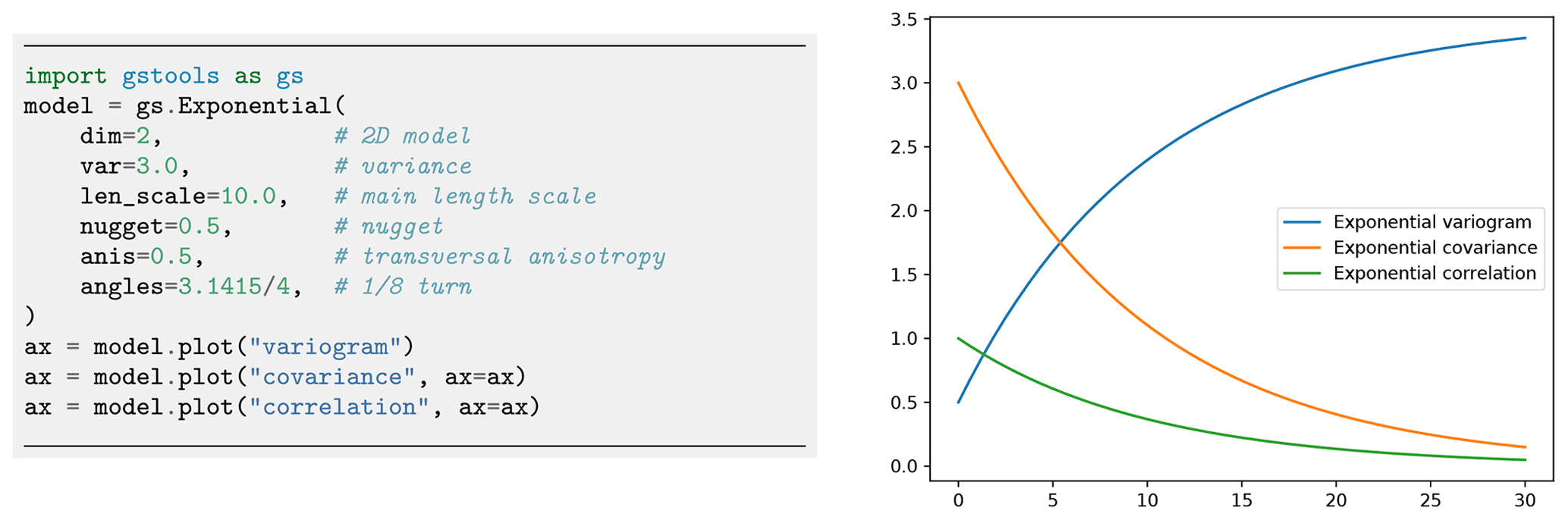
Every covariance model is defined by at least six parameters: dimension dim, variance var, main length scale len_scale, rescale factor rescale, anisotropy ratios anis and rotation angles angles, with the last two being dimension dependent.
Figure 1 shows an example code for instantiating an exponential model and the resulting model functions exemplifying the parameters. Table 1 provides an overview of the predefined models in GSTools.
Table 1Predefined covariance models in GSTools.
Formulas including the subscript (h<1) are piecewise-defined functions being constantly zero for h≥1. Here, h is the non-dimensional distance, d is the dimension, Γ(x) is the gamma function, Kν(x) is the modified Bessel function of the second kind, Jν(x) is the Bessel function of the first kind, is the ordinary hyper-geometric function and Eν(x) is the exponential integral function (Abramowitz et al., 1972). All other variables are shape parameters of the respective models.
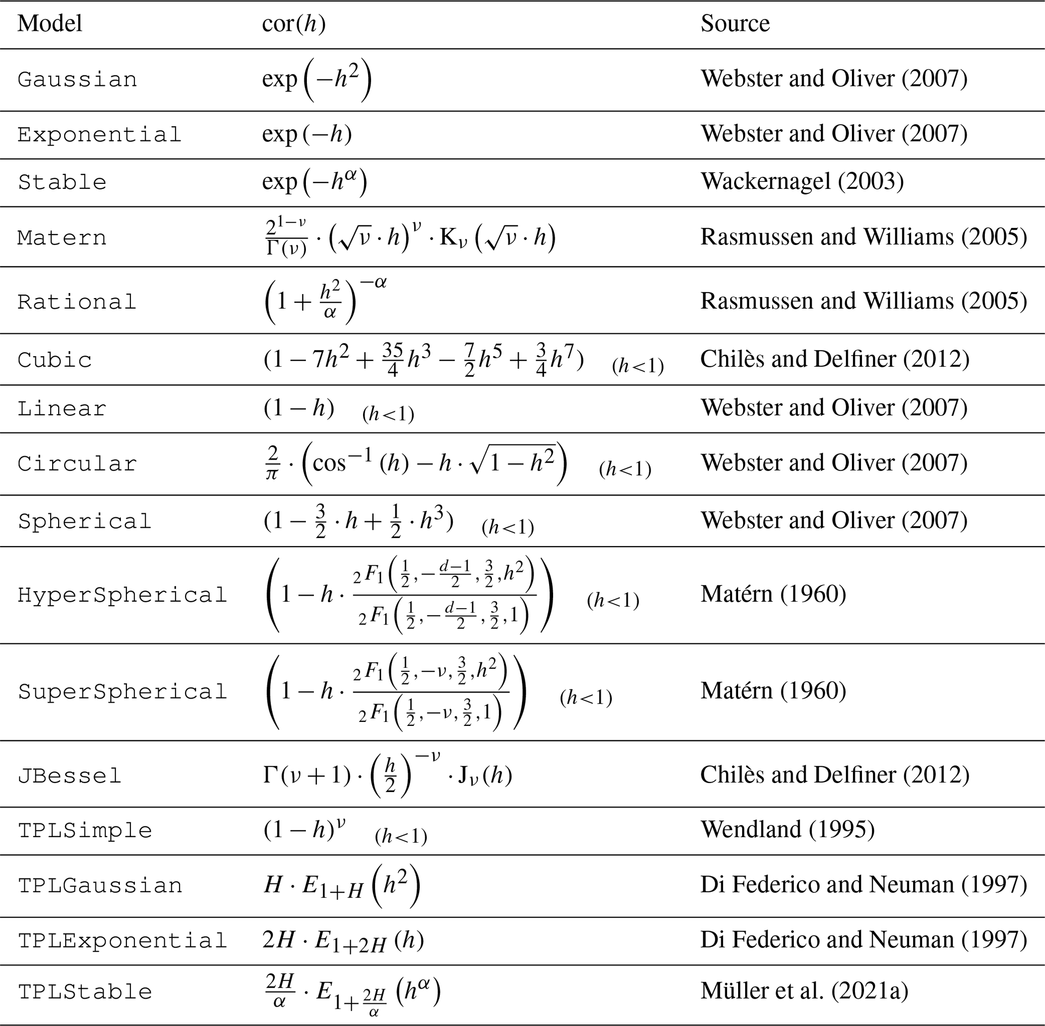
In addition to the predefined covariance models, users can specify their own model functions by providing a normalized correlation function. Figure 2 shows a reimplementation of the exponential model in only three lines of code.
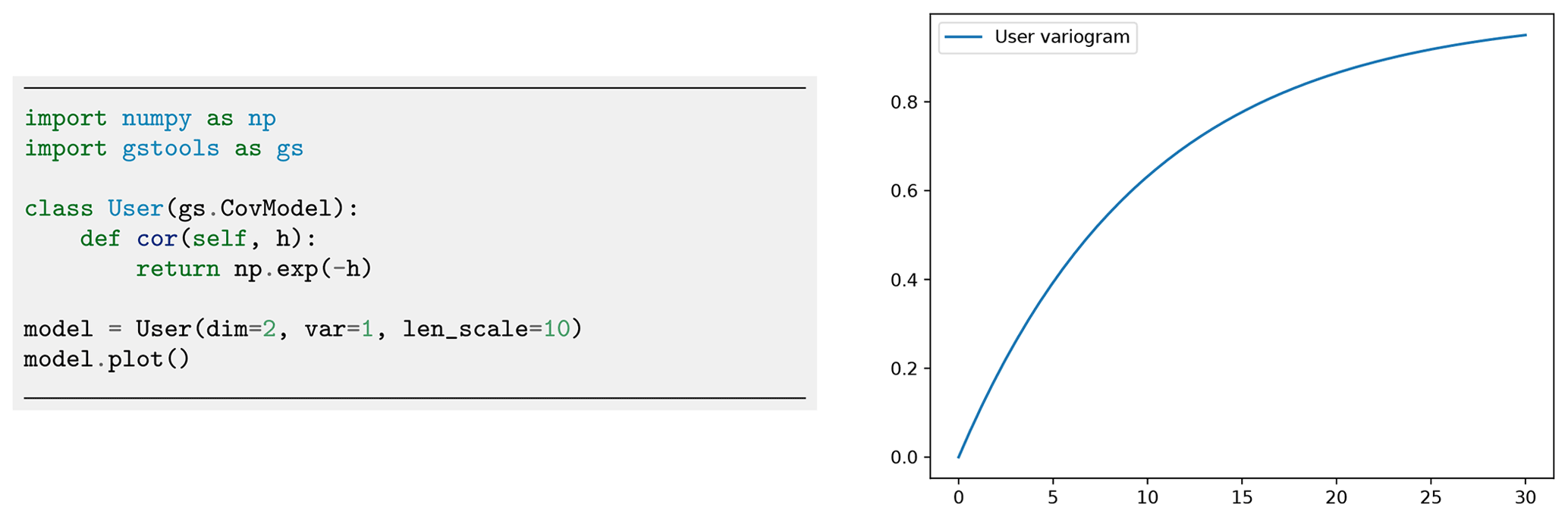
Figure 2Initialization of a user-defined exponential covariance model. The only thing that needs to be defined is the normalized correlation function cor.
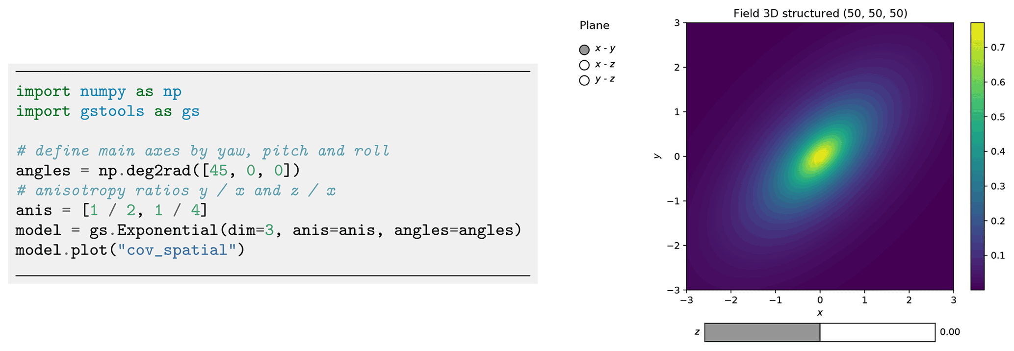
Figure 3Spatial covariance structure of an anisotropic exponential model in 3D plotted with the built-in interactive routines of GSTools.
The example shows an eighth turn on the xy plane with anisotropy factors . Rotation angles are given in radians.
The dimension-dependent spectrum of an isotropic covariance model can be called with model.spectrum. It is directly calculated from the covariance function by the following:
Here, and are the norms of the corresponding vectors, and ℋ is the Hankel transform, which provides a mathematically self-contained and numerically robust formulation of the radially symmetric Fourier transformation.
GSTools makes use of an implementation of ℋ provided by the Python package hankel (Murray and Poulin, 2019; Ogata, 2005).
For models with a known analytical solution, GSTools uses them for improved computations.
A prerequisite for kriging or random field generation is that the applied covariance function is positive (semi-)definite. That can be checked through the spectral density which is derived by the following (note that S only depends on the norm of k):
From Bochner's theorem (Rudin, 1990), it follows that the spectral density is a probability density function if and only if the underlying covariance function is positive (semi-)definite, which all predefined models in GSTools satisfy.
As a consequence, the error variance during kriging is always non-negative.
2.1.2 Anisotropy and rotation
Variograms are typically defined based on the lag distance r, resulting in an isotropic model.
However, many natural processes involve anisotropy with varying correlation ranges in different (orthogonal) directions.
An example is hydraulic conductivity, where anisotropy typically arises from the geologic stratification.
The implementation of anisotropy in GSTools is based on the non-dimensional distance (Rubin, 2003):
where is the main length scale incorporating the rescale factor s, represents the anisotropy ratios and represents the distances along the main axis of correlation resulting in the isotropic distance .
Consequently, GSTools uses a main length scale, a set of anisotropy ratios and a set of rotation angles to fully describe an anisotropic model.
In practice, the main directions of correlation do not necessarily follow the principal axis. The CovModel accounts for rotation through rotation angles, where their number m depends on the dimension d: .
In two dimensions, rotation is fully described by a single angle for rotation in the xy plane, and in three dimensions three angles are applied to the xy plane, xz plane and yz plane, respectively. In three dimensions these are often referred to as Tait–Bryan angles yaw, pitch and roll (Goldstein, 1980); see Fig. 3 for an example.
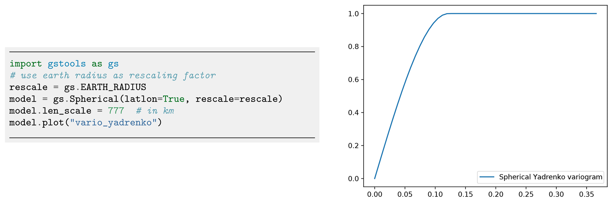
Figure 4Initialization of a Yadrenko covariance model. We use the Earth's radius as the rescaling factor to have a meaningful length scale. The routine vario_yadrenko still depends on the central angle given in radians.
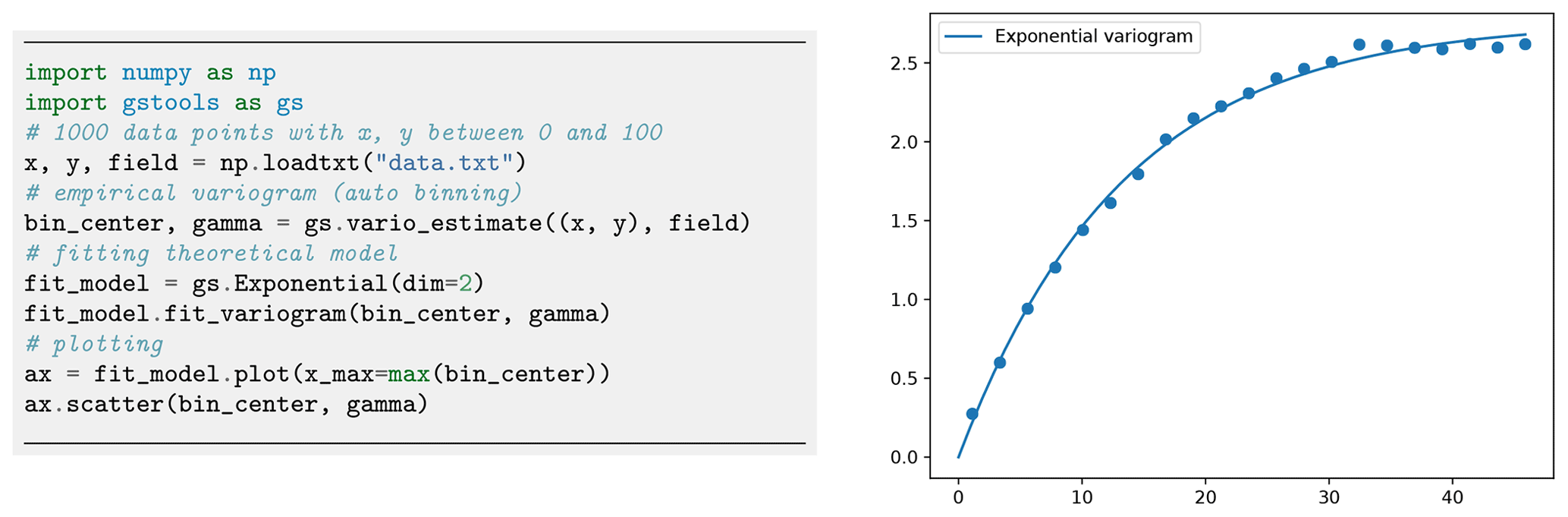
Figure 5Estimating an empirical variogram of synthetic unstructured data and fitting an exponential model. The number of bins was calculated to be 21 with a maximum bin distance of ca. 45.
One unique feature of GSTools is the support of arbitrary dimensionality in all provided routines.
For rotation in higher dimensions, we apply the following scheme: the first angles coincide with those of the next lower dimension, and the added d−1 angles describe rotations in the planes of the added dimension (in 3D: xz and yz).
Thus, there are 6 rotation angles in 4D, 10 in 5D, etc. Rotation in higher dimensions is only relevant for spatio-temporal modelling with three spatial dimensions and application to other fields of research with high-dimension data.
The scheme was chosen for metric spatio-temporal models to account for spatial anisotropy in a similar way as a simple spatial model.
Rotation in the xixj plane is described by the matrix .
The order of rotating planes is determined by the described scheme, i.e. (xy plane), , (xz plane) (yz plane), etc. These values define a rotation matrix Rot to transform principal axes to the directions of correlation and the back-rotation matrix for the inverse:
The alternating signs of the rotation angles were chosen to match Tait–Bryan angles in 3D.
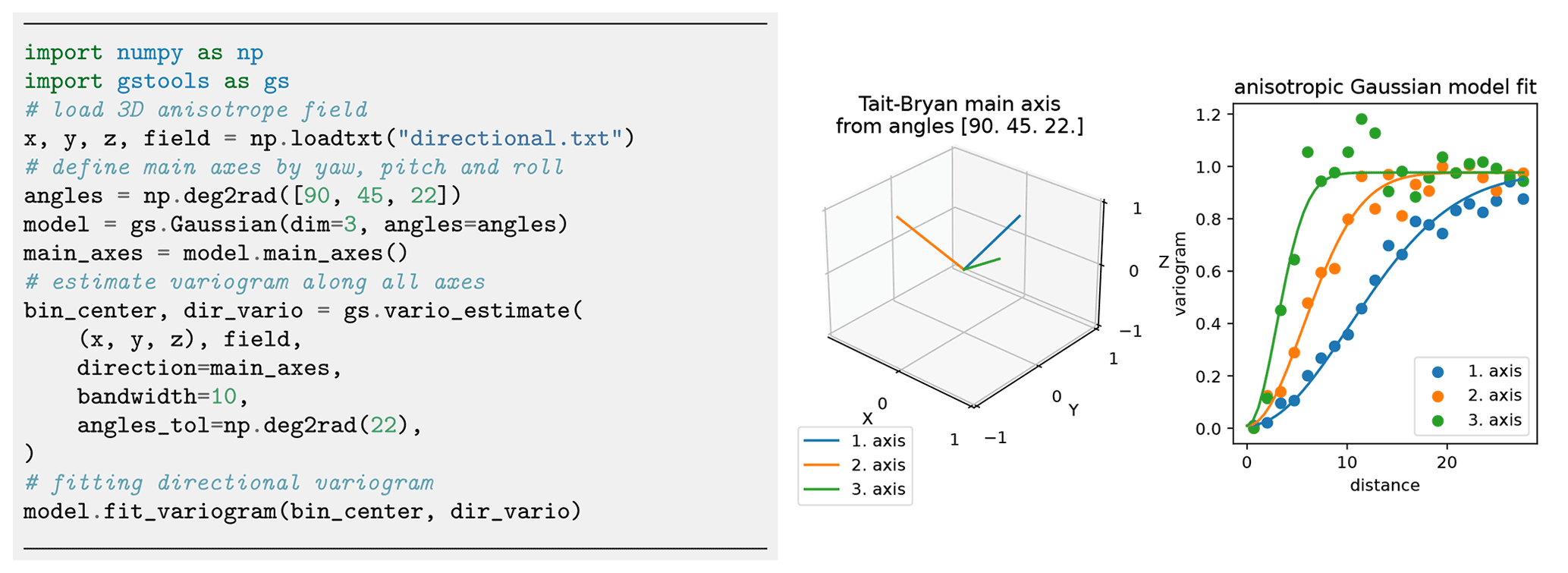
Figure 6Estimation of directional variograms for given main axes: the code snippet shows the setup for estimating and fitting the variogram to an anisotropic field. The graphs show the main axes of the rotated model and the fitting results. Plotting commands have been omitted.
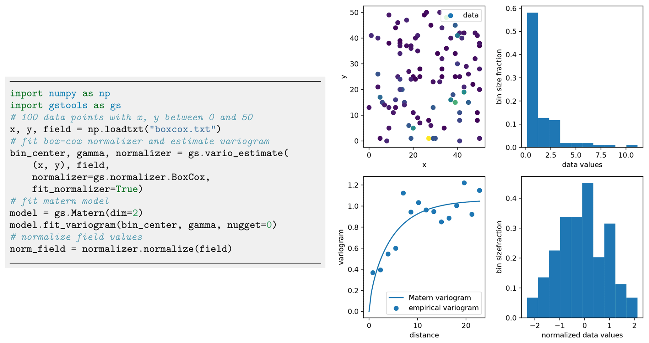
Figure 7Estimating an empirical variogram (bottom left) of synthetic unstructured data (top left) after Box–Cox normalization of skewed input values. Panels on the right show the histogram of the data values before (top) and after (bottom) the normalization. For demonstration purposes, a Matern model was fitted to the empirical variogram. Plotting commands have been omitted.
For applying or removing anisotropy, we define the isotropify matrix and anisotropify matrix . Combining these two types of matrices allows us to isometrize (i.e. isotropify and derotate) and anisometrize (i.e. rotate and anisotropify) spatial points via the following:
GSTools provides the routine CovModel.isometrize to convert spatial positions to their derotated and isotropic counterparts as required by Eq. (6) and the routine CovModel.anisometrize to invert this:
2.1.3 Geographical coordinates
Earth's surface is a non-Euclidean manifold, and all large-scale, geographically referenced data will necessarily reflect that. We deal with the non-Euclidean nature of this kind of data by assuming the Earth to be a perfect sphere and then using the fact that the distance between two points and is given by their latitude (ϕ) and longitude (λ) and can be described by a central angle calculated from the great circle distance:
A huge family of valid models on the sphere can be derived from 3D models by inserting the chordal distance which results in the associated Yadrenko covariance model CY (Lantuéjoul et al., 2019):
The underlying manifold introduces new restrictions for covariance models to be positive definite. The manifold structure of the sphere only allows for isotropic models. For small-scale applications, it is valid to assume anisotropy. An appropriate adaption is the use of a 2D projection like Gauss–Krüger coordinates. We provide Yadrenko models as a unified representation for non-Euclidian coordinates since they facilitate all presented models to be used with geographical coordinates as demonstrated in Fig. 4.
2.1.4 Empirical variogram, data preparation and model fitting
The empirical variogram is an important tool for analysing spatially correlated data. It is estimated with the subpackage gstools.variogram, which provides two estimators for the empirical variogram: Matheron and Cressie (Webster and Oliver, 2007).
The default Matheron's estimator for a variogram γ of a spatial random field U is given by
where M(r) is the set of all pairwise spatial random field points, separated by the distance r and a certain tolerance ε>0.
Cressie's estimator, which is more robust to outliers, is given by
Both estimators require predefined bins M(r) to group the pairwise point distances of the given field. GSTools provides a standard binning routine, where the maximal bin width is set to one-third of the diameter of the containing box of the field, the number of bins is determined by Sturges' rule (Sturges, 1926) and all bins have equal width.
Figure 5 provides an example of the variogram estimation of an unstructured spatial random field with automatic binning.
GSTools accounts for anisotropy by providing estimating routines for directional variograms along a specified direction with a certain angle tolerance and bandwidth. When providing orthogonal axes, it is possible to fit a theoretical model and its anisotropy ratios as shown in Fig. 6.
Determining the main rotation axes from given data, however, is up to the user and beyond the scope of the presented GSTools version.
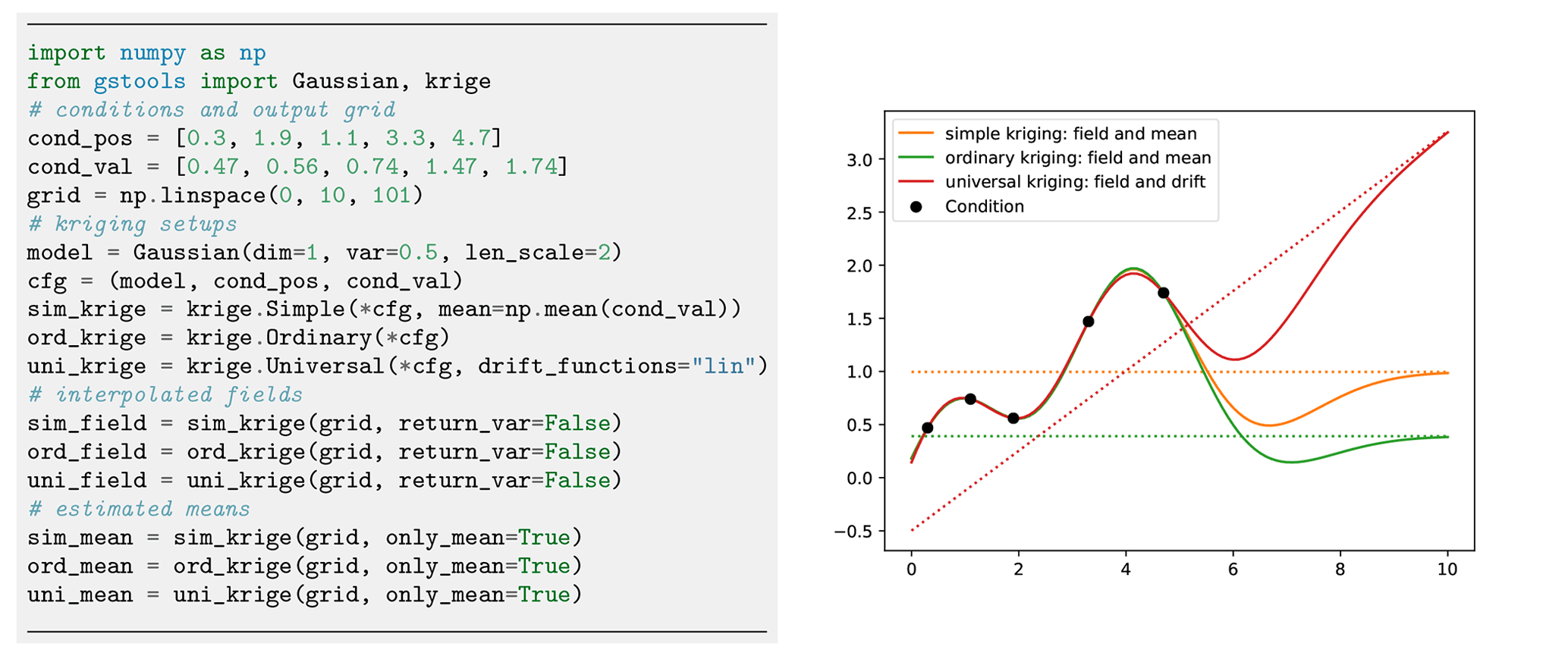
Figure 9Comparison of simple, ordinary and universal kriging. All three routines have a similar setup, where simple kriging needs an estimated mean and where universal kriging needs additional drift functions. Plotting commands have been omitted.
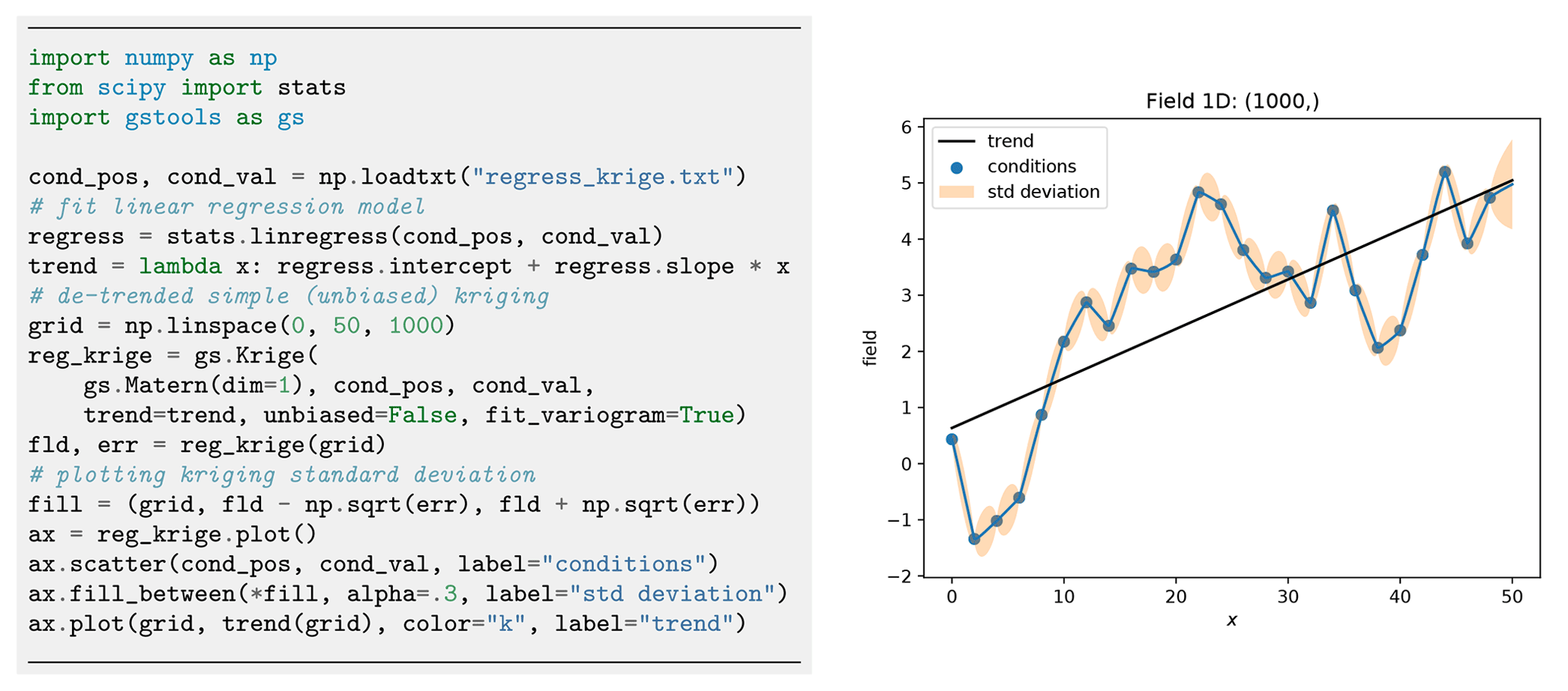
Figure 10A simple setup for linear regression kriging. Although the interpolation coincides with a piecewise linear function, we gain information about the error variances between the conditioning points as shown in the right plot.
Field data often do not follow a normal distribution, which is a crucial assumption for variogram estimation.
For example, transmissivity is usually assumed to be log-normally distributed (Dagan, 1989), while rainfall data are normalized by applying the Box–Cox transformation (Cecinati et al., 2017).
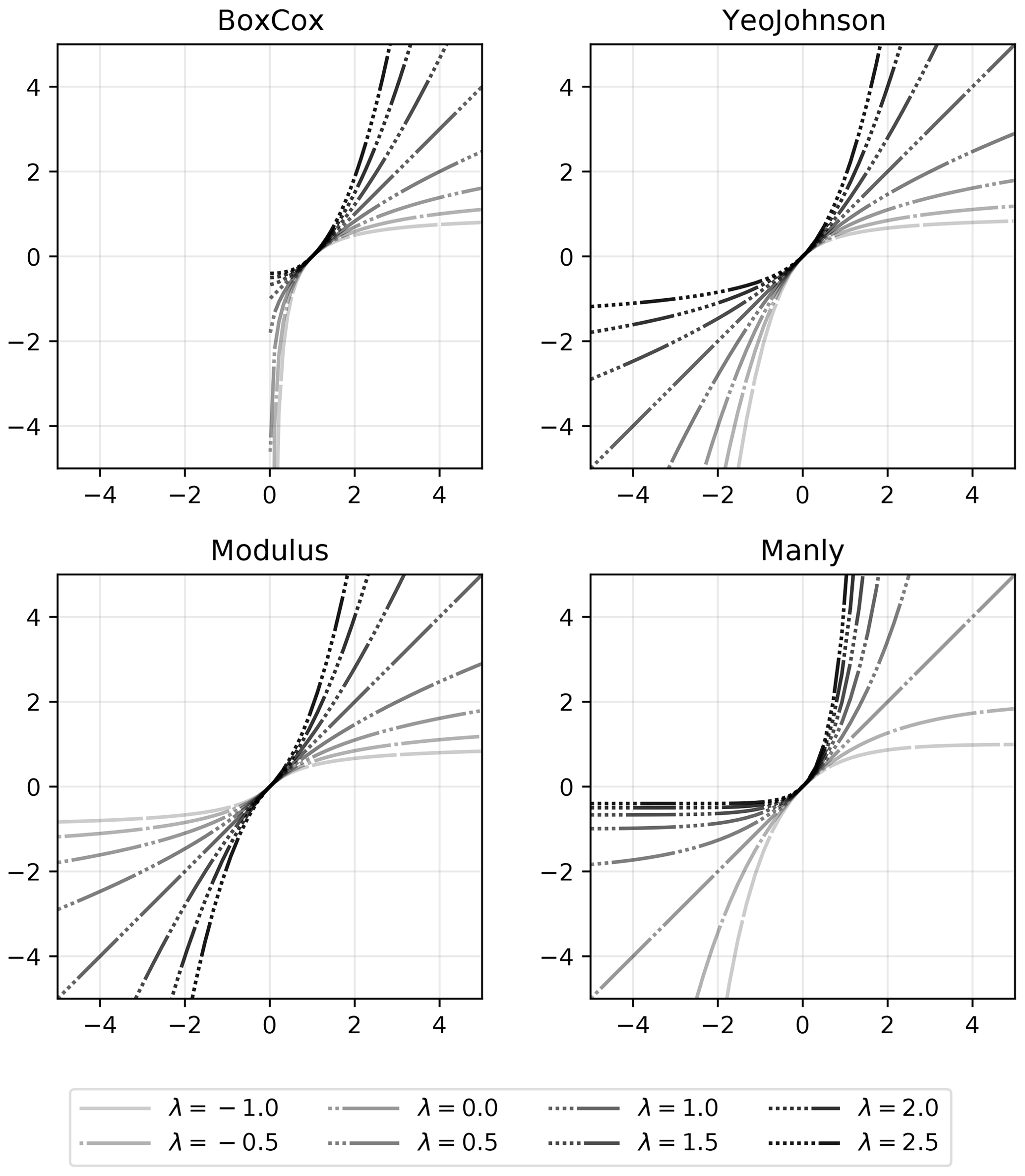
GSTools provides a set of normalizers based on power transforms, which can be fitted to a given data set using a maximum likelihood approach (Eliason, 1993): LogNormal, BoxCox (Box and Cox, 1964), YeoJohnson (Yeo and Johnson, 2000), Modulus (John and Draper, 1980) and Manly (Manly, 1976).
An example application is shown in Fig. 7, and a comparison of all provided normalizers can be seen in Fig. 8.
GSTools also provides routines to detrend data. For example, temperature could decrease with elevation or conductivity could decrease with depth.
Another application is analysing spatial correlation of residuals after application of a regression model to the data. All routines dealing with data have the keywords trend, normalizer and mean, where the last keyword describes the mean of the normalized data.
2.2 Kriging, random fields and conditioned random fields
2.2.1 Kriging
The subpackage gstools.krige provides routines for Gaussian process regression, also known as kriging, which is a method of data interpolation based on predefined covariance models (Wackernagel, 2003).
Kriging aims to derive the value of a field z at some point x0, when there are fixed conditioning values z(x1)…z(xn) at given points x1…xn.
The resulting value z0 at x0 is calculated as a weighted mean , where the weights, , are determined by the specific kriging routine.
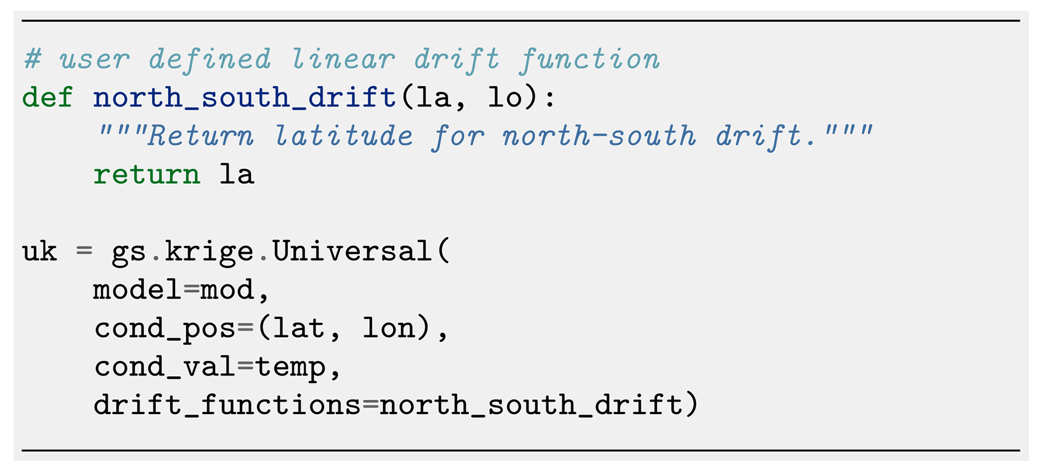
We provide multiple kriging routines derived from the Krige class. (i) Simple: the data are interpolated with a given mean value for the kriging field. (ii) Ordinary: the mean of the resulting field is unknown and estimated alongside the interpolation (unbiasedness). (iii) Universal: in addition to ordinary kriging, one can provide drift functions . (iv) ExtDrift: like universal kriging but the drift is provided by an external source.
The advantage of using the general Krige class is the combination of all described features, such as for instance using universal kriging with a functional drift together with additional external drifts.
A typical scenario is a temperature interpolation with an assumed north–south drift (functional drift) and a linear correlation to altitude (external drift).
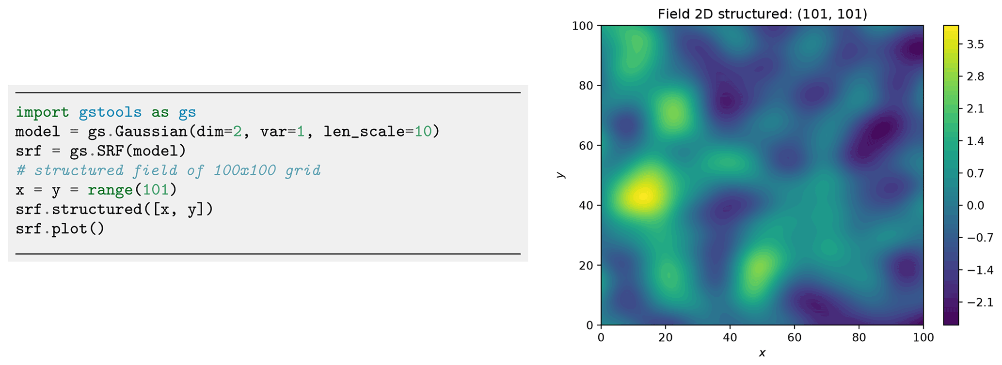
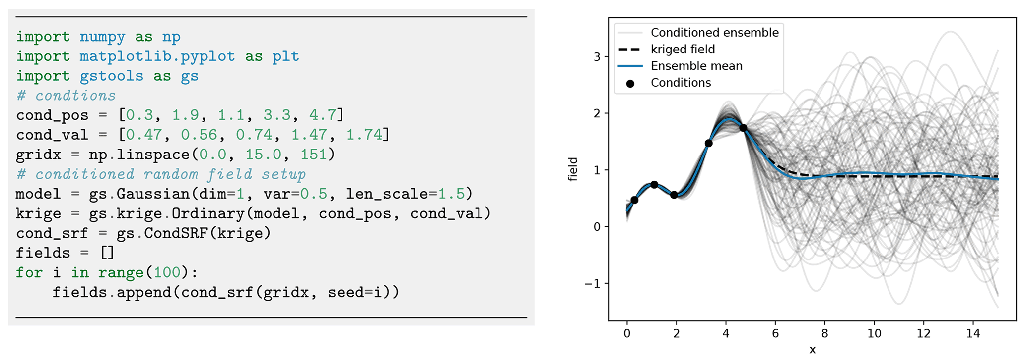
Figure 12An example for an ensemble of 1D random fields conditioned to five measurements (dots). Plotting commands have been omitted.
Since all variogram models in GSTools assume weak stationarity, the kriging system is always built on the associated covariance function:
with being the covariance matrix, depending on the conditioning points and the given model. is the covariance vector for the target point x0. is a submatrix containing the functional drift values at the conditioning points and at the target point, where k is the number of functional drifts. is a submatrix containing the external drift values at the conditioning points and at the target point, where l is the number of external drifts. The parameters μ, and are Lagrange multipliers for the unbiased condition, the functional drifts and the external drifts, respectively. The vector 1 and its Lagrange multiplier μ are given in brackets since their appearance depends on whether the system should be unbiased or not (ordinary vs. simple kriging). Note that the number of functional drifts k and external drifts l can be zero, depending on whether they are given or not.
GSTools also provides the possibility to incorporate measurement errors variances for each conditioning point by adjusting the covariance matrix (Wackernagel, 2003):
By default, the measurement error variances, , are set to the model nugget. In order to get numerically stable results, we solve the kriging system with the pseudo-inverse matrix, which has the advantage that redundant data or multiple measurements at the same location are averaged out in the resulting field (Mohammadi et al., 2017).
One last feature is the capability of kriging the mean (Wackernagel, 2003), which allows for deriving the mean value estimated during ordinary kriging or estimating the mean drift determined from given functional and/or external drift terms as shown in Fig. 9. A minimal example for regression kriging is shown in Fig. 10.
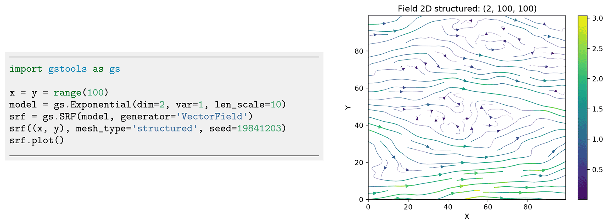
Figure 13Generation of a structured incompressible random vector field with exponential variogram.
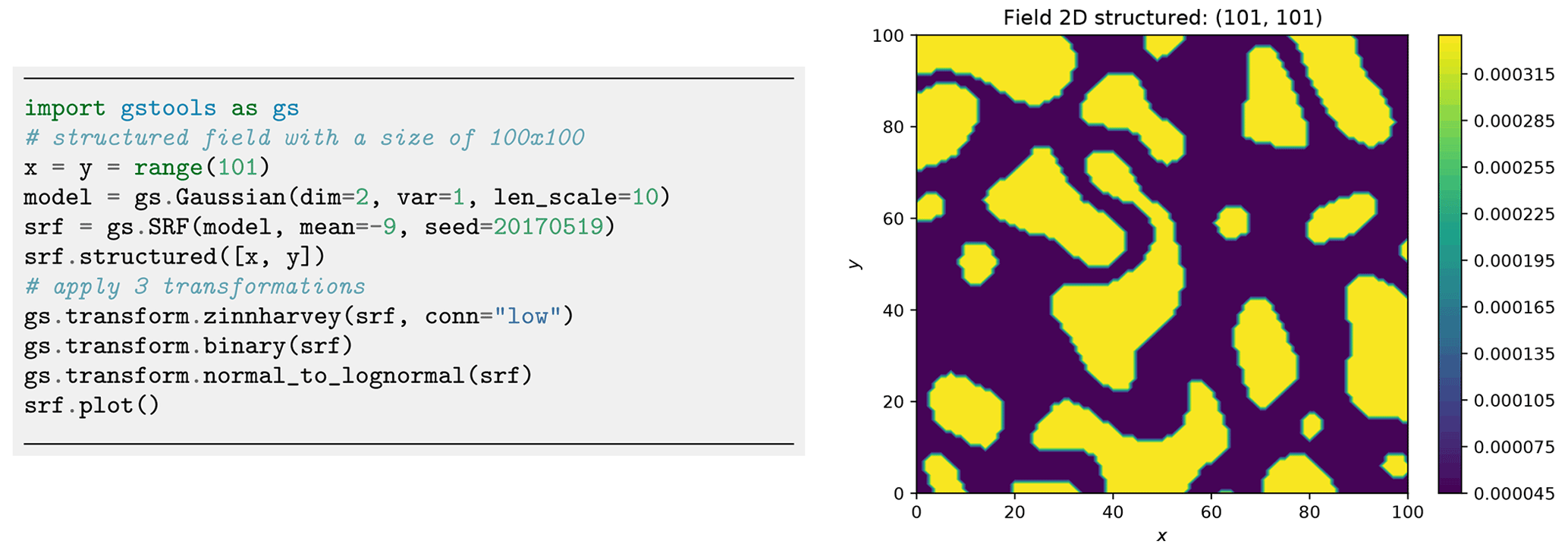
Figure 14Example of a log-transformed binary field with the low values being connected by applying the zinnharvey, binary and lognormal transformations successively.
2.2.2 Random fields
A core element of GSTools is the spatial random field generator class SRF.
A covariance model (Sect. 2.1) is needed to instantiate a spatial random field.
We provide two ways for field generation: structured or unstructured.
In both cases, the positions at which the field will be evaluated are given by a pos argument.
In the structured case, pos contains one tuple per dimension, each defining the subdivision of the corresponding axis resulting in a rectilinear grid.
For unstructured grids, the pos tuple contains the x, y and z coordinates of every evaluation point.
SRF allows for controlling the underlying pseudo-random number generation by a seed to reproduce field generation. A code example is given in Fig. 11.
Field generation is performed through the randomization method (Kraichnan, 1970; Heße et al., 2014), which utilizes the spectral density (Eq. 5) of the variogram model to approximate a Wiener process in Fourier space by
where N is the number of Fourier modes of the approximation. The random variables are mutually independent and are drawn from a standard normal distribution. The ki values are mutually independent random samples, which are drawn from the spectral density with the aid of emcee, a Python package for Markov chain Monte Carlo sampling (Foreman-Mackey et al., 2013).
The randomization method is implemented in the RandMeth class and used by default.
The RandMeth routines create isotropic random fields. Thus, the corresponding covariance is radially symmetric, and the spectral density can be calculated by the Hankel transformation. Anisotropy is realized by rescaling and rotating the input points. The workflow allows users to generate a random field only from a given correlation, covariance or variogram function.
A key advantage of the randomization method implementation is the possibility to extend a generated SRF seamlessly, which not only preserves its statistical properties but also preserves the actual realization of the SRF. Potential applications are the following. (i) Particle simulations, where random incompressible velocity fields can be generated exactly at the location of the individual particles (see workflow in Sect. 2.3.1). It avoids interpolation errors, arising from grid-based velocity fields. (ii) If concentration plumes are simulated on a large domain, the SRF can be calculated on demand only for the time dependent spatial extent of the plume. And (iii) for high-performance computing applications, the field generation can be directly coupled to the domain decomposition, and each task only generates the SRF for its part of the domain. There are two main classes of alternative methods to the randomization method (Heße et al., 2014). By decomposing the covariance function, small spatial random fields can be computed very fast. But the computational cost quickly becomes unfeasible as the field grows in size. A second and quite popular class is the sequential Gaussian method, which can also create conditioned spatial random fields. However, numerical problems can arise if the underlying correlation function is smooth at the origin, and the computational costs also become unfeasible for highly resolved random fields (Emery, 2004).
Just like the kriging routines, the spatial random field generator allows for incorporating predefined trend, normalizer and mean for a greater variety of distributions.
A special SRF class feature is the capability to perform variance upscaling to respect generation of random fields on mesh cells with a certain volume. We hereby use the upscaling method coarse graining (Attinger, 2003) to rescale the variance in Eq. (19) at each target point based on a given filter volume size λ:
where ℓ is the correlation length, and is the filter size derived from the cell volume V depending on the field dimension, assuming the cell element is a hypercube. This approach was derived from the groundwater flow equation, assuming a Gaussian covariance model and should therefore be used with caution in differing scenarios. An example is provided in the workflow in Sect. 4.3.
2.2.3 Conditioned random fields
When point measurements of a target variable are available, they need to be considered when generating random fields. GSTools provides a class CondSRF combining kriging and random field generation, where we first derive the kriged field and the error variance and then generate a random field with zero mean where the variance in Eq. (19) is replaced with the estimated error variance.
This procedure is advantageous to classical sequential Gaussian simulation (Webster and Oliver, 2007), as (i) we make use of the randomization method to generate a single random field, and (ii) we only need to solve the kriging problem once and not sequentially.
Figure 12 shows an example of an ensemble of conditioned random fields in one dimension. Where measurements of the target variables are available, all realizations satisfy them. However, random fields behave as unconditional fields (i.e. of an ensemble with identical parameters, like mean, variance and correlation length) where no point measurements are available (x>6). Characteristics, such as the ensemble variance, significantly change given the distribution of measurements and conditioning. The ensemble mean and the kriging field coincide, proving that the kriging field is the best linear unbiased predictor for the given data.
2.3 Additional features
2.3.1 Incompressible random vector field generation
Kraichnan (1970) was the first to suggest a randomization method for studying the diffusion of single particles in a random incompressible velocity field. He came up with a randomization method which includes a projector, ensuring the incompressibility of the vector field.
When is the mean velocity (oriented towards the first basis vector e1), we generate random fluctuations with a given covariance model around . And at the same time, we ensure that the velocity field remains incompressible; that is, by using the randomization method (Eq. 19) and adding a projector p(ki) to every mode being summed:
Calculating verifies that the resulting field is indeed incompressible. An example is shown in Fig. 13. Things like boundary conditions cannot be modelled with this method, but it can be used, for example, in transport simulations of the saturated subsurface (Schüler et al., 2016) or for studying turbulent open water (Kraichnan, 1970).
2.3.2 Field transformations
GSTools generates Gaussian random fields while real data often do not follow a Gaussian distribution. This is typically addressed through data transformation.
GSTools provides a number of appropriate transformations beyond power transformations provided by the normalizer submodule (Sect. 2.1.4): (i) binary, (ii) discrete, (iii) boxcox (Box and Cox, 1964), (iv) zinnharvey (Zinn and Harvey, 2003), (v) normal_force_moments, (vi) normal_to_lognormal, (vii) normal_to_uniform, (viii) normal_to_arcsin and (ix) normal_to_uquad.
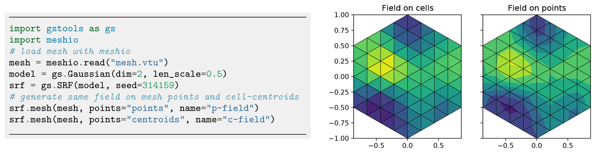
Figure 16Generating spatial random fields on finite element method (FEM) meshes: either on cell centroids (middle) or mesh points (right). Plotting commands have been omitted.
Transformations can be combined sequentially to create more complex scenarios as in Fig. 14. Note that, in contrast to normalizers, transformations cannot be fitted to given data, which leaves the choice of the best transformation to the user.
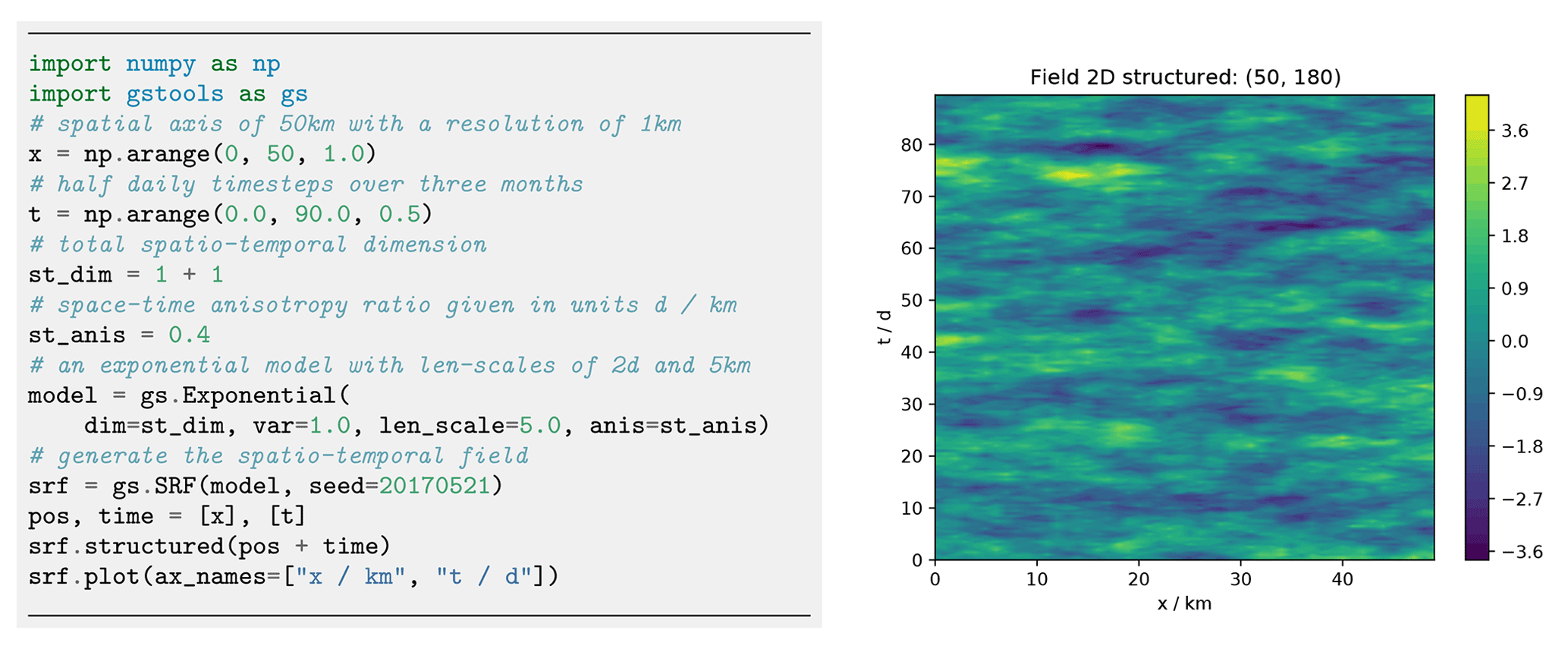
2.3.3 Spatio-temporal modelling
Spatio-temporal modelling provides insights into time-dependent stochastic processes like rainfall, air temperature or crop yield, which is of high practical relevance.
GSTools provides the metric spatio-temporal model (Cressie and Wikle, 2011) for all covariance models by enhancing the spatial with a time dimension, resulting in the spatio-temporal dimension dst:
where is the isotropified spatial distance as defined in Eq. (6), Δt is the temporal distance and the isotropified temporal distance.
The parameter κ accounts for a spatio-temporal anisotropy ratio and is the last entry of the anis array appended to the spatial anisotropy ratios.
The implementation in GSTools enables the direct incorporation of spatial anisotropy and rotation in a spatio-temporal model.
It further supports the use of arbitrary spatial dimensions in spatio-temporal models.
Figure 15 shows the generation of a spatio-temporal random field with one spatial dimension.
2.3.4 Working on meshes
For improved handling of spatial random fields as input for PDE solvers like the finite element method (FEM), GSTools provides an interface for a number of mesh standards, such as meshio (Schlömer et al., 2021), PyVista (Sullivan and Kaszynski, 2019) and ogs5py (Müller et al., 2020).
When using meshio or PyVista, the generated fields will be stored immediately in the mesh container.
There are two options to generate a field on a given mesh: either on the points (points="points") or on the cell centroids (points="centroids"), which is important depending on the specification of the variable in the numerical scheme. Figure 16 provides an example.
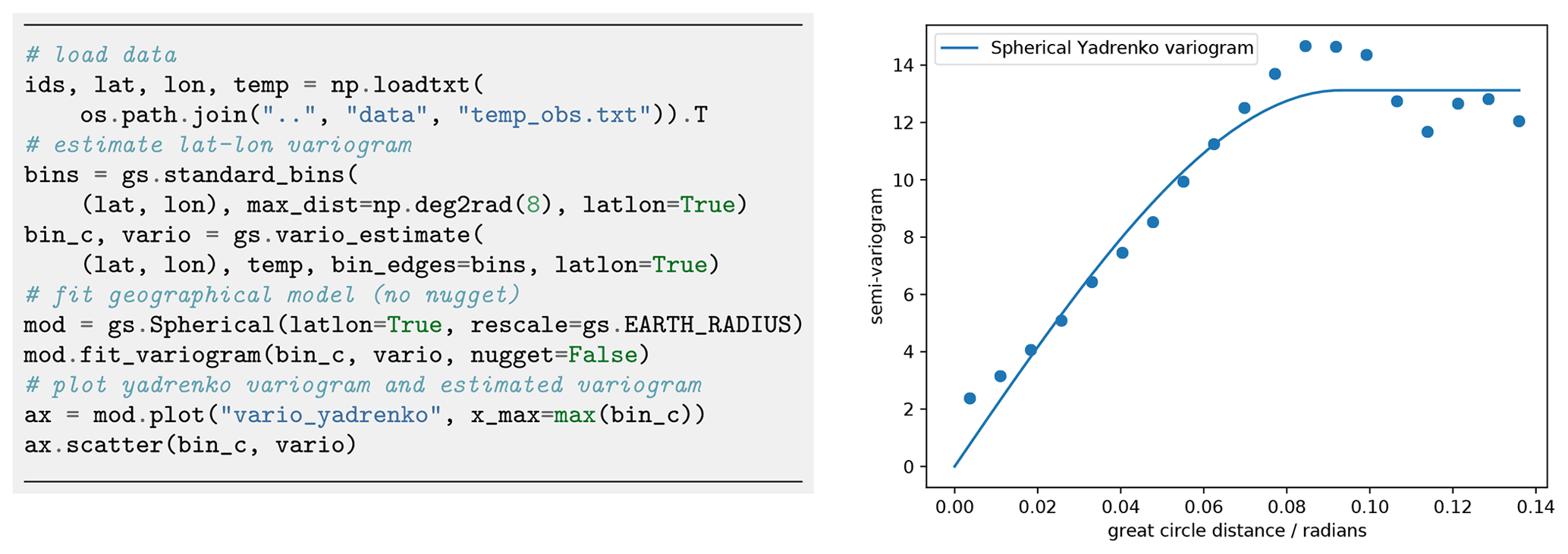
Figure 17Estimating the temperature variogram with geographic coordinates using the spherical Yadrenko model. Estimated length scale is ca. 0.9 (radians) and sill is around 13.
GSTools within the ecosystem of the GeoStat Framework GSTools is part of a larger suite of Python packages, collectively hosted on GitHub under https://github.com/GeoStat-Framework (last access: 31 March 2022).
The other packages in the GeoStat Framework complement some of the abilities of GSTools and form a comprehensive framework for geostatistical applications.
We introduce some packages and demonstrate how they interact with, enhance and leverage the abilities of GSTools.
3.1 ogs5py
ogs5py (Müller et al., 2020) provides a Python API for the FEM-based OpenGeoSys 5 (Kolditz et al., 2012) scientific software suite for hydrogeological processes like groundwater flow and transport modelling where data scarcity is a typical shortcoming.
Examples are point measurements of hydraulic head from observation wells and breakthrough curves from tracer experiments.
Inferring hydraulic conductivity from these data requires a modelling framework with integrated stochastic data generation.
The combination of GSTools with ogs5py enables a user to integrate the geostatistical modelling of an aquifer with hydrogeological simulations. Such an example for pumping test simulations is provided in Sect. 4.3.
3.2 welltestpy and AnaFlow
A pumping test is a cost-effective subsurface observation method typically used by hydrogeologists for aquifer characterization. The package welltestpy (Müller et al., 2021b) provides tools to handle, process, plot and analyse data from pumping test campaigns. It assists practitioners in identifying hydrogeological parameters by fitting measured drawdowns to some conceptual flow model. The package contains a number of examples that illustrate these abilities.
AnaFlow (Müller et al., 2021a) provides a wide range of analytical expressions for pumping tests under various conditions. Classical examples are Thiem's and Theis' solution assuming homogeneous aquifer properties. In addition, AnaFlow provides extended versions of both solutions, which account for aquifer heterogeneity and allow for estimating higher-order geostatistical parameters like variance and correlation length (Zech et al., 2012, 2016).
3.3 PyKrige
GSTools provides an interface to the stand-alone package PyKrige (Murphy et al., 2021) for more specialized kriging applications.
After 10 years of independent development, PyKrige has recently been migrated to the GeoStat Framework, and its functionality is currently integrated with the other packages.
So far, the covariance model can be exchanged between the packages.
In the future, PyKrige will become the kriging toolbox for the GeoStat Framework, providing advanced methods.
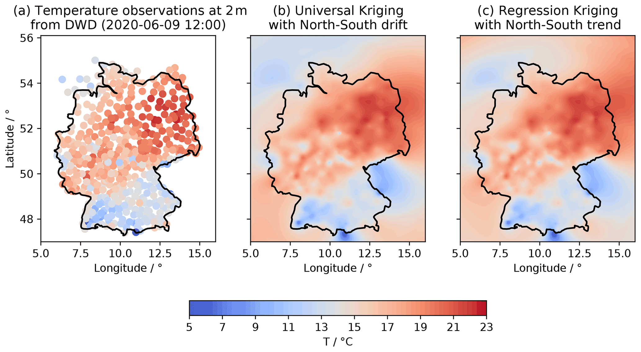
Figure 20Plot of temperature measurements (a), universal kriging interpolation (b) and regression kriging results (c).
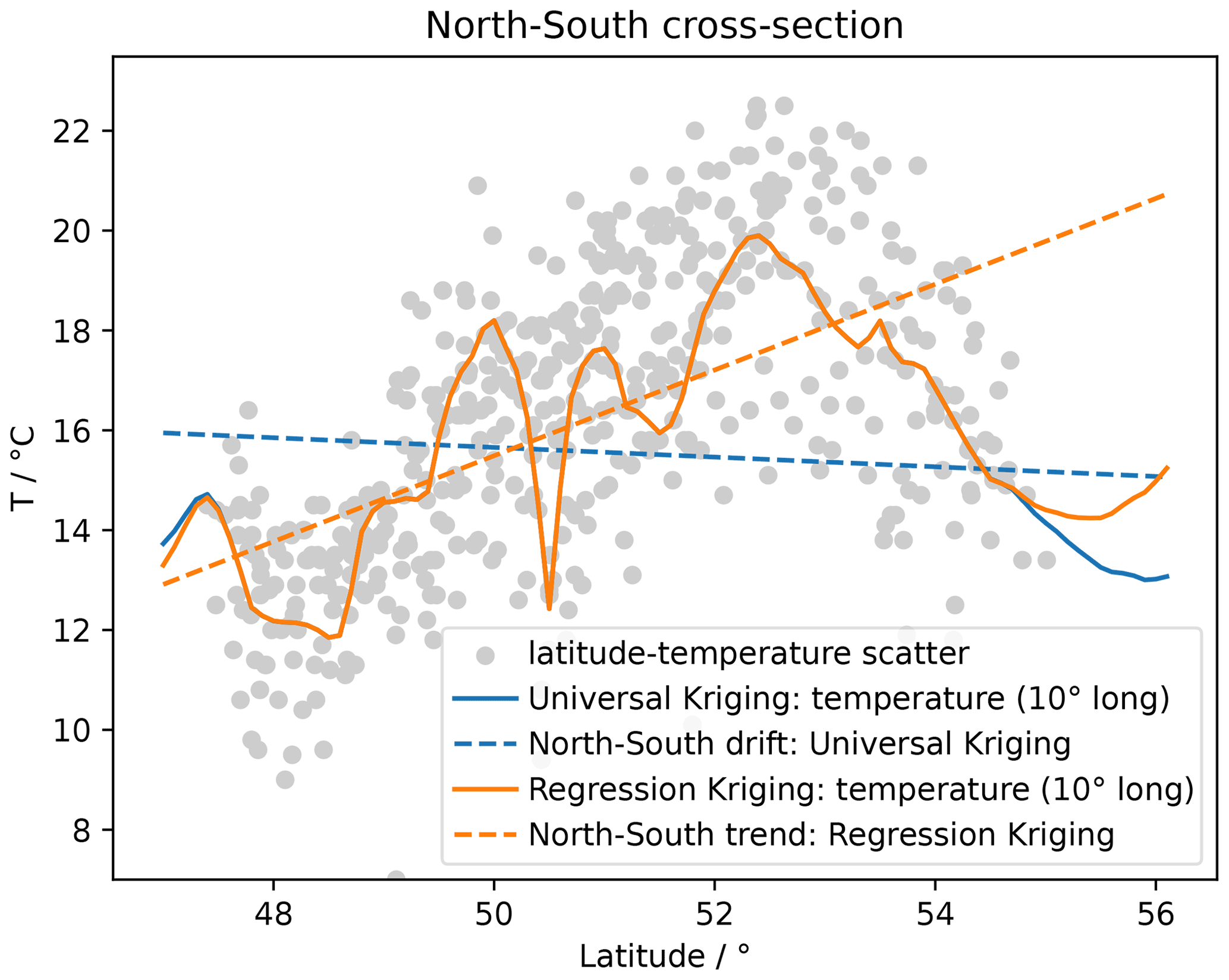
Figure 21Scatterplot of latitude–temperature values (grey dots), the linear regression result (dashed orange line), universal kriging mean drift (dashed blue line) and the cross-sections of the respective kriging interpolation (solid lines).
3.4 Development, documentation and installation
GSTools is compatible with Python versions ≥3.6, although previous releases support older versions of Python.
Performance-critical parts, like variogram estimation (Sect. 2.1.4), kriging summation (Sect. 2.2.1) and the summation of the randomization method (Sect. 2.2.2), are implemented in Cython (Behnel et al., 2011).
GSTools mainly depends on the SciPy ecosystem with its mandatory dependencies numpy (Harris et al., 2020) and scipy (Virtanen et al., 2020).
The source code is maintained under a GitHub organization for optimizing team efforts.
Users have the opportunity to communicate with developers by asking questions in a discussions forum, raising issues or improving code by making pull requests.
All packages come with detailed documentation via https://readthedocs.org (last access: 31 March 2022), which contains a range of tutorials explaining the features and a full API documentation created by Sphinx.
Continuous integration is established through GitHub actions where Python wheels are pre-built for the most common operating systems (Windows, Linux, MacOS) and Python versions to enable simple installation.
Each release on GitHub is directly deployed to the Python package index (https://www.pypi.org; last access: 31 March 2022) as well as conda-forge (conda-forge community, 2015).
An extensive set of unit tests are performed automatically and continuously through GitHub actions.
3.5 Interoperability
To integrate GSTools into the Scientific Python Stack, we provide a set of interfaces to other packages.
These include the above-mentioned packages ogs5py, meshio, PyVista and pyevtk (https://github.com/pyscience-projects/pyevtk, last access: 31 March 2022) for mesh operations.
Other packages for geostatistics are also supported, such as PyKrige (Sect. 3.3) and scikit-gstat (Mälicke, 2022), the latter having a focus on variography and can be used for more detailed variogram estimation.
For both packages, interfaces are provided to convert covariance models of GSTools to or from their counterparts in the respective package.
Another package worth mentioning is verde (Uieda, 2018), a Python library for processing and gridding spatial data.
Some of the features provided there can be easily combined with capabilities of GSTools such as detrending data to preprocess inputs.
Having explained the core features of GSTools, we now provide a couple of example applications covering the topic of kriging, variogram estimation, random field generation and coupling with other tools to achieve more elaborate workflows. The examples illustrate the abilities of GSTools and serve as a starting point for a user's project development.
All shown code snippets are taken from the actual workflow scripts and are not self-contained.
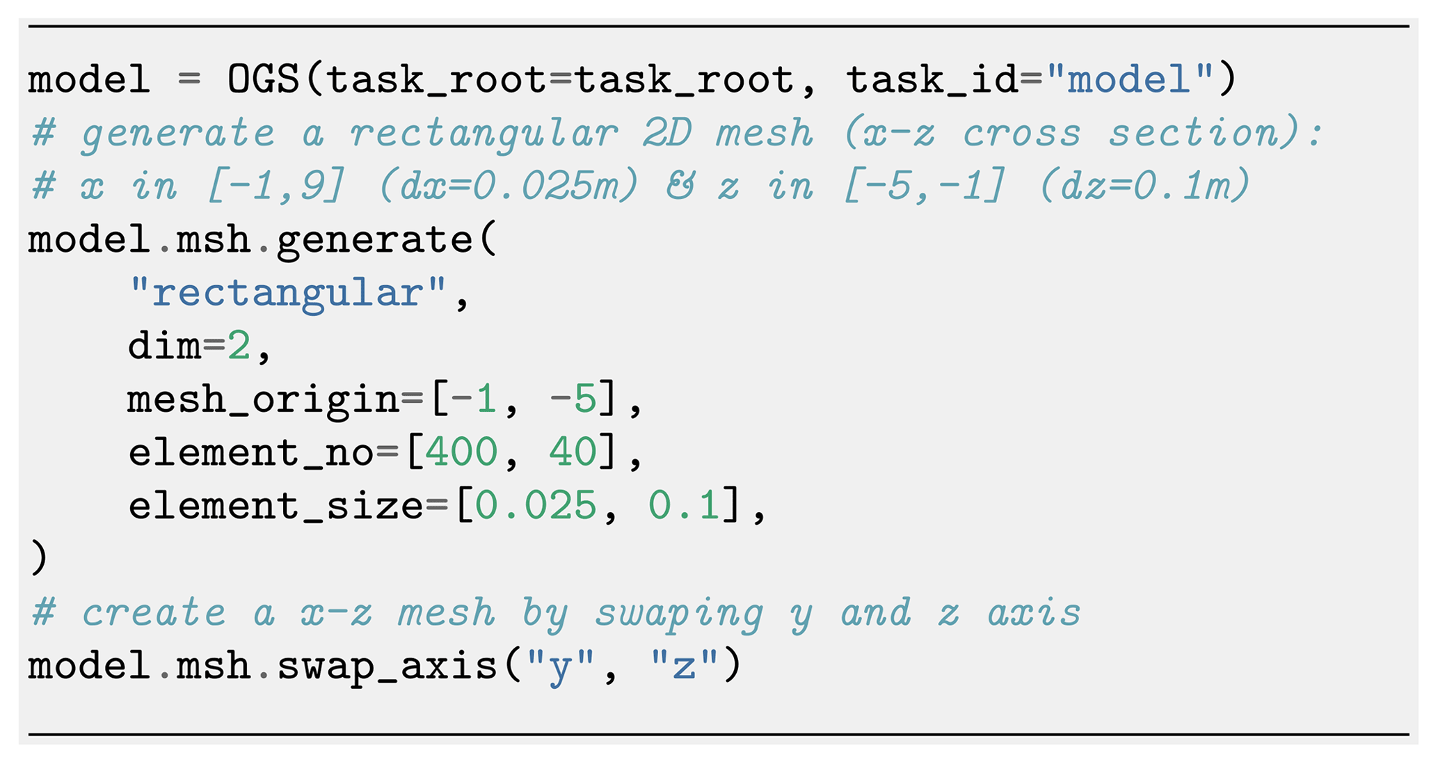
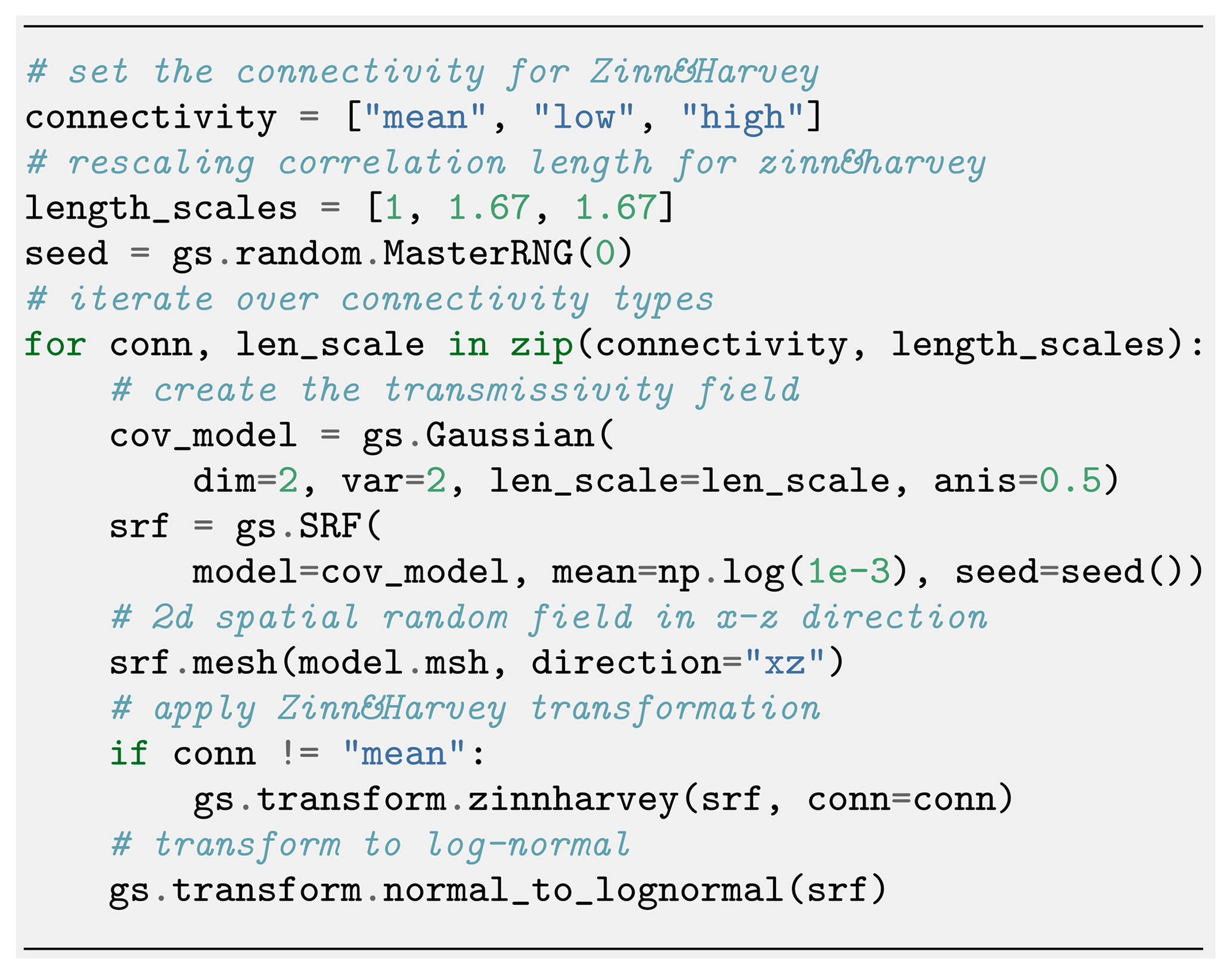
Figure 23Generating correlated log-normal SRFs adapted to the mesh settings of the numerical model for three connectivity structures following the Zinn and Harvey (2003) transformation.
4.1 Regression kriging vs. universal kriging: finding a north–south temperature trend
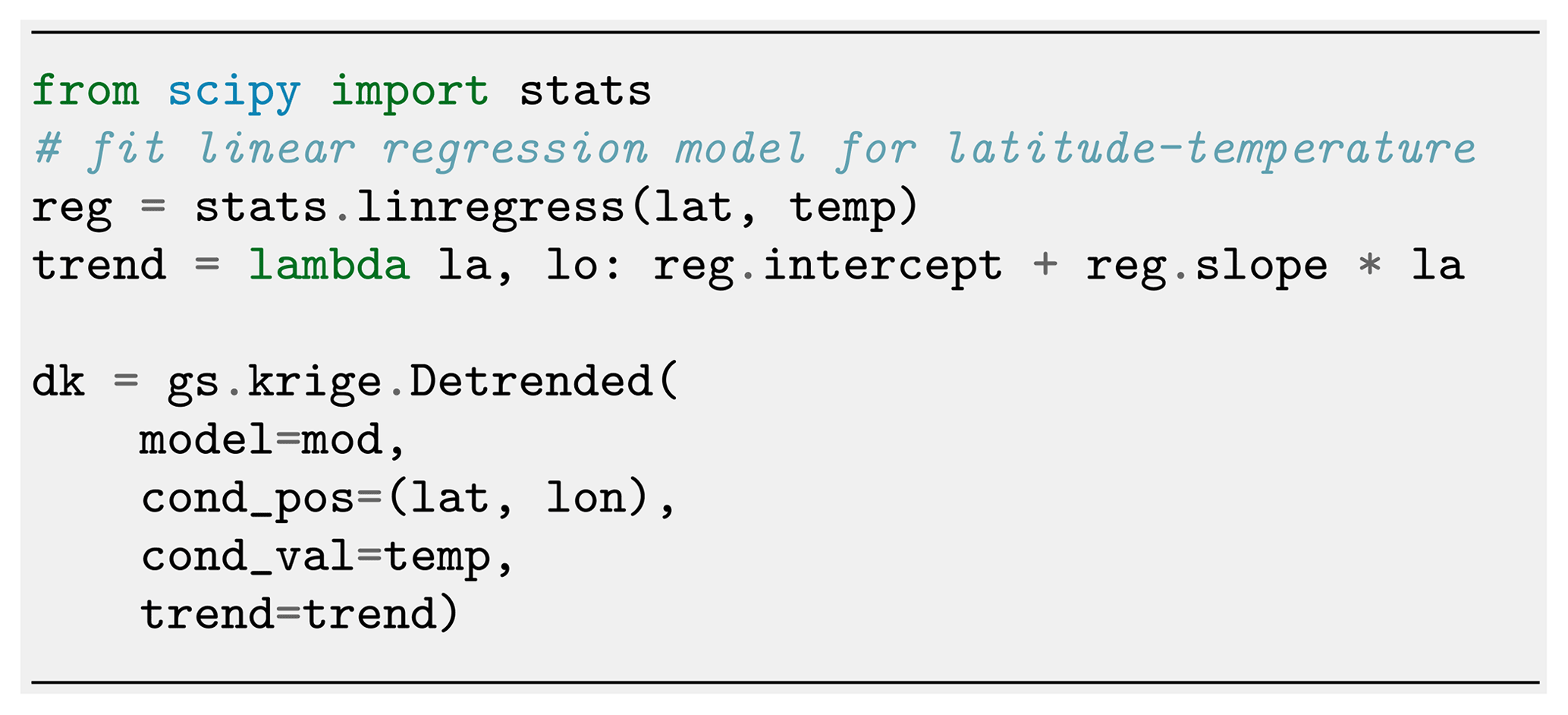
Kriging is a well-established interpolation method applied in many fields of natural science. We compare two options of incorporating auxiliary variables to calculate the kriging weights: (i) regression kriging (RK), where the trend of input data is estimated by regression and simple kriging is applied to the residuals, and (ii) universal kriging (UK), where the trend model is used as the internal drift in the kriging system. The methods differ in use of the covariance model. The linear RK does not incorporate spatial correlation information, while UK does through the drift function for calculating the kriging weights. Both methods are often considered to provide mathematically equal results, but we show that there are sensitive differences. The resources for this workflow are provided in Müller (2021).
As a data basis, we use measured temperature of the German weather service retrieved with the Python package wetterdienst (Gutzmann et al., 2021), which we examine for a linear north–south trend.
We use the established spherical covariance model in its Yadrenko variant suitable for geographical coordinates. Variogram estimation and fitting results are shown in Fig. 17.
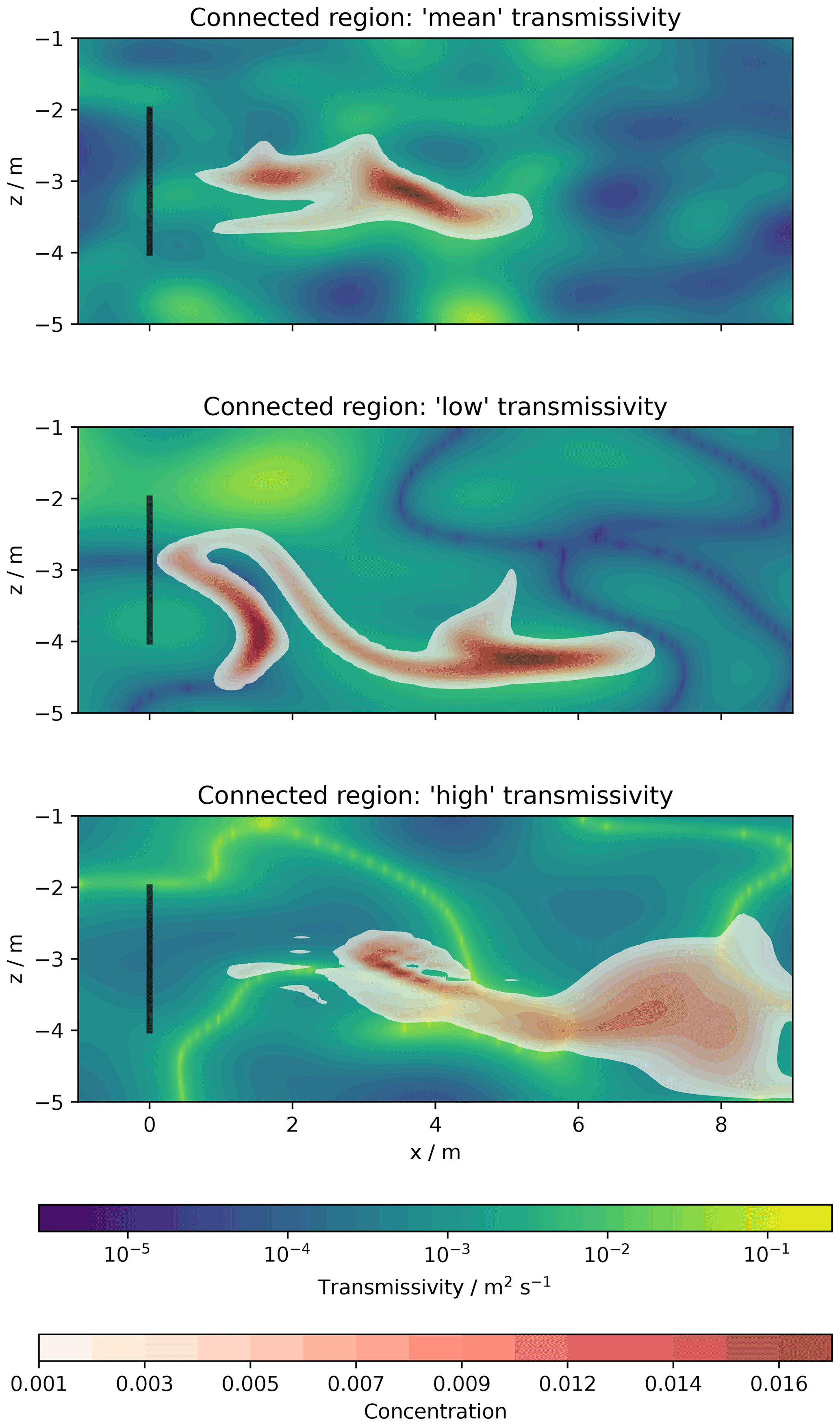
Figure 24Tracer transport simulation results: spatially distributed concentration plumes after 15 d with transmissivity distributions in the background.
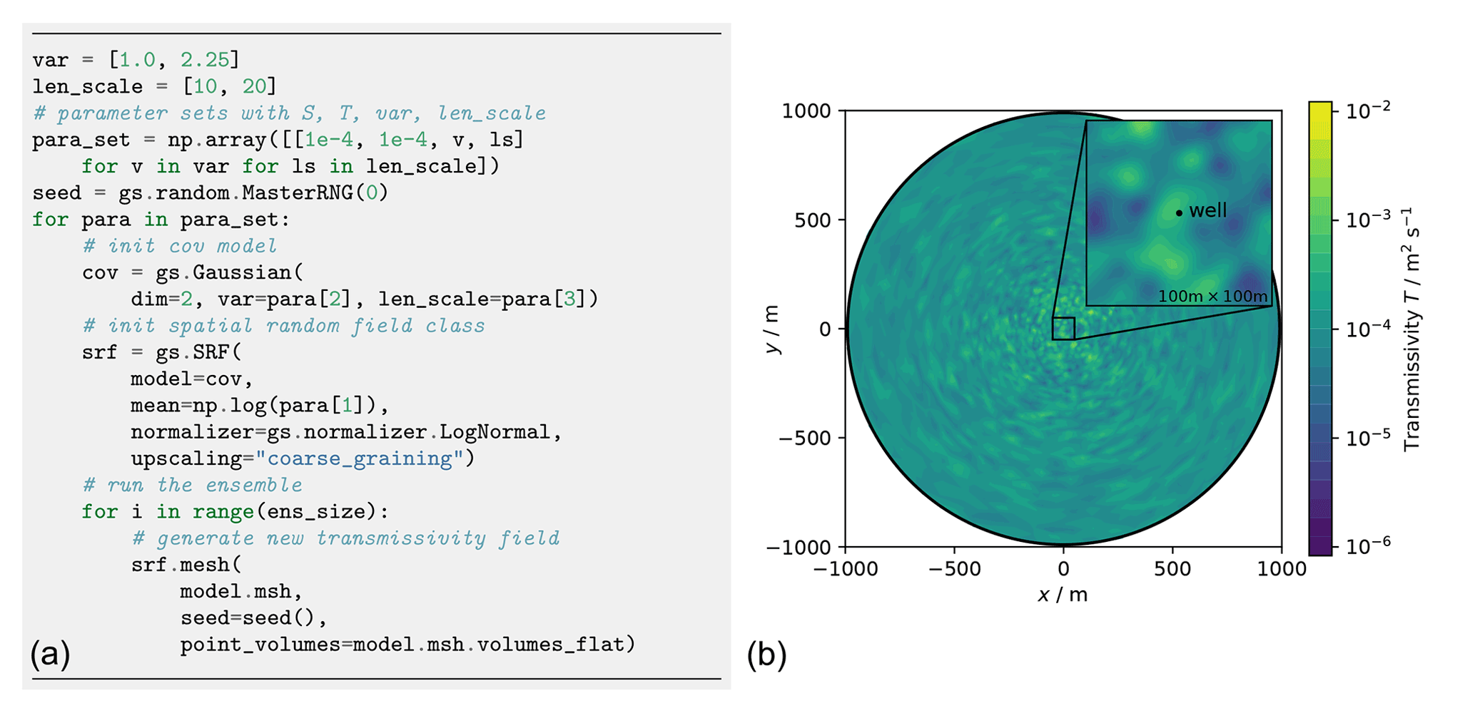
Figure 25Workflow to generate an ensemble of transmissivity fields on a given mesh (a). A single realization in shown in the right plot (b).
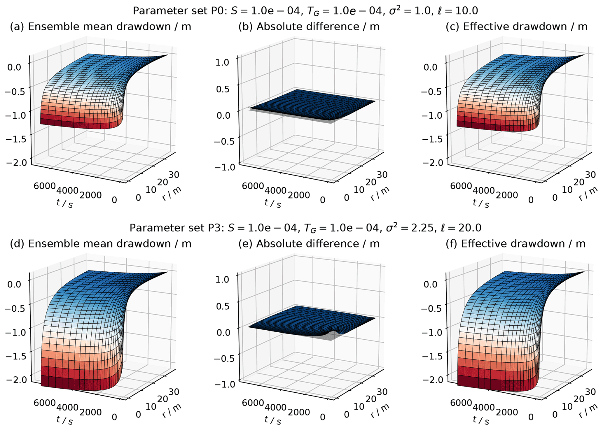
Figure 26Comparison the ensemble mean drawdown 〈h(r,t)〉 (a, d) with the effective head solution hCG(r,t) (c, f) for two parameter sets. The vanishing absolute difference between both (b, e) shows that they perfectly agree.
Figure 18 shows how to set up the UK estimator, including the drift function, and Fig. 19 shows the setup of the RK estimator. RK requires the preceding step of fitting the regression model for the trend of the Detrended kriging routine. The interpolation results are shown in Fig. 20, indicating that both methods provide equally good results.
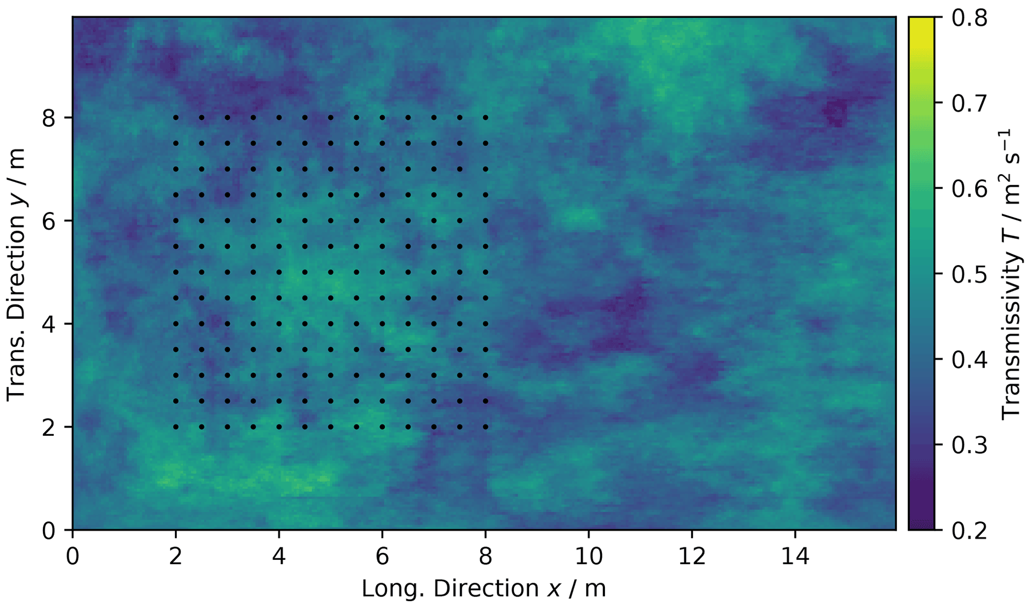
Figure 27Transmissivity of the Herten aquifer analogue and locations of virtual observations marked as black dots.
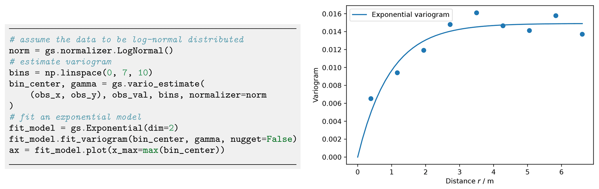
Figure 28Variogram estimation and resulting experimental (dots) and fitted variogram γ (line) of the Herten aquifer analogue.
Figure 21 shows the estimated mean trends for both UK and RK, revealing completely contrary results. The RK result indicates an increase in mean temperature with increasing latitude, which seems reasonable given a raising terrain elevation from the Baltic Sea in the north towards the Alps in the south. The estimated mean of UK shows the opposite with temperature decreasing with latitude. A potential explanation here is the general temperature increase towards the Equator. While the UK mean fits better with the cross-section at 10∘ longitude (Fig. 21), the RK mean fits the scatter diagram better, as expected.
4.2 Heterogeneous transport simulation: the impact of connectivity
The combination of ogs5py and GSTools makes it possible to quickly set up and run subsurface flow and transport simulations in a heterogeneous aquifer setting. The critical step is the generation of a spatially distributed hydraulic conductivity distribution, adapted to the numerical simulation grid. We further demonstrate GSTools' ability to generate different connectivity structures, and we discuss their impact on transport results.
The resources for this workflow are provided in Müller and Zech (2021a).
A flow and transport model is initialized through an instance of the OGS class from ogs5py, with simple mesh generation (Fig. 22) and specification of model parameters and boundary conditions.
Random fields are initialized through the SRF class (Fig. 23). By passing the subclass model.msh, mesh details are transferred for generating distributed values at particular mesh locations, even for unstructured grids.
The subroutine transform.zinnharvey allows for generating Gaussian structures where the mean values of the field are not connected but the low- or high-conductivity areas are connected, using the transformation by Zinn and Harvey (2003).
Note that the correlation lengths undergo rescaling (Gong et al., 2013).
The concept of connectivity follows the paper by Zinn and Harvey (2003), where connectedness refers to connected paths of extreme or special values in the conductivity field.

Figure 29One realization of the conditioned SRF (a) and absolute difference (b) between the “true” (Fig. 27) and conditioned transmissivity, showing increasing differences with distance from the conditioning area (rectangle).
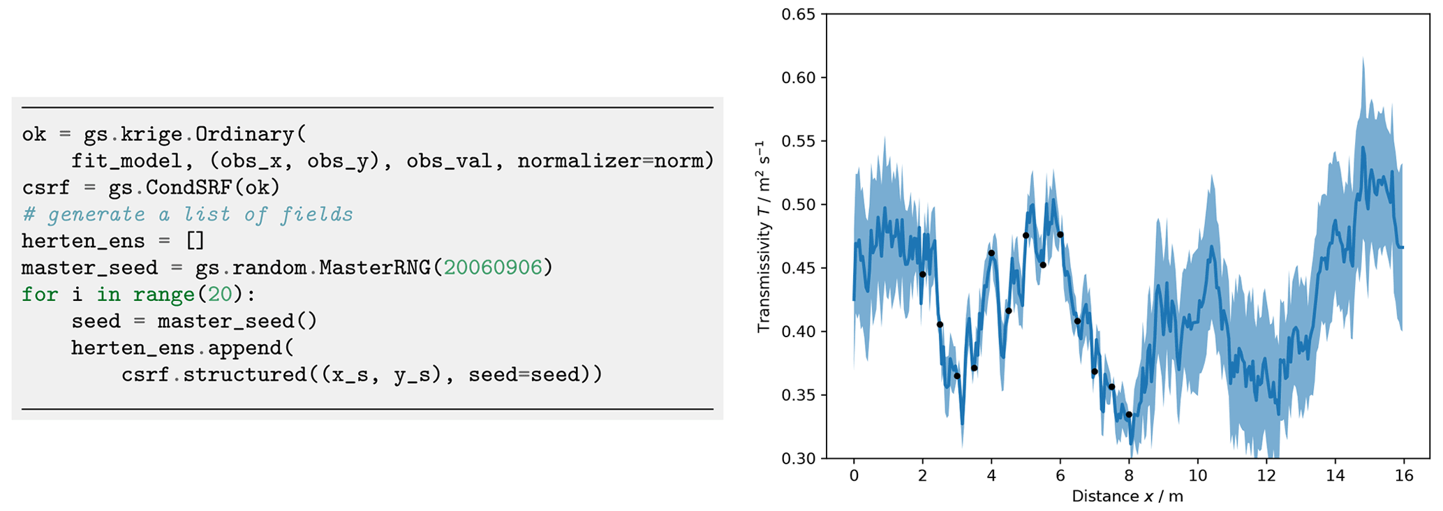
Figure 30Generation of an ensemble of 20 conditional realizations and transmissivity transects T(x) at y=4 m. The thick blue line is the true transmissivity (Fig. 27), and the shaded area shows the range of 1 standard deviation calculated from 20 realizations of conditioned fields. Black points indicate the observations.
Simulated tracer plumes in Fig. 24 show the particular effects of connectivity: the plume remains relatively compact for classical Gaussian fields, where mean values are connected. Transformed fields lead to more disrupted, dynamic plumes, which is mostly caused by trapping in areas of connected low conductivity and preferential flow in connected high-conductivity areas.
4.3 Characterizing mean drawdowns of a pumping test ensemble
Combining flow simulations in ogs5py with random fields of GSTools allows for performing Monte Carlo studies to identify ensemble mean behaviour.
Zech et al. (2016) made use of this workflow to prove the applicability of an effective drawdown solution for pumping tests in random conductivity. We present a short form of their workflow, which is accessible in Müller and Zech (2021b).
The flow model is initialized through the OGS class with model parameters and boundary conditions creating the convergent flow setting of a pumping test.
The mesh generation and time stepping can be specifically adapted to the non-uniform flow conditions. Ensembles of heterogeneous transmissivity fields are generated with the SRF class where reproducibility is controlled by the seed and where normal fields are converted in place with normalizer.LogNormal as shown in Fig. 25.
The implementation of the randomization method (Sect. 2.2.2) allows for the adaption of random fields to the non-uniform grid. The associated variance upscaling follows the coarse graining procedure for Gaussian variograms according to Eq. (20).
Calculated ensemble means can be compared to analytical solutions (Fig. 26), such as Theis' solution for homogeneous media or the effective drawdown solution by Zech et al. (2016), making use of their implementations in welltestpy and AnaFlow.
4.4 Geostatistical exercises with the Herten aquifer
We demonstrate how to estimate variograms and how to condition spatial random fields on observations using data from the Herten aquifer analogue (Bayer et al., 2011). The aquifer analogue was created from surveying multiple outcrop faces at a gravel pit, situated in the Rhine valley in southern Germany. The 2D information was interpolated to a 3D data set, including hydraulic, thermal and chemical information. The workflow files are provided in Schüler and Müller (2021).
We determine spatial correlations through variogram estimation using gstools.variogram.
First, we identify the full transmissivity structure. The aquifer analogue data are given in a facies structure with one hydraulic conductivity value K per facies. We calculate transmissivity by integrating the hydraulic conductivity over the vertical axis . The structured transmissivity is shown in Fig. 27, which we consider as true distribution for the following exercises.
We select 13×13 virtual observations on a rectangular grid (Fig. 27), covering a subarea of about 42 m2. These observations are used to determine the empirical variogram shown in Fig. 28. We fit an exponential covariance model to the data, which suits well with a coefficient of determination of R2=0.913.
We use the fitted exponential variogram model and ordinary kriging to create conditioned spatial random fields with CondSRF.
Figure 29 shows one realization and the absolute difference to the true transmissivity (Fig. 27). Differences grow with increasing distance from observations.
This trend can be even better seen in a transmissivity transect shown in Fig. 30. The standard deviation calculated from 20 realizations of conditioned SRFs shows that deviations from the reference field are significantly lower close to observation points.
The GSTools package provides a Python-based platform for geostatistical applications.
It is similar to software packages like gstat for R or stand-alone packages like TPROGS (Carle, 1999), GSLIB (Deutsch and Journel, 1997) and S-GeMS (Remy, 2005).
However, we believe that a comprehensive and ready-made geostatistical software package for Python has advantages, simply through the choice of the programming language, as it has a gentle learning curve, is often used as a glue language and is widely adopted by the scientific community.
Salient features of GSTools are its random field generation and its versatile covariance model.
It is furthermore integrated with other Python packages, like PyKrige (Murphy et al., 2021), ogs5py (Müller et al., 2020) or scikit-gstat (Mälicke, 2022), and provides interfaces to meshio (Schlömer et al., 2021) and PyVista (Sullivan and Kaszynski, 2019).
GeoStat Examples (https://github.com/GeoStat-Examples, last access: 31 March 2022) provides a number of applications, including the four presented workflows. They showcase the abilities of GSTools and can serve as a starting point for practitioners to develop their own solutions for the geostatistical problems they face.
As part of the GeoStat Framework, the code of GSTools is developed at https://github.com/GeoStat-Framework/GSTools and available via Zenodo at https://doi.org/10.5281/zenodo.5883346 (Müller and Schüler, 2021).
It is distributed under the GNU LGPL v3.0 licence.
The documentation, which includes a quick-start guide, some more in-depth tutorials and a complete overview over the API, can be accessed via https://gstools.readthedocs.io/ (last access: 31 March 2022).
The workflows can be found in separate repositories https://github.com/GeoStat-Examples/gstools-temperature-trend, (Müller, 2021), https://github.com/GeoStat-Examples/gstools-connectivity-and-transport, (Müller and Zech, 2021a), https://github.com/GeoStat-Examples/gstools-pumping-test-ensemble, (Müller and Zech, 2021b), https://github.com/GeoStat-Examples/gstools-herten-example, and (Schüler and Müller, 2021).
All data can be accessed by the given DOIs (https://doi.org/10.5281/zenodo.5159728, Müller, 2021, https://doi.org/10.5281/zenodo.5159578, Müller and Zech, 2021a, https://doi.org/10.5281/zenodo.4891875, Müller and Zech, 2021b, https://doi.org/10.5281/zenodo.5159658, Schüler and Müller, 2021) and the related repositories are hosted under https://github.com/GeoStat-Examples (last access: 31 March 2022).
SM and LS are the main authors of the GSTools package, with contributions by Falk Heße to an older version of the package.
SM, LS and AZ contributed to the implementation of the workflows.
AZ acted as supervisor for SM with respect to the scientific applications of GSTools (workflows).
The article was collectively written by SM, FH, AZ and LS with major contributions by SM.
The contact author has declared that neither they nor their co-authors have any competing interests.
Publisher’s note: Copernicus Publications remains neutral with regard to jurisdictional claims in published maps and institutional affiliations.
We would like to thank everyone who contributed to GSTools and all the people using it and asking questions about it. We want to especially thank Mirko Mälicke for the good cooperation to make SciKit-GStat and GSTools work together harmoniously and complement each other.
Sebastian Müller and Falk Heße were financially supported by the Deutsche Forschungsgemeinschaft via grant number HE-7028-1/2.
Sebastian Müller was also funded by the German Federal Environmental Foundation (grant no. 20016/432). This work was partially funded by the Center of Advanced Systems Understanding (CASUS), which is financed by Germany's Federal Ministry of Education and Research (BMBF) and by the Saxon Ministry for Science, Culture and Tourism (SMWK) with tax funds on the basis of the budget approved by the Saxon State Parliament.
The article processing charges for this open-access publication were covered by the Helmholtz Centre for Environmental Research – UFZ.
This paper was edited by Fabien Maussion and reviewed by two anonymous referees.
Abramowitz, M., and Stegun, I. A.: Handbook of mathematical functions, 10th edn., Dover Publications, New York, ISBN 978-0-486-61272-0, 1972. a
Attinger, S.: Generalized coarse graining procedures for flow in porous media, Computat. Geosci., 7, 253–273, https://doi.org/10.1023/B:COMG.0000005243.73381.e3, 2003. a
Banerjee, S., Carlin, B. P., and Gelfand, A. E.: Hierarchical Modeling and Analysis for Spatial Data, 2 edn., Chapman and Hall/CRC, Boca Raton, https://doi.org/10.1201/b17115, 2014. a
Bayer, P., Huggenberger, P., Renard, P., and Comunian, A.: Three-dimensional high resolution fluvio-glacial aquifer analog: Part 1: Field study, J. Hydrol., 405, 1–9, https://doi.org/10.1016/j.jhydrol.2011.03.038, 2011. a
Beg, M., Taka, J., Kluyver, T., Konovalov, A., Ragan-Kelley, M., Thiéry, N. M., and Fangohr, H.: Using Jupyter for Reproducible Scientific Workflows, in: Computing in Science Engineering, Computing in Science Engineering, 23, 36–46, https://doi.org/10.1109/MCSE.2021.3052101, 2021. a
Behnel, S., Bradshaw, R., Citro, C., Dalcin, L., Seljebotn, D. S., and Smith, K.: Cython: The Best of Both Worlds, in: Computing in Science Engineering, Computing in Science Engineering, 13, 31–39, https://doi.org/10.1109/MCSE.2010.118, 2011. a
Bellin, A. and Rubin, Y.: HYDRO_GEN: A spatially distributed random field generator for correlated properties, Stoch. Hydrol. Hydraul., 10, 253–278, https://doi.org/10.1007/BF01581869, 1996. a
Box, G. E. P. and Cox, D. R.: An Analysis of Transformations, J. Roy. Stat. Soc. B, 26, 211–243, https://doi.org/10.1111/j.2517-6161.1964.tb00553.x, 1964. a, b
Brouste, A., Istas, J., and Lambert-Lacroix, S.: On Fractional Gaussian Random Fields Simulations, J. Stat. Softw., 23, 1–23, https://doi.org/10.18637/jss.v023.i01, 2008. a
Carle, S. F.: T-PROGS: Transition probability geostatistical software, version 2.1, Tech. Rep., University of California, Davis, http://gmsdocs.aquaveo.com/t-progs.pdf (last access: 31 March 2022), 1999. a
Cecinati, F., Wani, O., and Rico-Ramirez, M. A.: Comparing Approaches to Deal With Non-Gaussianity of Rainfall Data in Kriging-Based Radar-Gauge Rainfall Merging, Water Resour. Res., 53, 8999–9018, https://doi.org/10.1002/2016WR020330, 2017. a, b
Chilès, J.-P. and Delfiner, P.: Geostatistics: Modeling Spatial Uncertainty, second edn., Wiley Series in Probability and Statistics, edited by: Balding, D. J., Cressie, N. A. C., Fitzmaurice, G. M., Goldstein, H., Johnstone, I. M., Molenberghs, G., Scott, D. W., Smith, A. F. M., Tsay, R. S., and Weisberg, S., John Wiley & Sons, https://doi.org/10.1002/9781118136188, 2012. a, b
Cirpka, O. A. and Valocchi, A. J.: Debates – Stochastic subsurface hydrology from theory to practice: Does stochastic subsurface hydrology help solving practical problems of contaminant hydrogeology?, Water Resour. Res., 52, 9218–9227, https://doi.org/10.1002/2016WR019087, 2016. a
conda-forge community: The conda-forge Project: Community-based Software Distribution Built on the conda Package Format and Ecosystem, Zenodo [software], https://doi.org/10.5281/zenodo.4774217, 2015. a
Cressie, N. and Wikle, C. K.: Statistics for spatio-temporal data, Wiley Series in Probability and Statistics, 1st edn., John Wiley & Sons, Hoboken, New Jersey, ISBN 978-0-471-69274-4, 2011. a
Dagan, G.: Flow and Transport in Porous Formations, 1st edn., Springer, Berlin, Heidelberg, https://doi.org/10.1007/978-3-642-75015-1, 1989. a
Deutsch, C. V. and Journel, A. G.: GSLIB: Geostatistical software library and user's guide, Applied geostatistics series, 2. edn., Oxford University Press, ISBN 9780195100150, 1997. a, b
Di Federico, V. and Neuman, S. P.: Scaling of random fields by means of truncated power variograms and associated spectra, Water Resour. Res., 33, 1075–1085, https://doi.org/10.1029/97WR00299, 1997. a, b, c
Diggle, P. and Ribeiro, P. J.: Model-based Geostatistics, Springer Series in Statistics, 1st edn., Springer-Verlag, New York, https://doi.org/10.1007/978-0-387-48536-2, 2007. a
Eliason, S. R.: Maximum likelihood estimation: Logic and practice, Sage Publications, 1st edn., Thousand Oaks, CA, US, ISBN 9781506315904, 1993. a
Emery, X.: Testing the correctness of the sequential algorithm for simulating Gaussian random fields, Stoch. Env. Res. Risk A., 18, 401–413, https://doi.org/10.1007/s00477-004-0211-7, 2004. a
Fiori, A., Cvetkovic, V., Dagan, G., Attinger, S., Bellin, A., Dietrich, P., Zech, A., and Teutsch, G.: Debates – Stochastic subsurface hydrology from theory to practice: The relevance of stochastic subsurface hydrology to practical problems of contaminant transport and remediation. What is characterization and stochastic theory good for?, Water Resour. Res., 52, 9228–9234, https://doi.org/10.1002/2015WR017525, 2016. a
Foreman-Mackey, D., Hogg, D. W., Lang, D., and Goodman, J.: emcee: The MCMC Hammer, Publ. Astron. Soc. Pac., 125, 306–312, https://doi.org/10.1086/670067, 2013. a
Goldstein, H.: Classical mechanics, 2nd edn., Addison-Wesley, ISBN 9780201029185, 1980. a
Gong, R., Haslauer, C. P., Chen, Y., and Luo, J.: Analytical relationship between Gaussian and transformed-Gaussian spatially distributed fields, Water Resour. Res., 49, 1735–1740, https://doi.org/10.1002/wrcr.20143, 2013. a
Goovaerts, P.: Geostatistics in soil science: state-of-the-art and perspectives, Geoderma, 89, 1–45, https://doi.org/10.1016/S0016-7061(98)00078-0, 1999. a
Gutzmann, B., Motl, A., Lassahn, D., Kamenshchikov, I., Bachmann, M., and Schrammel, M.: earthobservations/wetterdienst: v0.18.0, Zenodo [software], https://doi.org/10.5281/zenodo.4737739, 2021. a
Harris, C. R., Millman, K. J., van der Walt, S. J., Gommers, R., Virtanen, P., Cournapeau, D., Wieser, E., Taylor, J., Berg, S., Smith, N. J., Kern, R., Picus, M., Hoyer, S., van Kerkwijk, M. H., Brett, M., Haldane, A., Fernández del Río, J., Wiebe, M., Peterson, P., Gérard-Marchant, P., Sheppard, K., Reddy, T., Weckesser, W., Abbasi, H., Gohlke, C., and Oliphant, T. E.: Array programming with NumPy, Nature, 585, 357–362, https://doi.org/10.1038/s41586-020-2649-2, 2020. a
Heße, F., Prykhodko, V., Schlüter, S., and Attinger, S.: Generating random fields with a truncated power-law variogram: A comparison of several numerical methods, Environ. Modell. Softw., 55, 32–48, https://doi.org/10.1016/j.envsoft.2014.01.013, 2014. a, b, c
Hohn, M.: Geostatistics and Petroleum Geology, Computer Methods in the Geosciences, 2 edn., Springer Netherlands, https://doi.org/10.1007/978-94-011-4425-4, 1999. a
John, J. A. and Draper, N. R.: An Alternative Family of Transformations, J. Roy. Stat. Soc. C-App., 29, 190–197, https://doi.org/10.2307/2986305, 1980. a
Kitanidis, P.: Introduction to Geostatistics: Applications in Hydrogeology, 1st edn., Cambridge University Press, Cambridge, New York, ISBN 9780521587471, 2008. a, b
Kolditz, O., Bauer, S., Bilke, L., Böttcher, N., Delfs, J.-O., Fischer, T., Görke, U. J., Kalbacher, T., Kosakowski, G., McDermott, C. I., Park, C. H., Radu, F., Rink, K., Shao, H., Shao, H. B., Sun, F., Sun, Y. Y., Singh, A. K., Taron, J., Walther, M., Wang, W., Watanabe, N., Wu, Y., Xie, M., Xu, W., and Zehner, B.: OpenGeoSys: An open-source initiative for numerical simulation of thermo-hydro-mechanical/chemical (THM/C) processes in porous media, Environ. Earth Sci., 67, 589–599, https://doi.org/10.1007/s12665-012-1546-x, 2012. a
Kraichnan, R.: Diffusion by a Random Velocity Field, Phys. Fluids, 13, 22–31, https://doi.org/10.1063/1.1692799, 1970. a, b, c
Krige, D. G.: A statistical approach to some basic mine valuation problems on the Witwatersrand, J. S. Afr. I. Min. Metall., 52, 119–139, 1951. a
Lantuéjoul, C., Freulon, X., and Renard, D.: Spectral Simulation of Isotropic Gaussian Random Fields on a Sphere, Math. Geosci., 51, 999–1020, https://doi.org/10.1007/s11004-019-09799-4, 2019. a
Mälicke, M.: SciKit-GStat 1.0: a SciPy-flavored geostatistical variogram estimation toolbox written in Python, Geosci. Model Dev., 15, 2505–2532, https://doi.org/10.5194/gmd-15-2505-2022, 2022. a, b
Manly, B. F. J.: Exponential Data Transformations, J. Roy. Stat. Soc. D-Sta., 25, 37–42, https://doi.org/10.2307/2988129, 1976. a
Matheron, G.: Traité de géostatistique appliquée, no. 14 in Mémoires du BRGM, Editions Technip, Tome II: le krigeage, no 24, Editions BRGM, Paris, 1962. a
Matern, B.: Spatial variation – stochastic models and their applications to some problems in forest survey sampling investigations, Report of the Forest Research Institute of Sweden 49, 1–144, 1960 (in English, Swedish summary). a, b
Mohammadi, H., Riche, R. L., Durrande, N., Touboul, E., and Bay, X.: An analytic comparison of regularization methods for Gaussian Processes, arXiv [preprint], arXiv:1602.00853, 5 May 2017. a
Monestiez, P., Petrenko, A., Leredde, Y., and Ongari, B.: Geostatistical analysis of three dimensional current patterns in coastal oceanography: Application to the gulf of lions (NW mediterranean sea), in: geoENV IV – Geostatistics for environmental applications, edited by: Sanchez-Vila, X., Carrera, J., and Gómez-Hernández, J. J., pp. 367–378, Springer Netherlands, Dordrecht, https://doi.org/10.1007/1-4020-2115-1_31, 2004. a
Müller, S.: GeoStat – Examples/gstools-temperature-trend: v1.0, Zenodo [data set], https://doi.org/10.5281/zenodo.5159728, 2021. a, b, c
Müller, S. and Schüler, L.: GeoStat – Framework/GSTools: v1.3.5 “Pure Pink”, Zenodo [code], https://doi.org/10.5281/zenodo.5883346, 2021. a, b
Müller, S. and Zech, A.: GeoStat – Examples/gstools-connectivity-and-transport: v1.0, Zenodo [data set], https://doi.org/10.5281/zenodo.5159578, 2021a. a, b, c
Müller, S. and Zech, A.: GeoStat – Examples/gstools-pumping-test-ensemble: v1.0, Zenodo [data set], https://doi.org/10.5281/zenodo.4891875, 2021b. a, b, c
Müller, S., Zech, A., and Heße, F.: ogs5py: A Python – API for the OpenGeoSys 5 Scientific Modeling Package, Groundwater, 59, 117–122, https://doi.org/10.1111/gwat.13017, 2020. a, b, c
Müller, S., Heße, F., Attinger, S., and Zech, A.: The extended generalized radial flow model and effective conductivity for truncated power law variograms, Adv. Water Resour., 156, 104027, https://doi.org/10.1016/j.advwatres.2021.104027, 2021a. a, b
Müller, S., Leven, C., Dietrich, P., Attinger, S., and Zech, A.: How to Find Aquifer Statistics Utilizing Pumping Tests? Two Field Studies Using welltestpy, Groundwater, 60, 137–144, https://doi.org/10.1111/gwat.13121, 2021b. a
Murphy, B., Müller, S., and Yurchak, R.: GeoStat-Framework/PyKrige: v1.6.0, Zenodo [code], https://doi.org/10.5281/zenodo.4661732, 2021. a, b
Murray, S. G. and Poulin, F. J.: hankel: A Python library for performing simple and accurate Hankel transformations, The Journal of Open Source Software, 4, 1397, https://doi.org/10.21105/joss.01397, 2019. a
Neuman, S. P.: Stochastic groundwater models in practice, Stoch. Env. Res. Risk A., 18, 268–270, https://doi.org/10.1007/s00477-004-0192-6, 2004. a
Ogata, H.: A Numerical Integration Formula Based on the Bessel Functions, Publ. Res. I. Math. Sci., 41, 949–970, https://doi.org/10.2977/prims/1145474602, 2005. a
Pebesma, E. J.: Multivariable geostatistics in S: the gstat package, Comput. Geosci., 30, 683–691, https://doi.org/10.1016/j.cageo.2004.03.012, 2004. a
Perkel, J. M.: Why Jupyter is data scientists’ computational notebook of choice, Nature, 563, 145–146, https://doi.org/10.1038/d41586-018-07196-1, 2018. a
Pyrcz, M. J. and Deutsch, C. V.: Geostatistical Reservoir Modeling, 2 edn., Oxford University Press, Oxford, ISBN 978-0199731442, 2014. a
Queiroz, F., Silva, R., Miller, J., Brockhauser, S., and Fangohr, H.: Track 1 Paper: Good Usability Practices in Scientific Software Development, Figshare, https://doi.org/10.6084/m9.figshare.5331814.v3, 2017. a
Rajaram, H.: Debates – Stochastic subsurface hydrology from theory to practice: Introduction, Water Resour. Res., 52, 9215–9217, https://doi.org/10.1002/2016WR020066, 2016. a, b
Rasmussen, C. E. and Williams, C. K. I.: Gaussian Processes for Machine Learning, 1st edn., The MIT Press, ISBN 9780262256834, https://doi.org/10.7551/mitpress/3206.001.0001, 2005. a, b
Remy, N.: S-GeMS: The Stanford Geostatistical Modeling Software: A Tool for New Algorithms Development, in: Quantitative Geology and Geostatistics, Geostatistics Banff 2004, 14, 865–871, https://doi.org/10.1007/978-1-4020-3610-1_89, 2005. a, b
Rossi, R. E., Mulla, D. J., Journel, A. G., and Franz, E. H.: Geostatistical tools for modeling and interpreting ecological spatial dependence, Ecol. Monogr., 62, 277–314, https://doi.org/10.2307/2937096, 1992. a
Rubin, Y.: Applied Stochastic Hydrogeology, 1st edn., Oxford University Press, New York, ISBN 9780195138047, https://doi.org/10.1093/oso/9780195138047.001.0001, 2003. a, b, c, d
Rubin, Y., Chen, X., Murakami, H., and Hahn, M.: A Bayesian approach for inverse modeling, data assimilation, and conditional simulation of spatial random fields, Water Resour. Res., 46, W10523, https://doi.org/10.1029/2009WR008799, 2010. a
Rubin, Y., Chang, C.-F., Chen, J., Cucchi, K., Harken, B., Heße, F., and Savoy, H.: Stochastic hydrogeology's biggest hurdles analyzed and its big blind spot, Hydrol. Earth Syst. Sci., 22, 5675–5695, https://doi.org/10.5194/hess-22-5675-2018, 2018. a, b
Rudin, W.: Fourier Analysis on Groups, 1st edn., Wiley‐Interscience, John Wiley & Sons, ISBN 9780470744819, https://doi.org/10.1002/9781118165621, 1990. a
Sales, M. H., Souza, C. M., Kyriakidis, P. C., Roberts, D. A., and Vidal, E.: Improving spatial distribution estimation of forest biomass with geostatistics: A case study for Rondônia, Brazil, Ecol. Model., 205, 221–230, https://doi.org/10.1016/j.ecolmodel.2007.02.033, 2007. a
Savoy, H., Heße, F., and Rubin, Y.: anchoredDistr: a Package for the Bayesian Inversion of Geostatistical Parameters with Multi-type and Multi-scale Data, R Journal, 9, 6–17, https://doi.org/10.32614/RJ-2017-034, 2017. a
Schlömer, N., McBain, G. D., Luu, K., christos, Li, T., Hochsteger, M., Keilegavlen, E., Ferrándiz, V. M., Barnes, C., Lukeš, V., Dalcin, L., Jansen, M., Wagner, N., Gupta, A., Müller, S., Woodsend, B., Andersen, K., Schwarz, L., Blechta, J., Christovasilis, I. P., Coutinho, C., Beurle, D., ffilotto, Dokken, J. S., blacheref, so1291, Cervone, A., Shrimali, B., Bill, and Jones, D.: nschloe/meshio: None, Zenodo [code], https://doi.org/10.5281/zenodo.4900671, 2021. a, b
Schüler, L. and Müller, S.: GeoStat – Examples/gstools-herten-example: v1.0, Zenodo [data set], https://doi.org/10.5281/zenodo.5159658, 2021. a, b, c
Schüler, L., Suciu, N., Knabner, P., and Attinger, S.: A time dependent mixing model to close PDF equations for transport in heterogeneous aquifers, Adv. Water Resour., 96, 55–67, https://doi.org/10.1016/j.advwatres.2016.06.012, 2016. a
Schüler, L., Calabrese, J. M., and Attinger, S.: Data driven high resolution modeling and spatial analyses of the COVID-19 pandemic in Germany, PLOS ONE, 16, 1–14, https://doi.org/10.1371/journal.pone.0254660, 2021. a
Sturges, H. A.: The Choice of a Class Interval, J. Am. Stat. Assoc., 21, 65–66, https://doi.org/10.1080/01621459.1926.10502161, 1926. a
Sullivan, C. B. and Kaszynski, A. A.: PyVista: 3D plotting and mesh analysis through a streamlined interface for the Visualization Toolkit (VTK), Journal of Open Source Software, 4, 1450, https://doi.org/10.21105/joss.01450, 2019. a, b
Uieda, L.: Verde: Processing and gridding spatial data using Green’s functions, Journal of Open Source Software, 3, 957, https://doi.org/10.21105/joss.00957, 2018. a
Virtanen, P., Gommers, R., Oliphant, T. E., Haberland, M., Reddy, T., Cournapeau, D., Burovski, E., Peterson, P., Weckesser, W., Bright, J., van der Walt, S. J., Brett, M., Wilson, J., Millman, K. J., Mayorov, N., Nelson, A. R. J., Jones, E., Kern, R., Larson, E., Carey, C. J., Polat, i., Feng, Y., Moore, E. W., VanderPlas, J., Laxalde, D., Perktold, J., Cimrman, R., Henriksen, I., Quintero, E. A., Harris, C. R., Archibald, A. M., Ribeiro, A. H., Pedregosa, F., van Mulbregt, P., and SciPy 1.0 Contributors: SciPy 1.0: Fundamental algorithms for scientific computing in python, Nat. Methods, 17, 261–272, https://doi.org/10.1038/s41592-019-0686-2, 2020. a
Vrugt, J. A.: Markov chain Monte Carlo simulation using the DREAM software package: Theory, concepts, and MATLAB implementation, Environ. Modell. Softw., 75, 273–316, https://doi.org/10.1016/j.envsoft.2015.08.013, 2016. a
Wackernagel, H.: Multivariate Geostatistics: An Introduction with Applications, 3 edn., Springer-Verlag, Berlin Heidelberg, ISBN 978-3-540-44142-7, https://doi.org/10.1007/978-3-662-05294-5, 2003. a, b, c, d
Webster, R. and Oliver, M. A.: Geostatistics for Environmental Scientists, 2 edn., John Wiley & Sons, ISBN 978-0-470-02858-2, 2007. a, b, c, d, e, f, g, h
Wendland, H.: Piecewise polynomial, positive definite and compactly supported radial functions of minimal degree, Adv. Comput. Math., 4, 389–396, https://doi.org/10.1007/BF02123482, 1995. a
Winter, C. L.: Stochastic hydrology: practical alternatives exist, Stoch. Env. Res. Risk A., 18, 271–273, https://doi.org/10.1007/s00477-004-0198-0, 2004. a
Yeo, I. and Johnson, R. A.: A new family of power transformations to improve normality or symmetry, Biometrika, 87, 954–959, https://doi.org/10.1093/biomet/87.4.954, 2000. a
Zech, A., Schneider, C. L., and Attinger, S.: The extended Thiem's solution – Including the impact of heterogeneity, Water Resour. Res., 48, W10535, https://doi.org/10.1029/2012WR011852, 2012. a
Zech, A., Müller, S., Mai, J., Heße, F., and Attinger, S.: Extending Theis' solution: Using transient pumping tests to estimate parameters of aquifer heterogeneity, Water Resour. Res., 52, 6156–6170, https://doi.org/10.1002/2015WR018509, 2016. a, b, c
Zhang, Y.-K. and Zhang, D.: Forum: The state of stochastic hydrology, Stoch. Env. Res. Risk A., 18, 265, https://doi.org/10.1007/s00477-004-0190-8, 2004. a, b
Zinn, B. and Harvey, C. F.: When good statistical models of aquifer heterogeneity go bad: A comparison of flow, dispersion, and mass transfer in connected and multivariate Gaussian hydraulic conductivity fields, Water Resour. Res., 39, 1051, https://doi.org/10.1029/2001WR001146, 2003. a, b, c, d