the Creative Commons Attribution 4.0 License.
the Creative Commons Attribution 4.0 License.
 | 23 Mar 2022
Analysing the PMIP4-CMIP6 collection: a workflow and tool (pmip_p2fvar_analyzer v1)
Chris M. Brierley
Zhiyi Jiang
Rachel Eyles
Damián Oyarzún
Jose Gomez-Dans
Experiment outputs are now available from the Coupled Model Intercomparison Project's sixth phase (CMIP6) and the past climate experiments defined in the Palaeoclimate Modelling Intercomparison Project's fourth phase (PMIP4). All of this output is freely available from the Earth System Grid Federation (ESGF). Yet there is overhead in analysing this resource that may prove complicated or prohibitive. Here we document the steps taken by ourselves to produce ensemble analyses covering past and future simulations. We outline the strategy used to curate, adjust the monthly calendar aggregation and process the information downloaded from the ESGF. The results of these steps were used to perform analysis for several of the initial publications arising from PMIP4. We provide post-processed fields for each simulation, such as climatologies and common measures of variability. Example scripts used to visualise and analyse these fields are provided for several important case studies.
- Article
(6696 KB) - Full-text XML
- BibTeX
- EndNote


Palaeoclimate modelling has long been used to understand the mechanisms of past climate changes and has also served as a tool to test the response of climate models to the out-of-sample boundary conditions and forcings like high atmospheric CO2 concentration that are used in future climate change projections (e.g. Harrison et al., 2014, 2015; Schmidt et al., 2014). Model intercomparison projects have become important in climate research and run multiple models under the same identical experimental design that helps to synthesise simulated climate change across models. The Palaeoclimate Modelling Intercomparison Project, now in its fourth phase (PMIP4; Kageyama et al., 2018), is a project endorsed by the Coupled Model Intercomparison Project phase 6 (CMIP6; Eyring et al., 2016), which aims to analyse and understand the differences between model simulations of past climates. PMIP4 has been updated from its earlier phase PMIP3 (Braconnot et al., 2012) by including additional past warm periods (Fig. 1), updated experimental designs and involvement of the new generation of climate models (Kageyama et al., 2018; Eyring et al., 2016).
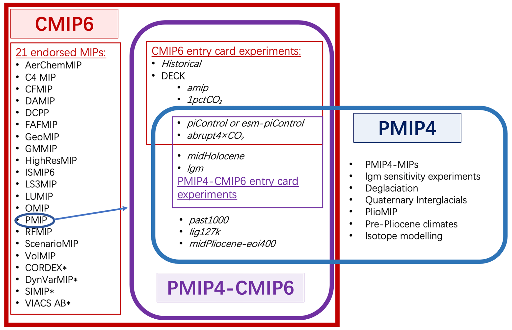
Figure 1Schematic diagram illustrating the CMIP6 and PMIP4 experiments after Eyring et al. (2016) and Kageyama et al. (2018). “CMIP6” refers to the phase of the Coupled Model Intercomparison Project devised to support the IPCC's Sixth Assessment Report. “PMIP4” is the fourth phase of the Palaeoclimate Modelling Intercomparison Project. We refer to the subset of models and experiments in PMIP4 that are also part of CMIP6 (purple) as “PMIP4-CMIP6”.
The Mid-Holocene (6000 years ago) and the Last Interglacial (127 000 years ago) are characterised by altered seasonal and latitudinal distribution of incoming solar radiation when the Earth's orbits were different from modern ones. The midHolocene and lig127k experiments are Tier 1 PMIP4-CMIP6 simulations (Fig. 1) designed to examine the model response to changes in the Earth's orbit in periods when the atmospheric greenhouse gas concentrations were similar to the preindustrial level and the topographies and ice sheet size were also similar to in modern times. Otto-Bliesner et al. (2017) described the protocols and specific information for the two experiments in detail. Brierley et al. (2020) summarised the large-scale features in the PMIP4-CMIP6 midHolocene simulations and the changes since the previous generation (PMIP3-CMIP5). Features in the PMIP4-CMIP6 lig127k ensemble have been analysed by Otto-Bliesner et al. (2021). These two ensembles within PMIP4 have contributed to the text in several chapters (Gulev et al., 2021; Eyring et al., 2021; Douville et al., 2022; Fox-Kemper et al., 2021) in the latest Sixth Assessment Report (AR6) of the Intergovernmental Panel on Climate Change (IPCC), as well as to figures in that report (Eyring et al., 2021).
PMIP4-CMIP6 model outputs have been standardised and uploaded on the Earth System Grid Federation (ESGF), servicing the diverse needs of various scientific communities (see Sect. 2 for more details). However, downloading these standardised files can be time-consuming due to abundant variables, their available various temporal resolutions, etc. Processing the files to conduct ensemble analysis can also be complicated because the simulations have differing time lengths and they use different spatial resolutions specific to the model configuration. Some methodological decisions are required through analysis. Therefore, a clear workflow and its saved outputs are useful for reducing the effort to download and process the PMIP4-CMIP6 outputs.
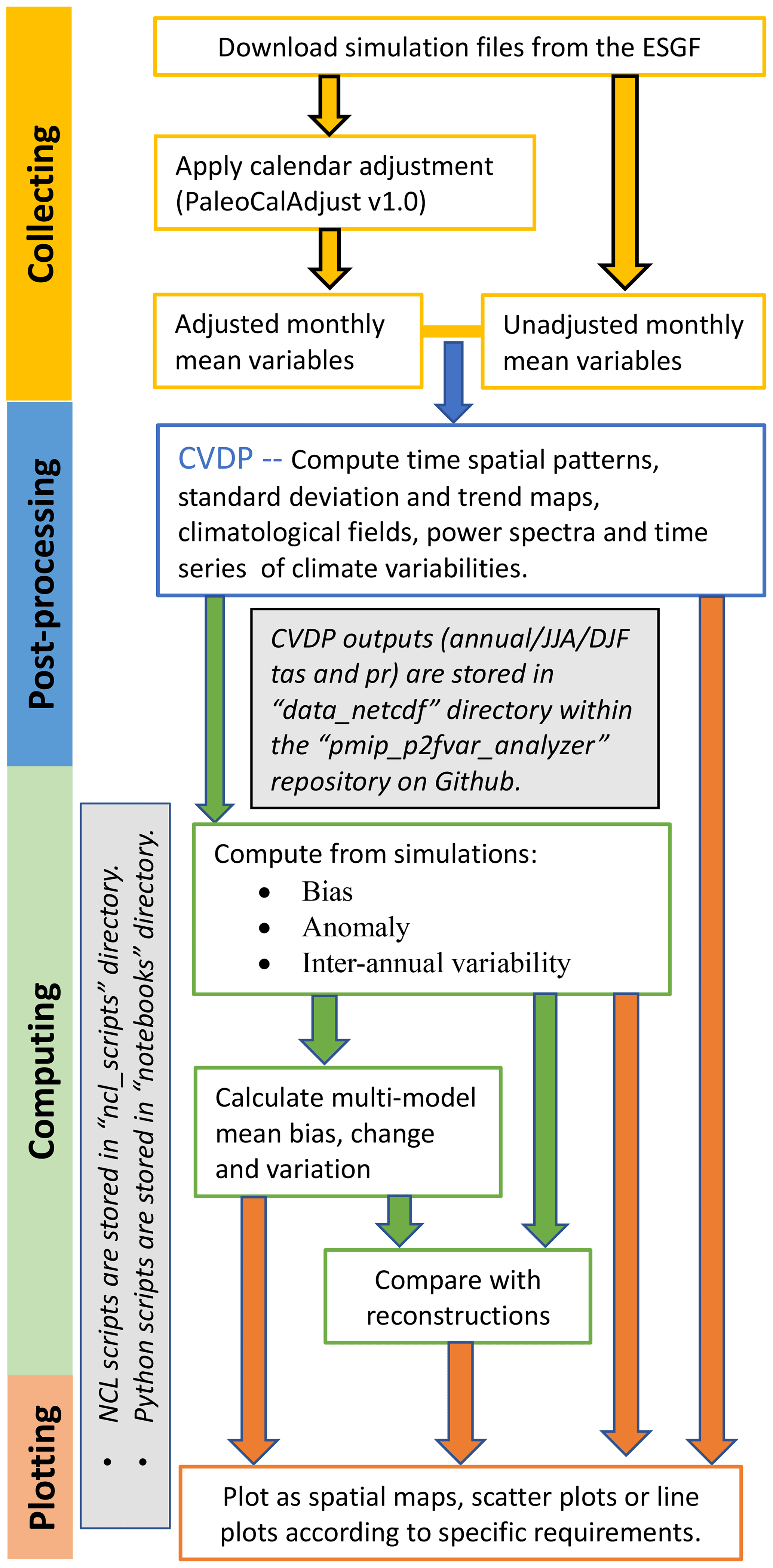
Here we provide a detailed description of the workflow (Fig. 2) and scripts that have been used to create figures in the primary description papers of the latest PMIP4-CMIP6 midHolocene (Brierley et al., 2020) and lig127k (Otto-Bliesner et al., 2021) experiments. The scripts have also been used for figures in multi-experiment papers coordinated by the Past2Future working group of PMIP on the PMIP3-CMIP5 tropical Atlantic interannual variability (Brierley and Wainer, 2018), PMIP3-CMIP5/6 climate variability (Rehfeld et al., 2020), and PMIP3-CMIP5 and PMIP4-CMIP6 El Niño–Southern Oscillation (ENSO) (Brown et al., 2020) and contributed to Figs. 3.2b and 3.11 in IPCC AR6 Working Group 1 (WG1), chap. 3 (Eyring et al., 2021). In Sect. 2, we give a description of the PMIP4 output availability and a discussion of how to access data, along with an evaluation of how and when to apply the PaleoCalAdjust software. The following section (Sect. 3) describes the Climate Variability Diagnostics Package (CVDP) and how it has been modified for PMIP4 purposes. The general NCL and Python routines (as pmip_p2fvar_analyzer v1.0) used in the above papers are described in detail in Sect. 4. Some case studies of possible analyses using the described workflow are given in Sect. 5, followed by a short summary in Sect. 6.
Each model participating in CMIP6 has uploaded (or is going to upload) their DECK and historical simulations (and endorsed MIP simulations if available) onto the Earth System Grid Federation (ESGF; Balaji et al., 2018, available at https://esgf-node.llnl.gov/search/cmip6/, last access: 17 December 2021) in the standard format as required by the CMIP6 Data Request (Juckes et al., 2020). All CMIP6 outputs have been written to netCDF files with one variable stored per file The number of variables and simulations contributed by each model is available at the ESGF CMIP6 PMIP Data Holdings web page (https://pcmdi.llnl.gov/CMIP6/ArchiveStatistics/esgf_data_holdings/PMIP/index.html, last access: 20 June 2021). Full lists of variables in the ESGF-controlled vocabulary are available at http://proj.badc.rl.ac.uk/svn/exarch/CMIP6dreq/tags/latest/dreqPy/docs/CMIP6_MIP_tables.xlsx (last access: 20 June 2021). Users can restrict searching results by selecting appropriate search constraints (e.g. Variable, Experiment ID and Frequency).
Table 1List of variables in the piControl, midHolocene and lig127k simulations that were downloaded from the ESGF.
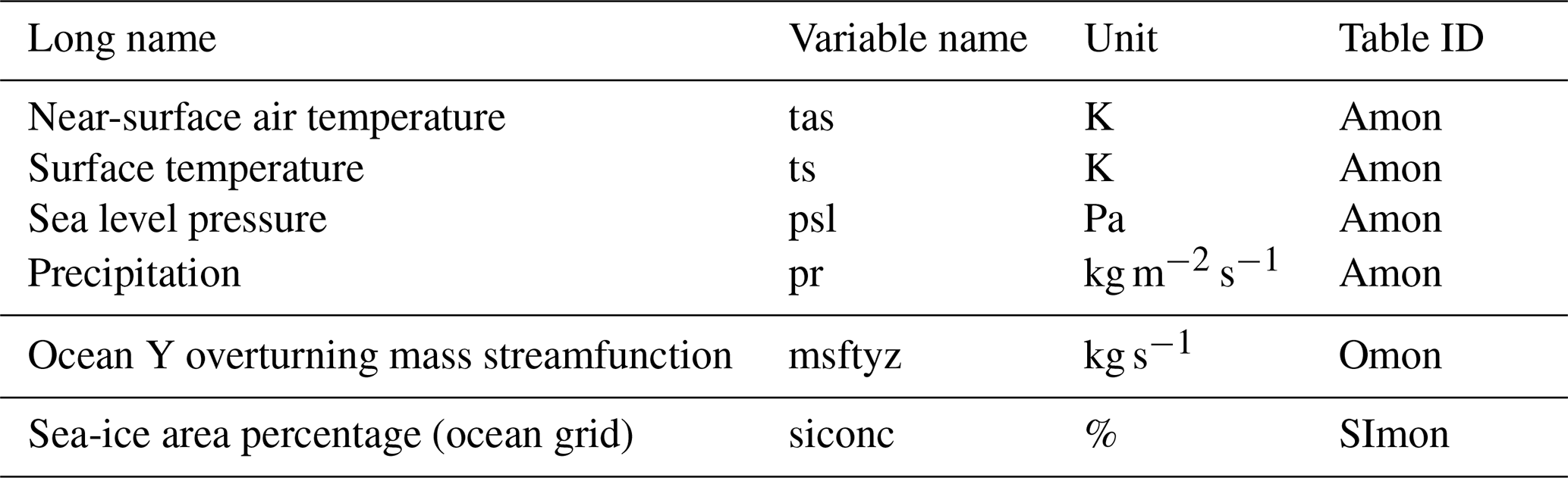
Information follows http://proj.badc.rl.ac.uk/svn/exarch/CMIP6dreq/tags/latest/dreqPy/docs/CMIP6_MIP_tables.xlsx (last access: 17 March 2022).
Table 1 lists the variables and their relevant information that we downloaded from the ESGF and used for analysis. For each PMIP model on the ESGF, data were acquired for every single experiment in the DECK and PMIP4 (see Fig. 1). Only a single variant was selected for each experiment. The variant ID of CMIP metadata is defined in a format of “r1i1p1f1”, where “r” is realisation, “i” is initialisation, “p” is physics, “f” is forcing and each number is the index for the corresponding configuration. Only FGOALS-g3 midHolocene has multiple runs, and r1i1p1f1 has been selected. There are four different forcings available for IPSL-CM6A-LR (Braconnot et al., 2019): only the r1i1p1f1 variant has been selected as that relates to the Tier 1 midHolocene protocol.
A local replica of the PMIP data stored on the ESGF was created to facilitate the deployment of the tools described later. The curation approach was chosen that permitted the inclusion of simulations prior to their publication on the ESGF and allowed for a coherent treatment calendar-adjusted files. Since each experiment contained a single ensemble member, a revised database structure was adopted to harmonise both CMIP6 and CMIP5 collection conventions. The resulting database has only two directory levels: the top level is taken as the model, with a sub-directory for each experiment that contains all the outputs listed in Table 1. Additionally an “areacello” (i.e. grid-cell area for ocean variables) fixed variable is stored in each sub-directory for the computation of sea ice area on rotated grids. This was not always deposited on the ESGF for an experiment and needed to be sourced from elsewhere. This curation approach has the added advantage of permitting manual treatment of individual issues. Symbolic links were used to populate this curated ESGF replica where possible (to avoid the duplication of data files). When many little files were stored on the ESGF, these were concatenated into a single larger file using the netCDF Operators (Zender, 2008) to avoid I/O bottlenecks. Only years for which all output variables are available were used. This curation approach had the additional advantage of permitting the inclusion of simulations prior to publication on the ESGF and allowed for a coherent treatment of calendar-adjusted files. The filenames of the resulting curated directory can be seen at https://github.com/pmip4/UCL_curated_ESGF_replica (last access: 17 March 2022).
The eccentricity, obliquity and precession in the Mid-Holocene and the Last Interglacial were different from those at 1850 CE. Therefore aggregating daily output to monthly averages using a “fixed-length” calendar to define the number of days in each month is not appropriate across all the experiments: a “fixed-angular” calendar should be used instead. Bartlein and Shafer (2019) provide software, PaleoCalAdjust, to convert between the two calendars for simulation output that is produced and stored in the general CMIP format. The approach taken by the PaleoCalAdjust software is to interpolate from non-adjusted monthly averages down to pseudo-daily values and then to aggregate those values back up to a “monthly” resolution for each 30∘ segment of Earth's orbit (see adjusted_month_lengths.xlsx on GitHub for adjusted month lengths). Bartlein and Shafer (2019) evaluated the software's performance for monthly temperature and precipitation variations and showed that in some situations the aliases due to the calendar definition can be larger than the climate change signal. Therefore, Brierley et al. (2020) and Otto-Bliesner et al. (2021) decided to apply the calendar adjustment when analysing seasonal temperature and precipitation. Calculation of regional mean temperature of the warmest month (MTWA) and of the coldest month (MTCO) for the Mid-Holocene in Fig. 3.44 in IPCC AR6 WG1 (Eyring et al., 2021) used adjusted monthly temperatures.
Brierley et al. (2020) explored the potential interpolation errors from PaleoCalAdjust for precipitation in monsoon regions (Pollard and Reusch, 2002) by analysing the averaged rain rate during the monsoon season over the South American monsoon domain in the IPSL-CM6A-LR midHolocene experiment. As a result, Brierley et al. (2020) decided to not apply the calendar adjustment when analysing monsoon variables while presenting DJF and JJA precipitation changes that did use it. In general, whether it is better to use PaleoCalAdjust depends on the steps in the subsequent processing and analysis. If scripts average many months without weighting by month length, then we feel it is undesirable to use PaleoCalAdjust (although future versions of the software may additionally conserve the annual means). The monthly palaeoclimate plots in the IPCC WGI Interactive Atlas (Gutiérrez et al., 2021, 2022), available at https://interactive-atlas.ipcc.ch/ (last access: 12 July 2021), are calendar adjusted, whilst the annual mean fields are computed as an unweighted average of the 12 un-adjusted monthly climatologies (Brierley and Zhao, 2021). This means that users will not be able to recreate the annual mean themselves by downloading and averaging the 12 monthly fields, unless they weight them by the number of days in the month. Gutiérrez et al. (2022) also provide equivalent climatologies for the midPliocene-eoi400, lgm and lig127k ensembles. These were created using the workflow described here (Brierley and Zhao, 2021). Both the interactive atlas (Gutiérrez et al., 2022) and the data accompanying this paper contain only the subset of models which had uploaded output onto the ESGF. This difference is most marked for midPliocene-eoi400 and lgm, where images within the IPCC report (Gulev et al., 2021; Eyring et al., 2021) use the larger ensemble of Haywood et al. (2020) and Kageyama et al. (2021) that included non-CMIP6 models.
The Climate Variability Diagnostics Package (CVDP; Phillips et al., 2014) was developed by the National Center for Atmospheric Research (NCAR) Climate Analysis Section to improve and facilitate the evaluation of major modes of interannual climate variability, like ENSO and Atlantic Multi-decadal Oscillation (AMO), in models and observations. This package computes spatial patterns, standard deviation and trend maps; climatological fields; power spectra; and time series of climate variables of any user-specified set whose files fit CMIP5 or CMIP6 output requirements. Analysis results of each model are presented via web pages, which also include a summary table comparing model performance against any chosen observations. For later use, output is saved in a netCDF file that contains the data fields that are plotted in each .png image. This package has been used by Fasullo et al. (2020) to evaluate the representation of climate variability in CMIP6. The CVDP source code, as well as output files for historical and future scenario simulations, can be downloaded from http://www2.cesm.ucar.edu/working-groups/cvcwg/cvdp (last access: 17 May 2021).
The CVDP has been adapted for palaeoclimate purposes. Brierley and Wainer (2018) introduced additional coupled modes of variability in the tropical Atlantic. Brown et al. (2020) altered the compositing of ENSO events to other seasons, not just DJF. Additionally, they computed La Niña and El Niño composites separately, although these were not used in the publication. Otto-Bliesner et al. (2021) introduced the computation of time series of sea ice area, in addition to sea ice extent.
Brierley et al. (2020) introduced the calculation of a global monsoon domain by applying two criteria: (a) the annual range (local summer–local winter) of precipitation rate is greater than 2 mm d−1 and (b) the local summer rainfall exceeds 55 % of the annual total (Wang and Ding, 2008; Wang et al., 2011, 2014). Notably, our criteria differ from the definitions used in IPCC AR6 WG1 in which the global monsoon is defined as the region where the annual range of precipitation exceeds 2.5 mm d−1 as in Kitoh et al. (2013) and IPCC (2021). The domain extent is calculated separately for each individual monsoon season for each year, and its extent and area-averaged rain rate are computed. This differs slightly from analyses of future projections, where domains are fixed at their present-day extent (Christensen et al., 2013; Douville et al., 2022). For regional monsoons, we follow the delineation adopted for IPCC AR5 (Christensen et al., 2013) because those adopted for AR6 (IPCC, 2021) have poleward extents that are not appropriate under altered orbital configurations. The monsoon diagnostics were also analysed by Otto-Bliesner et al. (2021).
There are also some further modifications to the PMIP version of the CVDP package that have not been previously documented:
-
The mean and standard deviation spatial fields are only computed over the years used to compute the climatology. This makes no difference unless a custom_climo is set (the default is to use all available years). This allows the climate state at a particular point in a transient simulation to be isolated and is generally only used to select the end of the abrupt4xCO2 and 1pctCO2 experiments or to select the satellite period in the historical experiment.
-
The temperatures of the warmest month and the coldest month are computed, along with their (interannual) standard deviations. Pollen data are often used to reconstruct these variables, so calculating comparable fields from the climate models can be helpful. As a comparison between the Bartlein et al. (2011) reconstructions and midHolocene simulations only features in the supplemental material of Brierley et al. (2020), the inclusion of these variables was not documented in the paper methodology.
-
The principal-component-based definition of the Atlantic meridional overturning circulation (AMOC) advocated by Danabasoglu et al. (2012) has been abandoned. We revert to a more conventional definition, i.e. taking the AMOC as the maximum zonal mean streamfunction at 30∘ N below 500 m. This was motivated by the conflation of mean state changes and variability arising from the linear detrending in the principal-component-based definition, which is not appropriate for simulations running from 850 CE to the present (Otto-Bliesner et al., 2016).
-
Time series of area-average precipitation and surface air temperature are calculated for 58 regions. These consist of 30∘ latitude bands (over land and sea) as well as the climate regions presented in the IPCC report (AR5 regions; Collins et al., 2013). These time series are stored as variables named ipcc_TLA_pr and ipcc_TLA_tas respectively, where TLA is the conventional three letter abbreviation for the AR5 regions and a text string for the latitude bands. It is worth mentioning that currently the use of the present-day land–sea mask is hardwired into the CVDP.
-
Monthly time series plots of the new monsoon and area-average diagnostics are written so that only a low-resolution mean and spread are visualised for records greater than 150 years. This is more computationally efficient than calculating and presenting high-resolution data.
-
The web pages created when running the CVDP have been altered to accommodate the new diagnostics. These are collated together to form a resource called the “PMIP Variability Database” by Brierley and Wainer (2018). It is accessible from http://past2future.org/ (last access: 16 December 2021).
A series of scripts have been developed that use the CVDP summary output files as inputs for ensemble analysis. Initial development of these scripts was in NCL by Brierley and Wainer (2018) to complement the original package. Similarly to the CVDP, they consist of a library of common functions and individual NCL scripts that convert these functions into (sets of) figures. In the build-up to CMIP6, the decision was made to pivot this component of the workflow into Python. This allows for greater interactivity by users through notebooks and JupyterHub, as well as better explanation of any example cases. The repository containing these Python scripts is called pmip_p2fvar_analyzer v1 (see the “Code and data availability” section). We recommend that users adopt the Python scripts unless they are already expert in NCL. The documentation available for Python is more extensive, both within these scripts and across the wider climate science community.
4.1 NCL
All the NCL scripts require a series of functions from cvdp_data.functions.ncl. These functions (Table 2) are themselves divided into three classes: those that return graphics, those that return statistics or tables, and those that are related to the identification and loading of simulation files. These functions are intended to operate on a directory containing the CVDP summary files and output figures(s) or table(s) directly. All regridding and multi-model averaging are performed on the fly, although alternate functions have been written to output the data as netCDF files. NCL avoids the need to specify many keywords in function calls by attaching them as “attributes” to a single logical variable (in a similar fashion to how metadata are attached to a netCDF variable). The plotting routines we have written allow “resources” to be passed to them in the standard NCL fashion, providing a high level of control over the resulting images. These routines can also accept supra-resources, which are logical flags turning on additional functions; for example CONSISTENCY = True will additionally overlay hatching to indicate when the ensemble is consistent in its signal (as seen in Rehfeld et al., 2020). The NCL routines were used to make all the figures in Brierley and Wainer (2018) and Brown et al. (2020), as well as contributing to the first three figures of Rehfeld et al. (2020).
Table 2The NCL functions and procedures created to support analyses of the CVDP summary files. They are categorised according to whether they return a graphic or a statistic or produce no output at all to the user and are intended to be called internally. Bold font indicates a procedure; the rest are functions.
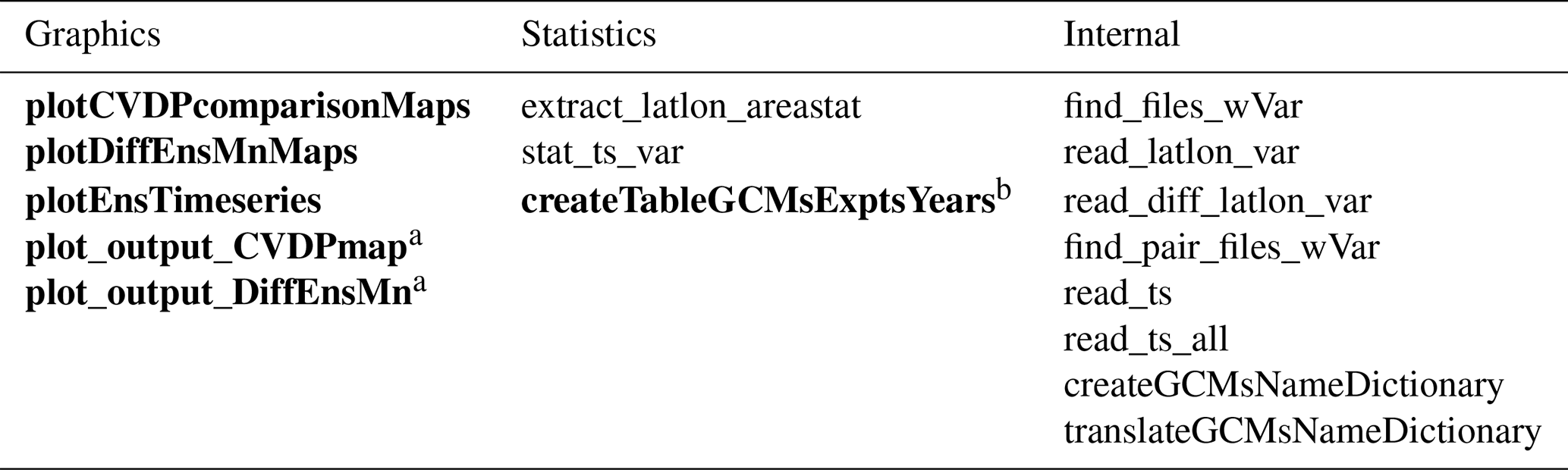
a Returns a netCDF file, as well as an graphic. b Returns a LaTeX-formatted table.
4.2 Python
Similarly to the NCL scripts, most of the analysing and plotting processes in Python have been written into functions, but they are stored in different scripts according to their purposes instead of being written in a single script. Each script was written in notebook format (see Sect. 4.3 for reasons) and named according to its purpose and usage with detailed documentation available in the script. The scripts are built upon the powerful “xarray” package (Hoyer and Hamman, 2017). These scripts all start with a set of five functions to collect the names of available models that have the variable in the experiment and their corresponding directory and filenames and return a dictionary storing this information as “`model_name':`directory/filename'” (hereafter referred to as “target-filename dictionary”). The function identify_ensemble_members requires running find_experiment_ensemble_members.bash in the bin directory to identify available ensemble members (i.e. model names) whose simulations have the target variable in the experiment. Like the NCL scripts, all regridding and multi-model averaging in Python scripts are performed on the fly, and the output can be saved as either a netCDF file or a CSV file based on its type if the user requires. We also have developed a set of plotting schemes in which colours are chosen according to the colour guidelines provided by IPCC WG1 (available at https://github.com/IPCC-WG1/colormaps; last assess: 17 May 2021). Some examples of possible usage are given in Sect. 5.
4.3 Interactive application
One advantage of the Python scripts over the NCL equivalent is their wider user base. Python notebooks allow documentation and outputs to be stored with the scripts. A logical next step is to permit users to interact with the scripts. Attempts using Binder (https://mybinder.org/, last access: 17 March 2022) to create a cloud-computing deployment were found to be underpowered – in part because of the two different coding languages and any data that should be stored along with them. Our solution to this problem is to instead use Docker (https://www.docker.com/, last access: 4 January 2022) to create a containerised application. In this context, the Docker image appears to be a virtual machine storing both required software packages and data, as well as providing a quick and easy method of developing scripts by external users.
Docker images are a hybrid mix of the Linux kernel and bespoke local runtime environment. The Docker image is used to configure and distribute the state of an application. The state of the application in the current context refers to libraries and stored datasets. Dissemination of Docker images via well-known web services such as Docker Hub. The combination of particular software versions (and dependencies) as well as data has been recognised as a useful venue for research reproducibility (Boettiger and Eddelbuettel, 2017; Nüst et al., 2020).
In a host computer equipped with the Docker runtime (widely available for most common operating systems), the Docker image recreates the original system, and the user can access the image either via the command line or, as intended here, using the Jupyter framework via a web browser installed on the host computer. Given that the Docker image may be running on an underpowered computer (e.g. a standard laptop), there are computational limits to what is practical to achieve with this setting. The inclusion of post-processed summary data in the image will however allow users to run analysis on typical laptops. The Docker image is available at https://github.com/pmip4/pmip_p2fvar_analyzer (last access: 10 March 2022) – instructions explaining how to use it are included in the documentation at https://pmip-p2fvar-analyzer.readthedocs.io/ (last access: 4 January 2022). In practice, this requires the user downloading and installing the Docker runtime for their operating system and pointing the Docker runtime to the image on the Internet.
The repository and therefore the interactive image contain a series of summary data of the whole ensemble, as well as a script to download the CVDP output for each individual simulation. The summary data are a series of comma-separated value tables (data_frames in Python terminology), which collect together single pieces of information across each simulation. For example, the file ESGF_doi.csv contains the digital object identifier for each simulation – an important piece of information that should be included in PMIP4 publications to both improve traceability and provide due credit to those having performed the runs. We provide the long-term mean and standard deviation of the interannual time series of area-averaged temperature and precipitation for each region identified by Collins et al. (2013), in the AR5_Regions sub-directory. Statistics of the newly created regional monsoon domains (described in Sect. 3 and plotted in Fig. 7) are included in the monsoon_domains sub-directory. Some metrics that are often computed are tabulated in the common_measures sub-directory – the long-term global mean surface temperature table also includes each model's CMIP generation and equilibrium climate sensitivity (ECS; from Andrews et al., 2012; Zelinka et al., 2020). The temperature changes averaged for 30∘ latitude bands over the land and ocean are included in the tempchange_latbands sub-directory, along with similar tables taken from the supplementary information of PMIP publications. These files form the basis of Fig. 3.2b in IPCC AR6 WG1 (Eyring et al., 2021) and provide the global mean surface temperature in palaeo-periods as estimated from climate models as reported in the “Technical Summary” (Arias et al., 2022) and chap. 2 (Gulev et al., 2021). The CVDP computes many different modes of variability for each simulation (Sect. 3), and the amplitudes of these are tabulated in the climate_modes sub-directory. For indices based on area-averaged sea surface temperature, these are simply the standard deviation of the time series. For modes identified using principal component analysis, the approach of Rehfeld et al. (2020) is adopted and the amplitude is the spatial standard deviation of empirical orthogonal function pattern averaged over same region as the analysis.
By choosing and applying appropriate functions in the scripts, the workflow can produce analyses of temperature, precipitation and monsoon characteristics (and other climatic patterns if required). These analyses can involve just the multi-model mean or individual models and return the outputs as figures (spatial maps, scatter plots, etc.) or data files (as netCDF or CSV) as required. Detailed documentation of the scripts and functions is available elsewhere (such as in the accompanying notebooks) so will not be repeated here. Instead we provide some worked examples of output to help readers get an idea of the possible options. These examples have generally already been featured in PMIP publications or are alluded to in them.

Figure 3Annual mean surface temperature change (∘C) in midHolocene as simulated by individual models that feature Fig. 4 in this work and Fig. 1a in Brierley et al. (2020). Anomalies have been regridded to a 1∘ by 1∘ resolution.
5.1 Plotting spatial patterns
The first example (Fig. 3) is the annual mean temperature difference between midHolocene and piControl, which shows the patterns of temperature change produced by each model in the PMIP4-CMIP6 midHolocene ensemble that features in Brierley et al. (2020). Figure 3 is generated by using the function Calculation_ensemble_change('PMIP4', 'midHolocene', 'tas_spatialmean_ann', 'model') to return a directory containing the regridded annual mean temperature change produced by each model (referred to as tas_data) and the function plot_ensemble_tas(tas_data,'ann') to plot those temperature changes.
The process used to create Fig. 3 has four major steps:
-
Generate target-filename dictionaries for midHolocene and piControl that have the specified variable.
-
Search to see which models occur in both directories, as well as in the prescribed list of PMIP4 model names.
-
Loop through the matching model's midHolocene and piControl simulations individually and then compute the difference (i.e. midHolocene − piControl).
-
Regrid the difference to a 1∘ by 1∘ resolution (in order to easily calculate the multi-model mean) and then store it in the output dictionary named as the model name.
The same function can be used to produce multi-model mean analysis, e.g. the multi-model mean of annual mean surface temperature in the PMIP4-CMIP6 midHolocene ensemble shown in Fig. 4, by entering 'mean' instead of the 'model' used in example 1. This choice requires an additional step: calculate and return the multi-model average and the standard deviation across the ensemble.
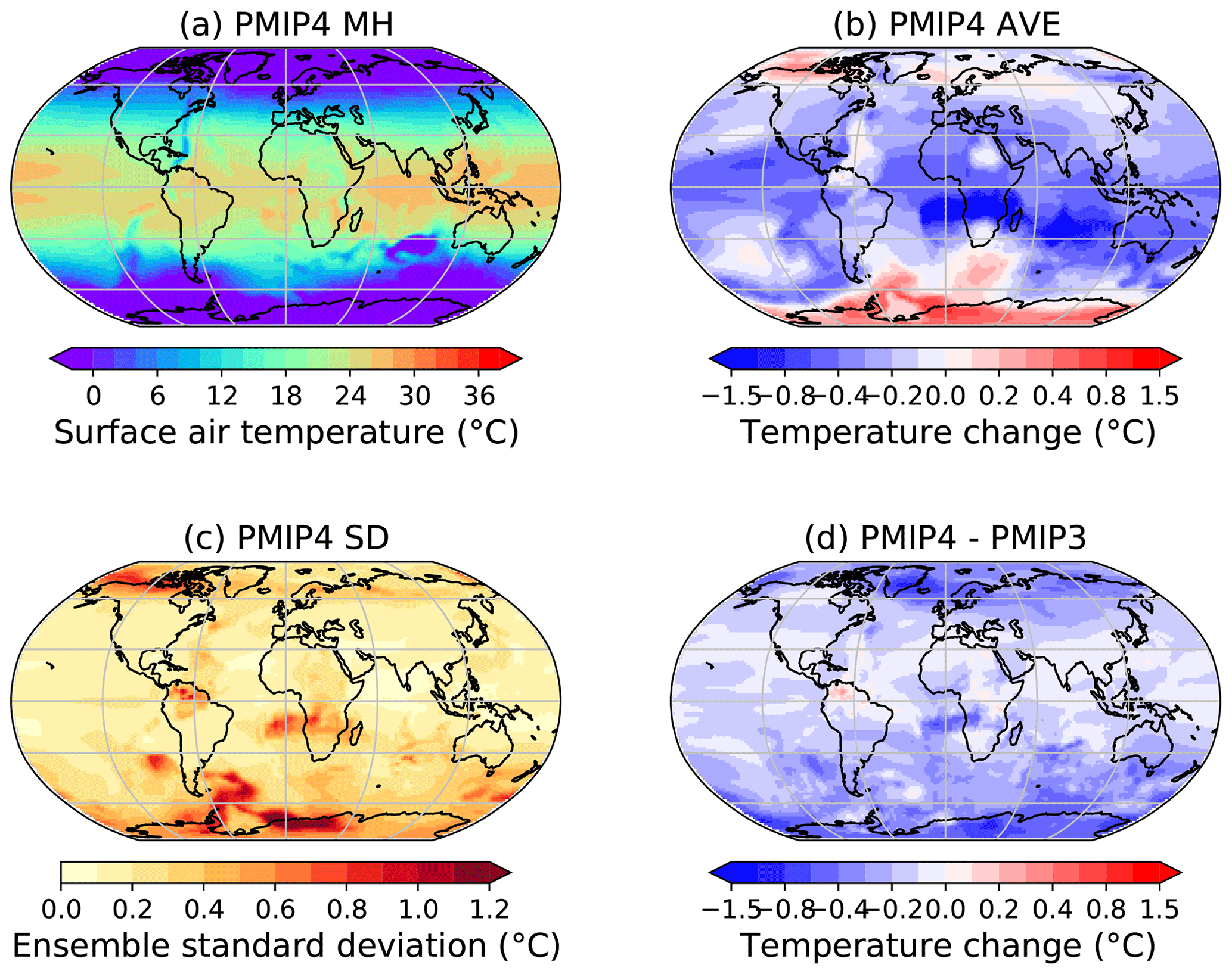
Figure 4Annual mean surface temperature in the midHolocene simulations (∘C). (a) The multi-model mean, Mid-Holocene annual mean surface temperature simulated by PMIP4-CMIP6 midHolocene simulations. (b) The multi-model mean, annual mean temperature changes in PMIP4-CMIP6 (midHolocene − piControl) and (c) the inter-model spread, defined as the across-ensemble standard deviation. (d) The difference in the multi-model mean, annual mean temperature changes between PMIP4-CMIP6 and PMIP3-CMIP5. Panels (a), (b) and (c) are replotted from panels (a), (b) and (e) respectively in Fig. 1 of Brierley et al. (2020).
The NCL programmes do not have the ability to set a flag to determine whether to compute the multi-model mean or individual panels for each ensemble member. Instead they determine the ensemble behaviour depending on the dimension of files containing the requested input variables. If a difference plot (called using plotDiffEnsMnMaps) detects multiple files for each input, then it will compute a multi-model average of the anomalies. Should the second named experiment resolve to only a single file, then the anomaly between each ensemble member and this file will be computed (this functionality was built to compute the multi-model mean of the biases from a single observational dataset). We provide example code (multi-panel_plot.ncl) that was used to create Fig. 7 of Brown et al. (2020). This script also demonstrates two of the supra-resources: CONSISTENCY = True provides stippling to highlight where at least two-thirds of the ensemble members show the same sign of anomaly as the multi-model mean, whilst OVERLAY_CONTROL = True adds contour lines showing the multi-model mean of the variable in the second experiment named (“piControl” in this case).
5.2 Plotting oceanic patterns – the Atlantic meridional overturning circulation (AMOC)
The output files from the CVDP can be used as input for computing multi-mean AMOC changes (midHolocene − piControl) in PMIP4 simulations. The variable called “amoc_mean_ann”, which is analysed with the modified version of the CVDP for individual model simulations, is loaded by Iris for both the Mid-Holocene and piControl ensembles; then all CVDP outputs are regridded on to a 1∘ latitude grid with 61 depth levels between 0–6000 m. This process is achieved through Iris cube's interpolation and regridding schemes called iris.analysis.Linear(). Since models can have different names for their dimension coordinates, basic cube mathematics can not be performed directly. Therefore, only the regridded data in each model are extracted for calculating the differences and averages at this stage. The multi-model mean AMOC change is computed by taking the same steps as in Sect. 5.1. After that, the model-averaged data are put back into one of the regridded models in order to use its dimension coordinates for further plotting. The figure is plotted using “iris.quickplot”, which provides a visualisation for a cube with a title, x and y labels, and a colour bar where appropriate.
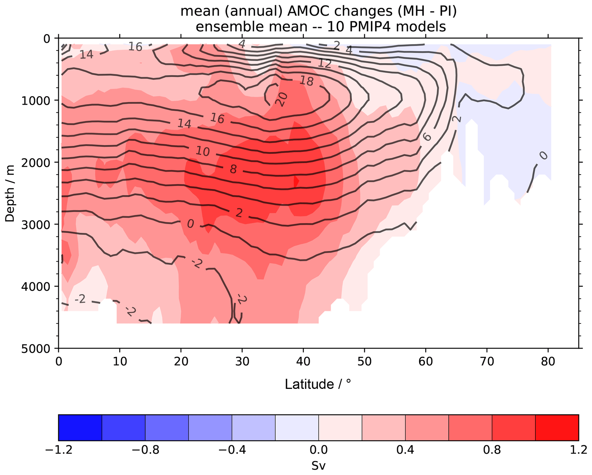
Figure 5Multi-model mean plots for AMOC spatial structure changes between midHolocene and piControl. Eleven PMIP4 models which performed the midHolocene experiment are used for plotting the multi-model means. The overlaid contours (black lines) show AMOC strength in piControl for locating the maximum AMOC.
In addition, the amoc_mean_ann variable derived from the CVDP output files can also be used as an input for generating the AMOC profile for a specific latitude, e.g. 30∘ N. This is helpful when comparing the AMOC strength throughout all depths in different PMIP4 experiments and was used to create the scatter plot of AMOC values shown in Fig. 10 of Brierley et al. (2020).
5.3 Plotting time series
The CVDP can also be used to analyse and generate time series data. Figure 6 gives an example of the analysed results of calendar-adjusted monthly mean sea ice areas (defined as the sea ice fraction multiplied by the area of each grid cell) in the Arctic in the midHolocene and piControl simulations. Lines are coloured following the standard CMIP6 model colour scheme (available at https://github.com/IPCC-WG1/colormaps/blob/master/CMIP6_color.xlsx, last access: 15 May 2021).
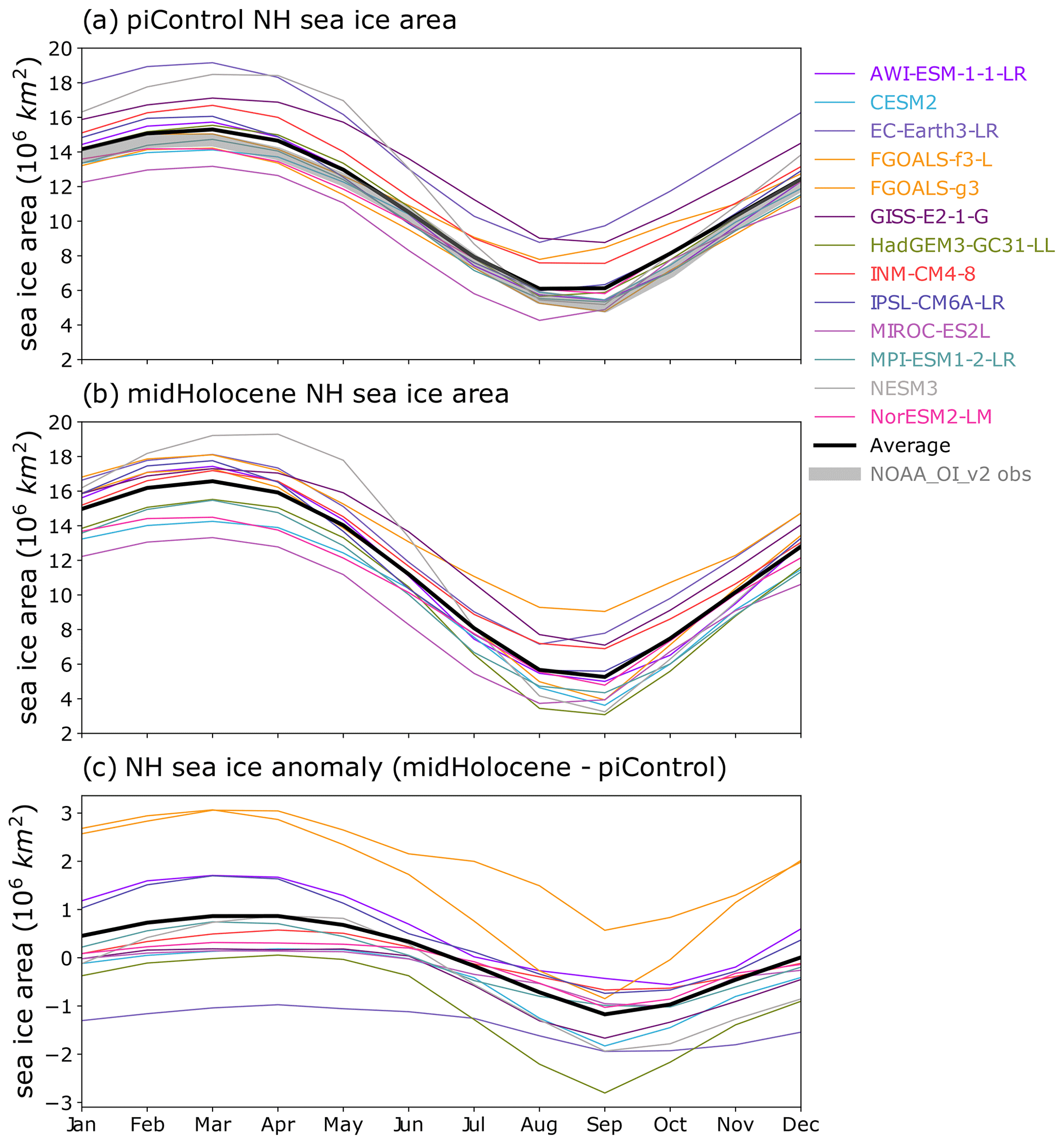
Figure 6Annual cycle of the Arctic sea ice area (106 km2) for (a) piControl, (b) midHolocene and (c) their anomaly (midHolocene − piControl), replotted from Fig. 17 of Otto-Bliesner et al. (2021). The grey line in panel (a) shows the observed monthly mean sea ice areas from the NOAA_OI_v2 dataset for 1982–2001 (Reynolds et al., 2002).
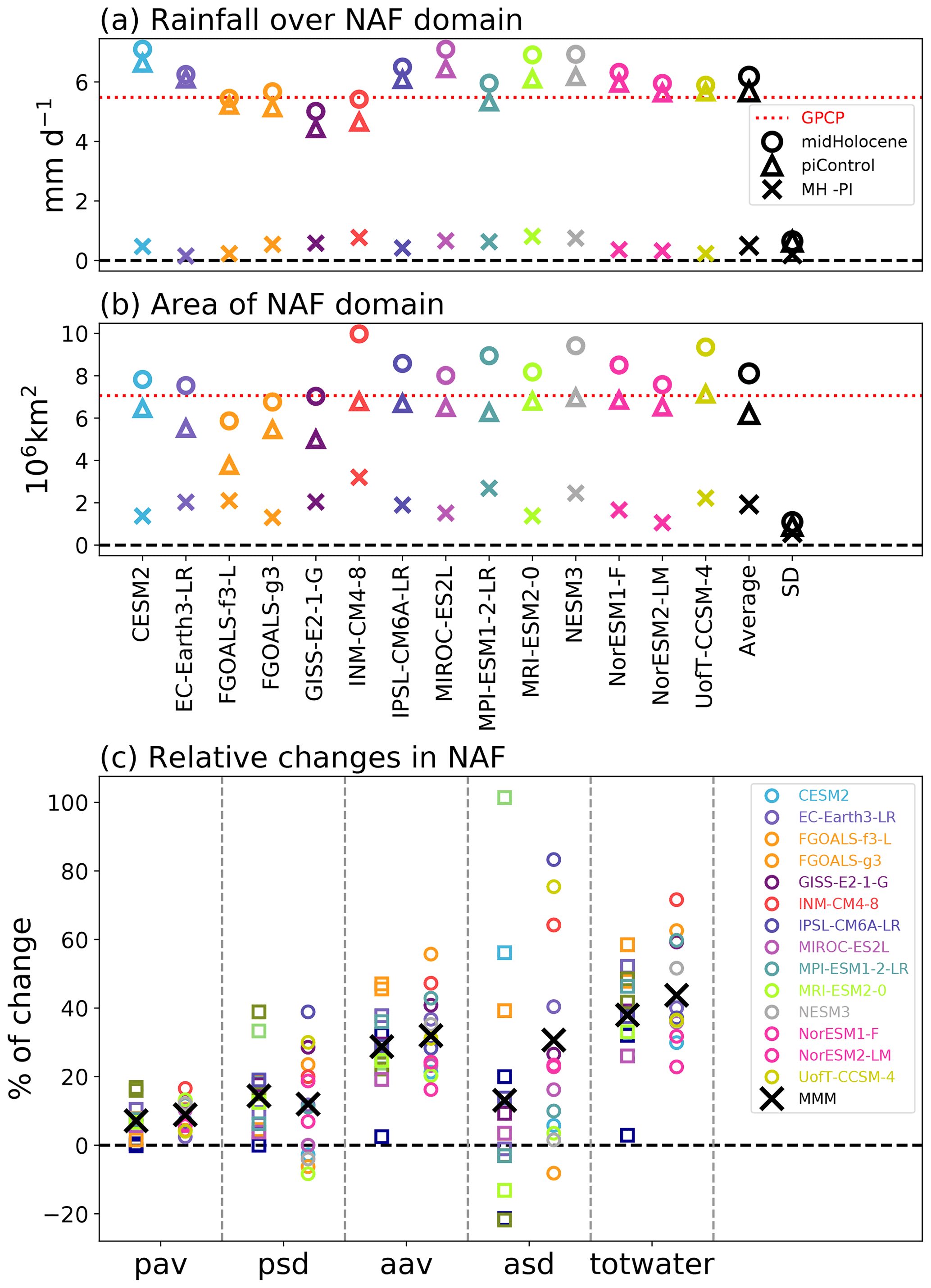
Figure 7Changes in the North African Monsoon (NAF). (a) Area-averaged NAF monsoon summer rain rate (mm d−1) in the midHolocene (circles) and piControl (triangles) simulations and the difference between them (midHolocene − piControl in crosses). (b) The same as panel (a) but for the areal extent of NAF. The dotted red lines in panels (a) and (b) show the corresponding climatology seen in the 1971–2000 GPCP observational dataset (Adler et al., 2003). (c) Relative changes (Brierley et al., 2020) in five different monsoon diagnostics beginning from left in order are the change in area-averaged monsoon summer rain rate (pav), the change in the standard deviation of interannual variability in the area-averaged monsoon summer rain rate (psd), the change in the areal extent of the NAF domain (aav), the change in the standard deviation of interannual variability in the areal extent of the NAF domain (asd) and the percentage change in the total amount of water precipitated in each monsoon season computed as the precipitation rate multiplied by the areal extent (totwater). Colours follow the standard colours for CMIP6 models used in IPCC AR6. If a PMIP3-CMIP5 model (square) is an earlier version of a PMIP4-CMIP6 model, it is coloured the same as the PMIP4-CMIP6 one; otherwise it is coloured dark blue.
5.4 Computing statistics
Our scripts can compute statistics from the output files created by the CVDP. The simplest statistic that might be needed is the length of the data records for a particular variable. The example script generate_model_table.ncl interrogates the directory to extract the number of years available for every simulation containing a variable called nino34 performed under a series of specified experiments. The resulting table can be output either as a spreadsheet (as comma-separated values) or in a format to be directly inputted into a LaTeX file.

Figure 8NAF poleward extension in the PMIP4-CMIP6 midHolocene and lig127k ensembles. (a) The latitude of the poleward boundary of the NAF in the simulations and (b) the northward monsoon extension. The boundary is the latitude where the zonal mean summer (MJJAS) rain rate equals 2 mm d−1 over north Africa (15∘ W–30∘ E).
Given a monthly mean precipitation netCDF file as an input, the CVDP outputs time series of the monsoon rainfall rate (Fig. 7a) and areal extent (Fig. 7b) of each regional monsoon (Sect. 3). Figure 7 is the result of this computation for the North African Monsoon. It uses these time series to compute relative changes in monsoon characteristics in the midHolocene experiment relative to piControl and shows the five available diagnostics (Brierley et al., 2020).
It is also possible to compute areal statistics from the latitude–longitude fields. As part of our modifications to the CVDP, area-weighted average monthly time series for the AR5 regions are now computed for both precipitation and temperature (Sect. 3). To cope with the modification of those regions for AR6 (Iturbide et al., 2020), the area-average precipitation changes shown in Fig. 3.11 of Eyring et al. (2021) are instead computed from the 2D “pr_spatialmean_ann” variable. An alternate approach to look at the poleward extension of the areal extent of the North African Monsoon is to compute the most northerly latitude reached by the monsoon (as in Table S2 of Brierley et al., 2020). Figure 8 gives an example of the North African Monsoon (NAF) expansion in the midHolocene and lig127k ensembles. We define a series of functions to determine the change in latitude where the zonal mean summer (MJJAS) rain rate (stored in the files as “monsoon_summer_rainrate”) equals 2 mm d−1 over north Africa (15∘ W–30∘ E). See the corresponding notebook for details.
The simulations that have been performed for PMIP4-CMIP6 and the large amount of model output available from them are great resources for understanding past climates. The procedure by which this model output is analysed as an ensemble can be time-consuming and involve some methodological decisions. Here we have described the way that our group have chosen to perform our recent analyses (Brierley et al., 2020; Otto-Bliesner et al., 2021; Brierley and Wainer, 2018; Rehfeld et al., 2020; Brown et al., 2020). We document the approach used to obtain and curate PMIP4-CMIP6 simulations, process those outputs via the Climate Variability Diagnostics Package (CVDP), and then continue through to compute ensemble-wide statistics and create ensemble figures. We know from personal experience that replicating the results from published work can often involve reverse engineering the decisions made by researchers during their data processing, and the work presented in this paper removes the need for such effort.
PMIP4 only exists because of the spirit of openness and cooperation within its community, which neatly combines with the IPCC's desire for greater transparency about the figures and data contained within the Sixth Assessment Report. Through documenting our workflow here, we continue in that vein. Hopefully our efforts, such as collation of all the PMIP-related DOIs, make it easier for others to also be transparent in their research.
The main contribution of this work is not the documentation though – rather it is the provision of post-processed files for each PMIP4-CMIP6 simulation alongside scripts to readily convert them into publication-ready figures and tables. The interactive application should further lower the barriers to analysis of palaeoclimate model research. We hope that readers are inspired with ideas of potential analyses that they themselves can perform quickly and easily by using the results of our workflow and scripts as tools to analyse PMIP4-CMIP6 simulations.
All the codes discussed in the above workflow are available from the PMIP4 organisation on GitHub and from Zenodo in different repositories. The original PaleoCalAdjust software is at https://doi.org/10.5281/zenodo.1478824 (Bartlein, 2021), and the operational version discussed in Sect. 2 can be found at https://github.com/pmip4/PaleoCalAdjust (last access: 14 February 2022) and at https://doi.org/10.5281/zenodo.5931062 (Bartlein and Brierley, 2022). The original Climate Variability Diagnostics Package software is at https://github.com/NCAR/CVDP-ncl (last access: 14 February 2022), and the operational version discussed in Sect. 3 can be found at https://github.com/pmip4/CVDP-ncl (last access: 14 February 2022) and at https://doi.org/10.5281/zenodo.5931098 (Phillips and Brierley, 2022). All the scripts discussed in Sect. 4.1 and 4.2 and the examples in Sect. 5 can be found within the combined repository at https://github.com/pmip4/pmip_p2fvar_analyzer (last access: 10 March 2022) and at https://doi.org/10.5281/zenodo.5929684 (Zhao and Brierley, 2022). These scripts, bundled with relevant data files, can be downloaded as a Docker image to allow the user to interact with them (see the documentation in the repository).
The original climate model output is available from the Earth System Grid Federation. Curated directories can be made available on request to c.brierley@ucl.ac.uk or can be found at https://doi.org/10.5281/zenodo.5931086 (Brierley, 2022). A subset of post-processed data is already included in the main repository at https://github.com/pmip4/PMIP_past2future_analyzer (last access: 10 March 2022) and at https://doi.org/10.5281/zenodo.5929684 (Zhao and Brierley, 2022), which includes scripts to download the rest if required.
AZ and CMB devised and wrote the manuscript. AZ wrote all the Python scripts, documentation and the majority of the examples presented. CMB wrote the NCL scripts. ZJ contributed the AMOC example. DO co-wrote the preliminary codes developed for the 2019 workshop at University College London (UCL), where these ideas were first explored. JGD undertook initial work on the Docker deployment and documentation creation. RE was responsible for creating and maintaining the curated ESGF database at UCL during the writing of Brierley et al. (2020) and Otto-Bliesner et al. (2021).
The contact author has declared that neither they nor their co-authors have any competing interests.
Publisher's note: Copernicus Publications remains neutral with regard to jurisdictional claims in published maps and institutional affiliations.
This paper would not be possible without the generosity of the palaeoclimate modelling community in donating their model output. We hope that they can in turn benefit from some of the code and post-processed data that we describe here. The workflow would not exist without the development of packages by Adam Phillips, Jon Fasullo and Patrick Bartlein. We would like to thank all those in the UCL Department of Geography, especially David Thornalley, for their support and encouragement. UCL's Faculty of Social & Historical Sciences kindly funded the 2019 workshop, out of which this research emerged.
This research has been supported by the Natural Environment Research Council (grant no. NE/S009736/1).
This paper was edited by Sophie Valcke and reviewed by Patrick Bartlein and one anonymous referee.
Adler, R. F., Huffman, G. J., Chang, A., Ferraro, R., Xie, P.-P., Janowiak, J., Rudolf, B., Schneider, U., Curtis, S., Bolvin, D., Gruber, A., Susskind, J., Arkin, P., and Nelkin, E.: The version-2 global precipitation climatology project (GPCP) monthly precipitation analysis (1979–present), J. Hydrometeorol., 4, 1147–1167, https://doi.org/10.1175/1525-7541(2003)004<1147:TVGPCP>2.0.CO;2, 2003. a
Andrews, T., Gregory, J. M., Webb, M. J., and Taylor, K. E.: Forcing, feedbacks and climate sensitivity in CMIP5 coupled atmosphere-ocean climate models, Geophys. Res. Lett., 39, L09712, https://doi.org/10.1029/2012GL051607, 2012. a
Arias, P. A., Bellouin, N., Coppola, E., Jones, R. G., Krinner, G., Marotzke, J., Naik, V., Palmer, M. D., Plattner, G.-K., Rogelj, J., Rojas, M., Sillmann, J., Storelvmo, T., Thorne, P. W., Trewin, B., Achuta Rao, K., Adhikary, B., Allan, R. P., Armour, K., Bala, G., Barimalala, R., Berger, S., Canadell, J. G., Cassou, C., Cherchi, A., Collins, W., Collins, W. D., Connors, S. L., Corti, S., Cruz, F., Dentener, F. J., Dereczynski, C., Di Luca, A., Diongue Niang, A., Doblas-Reyes, F. J., Dosio, A., Douville, H., Engelbrecht, F., Eyring, V., Fischer, E., Forster, P., Fox-Kemper, B., Fuglestvedt, J. S., Fyfe, J. C., Gillett, N. P., Goldfarb, L., Gorodetskaya, I., Gutierrez, J. M., Hamdi, R., Hawkins, E., Hewitt, H. T., Hope, P., Islam, A. S., Jones, C., Kaufman, D. S., Kopp, R. E., Kosaka, Y., Kossin, J., Krakovska, S., Lee, J.-Y., Li, J., Mauritsen, T., Maycock, T. K., Meinshausen, M., Min, S.-K., Monteiro, P. M. S., Ngo-Duc, T., Otto, F., Pinto, I., Pirani, A., Raghavan, K., Ranasinghe, R., Ruane, A. C., Ruiz, L., Sallée, J.-B., Samset, B. H., Sathyendranath, S., Seneviratne, S. I., Sörensson, A. A., Szopa, S., Takayabu, I., Treguier, A.-M., van den Hurk, B., Vautard, R., von Schuckmann, K., Zaehle, S., Zhang, X., and Zickfeld, K.: Technical Summary, in: Climate Change 2021: The Physical Science Basis. Contribution of Working Group I to the Sixth Assessment Report of the Intergovernmental Panel on Climate Change, edited by: Masson-Delmotte, V., Zhai, P., Pirani, A., Connors, S. L., Péan, C., Berger, S., Caud, N., Chen, Y., Goldfarb, L., Gomis, M. I., Huang, M., Leitzell, K., Lonnoy, E., Matthews, J., Maycock, T. K., Waterfield, T., Yelekçi, O., Yu, R., and Zhou, B., Cambridge University Press, in press, 2022. a
Balaji, V., Taylor, K. E., Juckes, M., Lawrence, B. N., Durack, P. J., Lautenschlager, M., Blanton, C., Cinquini, L., Denvil, S., Elkington, M., Guglielmo, F., Guilyardi, E., Hassell, D., Kharin, S., Kindermann, S., Nikonov, S., Radhakrishnan, A., Stockhause, M., Weigel, T., and Williams, D.: Requirements for a global data infrastructure in support of CMIP6, Geosci. Model Dev., 11, 3659–3680, https://doi.org/10.5194/gmd-11-3659-2018, 2018. a
Bartlein, P.: pjbartlein/PaleoCalAdjust: (v1.1), Zenodo [code], https://doi.org/10.5281/zenodo.1478824, 2021. a
Bartlein, P. and Brierley, C.: pmip4/PaleoCalAdjust: Publishing revisions associated with Zhao et al. manuscript (v1.0.Zhaoetal), Zenodo [code], https://doi.org/10.5281/zenodo.5931062, 2022. a
Bartlein, P. J. and Shafer, S. L.: Paleo calendar-effect adjustments in time-slice and transient climate-model simulations (PaleoCalAdjust v1.0): impact and strategies for data analysis, Geosci. Model Dev., 12, 3889–3913, https://doi.org/10.5194/gmd-12-3889-2019, 2019. a, b
Bartlein, P. J., Harrison, S., Brewer, S., Connor, S., Davis, B., Gajewski, K., Guiot, J., Harrison-Prentice, T., Henderson, A., and Peyron, O.: Pollen-based continental climate reconstructions at 6 and 21 ka: a global synthesis, Clim. Dynam., 37, 775–802, https://doi.org/10.1007/s00382-010-0904-1, 2011. a
Boettiger, C. and Eddelbuettel, D.: An Introduction to Rocker: Docker Containers for R, The R Journal, 9, 527–536, https://doi.org/10.32614/RJ-2017-065, 2017. a
Braconnot, P., Harrison, S. P., Kageyama, M., Bartlein, P. J., Masson-Delmotte, V., Abe-Ouchi, A., Otto-Bliesner, B., and Zhao, Y.: Evaluation of climate models using palaeoclimatic data, Nat. Clim. Change, 2, 417–424, https://doi.org/10.1038/nclimate1456, 2012. a
Braconnot, P., Zhu, D., Marti, O., and Servonnat, J.: Strengths and challenges for transient Mid- to Late Holocene simulations with dynamical vegetation, Clim. Past, 15, 997–1024, https://doi.org/10.5194/cp-15-997-2019, 2019. a
Brierley, C.: pmip4/UCL_curated_ESGF_replica: Publishing status associated with Zhao et al. manuscript (Version v1), Zenodo [code], https://doi.org/10.5281/zenodo.5931086, 2022. a
Brierley, C. and Wainer, I.: Inter-annual variability in the tropical Atlantic from the Last Glacial Maximum into future climate projections simulated by CMIP5/PMIP3, Clim. Past, 14, 1377–1390, https://doi.org/10.5194/cp-14-1377-2018, 2018. a, b, c, d, e, f
Brierley, C. and Zhao, A.: PMIP_for_AR6_Interactive_Atlas, GitHub, https://github.com/chrisbrierley/PMIP_for_AR6_Interactive_Atlas, last access: 12 July 2021. a, b
Brierley, C. M., Zhao, A., Harrison, S. P., Braconnot, P., Williams, C. J. R., Thornalley, D. J. R., Shi, X., Peterschmitt, J.-Y., Ohgaito, R., Kaufman, D. S., Kageyama, M., Hargreaves, J. C., Erb, M. P., Emile-Geay, J., D'Agostino, R., Chandan, D., Carré, M., Bartlein, P. J., Zheng, W., Zhang, Z., Zhang, Q., Yang, H., Volodin, E. M., Tomas, R. A., Routson, C., Peltier, W. R., Otto-Bliesner, B., Morozova, P. A., McKay, N. P., Lohmann, G., Legrande, A. N., Guo, C., Cao, J., Brady, E., Annan, J. D., and Abe-Ouchi, A.: Large-scale features and evaluation of the PMIP4-CMIP6 midHolocene simulations, Clim. Past, 16, 1847–1872, https://doi.org/10.5194/cp-16-1847-2020, 2020. a, b, c, d, e, f, g, h, i, j, k, l, m, n, o, p
Brown, J. R., Brierley, C. M., An, S.-I., Guarino, M.-V., Stevenson, S., Williams, C. J. R., Zhang, Q., Zhao, A., Abe-Ouchi, A., Braconnot, P., Brady, E. C., Chandan, D., D'Agostino, R., Guo, C., LeGrande, A. N., Lohmann, G., Morozova, P. A., Ohgaito, R., O'ishi, R., Otto-Bliesner, B. L., Peltier, W. R., Shi, X., Sime, L., Volodin, E. M., Zhang, Z., and Zheng, W.: Comparison of past and future simulations of ENSO in CMIP5/PMIP3 and CMIP6/PMIP4 models, Clim. Past, 16, 1777–1805, https://doi.org/10.5194/cp-16-1777-2020, 2020. a, b, c, d, e
Christensen, J., Krishna Kumar, K., Aldrian, E., An, S.-I., Cavalcanti, I., de Castro, M., Dong, W.and Goswami, P., Hall, A., Kanyanga, J., Kitoh, A., Kossin, J., Lau, N.-C., Renwick, J., Stephenson, D., Xie, S.-P., and Zhou, T.: Climate phenomena and their relevance for future regional climate change, in: Climate change 2013: the physical science basis. Contribution of Working Group I to the Fifth Assessment Report of the Intergovernmental Panel on Climate Change, edited by: Stocker, T., Qin, D., Plattner, G.-K., Tignor, M., Allen, S., Boschung, J., Nauels, A., Xia, Y., Bex, V., and Midgley, P., 1217–1308, Cambridge University Press, Cambridge, United Kingdom and New York, NY, USA, 2013. a, b
Collins, M., Knutti, R., Arblaster, J., Dufresne, J.-L., Fichefet, T., Friedlingstein, P., Gao, X., Gutowski, W. J., Johns, T., Krinner, G., Shongwe, M., Tebaldi, C., Weaver, A., and Wehner, M.: Long-term climate change: projections, commitments and irreversibility, in: Climate Change 2013-The Physical Science Basis: Contribution of Working Group I to the Fifth Assessment Report of the Intergovernmental Panel on Climate Change, edited by: Stocker, T., Qin, D., Plattner, G.-K., Tignor, M., Allen, S., Boschung, J., Nauels, A., Xia, Y., Bex, V., and Midgley, P., 1029–1136, Cambridge University Press, Cambridge, United Kingdom and New York, NY, USA, 2013. a, b
Danabasoglu, G., Yeager, S. G., Kwon, Y.-O., Tribbia, J. J., Phillips, A. S., and Hurrell, J. W.: Variability of the Atlantic meridional overturning circulation in CCSM4, J. Climate, 25, 5153–5172, 2012. a
Douville, H., Raghavan, K., Renwick, J., Allan, R. P., Arias, P. A., Barlow, M., Cerezo-Mota, R., Cherchi, A., Gan, T. Y., Gergis, J., Jiang, D., Khan, A., Pokam Mba, W., Rosenfeld, D., Tierney, J., and Zolina, O.: Water Cycle Changes, in: Climate Change 2021: The Physical Science Basis. Contribution of Working Group I to the Sixth Assessment Report of the Intergovernmental Panel on Climate Change, edited by: Masson-Delmotte, V., Zhai, P., Pirani, A., Connors, S. L., Péan, C., Berger, S., Caud, N., Chen, Y., Goldfarb, L., Gomis, M. I., Huang, M., Leitzell, K., Lonnoy, E., Matthews, J., Maycock, T. K., Waterfield, T., Yelekçi, O., Yu, R., and Zhou, B., Cambridge University Press, in press, 2022. a, b
Eyring, V., Bony, S., Meehl, G. A., Senior, C. A., Stevens, B., Stouffer, R. J., and Taylor, K. E.: Overview of the Coupled Model Intercomparison Project Phase 6 (CMIP6) experimental design and organization, Geosci. Model Dev., 9, 1937–1958, https://doi.org/10.5194/gmd-9-1937-2016, 2016. a, b, c
Eyring, V., Gillett, N. P., Achuta Rao, K. M., Barimalala, R., Barreiro Parrillo, M., Bellouin, N., Cassou, C., Durack, P. J., Kosaka, Y., McGregor, S., Min, S., Morgenstern, O., and Sun, Y.: Human Influence on the Climate System, in: Climate Change 2021: The Physical Science Basis. Contribution of Working Group I to the Sixth Assessment Report of the Intergovernmental Panel on Climate Change, edited by: Masson-Delmotte, V., Zhai, P., Pirani, A., Connors, S. L., Péan, C., Berger, S., Caud, N., Chen, Y., Goldfarb, L., Gomis, M. I., Huang, M., Leitzell, K., Lonnoy, E., Matthews, J., Maycock, T. K., Waterfield, T., Yelekçi, O., Yu, R, and Zhou, B., Cambridge University Press, in press, 2021. a, b, c, d, e, f, g
Fasullo, J. T., Phillips, A., and Deser, C.: Evaluation of leading modes of climate variability in the CMIP archives, J. Climate, 33, 5527–5545, https://doi.org/10.1175/JCLI-D-19-1024.1, 2020. a
Fox-Kemper, B., Hewitt, H. T., Xiao, C., Aðalgeirsdóttir, G., Drijfhout, S. S., Edwards, T. L., Golledge, N. R., Hemer, M., Kopp, R. E., Krinner, G., Mix, A., Notz, D., Nowicki, S., Nurhati, I. S., Ruiz, L., Sallée, J.-B., Slangen, A. B. A., and Yu, Y.: Ocean, Cryosphere and Sea Level Change, in: Climate Change 2021: The Physical Science Basis. Contribution of Working Group I to the Sixth Assessment Report of the Intergovernmental Panel on Climate Change, edited by: Masson-Delmotte, V., Zhai, P., Pirani, A., Connors, S. L., Péan, C., Berger, S., Caud, N., Chen, Y., Goldfarb, L., Gomis, M. I., Huang, M., Leitzell, K., Lonnoy, E., Matthews, J., Maycock, T. K., Waterfield, T., Yelekçi, O., Yu, R., and Zhou, B., Cambridge University Press, in press, 2021. a
Gulev, S. K., Thorne, P., Ahn, J., Dentener, F., Domingues, C., Gerland, S., Gong, D., Kaufman, D., Nnamchi, H., Quaas, J., Rivera, J., Sathyendranath, S., Smith, S., Trewin, B., von Shuckmann, K., and Vose, R.: Changing State of the Climate System, in: Climate Change 2021: The Physical Science Basis. Contribution of Working Group I to the Sixth Assessment Report of the Intergovernmental Panel on Climate Change, edited by: Masson-Delmotte, V., Zhai, P., Pirani, A., Connors, S. L., Péan, C., Berger, S., Caud, N., Chen, Y., Goldfarb, L., Gomis, M. I., Huang, M., Leitzell, K., Lonnoy, E., Matthews, J., Maycock, T. K., Waterfield, T., Yelekçi, O., Yu, R., and Zhou, B., Cambridge University Press, in press, 2021. a, b, c
Gutiérrez, J. M., Iturbide, M., Alvarez, E. C., Diez-Sierra, J., Bedia, J., Manzanas, R., no Medina, J. B., Hauser, M., García-Díez, M., Ozge Yelecki, Felice, M. D., and Trenham, C.: PMIP4-midHolocene, GitHub, https://github.com/IPCC-WG1/Atlas, last access: 12 July 2021. a
Gutiérrez, J. M., Jones, R. G., Narisma, G. T., Alves, L. M., Amjad, M., Gorodetskaya, I. V., Grose, M., Klutse, N. A. B., Krakovska, S., Li, J., Martínez-Castro, D., Mearns, L. O., Mernild, S. H., Ngo-Duc, T., van den Hurk, B., and Yoon, J.-H.: Atlas, in: Climate Change 2021: The Physical Science Basis. Contribution of Working Group I to the Sixth Assessment Report of the Intergovernmental Panel on Climate Change, edited by: Masson-Delmotte, V., Zhai, P., Pirani, A., Connors, S. L., Péan, C., Berger, S., Caud, N., Chen, Y., Goldfarb, L., Gomis, M. I., Huang, M., Leitzell, K., Lonnoy, E., Matthews, J., Maycock, T. K., Waterfield, T., Yelekçi, O., Yu, R., and Zhou, B., Cambridge University Press, in press, 2022. a, b, c
Harrison, S., Bartlein, P., Brewer, S., Prentice, I., Boyd, M., Hessler, I., Holmgren, K., Izumi, K., and Willis, K.: Climate model benchmarking with glacial and mid-Holocene climates, Clim. Dynam., 43, 671–688, https://doi.org/10.1007/s00382-013-1922-6, 2014. a
Harrison, S. P., Bartlein, P., Izumi, K., Li, G., Annan, J., Hargreaves, J., Braconnot, P., and Kageyama, M.: Evaluation of CMIP5 palaeo-simulations to improve climate projections, Nat. Clim. Change, 5, 735–743, https://doi.org/10.1038/nclimate2649, 2015. a
Haywood, A. M., Tindall, J. C., Dowsett, H. J., Dolan, A. M., Foley, K. M., Hunter, S. J., Hill, D. J., Chan, W.-L., Abe-Ouchi, A., Stepanek, C., Lohmann, G., Chandan, D., Peltier, W. R., Tan, N., Contoux, C., Ramstein, G., Li, X., Zhang, Z., Guo, C., Nisancioglu, K. H., Zhang, Q., Li, Q., Kamae, Y., Chandler, M. A., Sohl, L. E., Otto-Bliesner, B. L., Feng, R., Brady, E. C., von der Heydt, A. S., Baatsen, M. L. J., and Lunt, D. J.: The Pliocene Model Intercomparison Project Phase 2: large-scale climate features and climate sensitivity, Clim. Past, 16, 2095–2123, https://doi.org/10.5194/cp-16-2095-2020, 2020. a
Hoyer, S. and Hamman, J.: xarray: N-D labeled arrays and datasets in Python, J. Open Res. Softw., 5, 10, https://doi.org/10.5334/jors.148, 2017. a
IPCC: Annex V: Monsoons, in: Climate Change 2021: The Physical Science Basis. Contribution of Working Group I to the Sixth Assessment Report of the Intergovernmental Panel on Climate Change, edited by: Masson-Delmotte, V., Zhai, P., Pirani, A., Connors, S. L., Péan, C., Berger, S., Caud, N., Chen, Y., Goldfarb, L., Gomis, M. I., Huang, M., Leitzell, K., Lonnoy, E., Matthews, J., Maycock, T. K., Waterfield, T., Yelekçi, O., Yu, R., and Zhou, B., Cambridge University Press, 2021. a, b
Iturbide, M., Gutiérrez, J. M., Alves, L. M., Bedia, J., Cerezo-Mota, R., Cimadevilla, E., Cofiño, A. S., Di Luca, A., Faria, S. H., Gorodetskaya, I. V., Hauser, M., Herrera, S., Hennessy, K., Hewitt, H. T., Jones, R. G., Krakovska, S., Manzanas, R., Martínez-Castro, D., Narisma, G. T., Nurhati, I. S., Pinto, I., Seneviratne, S. I., van den Hurk, B., and Vera, C. S.: An update of IPCC climate reference regions for subcontinental analysis of climate model data: definition and aggregated datasets, Earth Syst. Sci. Data, 12, 2959–2970, https://doi.org/10.5194/essd-12-2959-2020, 2020. a
Juckes, M., Taylor, K. E., Durack, P. J., Lawrence, B., Mizielinski, M. S., Pamment, A., Peterschmitt, J.-Y., Rixen, M., and Sénési, S.: The CMIP6 Data Request (DREQ, version 01.00.31), Geosci. Model Dev., 13, 201–224, https://doi.org/10.5194/gmd-13-201-2020, 2020. a
Kageyama, M., Braconnot, P., Harrison, S. P., Haywood, A. M., Jungclaus, J. H., Otto-Bliesner, B. L., Peterschmitt, J.-Y., Abe-Ouchi, A., Albani, S., Bartlein, P. J., Brierley, C., Crucifix, M., Dolan, A., Fernandez-Donado, L., Fischer, H., Hopcroft, P. O., Ivanovic, R. F., Lambert, F., Lunt, D. J., Mahowald, N. M., Peltier, W. R., Phipps, S. J., Roche, D. M., Schmidt, G. A., Tarasov, L., Valdes, P. J., Zhang, Q., and Zhou, T.: The PMIP4 contribution to CMIP6 – Part 1: Overview and over-arching analysis plan, Geosci. Model Dev., 11, 1033–1057, https://doi.org/10.5194/gmd-11-1033-2018, 2018. a, b, c
Kageyama, M., Harrison, S. P., Kapsch, M.-L., Lofverstrom, M., Lora, J. M., Mikolajewicz, U., Sherriff-Tadano, S., Vadsaria, T., Abe-Ouchi, A., Bouttes, N., Chandan, D., Gregoire, L. J., Ivanovic, R. F., Izumi, K., LeGrande, A. N., Lhardy, F., Lohmann, G., Morozova, P. A., Ohgaito, R., Paul, A., Peltier, W. R., Poulsen, C. J., Quiquet, A., Roche, D. M., Shi, X., Tierney, J. E., Valdes, P. J., Volodin, E., and Zhu, J.: The PMIP4 Last Glacial Maximum experiments: preliminary results and comparison with the PMIP3 simulations, Clim. Past, 17, 1065–1089, https://doi.org/10.5194/cp-17-1065-2021, 2021. a
Kitoh, A., Endo, H., Krishna Kumar, K., Cavalcanti, I. F. A., Goswami, P., and Zhou, T.: Monsoons in a changing world: A regional perspective in a global context, J. Geophys. Res.-Atmos., 118, 3053–3065, https://doi.org/10.1002/jgrd.50258, 2013. a
Nüst, D., Sochat, V., Marwick, B., Eglen, S. J., Head, T., Hirst, T., and Evans, B. D.: Ten simple rules for writing Dockerfiles for reproducible data science, PLOS Comput. Biol., 16, 1–24, https://doi.org/10.1371/journal.pcbi.1008316, 2020. a
Otto-Bliesner, B. L., Brady, E. C., Fasullo, J., Jahn, A., Landrum, L., Stevenson, S., Rosenbloom, N., Mai, A., and Strand, G.: Climate variability and change since 850 CE: An ensemble approach with the Community Earth System Model, B. Am. Meteorol. Soc., 97, 735–754, 2016. a
Otto-Bliesner, B. L., Braconnot, P., Harrison, S. P., Lunt, D. J., Abe-Ouchi, A., Albani, S., Bartlein, P. J., Capron, E., Carlson, A. E., Dutton, A., Fischer, H., Goelzer, H., Govin, A., Haywood, A., Joos, F., LeGrande, A. N., Lipscomb, W. H., Lohmann, G., Mahowald, N., Nehrbass-Ahles, C., Pausata, F. S. R., Peterschmitt, J.-Y., Phipps, S. J., Renssen, H., and Zhang, Q.: The PMIP4 contribution to CMIP6 – Part 2: Two interglacials, scientific objective and experimental design for Holocene and Last Interglacial simulations, Geosci. Model Dev., 10, 3979–4003, https://doi.org/10.5194/gmd-10-3979-2017, 2017. a
Otto-Bliesner, B. L., Brady, E. C., Zhao, A., Brierley, C. M., Axford, Y., Capron, E., Govin, A., Hoffman, J. S., Isaacs, E., Kageyama, M., Scussolini, P., Tzedakis, P. C., Williams, C. J. R., Wolff, E., Abe-Ouchi, A., Braconnot, P., Ramos Buarque, S., Cao, J., de Vernal, A., Guarino, M. V., Guo, C., LeGrande, A. N., Lohmann, G., Meissner, K. J., Menviel, L., Morozova, P. A., Nisancioglu, K. H., O'ishi, R., Salas y Mélia, D., Shi, X., Sicard, M., Sime, L., Stepanek, C., Tomas, R., Volodin, E., Yeung, N. K. H., Zhang, Q., Zhang, Z., and Zheng, W.: Large-scale features of Last Interglacial climate: results from evaluating the lig127k simulations for the Coupled Model Intercomparison Project (CMIP6)–Paleoclimate Modeling Intercomparison Project (PMIP4), Clim. Past, 17, 63–94, https://doi.org/10.5194/cp-17-63-2021, 2021. a, b, c, d, e, f, g, h
Phillips, A. and Brierley, C.: pmip4/CVDP-ncl: Publishing revisions associated with Zhao et al. manuscript (v.5.2.pmip4), Zenodo [code], https://doi.org/10.5281/zenodo.5931098, 2022. a
Phillips, A. S., Deser, C., and Fasullo, J.: Evaluating modes of variability in climate models, Eos, Transactions American Geophysical Union, 95, 453–455, https://doi.org/10.1002/2014EO490002, 2014. a
Pollard, D. and Reusch, D. B.: A calendar conversion method for monthly mean paleoclimate model output with orbital forcing, J. Geophys. Res.-Atmos., 107, 4615–ACL3–7, https://doi.org/10.1029/2002JD002126, 2002. a
Rehfeld, K., Hébert, R., Lora, J. M., Lofverstrom, M., and Brierley, C. M.: Variability of surface climate in simulations of past and future, Earth Syst. Dynam., 11, 447–468, https://doi.org/10.5194/esd-11-447-2020, 2020. a, b, c, d, e
Reynolds, R. W., Rayner, N. A., Smith, T. M., Stokes, D. C., and Wang, W.: An Improved In Situ and Satellite SST Analysis for Climate, J. Climate, 15, 1609–1625, https://doi.org/10.1175/1520-0442(2002)015<1609:AIISAS>2.0.CO;2, 2002. a
Schmidt, G. A., Annan, J. D., Bartlein, P. J., Cook, B. I., Guilyardi, E., Hargreaves, J. C., Harrison, S. P., Kageyama, M., LeGrande, A. N., Konecky, B., Lovejoy, S., Mann, M. E., Masson-Delmotte, V., Risi, C., Thompson, D., Timmermann, A., Tremblay, L.-B., and Yiou, P.: Using palaeo-climate comparisons to constrain future projections in CMIP5, Clim. Past, 10, 221–250, https://doi.org/10.5194/cp-10-221-2014, 2014. a
Wang, B. and Ding, Q.: Global monsoon: Dominant mode of annual variation in the tropics, Dynam. Atmos. Oceans, 44, 165–183, https://doi.org/10.1016/j.dynatmoce.2007.05.002, 2008. a
Wang, B., Kim, H.-J., Kikuchi, K., and Kitoh, A.: Diagnostic metrics for evaluation of annual and diurnal cycles, Clim. Dynam., 37, 941–955, https://doi.org/10.1007/s00382-010-0877-0, 2011. a
Wang, P. X., Wang, B., Cheng, H., Fasullo, J., Guo, Z. T., Kiefer, T., and Liu, Z. Y.: The global monsoon across timescales: coherent variability of regional monsoons, Clim. Past, 10, 2007–2052, https://doi.org/10.5194/cp-10-2007-2014, 2014. a
Zelinka, M. D., Myers, T. A., McCoy, D. T., Po-Chedley, S., Caldwell, P. M., Ceppi, P., Klein, S. A., and Taylor, K. E.: Causes of higher climate sensitivity in CMIP6 models, Geophys. Res. Lett., 47, e2019GL085782, https://doi.org/10.1029/2019GL085782, 2020. a
Zender, C. S.: Analysis of self-describing gridded geoscience data with netCDF Operators (NCO), Environ. Model. Softw., 23, 1338–1342, 2008. a
Zhao, A. and Brierley, C.: pmip4/pmip_p2fvar_analyzer: Incorporating revisions associated with Zhao et al. manuscript (v1.1), Zenodo [code], https://doi.org/10.5281/zenodo.5929684, 2022. a, b