ShellChron 0.4.0: a new tool for constructing chronologies in accretionary carbonate archives from stable oxygen isotope profiles

This work presents ShellChron, a new model for generating accurate internal age models for high-resolution paleoclimate archives, such as corals, mollusk shells, and speleothems. Reliable sub-annual age models form the backbone of high-resolution paleoclimate studies. In the absence of independent sub-annual growth markers in many of these archives, the most reliable method for determining the age of samples is through age modeling based on stable oxygen isotope or other seasonally controlled proxy records. ShellChron expands on previous solutions to the age model problem by fitting a combination of a growth rate and temperature sinusoid to model seasonal variability in the proxy record in a sliding window approach. This new approach creates smoother, more precise age–distance relationships for multi-annual proxy records with the added benefit of allowing assessment of the uncertainty in the modeled age. The modular script of ShellChron allows the model to be tailored to specific archives, without being limited to oxygen isotope proxy records or carbonate archives, with high flexibility in assigning the relationship between the input proxy and the seasonal cycle. The performance of ShellChron in terms of accuracy and computation time is tested on a set of virtual seasonality records and real coral, mollusk, and speleothem archives. The result shows that several key improvements in comparison to previous age model routines enhance the accuracy of ShellChron on multi-annual records while limiting its processing time. The current full working version of ShellChron enables the user to model the age of 10-year-long high-resolution (16 samples yr⁻¹) carbonate records with monthly accuracy within 1 h of computation time on a personal computer. The model is freely accessible on the CRAN database and GitHub. Members of the community are invited to contribute by adapting the model code to suit their research topics and encouraged to cite the original work of Judd et al. (2018) alongside this work when using ShellChron in future studies.

1 Introduction

Fast-growing carbonate archives, such as coral skeletons, mollusk shells, and speleothems, contain a wealth of information about past and present climate and environment (e.g., Urban et al., 2000; Wang et al., 2001; Steuber et al., 2005; Butler et al., 2013). Recent advances in analytical techniques have improved our ability to extract this information and obtain records of the conditions under which these carbonates precipitated at high temporal resolutions, often beyond the annual scale (Treble et al., 2007; Saenger et al., 2017; Vansteenberge et al., 2020; de Winter et al., 2020a; Ivany and Judd, 2022). Key to the interpretation of such records is the development of reliable chemical or physical proxies for climate and environmental conditions which can be measured on a sufficiently fine scale to allow variability to be reconstructed at the desired time resolution. Examples of suitable proxies include observations of variability in carbonate fabric and microstructure as well as in (trace) elemental and isotopic composition (Frisia et al., 2000; Lough, 2010; Ullmann et al., 2010; Schöne et al., 2011; Ullmann et al., 2013; Van Rampelbergh et al., 2014; de Winter et al., 2017). The unique preservation potential of carbonates in comparison with archives of climate variability at similar time resolutions, such as tree ring records and ice cores, now allows us to recover information about the climate and environment of the geological past from these proxies on the (sub-)seasonal scale (Ivany and Runnegar, 2010; Ullmann and Korte, 2015; Vansteenberge et al., 2016; de Winter et al., 2018, 2020b, c; Mohr et al., 2020). The importance of this development cannot be overstated because variability at high (daily and seasonal) resolution constitutes the most significant component of climate variability (Mitchell, 1976; Huybers and Curry, 2006; Zhu et al., 2019; von der Heydt et al., 2021). Accurate reconstructions of this type of variability are therefore fundamental to our understanding of Earth's climate system and critical for projecting its behavior in the future under anthropogenic global warming conditions (IPCC, 2021).

A reliable age model is crucial for the interpretation of high-resolution carbonate records. An age model is defined as a set of rules or markers that allows the translation of the location of a measurement or observation on the archive to the time at which the carbonate was precipitated. This translation is required for aligning records from multiple proxies or archives on a common time axis. Age alignment enables data to be intercomparable and to be interpreted in the context of processes playing a role at similar timescales. Age models are based on knowledge about the growth or accretion rate of the archive through time. Many high-resolution carbonate archives contain growth markers on which age models can be based (e.g., Jones, 1983; Le Tissier et al., 1994; Verheyden et al., 2006). These are especially valuable in some mollusk species, in which growth lines demarcate annual, daily, or even tidal cycles (e.g., Arctica islandica, Schöne et al., 2005; Pecten maximus, Chauvaud et al., 2005; and Cerastoderma edule, Mahé et al., 2010). However, in many mollusk species and most carbonate archives, such independent growth indicators are absent or too infrequent to (relatively) date high-resolution measurements (Judd et al., 2018; Huyghe et al., 2019). In such cases, age models need to be based on alternative indicators.

The oxygen isotope composition of carbonates (δ¹⁸O_c) is closely dependent on the isotopic composition of the fluid (δ¹⁸O_w) and the temperature at which the carbonate is precipitated (Urey, 1948; McCrea, 1950; Epstein et al., 1953). In most natural surface environments, either one or both factors is strongly dependent on the seasonal cycle, with one generally being dominant over the other. This causes carbonates precipitated in these environments to display strong quasi-sinusoidal variations in δ¹⁸O_c that record the seasonal cycle (e.g., Dunbar and Wellington, 1981; Jones and Quitmyer, 1996; Baldini et al., 2008). Examples of this behavior include seasonal cyclicity in sea surface temperatures recorded in the δ¹⁸O_c of corals and mollusks and seasonal cyclicity in the δ¹⁸O_w of precipitation recorded in speleothems (Dunbar and Wellington, 1981; Schöne et al., 2005; Van Rampelbergh et al., 2014). This relationship is challenged in tropical latitudes, where temperature seasonality is restricted. However, in some tropical archives, the annual cycle of δ¹⁸O_w in precipitation still allows the annual cycle to be resolved from δ¹⁸O records (e.g., Evans and Schrag, 2004). These properties make δ¹⁸O_c one of the most highly sought-after proxies for climate variability, and high-resolution δ¹⁸O_c records are abundant in the paleoclimate literature (e.g., Lachniet, 2009; Lough, 2010; Schöne and Gillikin, 2013, and references therein).

The close relationship between δ¹⁸O_c records and the seasonal cycle can also be exploited to estimate variability in growth rate of the archive. This property of δ¹⁸O_c curves has been recognized by previous authors, and attempts have been made to quantify intra-annual growth rates from the shape of δ¹⁸O_c profiles (Wilkinson and Ivany, 2002; Goodwin et al., 2003; De Ridder et al., 2006; Goodwin et al., 2009; De Brauwere et al., 2009; Müller et al., 2015; Judd et al., 2018). Over time, these so-called “growth models” have improved from fitting of sinusoids to δ¹⁸O_c data (Wilkinson and Ivany, 2002; De Ridder et al., 2006) to including increasingly complicated (inter)annual growth rate curves to the model to fit the shape of the δ¹⁸O_c data (Goodwin et al., 2003, 2009; Müller et al., 2015; Judd et al., 2018). These later models manage to fit the shape of δ¹⁸O_c records well, but they often rely on detailed a priori knowledge of growth rate or temperature patterns (e.g., Goodwin et al., 2003, 2009), which requires measurements of one or more parameters in the environment. These measurements are not available in studies on carbonate archives from the archeological or geological past. In contrast, the latest model by Judd et al. (2018; GRATAISS, or Growth Rate and Temporal Alignment of Isotopic Serial Samples) is based only on the assumption that growth and temperature follow quasi-sinusoidal patterns and can therefore work with δ¹⁸O_c data alone, making it more widely applicable. The simplified parameterization of temperature and growth rate seasonality by Judd et al. (2018) using two (skewed) sinusoids is demonstrated to approximate natural circumstances very well.

However, the GRATAISS model is still limited in its use because it requires whole, individual growth years to be analyzed separately, resulting in a discontinuous time series when applied to records containing multiple years of δ¹⁸O_c data and no solution for incomplete years. In addition, the model has no option to supply information about the less dominant factor that drives δ¹⁸O_c values (δ¹⁸O_w of seawater in the case of mollusks and corals). Furthermore, only estimates from aragonite records are supported, while the δ¹⁸O_c value of the other dominant carbonate mineral, calcite, has a different temperature relationship (Kim and O'Neil, 1997). Finally, neither of the models highlighted above except for the MoGroFun model by Goodwin et al. (2009) includes any assessment of the uncertainty of the constructed age model.

Here, a new model for estimating ages of samples in seasonal δ¹⁸O_c curves is presented which combines the advantages of previous models while attempting to negate their disadvantages. ShellChron combines a skewed growth rate sinusoid with a sinusoidal temperature curve to model δ¹⁸O_c using the Shuffled Complex Evolution model developed at the University of Arizona (SCEUA; Duan et al., 1992; following Judd et al., 2018). It applies this optimization using a sliding window through the dataset (as in Wilkinson and Ivany, 2002) and includes the option to use a Monte Carlo simulation approach to combine uncertainties in the input (δ¹⁸O_c and sample distance measurements) and the model routine (as in Goodwin et al., 2009). As a result, ShellChron produces a continuous time series with a confidence envelope, supports records from multiple carbonate minerals, and allows the user to provide information on the less dominant variable influencing δ¹⁸O_c (e.g., δ¹⁸O_w) if available (see Sect. 2). The modular design of ShellChron's functional script allows parts of the model to be adapted and interchanged, supporting a wide range of climate and environmental archives. As a result, the initial design of ShellChron for reconstructing age models in temperature-dominated δ¹⁸O_c records from marine bio-archives (e.g., corals and mollusks) presented here can be easily modified for application to other types of records. The routine is worked out into a ready-to-use package for the open-source computational programming language R and is directly available without restrictions, allowing all interested parties to freely modify and build on the base structure to adapt it to their needs (R Core Team, 2020; full package code and documentation in Supplement SI1; see also the “Code and data availability” section).

2 Scientific basis

The relationship between δ¹⁸O_c and the temperature of carbonate precipitation was first established by Urey (1948) and later refined with additional measurements and theoretical models (e.g., Epstein et al., 1953; Tarutani et al., 1969; Grossman and Ku, 1986; Kim and O'Neil, 1997; Coplen, 2007; Watkins et al., 2014; Daëron et al., 2019). Empirical transfer functions for aragonite and calcite by Grossman and Ku (1986; modified by Dettmann et al., 1999; Eq. 1) and Kim and O'Neil (1997; Eq. 2, with VSMOW to VPDB scale conversion following Brand et al., 2014; Eq. 3) have so far found most frequent use in modern paleoclimate studies and are therefore applied as default relationships in the ShellChron model (see d18O_model function).

$$\begin{array}{}\text{(1)}& {\displaystyle }\begin{array}{rl}T\left[{}^{\circ }\mathrm{C}\right]& =\mathrm{20.6}-\mathrm{4.34}\\ & \cdot \left({\mathit{\delta }}^{\mathrm{18}}{\mathrm{O}}_{\mathrm{c}}\left[\mathrm{‰}\text{VPDB}\right]-{\mathit{\delta }}^{\mathrm{18}}{\mathrm{O}}_{\mathrm{w}}\left[\mathrm{‰}\text{VSMOW}\right]+\mathrm{0.2}\right)\\ \mathrm{1000}& \cdot \ln \left(\mathit{\alpha }\right)=\mathrm{18.03}\cdot {\displaystyle \frac{{\mathrm{10}}^{\mathrm{3}}}{\left(T\left[{}^{\circ }\mathrm{C}\right]+\mathrm{273.15}\right)}}-\mathrm{32.42}\end{array}\end{array}$$

with

$$\begin{array}{}\text{(2)}& {\displaystyle }\mathit{\alpha }={\displaystyle \frac{\left(\frac{{\mathit{\delta }}^{\mathrm{18}}{\mathrm{O}}_{\mathrm{c}}\left[\mathrm{‰}\text{VPDB}\right]}{\mathrm{1000}}+\mathrm{1}\right)}{\left(\frac{\mathit{\delta }{}^{\mathrm{18}}{\mathrm{O}}_{\mathrm{w}}\left[\mathrm{‰}\text{VPDB}\right]}{\mathrm{1000}}+\mathrm{1}\right)}}\text{(3)}& {\displaystyle }\begin{array}{rl}{\mathit{\delta }}^{\mathrm{18}}{\mathrm{O}}_{\mathrm{w}}\left[\mathrm{‰}\text{VPDB}\right]& =\mathrm{0.97002}\\ & \cdot {\mathit{\delta }}^{\mathrm{18}}{\mathrm{O}}_{\mathrm{w}}\left[\mathrm{‰}\text{VSMOW}\right]-\mathrm{29.98}\end{array}\end{array}$$

To apply these formulae, it is assumed that carbonate is precipitated in equilibrium with the precipitation fluid. Which carbonates are precipitated in equilibrium has long been subject to debate, and the development of new techniques for measuring the carbonate–water system (e.g., clumped and dual-clumped isotope analyses; Daëron et al., 2019; Bajnai et al., 2020) has led some authors to challenge the assumption that equilibrium fractionation is the norm (see the Supplement). The modular character of ShellChron allows the empirical transfer function to be adapted to the δ¹⁸O_c record or to the user's preference for alternative transfer functions by a small modification of the d18O_model function. Future versions of the model will include more options for changing the transfer function (see the “Model description” section).

Table 1 Overview of model parameters.

As the name suggests, the ShellChron model was initially developed for application to δ¹⁸O_c records from marine calcifiers (e.g., mollusk shells and corals). ShellChron approximates the evolution of the calcification temperature at which the carbonate is precipitated by a sinusoidal function (see Eq. 4, Table 1, and Supplement SI4; temperature_curve function; visualized in Figs. 4a and S1), which is a good approximation of seasonal temperature fluctuations in most marine and terrestrial environments (Wilkinson and Ivany, 2002; Ivany and Judd, 2022). Variability in δ¹⁸O_w is also comparatively limited in most marine environments (except for regions with sea ice formation), making the model easy to use in these settings (LeGrande and Schmidt, 2006; Rohling, 2013). Nevertheless, ShellChron includes the option to provide a priori knowledge about δ¹⁸O_w, ranging from annual average values to detailed seasonal variability, enabling the model to work in environments with more complex interaction between δ¹⁸O_w and temperature in the δ¹⁸O_c record (see Eqs. 1 and 2). These δ¹⁸O_w data can be provided either as a vector (with the same length as the data) or a single value (assuming constant δ¹⁸O_w) through the d18Ow parameter in the run_model function.

$$\begin{array}{}\text{(4)}& T\left[{}^{\circ }\mathrm{C}\right]=T_{\mathrm{av}}+{\displaystyle \frac{T_{\mathrm{amp}}}{\mathrm{2}}}\sin \left({\displaystyle \frac{\mathrm{2}\mathit{\pi }\cdot \left(t\left[\mathrm{d}\right]-T_{\mathrm{pha}}+\frac{T_{\mathrm{per}}}{\mathrm{4}}\right)}{T_{\mathrm{per}}}}\right)\end{array}$$

If marine δ¹⁸O_c records represent one extreme on the spectrum of temperature versus δ¹⁸O_w influence on the δ¹⁸O_c record, cave environments, in which δ¹⁸O_c variability is predominantly driven by δ¹⁸O_w variability in the precipitation fluid, represent the other extreme (Van Rampelbergh et al., 2014). In its current form, ShellChron takes δ¹⁸O_w as a user-supplied parameter to model temperature and growth rate variability, but future versions will allow temperature to be fixed, while δ¹⁸O_w becomes the modeled variable. ShellChron's modular character makes it possible to implement this update without changing the structure of the model. Application of ShellChron to δ¹⁸O_c records from cave deposits will have to be treated with caution, since drip water δ¹⁸O_w seasonality (if present) cannot always be approximated by a sinusoidal function and equilibrium fractionation in cave deposits is less common than in bio-archives (Baldini et al., 2008; Daëron et al., 2011; Van Rampelbergh et al., 2014).

Besides temperature (or δ¹⁸O_w) seasonality, ShellChron models the growth rate of the archive to approximate the δ¹⁸O_c record (see Eq. 5, Table 1, and Supplement SI4; growth_rate_curve function; visualized in Figs. 4b and S2). Since the growth rate in many carbonate archives varies seasonally, a quasi-sinusoidal model for growth rate seems plausible (e.g., Le Tissier et al., 1994; Baldini et al., 2008; Judd et al., 2018). However, as discussed in Judd et al. (2018), the occurrence of growth cessations (growth rate: 0) and skewness in seasonal growth patterns call for a more complex growth rate model that can take these properties into account. Therefore, ShellChron uses a slightly modified version of the skewed sinusoidal growth function described by Judd et al. (2018; Eq. 5). Note that the added complexity of this function does not preclude the modeling of growth rate functions described by a simple sinusoid (no skewness; G_skw=50) or even constant growth through the year (G_amp=0; see Table 1).

$$\begin{array}{rl}G\left[\mathrm{mm}{\mathrm{yr}}^{-\mathrm{1}}\right]& =G_{\mathrm{av}}+{\displaystyle \frac{G_{\mathrm{amp}}}{\mathrm{2}}}\\ & \cdot \sin \left({\displaystyle \frac{\mathrm{2}\mathit{\pi }\cdot \left(t\left[\mathrm{d}\right]-G_{\mathrm{pha}}+G_{\mathrm{per}}\cdot S\right)}{P}}\right)\end{array}$$

with

$$\begin{array}{}\text{(5)}& S=\left\{\begin{array}{ll}\frac{\mathrm{100}-G_{\mathrm{skw}}}{\mathrm{50}},& \text{if }t\left[\mathrm{d}\right]-G_{\mathrm{pha}}<G_{\mathrm{per}}\frac{\mathrm{100}-G_{\mathrm{skw}}}{\mathrm{100}}\\ \frac{G_{\mathrm{skw}}}{\mathrm{50}},& \text{if }t\left[\mathrm{d}\right]-G_{\mathrm{pha}}\ge G_{\mathrm{per}}\frac{\mathrm{100}-G_{\mathrm{skw}}}{\mathrm{100}}\end{array}\right.\end{array}$$

Contrary to previous δ¹⁸O_c growth models, ShellChron allows uncertainties in the input variables (sampling distance and δ¹⁸O_c measurements) as well as uncertainties of the full modeling approach to be propagated, providing confidence envelopes around the chronology. Uncertainty propagation is optional and can be skipped without compromising model accuracy. Standard deviations of uncertainties in input variables (sampling distance and δ¹⁸O_c) can be provided by the user, while model uncertainties are calculated from the variability in model results of the same data point obtained from overlapping simulation windows (see growth_model function). Measurement errors are combined by projecting Monte Carlo simulated values for sampling distance and δ¹⁸O_c measurements on the modeled δ¹⁸O_c curve through an orthogonal projection (Eq. 6; mc_err_orth function; visualized in Fig. S3). The measurement uncertainty projected on the distance domain is then combined with the model uncertainty to obtain pooled uncertainties in the distance domain, which are propagated through the modeled δ¹⁸O_c record to obtain uncertainties in the model result in the age domain. As a result of the sliding window approach in ShellChron, model results for data points situated at the edges of windows are more sensitive to small changes in the modeled parameters and therefore possess a larger model uncertainty. To prevent these least certain model estimates from affecting the stability of the model, model results are given more weight the closer they are situated towards the center of the model window (see Eq. 7 in export_results function; see also Fig. S4). This weighting is also incorporated in uncertainty propagation through a weighted standard deviation (see Eq. 8 from the sd_wt function). Note that, despite the weighting solution, the size of uncertainties in the first and last positions in the δ¹⁸O_c record remains uncertain since they are based on a smaller number of overlapping windows (see, e.g., Fig. 3).

$$\begin{array}{}\text{(6)}& {\displaystyle }{\mathit{\sigma }}_{\mathrm{meas}}=\sqrt{{\left({\displaystyle \frac{D_{\mathrm{sim}}-\stackrel{\mathrm{‾}}{D_{\mathrm{sim}}}}{{\mathit{\sigma }}_D}}\right)}^{\mathrm{2}}+{\left({\displaystyle \frac{{{\mathit{\delta }}^{\mathrm{18}}\mathrm{O}}_{\mathrm{sim}}-\stackrel{\mathrm{‾}}{{{\mathit{\delta }}^{\mathrm{18}}\mathrm{O}}_{\mathrm{sim}}}}{{\mathit{\sigma }}_{{\mathit{\delta }}^{\mathrm{18}}\mathrm{O}}}}\right)}^{\mathrm{2}}}\text{(7)}& {\displaystyle }w\left[i\right]=\mathrm{1}-\left|{\displaystyle \frac{\mathrm{2}i}{L_{\mathrm{window}}}}-\mathrm{1}\right.\text{(8)}& {\displaystyle }{\mathit{\sigma }}_{\mathrm{weighted},i}=\sqrt{{\displaystyle \frac{w_i\cdot {\left(x_i-\stackrel{\mathrm{‾}}{w}\right)}^{\mathrm{2}}}{\sum w\left[i\right]\cdot \frac{N-\mathrm{1}}{N}}}}\end{array}$$

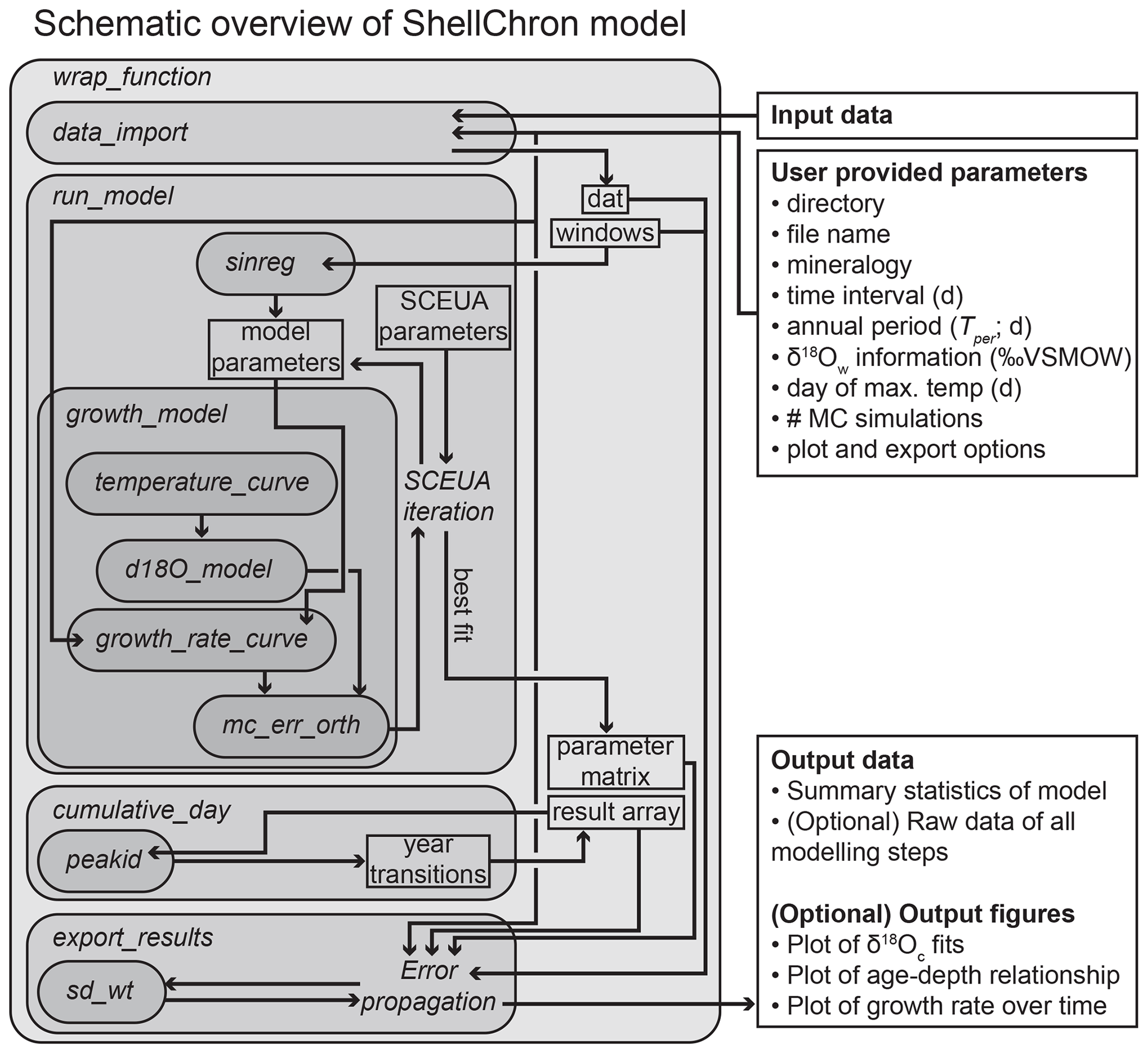
Figure 1 Schematic overview of ShellChron. Names in italics refer to functions (encapsulated in rounded rectangular boxes) and operations within functions. Rectangular boxes represent data. Arrows represent the flow of information between model components. Note that some operations are encapsulated in functions (e.g., Error propagation in export results) and that some functions are only used within other functions (e.g., peakid in cumulative_day). All data structures outside wrap_function represent input and output of the model. Detailed documentation of all functions and operations in ShellChron is provided in SI1 (see also the “Code and data availability” section).

Figure 2 (a) Plots of the growth rate (light green), δ¹⁸O_w (blue), and temperature (red) records (in time domain) from which the test case was produced. Black triangles on the bottom of the temperature plot indicate the ages of the samples taken from the record. (b) The δ¹⁸O_c record for the test case generated after equidistant sampling using the seasonalclumped package (de Winter et al., 2021a) with a sampling interval of 0.5 mm. Error bars on sampling distance (0.1 mm) and δ¹⁸O_c (0.1 ‰) fall within the symbols. Vertical grey dashed lines indicate user-provided year markers, and the blue bar on top of this plot shows an example of the width of a modeling window. See the Supplement for details on producing the test case δ¹⁸O_c record and SI3 for the R script used to generate the data.

3 Model description

ShellChron is organized as a series of functions that describe the step-by-step modeling process. A schematic overview of the model is given in Fig. 1. A short test case is used to illustrate the modeling steps in ShellChron. Figure 2 shows how the virtual test case was created from randomly generated seasonal growth rate, δ¹⁸O_w and temperature curves using the seasonalclumped R package (de Winter et al., 2021a; see Fig. 2 and Supplement SI2). A wrapper function (wrap_function) is included, which carries out all steps of the model procedure in succession to promote ease of use.

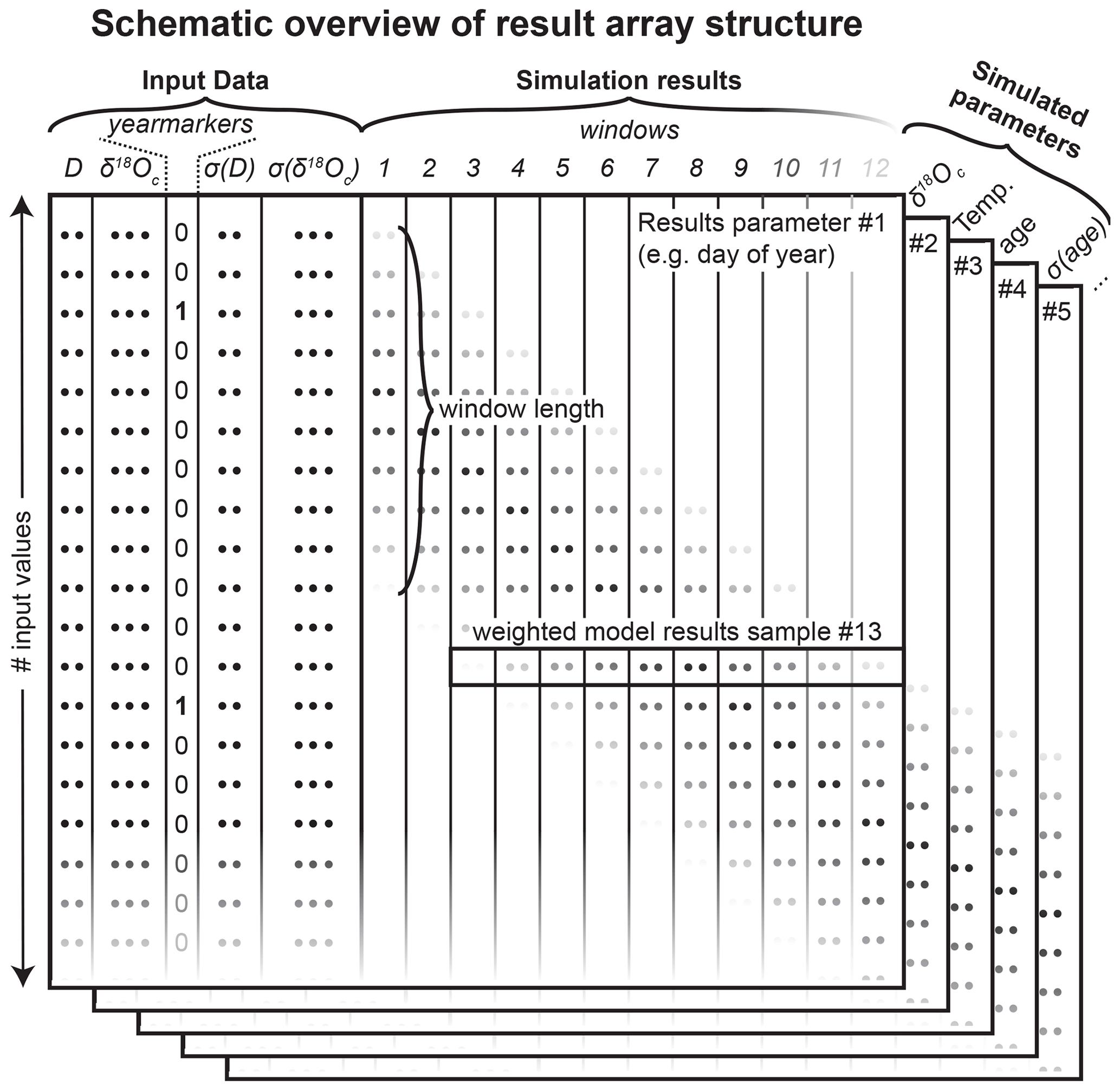
Figure 3 Schematic overview of the structure of the result array in which ShellChron stores the raw results of each model window. Data are stored in three dimensions: the sample number (rows in the figure), the window number (columns in the figure), and the number of modeled parameters (represented by the stacked table “sheets” in the figure). Note that the first five columns of each sheet represent the user-provided input data (see example in SI2) and that the model result data start from column 6. The window length is determined by the user-provided indication of year transitions (column 3). Rows of dots in the figure are placeholders for (input or result) values. Shading of these dots in the window columns indicates differential weighting of modeled values as a function of their location relative to the sliding window. The horizontal box shows how these weighting factors within each sample window (in vertical direction) result in weighting of different estimates of modeled parameters for the same data point (in horizontal direction). The shading of input data and window number towards the bottom and right edge of the figure, respectively, indicates that the number of input values (and thus simulation windows) is only limited to the length of the input table and may therefore continue indefinitely (at the expense of longer computation times; see Fig. 8 in the “Model performance” section).

Data are imported through the data_import function, which takes a comma-separated value (CSV) text file with the input data. Data files need to contain columns containing sampling distance (D, in µm) and δ¹⁸O_c data (in ‰ VPDB), a column marking years in the record (yearmarkers), and two optional columns containing uncertainties in sampling distance (σ(D), 1 standard deviation; µm) and δ¹⁸O_c (σ(δ¹⁸O_c), 1 standard deviation; ‰) (see example in SI2 and Fig. 3). The function uses the year markers (third column) as guidelines for defining the minimum length of the model windows to ensure that all windows contain at least 1 year of growth. By default, consecutive windows are shifted by one data point, yielding a total number of windows equal to the sample size minus the length of the last window. While year markers are required for ShellChron to run (otherwise no windows can be defined), the result of the model does not otherwise depend on user-provided year markers, instead basing the age result purely on simulations of the δ¹⁸O_c data.

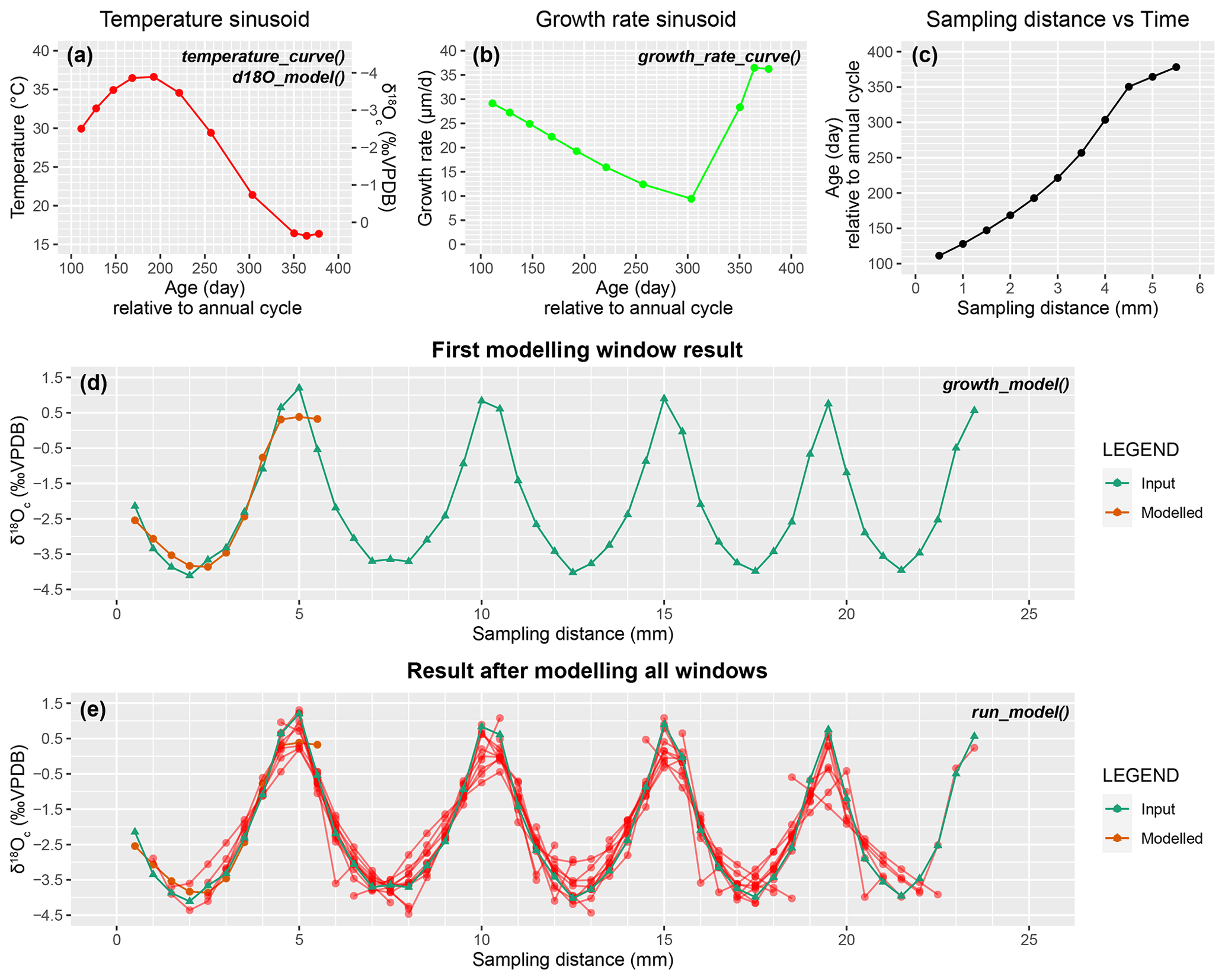
Figure 4 Showing the steps taken to simulate δ¹⁸O_c data in the run_model function on the test case. (a) Temperature sinusoid used to approximate δ¹⁸O_c data in the first modeling window (see panel d), produced using a combination of temperature_curve and d18O_model functions. Symbols indicate the positions of δ¹⁸O_c samples on the temperature curve, with estimated δ¹⁸O_c values shown on the secondary axis (right). (b) Skewed growth rate sinusoid fit to the δ¹⁸O_c data using the growth_rate_curve function. Note the shift towards steeper growth rate increase around the 300th model day (autumn season in this example). See Fig. S2 for a detailed description of the growth rate sinusoid. (c) The modeled age–distance relationship for this window after fitting δ¹⁸O_c data, resulting from aligning the estimated age of samples (x axes in panel a) with the distance in sampling direction (x axis in panel d) using the cumulative growth rate function (b). (d)  δ¹⁸O_c profile of the test case (green) with the δ¹⁸O_c curve of the first modeling window (red), which results from the combination of temperature (a) and growth rate (b) sinusoids, plotted on top (growth_model function). (e) Result after simulating the full δ¹⁸O_c profile of the test case (green) using run_model, with the δ¹⁸O_c curves of individual modeling windows shown in red.

The core of the model consists of simulations of overlapping subsamples (windows) of the sampling distance and δ¹⁸O_c data described by the run_model function (see Figs. 1 and 3). Data and window sizes are passed from data_import to run_model along with user-provided parameters (e.g., δ¹⁸O_w information; see Fig. 1). The run_model function loops through the data windows and calls the growth_model function, which fits a modeled δ¹⁸O_c vs. distance curve through the data using the SCEUA optimization algorithm (see Duan et al., 1992; see example in Fig. 4). The simulated δ¹⁸O_c curve is produced through a combination of a temperature sinusoid (temperature_curve function; see Eq. 4, Figs. 4a and S1) and a skewed growth rate sinusoid (growth_rate_curve; see Eq. 5, Figs. 4b and S2), with temperature data converted to δ¹⁸O_c data through the d18O_model function (Eqs. 1 and 2; Fig. 4a).

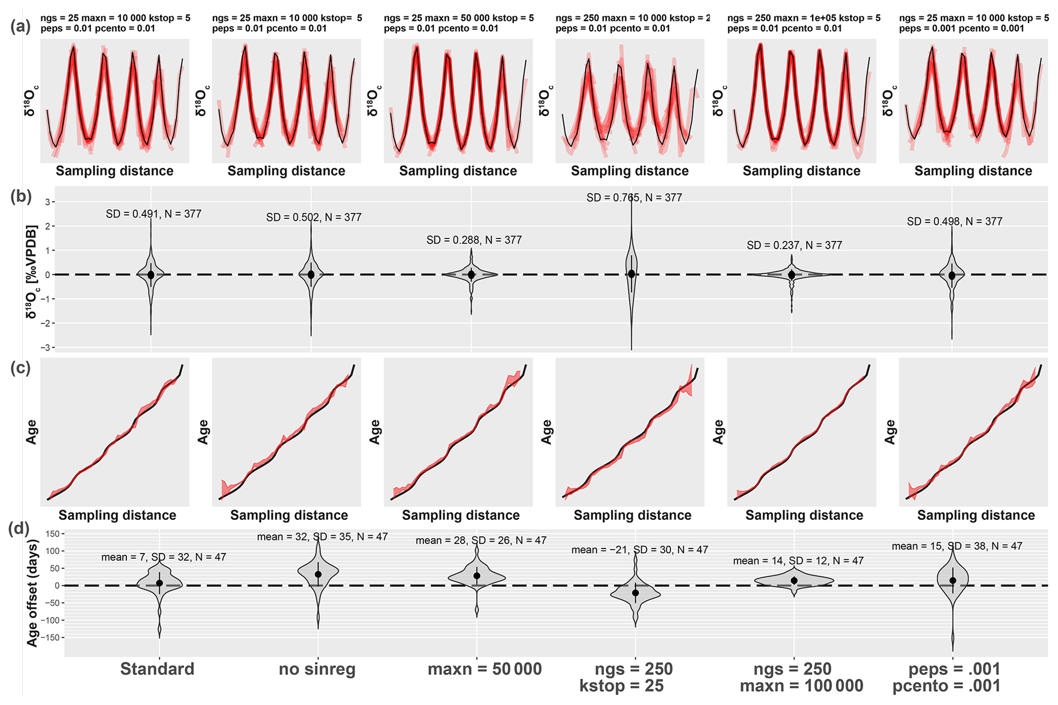
Figure 5 Result of testing ShellChron with various combinations of SCEUA parameters and sinusoidal regression on the test case dataset (see Fig. 2). The leftmost plots illustrate performance of ShellChron under default SCEUA parameters. Plots to the right show various combinations of parameters that deviate from the default (see labels on top and bottom of plot). (a) Fits of the model δ¹⁸O_c curves (red) with the data (black). (b) Violin plots showing the distribution of modeled δ¹⁸O_c offset from the data. (c) Age–distance plots showing modeled (red) and known (black) age–depth relationships for each scenario. (d) Violin plots showing the distribution of age offsets from the known age–depth relationship. SD: standard deviation, N: number of data points, sinres: sinusoidal regression; maxn, ngs, kstop, peps, and pcento are SCEUA parameters (see Duan et al., 1992, and explanation in Sect. 4.1). Data on test results are provided in SI11.

By default, starting values for the parameters describing temperature and growth rate curves are obtained by estimating the annual period (P) through a spectral density estimation and applying a linearized sinusoidal regression through the δ¹⁸O_c data (sinreg function; see Eq. 9). It is possible to skip this sinusoidal modeling step through the sinfit parameter in the run_model function, in which case the starting value for the annual period is set equal to the width of the model window. In addition, growth_model takes a series of parameters describing the method for SCEUA optimization (see Duan et al., 1992; Judd et al., 2018) and the upper and lower bounds for parameters describing temperature and growth rate curves (see SI4). Parameters for the SCEUA algorithm (iniflg, ngs, maxn, kstop, pcento, and peps) in the run_model function may be modified by the user to reach more desirable optimization outcomes. The effect of changing the SCEUA parameters on the model result for the test case is illustrated in Sect. 4.1 (see Fig. 5). If uncertainties in sampling distance and δ¹⁸O_c data are provided, growth_model calls the mc_err_orth function to propagate these errors through the model result (see Eq. 6 and Fig. S3).

$${\mathit{\delta }}^{\mathrm{18}}{\mathrm{O}}_{\mathrm{c}}\left[\mathrm{‰}\text{ VPDB}\right]=I+{\displaystyle \frac{A}{\mathrm{2}}}\sin \left({\displaystyle \frac{\mathrm{2}\mathit{\pi }\cdot \left(D-\mathit{\phi }+\frac{P}{\mathrm{4}}\right)}{P}}\right)$$

linearized as

$${\mathit{\delta }}^{\mathrm{18}}{\mathrm{O}}_{\mathrm{c}}\left[\mathrm{‰}\text{ VPDB}\right]=a+b\sin \left({\displaystyle \frac{\mathrm{2}\mathit{\pi }}{P}}\cdot D\right)+c\cos \left({\displaystyle \frac{\mathrm{2}\mathit{\pi }}{P}}\cdot D\right)$$

with

$$\begin{array}{}\text{(9)}& I=a;A=\sqrt{b^{\mathrm{2}}+c^{\mathrm{2}}}\text{ and }\mathit{\phi }=P\cdot \left(\mathrm{0.25}-{\displaystyle \frac{{\cos }^{-\mathrm{1}}\left(\frac{b}{A}\right)}{\mathrm{2}\mathit{\pi }}}\right)\end{array}$$

The run_model function returns an array listing day of the year (1–365), temperature, δ¹⁸O_c, growth rate, and (optionally) their uncertainty standard deviations as propagated from uncertainties in the input data (“result array”; see Fig. 3 and SI5). Note that the default length of the year (Tper and Gper) is set at 365 d, but these parameters can be modified by the user in run_model. In addition, a matrix containing the optimized parameters of temperature and growth rate curves is provided, yielding information about the evolution of mean values, phases, amplitudes, and skewness of seasonality in temperature and growth rate along the record (“parameter matrix”; see Fig. 1 and SI6). To construct an age model for the entire record, the modeled timing of growth data, expressed as day relative to the 365 d year, is converted into a cumulative time series listing the number of days relative to the start of the first year represented in the record (rather than relative to the start of the year in which the data point is found). This requires year transitions (transitions from day 365 to day 1) to be recognized in all the model results. The cumulative_day function achieves this by aggregating information about places where the beginning and end of the year are recorded in individual window simulations and applying a peak identification algorithm (peakid function) to find places in the record where year transitions occur (see the Supplement). Results of the timing of growth for each sample (in day of the year) are converted to a cumulative timescale using their positions relative to these recognized year transitions (Supplement).

In a final step (described by the export_results function), the results from overlapping individual modeling windows are combined to obtain mean values and 95 % confidence envelopes of the result variables (age, δ¹⁸O_c, δ¹⁸O_c-based temperatures, and growth rates) for each sample in the input data. If uncertainties in the input variables were provided, these are combined with uncertainties in the modeling result calculated from results of the same data point on overlapping data windows by pooling the variance of the uncertainties (Eq. 10). Throughout this merging of data from overlapping windows, results from data points on the edge of windows are given less weight than those from data points near the center of a window (see Eq. 7 and Fig. S4). This weighting procedure corrects for the fact that data points near the edge of a window are more susceptible to small changes in the model parameters and are therefore less reliable than results in the center of the window. Finally, summaries of the simulation results and the model parameters including their confidence intervals are exported as comma-separated value (CSV) files. In addition, export_results supports optional exports of figures displaying the model results and files containing raw data from all individual model windows (equivalent to sheets of the result array; see Fig. 3 and SI5):

$$\begin{array}{}\text{(10)}& {\text{VAR}}_{\mathrm{pooled}}={\displaystyle \frac{\sum _i\left(\left(N_i-\mathrm{1}\right)\cdot {\text{VAR}}_i\cdot w_i\right)}{\sum _i\left(N_i\right)-n}},\end{array}$$

in which w is the weight of the individual reconstructions, N is the sample size, and n is the number of reconstructions (indexed by i) that are combined.

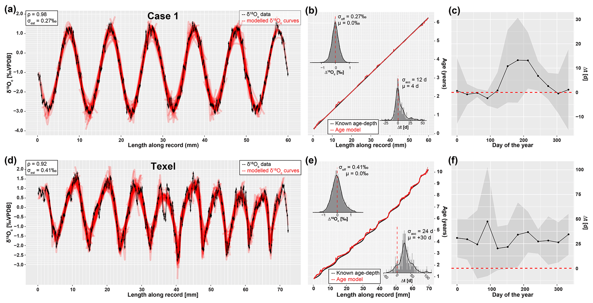
Figure 6 Result of applying ShellChron to two virtual datasets: Case 1 (top, see SI8) and Texel (bottom, see SI9). Leftmost panels (a, d) show the model fit of individual sample windows (red) on the data (black, including horizontal and vertical error bars), with Spearman's correlation coefficients (ρ) in the top left and standard deviations of the δ¹⁸O_c estimate (σ_est). Middle panels (b, e) show the resulting age model (red, including shaded 95 % confidence level) compared with the known age–distance relationship of both records. Histograms in the top left of age–distance plots show the offset between modeled and measured δ¹⁸O_c (as visualized in panels a and d) with standard deviations of the δ¹⁸O_c offset (σ_off) and offset averages (μ). Histograms in the bottom right of age–distance plots show the offset between modeled and known ages (in days) of each data point, including standard deviations of the age accuracy (σ_acc) and mean age offset (μ). Rightmost panels (c, f) highlight age offsets binned in 12 monthly time bins based on their position relative to the annual cycle to illustrate how accuracy varies over the seasons. Grey envelopes indicate 95 % confidence levels for the monthly age offset within these monthly time bins. The horizontal red dashed line indicates no offset (modeled age is equal to the known age of the sample).

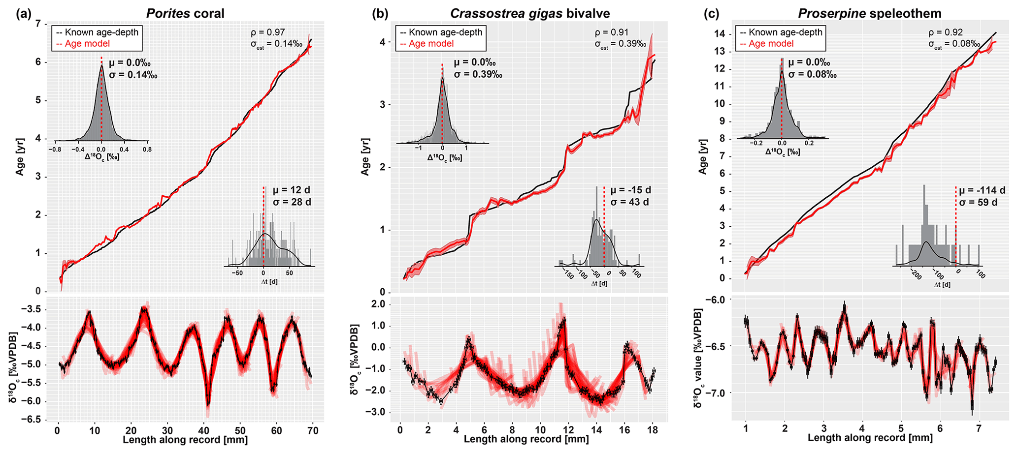
Figure 7 Overview of model results for the three test datasets from real carbonate archives: (a) coral, (b) oyster, and (c) speleothem. Lower panels indicate the fit of individual model windows (in red) with the data (in black), while upper panels show the age model (in red) compared to the “true” age–distance relationship with histograms showing model accuracy (in days, top left) and model fit (δ¹⁸O_c offset in ‰, bottom right). Color scheme follows Fig. 3. Note that the true age–distance relationship is not known for these natural records but is estimated using known growth seasonality (coral), comparison with in situ temperature and salinity measurements (oyster), or simply by interpolating between annual growth lines (speleothem). See the Supplement for details and SI10 for raw data.

4 Model performance

The performance of ShellChron was first tested on three virtual datasets:

1. the short test case used to illustrate the model steps above (see Figs. 2 and 4; SI7),

2. a δ¹⁸O_c record constructed from a simulated temperature sinusoid with added stochastic noise (Case 1; SI8), and

3. a record based on a known high-resolution sea surface temperature and salinity record measured on the coast of Texel island in the tidal basin of the Wadden Sea (northern Netherlands; Texel, see details in SI9 and de Winter et al., 2021a, as well as the Supplement).

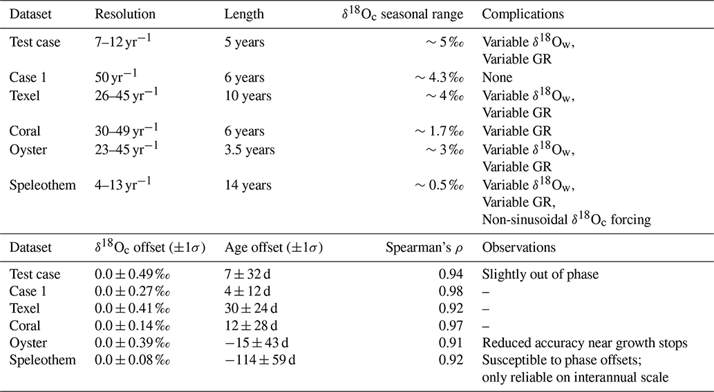
Firstly, the effect of varying parameters in the SCEUA algorithm is tested on the test case (Fig. 5). Then, full model runs on Case 1 and Texel are evaluated in terms of model performance (Fig. 6). In addition to the three test cases, three modern carbonate δ¹⁸O_c records were internally dated using ShellChron (see Fig. 7): a tropical stony coral (Porites lutea; hereafter: coral) from the Pandora Reef (Great barrier Reef, NE Australia; Gagan et al., 1994; see SI10), a Pacific oyster shell (Crassostrea gigas; hereafter: oyster) from List Basin in Denmark (Ullmann et al., 2010; see SI10), and a temperate-zone speleothem from Han-sur-Lesse cave (Belgium; hereafter: speleothem; see Vansteenberge et al., 2020; see SI10). Finally, ShellChron's performance in terms of computation time and accuracy is compared to that of the most comprehensive pre-existing δ¹⁸O_c-based age model (GRATAISS model by Judd et al., 2018) on simulated temperature sinusoids of various length and sampling resolutions to which stochastic noise was added (sensu Case 1; de Winter et al., 2021a; see Fig. 8 and SI11). The latter also demonstrates the scalability of ShellChron and its application to a variety of datasets. Timing comparisons were carried out using a modern laptop (Dell XPS13–7390; Dell Inc., Round Rock, Tx, USA) with an Intel Core i7 processor (8 MB cache, 4.1 GHz clock speed, four cores, Intel Corporation, Santa Clara, CA, USA), 16 GB LPDDR3 RAM and an SSD drive running Windows 10. Note that ShellChron was built and tested successfully on Mac OS, Fedora Linux, and Ubuntu Linux as well.

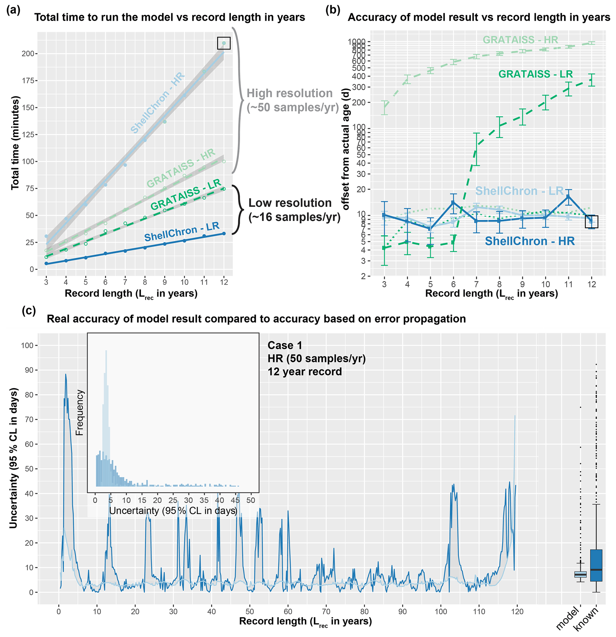
Figure 8 Overview of the result of timing ShellChron and the GRATAISS model on the same datasets (a), comparing the accuracies of both models (b), and comparing the accuracy as calculated by ShellChron with the known offset in the age model (c). In (a) and (b), low-resolution datasets are plotted in dark blue (ShellChron) and dark green (GRATAISS), while high-resolution datasets are plotted in light blue (ShellChron) and light green (GRATAISS). Solid lines represent ShellChron, and dashed lines show the performance of the GRATAISS model. Green dotted lines in (b) show the accuracies of the GRATAISS model on a year-by-year basis (without accumulating error due to linking consecutive years). The black box in (a) and (b) highlights the dataset used in (c). In (c), dark blue lines, bars, and box plot indicate true offset of the model from the actual sample age, while light blue lines, bars, and box plot show the accuracy of the model as calculated from the propagated errors in model and input data. Raw data are provided in SI11.

4.1 Testing model parameters

Testing different combinations of modeling parameters (Fig. 5) shows that, while the results of ShellChron can improve beyond the default SCEUA parameters and sinusoidal regression, care must be taken to evaluate the effect of changing modeling parameters on both the δ¹⁸O_c fit and the age–distance relationship. Comparative testing on the test case (Fig. 5) shows that sinusoidal regression has a negligible influence on the success of ShellChron fitting the δ¹⁸O_c curve (Fig. 5a and b; standard deviation for δ¹⁸O_c is 0.49 ‰ with sinusoidal regression and 0.50 ‰ without). However, ShellChron with sinusoidal regression performs better in terms of age approximation, with a mean age offset of only 7±32 d with sinusoidal regression against 32±35 d without (Fig. 5c and d). Age–distance plots (Fig. 5c) show that the model without sinusoidal fit shows a phase offset with respect to the known age–distance relationship, resulting in overestimation of the age for much of the record. Sinusoidal regression probably results in better initial parameter estimation, which helps to avoid phase offsets like the one shown in Fig. 5. For the remainder of the tests, sinusoidal regression was enabled.

The remainder of the tests show that the main bottleneck towards better δ¹⁸O_c fit optimization is the maximum number of function evaluations allowed within a single modeling cycle (maxn; see Fig. 5). Increasing the other SCEUA parameters, such as the number of complexes in the SCEUA routine (ngs), the number of shuffling loops that should show a significant change before convergence (kstop), and the thresholds for significant change in parameter value (peps) or result value (pcento), does not improve the result if the SCEUA algorithm is not allowed more processing time (maxn). In fact, Fig. 5 shows that increasing these SCEUA parameters can actually result in a deterioration of the δ¹⁸O_c fit and higher uncertainty in the age result (Fig. 5b and d). A fivefold increase in maxn (maxn = 50 000) almost halves the standard deviation of δ¹⁸O_c residuals (from 0.49 ‰ to 0.29 ‰; Fig. 5b) and decreases the standard deviation of the age model offset from 32 to 26 d (Fig. 5d). A combination of a 10-fold increase in function evaluations with an equal multiplication of the number of complexes in the SCEUA routine (ngs; see details in Duan et al., 1992) results in a further reduction of standard deviations of δ¹⁸O_c (0.23 ‰) and age results (12 d). These tests show that returns in terms of model precision quickly diminish with increasing processing time. Since the total modeling time linearly scales with the number of function evaluations, this trade-off towards a lower standard deviation of the modeling result is costly. These function evaluations are repeated in each modeling window, so the cost in terms of extra processing time can increase quickly, especially for larger δ¹⁸O_c datasets. In addition, in this situation the mean model offset (accuracy of the model; 7, 28 and 14 d for maxn of 1.0×10⁴, 5.0×10⁴ and 1.0×10⁵, respectively; Fig. 5d) does not significantly improve with an increasing number of function evaluations. Based on these results, the default maxn parameter in ShellChron was set to 10⁴ to compromise between keeping modeling times short while retaining high model accuracy. However, specific datasets may benefit from an increase in modeling time, so case-by-case assessment of the optimal SCEUA parameters is recommended. A detailed evaluation of the total modeling time in a typical δ¹⁸O_c dataset is discussed in Sect. 4.4.

Table 2 Overview of datasets and model results.

4.2 Artificial carbonate records

Results of running ShellChron on the test case (Fig. 4), Case 1, and Texel datasets (Fig. 6) show that modeled δ¹⁸O_c records in individual windows closely match the data. On the level of individual windows, interannual growth rate variability is more difficult to model than the temperature sinusoid, especially when sampling resolution is limited and at the beginning and end of the record (Fig. 4b). However, after overlapping multiple windows, the accuracy of ShellChron improves significantly (Fig. 4e). Note that in Fig. 4a–c, the length of the first model window (difference in age between first and 11th data point) is less than 365 d because the 12th data point, which occurs exactly 1 year after the first point, is not part of the window. A summary of ShellChron performance statistics is given in Table 2. In all virtual datasets, δ¹⁸O_c estimates are equally distributed above and below the δ¹⁸O_c data ($\stackrel{\mathrm{‾}}{{\mathrm{\Delta }}^{\mathrm{18}}{\mathrm{O}}_{\mathrm{c}}}=\mathrm{0.0}\mathrm{‰}$; Spearman's ρ of 0.94, 0.98, and 0.92 for the test case, Case 1, and Texel datasets, respectively). Age offsets vary slightly over the seasons, but the difference between monthly time bins is not statistically significant on a 95 % confidence level (Fig. 6c and f; see also SI12). The fact that seasonal bias in age offset is absent in the Texel dataset, which is skewed towards growth in the winter season and includes relatively strong seasonal variability in δ¹⁸O_w, shows that ShellChron is not sensitive to such subtle (though common) variability in growth rate or δ¹⁸O_w. In general, ShellChron's mean age assignment is accurate on a monthly scale (age offsets of 4±12 d and $+\mathrm{30}\pm \mathrm{24}$ d for Case 1 and Texel datasets, respectively). However, age results in individual months do sometimes show significant offsets from the known value (e.g., Fig. 6c and f). This is most notable in Case 1, for which the accuracy of the age model decreases near the extreme values of the δ¹⁸O_c curve (Fig. 6b and c). This occurs because in these places the model is most sensitive to stochastic noise (simulated uncertainty) in the δ¹⁸O_c value. A small random change in the δ¹⁸O_c value at the minima or maxima of the δ¹⁸O_c curve thus results in a large change in the model fit of the δ¹⁸O_c curve, resulting in a seasonally nonuniform decrease in the accuracy of the model, as is evident from the skewed Δ¹⁸O_c distribution in Fig. 6b and c. The sampling resolution in the Texel data decreases near the end of the record (see SI9), but this does not result in reduced age model accuracy. If anything, the age of Texel samples is better approximated near the end of the record, and age offsets are larger in the central part of the record (∼30–50 mm; Fig. 6e). The lower accuracy in the third to fifth year of the Texel record is likely a result of the sub-annual variability in the record that is superimposed on the seasonal cycle. The lower sampling resolution later in the record mutes this variability and illustrates that higher sampling resolutions do not necessarily result in better age models. The constant offset of the modeled age of the Texel sample from the known age is a result of the way the model result was aligned to start at zero for comparison with the known age (Fig. 6f). This was done by adding the offset from zero of the modeled age of the first data point in the record to the entire record, thereby defining an arbitrary reference point which is sensitive to the uncertainty in the age of the first sample (see also oyster and speleothem results in Fig. 7b and c). Note that this alignment issue does not play a role in fossil data, for which model results can be aligned to growth marks in the carbonate (e.g., shell growth breaks or laminae), and that it does not affect the seasonal alignment of the proxy binned into monthly sample bins.

4.3 Natural carbonate records

Results of modeling natural carbonate records (Fig. 7; Table 2; see also SI10) illustrate the effectiveness of ShellChron for various types of records. Performance clearly depends on the resolution of the record and the regularity of seasonal variability contained within. As in the virtual datasets, modeled δ¹⁸O_c successfully mimics δ¹⁸O_c data in all records ($\stackrel{\mathrm{‾}}{{\mathrm{\Delta }}^{\mathrm{18}}{\mathrm{O}}_{\mathrm{c}}}=\mathrm{0.0}$; Spearman's ρ of 0.97, 0.91, and 0.92 for coral, oyster, and speleothem, respectively). No consistent seasonal bias is observed in Δ¹⁸O_c and model accuracy (p>0.05; see Table 2 and SI12), despite significant (seasonal and interannual) variability contained in the records (especially in oyster and speleothem records). When comparing the accuracy of these records, it must be noted that the “known” age of the samples in these natural carbonates is not known. Model results are instead compared with age models constructed using conventional techniques such as matching δ¹⁸O_c profiles with local temperature and/or δ¹⁸O_w variability (oyster and coral records) or even merely by linear interpolation between annual markers in the record (speleothem record; see the Supplement). Despite this caveat, testing results clearly show that the least complicated record (coral; Fig. 7A), characterized by minimal variability in δ¹⁸O_w and growth rate as well as a high sampling density, has the best overall model result (Δ¹⁸O${}_{\mathrm{c}}=\mathrm{0.0}\pm \mathrm{0.14}$ compared to a ∼1.7 ‰ seasonal range; ρ=0.97; $\mathrm{\Delta }t=\mathrm{12}\pm \mathrm{28}$ d; see Table 2). The oyster record (Fig. 7b), which has strong seasonal variability in growth rate and δ¹⁸O_sw, also yields a reliable age model (Δ¹⁸O${}_{\mathrm{c}}=\mathrm{0.0}\pm \mathrm{0.39}$ compared to a ∼3 ‰ seasonal range; ρ=0.91; $\mathrm{\Delta }t=-\mathrm{15}\pm \mathrm{43}$ d; see Table 2). On closer inspection, the age within the oyster record is clearly more difficult to model than within the coral, due in part to the higher variability of δ¹⁸O_c values superimposed on the seasonal cycle, the sharp growth cessations in the winters (high δ¹⁸O_c values), and the variability in sampling resolution within the record. The latter causes the first growth year of the oyster record to be less accurately modeled (Fig. 7b), while the variability in δ¹⁸O_c causes the edges of some modeling windows to predict steep increases or decreases in δ¹⁸O_c (vertical “offshoots” in modeled δ¹⁸O_c; Fig. 7b). Note that the low weighting of the edges of modeling windows combined with the high overall sampling resolution in the oyster record minimizes the effect of these offshoots on the accuracy of the model. The speleothem record (Fig. 7c), plagued by lower sampling resolution, large interannual δ¹⁸O_c variability, restricted δ¹⁸O_c seasonality, and a lack of clearly seasonal δ¹⁸O_c forcing, yields the least reliable model result (Δ¹⁸O${}_{\mathrm{c}}=\mathrm{0.0}\pm \mathrm{0.08}$ ‰ compared to a ∼0.5 ‰ seasonal range; ρ=0.92; $\mathrm{\Delta }t=-\mathrm{114}\pm \mathrm{59}$ d; see Table 2). Note that the accuracy figure provided for the speleothem record is based on comparison with an age model relying on linear interpolation between annual growth lines. This assumption of the age–distance relationship is almost certainly erroneous, since drip water supply to (and therefore growth in) speleothems has been shown to vary seasonally (e.g., Baldini et al., 2008), including at the very site the speleothem data derive from (Han-sur-Lesse cave, Belgium; Van Rampelbergh et al., 2014; Vansteenberge et al., 2020). However, since no reliable information is available on sub-annual variability in growth rates in this record, ShellChron results cannot be validated at the sub-annual scale in this case. The high age offset (−114 d) in the speleothem model result is a consequence of the assumption in ShellChron that the highest temperature (lowest δ¹⁸O_c value) recorded in each growth year happens halfway through the year (day 183) and the alignment of the modeled age with the known age for this record (see discussion of Texel results in Sect. 4.2). While the assumption about the phase of the temperature sinusoid is approximately valid for temperature-controlled δ¹⁸O_c records (see Figs. 6 and 7), it is problematic for speleothems, in which δ¹⁸O_c is often dominated by the δ¹⁸O_w of drip water, which may not be lowest during the summer season (see Van Rampelbergh et al., 2014). The timing of the δ¹⁸O_c minimum can be set in the run_model function using the t_maxtemp parameter. Note that changing t_maxtemp does not affect relative dating within the δ¹⁸O_c record but, if set correctly, results in a phase shift of the age model result into better alignment with the seasonal cycle.

4.4 Modeling time

The performance of both ShellChron and GRATAISS in terms of computation time linearly increases with the length of the record (in years; see Figs. 8, S5 and SI11). Computation time of ShellChron for the high-resolution test dataset (50 samples yr⁻¹) increases very steeply with the length of the record in years (∼20 min per additional year), while the low-resolution dataset (16 samples yr⁻¹) shows a slower increase (∼3 min per additional year; Fig. 5a). This contrasts with GRATAISS, which requires only slightly more time for high-resolution data than low-resolution datasets (∼7 and ∼10 min per additional year, respectively). The difference is explained by the sliding window approach applied in ShellChron, which requires more SCEUA optimization runs per year in high-resolution datasets than in low resolution datasets. When plotted against the number of calculation windows or samples in the dataset, running ShellChron on low-resolution and high-resolution datasets require a similar increase in computation time (∼0.4 min, or 24 s, per additional sample or window; Fig. S5) under default SCEUA conditions. ShellChron outcompetes GRATAISS in terms of computation time in datasets with fewer than ∼20 samples yr⁻¹, even though more SCEUA optimizations are required.

A key computational improvement in ShellChron is the application of a sinusoidal regression before each SCEUA optimization to estimate the initial values of the modeled parameters (sinreg function; see Eq. 9 and Fig. 1 in Model description). Since carbonate archives are rarely sampled for stable isotope measurements above 20 samples yr⁻¹ (e.g., Goodwin et al., 2003; Schöne et al., 2005; Lough, 2010, and references therein), the disadvantage of a steep computational increase for very high-resolution archives is, in practice, a favorable trade-off for the added control on model and measurement uncertainty as well as smoother inter-year transitions ShellChron offers in comparison to previous models. The similarity of ShellChron's accuracy in the low- and high-resolution datasets demonstrates its robustness across datasets with various sampling resolutions (see also Table 2 and Fig. 7).

Longer computation times in GRATAISS result in slightly better accuracy for the modeled age compared to ShellChron on the scale of individual data points in low-resolution datasets (see Fig. 8b). However, this advantage is rapidly lost when records containing multiple years are considered (Fig. 8b). The advantage of the ShellChron model is its application of overlapping model windows, which smooth out the transitions between modeled years and eliminate accumulations of model inaccuracies when records grow longer. In addition, contrary to previous models, ShellChron does not rely on user-defined year boundaries, which may introduce mismatches between subsequent years to be propagated through the age model, even in ideal datasets such as Case 1 (Fig. 8b; see also the Supplement). By comparison, the overall accuracy of ShellChron is much more stable within and between datasets of different length, while rarely introducing offsets of more than a month. It must be noted here that the cumulative multiyear age uncertainty in the GRATAISS model (Fig. 8b) was calculated by combining the results of consecutive growth years in the record, which GRATAISS models separately, while avoiding age inversions and retaining the seasonal phase of the model results. This procedure causes gaps in time to be introduced in the cumulative age modeled by GRATAISS whenever the results of two consecutive, individually modeled growth years do not align, explaining the sharp increases in age uncertainty of the GRATAISS model result (Fig. 8b). These cumulative uncertainties are therefore not theoretically part of the model result (see year-by-year uncertainty in Fig. 8b) but are a necessary consequence of the way GRATAISS approximates growth years separately. If only within-year inaccuracies are compared, GRATAISS results are roughly equally as accurate as ShellChron results (see dotted lines in Fig. 8b).

While ShellChron considers the uncertainty in input parameters, this uncertainty is not considered in most previous models (the MoGroFun model of Goodwin et al., 2003, being the exception). The added uncertainty caused by input error is higher in less regular (sinusoidal) δ¹⁸O_c records and in records with lower sampling resolution, causing the uncertainties in GRATAISS reported here for the ideal high-resolution Case 1 dataset to be overly optimistic. If ShellChron's model accuracy is insufficient, its modular character allows the user to run the SCEUA algorithm to within more precise optimization criteria by changing the model parameters (see Sect. 4.1). However, this adaptation comes at a cost of longer computation times.

The estimated uncertainty envelope (95 % confidence interval) for the modeled age calculated by the error propagation algorithm in ShellChron (4.7±6.5 d) on average slightly underestimates the actual offset between modeled age and known age in the Case 1 record (9.3±13.1 d; Fig. 8c). The foremost difference between modeled and known uncertainty in the result is that the modeled uncertainty yields a more smoothed record of uncertainty compared to the record of actual offset of the model (Fig. 8c). ShellChron's uncertainty calculations are partly based on comparing overlapping model windows, thereby smoothing out short-term variations in model offset. The uncertainty of the model result (both known and modeled) shows regular variability with a period of half a year (Fig. 8c). Comparing this variability with the phase of the record (6 years of which are plotted in Fig. 6a) reveals that the uncertainty of the model is negatively correlated with the slope of the δ¹⁸O_c record. This is expected because in parts of the record with extreme values in the δ¹⁸O_c curve, the local age model result is more sensitive to small changes in the sampling distance, caused either by uncertainty in the model fit or propagated uncertainty in the sampling distance defined by the user (see discussion in Sect. 4.2). The slight seasonal variability in model accuracy in Case 1 is also shown in Fig. 6c and comprises a difference in uncertainty of up to 10 d depending on the time of year in which the data point is found.

5 Applications and discussion

Its new features compared to previous age model routines make ShellChron a versatile package for creating age models in a range of high-resolution paleoclimate records. The discussion above demonstrates that ShellChron can reconstruct the age of individual δ¹⁸O_c samples with monthly precision. This level of precision is sufficient for accurate reconstructions of seasonality, defined as the difference between warmest and coldest month (following USGS definitions; O'Donnell and Ignizio, 2012). While an improvement on this uncertainty could be of potential interest for ultrahigh-resolution paleoclimate studies (e.g., sub-daily variability; see Sano et al., 2012; Yan et al., 2020; de Winter et al., 2020a), the increase in computation time and the sampling resolution such detailed age models demand render age modeling from δ¹⁸O_c records inefficient for this purpose (see Sect. 4.1 and 4.4). The sampling resolution for high-resolution carbonate δ¹⁸O_c records in the literature does not typically exceed 100 µm due to limitations in sampling acquisition (e.g., micromilling), which even in fast-growing archives limits the resolution of these records to several days at best (see Gagan et al., 1994; Van Rampelbergh et al., 2014; de Winter et al., 2020c). While in some archives, high-resolution (<100 µm) trace element records could be used to capture variability beyond this limit, the monthly age resolution of ShellChron is sufficient for most typical high-resolution paleoclimate studies.

The ability to produce uninterrupted age models from multiyear records while considering both variability in δ¹⁸O_w and uncertainties in input parameters represents major advantages of ShellChron over previous age modeling solutions. As a result, ShellChron can be applied to a wide range of carbonate archives (see Fig. 7 and Table 2). However, testing ShellChron on different records highlights the limitations of the model inherited through its underlying assumptions. The most accurate model results are obtained for records with minimal growth rate and δ¹⁸O_w variability as well as a nearly sinusoidal δ¹⁸O_c record, such as tropical coral records (Fig. 7a; Gagan et al., 1994). In records wherein large seasonal variability in growth rate and δ¹⁸O_w does occur, such as in intertidal oyster shells, ShellChron's accuracy slightly decreases, especially near growth hiatuses in the record (see Fig. 7b; Ullmann et al., 2010). A worst-case scenario is represented by the speleothem record, which not only suffers from much slower and more unpredictable growth rates and contains a comparatively small annual range in δ¹⁸O_c, but it also responds to δ¹⁸O_w variability in drip water in the cave rather than temperature seasonality, which is one of the assumptions underlying the current version of ShellChron (Fig. 7c; Vansteenberghe et al., 2019). Despite these problems, ShellChron yields an age model that is remarkably accurate on an annual timescale, which is as good as, or better than, the best age model that can be obtained by applying layer counting to the most clearly laminated parts of the speleothem (e.g., Verheyden et al., 2006). It must be noted that, while the close fit between modeled δ¹⁸O_c and speleothem δ¹⁸O_c data (ρ=0.92; σ=0.08 ‰) is encouraging, a major reason for the model's success is the fact that the Proserpine speleothem used in this example is known to receive significantly seasonal (though not sinusoidal) drip water volumes and concentrations (Van Rampelbergh et al., 2014). Variability in drip water properties and cave temperatures is known to differ strongly between cave systems (Fairchild et al., 2006; Lachniet, 2009). For ShellChron (or any other δ¹⁸O_c-based age model) to work reliably in speleothem records, consistent seasonal variability in either temperature or δ¹⁸O_w should be demonstrated to significantly influence the δ¹⁸O_c variability in the record. In practice, these constraints make ShellChron applicable in speleothems for which the cave environment varies in response to the seasonal cycle, such as localities overlain by thin epikarst, well-ventilated caves, or speleothems situated close to the cave entrance (Verheyden et al., 2006; Feng et al., 2014; Baker et al., 2021).

ShellChron's ability to model multiyear records with smooth transitions between the years does not compromise the accuracy of its age determination on the seasonal scale (e.g., Figs. 6 and 7). Many paleoclimatology studies investigating the seasonal cycle rely on stacking of seasonal variability relative to the annual cycle, thereby combining seasonal information from multiple years to obtain a precise reconstruction of seasonal variability in the past (e.g., de Winter et al., 2018; Judd et al., 2019; Tierney et al., 2020). While this can be achieved using age models of individual years (e.g., Judd et al., 2018), seasonally resolved archives dated using ShellChron can also be stacked along a common seasonal axis while retaining information about the multi-annual record, allowing, for example, comparison between consecutive years dated using the same age model including uncertainty in the age determination.

The difficulty of applying age model routines to speleothem records highlights one of the main advantages of ShellChron over pre-existing age model routines, namely its modular character. Since δ¹⁸O_c records from some carbonate archives, such as speleothems, cannot be described by the standard combination of temperature and growth rate sinusoids on which ShellChron is based (in its current version), the possibility to adapt the “building block” functions used to approximate these δ¹⁸O_c records (d18O_model, temperature_curve, and growth_rate_curve; see Fig. 1) while leaving the core structure of ShellChron intact greatly augments the versatility of the model. The freedom to adapt the building blocks used to approximate the δ¹⁸O_c record theoretically enables ShellChron to model sub-annual age–distance relationships in any record if the seasonal variability in the variables used to model the input data are predictable and can be represented by a function. For example, since speleothem δ¹⁸O_c records often depend on variability in the δ¹⁸O_w value of the drip water, a function describing this variability through the year can replace the temperature_curve function to create more accurate sub-annual age models for speleothems (e.g., Mattey et al., 2008; Lachniet, 2009; Van Rampelbergh et al., 2014). Similarly, the growth_rate_curve function can be modified in the case that the default skewed sinusoid does not accurately describe the extension rate of the record under study, and the d18O_model function can be adapted to feature the most fitting δ¹⁸O_c–temperature or δ¹⁸O_c–δ¹⁸O_w relationship. Note that the flexibility of this approach is limited by the expression of the annual cycle in the δ¹⁸O_c record. The δ¹⁸O_c-based dating approach in ShellChron will therefore have more trouble dating records in which the annual δ¹⁸O_c variability is severely dampened, such as speleothems in deeper cave systems (e.g., Vansteenberge et al., 2016), or in which annual δ¹⁸O_c variability is not sinusoidal, such as tropical records with bimodal temperature or precipitation seasonality (Knoben et al., 2019).

Flexibility in the definition of building block functions used to approximate the input data paves the way for future application beyond carbonate δ¹⁸O_c records. The seasonal variability in δ¹⁸O in some ice cores can be approximated by a stable and unbiased temperature relationship (van Ommen and Morgan, 1997). ShellChron can therefore be modified to date sub-annual samples in these ice core records and reconstruct seasonal variability in the high latitudes through the Quaternary. Similarly, interannual δ¹⁸O variability in tree ring records is demonstrated to record variability in precipitation through the year, and this variability can be modeled to improve sub-annual age models in these records (Xu et al., 2016). More generally, the field of dendrochemistry has recently developed additional chemical proxies for seasonality (e.g., trace element concentrations), which can be measured in smaller sample volumes (and thus greater resolution) to obtain ultrahigh-resolution records on which (sub-annual) dating can be based (e.g., Poussart et al., 2006; Superville et al., 2017). A similar development has taken place in the study of carbonate bio-archives such as corals and mollusks, some of which show strong, predictable seasonal variability in trace elements (e.g., $\mathrm{Mg}/\mathrm{Ca}$ and $\mathrm{Sr}/\mathrm{Ca}$ ratios) which can be used to accurately date these records (de Villiers et al., 1995; Sosdian et al., 2006; Durham et al., 2017; de Winter et al., 2021b). Minor changes in the building block functions using empirical transfer functions for these trace element records will enable ShellChron to capitalize on these relationships and reconstruct sub-annual growth rates with improved precision due to the higher precision with which these proxies can be measured compared to δ¹⁸O_c records. Finally, the application of ShellChron for age model construction is not necessarily limited to the seasonal cycle, as other major cycles in climate (e.g., tidal, diurnal, or Milankovitch cycles) leave similar marks on climate records and can thus be used as a basis for age modeling (e.g., Sano et al., 2012; Huyghe et al., 2019; de Winter et al., 2020a; Sinnesael et al., 2019). It must be noted that, since ShellChron was developed for modeling based on annual periodicity, applying it to other timescales would require more thorough adaptation of the model code than merely adapting the building block functions to support additional proxy systems.

While age reconstructions are the main aim of ShellChron, the model also yields information about the temperature and growth rate parameters used in each simulation window to approximate the local δ¹⁸O_c curve (see parameter matrix in Fig. 1 and SI6). These parameters hold key information about the response of the archive to seasonal changes in the environment, such as the season of growth, relationships between growth rate and temperature, and the temperature range that is recorded. Combining these parameters with records of influential environmental variables such as seawater chlorophyll concentration or local precipitation patterns yields information about the response of the climate archive to environmental variables, in addition to the climate or environmental change it records. Study examples include the relationship between the growth rate of marine calcifies and phytoplankton abundance or the correlation between precipitation patterns and chemical variability in speleothems. While such discussion is beyond the scope of this work, examples of parameter distributions are provided in SI5, and the application of modeled growth rate parameters in bivalve sclerochronology is discussed in more detail in Judd et al. (2018). Note that the sliding window approach of ShellChron produces records of changing temperature and growth rate parameters at the scale of individual samples (albeit smoothed by the sliding window approach) rather than annually, as in Judd et al. (2018).

6 Conclusions

ShellChron offers a novel, open-source solution to the problem of dating carbonate archives for high-resolution paleoclimate reconstruction on a sub-annual scale. Based on critical evaluation of previous age models, building on their strengths while attempting to minimize their weaknesses, ShellChron provides continuous age models based on δ¹⁸O_c profiles in these archives with monthly accuracy, considering the uncertainties associated with both the model itself and the input data. The monthly accuracy of the model, as tested on a range of virtual and natural datasets, enables its application for age determination in studies of seasonal climate and environmental variability. Higher accuracies can be reached at the cost of longer computation times by adapting the model parameters, but age determinations far beyond the monthly scale are unlikely to be feasible considering the limitations on sampling resolution and measurement uncertainties in δ¹⁸O_c records. ShellChron's computation times for datasets with sampling resolutions typical for the paleoclimatology field (up to 20 samples yr⁻¹) remain practical and comparable to previous model solutions, despite adding several features that improve the versatility and interpretation of model results. Its modular design allows ShellChron to be adapted to different situations with comparative ease. It thereby functions as a platform for age–distance modeling on a wide range of climate and environmental archives and is not limited in its application to the δ¹⁸O_c proxy, the carbonate substrate, or even to the annual cycle, as long as the relationship between the proxy and the extension rate of the archive on a given timescale can be parameterized. Future improvements will capitalize on this variability, expanding ShellChron beyond its current dependency on the δ¹⁸O_c–temperature relationship in carbonates. Members of the high-resolution paleoclimate community are invited to contribute to this effort by adapting the model for their purpose.