Azimuthal averaging–reconstruction filtering techniques for finite-difference general circulation models in spherical geometry

When solving hydrodynamic equations in spherical or cylindrical geometry using explicit finite-difference schemes, a major difficulty is that the time step is greatly restricted by the clustering of azimuthal cells near the pole due to the Courant–Friedrichs–Lewy condition. This paper adapts the azimuthal averaging–reconstruction (ring average) technique to finite-difference schemes in order to mitigate the time step constraint in spherical and cylindrical coordinates. The finite-difference ring average technique averages physical quantities based on an effective grid and then reconstructs the solution back to the original grid in a piecewise, monotonic way. The algorithm is implemented in a community upper-atmospheric model, the Thermosphere–Ionosphere Electrodynamics General Circulation Model (TIEGCM), with a horizontal resolution up to $\mathrm{0.625}{}^{\circ }\times \mathrm{0.625}{}^{\circ }$ in geographic longitude–latitude coordinates, which enables the capability of resolving critical mesoscale structures within the TIEGCM. Numerical experiments have shown that the ring average technique introduces minimal artifacts in the polar region of general circulation model (GCM) solutions, which is a significant improvement compared to commonly used low-pass filtering techniques such as the fast Fourier transform method. Since the finite-difference adaption of the ring average technique is a post-solver type of algorithm, which requires no changes to the original computational grid and numerical algorithms, it has also been implemented in much more complicated models with extended physical–chemical modules such as the Coupled Magnetosphere–Ionosphere–Thermosphere (CMIT) model and the Whole Atmosphere Community Climate Model with thermosphere and ionosphere eXtension (WACCM-X). The implementation of ring average techniques in both models enables CMIT and WACCM-X to perform global simulations with a much higher resolution than that used in the community versions. The new technique is not only a significant improvement in space weather modeling capability, but it can also be adapted to more general finite-difference solvers for hyperbolic equations in spherical and polar geometries.

Highlights.

• The ring average technique is adapted to solve the issue of clustered grid cells in polar and spherical coordinates with a finite-difference method.

• The ring average technique is applied to develop a $\mathrm{0.625}{}^{\circ }\times \mathrm{0.625}{}^{\circ }$ high-resolution TIEGCM and more complicated geoscientific models with polar and spherical coordinates as well as finite-difference numerical schemes.

• The high-resolution TIEGCM shows good capability in resolving mesoscale structures in the ionosphere–thermosphere (I–T) system.

1 Introduction

Mesoscale structures with a typical horizontal size of 100–500 km have gained more and more attention in research on the dynamics of the upper-atmospheric system. A number of studies have been carried out to investigate these structures, including the formation and evolution of polar cap patches and tongues of ionization (Basu et al., 1995; Foster et al., 2005; Zhang et al., 2013), dynamics of ionospheric irregularities (Makela and Otsuka, 2012; Sun et al., 2015), variations of the polar thermospheric density anomaly (Crowley et al., 2010; Lühr et al., 2004), and the space weather effects of mesoscale electric field variability (Codrescu et al., 1995; Matsuo and Richmond, 2008; Zhu et al., 2018; Lotko and Zhang, 2018). These dynamic mesoscale structures have shown critical importance in understanding the physics of the solar–terrestrial system and in space weather predictions, which challenges the resolution and accuracy of numerical models of the upper-atmospheric system in resolving these important mesoscale signatures.

Spherical or cylindrical coordinates are commonly used in solving geophysical problems, including the modeling of the upper-atmospheric systems. As a workhorse for space weather research, a number of general circulation models (GCMs) for the coupled ionosphere–thermosphere (I–T) system have been developed based on spherical coordinates using finite-difference schemes (e.g., Richmond et al., 1992; Fuller-Rowell et al., 1996; Ridley et al., 2006; Ren et al., 2009). However, restricted by the longitudinal grid resolution, current horizontal resolutions used in I–T GCMs are still insufficient for fully resolving mesoscale atmospheric structures, which are either marginal or sub-grid. The latest released version of the community code, the Thermosphere–Ionosphere Electrodynamic General Circulation Model (TIEGCM), has a longitude–latitude resolution of $\mathrm{2.5}{}^{\circ }\times \mathrm{2.5}{}^{\circ }$. The Coupled Thermosphere–Ionosphere–Plasmasphere (CTIP) model has a latitude resolution of 2^∘ and a longitude resolution of 18^∘, and the most recent version of the Global Ionosphere Thermosphere Model (GITM) has a flexible grid with a latitudinal resolution up to 0.3125^∘, but the typical longitudinal resolution remains 2.5^∘ due to severe time step restrictions for global-scale calculations.

The major difficulty in increasing longitudinal resolution in spherical-geometry-based GCMs is that the explicit time stepping is constrained by the clustering azimuthal cells near the pole due to the Courant–Friedrichs–Lewy (CFL) condition (Courant et al., 1928). A number of attempts have been proposed to address this coordinate singularity issue (e.g., Purser, 1988; Bouaoudia and Marcus, 1991; Williamson et al., 1992; Takacs et al., 1999; Fukagata and Kasagi, 2002; Prusa, 2018). To use a time step that is larger than the global minimum requirement from CFL conditions, one common method used in a spherical GCM is to employ a low-pass Fourier filter at polar latitudes, which removes nonphysical, high-frequency zonal waves generated due to numerical instability caused by the local violation of CFL conditions (e.g., Skamarock et al., 2008). Although the Fourier filter can maintain computational stability and permit a much larger temporal step, the applicability of the fast Fourier transform (FFT) filter method is problem-dependent, which also creates barriers in moving models forward to finer spatial resolutions. Moreover, the linear filtering of zonal components generated through a nonphysical time step may decrease the accuracy of the model calculations near the polar region, which affects physical conservations of, e.g., mass, momentum, and energy that are essential for the long-term behavior of the GCM (Williamson and Browning, 1973).

Recently, Zhang et al. (2019) developed a new technique called the ring average method for hyperbolic equations to mitigate the CFL restrictions in spherical or polar geometry on the basis of the method originally proposed in the Lyon–Fedder–Mobarry (LFM) magnetohydrodynamics (MHD) simulations (Lyon et al., 2004). The method is a “post-solver” type of algorithm applied after solving all the physical quantities in the original spherical coordinates; thus, no modification to the numerical solver or the computational grid is required when applying the ring average. Test simulation results have shown the effectiveness of the ring average algorithm in increasing the time step by a factor of 100 while maintaining the fidelity of the solutions. The original ring average technique was developed for solving hyperbolic equations in spherical or polar geometry based on finite-volume schemes, which redistributes the solution azimuthally through a conservative averaging–reconstruction algorithm. The finite-volume version of the ring average technique not only releases the time step constraint in spherical geometry, but also keeps the conservative nature of finite-volume schemes to machine precision. In this paper, we adapt the ring average technique to finite-difference schemes for solving hyperbolic equations. Defined on an effective reduced polar grid, the finite-difference adaption of the ring average technique also conducts a post-solver step of averaging–reconstruction in each azimuthal ring to maintain the numerical stability and relax the severe computational time step constraint. To demonstrate the effectiveness of the finite-difference version of the ring average technique, we use solutions from both linear advection equations and the TIEGCM as test beds. The ring average algorithm enables the use of a high-resolution TIEGCM, such as $\mathrm{0.625}{}^{\circ }\times \mathrm{0.625}{}^{\circ }$ in longitude and latitude, with reasonable time steps and minimal numerical artifacts. Further applications of the technique to the Coupled Magnetosphere–Ionosphere–Thermosphere (CMIT) model and the Whole Atmosphere Community Climate Model with thermosphere and ionosphere extension (WACCM-X) are also addressed.

This paper is organized as follows: in Sect. 2, we describe the details of the model and the ring average technique to solve the problem of clustering of polar grid cells. A hydrodynamic convection experiment with the ring average technique has also been conducted to test the capability of the method. Section 3 shows the preliminary results of the high-resolution TIEGCM with the ring average technique implemented and the further applications of the technique. The findings of this work are summarized in Sect. 4.

2 Methodology

2.1 Ring average in the finite-difference form

An example of standard polar grids with a horizontal resolution of $\mathrm{2.5}{}^{\circ }\times \mathrm{2.5}{}^{\circ }$ (longitude × latitude) in the TIEGCM is shown in Fig. 1. It is evident that in Fig. 1a, the azimuthal (longitudinal) computational nodes in the standard polar grid are significantly clustered near the pole, even with 144 cells in the azimuthal direction, resulting in very “thin” cells with small azimuthal extensions, which restricts the explicit time step for the advection equations. This azimuthal clustering becomes even worse when grid resolution increases; the time step drops to $\mathrm{1}/\mathrm{4}$ while the grid resolution doubles, corresponding to an increase in computational resources of at least 32 times, which becomes expensive, especially for global simulations with high spatial resolutions, in order to resolve mesoscale structures.

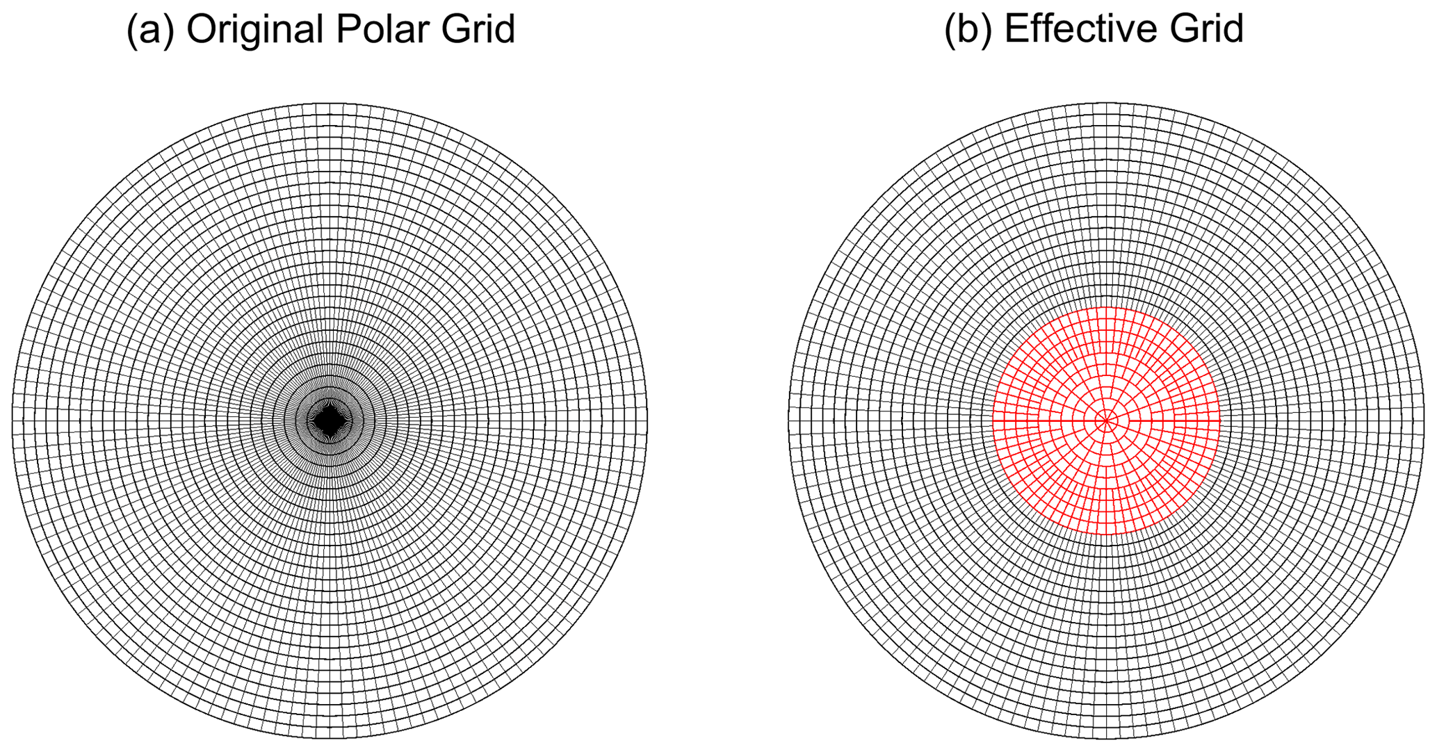
Figure 1 The (a) original and (b) effective $\mathrm{2.5}{}^{\circ }\times \mathrm{2.5}{}^{\circ }$ TIEGCM polar longitude–latitude grid. For example, the 144 azimuthal cells in the most inside (highest latitude) grid (a) have been grouped into 9 effective cells (chunks), with 16 original cells in each chunk. In the effective grid, the numbers of chunks from inside to outside are 9, 9, 18, 18, 36, 36, 72, 72, 72, and 72.

The finite-difference adaption of the ring average algorithm is based on a similar averaging–reconstruction process over a predefined “effective” azimuthal grid as used in the finite-volume version of the algorithm. Figure 1b shows an example of an effective polar grid for applying the finite-difference ring average technique. In the polar grid shown in Fig. 1b, since the reconstructed solution is monotonic within each effective computational cell, a much larger time step is allowed compared to the original grid shown in Fig. 1a. As shown in Fig. 1b, the effective longitudinal grid resolutions have been reduced and are less clustered towards the pole. For the most inside (highest latitude) grids, the 144 azimuthal cells (Fig. 1a) have been grouped into 9 effective cells (chunks), with 16 original cells in each chunk. Moving away from the pole, more chunks are employed. As an example, the numbers of chunks from inside to outside shown in Fig. 1b in the effective grid are 9, 9, 18, 18, 36, 36, 72, 72, 72, and 72, allowing a relatively smooth transition in the size of the cells going radially outward. Note that the choice of the number of chunks in each ring is non-unique. Numerical tests with finite-volume solvers have shown that the computational solution, under both smooth and discontinuous flow conditions, is insensitive to small changes in the chunk configuration (Zhang et al., 2019).

Figure 2 Schematic of grid cells within effective chunks.

We use the following example of solving the linear advection equation to illustrate the averaging–reconstruction process within each chunk. Consider the following linear advection equation of an incompressible fluid in the azimuthal direction as an example:

$$\begin{array}{}\text{(1)}& {\displaystyle \frac{\partial \mathit{\rho }}{\partial t}}+v{\displaystyle \frac{\partial \mathit{\rho }}{\partial x}}=\mathrm{0},\end{array}$$

where v is the advection velocity, ρ is the density profile, and x is the azimuthal dimension (x∈[0 2π]) along one ring. Assuming the x direction is uniformly discretized into N_total computational cells with $\mathrm{\Delta }x=\frac{\mathrm{2}\mathit{\pi }}{N_{\mathrm{total}}}$, a central-difference forward Euler form of Eq. (1) for density ρ in cell k between time n and n+1 is written as

$$\begin{array}{}\text{(2)}& {\displaystyle \frac{\mathrm{1}}{\mathrm{\Delta }t}}\left({\mathit{\rho }}_k^{n+\mathrm{1}}-{\mathit{\rho }}_k^n\right)=-{\displaystyle \frac{v}{\mathrm{2}\mathrm{\Delta }x}}\left({\mathit{\rho }}_{k+\mathrm{1}}^n-{\mathit{\rho }}_{k-\mathrm{1}}^n\right),\end{array}$$

where k denotes the index of an individual thin cell in the original azimuthal grid. Δt is the time step regulated by the CFL condition. Without a ring average type of treatment, the time step Δt is restricted by the fact that thin azimuthal cells cluster near the pole. The ring average technique takes the average solution within a chunk m that contains 2s cells in the original grid as shown in Fig. 2. Summing over the finite-difference form of Eq. (1) within chunk m gives

$$\begin{array}{}\text{(3)}& \sum _{k=i-s+\mathrm{1}}^{i+s}{\displaystyle \frac{\mathrm{1}}{\mathrm{\Delta }t}}\left({\mathit{\rho }}_k^{n+\mathrm{1}}-{\mathit{\rho }}_k^n\right)=-{\displaystyle \frac{v}{\mathrm{2}\mathrm{\Delta }x}}\sum _{k=i-s+\mathrm{1}}^{i+s}\left({\mathit{\rho }}_{k+\mathrm{1}}^n-{\mathit{\rho }}_{k-\mathrm{1}}^n\right).\end{array}$$

Then, summing over the k indices within chunk m, Eq. (3) becomes

$$\begin{array}{ll}{\displaystyle \frac{\mathrm{1}}{\mathrm{\Delta }t}}& {\displaystyle }\left(\sum _{k=i-s+\mathrm{1}}^{i+s}{\mathit{\rho }}_k^{n+\mathrm{1}}-\sum _{k=i-s+\mathrm{1}}^{i+s}{\mathit{\rho }}_k^n\right)\\ \text{(4)}& {\displaystyle }& {\displaystyle }=-{\displaystyle \frac{v}{\mathrm{2}\mathrm{\Delta }x}}\sum _{k=i-s+\mathrm{1}}^{i+s}\left[\left({\mathit{\rho }}_{k+\mathrm{1}}^n-{\mathit{\rho }}_k^n\right)+\left({\mathit{\rho }}_k^n-{\mathit{\rho }}_{k-\mathrm{1}}^n\right)\right],\text{(5)}& {\displaystyle }& {\displaystyle }=-{\displaystyle \frac{v}{\mathrm{2}\mathrm{\Delta }x}}\left[\left({\mathit{\rho }}_{i+s+\mathrm{1}}^n-{\mathit{\rho }}_{i-s+\mathrm{1}}^n\right)+\left({\mathit{\rho }}_{i+s}^n-{\mathit{\rho }}_{i-s}^n\right)\right],\text{(6)}& {\displaystyle }& {\displaystyle }=-{\displaystyle \frac{v}{\mathrm{\Delta }x}}\left({\displaystyle \frac{{\mathit{\rho }}_{i+s+\mathrm{1}}^n+{\mathit{\rho }}_{i+s}^n}{\mathrm{2}}}-{\displaystyle \frac{{\mathit{\rho }}_{i-s+\mathrm{1}}^n+{\mathit{\rho }}_{i-s}^n}{\mathrm{2}}}\right),\text{(7)}& {\displaystyle }& {\displaystyle }=-{\displaystyle \frac{v}{\mathrm{\Delta }x}}\left({\mathit{\rho }}_{i+s+\frac{\mathrm{1}}{\mathrm{2}}}^n-{\mathit{\rho }}_{i-s+\frac{\mathrm{1}}{\mathrm{2}}}^n\right),\end{array}$$

where ${\mathit{\rho }}_{i-s+\frac{\mathrm{1}}{\mathrm{2}}}^n$ and ${\mathit{\rho }}_{i+s+\frac{\mathrm{1}}{\mathrm{2}}}^n$ are the left and right values on the boundary of chunk m, as indicated by the red triangles in Fig. 2. The left-hand side of Eq. (7) is basically the time rate of the change in terms of the chunk density ϱ_m:

$$\begin{array}{}\text{(8)}& {\displaystyle \frac{\mathrm{1}}{\mathrm{\Delta }t}}\left({\mathit{\varrho }}_m^{n+\mathrm{1}}-{\mathit{\varrho }}_m^n\right),\end{array}$$

where ${\mathit{\varrho }}_m^{n+\mathrm{1}}=\sum _{k=i-s+\mathrm{1}}^{i+s}{\mathit{\rho }}_k^{n+\mathrm{1}}$ and ${\mathit{\varrho }}_m^n=\sum _{k=i-s+\mathrm{1}}^{i+s}{\mathit{\rho }}_k^n$. If assuming smoothness of the solution, which applies to typical upper-atmospheric flow conditions, and using a piecewise linear reconstruction for the two interface values at time level n,

$$\begin{array}{}\text{(9)}& {\displaystyle }& {\displaystyle }{\mathit{\rho }}_{i+s+\frac{\mathrm{1}}{\mathrm{2}}}^n={\displaystyle \frac{{\mathit{\varrho }}_{m+\mathrm{1}}+{\mathit{\varrho }}_m}{\mathrm{2}}},\text{(10)}& {\displaystyle }& {\displaystyle }{\mathit{\rho }}_{i-s+\frac{\mathrm{1}}{\mathrm{2}}}^n={\displaystyle \frac{{\mathit{\varrho }}_m+{\mathit{\varrho }}_{m-\mathrm{1}}}{\mathrm{2}}},\end{array}$$

the right-hand side of Eq. (7) is in the form of a central-difference approximation of the spatial derivative $\frac{\partial \mathit{\varrho }}{\partial x}$ in chunk m:

$$\begin{array}{}\text{(11)}& -{\displaystyle \frac{v}{\mathrm{\Delta }x}}{\displaystyle \frac{{\mathit{\varrho }}_{m+\mathrm{1}}^n-{\mathit{\varrho }}_{m-\mathrm{1}}^n}{\mathrm{2}}}.\end{array}$$

Equating Eqs. (8) and (11) and considering the fact that the ΔX in computing the chunk derivative is actually 2sΔx, we obtain

$$\begin{array}{}\text{(12)}& {\displaystyle \frac{\mathrm{1}}{\mathrm{\Delta }T}}\left({\mathit{\varrho }}_m^{n+\mathrm{1}}-{\mathit{\varrho }}_m^n\right)=-v{\displaystyle \frac{{\mathit{\varrho }}_{m+\mathrm{1}}^n-{\mathit{\varrho }}_{m-\mathrm{1}}^n}{\mathrm{2}\mathrm{\Delta }X}},\end{array}$$

where ΔT=2sΔt. Equation (12) is in the same numerical differential form of the advection equation in terms of the chunk density ϱ in the effective grid within the same order of finite-difference approximation:

$$\begin{array}{}\text{(13)}& {\displaystyle \frac{\partial \mathit{\varrho }}{\partial t}}=-v{\displaystyle \frac{\partial \mathit{\varrho }}{\partial x}}+\mathcal{O}\left(\mathrm{\Delta }{X}^{\mathrm{2}}\right).\end{array}$$

Equation (12) also suggests that in principle the ring average method is capable of using a time step that is approximately 2s times larger than the original Δt restricted by the thin cells (assuming the CFL condition is dominated by the azimuthal direction in the innermost ring). Note that the above derivation of the finite-difference version of the ring average algorithm is independent of the numerical schemes solving the linear advection equation (Eq. 1). Thus, the ring average algorithm requires no modifications to the existing hydrodynamic equations solved by GCMs. Furthermore, since the ring average algorithm is applied after all the variables are solved on the original spherical grid, it requires no changes to the existing computational grid.

In the reconstruction step, the above algorithm uses the piecewise linear method (PLM) to reconstruct solutions within each chunk for the next time step of the GCM calculations, resulting in second-order accuracy. To achieve higher accuracy in the reconstruction step, a piecewise parabolic reconstruction method (PPM) (Colella and Woodward, 1984) may be used in the algorithm, which provides fourth-order accuracy for the reconstruction step. In the following section when applying the ring average algorithm in a GCM, we use both PPM and PLM for different variables. The criteria for using PPM or PLM here depend on their spatial gradient from the fluid calculations. For variables that have a relatively greater spatial gradient, we use the PPM to reach high accuracy and maintain stability; otherwise, the PLM is used for the calculations.

The algorithm shown in Fig. 3 illustrates the steps of applying the ring average technique using either PLM or PPM. The steps consist of chunk division, chunk averaging, and reconstruction. The averaging–reconstruction process (ring average) in this study is similar to Zhang et al. (2019), with modifications to the reconstruction method (PPM or PLM) adapted to finite-difference schemes. The detailed procedures of the ring average technique in this study are described as follows.

Figure 3 The ring average algorithm with both the PLM and PPM.

2.1.1 For variables using the PLM reconstruction

• Step 1. Divide the azimuthal grid cells into chunks and pull data into the chunks.

• Step 2. Calculate the average value F_A, left interface value F_L, and right interface value F_R at chunk m (m is the index of the chunk number in an azimuthal ring). F_L and F_R are the interface values in each chunk determined by the following parabola functions:

  $$\begin{array}{}\text{(14)}& {\displaystyle }& {\displaystyle }{F}_{\mathrm{L}}=\left(-F_{m-\mathrm{2}}+\mathrm{7}{F}_{m-\mathrm{1}}+\mathrm{7}{F}_m-F_{m+\mathrm{1}}\right)/\mathrm{12},\text{(15)}& {\displaystyle }& {\displaystyle }{F}_{\mathrm{R}}=\left(-F_{m-\mathrm{1}}+\mathrm{7}{F}_m+\mathrm{7}{F}_{m+\mathrm{1}}-F_{m+\mathrm{2}}\right)/\mathrm{12},\end{array}$$

  where F_m−2, F_m−1, F_m, F_m+1, and F_m+2 are the average values F_A at chunks with an index of m−2, m−1, m, m+1, and m+2, respectively.

• Step 3. Reconstruct the variables by interpolating the average data linearly in each chunk:

  $$\begin{array}{}\text{(16)}& F_k=\left(\mathrm{1}-{\displaystyle \frac{k}{N}}\right)F_{\mathrm{L}}+{\displaystyle \frac{k}{N}}{F}_{\mathrm{R}},\end{array}$$

  where N is the number of cells within each chunk and k is the local index ranging from 1 to N.

• Step 4. Re-do the above procedures for the next azimuthal ring until the ring average is not needed.

2.1.2 For variables using the PPM reconstruction

The procedures in PPM are the same with PLM except for Step 3.

Step 3. Reconstruct the variables parabolically in each chunk using the following function:

$$\begin{array}{}\text{(17)}& F_k={\displaystyle \frac{A}{\mathrm{3}{N}^{\mathrm{2}}}}(\mathrm{3}{k}^{\mathrm{2}}-\mathrm{3}k+\mathrm{1})+{\displaystyle \frac{B}{\mathrm{2}N}}(\mathrm{2}k-\mathrm{1})+C,\end{array}$$

where A, B, and C are constants representing the parabolic function, which connects F_L and F_R:

$$\begin{array}{}\text{(18)}& \begin{array}{rl}& A=\mathrm{3}\left(F_{\mathrm{L}}-F_{\mathrm{R}}-\mathrm{2}{F}_{\mathrm{A}}\right),\\ & B=\mathrm{2}\left(\mathrm{3}{F}_{\mathrm{A}}-\mathrm{2}{F}_{\mathrm{L}}-F_{\mathrm{R}}\right),\\ & C=F_{\mathrm{L}}.\end{array}\end{array}$$

2.1.3 For vector variables using the PLM reconstruction and Fourier reduction

Step 0 in Fig. 3 corresponds to a Fourier expansion (reduction) step that is required for vector GCM variables in spherical coordinates before applying the ring average process. The main purpose of the Fourier reduction step is to maintain the direction of vectors after ring averaging, especially for the neutral meridional and zonal wind across the pole. Thus, only the second and higher Fourier components of the data in the azimuthal cell are smoothed using the ring average filter, while the zero and first Fourier components are kept unchanged. Here are the details of the Fourier expansion process.

Step 0. Calculate the Fourier components of the azimuthal data:

$$\begin{array}{}\text{(19)}& P_i=A_{\mathrm{0}}+A_{\mathrm{1}}\cos \left(\mathrm{2}\mathit{\pi }i/N_{\mathrm{total}}\right)+B_{\mathrm{1}}\sin \left(\mathrm{2}\mathit{\pi }i/N_{\mathrm{total}}\right)+F_i,\end{array}$$

where i is the thin cell index along the azimuthal direction ranging from 1 to N_total, N_total is the total thin cell number in the azimuthal direction, F_i represents the second and higher Fourier components that will be later reconstructed, and A₀, A₁, and B₁ are the zero and first Fourier coefficients:

$$\begin{array}{}\text{(20)}& \begin{array}{rl}& A_{\mathrm{0}}={\displaystyle \frac{\mathrm{1}}{L}}\sum _{i=\mathrm{1}}^{i=L}{P}_i,\\ & A_{\mathrm{1}}={\displaystyle \frac{\mathrm{1}}{L}}\sum _{i=\mathrm{1}}^{i=L}{P}_i\cos (\mathrm{2}\mathit{\pi }i/L),\\ & B_{\mathrm{1}}={\displaystyle \frac{\mathrm{2}}{L}}\sum _{i=\mathrm{1}}^{i=L}{P}_i\sin (\mathrm{2}\mathit{\pi }i/L).\end{array}\end{array}$$

The higher Fourier components F_i are pulled into chunks for the ring average processes.

Step 1–4. The steps are the same as the above PLMs, except that the reconstructed data, $F_i^{\prime }$, are brought back together with the first two Fourier components after the reconstruction:

$$\begin{array}{}\text{(21)}& P_i=A_{\mathrm{0}}+A_{\mathrm{1}}\cos (\mathrm{2}\mathit{\pi }i/L)+B_{\mathrm{1}}\sin (\mathrm{2}\mathit{\pi }i/L)+F_i^{\prime }.\end{array}$$

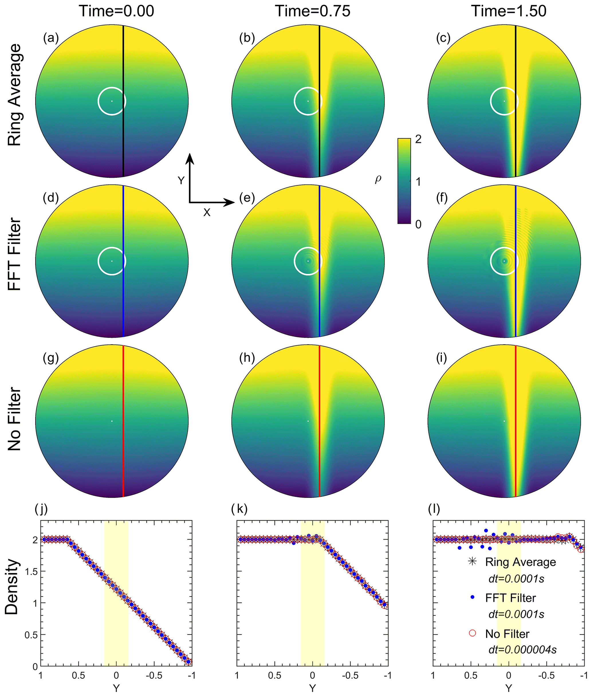
Figure 4 The distribution of density at three simulation snapshots (t=0, 0.75, and 1.5). The first three panels from the top show the results with the ring average technique, with an FFT filter, and without any filter. The latitude boundaries of the ring average and FFT filter are marked by white circles in the upper two panels. The bottom panels show the comparison of distributions of density along the line x=0.15 (star) with the ring average technique, (blue dot) with an FFT filter, and (red circle) without a filter at the three snapshots. The number of averaging chunks for the ring average technique in each azimuthal ring near the pole is set to be [18 18 18 18 36 36 36 36 72 72 72 72 144 144 144 144].

2.2 Ring average for the advection equation

In this section, in order to illustrate the implementation of the ring average algorithm in a finite-difference code, we solve the two-dimensional (2D) linear advection equation in the polar geometry as an example. The code used in the 2D linear advection solver is a main subroutine used in the ring average module for GCMs. This two-dimensional advection test in polar geometry is also useful to demonstrate the effectiveness of the finite-difference ring average technique in handling a strong, narrow shear flow near the pole. A fourth-order central-finite-difference scheme is used to solve the following mass continuity equation under the incompressible assumption:

$$\begin{array}{}\text{(22)}& {\displaystyle \frac{\partial \mathit{\rho }}{\partial t}}+\mathit{u}\cdot \mathrm{\nabla }\mathit{\rho }=\mathrm{0},\end{array}$$

where ρ is the density, and u is the time-stationary flow velocity defined in polar coordinates (r, θ). The polar geometry of this test is defined with a resolution of 0.625^∘ in both longitude and latitude, with 144 cells in the r direction uniformly distributed within (0, 1) and 576 cells in the θ direction uniformly distributed within (0, 2π).

Figure 4a shows the initial state (t=0) of ρ, ranging linearly along the y direction from a magnitude of 2 at the topside to 0.01 at the bottom side:

$$\begin{array}{}\text{(23)}& \mathit{\rho }=\left\{\begin{array}{ll}\mathrm{2}& y\ge \mathrm{0.65}\\ (y-\mathrm{0.65})/(\mathrm{0.65}+\mathrm{1})\cdot (\mathrm{2}-\mathrm{0.01})+\mathrm{2}& y<\mathrm{0.65}\end{array}\right..\end{array}$$

The time-independent flow velocity u is set as a Gaussian-distributed shear flow towards −y and centered at x=0.15 with a peak velocity of −1 and a half-width of 0.01:

$$\begin{array}{}\text{(24)}& u=-\exp \left[-{\displaystyle \frac{(x-\mathrm{0.15}{)}^{\mathrm{2}}}{\mathrm{0.01}}}\right].\end{array}$$

As simulation time evolves, a large density gradient occurs near the pole driven by the time-stationary shear flow, with its pattern following the analytical distribution of the flow velocity u. Figure 4a–c show three snapshots of the density in the linear advection experiment at t=0, t=0.75, and t=1.5 using the finite-difference version of the ring average technique with PPM reconstructions, as described in Sect. 2.1. For comparison, Fig. 4d–f show the corresponding snapshots derived from another simulation using an FFT filter, and Fig. 4g–i show the results at the same simulation time calculated from the fourth-order finite-difference scheme without applying any filtering technique. In the simulation using the ring average, the number of averaging chunks in each azimuthal ring near the pole is set to be [18 18 18 18 36 36 36 36 72 72 72 72 144 144 144 144] from the first ring to the 16th ring, as indicated by the white circles in the top panels around 80^∘ N. For the FFT filter, a Fourier expansion is applied in the azimuthal direction at each time step to the fluid density. Waves with frequencies that are higher than the cutoff frequencies are eliminated from the Fourier spectra of prognostic variables. The values of prognostic variables are then reconstructed through an inverse Fourier transform using the modified Fourier spectra. Each latitude grid has its own cutoff frequency, and the wave number to be cut off in this experiment near the pole is set to be [1 1 2 2 2 2 4 4 4 4 8 8 8 8 10 10], which is similar to the TIEGCM FFT filter spectrum (Wang, 1998).

As shown in Fig. 4b and c, density structures with a large spatial gradient flow across the pole as time progresses. Compared with the non-filter case in Fig. 4h and i, no evident numerical instability or artificial structure occurred when applying the ring average technique. In contrast, the density structure using an FFT filter in Fig. 4d–f exhibits numerical oscillations in the radial direction, together with an artificial depletion of density near the pole. This density depletion is due to the non-conservative nature of the FFT method by truncating high-spatial-frequency wave modes in a linear way. Figure 4j–l show a one-dimensional comparison of the density profiles along x=0.15, with the region of averaging chunks denoted by yellow. The comparisons suggest that the density flow is not noticeably affected by the implementation of the ring average technique in the finite-difference solver. Note that the time step used after applying the ring average technique is 0.0001 s, which is 25 times larger than that used in the simulation without the ring average (dt=0.000004 s). Although the FFT filter can result in non-oscillatory solutions in the finite-difference solver, as shown by the one-dimensional profiles in Fig. 4l, evident density oscillations occur near the pole due to numerical instability caused by the FFT method. The cutoff frequency of the FFT filter is case-dependent and has a problem of mass loss compared to the ring average method. The advection experiment illustrates that the ring average technique is capable of relaxing the severe time step constraint and resolving large density gradients when passing through the clustered grid cells near the pole.

2.3 Ring average for GCMs

We use the NCAR TIEGCM to demonstrate the effectiveness of the ring average technique in resolving mesoscale upper-atmospheric structures. TIEGCM is a physics-based 3D global model that solves the coupled equations of momentum, energy, and continuity for neutral and ion species in the upper-atmospheric I–T system using a fourth-order and centered finite-difference scheme to evolve the advection terms on each pressure surface with a staggered vertical grid (Qian et al., 2014; Roble et al., 1988; Richmond et al., 1992). The TIEGCM utilizes a spherical coordinate system fixed with respect to the rotating Earth, with geographic latitude and longitude as the horizontal coordinates and the pressure surface as the vertical coordinate. The following is a brief introduction of the basic equations in the TIEGCM.

The thermospheric energy equation is

$$\begin{array}{}\text{(25)}& \begin{array}{rl}{\displaystyle \frac{\partial T_n}{\partial t}}& =-\mathbf{U}\cdot \mathit{▿}{T}_n+{\displaystyle \frac{g{e}^Z}{P_{\mathrm{0}}{C}_{\mathrm{p}}}}{\displaystyle \frac{\partial }{\partial Z}}\left\{{\displaystyle \frac{K_{\mathrm{T}}}{H}}{\displaystyle \frac{\partial T_n}{\partial Z}}\right.\\ & \left.+K_{\mathrm{E}}{H}^{\mathrm{2}}{C}_{\mathrm{P}}\mathit{\rho }\left[{\displaystyle \frac{g}{C_{\mathrm{P}}}}+{\displaystyle \frac{\mathrm{1}}{H}}{\displaystyle \frac{\partial T_n}{\partial Z}}\right]\right\}\\ & -w\left({\displaystyle \frac{\partial T_n}{\partial Z}}+{\displaystyle \frac{R^{*}T}{C_{\mathrm{p}}\stackrel{\mathrm{‾}}{m}}}\right)+{\displaystyle \frac{Q-L}{C_{\mathrm{P}}}},\end{array}\end{array}$$

with temperature T_n, time t, the vertical coordinate $Z=\ln (P_{\mathrm{0}}/P)$, the pressure P, and the reference pressure P₀; g is gravity, K_T is the molecular thermal conductivity, C_P is the specific heat per unit mass, H is the pressure scale height, K_E is the eddy diffusion coefficient, ρ is the atmospheric mass density, U is the horizontal neutral velocity with the zonal and meridional components u_n and v_n, w is the vertical velocity defined by $w=\mathrm{d}Z/\mathrm{d}t$, R^* is the universal gas constant, $\stackrel{\mathrm{‾}}{m}$ is the mean atmospheric mass, and Q and L are the heating and cooling rates. The mean molecular mass $\stackrel{\mathrm{‾}}{m}$ is determined by

$$\begin{array}{}\text{(26)}& \stackrel{\mathrm{‾}}{m}=\left[{\displaystyle \frac{{\mathrm{\Psi }}_{{\mathrm{O}}_{\mathrm{2}}}}{m_{{\mathrm{O}}_{\mathrm{2}}}}}+{\displaystyle \frac{{\mathrm{\Psi }}_{\mathrm{O}}}{m_{\mathrm{O}}}}+{\displaystyle \frac{{\mathrm{\Psi }}_{{\mathrm{N}}_{\mathrm{2}}}}{m_{{\mathrm{N}}_{\mathrm{2}}}}}\right],\end{array}$$

where Ψ and m represent the mass mixing ratio and the molecular mass, respectively, for the three thermospheric major species O₂, O, and N₂.

The zonal momentum equation is expressed as

$$\begin{array}{}\text{(27)}& \begin{array}{rl}{\displaystyle \frac{\partial u_n}{\partial t}}& =-\mathbf{U}\cdot \mathit{▿}{u}_n+{\displaystyle \frac{g{e}^Z}{P_{\mathrm{0}}}}{\displaystyle \frac{\partial }{\partial Z}}\left({\displaystyle \frac{\mathit{\mu }}{H}}{\displaystyle \frac{\partial u_n}{\partial Z}}\right)\\ & +\left(f+{\displaystyle \frac{u_n}{R_{\mathrm{E}}}}\tan \mathit{\lambda }\right)v_n+{\mathit{\lambda }}_{xx}\left(u_i-u_n\right)\\ & +{\mathit{\lambda }}_{xy}\left(v_i-v_n\right)-w{\displaystyle \frac{\partial u_n}{\partial Z}}-{\displaystyle \frac{\mathrm{1}}{R_{\mathrm{E}}\cos \mathit{\lambda }}}{\displaystyle \frac{\partial \mathit{\varphi }}{\partial \mathit{\phi }}},\end{array}\end{array}$$

and the meridional momentum equation is

$$\begin{array}{}\text{(28)}& \begin{array}{rl}{\displaystyle \frac{\partial v_n}{\partial t}}& =-\mathbf{U}\cdot \mathit{▿}{v}_n+{\displaystyle \frac{g{e}^Z}{P_{\mathrm{0}}}}{\displaystyle \frac{\partial }{\partial Z}}\left({\displaystyle \frac{\mathit{\mu }}{H}}{\displaystyle \frac{\partial v_{\mathrm{n}}}{\partial Z}}\right)\\ & -\left(f+{\displaystyle \frac{u_{\mathrm{n}}}{R_{\mathrm{E}}}}\tan \mathit{\lambda }\right)u_{\mathrm{n}}+{\mathit{\lambda }}_{yy}\left(v_i-v_{\mathrm{n}}\right)\\ & +{\mathit{\lambda }}_{yx}\left(u_i-u_{\mathrm{n}}\right)-w{\displaystyle \frac{\partial v_{\mathrm{n}}}{\partial Z}}-{\displaystyle \frac{\mathrm{1}}{R_{\mathrm{E}}}}{\displaystyle \frac{\partial \mathit{\varphi }}{\partial \mathit{\lambda }}},\end{array}\end{array}$$

where λ and φ represent the geographic latitude and longitude, respectively. R_E is the radius of the Earth, μ is the viscosity coefficient, which is the sum of eddy and molecular viscosity coefficients, f is the Coriolis parameter, ϕ is the geopotential, H is the pressure scale height, v_i and u_i are the meridional and zonal E×B ion drift velocities, and λ_xx, λ_xy, λ_yx, and λ_yy are the ion-drag tensor coefficients. The TIEGCM “vertical velocity” $w=\mathrm{d}Z/\mathrm{d}t$ is determined by solving the continuity equation:

$$\begin{array}{}\text{(29)}& {\displaystyle \frac{\mathrm{1}}{R_{\mathrm{E}}\cos \mathit{\lambda }}}{\displaystyle \frac{\partial }{\partial \mathit{\lambda }}}\left(v_n\cos \mathit{\lambda }\right)+{\displaystyle \frac{\mathrm{1}}{R_{\mathrm{E}}\cos \mathit{\lambda }}}{\displaystyle \frac{\partial u_n}{\partial \mathit{\phi }}}+e^Z{\displaystyle \frac{\partial }{\partial Z}}\left(e^{-Z}w\right)=\mathrm{0}.\end{array}$$

The real vertical velocity is obtained by first integrating the continuity equation (Eq. 29) over Z to get w and then multiplying w by the neutral pressure scale height to get the right unit.

The thermospheric major species in the TIEGCM include O₂, O, and N₂. The continuity equation for the mass mixing ratio of O₂ and O is given by

$$\begin{array}{}\text{(30)}& \begin{array}{rl}{\displaystyle \frac{\partial \stackrel{\mathrm{̃}}{\mathrm{\Psi }}}{\partial t}}& =-\mathbf{U}\cdot \mathit{▿}\stackrel{\mathrm{̃}}{\mathrm{\Psi }}-{\displaystyle \frac{e^Z}{\mathit{\tau }}}{\displaystyle \frac{\partial }{\partial Z}}\left[{\displaystyle \frac{\stackrel{\mathrm{‾}}{m}}{m_{{\mathrm{N}}_{\mathrm{2}}}}}{\left({\displaystyle \frac{T_{\mathrm{00}}}{T_n}}\right)}^{\mathrm{0.25}}{\stackrel{\mathrm{̃}}{\mathit{\alpha }}}^{-\mathrm{1}}L\stackrel{\mathrm{̃}}{\mathrm{\Psi }}\right]\\ & +e^Z{\displaystyle \frac{\partial }{\partial Z}}\left[K\left(Z\right)e^{-Z}{\displaystyle \frac{\partial }{\partial Z}}\left(\mathrm{1}+{\displaystyle \frac{\mathrm{1}}{\stackrel{\mathrm{‾}}{m}}}{\displaystyle \frac{\partial \stackrel{\mathrm{‾}}{m}}{\partial Z}}\right)\stackrel{\mathrm{̃}}{\mathrm{\Psi }}\right]\\ & +\stackrel{\mathrm{̃}}{S}-\stackrel{\mathrm{̃}}{R}-w{\displaystyle \frac{\partial \stackrel{\mathrm{̃}}{\mathrm{\Psi }}}{\partial Z}},\end{array}\end{array}$$

where $\stackrel{\mathrm{̃}}{\mathrm{\Psi }}=({\mathrm{\Psi }}_{{\mathrm{O}}_{\mathrm{2}}}$, Ψ_O), τ is the diffusion timescale equal to 1.86×10³ s, $m_{{\mathrm{N}}_{\mathrm{2}}}$ is the molecular mass for molecular nitrogen, T₀₀=273 K is the standard temperature, $\stackrel{\mathrm{̃}}{\mathit{\alpha }}$ is the matrix operator of the diffusion coefficients, K(Z) is the eddy diffusion coefficient, and $\stackrel{\mathrm{̃}}{S}$ and $\stackrel{\mathrm{̃}}{R}$ are the production and loss terms for these two species. The diagonal matrix operator L has elements of the form

$$\begin{array}{}\text{(31)}& {\displaystyle }{L}_{ii}={\displaystyle \frac{\partial }{\partial Z}}-\left(\mathrm{1}-{\displaystyle \frac{m_i}{\stackrel{\mathrm{‾}}{m}}}-{\displaystyle \frac{\mathrm{1}}{\stackrel{\mathrm{‾}}{m}}}{\displaystyle \frac{\partial \stackrel{\mathrm{‾}}{m}}{\partial Z}}\right),\end{array}$$

where i=1 and i=2 denote O₂ and O, respectively. The N₂ mass mixing ratio is determined by

$$\begin{array}{}\text{(32)}& {\mathrm{\Psi }}_{{\mathrm{N}}_{\mathrm{2}}}=\mathrm{1}-{\mathrm{\Psi }}_{{\mathrm{O}}_{\mathrm{2}}}-{\mathrm{\Psi }}_{\mathrm{O}}.\end{array}$$

The minor species in the TIEGCM are N(⁴S), N(²D), and NO. The timescale of N(⁴S) is relatively short and is thus considered to be in photochemical equilibrium. N(⁴S) and NO have longer lifetimes, so the transport effects must be taken into account. The governing equation for these two species is

$$\begin{array}{}\text{(33)}& \begin{array}{rl}{\displaystyle \frac{\partial \stackrel{\mathrm{̃}}{\mathrm{\Psi }}}{\partial t}}& =-\mathbf{U}\cdot \mathit{▿}\stackrel{\mathrm{̃}}{\mathrm{\Psi }}-e^Z{\displaystyle \frac{\partial }{\partial Z}}\left[\stackrel{\mathrm{̃}}{A}\left({\displaystyle \frac{\partial }{\partial Z}}-\stackrel{\mathrm{̃}}{E}\right)\stackrel{\mathrm{̃}}{\mathrm{\Psi }}\right]\\ & +e^Z{\displaystyle \frac{\partial }{\partial Z}}\left[e^{-Z}{K}_{\mathrm{E}}\left(Z\right)\left({\displaystyle \frac{\partial }{\partial Z}}+{\displaystyle \frac{\mathrm{1}}{\stackrel{\mathrm{‾}}{m}}}{\displaystyle \frac{\partial \stackrel{\mathrm{‾}}{m}}{\partial Z}}\right)\stackrel{\mathrm{̃}}{\mathrm{\Psi }}\right]\\ & -w{\displaystyle \frac{\partial \stackrel{\mathrm{̃}}{\mathrm{\Psi }}}{\partial Z}}+\stackrel{\mathrm{̃}}{S}-\stackrel{\mathrm{̃}}{R},\end{array}\end{array}$$

where

$$\begin{array}{}\text{(34)}& \stackrel{\mathrm{̃}}{E}=\left(\mathrm{1}-{\displaystyle \frac{m}{\stackrel{\mathrm{‾}}{m}}}-{\displaystyle \frac{\mathrm{1}}{\stackrel{\mathrm{‾}}{m}}}{\displaystyle \frac{\partial \stackrel{\mathrm{‾}}{m}}{\partial Z}}\right)-\stackrel{\mathrm{̃}}{\mathit{\alpha }}{\displaystyle \frac{\mathrm{1}}{T_n}}{\displaystyle \frac{\partial T_n}{\partial Z}}+\stackrel{\mathrm{̃}}{F}\stackrel{\mathrm{̃}}{\mathrm{\Psi }},\end{array}$$

where $\stackrel{\mathrm{̃}}{\mathrm{\Psi }}=({\mathrm{\Psi }}_{\mathrm{NO}}$, ${\mathrm{\Psi }}_{\mathrm{N}{(}^{\mathrm{4}}\mathrm{S})})$, $\stackrel{\mathrm{̃}}{A}$ is the vertical molecular diffusion coefficient, and $\stackrel{\mathrm{̃}}{S}$ and $\stackrel{\mathrm{̃}}{R}$ are the production and loss terms for each species. Terms in $\stackrel{\mathrm{̃}}{E}$ represent the effects of gravity, thermal diffusion, and the frictional interaction with the major species on the vertical profiles of these two species. $\stackrel{\mathrm{̃}}{F}$ is a matrix operator for the frictional interactions, $\stackrel{\mathrm{̃}}{\mathit{\alpha }}$ is the thermal diffusion coefficient, and $\stackrel{\mathrm{̃}}{m}$ is the molecular mass for the two minor species.

The ions of the ionosphere in the TIEGCM include O⁺, ${\mathrm{O}}_{\mathrm{2}}^{+}$, NO⁺, N⁺, and ${\mathrm{N}}_{\mathrm{2}}^{+}$, and the electron density is calculated by chemical equilibrium of these ions. All major ionospheric ions except O⁺ are assumed to be in photochemical equilibrium; thus, their densities can be calculated simply by balancing the loss and production rates. The O⁺ density is determined not only by O⁺ loss and production but also by transport due to E×B drifts, neutral winds, and field-aligned ambipolar diffusion. The O⁺ continuity equation can be expressed as

$$\begin{array}{}\text{(35)}& {\displaystyle \frac{\partial n}{\partial t}}=-\mathit{▿}\cdot \left(n\mathbf{V}\right)+Q-Ln,\end{array}$$

where n is the O⁺ density, Q is the production rate, L is the loss rate, and ▿⋅(nV) is the transport term. The ion velocity V is given by

$$\begin{array}{}\text{(36)}& {\displaystyle }& {\displaystyle }\mathbf{V}={\mathbf{V}}_{\Vert }+{\mathbf{V}}_{⟂},\text{(37)}& {\displaystyle }& {\displaystyle }{\mathbf{V}}_{\Vert }=\left\{\mathit{b}\cdot {\displaystyle \frac{\mathrm{1}}{{\mathit{\nu }}_{\mathrm{in}}}}\left[\mathit{g}-{\displaystyle \frac{\mathrm{1}}{{\mathit{\rho }}_{\mathrm{i}}}}\mathit{▿}\left(P_{\mathrm{i}}+P_{\mathrm{e}}\right)\right]+\mathit{b}\cdot {\mathbf{U}}_{\mathrm{n}}\right\}\mathit{b},\text{(38)}& {\displaystyle }& {\displaystyle }{\mathbf{V}}_{⟂}={\displaystyle \frac{\mathbf{E}\times \mathbf{B}}{|\mathbf{B}{|}^{\mathrm{2}}}},\end{array}$$

where V_‖ (caused by ambipolar diffusion and neutral winds) and V_⟂ (caused by E×B drifts) are the parallel and perpendicular velocities with respect to the magnetic field line, respectively, b is a unit vector along the magnetic field, ν_in is the ion-neutral collision frequency, g is the acceleration due to gravity, ρ_i is the ion mass density, P_i and P_e are the ion and electron pressures, respectively, U_n is the neutral velocity, B is the magnetic field, and E is the electric field.

By assuming a thermal quasi-steady state, the electron energy equation is

$$\begin{array}{}\text{(39)}& {\sin }^{\mathrm{2}}I{\displaystyle \frac{\partial }{H\partial Z}}\left(K^{\mathrm{e}}{\displaystyle \frac{\partial T_{\mathrm{e}}}{H\partial Z}}\right)+\sum Q_{\mathrm{e}}-\sum L_{\mathrm{e}}=\mathrm{0},\end{array}$$

with I the geomagnetic dip angle, K^e the electron thermal conductivity parallel to the magnetic field, ∑Q_e the sum of all local electron heating rates, and ∑L_e the sum of all local cooling rates.

Figure 5 The main ring average algorithm in the TIEGCM.

For the electrodynamics, i.e., the “neutral wind dynamo process”, TIEGCM assumes steady-state electrodynamics with a divergence-free current density J for longer timescales:

$$\begin{array}{}\text{(40)}& \begin{array}{rl}\mathit{▿}& \cdot \left[{\mathit{\sigma }}_{\mathrm{P}}\mathit{b}\times \left(\mathbf{E}+{\mathbf{U}}_{\mathrm{n}}\times \mathbf{B}\right)\times \mathit{b}+{\mathit{\sigma }}_{\mathrm{H}}\mathit{b}\times \left(\mathbf{E}+{\mathbf{U}}_{\mathrm{n}}\times \mathbf{B}\right)\right.\\ & \left.+{\mathbf{J}}_{\left|\right|}+{\mathbf{J}}_{\mathrm{M}}\right]=\mathrm{0},\end{array}\end{array}$$

where σ_P and σ_H are the Pedersen and Hall conductivities, respectively. ${\mathbf{J}}_{\left|\right|}$ and J_M are the ohmic component of current density parallel to the magnetic field and the non-ohmic magnetospheric component, respectively.

The ionospheric convection pattern for computing the plasma advection velocity V_⟂ at high latitudes is specified by either the Heelis et al. (1982) or the Weimer (2005) empirical model, while at the bottom boundary the migrating tides are specified using the Global Scale Wave Model (Hagan and Forbes, 2002, 2003). The current standard version of TIEGCM (TIEGCM v2.0) provides two spatial resolution options: (1) $\mathrm{5}{}^{\circ }\times \mathrm{5}{}^{\circ }$ in horizontal geographic latitude–longitude grid and $\mathrm{1}/\mathrm{2}$ scale height in the vertical direction or (2) $\mathrm{2.5}{}^{\circ }\times \mathrm{2.5}{}^{\circ }$ in horizontal geographic latitude–longitude grid and $\mathrm{1}/\mathrm{4}$ scale height in the vertical direction.

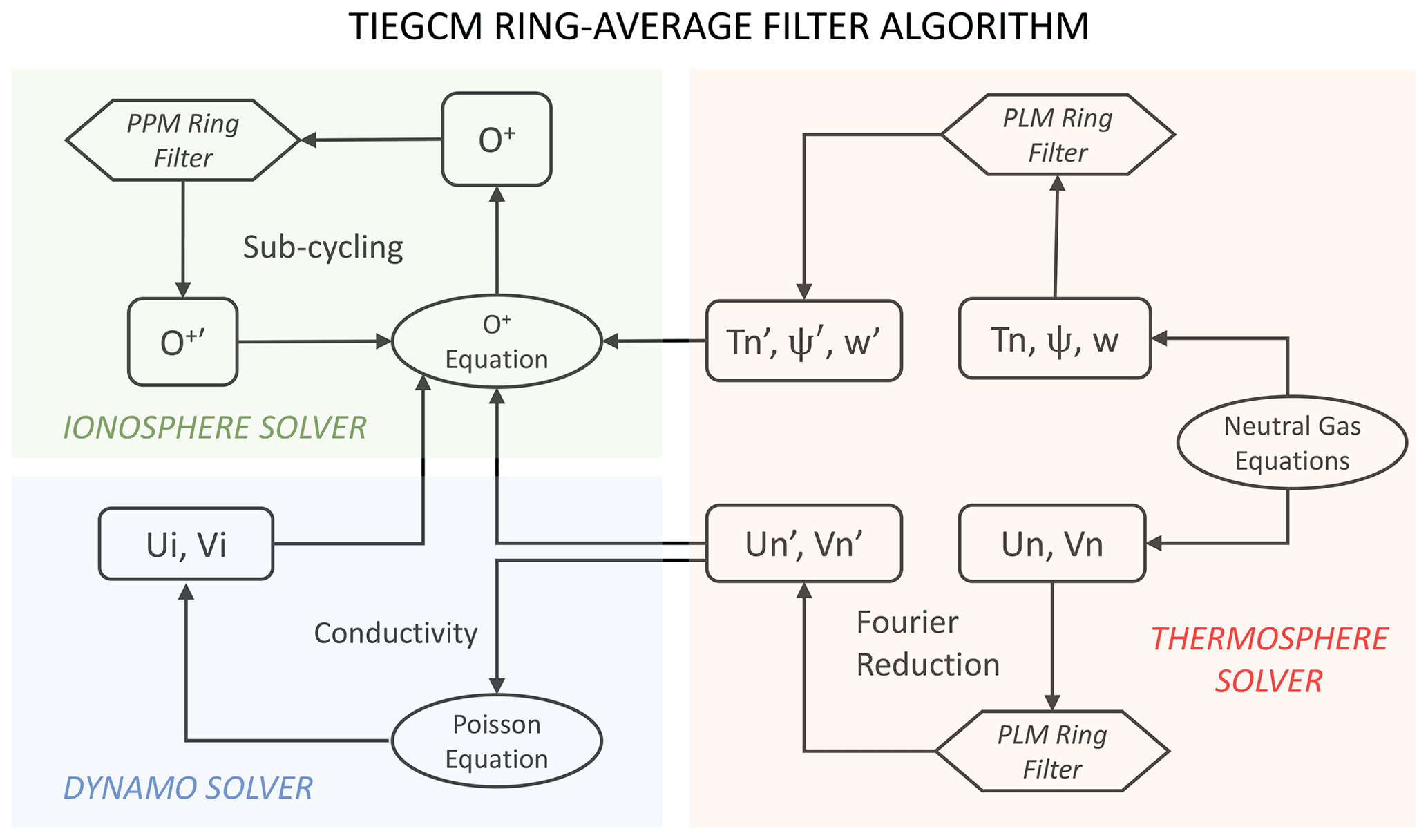
In this study, the ring average technique is implemented in the TIEGCM v2.0 to solve the issue of clustering grid cells near the poles in the development of a high-resolution version of the TIEGCM. This technique is applied as a post-processing treatment of the fluid variables including oxygen ion density O⁺, neutral temperature T_n, thermospheric compositions Ψ, and meridional, zonal, and vertical winds (U_n, V_n, w) at each time step, with different reconstruction methods (PPM or PLM) for different variables (Table 1). Due to the use of MPI parallelization in the TIEGCM in supercomputers, the ring average technique firstly collects the azimuthal data in the root thread, conducts the averaging–reconstruction process, and finally redistributes data into each MPI thread. Figure 5 illustrates ring average filters used in the main algorithms of the TIEGCM, including the thermosphere solvers in Equations (25)–(34), the ionosphere solver for O⁺ in Eqs. (35)–(39), and the dynamo solver for electrodynamic coupling in the Eq. (40). For neutral variables in the thermosphere solver, the ring average technique with the PLM reconstruction is utilized. Specifically, for the meridional and zonal neutral winds, the second and higher Fourier components are processed with the PLM ring average filter to maintain the direction of vectors across the pole, as displayed in Fig. 5. The oxygen ion (O⁺) in the ionosphere usually has much sharper gradients than the neutral variables, e.g., tongue of ionization (TOI) structures; thus, the PPM is used in the reconstruction process to provide high-order accuracy and handle the larger local gradient. Meanwhile, to balance the numerical stability and computational speed, a sub-cycling technique, which has a smaller time step for O⁺ than neutral variables, has been applied in the O⁺ solver because the ions can move much faster than the neutrals with the E×B drifts, especially during major geomagnetic storms.

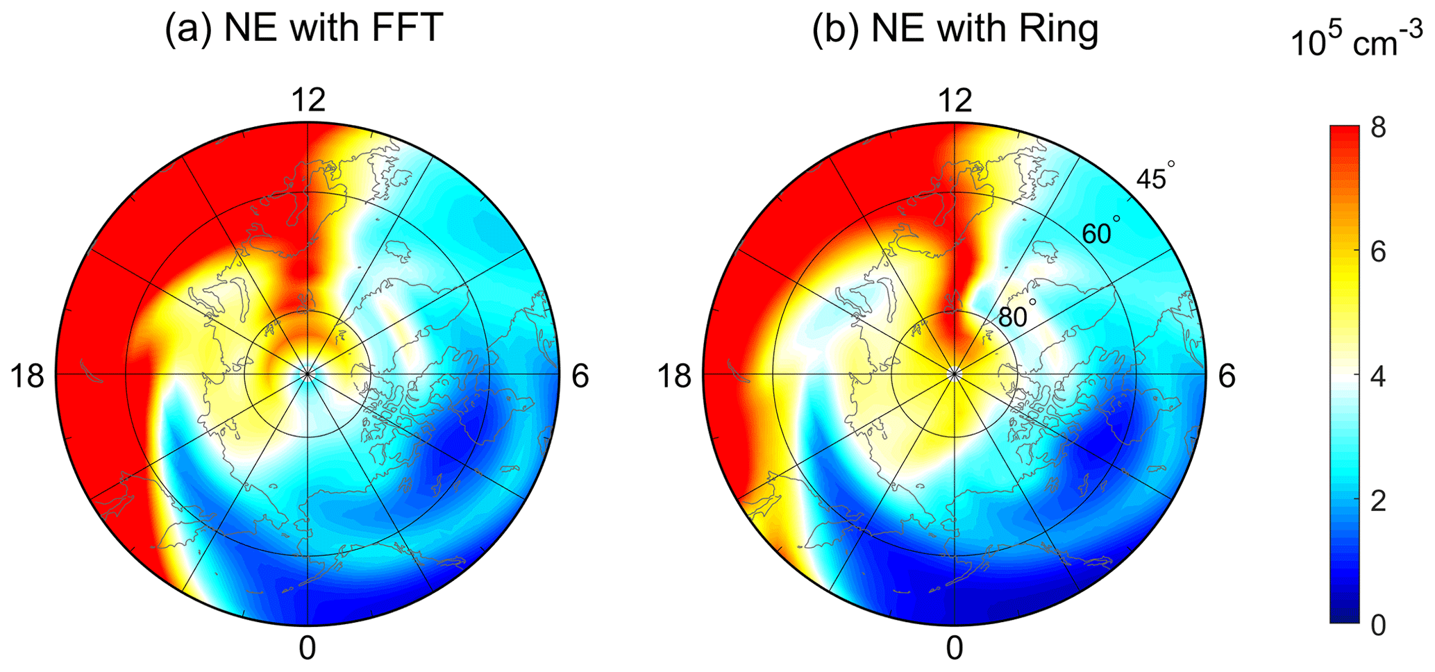
Figure 6 The simulated polar maps of electron densities using (a) an FFT filter and (b) ring average at pressure surface 2 (near the F₂-region peak, ∼300 km) at 10:50 UT on 17 March 2013 as a function of geographic latitude and local time. Both simulations have a horizontal resolution of $\mathrm{2.5}{}^{\circ }\times \mathrm{2.5}{}^{\circ }$. The outer boundary is at 45^∘ N geographic latitude.

On the basis of the ring average technique, a new high-resolution version of TIEGCM with a horizontal longitude–latitude resolution as high as $\mathrm{0.625}{}^{\circ }\times \mathrm{0.625}{}^{\circ }$ is developed. Table 2 lists the ring average setup used in different TIEGCM resolutions. The third column in Table 2 represents the number of averaging chunks in each azimuthal ring near the pole from the first innermost to the outermost rings. For example, in the first azimuthal ring near the pole of the $\mathrm{0.625}{}^{\circ }\times \mathrm{0.625}{}^{\circ }$ grid resolution, 64 longitude grids ($\mathrm{576}/\mathrm{9}=\mathrm{64}$) and 40 longitude degrees ($\mathrm{360}{}^{\circ }/\mathrm{9}=\mathrm{40}{}^{\circ }$) are grouped into a chunk. In the outermost filtered ring (around 71.25^∘ latitude), one averaging chunk only contains two longitude grids. Table 3 summarizes the information on different spatial resolutions of the TIEGCM, including the current version of the $\mathrm{2.5}{}^{\circ }\times \mathrm{2.5}{}^{\circ }$ TIEGCM with the default FFT filter and the $\mathrm{2.5}{}^{\circ }\times \mathrm{2.5}{}^{\circ }$, $\mathrm{1.25}{}^{\circ }\times \mathrm{1.25}{}^{\circ }$, and $\mathrm{0.625}{}^{\circ }\times \mathrm{0.625}{}^{\circ }$ resolution TIEGCM with the ring average filter. As the resolution doubles, the time step decreases approximately linearly rather than quadratically. In practice, the $\mathrm{0.625}{}^{\circ }\times \mathrm{0.625}{}^{\circ }$ resolution of the code runs about 2 times faster than real time with 256 processors on the NCAR/CISL Cheyenne supercomputer system (12 h for a 1 d geomagnetic storm simulation), which is at fairly low computational cost for mesoscale-resolving global simulations. The preliminary results of the high-resolution TIEGCM will be shown in the following section.

Table 1 The basic ring average settings of variables (column 1) and the corresponding reconstruction method (column 2), Fourier reduction (column 3), and sub-cycling (column 4) in the TIEGCM.

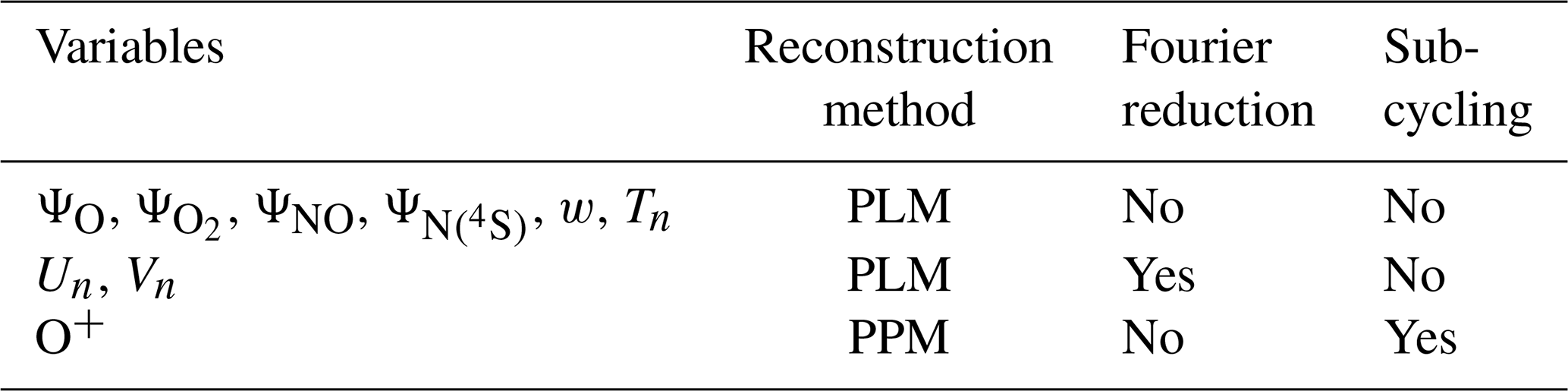
Table 2 The ring average setup for different TIEGCM horizontal resolutions (column 1) associated with the number of longitude grids (column 2) and the number of averaging chunks in each azimuthal ring near the pole (column 3).

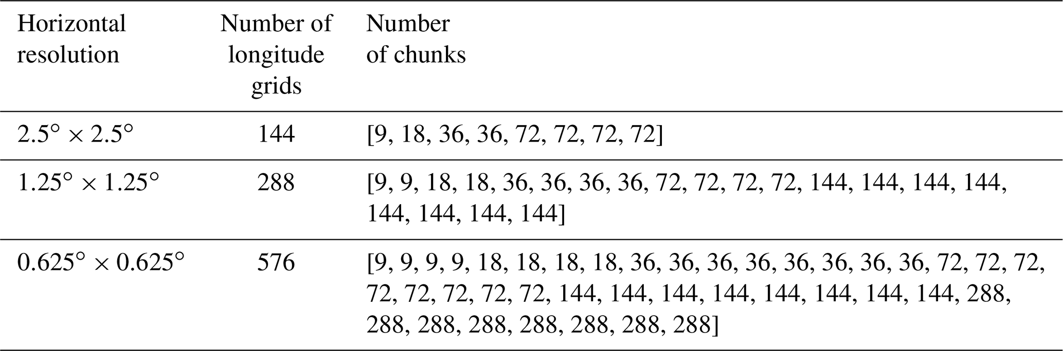
Table 3 Comparisons of horizontal resolution in a geographic latitude–longitude grid (column 1), vertical resolution (column 2), time step (column 3), O⁺ sub-cycling time step (column 4), and polar filter (column 5) between different TIEGCM versions^*.

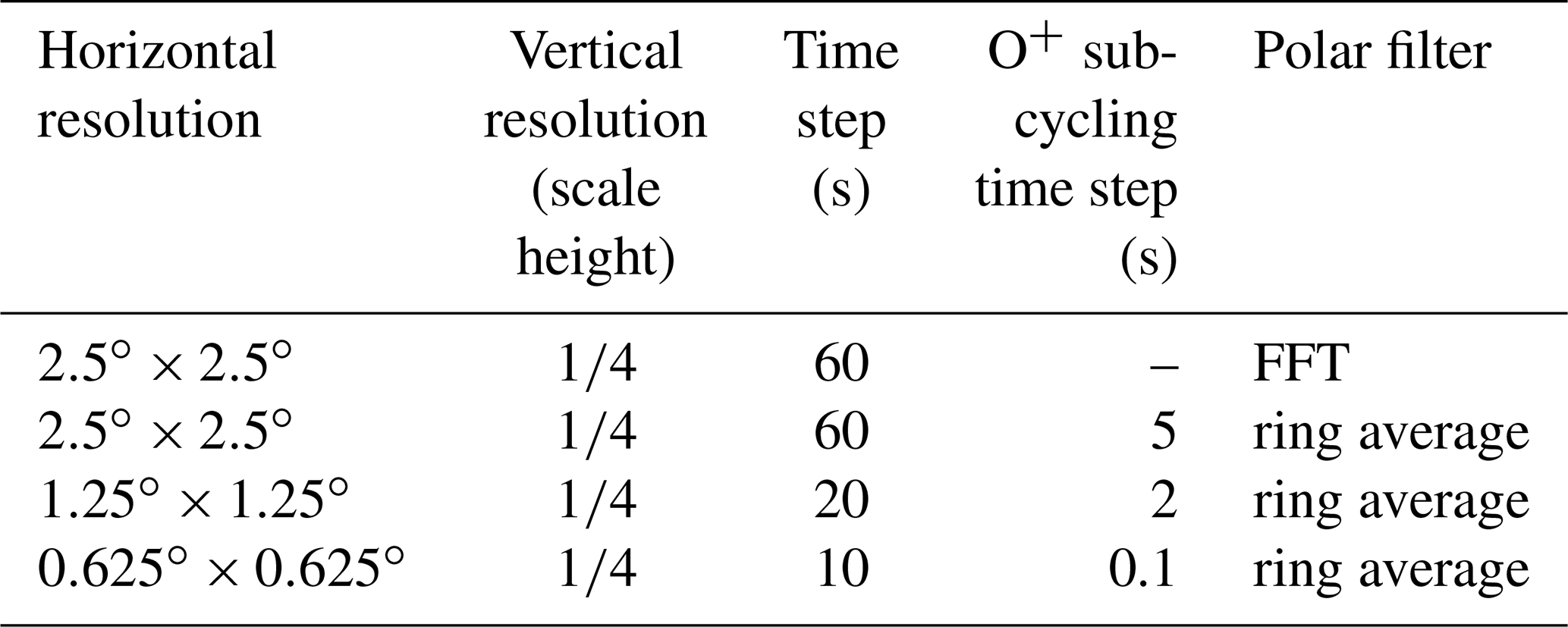
^* In columns 3 and 4, the time step corresponds to the cases of geomagnetic storms. The time step and sub-cycling time step would be more relaxed when the geomagnetic activity is quiet.

3 Applications

To show the capability of the new high-resolution TIEGCM based on the ring average technique in resolving mesoscale I–T structures, we have simulated the ionospheric and thermospheric variations during the 17 March 2013 major geomagnetic storm as an example. Figure 6 displays the comparison of polar maps of electron densities between different filter techniques with the $\mathrm{2.5}{}^{\circ }\times \mathrm{2.5}{}^{\circ }$ horizontal resolution. The electron density is plotted on pressure surface 2, which is near the F₂-region peak (∼300 km of altitude). Figure 6a corresponds to the standard TIEGCM with the FFT filter, while Fig. 6b is the result using the ring average technique. Generally, the electron densities in the two simulations in Fig. 6a and b are similar below 60^∘ N, with an evident electron density enhancement seen in the afternoon sector and negative storm effects in the morning at 10:50 UT during the storm. The dense ionospheric plasma in the afternoon sector is transported in the anti-sunward direction into the polar cap region by the dusk cell of the convection pattern. Consequently, prominent polar tongue of ionization (TOI) features can be seen as a narrow density plume on the dayside, which stretches from 65^∘ N at noon to latitudes greater than 80^∘ N inside the polar cap. Those TOI features agree well with the polar Global Position System (GPS) total electron content (TEC) observations (e.g., Foster et al., 2005; Thomas et al., 2013). It is evident that, in Fig. 6a, the TOI cannot go through the polar cap region and generates an artificial “hole” structure above 80^∘ N. This nonphysical depletion is associated with the loss of electron density induced by the removal of high frequency in the FFT filter, as also indicated in the advection experiment in Fig. 4f. Consequently, the plasma within the TOI accumulates around the hole and a “ring-like” structure appears at about 70^∘ N. In contrast, for the ring average technique, the electron densities in Fig. 6b can successfully flow through the polar cap and arrive at the nightside, which is consistent with Fig. 4c. Thus, using the ring average, the artificial structures no longer exist in the polar cap region, indicating the advantage of the ring average technique in handling numerical instability by causing fewer artificial structures and preserving the real mesoscale structures.

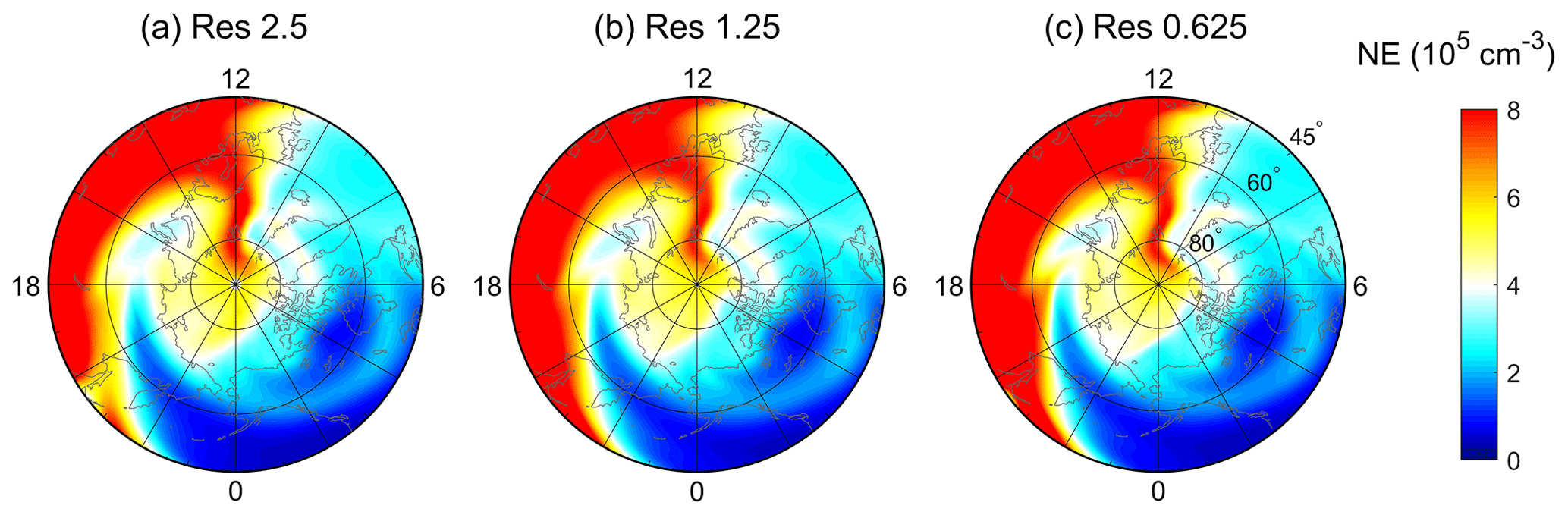
Figure 7 The polar maps of electron densities at pressure surface 2 (near the F₂-region peak, ∼300 km) at 10:50 UT on 17 March 2013 as a function of geographic latitude and local time for (a) $\mathrm{2.5}{}^{\circ }\times \mathrm{2.5}{}^{\circ }$, (b) $\mathrm{1.25}{}^{\circ }\times \mathrm{1.25}{}^{\circ }$, and (c) $\mathrm{0.625}{}^{\circ }\times \mathrm{0.625}{}^{\circ }$ TIEGCM horizontal resolutions using the ring average technique.

Figure 7 shows the comparison of the polar maps of electron densities between simulations with different spatial resolutions using the TIEGCM bolstered by the ring average technique. The simulation results after using the ring average technique are generally similar among different simulations, with finer structures at higher spatial resolutions. Besides the ionospheric parameters, we have also tested the performance of the ring average in thermospheric simulations (not shown here), which indicates that the thermospheric variables generally converge between different spatial resolutions. The thermospheric temperature, $\mathrm{O}/{\mathrm{N}}_{\mathrm{2}}$, and thermospheric density simulated by two kinds of filters do not show distinct differences compared with the ionospheric simulations due to the relatively smoother variations of neutral parameters. Only slight deviation exists locally on a smaller scale in the polar thermosphere. The results from Figs. 6 and 7 demonstrate that the ring average technique can be applied in the finite-difference method, which is usually considered to be less stable than the finite-volume scheme. The ring average method can successfully maintain numerical stability, even with the structures of large spatial gradients, and conserve true mesoscale structures. Meanwhile, the ring average technique shows advantages of inexpensive computational cost and easy implementation, as indicated by Table 3. By using the ring average, the time step has been greatly relaxed in the ideal advection experiment and the high-resolution TIEGCM, which would maintain the computational cost at an acceptable level. Furthermore, ring averaging can be applied as a post-filter after each simulation step and would not require a modification of the underlying code; this would make the technique easily applied.

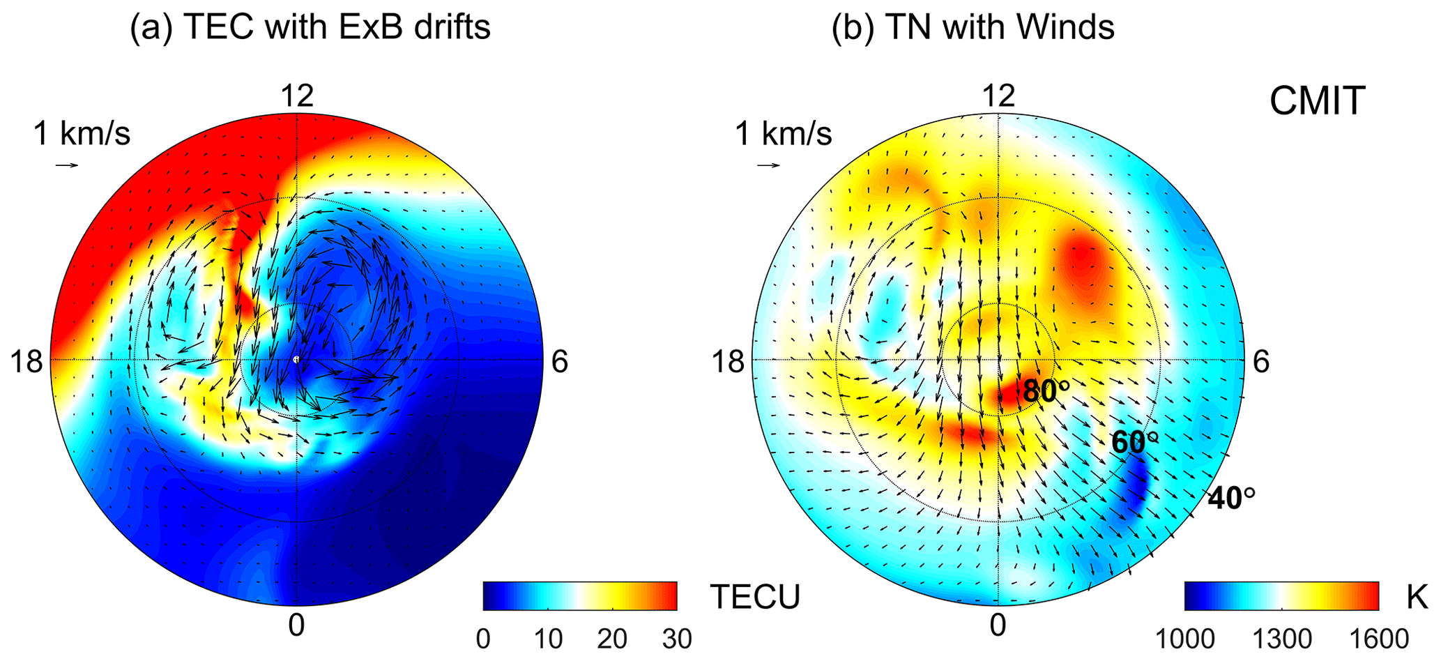
Figure 8 Polar maps of the (a) total electron content (TEC) and (b) neutral temperature simulated by CMIT as a function of geographic latitude and local time at 17:30 UT on 17 March 2013. The vectors represent the (a) E×B drifts and (b) horizontal neutral winds.

Benefiting from the ring average technique, the newly developed high-resolution TIEGCM has been applied to explore the mesoscale variations in the I–T system during space weather events. For instance, based on the $\mathrm{0.625}{}^{\circ }\times \mathrm{0.625}{}^{\circ }$ high-resolution TIEGCM simulations and satellite observations, Dang et al. (2019) reported the occurrence of double TOIs and carried out a comprehensive study on the dynamic evolution and formation mechanism of double TOIs. Lu et al. (2020) used the high-resolution model to study ionospheric disturbances such as traveling ionospheric disturbances and enhanced storm density during geomagnetic disturbances. The high-resolution TIEGCM has also been utilized to simulate the sub-auroral polarization stream (Lin et al., 2019), neutral wind variabilities (Wu et al., 2019), and the responses of the I–T system to solar eclipses (Dang et al., 2018a, b; Lei et al., 2018; Wang et al., 2019). These works highlight the enhanced capability of the high-resolution TIEGCM in resolving ionospheric and thermospheric mesoscale structures enabled by the ring average technique.

Simulating the mesoscale structures also requires a more realistic input from the upper boundary, corresponding to the electric field and auroral precipitation from the magnetosphere, and the bottom boundary, corresponding to the upward propagation of tides and waves from the lower atmosphere, of the I–T system. In the TIEGCM, these inputs are directly adopted from two empirical models, the Weimer model and the Global Scale Wave Model (GSWM), which might not necessarily represent the complexity of the actual physical processes from the boundaries. To obtain a more physical upper boundary condition, the CMIT has been developed (Wang et al., 2004; Wiltberger et al., 2004), which couples the LFM global magnetosphere model with the I–T model TIEGCM. The LFM provides the TIEGCM with high-latitude electric fields and auroral electron precipitation, and the TIEGCM feeds ionospheric height-integrated conductance back to the LFM. The standard resolution of the ionosphere and thermosphere in CMIT is $\mathrm{2.5}{}^{\circ }\times \mathrm{2.5}{}^{\circ }$, which is the same as the standard TIEGCM. By implementing the high-resolution TIEGCM in CMIT, the thermosphere–ionosphere part in CMIT has a horizontal resolution of 1.25^∘ in both latitude and longitude, which is comparable to the magnetospheric resolution of 100 km mapped to the ionospheric reference altitude. Figure 8 shows an example CMIT simulation of the ionosphere and thermosphere at 17:30 UT during the 17 March 2013 geomagnetic storm. The TEC in Fig. 8a shows more dynamic and finer TOI variations driven by the magnetospheric convection during the storm time. Meanwhile, the thermospheric temperature in Fig. 8b also exhibits distinct mesoscale structures associated with changes in the neutral wind circulation and ion collisional heating. The results illustrate that, with the implementation of the ring average technique, the high-resolution CMIT show advantages in resolving the dynamic evolution of mesoscale structures in the coupled magnetosphere–ionosphere–thermosphere system.

Furthermore, the ring average technique has also been applied in the WACCM-X, which can provide a relatively more realistic bottom boundary for the I–T simulation. The WACCM-X is a whole-atmosphere chemistry–climate general circulation model spanning the range of altitude from the Earth's surface to the upper thermosphere to simulate the entire atmosphere and ionosphere (Liu et al., 2018). The ionosphere and electrodynamo parts in WACCM-X are the same as in the TIEGCM. The ring average scheme has been successfully implemented in the O⁺ transport module of the WACCM-X to get a higher spatial resolution for the ionosphere. Figure 9 shows the simulation results for the 17 March 2013 geomagnetic storm from WACCM-X. For this simulation, the horizontal resolution is $\mathrm{1.25}{}^{\circ }\times \mathrm{0.9}{}^{\circ }$ in longitude and latitude directions, respectively, and the vertical resolution in the upper atmosphere is $\mathrm{1}/\mathrm{4}$ of the scale height. Detailed analyses and exploration of the CMIT and WACCM-X results are beyond the scope of this study and will be studied in the future. Ongoing efforts also include improving the resolution of the vertical direction and the electrodynamo of the TIEGCM as well as applying the ring average technique to high-resolution data assimilation and space weather prediction.

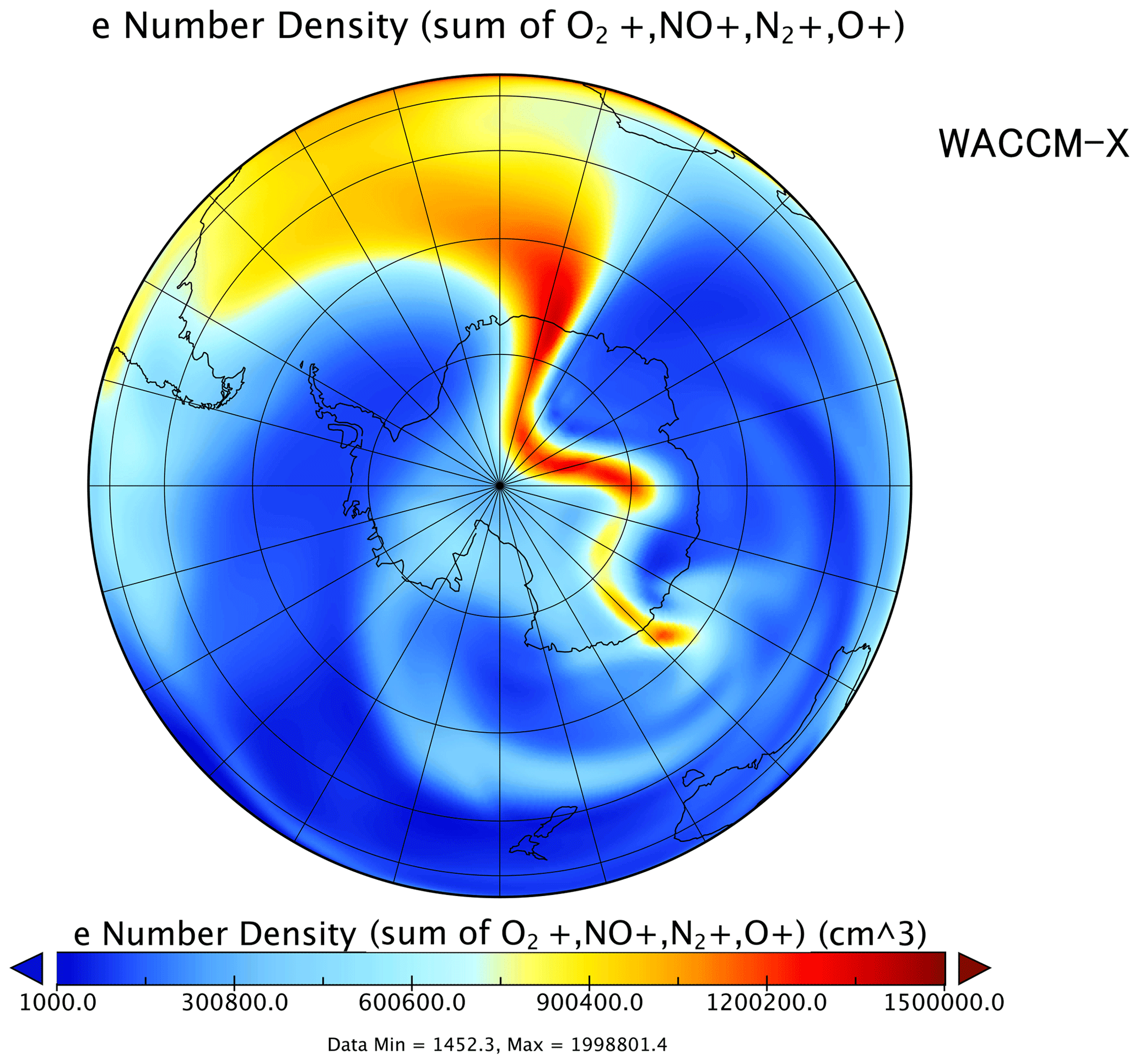
Figure 9 Polar map of the electron density in the Southern Hemisphere at 14:00 UT on 17 March 2013 from the WACCM-X 1^∘ simulation.

4 Summary

In summary, a post-processing technique with an averaging–reconstruction (ring average) algorithm is developed to solve the problem of clustering of azimuthal cells in a spherical coordinate with the finite-difference method. The ring average technique is applied based on a reduced effective polar grid by first averaging quantities within azimuthal effective “chunks” and then reconstructing them within each chunk. The ring average technique shows the advantages of inexpensive computational cost, easy implementation, time step relaxation, and maintenance of the mesoscale structures without introducing artifacts, which allows for the development of high-resolution GCMs to resolve mesoscale structures. We have developed a new version of the TIEGCM, which has a horizontal resolution of $\mathrm{0.625}{}^{\circ }\times \mathrm{0.625}{}^{\circ }$ in a geographic longitude–latitude grid, by implementing the ring average technique as a post-processing step. The nonphysical “hole” and “ring” structures, which are induced by an FFT filter in the previous TIEGCM version, no longer exist in the high-resolution TIEGCM associated with the ring average technique. The simulation results illustrate that the high-resolution TIEGCM is capable of resolving the mesoscale structures in the I–T system during a geomagnetic storm event. Moreover, the ring average scheme has also been implemented in CMIT and WACCM-X to enable high-spatial-resolution self-consistent simulations of the whole geospace from the ground to the magnetosphere.