the Creative Commons Attribution 4.0 License.
the Creative Commons Attribution 4.0 License.
 | 09 Jul 2021
Recalibrating decadal climate predictions – what is an adequate model for the drift?
Alexander Pasternack
Jens Grieger
Henning W. Rust
Uwe Ulbrich
Near-term climate predictions such as multi-year to decadal forecasts are increasingly being used to guide adaptation measures and building of resilience. To ensure the utility of multi-member probabilistic predictions, inherent systematic errors of the prediction system must be corrected or at least reduced. In this context, decadal climate predictions have further characteristic features, such as the long-term horizon, the lead-time-dependent systematic errors (drift) and the errors in the representation of long-term changes and variability. These features are compounded by small ensemble sizes to describe forecast uncertainty and a relatively short period for which typical pairs of hindcasts and observations are available to estimate calibration parameters. With DeFoReSt (Decadal Climate Forecast Recalibration Strategy), Pasternack et al. (2018) proposed a parametric post-processing approach to tackle these problems. The original approach of DeFoReSt assumes third-order polynomials in lead time to capture conditional and unconditional biases, second order for dispersion and first order for start time dependency. In this study, we propose not to restrict orders a priori but use a systematic model selection strategy to obtain model orders from the data based on non-homogeneous boosting. The introduced boosted recalibration estimates the coefficients of the statistical model, while the most relevant predictors are selected automatically by keeping the coefficients of the less important predictors to zero. Through toy model simulations with differently constructed systematic errors, we show the advantages of boosted recalibration over DeFoReSt. Finally, we apply boosted recalibration and DeFoReSt to decadal surface temperature forecasts from the German initiative Mittelfristige Klimaprognosen (MiKlip) prototype system. We show that boosted recalibration performs equally as well as DeFoReSt and yet offers a greater flexibility.
- Article
(3610 KB) - Full-text XML
- BibTeX
- EndNote


Decadal climate predictions of initialized forecasts focus on describing the climate variability for the coming years. Significant advances have been made by recent progress in model development, data assimilation for initialization and climate observation. A need for up-to-date and reliable near-term climate information and services for adaptation and planning accompanies this progress (e.g., Meredith et al., 2018). In this context, international (e.g., DCPP, Decadal Climate Prediction Project WCRP: World Climate Research Programme, and WCRP Grand Challenge on Near-Term Climate Prediction) and national projects like the German initiative Mittelfristige Klimaprognosen (MiKlip) have developed model systems to produce skillful decadal ensemble climate prediction (Pohlmann et al., 2013; Marotzke et al., 2016). Typically, ensemble climate predictions are framed probabilistically to address the inherent uncertainties caused by imperfectly known initial conditions and model errors (Palmer et al., 2006).
Despite the progress being made in decadal climate forecasting, such forecasts still suffer from considerable systematic errors like unconditional and conditional biases and ensemble over- or underdispersion. Those errors generally depend on forecast lead time since models tend to drift from the initial state towards its own climatology (Fučkar et al., 2014; Maraun, 2016). Furthermore, there can be a dependency on initialization time when long-term trends of the forecast system and observations differ (Kharin et al., 2012). In this regard, Pasternack et al. (2018) proposed a Decadal Forecast Recalibration Strategy (DeFoReSt) which accounts for the three above-mentioned systematic errors. While DCPP recommends to calculate and adjust model bias for each lead time separately to take the drift into account, Pasternack et al. (2018) uses a parametric approach to describe systematic errors as a function of lead time.
DeFoReSt uses third-order polynomials in lead time to capture conditional and unconditional biases, second-order polynomials for dispersion and a first-order polynomial to model initialization time dependency. Third-order polynomials for the drift have been suggested by Gangstø et al. (2013) and have later been used by Kruschke et al. (2015).
Hence, DeFoReSt is an extension of the drift correction approach proposed by Kruschke et al. (2015), accounting also for conditional bias and adjusting the ensemble spread.
The associated DeFoReSt parameters are estimated by minimization of the CRPS, analogous to the nonhomogeneous Gaussian regression approach by Gneiting et al. (2005).
Although DeFoReSt with third- and/or second-order polynomials turned out in past applications to be beneficial for both full-field initialized decadal predictions (Pasternack et al., 2018) and anomaly initialized counterparts (Paxian et al., 2018), as well as decadal regional predictions (Feldmann et al., 2019), it is worth challenging the a priori assumption by using a systematic model selection strategy. In this context, full-field initializations show larger drifts in comparison to anomaly initializations even though drift of the latter is not negligible, particularly when taking initialization time dependency into account (Kruschke et al., 2015).
For post-processing of probabilistic forecasts with non-homogeneous Gaussian regression, Messner et al. (2017) proposed the non-homogeneous boosting to automatically select the most relevant predictors. Originally, boosting has been developed for automatic statistical classification (Freund and Schapire, 1997) but has been used as well for statistical regression (e.g., Friedman et al., 2000; Bühlmann and Yu, 2003; Bühlmann and Hothorn, 2007).
Unlike other parameter estimation strategies based on iterative minimization of a cost function by simultaneously updating the full set of parameters, boosting only updates one parameter at a time: the one that leads to the largest decrease in the cost function. As all parameters are initialized to zero, those parameters corresponding to terms which do not lead to a considerable decrease in the cost function – hence are not relevant – will not be updated and thus will not differ from zero; the associated term has thus no influence on the predictor. Here, we extend the underlying non-homogeneous regression model of DeFoReSt to higher-order polynomials and use boosting for parameter estimation. Additionally, cross-validation identifies the optimal number of boosting iteration and serves thus for model selection. The resulting boosted non-homogeneous regression model is hereafter named boosted recalibration.
A toy model producing synthetic decadal forecast–observation pairs is used to study the effect of using higher-order polynomials and boosting on recalibration. Moreover, we compare boosted recalibration and DeFoReSt to recalibrate forecasts from the MiKlip decadal prediction system.
The paper is organized as follows: Sect. 2 introduces the MiKlip decadal climate prediction system and the corresponding reference data used, Sect. 3 describes the decadal forecast recalibration strategy DeFoReSt and introduces boosted recalibration, an extension to higher-order polynomials, parameter estimation with non-homogeneous boosting and cross-validation for model selection. A toy model developed in Sect. 4 is the basis for assessing recalibration with boosted recalibration and DeFoReSt. The subsequent section (Sect. 5) uses both approaches to recalibrate decadal surface temperature predictions from the MiKlip system. Analogously to Pasternack et al. (2018), we assess the forecast skill of global mean surface temperature and temperature over the North Atlantic subpolar gyre region (50–65∘ N, 60–10∘ W). The latter has been identified as a key region for decadal climate predictions (e.g., Pohlmann et al., 2009; van Oldenborgh et al., 2010; Matei et al., 2012; Mueller et al., 2012). Section 6 closes with a discussion.
2.1 Decadal climate forecasts
The basis for this study is retrospective forecast (hereafter called hindcast) of surface temperature from the Max Planck Institute Earth System Model in a low-resolution configuration (MPI-ESM-LR). The atmospheric component of the coupled model is ECHAM6 at a horizontal resolution of T63 with 47 vertical levels up to 0.01 hPa (Stevens et al., 2013). The ocean component is the Max Planck Institute ocean model (MPIOM) with a nominal resolution of 1.5∘ and 40 vertical levels (Jungclaus et al., 2013). This setup together with a full-field initialization of the atmosphere with ERA40 (Uppala et al., 2005) and ERA-Interim (Dee et al., 2011), as well as a full-field initialization of the ocean with the GECCO2 reanalysis (Köhl, 2015), is called the MiKlip prototype system. The full-field initialization nudges the full atmospheric or oceanic fields from the corresponding reanalysis to the MPI-ESM, not just the anomalies. A detailed description of the prototype system is given in Kröger et al. (2018). In the following, we use a hindcast set from the MiKlip prototype system with 50 hindcasts, each with 10 ensemble members integrated for 10 years starting every year in the period 1961 to 2010.
2.2 Reference data
The Met Office Hadley Centre and the Climatic Research Unit at the University of East Anglia produced HadCRUT4 (Morice et al., 2012), an observational product used here as a reference to verify the decadal hindcasts. The historical surface temperature anomalies with respect to the reference period 1961–1990 are available on a global 5∘ × 5∘ grid on a monthly basis since January 1850. HadCRUT4 is a composite of the CRUTEM4 (Jones et al., 2012) land-surface air temperature dataset and the HadSST3 (Brohan et al., 2006) sea-surface temperature (SST) dataset.
2.3 Assessing reliability and sharpness
To assess the performance of boosted recalibration with respect to DeFoReSt, we use the same metrics as in Pasternack et al. (2018).
Calibration or reliability refers to the statistical consistency between the forecast probability distributions and the verifying observations (Jolliffe and Stephenson, 2012). A forecast is reliable if forecast probabilities correspond to observed frequencies on average. Alternatively, a necessary condition for forecasts to be reliable is given if the time mean intra-ensemble variance equals the mean squared error (MSE) between ensemble mean and observation (Palmer et al., 2006).
A common tool to evaluate the reliability and therefore the effect of a recalibration is the rank histogram or Talagrand diagram which was separately proposed by Anderson (1996); Talagrand et al. (1997); Hamill and Colucci (1997). For a detailed understanding, the rank histogram has to be evaluated by visual inspection. Analog to Pasternack et al. (2018), we use the ensemble spread score (ESS) as a summarizing measure. The ESS is the ratio between the time mean intra-ensemble variance and the mean squared error between ensemble mean and observation, MSE(μ,y) (Palmer et al., 2006; Keller and Hense, 2011):
with
and
Here, and yj are the ensemble variance, the ensemble mean and the corresponding observation at time step j, with , where k is the number of time steps.
Following Palmer et al. (2006), ESS=1 indicates perfect reliability. The forecast is overconfident when ESS<1; i.e., the ensemble spread underestimates forecast error. If the ensemble spread is greater than the model error (ESS>1), the forecast is overdispersive and the forecast spread overestimates forecast error. To better understand the components of the ESS, we also analyze the MSE of the forecast separately.
Sharpness, on the other hand, refers to the concentration or spread of a probabilistic forecast and is a property of the forecast only. A forecast is sharp when it is taking a risk, i.e., when it is frequently different from the climatology. The smaller the forecast spread, the sharper the forecast. Sharpness is indicative of forecast performance for calibrated and thus reliable forecasts, as forecast uncertainty reduces with increasing sharpness (subject to calibration). To assess sharpness, we use properties of the width of prediction intervals as in Gneiting and Raftery (2007). Analogously to Pasternack et al. (2018), we use the time mean intra-ensemble variance to assess the prediction width.
Scoring rules, like the continuous ranked probability score (CRPS), assign numerical scores to probabilistic forecasts and form attractive summary measures of predictive performance, since they address reliability and sharpness simultaneously (Gneiting et al., 2005; Gneiting and Raftery, 2007; Gneiting and Katzfusss, 2014).
Given that F is the predictive probability distribution function and Fo denotes the Heaviside function for the verifying observations o with Fo(y)=1 for y>o and Fo(y)=0 otherwise, the CRPS is defined as
Under the assumption that the predictive distribution F is a normal distribution with mean μ and variance σ2, Gneiting et al. (2005) showed that Eq. (4) can be written as
where and denote the probability distribution function (CDF) and the probability density function (PDF), respectively, of the standard normal distribution. The CRPS is negatively oriented. A lower CRPS indicates more accurate forecasts; a CRPS of zero denotes a perfect (deterministic) forecast.
Its skill score (CRPSS) relates the accuracy of the prediction system to the accuracy of a reference prediction (e.g., climatology). Thus, with hindcast scores CRPSF and reference scores CRPSR, the CRPSS can be defined as
Positive values of the CRPSS imply that the prediction system outperforms the reference prediction. Furthermore, this skill score is unbounded for negative values (because hindcasts can be arbitrarily bad) but bounded by 1 for a perfect forecast.
We first review the decadal climate forecast recalibration strategy (DeFoReSt) proposed by Pasternack et al. (2018) and illustrate subsequently how a modeling strategy based on boosting and cross-validation leads to an optimal selection of polynomial orders in the non-homogeneous regression model used for recalibration.
3.1 Review of DeFoReSt
DeFoReSt assumes normality for the PDF for a predicted variable X for each initialization time and lead time . thus describes the recalibrated forecast PDF of a given variable X or – expressed in terms of the ensemble – the distribution of the recalibrated ensemble members around the recalibrated ensemble mean as a function of initialization time t and forecast lead year τ. Mean μ𝙲𝚊𝚕(t,τ) and variance of the recalibrated PDF are now modeled as linear functions of the ensemble mean and ensemble variance as
Note that, different from Pasternack et al. (2018), the logarithm in Eq. (8) ensures positive recalibrated variance irrespectively of the value of γ. Hence, the recalibrated X𝙲𝚊𝚕 is now conceived as a random variable:
α(t,τ) accounts for the (unconditional) bias depending on lead year (i.e., the drift). Similarly, β(t,τ) accounts for the conditional bias. Thus, the expectation of the recalibrated variable can be conceived as a conditional and unconditional bias and drift-adjusted ensemble mean forecast. Moreover, DeFoReSt assumes that the ensemble spread σ(t,τ) is sufficiently well related to the forecast uncertainty such that adequate adjustment can be realized by multiplying γ(t,τ). Figure 1 shows a schematic which shows the mechanisms of DeFoReSt for an exemplary decadal forecast which exhibits a lead- and start-time-dependent unconditional bias, conditional bias and dispersion.
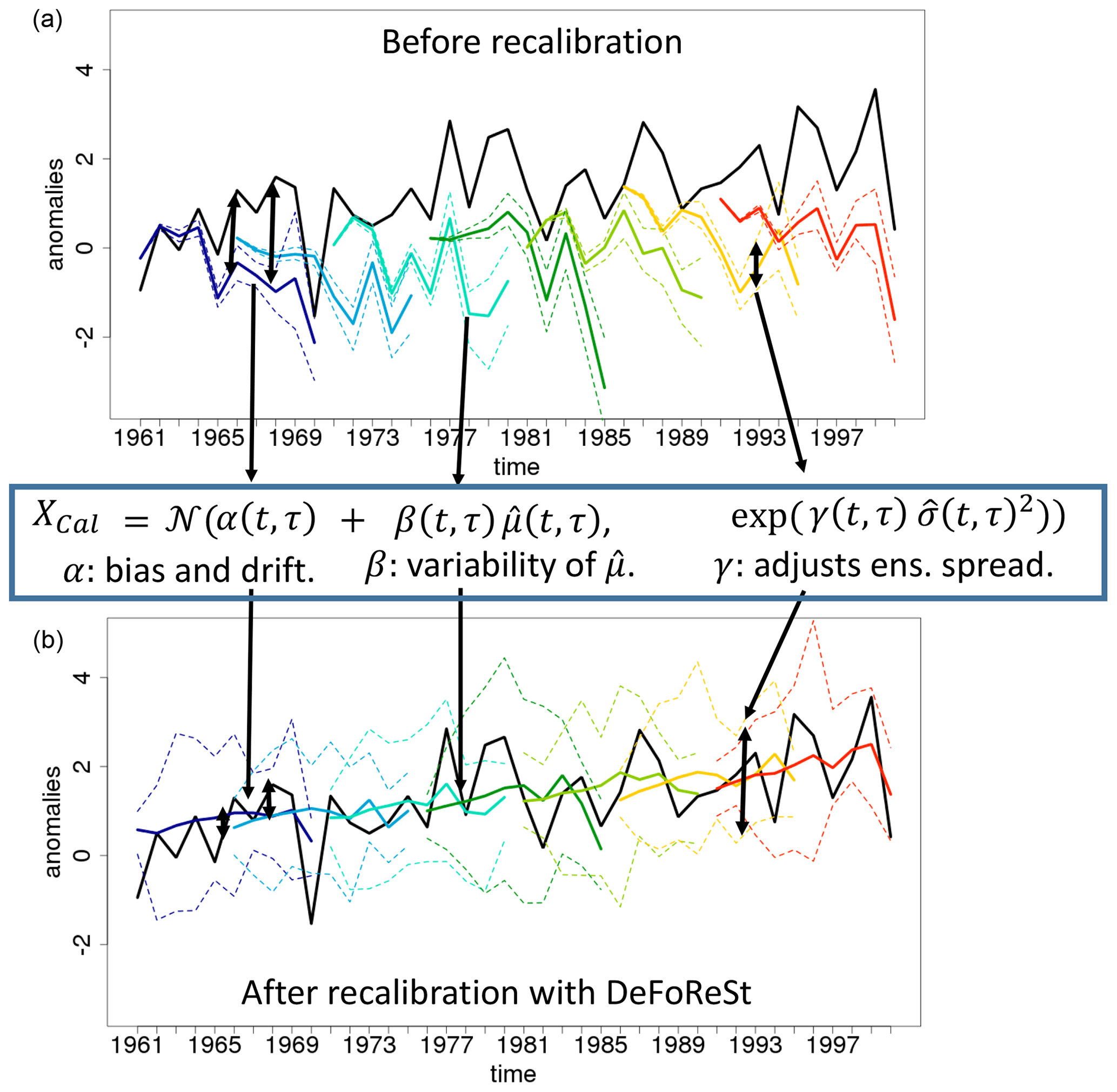
Figure 1Schematic overview of the effect of DeFoReSt for an exemplary decadal toy model with ensemble mean (colored lines), ensemble minimum/maximum (colored dotted lines) and associated pseudo-observations (black line). Note that different colors indicate different initialization times. Before recalibration (a), the ensemble mean shows a lead-time-dependent mean or unconditional bias (drift) which is tackled by α(t,τ). Moreover, the ensemble mean exhibits a conditional bias, i.e., that the variances of and observations disagree. This is tackled with β(t,τ). Decadal predictions can also be over- or underdispersive, i.e., that the ensemble spread over- or underestimates the error between observations and ensemble mean. This example shows an overdispersive forecast. Within DeFoReSt, the coefficient γ(t,τ) accounts for the dispersiveness of the forecast ensemble. Panel (b) shows the exemplary decadal toy model after applying DeFoReSt with the inherent corrections of lead- and start-time-dependent unconditional bias, conditional bias and dispersion.
The functional forms of α(t,τ), β(t,τ) and γ(t,τ) are motivated by Gangstø et al. (2013), Kharin et al. (2012), Kruschke et al. (2015) and Sansom et al. (2016). Gangstø et al. (2013) suggested a third-order polynomial in τ as a good compromise between flexibility and parameter uncertainty; the linear dependency on t was used in various previous studies (Kharin et al., 2012; Kruschke et al., 2015; Sansom et al., 2016). A combination of both led to DeFoReSt as described in Pasternack et al. (2018):
The ensemble inflation γ(t,τ) is, however, assumed to be quadratic at most. Pasternack et al. (2018) assumed that a higher flexibility may not be necessary.
and γ(t,τ) are functions of t and τ, linear in the parameters al, bm and cn. The parameters are estimated by minimizing the average CRPS over the training period following Gneiting et al. (2005) using the associated scoring function
where
is the standardized forecast error for the jth forecast in the training dataset. Optimization is carried out using the algorithm of Nelder and Mead (1965) as implemented in R (R Core Team, 2018).
Initial guesses for parameters need to be carefully chosen to avoid convergence into local minima of the cost function. Here, we obtain initial guesses for al and bm from a standard linear model using the ensemble mean and polynomials of t and τ as terms in the predictor according to Eqs. (7), (10) and (11).
Initial guesses for c0,c1 and c2 are all zero, which yields unit inflation as and leads to . Convergence to the global minimum is facilitated; however, it cannot be guaranteed.
An alternative to minimization of the CRPS is maximization of the likelihood. Here, CRPS grows linearly in the prediction error, in contrast to the likelihood which grows quadratically (Gneiting et al., 2005). Thus, a maximization of the likelihood is more sensitive to outliers and extreme events (Weigend and Shi, 2000; Gneiting and Raftery, 2007). This implies a prediction recalibrated using likelihood maximization is more likely to be underconfident than a prediction recalibrated using CRPS minimization (Gneiting et al., 2005).
We use cross-validation with a 10-year moving validation period as proposed by Pasternack et al. (2018) to ensure fair conditions for assessing the benefit of DeFoReSt. This means that the parameters al,bm and cn needed for recalibrating one hindcast experiment with 10 lead years (e.g., initialization in 1963, forecasting years 1964 to 1973) are estimated via those hindcasts which are initialized outside that period (e.g., here hindcasts initialized in 1962, 1974, 1975, …). This procedure is repeated for every initialization year . Figure 2 shows an illustration of this setting.
3.2 Boosted recalibration and cross-validation
In Eq. (8), we followed Pasternack et al. (2018) with a multiplicative term γ(t,τ) to adjust the spread. From now on, we follow the suggestion and notation from Messner et al. (2017) and include an additive term (γ(t,τ)) and multiplicative term (δ(t,τ)). The model for the calibrated ensemble variance (Eq. 8) changes to
Note the change in definition for γ(t,τ)!
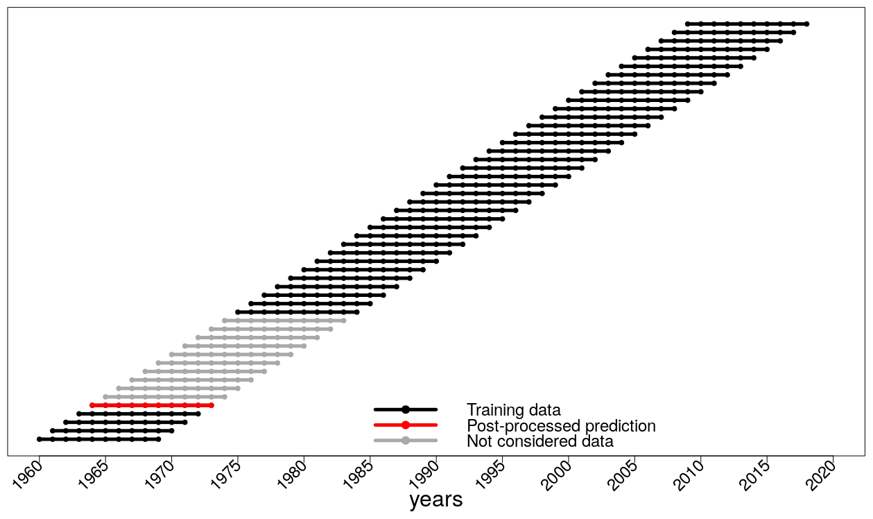
Figure 2Schematic overview of the cross-validation setting for a decadal climate prediction, initialized in 1964 (dotted red line). All hindcasts which are initialized outside the prediction period are used as training data (dotted black lines). A hindcast which is initialized inside the prediction period is not used for training (dotted gray lines).
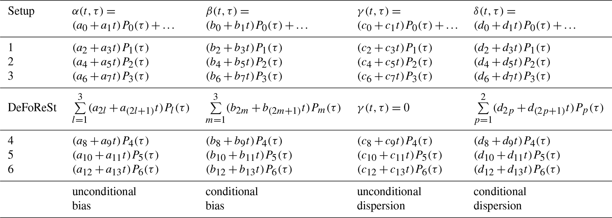
α(t,τ), β(t,τ), γ(t,τ) and δ(t,τ) are modeled using a similar approach as in Eqs. (10)–(12) where we now use orthogonalized polynomials to address for the lead time dependency of these corrections terms. In light of a model selection, this has the advantage that the individual predictors are uncorrelated. Moreover, for boosted recalibration, we use orthogonalized polynomials of sixth order in lead time τ, assuming that this is sufficiently large to capture all features of lead-time-dependent drift (α(t,τ)), conditional bias (β(t,τ)) and ensemble dispersion (γ(t,τ) and δ(t,τ)); the dependence on initialization time t is kept linear:
Here, and Pp(τ) are orthogonalized polynomials of order l, m, n and p, which are provided by the R function poly (R Core Team, 2018).
We apply boosting for non-homogeneous regression problems as proposed by Messner et al. (2017) for estimating al, bm, cn and dp. The algorithm iteratively seeks the minimum of a loss function (negative log likelihood or CRPS) by identifying and updating only the most relevant terms in the predictor.
This is realized with the R package
crch for non-homogeneous boosting (Messner et al., 2016, 2017) which uses a
minimization of the negative log likelihood by default instead of
minimizing the CRPS. Judging from our experience, for the problem at
hand, the difference in using one or the other loss function appears
to be small.
The above-mentioned effect of outliers and extremes on dispersivity described by Gneiting et al. (2005) should be rather small here, since annual aggregated values are recalibrated. Thus, we use the negative log likelihood as a cost function in the following.
In each iteration, the negative partial derivatives,
of the negative log-likelihood for a single observation y,
are obtained, where is the PDF of the normal distribution, μ the ensemble mean and σ the ensemble standard deviation corresponding to the initialization time t and lead time τ of the observation y. Pearson's correlation coefficient between each predictor term (e.g., t or t τ2) and the partial derivatives r and s (Eq. 20) estimated over every available and is used to identify and update the most influential term in the predictor. The parameter associated with the term with the highest correlation is updated by its correlation coefficient multiplied by a predefined step size ν. Schmid and Hothorn (2008) showed that the choice of ν is only of minor importance and suggested a value of 0.1. A smaller value for ν leads to an increase in precision in the updated coefficients at the expense of computing time. This allows a more detailed analysis of the relative importance of predictor variables. ν=0.05 turns out to be a reasonable compromise between precision and computing time in this setting. A distinct feature of boosting for non-homogeneous regression is that both mean and standard deviation of a forecast distribution are taken into account, but for each iteration step only one parameter (either associated with the mean μ𝙲𝚊𝚕,𝚋𝚘𝚘𝚜𝚝 or variance σ𝙲𝚊𝚕,𝚋𝚘𝚘𝚜𝚝) is updated: the one leading to the largest improvement of the cost function. Only those parameters associated with the most relevant predictor terms are updated; parameters of less relevant terms remain at zero. The algorithm is originally described in Messner et al. (2017); for reasons of convenience, we show in Fig. 3 a schematic flow chart of the boosting algorithm adopted to means of boosted recalibration.
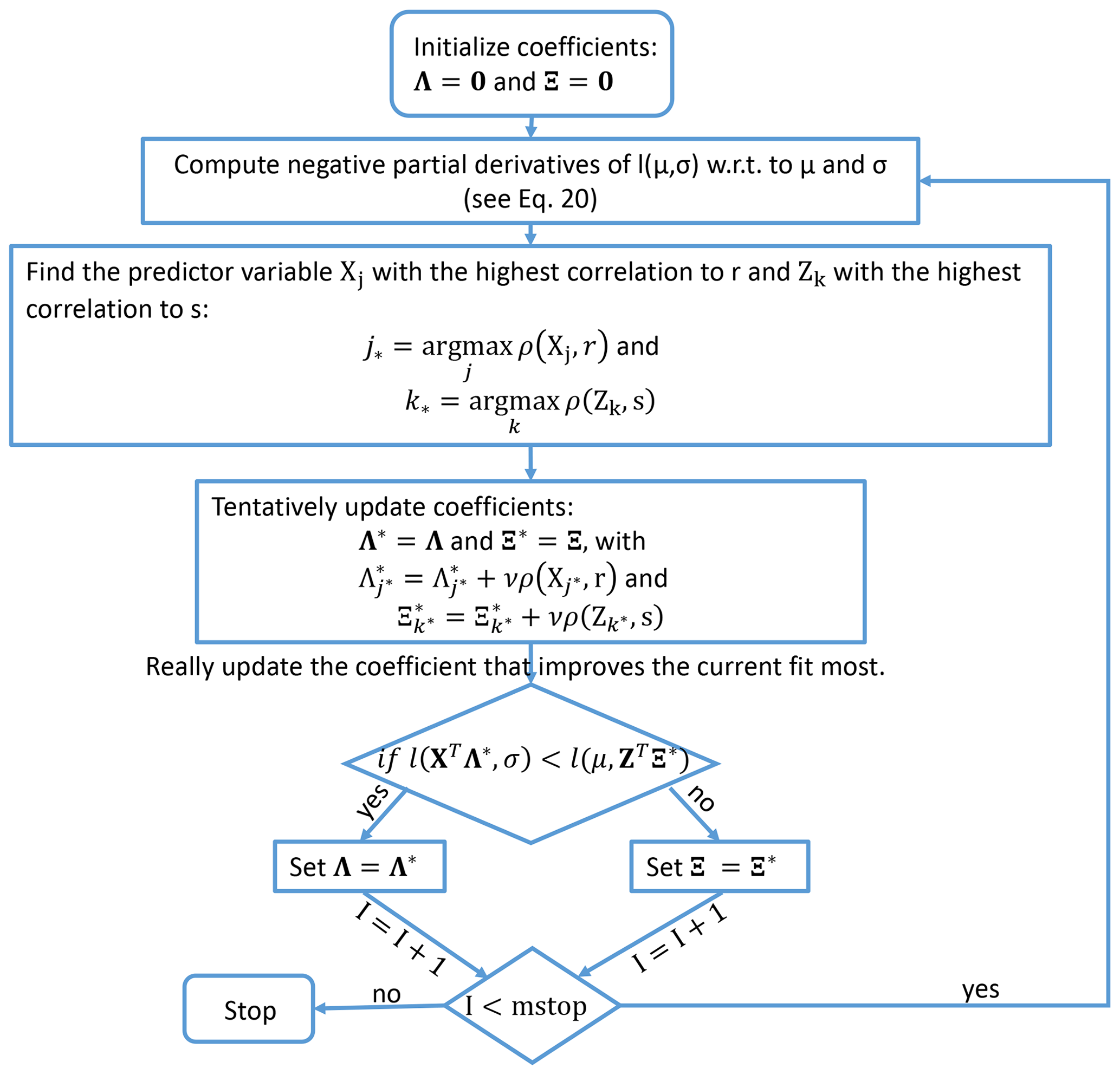
Figure 3Schematic flow chart for boosting algorithm proposed by Messner et al. (2016). For the ensemble mean and the ensemble variance, we use the expressions and , where and are vectors of predictor terms and and are vectors of the corresponding coefficients. Here, 0 is a vector of zeros, mstop is the predefined maximum number of boosting iteration steps I and ρ(Xj,r) as well as ρ(Zk,s) are the correlation coefficients calculated by Xj×r and Zk×s over the respective training data.
If the chosen iteration steps is small enough, a certain number of less relevant predictor terms have coefficients equal to zero, which prevents the model from overfitting. A cross-validation (CV) approach is used to identify the iteration with the set of parameter estimates with maximum predictive performance. Currently, CV is carried out after each boosting iteration. The data are split into five parts, and each part consists of approximately 10 years in order to reflect conditions of decadal prediction. For each part, a recalibrated prediction is computed, with the model trained on the remaining four parts. Afterwards, these five recalibrated parts are used to calculate the full negative log likelihood. Here, the full negative log likelihood results from summing Eq. (21) for all available t and τ and the associated observations y. The iteration step with minimum negative log likelihood is considered best. We allow a maximum number of 500 iterations.
Table 1Overview of the different toy model setups and the corresponding polynomial lead time dependencies.
Analog to the standard DeFoReSt, the previously described modeling procedure (boosting and CV for iteration selection) is carried out in a cross-validation setting (second level of CV) for model validation. A 10-year moving validation period (see Sect. 3.1) leads to cross-validation. For example, to recalibrate the hindcast initialized in 1963 including lead years 1964 to 1973, all hindcasts which are not initialized within that period (e.g., ) are used for boosting DeFoReSt.
To assess the model selection approach for DeFoReSt, we consider two toy model experiments with different potential predictabilities to generate pseudo-forecasts, as introduced by Pasternack et al. (2018). They are designed as follows:
-
the predictable signal is stronger than the unpredictable noise, and
-
the predictable signal is weaker than the unpredictable noise.
These experiments are controlled by five further parameters:
- η
-
determines the ratio between the variance of the predictable signal and the variance of the unpredictable noise, it controls potential predictability; see Pasternack et al. (2018). We investigate two cases: η=0.2 (low potential predictability) and η=0.8 (high potential predictability).
- χ(t,τ)
-
specifies the unconditional bias added to the predictable signal.
- ψ(t,τ)
-
analogously specifies the conditional bias.
- ω(t,τ)
-
specifies the conditional dispersion of the forecast ensemble.
- ζ(t,τ)
-
analogously controls the unconditional dispersion and has not been used in Pasternack et al. (2018).
The coefficients for bias (drift), conditional bias and effects in the ensemble dispersion are chosen such that they are close to those obtained from calibrating prototype surface temperature with HadCRUT4 observations. Thus, χ(t,τ), ψ(t,τ), ω(t,τ) and ζ(t,τ) are based on the same polynomial structure as used for the calibration parameters α(t,τ), β(t,τ), γ(t,τ) and δ(t,τ) (see Eqs. 16–19) (a detailed description of the toy model design is given in Appendix A). In the following, when we discuss the polynomial lead time dependency of the toy model's systematic errors, we refer to the polynomial order of α(t,τ), β(t,τ), γ(t,τ) and δ(t,τ). Note that the corresponding polynomials are also orthogonalized as in Eqs. (16)–(19).
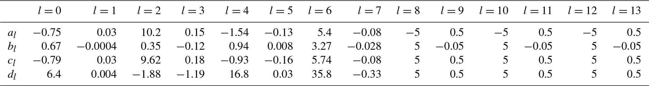
For an assessment of the model selection approach, we use seven different toy model setups per value of η. Each setup uses different orders of polynomial lead time dependency for imposing the above-mentioned systematic deviations on the predictable signal. One toy model setup is designed such that the corresponding systematic deviations could be perfectly addressed by DeFoReSt. Additionally, there are other setups with systematic deviations based on a lower/higher polynomial order than what is used for DeFoReSt. Thus, we compare pseudo-forecasts from setups which require model structures for recalibration given in Table 1.

Figure 4χ(t,τ) (a) and ψ(t,τ) (b) which are related to the unconditional and conditional bias, as well as ζ(t,τ) (c) and ω(t,τ) (d) which are related to the unconditional and conditional dispersion of the ensemble spread for the different toy model setups (colored lines) as a function of lead year τ with respect to start year t=1.
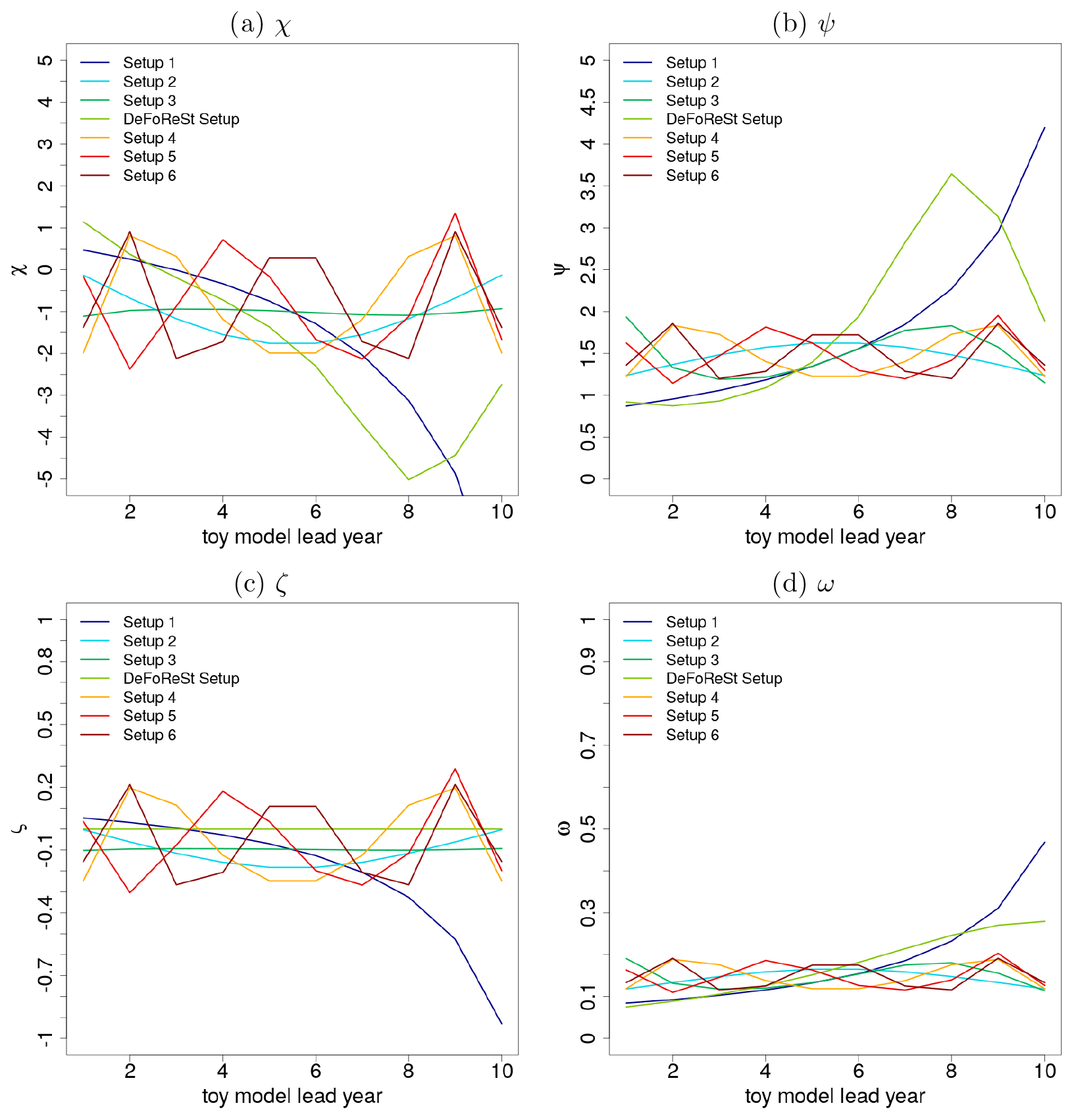
Figure 5χ(t,τ) (a) and ψ(t,τ) (b) which are related to the unconditional and conditional bias, as well as ζ(t,τ) (c) and ω(t,τ) (d) which are related to the unconditional and conditional dispersion of the ensemble spread for the different toy model setups (colored lines) as a function of lead year τ with respect to start year t=50.
As mentioned before, the functions χ(t,τ), ψ(t,τ), ζ(t,τ) and ω(t,τ) in the toy model experiments are based on the parameters estimated for calibrating the MiKlip prototype ensemble global mean surface temperature against HadCRUT4 observations. Here, χ(t,τ), ψ(t,τ), ζ(t,τ) and ω(t,τ) are based on ratios of polynomials up to third order with respect to lead time. Based on our experience, we assume that systematic errors with higher-than-third-order polynomials could not be detected sufficiently well within the MiKlip prototype experiments. Therefore, the coefficients for the fourth- to sixth-order polynomials are deduced from the coefficient magnitude of the first- to third-order polynomial. Here, it turns out that those coefficients associated with terms describing the lead time dependence exhibit roughly the same order of magnitude (see Fig. A1). Thus, we assume the coefficients associated with fourth- to sixth-order polynomials to be of the same order of magnitude. An overview of the applied coefficient values is given in Appendix A.
Analogously to the MiKlip experiment, the toy model uses 50 start years, each with 10 lead years, and 15 ensemble members. The corresponding pseudo-observations run over a period of 59 years in order to cover lead year 10 of start year 50. The corresponding imposed systematic errors for the unconditional and conditional bias (related to χ(t,τ) and ψ(t,τ)), unconditional and conditional dispersion (related to ζ(t,τ) and ω(t,τ)) are shown exemplarily for start year 1 and start year 50 in Figs. 4 and 5. Here, the effect of an increasing polynomial dependency in the lead time in setups 1 to 6 can be seen in the form of an increased variability. For the DeFoReSt setup, the systematic error manifests itself as a superposition of setups 1 to 3 for χ(t,τ) and ψ(t,τ) and of setups 1 to 2 for ω(t,τ) (ζ(t,τ) is equal to zero for the DeFoReSt setup). Regarding the influence of the start year, this effect amplifies for χ(t,τ) and ζ(t,τ) with increasing start time and diminishes for χ(t,τ) and ω(t,τ) due to their inverse definition (see Eqs. A10 and A12).
For each toy model setup, we calculated the ESS, the MSE, time mean intra-ensemble variance and the CRPSS of pseudo-forecasts recalibrated with boosting. References for the skill score are forecasts recalibrated with DeFoReSt. All scores have been calculated using cross-validation with an annually moving calibration window with a width of 10 years (see Pasternack et al., 2018).
To ensure a certain consistency, 1000 pseudo-forecasts are generated from the toy model and evaluated as described above. The scores presented are all mean values over these 1000 experiments. In particular, to assess a significant improvement of boosted recalibration over DeFoReSt with respect to CRPSS, the 2.5 % and 97.5 % percentiles are also estimated from these 1000 experiments.
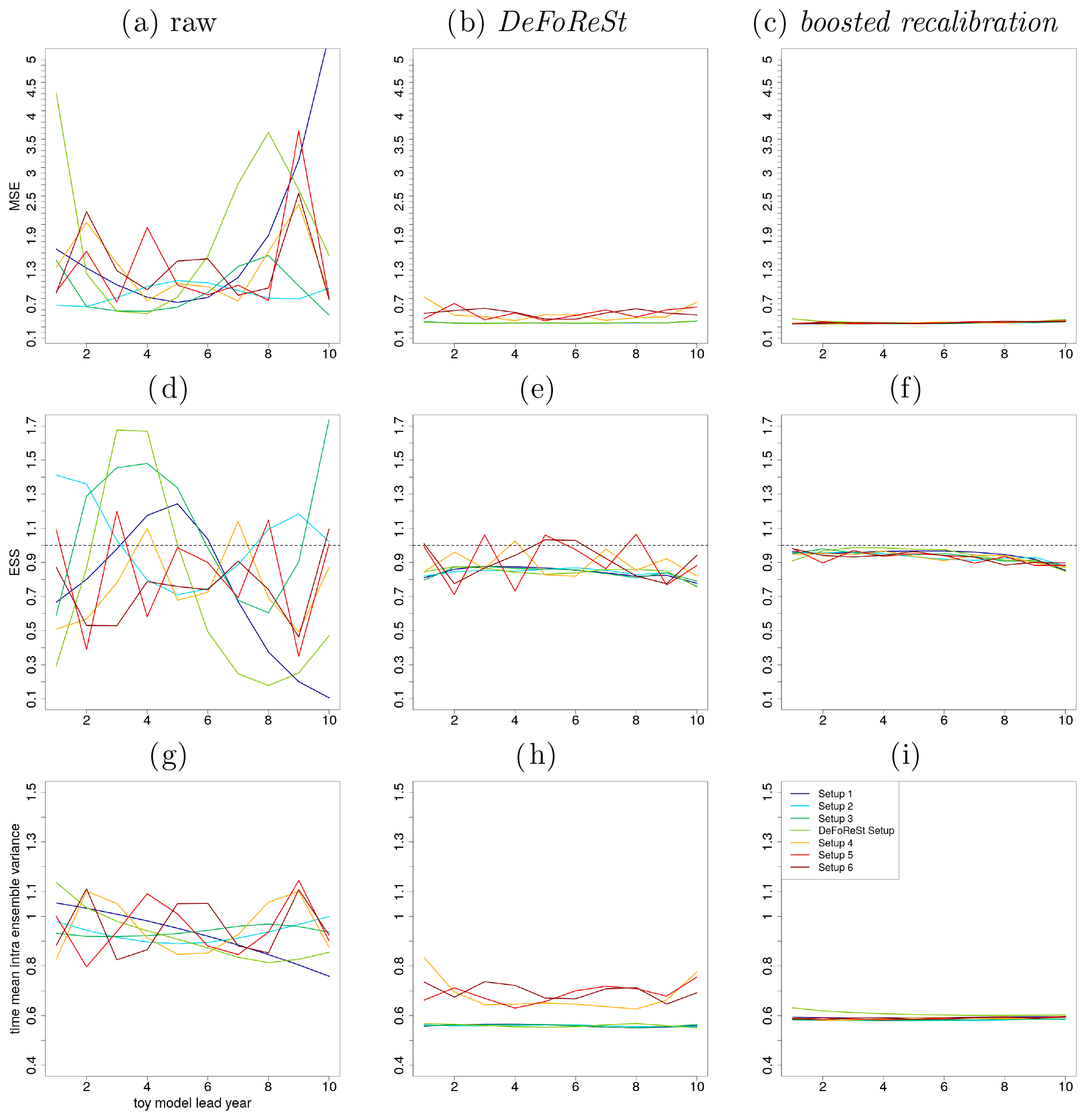
Figure 6Mean squared error (MSE) of different toy model setups with high potential predictability (η=0.8, colored lines). (a) Raw pseudo-forecast, (b) post-processing with DeFoReSt and (c) post-processing with boosted recalibration. Panels (d) to (f) show the ESS and (g) to (i) the intra-ensemble variance (temporal average), respectively.
4.1 Toy model setup with high potential predictability (η=0.8)
Figure 6a–c show the MSE for seven different setups (see Sect. 4). Panel (a) shows the result without any post-processing (raw pseudo-forecasts), panel (b) with DeFoReSt and panel (c) with boosted recalibration. Here, the performance of both post-processing methods is strongly superior to the raw pseudo-forecast output. As DeFoReSt uses third-order polynomials in lead time to capture conditional and unconditional biases, it performs equally as well as the boosted calibration for the first four setups; for setups using higher-order polynomials, boosted calibration is superior.
Regarding the ESS, Fig. 6d–f show that the raw pseudo-forecasts are widely fluctuating between under- and overdispersiveness (ESS values from 0.1 to 1.7), depending on the associated complexity of the imposed systematic errors (different setups). Corresponding to this, the post-processed pseudo-forecasts are more reliable with ESS values close to 1. The boosted recalibration approach is superior to the recalibration with DeFoReSt for every lead year. The improvement is largest for setups 4–6, because DeFoReSt is limited to third-order polynomials and cannot account for higher polynomial orders of these setups.
The post-processing methods are further compared by calculating the time mean intra-ensemble variance (see Fig. 6g–i). For every setup, the intra-ensemble variance of the raw pseudo-forecasts is higher than the intra-ensemble variance of corresponding post-processed forecasts. Comparing DeFoReSt with the boosted recalibration reveals that the sharpness of the first approach is larger for setups 1 to 3 and the “DeFoReSt setup”, leading particularly for the first three setups to an overconfidence (see Fig. 6e). However, for setups 4 to 6, DeFoReSt exhibits a smaller sharpness, which still results in combination with the increased MSE (see Fig. 6b) to underdispersiveness.
A joint measure for sharpness and reliability is the CRPS and its skill score, the CRPSS. Figure 7 shows the CRPSS of the different pseudo-forecasts with boosted recalibration, where pseudo-forecasts recalibrated with DeFoReSt are used as reference; i.e., positive values imply that boosted recalibration is superior to DeFoReSt. Colored dots in Fig. 7 denote significance in the sense that the 0.025 and 0.975 quantiles from the 1000 experiments do not include 0. Regarding setups 1 to 3 and the “DeFoReSt setup”, the CRPSS is neither significantly positive nor negative for all lead years. On the other hand, for setups 4 to 6 the boosted recalibration outperforms the recalibration with DeFoReSt with values of the CRPSS between 0.1 and 0.4. Again, this is likely due to DeFoReSt assuming third-order polynomials in lead time to capture conditional and unconditional biases and second order for dispersion, and therefore it does not account for systematic errors based on higher orders. However, Fig. 7 suggests that boosted recalibration can account for systematic errors with various levels of complexity.
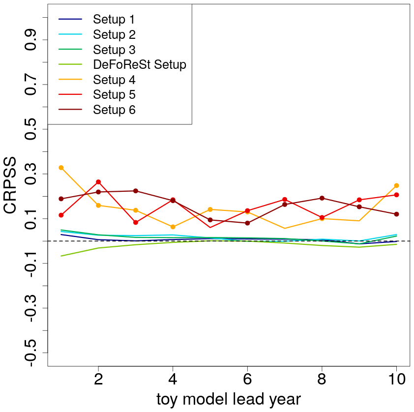
Figure 7CRPSS of different toy model setups with high potential predictability (η=0.8, colored lines) post-processed with boosted recalibration. The associated toy model setups post-processed with DeFoReSt are used as reference for the skill score. CRPSS larger zero implies boosted recalibration performing better than DeFoReSt. Colored dots in Fig. 7 denote significance in the sense that the 0.025 and 0.975 quantiles from the 100 experiments do not include 0.
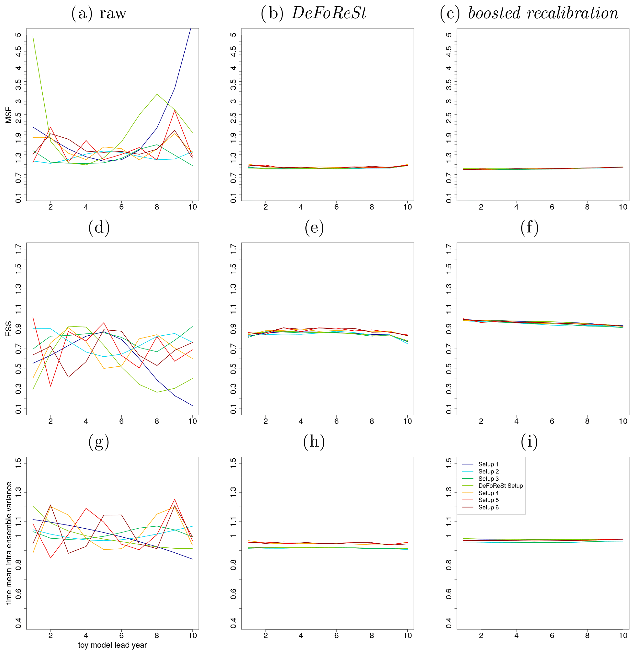
Figure 8MSE of different toy model setups with high potential predictability (η=0.2, colored lines). (a) Raw pseudo-forecast, (b) post-processing with DeFoReSt and (c) post-processing with boosted recalibration. Panels (d) to (f) show the ESS and (g) to (i) the intra-ensemble variance (temporal average), respectively.
4.2 Toy model setup with low potential predictability (η=0.2)
Figure 8a–c show the MSE of the different pseudo-forecasts for a toy model setup with a low potential predictability. One can see that both post-processing approaches lead to a strong improvement compared to the raw pseudo-forecasts; both approaches work roughly equally well for all setups. Compared to the previous section (η=0.8), the MSE of the pseudo-forecasts has increased due to a smaller signal-to-noise ratio.
The ESS (see Fig. 8d–f) reveals that compared to the pseudo-forecasts with high predictability, the raw simulations from different toy models are underdispersive for almost all lead years (ESS values smaller than 1). The pseudo-forecasts show again an increased reliability after recalibration, with ESS values close to 1. For every lead year, boosted recalibration is superior to DeFoReSt; the latter leads to slightly overconfident recalibrated forecasts.
Figure 8g–i show the time mean intra-ensemble variance of the raw and recalibrated pseudo-forecasts. For every setup, the intra-ensemble variance of the different pseudo-forecasts has decreased due to recalibration (with and without boosting). Comparing DeFoReSt with boosted recalibration reveals a smaller intra-ensemble variance for every setup, leading to an overconfidence for every lead year as observed in Fig. 8e.
In the low potential predictability setting (η=0.2), the ensemble variance is larger as the total variance in the toy model is constrained to one. Thus, reducing η leads to an increase in ensemble spread.
Figure 9 shows the CRPSS of the pseudo-forecasts with boosted recalibration with DeFoReSt as reference. The low potential predictability leads to a reduced CRPSS compared to the setting with η=0.8. The improvement due to boosted recalibration is also smaller. Only the first lead year of setups 4–6 is significantly different from zero. This suggests that the improvement due to boosted recalibration decreases with a decreasing potential predictability of the forecasts.
While in Sect. 4 DeFoReSt and boosted recalibration were compared by the use of different toy model data, in this section these two approaches will be applied to surface temperature of MiKlip prototype runs with MPI-ESM-LR. Here, global mean and spatial mean values over the North Atlantic subpolar gyre (50–65∘ N, 60–10∘ W) region will be analyzed.
We discuss which predictors are identified by boosted recalibration as most relevant and we compute the ESS, the MSE the intra-ensemble variance and the CRPSS with respect to climatology for both recalibration approaches. The scores have been calculated for a period from 1960 to 2010. In this section, a 95 % confidence interval was additionally calculated for these metrics using a bootstrapping approach with 1000 replicates. For bootstrapping, we randomly draw a new forecast–observation pair of dummy time series with replacement from the original validation period and calculate these scores again. This procedure has been repeated 1000 times. Please note that we draw for each model a new forecast–observation pair of dummy time series to avoid the metrics of these models being calculated on the basis of the same sample. Furthermore, all scores have been calculated using cross-validation with a yearly moving calibration window with a 10-year validation period (see Sect. 3.1).
5.1 Global mean surface temperature
Figure 10 shows the coefficients estimated by boosted recalibration for global mean surface temperature. The predictors are standardized; i.e., larger coefficients imply larger relevance of the corresponding predictors for the recalibration. Model selection is based on negative log-likelihood minimization in a cross-validation setup, as proposed by Pasternack et al. (2018). Thus, for every training period, different coefficients are obtained. The resulting distributions are represented in a box-and-whisker plot, which also allows an assessment of the variability in coefficient estimates.
Most relevant are the coefficients a0 and a1, associated with unconditional bias (a0), and the linear dependence on the start year (a1). This is followed by b0 in the conditional bias. In general, coefficients associated with first- and second-order terms in the lead time dependence (a2, a4, b2, b4) are dominating. Those coefficients describing the interaction between linear start year and first- or second-order lead year dependency (e.g., a3, b3, c3, b5, c5) have also been identified by the boosting algorithm as relevant.
The recalibration of ensemble dispersion is mostly influenced by a linear start year dependence in the unconditional term (c1) and in the conditional term d0. Higher terms are of minor relevance.
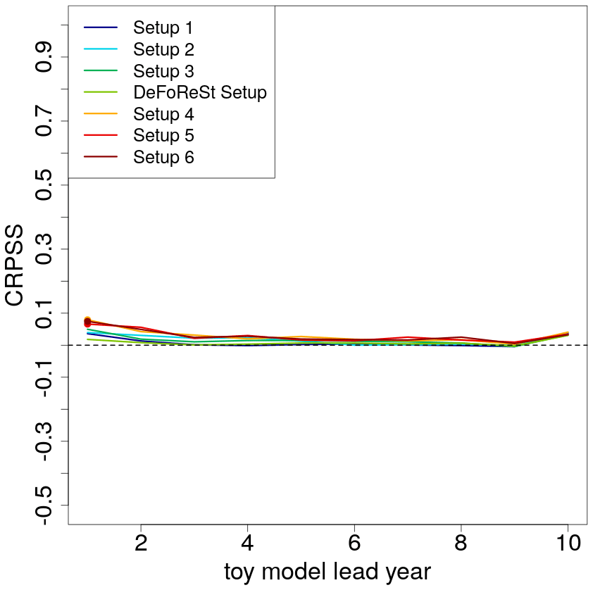
Figure 9CRPSS of different toy model setups with low potential predictability (η=0.2, colored lines) post-processed with boosted recalibration. The associated toy model setups post-processed with DeFoReSt are used as reference for the skill score. CRPSS larger zero implies boosted recalibration performing better than DeFoReSt. Colored dots indicate lead years with either significant positive or negative values based on a 95 % confidence interval from bootstrapping (100 repetitions).
The performance of the ensemble mean of the raw forecast (black), recalibrated with DeFoReSt (blue) and with boosted recalibration is measured with the MSE shown in Fig. 11a. While a strong drift (lead year dependence) influences the MSE for the raw forecasts, both recalibrated variants exhibit a smaller and roughly constant MSE across all τ. This decrease in MSE is a result of adjusting the unconditional and conditional bias (α(t,τ) and β(t,τ)).
Figure 11b evaluates the ensemble spread and shows the ESS. The raw pseudo-forecast is underdispersive (ESS < 1) for all lead years and needs recalibration. The recalibrated forecasts show an adequate ensemble spread in both cases (ESS close to 1) for all lead years. Boosted recalibration (red) outperforms DeFoReSt which becomes slightly under-/overdispersive for the first/last lead years. However, the differences in ESS between boosted recalibration and DeFoReSt are not significant.
Figure 11c shows the intra-ensemble variance (temporal average) across lead years τ. The ensemble variances of the raw forecast and DeFoReSt are roughly equal, while boosted recalibration adjusts the ensemble variance.
Compared to raw and DeFoReSt, the intra-ensemble variance of boosted recalibration is larger for lead year 1 and smaller for lead years 3 to 10. Boosted recalibration is sufficiently flexible to adjust the ensemble variance to a value close to the MSE. This consistent behavior is roughly constant over lead years.
Although boosted recalibration shows mostly a smaller ensemble variance (lead years 3–10) than DeFoReSt, both recalibration approaches are roughly equal when the performance is assessed with the CRPSS with climatological reference (Fig. 11d). Thus, the different time mean intra-ensemble variances resulting from recalibration with and without boosting have a minor impact on the CRPSS.
Here, the CRPSS of both models is around 0.8 for all lead years with respect to climatological forecast. In contrast, the raw forecast is inferior to the climatological forecast for most lead years, except lead years 3–6, where the raw forecast has positive skill, which could be attributed to the fact that temperature anomalies are considered. This implies that the observations and the raw forecast have the same mean value of 0. This mean value seems to be crossed by the raw forecast mainly between lead years 4 and 5.
5.2 North Atlantic mean surface temperature
Figure 12 shows the coefficients of the corresponding standardized predictors which were estimated using boosted recalibration for North Atlantic surface temperature. Analogously to the global mean surface temperature, model selection is used within a cross-validation setup and the resulting coefficient distributions are shown in a box-and-whisker plot. Here, the terms for the unconditional (ai) and conditional bias (bj) for the linear start year dependency (ait and bjt) and the first-order-polynomial lead time dependency (aiP1(τ) and bjP1(τ)) are most relevant. Moreover, the linear interaction between lead time and initialization time (a3 t P1(τ)) was identified as a relevant factor for the unconditional bias. Regarding the coefficients corresponding to the unconditional (ck) and conditional (dl) ensemble dispersion, one can see that the linear start and lead year dependencies (c1 t, c2 P1(τ) and d1 t, d2 P1(τ)), as well as the interaction (d3 t P1(τ)) between these two coefficients have the most impact.
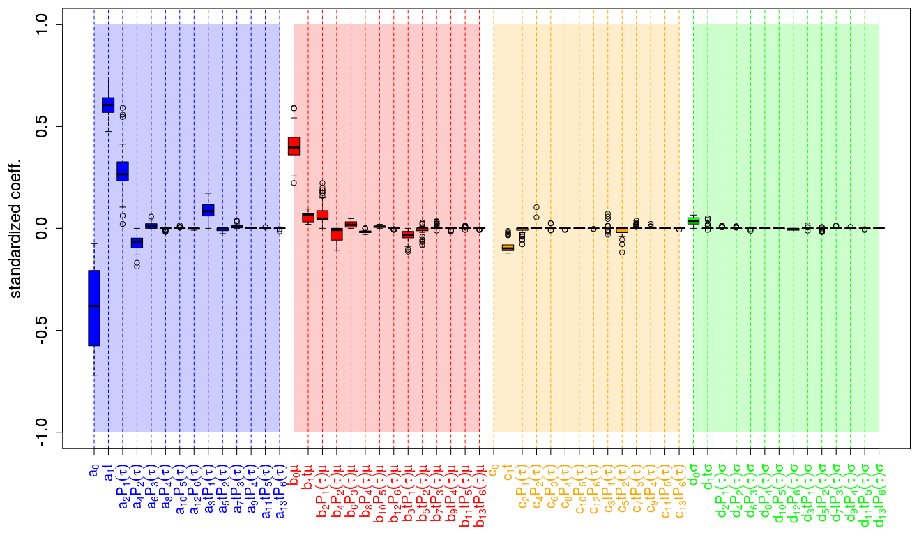
Figure 10Coefficient estimates for recalibrating global mean 2 m temperature of the MiKlip prototype system. Colored boxes represent the interquartile range (IQR) around the median (central, bold and black line) for coefficient estimates from the cross-validation setup; whiskers denote maximum 1.5 IQR. Coefficients are grouped according to correcting unconditional bias (blue), conditional bias (red), unconditional dispersion (orange) and conditional dispersion (green). Values refer to coefficients and not to the product between these coefficients and the corresponding predictors (e.g., a2 P1(τ) refers to a2). Please note that the value of c0 is around −2.5, but for a better overview the vertical axis is limited to the values range between −1 and 1. Vertical dashed bars highlight coefficients related to lead-time-dependent terms.
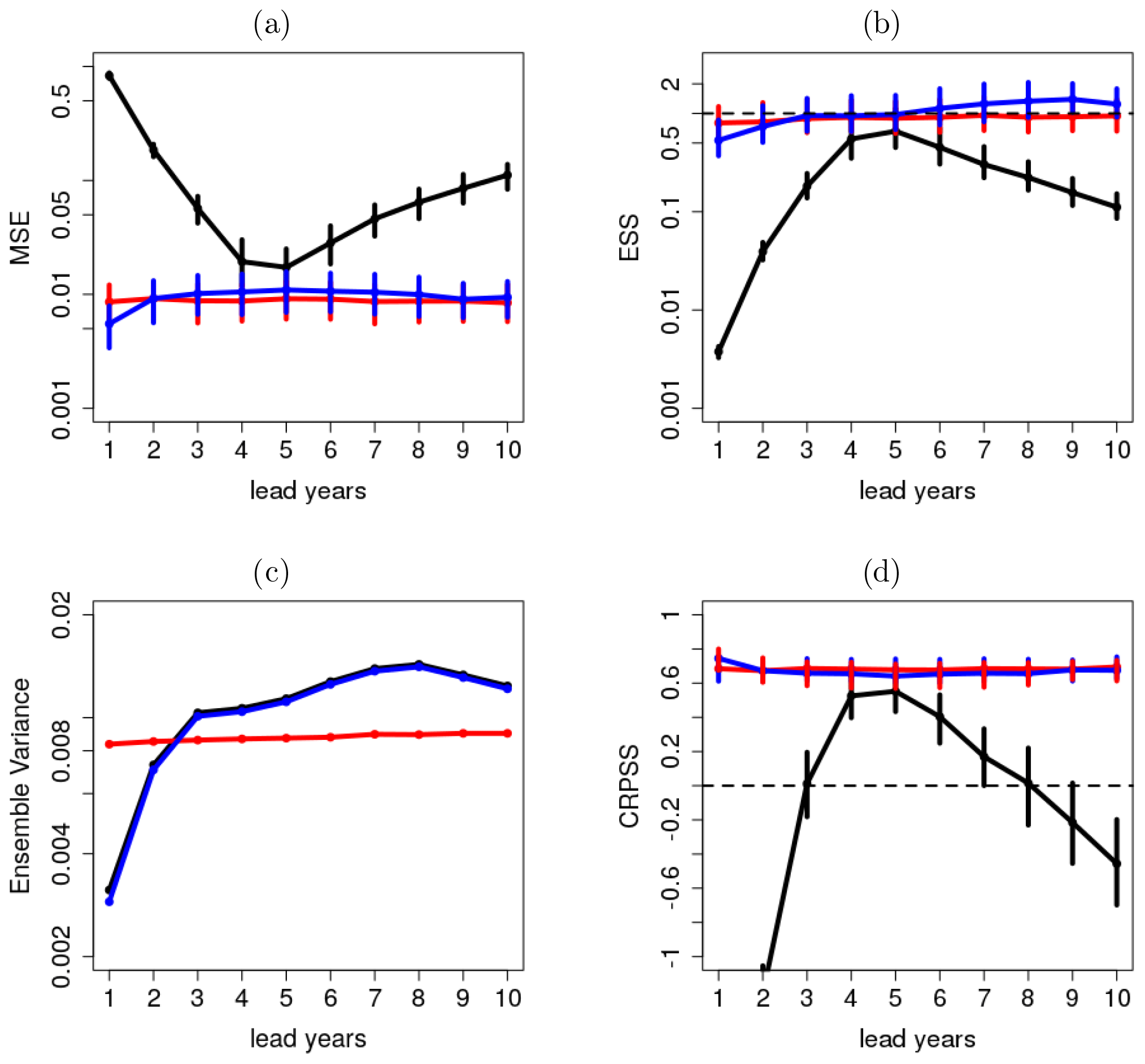
Figure 11(a) MSE, (b) reliability, (c) ensemble variance and (d) CRPSS of global mean surface temperature without any correction (black line), after recalibration with DeFoReSt (blue line) and boosted recalibration (red line). The CRPSS for the raw forecasts (black line) for lead year 1 is smaller than −1 and therefore not shown. The vertical bars show the 95 % confidence interval due to 1000-wise bootstrapping.
Figure 13a shows the MSE of the raw forecast (black), DeFoReSt and boosted recalibration, where both recalibrated forecasts perform roughly equally well. The raw forecast is inferior to both post-processed forecasts, mostly due to missing correction of unconditional and conditional biases. Compared to global mean temperature (Fig. 11a), MSE for the North Atlantic temperature is generally larger. Thus, potential predictability for the North Atlantic surface temperature is smaller than in the global case.
Regarding the reliability, both recalibrated forecasts also show an ESS close to 1 for all lead years for the North Atlantic surface temperature (Fig. 13b), which is similar to the outcome of the global mean temperature (Fig. 11b). Again boosted recalibration outperforms DeFoReSt, and the latter becomes slightly underdispersive for later lead years. However, the differences in ESS for both recalibration approaches are not significant. The raw forecast's reliability is obviously inferior here, as it is significantly underdispersive for lead years 1 to 3 and overdispersive for lead years 5 to 6.
The mentioned lower potential predictability for the North Atlantic manifests also in a 10 times larger ensemble variance; see Fig. 13c. It is noteworthy here that due to the smaller potential predictability in this region, the ensemble variance of both recalibrated forecasts is similar across the lead time and different from the raw forecast. A lower predictability of the North Atlantic surface temperature yields also a smaller CRPSS with respect to climatology for both recalibrated forecasts (Fig. 13d). Again, both recalibrated forecasts perform roughly equally well for all lead years and are also significantly to the raw forecast.
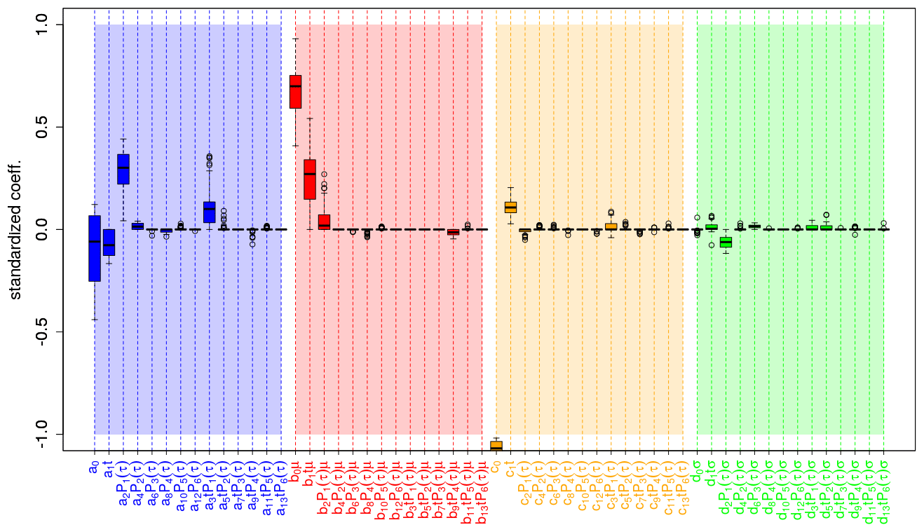
Figure 12Identified coefficients for recalibrating the mean 2 m temperature over the North Atlantic of the prototype. Here, the coefficients are grouped by correcting uncond. bias (blue bars), cond. bias (red bars), uncond. dispersion (orange bars) and cond. dispersion (green bars). The coefficients are standardized, i.e., with higher values implying a higher relevance. Values refer to coefficients and not to the product between these coefficients and the corresponding predictors (e.g., a2 P1(τ) refers to a2).
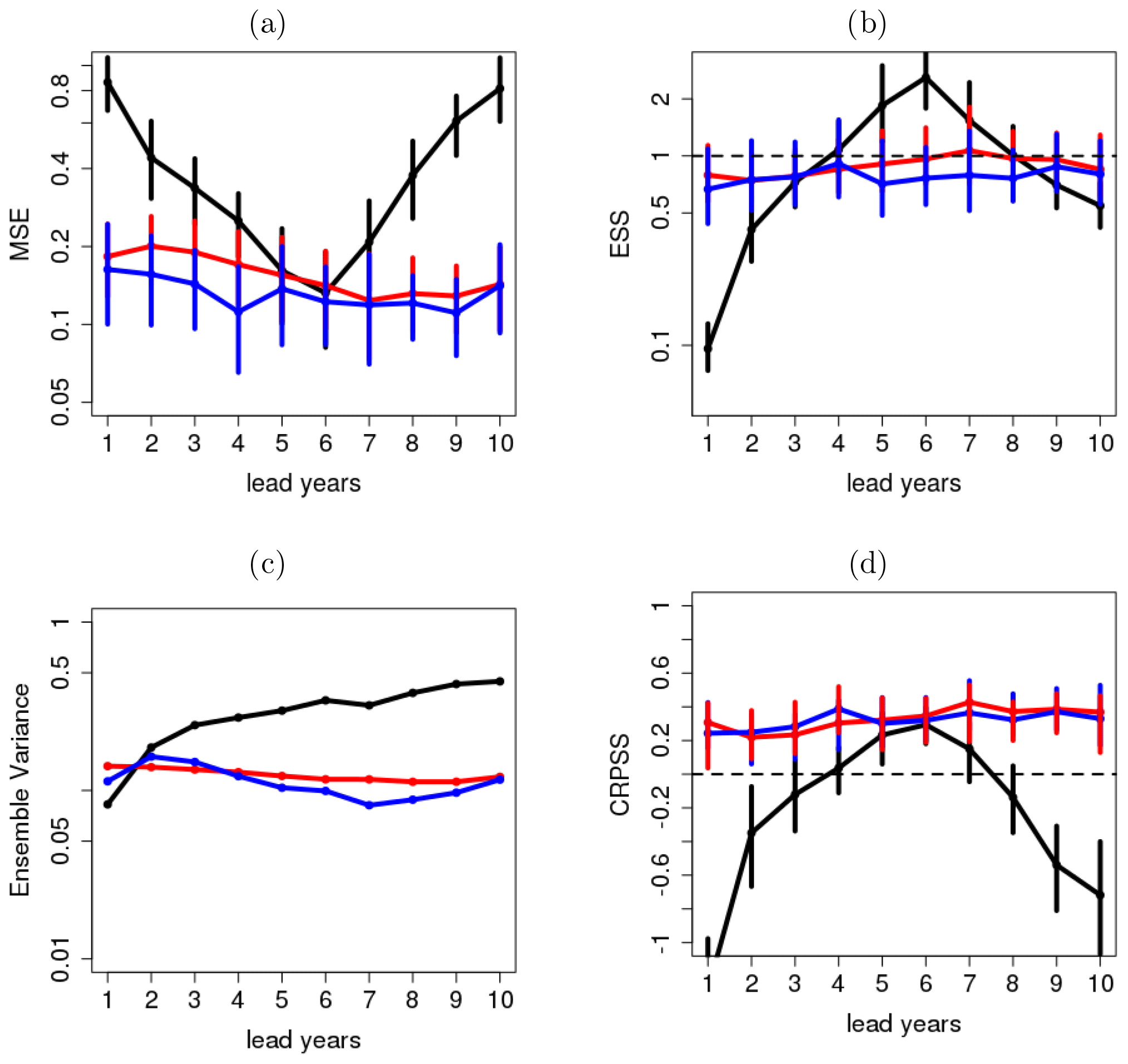
Figure 13(a) MSE, (b) reliability, (c) ensemble variance and (d) CRPSS of surface temperature over the North Atlantic without any correction (black line), after recalibration with DeFoReSt (blue line) and boosted recalibration (red line). The CRPSS for the raw forecasts (black line) for lead year 1 is smaller than −1 and therefore not shown. The vertical bars show the 95 % confidence interval due to 1000-wise bootstrapping.
Pasternack et al. (2018) proposed the recalibration strategy for decadal prediction (DeFoReSt) which adjusts non-homogeneous regression (Gneiting et al., 2005) to problems of decadal predictions. Characteristic problems here are a lead time and initialization time dependency of unconditional, conditional biases and ensemble dispersion. DeFoReSt assumes third-order polynomials in lead time to capture conditional and unconditional biases, second order for dispersion and first order for initialization time dependency. Although Pasternack et al. (2018) show that DeFoReSt leads to an improvement of ensemble mean and probabilistic decadal predictions, it is not clear whether these polynomials with predefined orders are optimal. This calls for a model selection approach to obtain a recalibration model as simple as possible and as complex as needed. We thus propose here not to restrict orders a priori to such a low order but use a systematic model selection strategy to determine optimal model orders. We use the non-homogeneous boosting strategy proposed by Messner et al. (2017) to identify the most relevant terms for recalibration. The recalibration approach with boosting (called boosted recalibration) starts with sixth-order polynomials in lead time and first order in initialization time to account for the unconditional and conditional bias, as well as for ensemble dispersion.
Common parameter estimation and model selection approaches such as stepwise regression and LASSO are designed for predictions of mean values. Non-homogeneous boosting jointly adjusts mean and variance and automatically selects the most relevant input terms for post-processing ensemble predictions with non-homogeneous (i.e., varying variance) regression. Boosting iteratively seeks the minimum of a cost function (here the log likelihood) and updates only the one coefficient with the largest improvement of the fit; if the iteration is stopped before a convergence criterion is fulfilled, the coefficients not considered until then are kept at zero. Thus, boosting is able to handle statistical models with a large number of variables.
We investigated boosted recalibration using toy model simulations with high (η=0.8) and low potential predictability (η=0.2) and errors with different complexities in terms of polynomial orders in lead time were imposed. Boosted recalibration is compared to DeFoReSt. The CRPSS, the ESS, the time mean intra-ensemble variance (a measure for sharpness) and the MSE assess the performance of the recalibration approaches. Scores are calculated with 10 year block-wise cross-validation (Pasternack et al., 2018) and with 100 pseudo-forecasts for each toy model simulation.
Irrespective of the complexity of systematic errors and the potential predictability, both recalibration approaches lead to an improved reliability with ESS close to 1. Sharpness and MSE can also be improved with both recalibration approaches. Given a high potential predictability (η=0.8), boosted recalibration – although allowing for much more complex adjustment terms – performs equal to DeFoReSt if systematic errors are less complex than a third-order polynomial in lead time, implied by the CRPSS of the pseudo-forecasts recalibrated with boosted recalibration and DeFoReSt as reference. Moreover, a significant improvement for almost all lead years can be observed if the complexity of systematic errors is larger than third-order polynomials in lead time. The gain with respect to DeFoReSt can hardly be observed for a low potential predictability (η=0.2), as the CRPSS shows only for two lead years a significant improvement for the above-mentioned complexities. This is due to a generally weaker predictable signal and thus a weaker impact of systematic error terms in the higher order of the polynomial. The improvement due to boosting increases with the imposed predictability. However, the presented toy model experiments suggest the use of boosted recalibration due to higher flexibility without loss of skill. Analogously to Pasternack et al. (2018), we recalibrated mean surface temperature of the MiKlip prototype decadal climate forecasts, spatially averaged over the North Atlantic subpolar gyre region and a global mean. Pronounced predictability for these cases has been identified by previous studies (e.g., Pohlmann et al., 2009; van Oldenborgh et al., 2010; Matei et al., 2012; Mueller et al., 2012). Nonetheless, both regions are also affected by a strong model drift (Kröger et al., 2018). For the global mean surface temperature, we could identify the linear start year dependency of the unconditional bias as a major factor. Moreover, it turns out that polynomials of lead year dependencies with order greater than 2 are of minor relevance.
Regarding the probabilistic forecast skill (CRPSS), DeFoReSt and boosted recalibration perform roughly equally well, implying that the polynomial structure of DeFoReSt, chosen originally from personal experience, turns out to be quite appropriate. Both recalibration approaches are reliable and outperforming the climatological forecast with a CRPSS near 0.8. This in line with the results from the toy model experiments which show that DeFoReSt and boosted recalibration perform similarly if systematic errors are less complex than a third-order polynomial in lead time. For the North Atlantic region, the linear start year and lead year dependencies of the unconditional and conditional biases show the largest relevance; also the linear interaction between lead time and initialization time of the unconditional bias has a certain impact. The coefficients corresponding to the unconditional and conditional ensemble dispersion show a minor relevance compared to the errors related to the ensemble mean.
Also for the North Atlantic surface temperature, both post-processing approaches are performing roughly equal; they are reliable and superior to climatology with respect to CRPSS. However, the CRPSS for the North Atlantic case is generally smaller than for the global mean.
This study shows that boosted recalibration, i.e., recalibration model selection with nonhomogeneous boosting, allows a parametric decadal recalibration strategy with an increased flexibility to account for lead-time-dependent systematic errors. However, while we increased the polynomial order to capture complex lead-time-dependent features, we still assumed a linear dependency in initialization time. As this model selection approach reduces parameters by eliminating irrelevant terms, this opens up the possibility to increase flexibility (polynomial orders) also in terms related to the start year.
Based on simulations from a toy model and the MiKlip decadal climate forecast system, we could demonstrate the benefit of model selection with boosting (boosted recalibration) for recalibrating decadal predictions, as it decreases the number of parameters to estimate without being inferior to the state-of-the-art recalibration approach (DeFoReSt).
The toy model proposed by Pasternack et al. (2018) consists of pseudo-observations x(t+τ) and associated ensemble predictions, hereafter named pseudo-forecasts f(t,τ).
Both are based on an arbitrary but predictable signal μx. Although it is almost identical to Pasternack et al. (2018), we quote the construction of pseudo-observations in the following for purposes of overview.
The pseudo-observation x is the sum of this predictable signal μx and an unpredictable noise term ϵx,
Following Kharin et al. (2012), μx can be interpreted as the atmospheric response to slowly varying and predictable boundary conditions, while ϵx represents the unpredictable chaotic components of the observed dynamical system. μx and ϵx are assumed to be stochastic Gaussian processes:
and
The variation of μx around a slowly varying climate signal can be interpreted as the predictable part of decadal variability; its amplitude is given by the variance . The total variance of the pseudo-observations is thus . Here, the relation of the latter two is uniquely controlled by the parameter , which can be interpreted as potential predictability ().
In this toy model setup, the concrete form of this variability is not considered and thus taken as random. A potential climate trend could be superimposed as a time-varying mean μ(t)=E[x(t)]. As for the recalibration strategy, only a difference in trends is important; we use μ(t)=0 and α(t,τ) addressing this difference in trends of forecast and observations.
The pseudo-forecast with ensemble members fi(t,τ) for observations x(t+τ) is specified as
where μens(t,τ) is the ensemble mean and
is the deviation of ensemble member i from the ensemble mean; is the ensemble variance. In general, ensemble mean and ensemble variance both can be dependent on lead time τ and initialization time t. We relate the ensemble mean μens(t,τ) to the predictable signal in the observations μx(t,τ) by assuming (a) a systematic deviation characterized by an unconditional bias χ(t,τ) (accounting also for a drift and difference in climate trends), a conditional bias ψ(t,τ) and (b) a random deviation ϵ(t,τ):
with being a random forecast error with variance . Although the variance of the random forecast error can in principle be dependent on lead time τ and initialization time t, we assume for simplicity a constant variance .
In contrast to the original toy model design, proposed by Pasternack et al. (2018), we assume an ensemble dispersion related to the variability of the unpredictable noise term ϵx with an unconditional and a conditional inflation factor (ζ(t,τ) and ω(t,τ)):
According to Eq. (A6) the forecast ensemble mean μens is simply a function of the predictable signal μx. In this toy model formulation, an explicit formulation of μx is not required; hence, a random signal might be used for simplicity, and it would be legitimate to assume without restricting generality. Here, we propose a linear trend in time to emphasize a typical problem encountered in decadal climate prediction: different trends in observations and predictions (Kruschke et al., 2015).
Given this setup, a choice of , , and would yield a perfectly calibrated ensemble forecast:
The ensemble mean μx(t,τ) of fperf(t,τ) is equal to the predictable signal of the pseudo-observations. The ensemble variance is equal to the variance of the unpredictable noise term representing the error between the ensemble mean of fperf(t,τ) and the pseudo-observations. Hence, fperf(t,τ) is perfectly reliable.
As mentioned in Sect. 4, this toy model setup is controlled on the one hand by η characterizing the potential predictability and on the other hand by χ(t,τ), ψ(t,τ), ζ(t,τ) and ω(t,τ), which control the unconditional and the conditional bias and the dispersion of the ensemble spread.
Here, χ(t,τ), ψ(t,τ), ζ(t,τ) and ω(t,τ) are obtained from α(t,τ), β(t,τ), γ(t,τ) and δ(t,τ) as follows:
The parameters χ(t,τ), ψ(t,τ), ζ(t,τ) and ω(t,τ) are defined such that a perfectly recalibrated toy model forecast fCal would have the following form:
Applying the definitions of μens (Eq. A6) and σens (Eq. A7) leads to
and applying the definitions of χ(t,τ), ψ(t,τ) and ω(t,τ) (Eqs. A9–A12) to Eq. (A14) would further lead to
This shows that fCal is equal to the perfect toy model fPerf(t,τ) (Eq. A8):
This setting has the advantage that the perfect estimation of α(t,τ), β(t,τ), γ(t,τ) and δ(t,τ) is already known prior to calibration with minimization of the logarithmic likelihood.
As described in Sect. 3.2, a sixth-order polynomial approach was chosen for unconditional α(t,τ), β(t,τ), γ(t,τ) and δ(t,τ), yielding
For the current toy model experiment, we exemplarily specify values for ai, bi, ci and di as obtained from calibrating the MiKlip prototype surface temperature over the North Atlantic against HadCRUT4 (Tobs):
where and specify the corresponding ensemble mean and ensemble spread. Here, χ(t,τ), ψ(t,τ), ζ(t,τ) and ω(t,τ) are based on ratios of polynomials up to third order with respect to lead time. Since systematic errors with higher-than-third-order polynomials could not be detected sufficiently well within the MiKlip prototype experiments, we deduce the coefficients for the fourth- to sixth-order polynomials from the coefficient magnitude of the first- to third-order polynomial. Here, Fig. A1 shows the coefficients which were obtained from calibrating the MiKlip prototype global mean surface temperature with cross-validation (see Pasternack et al., 2018), assuming a third-order polynomial dependency in lead years for α(t,τ), β(t,τ), γ(t,τ) and δ(t,τ). Those coefficients associated with terms describing the lead time dependence exhibit roughly the same order of magnitude. Thus, we assume the coefficients associated with fourth- to sixth-order polynomials to be of the same order of magnitude. The values of the coefficients are given in Table A1.
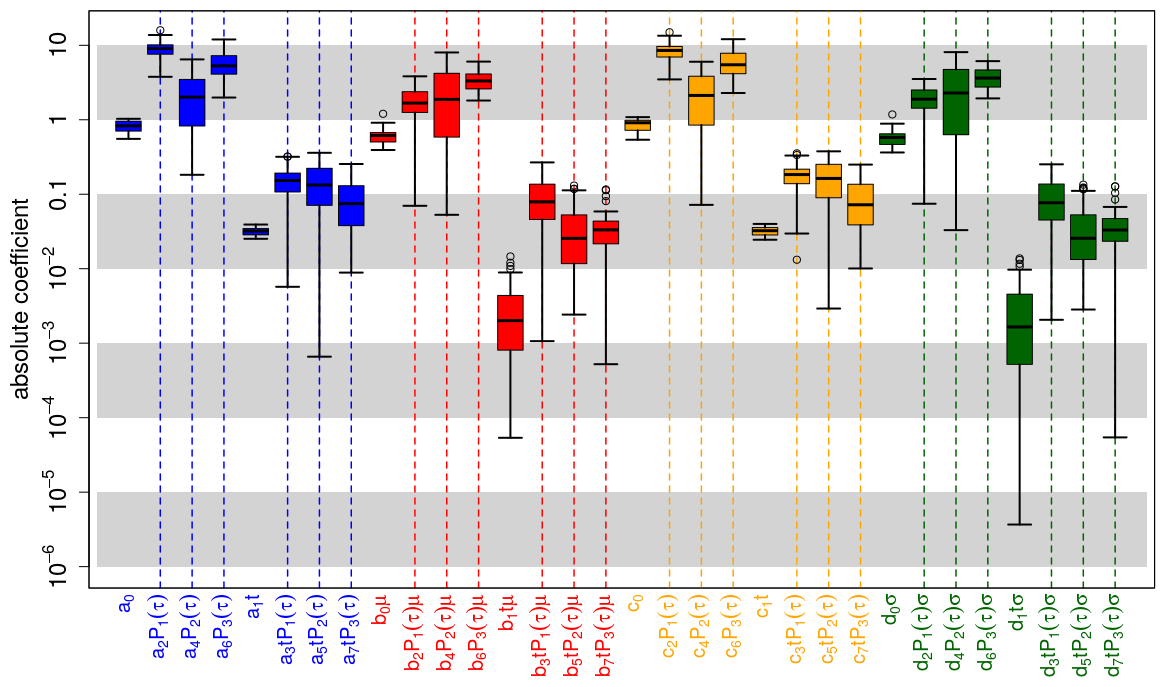
Figure A1Coefficient estimates for recalibrating global mean 2 m temperature of the MiKlip prototype system with a third-order polynomial lead time dependency for the unconditional and conditional bias and dispersion. Here, non-homogeneous boosting is not applied and all polynomials are orthogonalized; i.e., refer to the order of the corresponding polynomial. Colored boxes represent the IQR around the median (central, bold and black line) for coefficient estimates from the cross-validation setup; whiskers denote maximum 1.5 IQR. Coefficients are grouped according to correcting unconditional bias (blue), conditional bias (red), unconditional dispersion (orange) and conditional dispersion (green). Values refer to coefficients and not to the product between these coefficients and the corresponding predictors (e.g., a2 P1(τ) refers to a2). Vertical dashed bars highlight coefficients related to lead-time-dependent terms.
Table A1Overview of the values for the coefficients al, bl, cl and dl.
The HadCRUT4 global temperature dataset used in this study is freely accessible through the Climatic Research Unit at the University of East Anglia (https://crudata.uea.ac.uk/cru/data/temperature/HadCRUT.4.6.0.0.median.nc, Morice et al., 2012). The MiKlip prototype data used for this paper are from the BMBF-funded project MiKlip and are available on request. The post-processing, toy model and cross-validation algorithms are implemented using GNU-licensed free software from the R Project for Statistical Computing (http://www.r-project.org, last access: 7 July 2021) and can be found under https://doi.org/10.5281/zenodo.3975758 (Pasternack et al., 2020).
AP, JG, HWR and UU established the scientific scope of this study. AP, JG and HWR developed the algorithm of boosted recalibration and designed the toy model applied in this study. AP carried out the statistical analysis and evaluated the results. JG supported the analysis regarding post-processing of decadal climate predictions. HWR supported the statistical analysis. AP wrote the manuscript with contribution from all co-authors.
The authors declare that they have no conflict of interest.
Publisher’s note: Copernicus Publications remains neutral with regard to jurisdictional claims in published maps and institutional affiliations.
This research has been supported by the German Federal Ministry for Education and Research (BMBF) project
MiKlip (sub-projects CALIBRATION Förderkennzeichen FKZ 01LP1520A).
We acknowledge support from the Open Access Publication Initiative of Freie Universität Berlin.
This paper was edited by Ignacio Pisso and reviewed by three anonymous referees.
Anderson, J. L.: A method for producing and evaluating probabilistic forecasts from ensemble model integrations, J. Climate, 9, 1518–1530, 1996. a
Brohan, P., Kennedy, J. J., Harris, I., Tett, S. F., and Jones, P. D.: Uncertainty estimates in regional and global observed temperature changes: A new data set from 1850, J. Geophys. Res.-Atmos., 111, D12106, https://doi.org/10.1029/2005JD006548, 2006. a
Bühlmann, P. and Yu, B.: Boosting with the L 2 loss: regression and classification, J. Am. Stat. Assoc., 98, 324–339, 2003. a
Bühlmann, P. and Hothorn, T.: Boosting algorithms: Regularization, prediction and model fitting, Stat. Sci., 22, 477–505, 2007. a
Dee, D. P., Uppala, S. M., Simmons, A. J., Berrisford, P., Poli, P., Kobayashi, S., Andrae, U., Balmaseda, M. A., Balsamo, G., Bauer, P., Bechtold, P., Beljaars, A. C. M., van de Berg, I., Biblot, J., Bormann, N., Delsol, C., Dragani, R., Fuentes, M., Greer, A. J., Haimberger, L., Healy, S. B., Hersbach, H., Holm, E. V., Isaksen, L., Kallberg, P., Kohler, M., Matricardi, M., McNally, A. P., Mong-Sanz, B. M., Morcette, J.-J., Park, B.-K., Peubey, C., de Rosnay, P., Tavolato, C., Thepaut, J. N., and Vitart, F.: The ERA-Interim reanalysis: Configuration and performance of the data assimilation system, Q. J. Roy. Meteorol. Soc., 137, 553–597, https://doi.org/10.1002/qj.828, 2011. a
Feldmann, H., Pinto, J. G., Laube, N., Uhlig, M., Moemken, J., Pasternack, A., Früh, B., Pohlmann, H., and Kottmeier, C.: Skill and added value of the MiKlip regional decadal prediction system for temperature over Europe, Tellus A, 71, 1–19, 2019. a
Freund, Y. and Schapire, R. E.: A decision-theoretic generalization of on-line learning and an application to boosting, J. Comput. Syst. Sci., 55, 119–139, 1997. a
Friedman, J., Hastie, T., and Tibshirani, R.: Additive logistic regression: a statistical view of boosting (with discussion and a rejoinder by the authors), Ann. Stat., 28, 337–407, 2000. a
Fučkar, N. S., Volpi, D., Guemas, V., and Doblas-Reyes, F. J.: A posteriori adjustment of near-term climate predictions: Accounting for the drift dependence on the initial conditions, Geophys. Res. Lett., 41, 5200–5207, 2014. a
Gangstø, R., Weigel, A. P., Liniger, M. A., and Appenzeller, C.: Methodological aspects of the validation of decadal predictions, Climate Res., 55, 181–200, https://doi.org/10.3354/cr01135, 2013. a, b, c
Gneiting, T. and Katzfusss, M.: Probabilistic forecasting, Annual Review of Statistics and Its Application, 1, 125–151, 2014. a
Gneiting, T. and Raftery, A. E.: Strictly proper scoring rules, prediction, and estimation, J. Am. Stat. Assoc., 102, 359–378, 2007. a, b, c
Gneiting, T., Raftery, A. E., Westveld, A. H., and Goldman, T.: Calibrated probabilistic forecasting using ensemble model output statistics and minimum CRPS estimation, Mon. Weather Rev., 133, 1098–1118, 2005. a, b, c, d, e, f, g, h
Hamill, T. M. and Colucci, S. J.: Verification of Eta-RSM short-range ensemble forecasts, Mon. Weather Rev., 125, 1312–1327, 1997. a
Jolliffe, I. T. and Stephenson, D. B.: Forecast verification: a practitioner'sguide in atmospheric science, John Wiley & Sons, 2012. a
Jones, P. D., Lister, D. H., Osborn, T. J., Harpham, C., Salmon, M., and Morice, C. P.: Hemispheric and large-scale land-surface air temperature variations: An extensive revision and an update to 2010, J. Geophys. Res.-Atmos., 117, D05127, https://doi.org/10.1029/2011JD017139, 2012. a
Jungclaus, J. H., Fischer, N., Haak, H., Lohmann, K., Marotzke, J., Mikolajewicz, D. M. U., Notz, D., and von Storch, J. S.: Characteristics of the ocean simulations in the Max Planck Institute Ocean Model (MPIOM) the ocean component of the MPI-Earth system model, J. Adv. Model. Earth Syst, 5, 422–446, 2013. a
Keller, J. D. and Hense, A.: A new non-Gaussian evaluation method for ensemble forecasts based on analysis rank histograms, Meteorol. Z., 20, 107–117, 2011. a
Kharin, V. V., Boer, G. J., Merryfield, W. J., Scinocca, J. F., and Lee, W.-S.: Statistical adjustment of decadal predictions in a changing climate, Geophys. Res. Lett., 39, L19705, https://doi.org/10.1029/2012GL052647, 2012. a, b, c, d
Kruschke, T., Rust, H. W., Kadow, C., Müller, W. A., Pohlmann, H., Leckebusch, G. C., and Ulbrich, U.: Probabilistic evaluation of decadal prediction skill regarding Northern Hemisphere winter storms, Meteorol. Z., 25, 721–738, https://doi.org/10.1127/metz/2015/0641, 2015. a, b, c, d, e, f
Kröger, J., Pohlmann, H., Sienz, F., Marotzke, J., Baehr, J., Köhl, A., Modali, K., Polkova, I., Stammer, D., Vamborg, F., and Müller, W. A.: Full-field initialized decadal predictions with the MPI earth system model: An initial shock in the North Atlantic, Clim. Dynam., 51, 2593–2608, 2018. a, b
Köhl, A.: Evaluation of the GECCO2 ocean synthesis: transports of volume, heat and freshwater in the Atlantic, Q. J. Roy. Meteor. Soc., 141, 166–181, 2015. a
Maraun, D.: Bias correcting climate change simulations-a critical review, Curr. Clim. Change Rep., 2, 211–220, 2016. a
Marotzke, J., Müller, W. A., Vamborg, F. S. E., Becker, P., Cubasch, U., Feldmann, H., Kaspar, F., Kottmeier, C., Marini, C., Polkova,I., Prömmel, K., Rust, H. W., Stammer, D., Ulbrich, U., Kadow, C., Köhl, A., Kröger, J., Kruschke, T., Pinto, J., Pohlmann, H., Reyers, M., Schröder, M., Sienz, F., Timmreck, C., and Ziese, M.: Miklip – a national research project on decadal climate prediction, B. Am. Meteorol. Soc., 97, 2379–2394, 2016. a
Matei, D., Baehr, J., Jungclaus, J. H., Haak, H., Müller, W. A., and Marotzke, J.: Multiyear prediction of monthly mean Atlantic meridional overturning circulation at 26.5∘ N, Science, 335, 76–79, 2012. a, b
Meredith, E. P., Rust, H. W., and Ulbrich, U.: A classification algorithm for selective dynamical downscaling of precipitation extremes, Hydrol. Earth Syst. Sci., 22, 4183–4200, https://doi.org/10.5194/hess-22-4183-2018, 2018. a
Messner, J. W., Mayr, G. J., and Zeileis, A.: Heteroscedastic Censored and Truncated Regression with crch, R Journal, 8, 173–181, 2016. a, b
Messner, J. W., Mayr, G. J., and Zeileis, A.: Nonhomogeneous boosting for predictor selection in ensemble postprocessing, Mon. Weather Rev., 145, 137–147, 2017. a, b, c, d, e, f
Morice, C. P., Kennedy, J. J., Rayner, N. A., and Jones, P. D.: Quantifying uncertainties in global and regional temperature change using an ensemble of observational estimates: The HadCRUT4 data set, J. Geophys. Res.-Atmos., 117, D08101, https://doi.org/10.1029/2011JD017187, 2012. a, b
Mueller, W. A., Baehr, J., Haak, H., Jungclaus, J. H., Kröger, J., Matei, D., Notz, D., Pohlmann, H., Storch, J., and Marotzke, J.: Forecast skill of multi-year seasonal means in the decadal prediction system of the Max Planck Institute for Meteorology, Geophys. Res. Lett., 39, L22707, https://doi.org/10.1029/2012GL053326, 2012. a, b
Nelder, J. A. and Mead, R.: A simplex method for function minimization, Comput. J., 7, 308–313, 1965. a
Palmer, T., Buizza, R., Hagedorn, R., Lawrence, A., Leutbecher, M., and Smith, L.: Ensemble prediction: a pedagogical perspective, ECMWF newsletter, 106, 10–17, 2006. a, b, c, d
Pasternack, A., Bhend, J., Liniger, M. A., Rust, H. W., Müller, W. A., and Ulbrich, U.: Parametric decadal climate forecast recalibration (DeFoReSt 1.0), Geosci. Model Dev., 11, 351–368, https://doi.org/10.5194/gmd-11-351-2018, 2018. a, b, c, d, e, f, g, h, i, j, k, l, m, n, o, p, q, r, s, t, u, v, w, x, y, z, aa
Pasternack, A., Grieger, J., Rust, H. W., and Ulbrich, U.: Algorithms For Recalibrating Decadal Climate Predictions – What is an adequate model for the drift?, Zenodo, https://doi.org/10.5281/zenodo.3975759, 2020. a
Paxian, A., Ziese, M., Kreienkamp, F., Pankatz, K., Brand, S., Pasternack, A., Pohlmann, H., Modali, K., and Früh, B.: User-oriented global predictions of the GPCC drought index for the next decade, Meteorol. Z., 28, 3–21, 2018. a
Pohlmann, H., Jungclaus, J. H., Köhl, A., Stammer, D., and Marotzke, J.: Initializing decadal climate predictions with the GECCO oceanic synthesis: effects on the North Atlantic, J. Climate, 22, 3926–3938, 2009. a, b
Pohlmann, H., Mueller, W. A., Kulkarni, K., Kameswarrao, M., Matei, D., Vamborg, F., Kadow, C., Illing, S., and Marotzke, J.: Improved forecast skill in the tropics in the new MiKlip decadal climate predictions, Geophys. Res. Lett., 40, 5798–5802, 2013. a
R Core Team: R: A Language and Environment for Statistical Computing, R Foundation for Statistical Computing, Vienna, Austria, available at: https://www.R-project.org/ (last access: 7 July 2021), 2018. a, b
Sansom, P. G., Ferro, C. A. T., Stephenson, D. B., Goddard, L., and Mason, S. J.: Best Practices for Postprocessing Ensemble Climate Forecasts. Part I: Selecting Appropriate Recalibration Methods, J. Climate, 29, 7247–7264, https://doi.org/10.1175/JCLI-D-15-0868.1, 2016. a, b
Schmid, M. and Hothorn, T.: Boosting additive models using component-wise P-splines, Comput. Stat. Data Anal., 53, 298–311, 2008. a
Stevens, B., Giorgetta, M., Esch, M., Mauritsen, T., Crueger, T., Rast, S., Salzmann, M., Schmidt, H., Bader, J., Block, K., Brokopf, R., Fast, I., Kinne, S., Kornblueh, L., Lohmann, U., Pincus, R., Reichler, T., and Roeckner, E.: Atmospheric component of the MPI-M Earth System Model: ECHAM6, J. Adv. Model. Earth Syst., 5, 146–172, https://doi.org/10.1002/jame.20015, 2013. a
Talagrand, O., Vautard, R., and Strauss, B.: Evaluation of probabilistic prediction systems., Proc. Workshop on Predictability, Reading, United Kingdom, European Centre for Medium- Range Weather Forecasts, 25 pp., 1997. a
Uppala, S. M., Kållberg, P. W., Simmons, A. J., Andrae, U., Da Costa Bechtold, V., Fiorino, M., Gibson, J.K., Haseler, J., Her- nandez, A., Kelly, G. A., Li, X., Onogi, K., Saarinen, S., Sokka, N., Allan, R. P., Anderson, E., Arpe, K., Balmaseda, M. A., Beljaars, A. C. M., Van De Berg, L., Bidlot, J., Bormann, N., Caires, S., Chevallier, F., Dethof, A., Dragosavac, M., Fisher, M., Fuentes, M., Hagemann, S., Hólm, E., Hoskins, B. J., Isaksen, L., Janssen, P. A. E. M., Jenne, R., Mcnally, A. P., Mahfouf, J.-F., Morcrette, J.-J., Rayner, N. A., Saunders, R. W., Simon, P., Sterl, A., Trenbreth, K. E., Untch, A., Vasiljevic, D., Viterbo, P., and Woollen, J.: The ERA-40 re-analysis, Q. J. Roy. Meteor. Soc., 131, 2961–3012, https://doi.org/10.1256/qj.04.176, 2005. a
van Oldenborgh, G. J., Doblas Reyes, F., Wouters, B., and Hazeleger, W.: Skill in the trend and internal variability in a multi-model decadal prediction ensemble, in: EGU General Assembly Conference Abstracts, vol. 12, no. 9946, 2010. a, b
Weigend, A. S. and Shi, S.: Predicting daily probability distributions of S&P500 returns, J. Forecast., 19, 375–392, 2000. a
- Abstract
- Introduction
- Data and methods
- Model selection for DeFoReSt
- Calibrating toy model experiments
- Calibrating decadal climate surface temperature forecasts
- Conclusions
- Appendix A: Toy model construction
- Code and data availability
- Author contributions
- Competing interests
- Disclaimer
- Financial support
- Review statement
- References