the Creative Commons Attribution 4.0 License.
the Creative Commons Attribution 4.0 License.
 | 23 Mar 2021
A process-based evaluation of the Intermediate Complexity Atmospheric Research Model (ICAR) 1.0.1
Marlis Hofer
Ethan Gutmann
Alexander Gohm
Mathias W. Rotach
The evaluation of models in general is a nontrivial task and can, due to epistemological and practical reasons, never be considered complete. Due to this incompleteness, a model may yield correct results for the wrong reasons, i.e., via a different chain of processes than found in observations. While guidelines and strategies exist in the atmospheric sciences to maximize the chances that models are correct for the right reasons, these are mostly applicable to full physics models, such as numerical weather prediction models. The Intermediate Complexity Atmospheric Research (ICAR) model is an atmospheric model employing linear mountain wave theory to represent the wind field. In this wind field, atmospheric quantities such as temperature and moisture are advected and a microphysics scheme is applied to represent the formation of clouds and precipitation. This study conducts an in-depth process-based evaluation of ICAR, employing idealized simulations to increase the understanding of the model and develop recommendations to maximize the probability that its results are correct for the right reasons. To contrast the obtained results from the linear-theory-based ICAR model to a full physics model, idealized simulations with the Weather Research and Forecasting (WRF) model are conducted. The impact of the developed recommendations is then demonstrated with a case study for the South Island of New Zealand. The results of this investigation suggest three modifications to improve different aspects of ICAR simulations. The representation of the wind field within the domain improves when the dry and the moist Brunt–Väisälä frequencies are calculated in accordance with linear mountain wave theory from the unperturbed base state rather than from the time-dependent perturbed atmosphere. Imposing boundary conditions at the upper boundary that are different to the standard zero-gradient boundary condition is shown to reduce errors in the potential temperature and water vapor fields. Furthermore, the results show that there is a lowest possible model top elevation that should not be undercut to avoid influences of the model top on cloud and precipitation processes within the domain. The method to determine the lowest model top elevation is applied to both the idealized simulations and the real terrain case study. Notable differences between the ICAR and WRF simulations are observed across all investigated quantities such as the wind field, water vapor and hydrometeor distributions, and the distribution of precipitation. The case study indicates that the precipitation maximum calculated by the ICAR simulation employing the developed recommendations is spatially shifted upwind in comparison to an unmodified version of ICAR. The cause for the shift is found in influences of the model top on cloud formation and precipitation processes in the ICAR simulations. Furthermore, the results show that when model skill is evaluated from statistical metrics based on comparisons to surface observations only, such an analysis may not reflect the skill of the model in capturing atmospheric processes like gravity waves and cloud formation.
- Article
(6971 KB) - Full-text XML
- BibTeX
- EndNote


All numerical models of natural systems are approximations to reality. They generate predictions that may further the understanding of natural processes and allow the model to be tested against measurements. However, the complete verification or demonstration of the truth of such a model is impossible for epistemological and practical reasons (Popper, 1935; Oreskes et al., 1994). While the correct prediction of an observation increases trust in a model, it does not verify the model; e.g., correct predictions for one situation do not imply that the model works in other situations or even that the model arrived at the prediction through what would be considered the correct chain of events according to scientific consensus. In contrast, a model prediction that disagrees with a measurement falsifies the model, thereby indicating, for instance, issues with the underlying assumptions. From a practical point of view, the incompleteness and scarcity of data, as well as the imperfections of observing systems place further limits on the verifiability of models. The same limitations apply to model evaluation as well. However, evaluation focuses on establishing the reliability of a model rather than its truth.
These propositions include models employed in the Earth sciences, such as coupled atmosphere–ocean general circulation models, numerical weather prediction models and regional climate models. Those models approximate and simplify the world and processes in it by discretizing the governing equations in time and space and by modeling subgrid-scale processes with adequate parameterizations (e.g., Stensrud, 2009). The applied simplifications are often the result of a trade-off between physical fidelity of the modeled processes and the associated computational demand. However, even with a firm basis in natural laws, such models may generate results that match measured data but arrive at them through a causal chain differing from that inferred from observations (“right, but for the wrong reason”; e.g., Zhang et al., 2013). Additionally, the reason for a matching result may even be found in unphysical artifacts introduced by the numerical methods of these models (e.g., Goswami and O'Connor, 2010). In acknowledgment of the fundamental limitation of verification, models are evaluated rather than verified, and best practices and strategies have been outlined to maximize the probability that the results obtained from a model are correct for the right reasons (e.g., Schlünzen, 1997; Warner, 2011). Most of these criteria, however, apply to full physics-based models, such as regional climate models or numerical weather prediction models, that are expected to model atmospheric processes comprehensively.
The Intermediate Complexity Atmospheric Research model (ICAR; Gutmann et al., 2016) employed in this study is intended to be a simplified representation of atmospheric dynamics and physics over mountainous terrain. With a basis in linear mountain wave theory, it is a computationally efficient alternative to full physics regional climate models, such as the Weather Researching and Forecasting (WRF; Skamarock et al., 2019) model. Compared to simpler linear-theory-based models of orographic precipitation (e.g., Smith and Barstad, 2004), ICAR allows for a spatially and temporally variable background flow and a detailed vertical structure of the atmosphere and employs a complex microphysics scheme. However, for instance, precipitation induced by convection or enhanced by nonlinearities in the wind field is not considered by ICAR but may be accounted for with other methods (e.g., Jarosch et al., 2012; Horak et al., 2019). For such cases Schlünzen (1997) advises that a model has to be assessed with respect to its limit of application. Therefore, a direct comparison to a full physics-based model is generally not sufficient for an evaluation of ICAR since ICAR is not intended to provide a full representation of atmospheric physics. Furthermore, whether the results obtained from ICAR simulations are correct for the right reasons cannot be inferred from, for instance, precipitation measurements alone. Similar spatial distributions of precipitation may result from a variety of different atmospheric states. Therefore, the modeled processes yielding the investigated result need to be considered as well.
However, in the literature the evaluation efforts for ICAR have so far focused mainly on comparisons to precipitation measurements or WRF output. Gutmann et al. (2016) compared monthly precipitation fields for Colorado, USA, obtained from ICAR to WRF output and an observation-based gridded data set. While Gutmann et al. (2016) additionally performed idealized hill experiments, these focused on the qualitative comparison of the vertical wind field and the distribution of precipitation between ICAR and WRF. Bernhardt et al. (2018) applied ICAR to study changes in precipitation patterns in the European Alps that are dependent on the chosen microphysics scheme. Horak et al. (2019) evaluated ICAR for the South Island of New Zealand based on multi-year precipitation time series from weather station data and diagnosed the model performance with respect to season, atmospheric background state, synoptic weather patterns and the location of the model top. By comparing to measurements, Horak et al. (2019) observed a strong dependence of the performance of ICAR on the location of the model top, finding an optimal setting of 4.0 km above topography that minimized the mean squared errors calculated at all weather stations. However, the analysis of cross sections revealed numerical artifacts in the topmost vertical levels, suggesting these to be responsible for the high model skill, thus rendering the model right for the wrong reason.
This study aims to improve the understanding of the ICAR model and develop recommendations that maximize the probability that the results of ICAR simulations, such as the spatial distribution of precipitation, are correct and caused by the physical processes modeled by ICAR (correct for the right reasons) and not by numerical artifacts or any influence of the model top. For a given initial state, a correct representation of the fields of wind, temperature and moisture, as well as of the microphysical processes, are a necessity to obtain the correct distribution of precipitation. Therefore, simulations of an idealized mountain ridge are employed to investigate and evaluate the respective fields and processes in ICAR. This study first quantitatively and qualitatively analyzes how closely the ICAR wind and potential temperature fields match the analytical solution for the ideal ridge and contrasts them with a WRF simulation to infer the aspects not captured by linear theory (Sect. 4.1). In a second step the influence of the height of the model top and the upper boundary conditions on the microphysical cloud formation processes are quantified with a sensitivity study (Sects. 4.2–4.4). Thirdly, the differences in the hydrometeor and precipitation distribution due to nonlinearities and other processes not represented by linear theory are investigated in a comparison of ICAR to WRF (Sect. 4.5). Finally, the impact of recommendations derived from the preceding steps on a real case are demonstrated (Sect. 4.6). The case study is conducted for the South Island of New Zealand and contrasted to the results of Horak et al. (2019). All findings are discussed in Sect. 5, and the conclusions, including the recommendations, are summarized in Sect. 6.
2.1 Model description
ICAR is an atmospheric model based on linear mountain wave theory (Gutmann et al., 2016). The input data sets required by ICAR are a digital elevation model supplying the high-resolution topography h(x,y) and forcing data, i.e., a set of 4-D atmospheric variables as supplied by atmospheric reanalysis such as ERA5 or coupled atmosphere–ocean general circulation models. The forcing data set represents the background state of the atmosphere and must comprise the horizontal wind components (U,V), pressure p, potential temperature Θ and water vapor mixing ratio qv0.
ICAR stores all dependent variables on a 3-D staggered Arakawa C-grid (Arakawa and Lamb, 1977, pp. 180–181) and employs a terrain-following coordinate system with constant grid cell height. In particular, mass-based quantities such as water vapor are stored at the grid cell center, while the horizontal wind components u and v are stored at the centers of the west–east or south–north faces of the grid cells, and the vertical wind component w is stored at the center of the top–bottom faces of each grid cell.
In contrast to dynamical downscaling models, ICAR avoids solving the Navier–Stokes equations of motion explicitly. Instead, ICAR calculates the perturbations to the horizontal background winds analytically for a given time step by employing linearized Boussinesq-approximated governing equations that are solved in frequency space with the Fourier transformation (Barstad and Grønås, 2006). With the Fourier transform of, for example, the east–west wind perturbation u′ denoted as the perturbations to the horizontal wind field are
with the horizontal wavenumbers k and l, the Coriolis term f, and the imaginary number i. The vertical wavenumber m, the intrinsic frequency σ, and the fluid displacement are given by
Here denotes the Fourier transform of the topography h(x,y), z the elevation and N the Brunt–Väisälä frequency. Note that depending on whether a grid cell is saturated or not, either the moist, Nm (Emanuel, 1994), or dry, Nd, Brunt–Väisälä frequency is employed in Eq. (4) and calculated as
with the acceleration due to gravity g, the temperature T, the potential temperature θ, the equivalent potential temperature θe, the saturated adiabatic lapse rate Γm, the saturation mixing ratio qs, the cloud water mixing ratio qc, and the total water content and the specific heats at constant pressure of dry air and liquid water cp and cl. Note that ICAR employs quantities from the perturbed state of the domain to calculate N even though in linear mountain wave theory N is a property of the background state (e.g., Durran, 2015). Statically unstable atmospheric conditions (i.e., N2<0) in the forcing data are avoided by enforcing a minimum Brunt–Väisälä frequency of throughout the domain.
The vertical wind speed perturbation is calculated from the divergence of the horizontal winds u and v, where and , as follows:
ICAR does solve the Eqs. (1)–(8) for every grid cell in the ICAR domain separately and for every forcing time step as to allow for a spatially and temporally variable background state. To make this task computationally viable, ICAR employs a lookup table; see Gutmann et al. (2016) for details.
ICAR allows for the selection of different microphysics (MP) schemes. In this study an updated version of the Thompson MP scheme is employed (Thompson et al., 2008). It predicts mixing ratios for water vapor qv, cloud water qc, cloud ice qi, rain qr, snow qs and graupel qg, from here on referred to as microphysics species, as well as the number concentrations for cloud ice ni and rain nr. The Thompson MP scheme is a double-moment scheme in cloud ice and rain and a single-moment scheme for the remaining quantities.
The microphysics species, ni, nr and θ are advected with the calculated wind field according to the advection equation (Gutmann et al., 2016):
where ψ denotes any of the advected quantities. At the lateral domain boundaries L located at nx=0, nx=Nx, ny=0, and ny=Ny, where Nx and Ny are the number of grid points along the x and y direction, the value of ψ is given by the forcing data set and specified by a Dirichlet boundary condition as
with ψF as the respective quantity in the forcing data set temporally and spatially interpolated to the ICAR grid and model time. At the upper boundary T where nz=Nz and Nz as the grid points along the z direction, a zero-gradient Neumann boundary condition is imposed:
The initial conditions at t0 for the 3-D fields of all atmospheric quantities Ψ in the ICAR domain are prescribed by linearly interpolating the corresponding field in the forcing data set ΨF to the high-resolution ICAR domain:
Note that capital Ψ denotes not only the advected quantities ψ but also p.
In linear mountain wave theory, the wind field is entirely determined by the topography and the background state of the atmosphere (Sawyer, 1962; Smith, 1979) and, for a horizontally and vertically homogeneous background state, given by a set of analytical equations (e.g., Barstad and Grønås, 2006). This formal simplicity is achieved by a number of simplifications, for instance neglecting the interaction of waves with waves; waves with turbulence or nonlinear effects such as gravity wave breaking, time-varying wave amplitudes, or low-level blocking and flow splitting. Discussions of the limitations of linear theory resulting from this reduction of complexity can be found in the literature (e.g., Dörnbrack and Nappo, 1997; Nappo, 2012).
Note that since ICAR is based on the equations derived by Barstad and Grønås (2006), it currently neglects the reflection of waves at the interface of atmospheric layers with different Brunt–Väisälä frequencies. Furthermore, it neglects the vertical increase of the amplitude of the wind field perturbations with decreasing density. A full description of ICAR is given by Gutmann et al. (2016).
2.2 Modifications to ICAR
The investigations described in this study were conducted with a modified version of ICAR 1.0.1. All modifications are publicly available for download (Gutmann et al., 2020).
2.2.1 Calculation of the Brunt–Väisälä frequency
From the initial state of θ and the microphysics species fields at t0 (see Eq. 12), ICAR calculates the (moist or dry; see Eqs. 6 and 7, respectively) Brunt–Väisälä frequency N for all model times tm smaller than the first forcing time . During each model time step, the θ and microphysics species fields in the ICAR domain are modified by advection and microphysical processes. Therefore, for model times tm>t0, θ and all the microphysics species, q represents the perturbed state of the respective fields, denoted as
Note that in this notation, the perturbed water vapor field is denoted as qv, the background state water vapor field as qv0 and the perturbation field as . Consequently, during all intervals , where are subsequent forcing time steps, N is based on the perturbed states of potential temperature and the microphysics species at . More specifically, all atmospheric variables ICAR uses for the calculation of N with Eqs. (6) and (7) are represented by the perturbed fields.
However, in linear mountain wave theory N is a property of the unperturbed background state (e.g., Durran, 2015), an assumption that is not satisfied by the calculation method employed by the standard version of ICAR. This study therefore employs a modified version of ICAR that, in accordance with linear mountain wave theory, calculates N from the state of the atmosphere given by the forcing data set if the corresponding option is activated. In the following, the modification of ICAR basing the calculation of N on the background state is referred to as ICAR-N, while the unmodified version, which bases the calculation on the perturbed state of the atmosphere, is referred to as the original version (ICAR-O). If properties applying to both versions are discussed, the term ICAR is chosen.
2.2.2 Treatment of the upper boundary in the advection numerics
ICAR imposes a zero-gradient boundary condition (ZG BC) at the upper boundary on all quantities subject to numerical advection; see Eq. (11). This section details how, specifically for the microphysics species, a ZG BC has the potential to cause problems by, e.g., triggering influx of additional water vapor into the domain. Due to its conceptual simplicity, the issue is illustrated for the upwind advection scheme, which is the standard advection scheme employed by ICAR.
In the following, the mass levels are indexed from 1 to Nz and the half levels bounding the kth mass level are denoted as and . Note that the vertical wind components are calculated at half levels with Eq. (8) and that, in particular, no boundary condition is required to determine w at the model top.
To arrive at the discrete equations of the upwind advection, the flux divergences , and on the right-hand side of Eq. (9) are discretized as, e.g., in Patankar (1980). The vertical flux gradient ϕz across mass level k at time step t due to downdrafts ( and ) is then approximated by
with Δz as the vertical grid spacing. The resulting value of ψ at mass level k at time step t+1 is calculated with an explicit first-order Euler forward scheme as
where Δt denotes the length of the time step. At the upper boundary, where k=Nz, with Nz being the number of vertical levels, by default ICAR applies a zero-gradient boundary condition to ψ by setting . In case of downdrafts, and vertical convergence in the wind field across the topmost vertical mass level (), this results in a negative vertical flux gradient and an associated increase in ψ (see Eq. 16). If persists for more than one time step, the concentration of the quantity in the topmost vertical level will continue to increase until it is redistributed within the domain via advection or conversion into other microphysics species. As observed by Horak et al. (2019), this influx of additional water therefore may cause numerical artifacts such as the formation of spurious clouds.
While the effect described above is related to downdrafts at the model top, note that updrafts, on the other hand, may cause moisture to be transported out of the domain, leading to a mass loss. However, for k=Nz and and , the discretization of the vertical flux divergence in Eq. (9) yields
Therefore, this issue cannot be addressed by applying different boundary conditions, since Eq. (17) does not depend on .
A solution to address both issues would potentially be to include a relaxation layer directly beneath the model top (see, e.g., Skamarock et al., 2019). Within this relaxation layer, vertical wind speeds would tend towards zero with decreasing distance to the model top and perturbed quantities would be relaxed towards their value in the background state. Another potential solution is employed by full physics models such as the Integrated Forecasting System (IFS) of the European Center for Medium-Range Weather Forecasts (ECMWF, 2018), the COSMO model (Doms and Baldauf, 2018) or the Weather Research and Forecasting (WRF) model (Skamarock et al., 2019). These models place the location of the upper boundary at elevations high enough that moisture fluxes across the boundary are negligible. While applying either treatment to ICAR is, in general, an option, it is undesirable since both necessarily result in higher model tops and therefore would severely increase the computational cost of ICAR simulations. Hence, this study investigates whether the application of computationally cheaper alternative boundary conditions is able to reduce errors caused by, e.g., the unphysical mass influx and loss described above. To this end, additional boundary conditions are added to the ICAR code with the option to apply different boundary conditions to different quantities ψ. Furthermore, this study assesses whether the lowest possible model top elevation necessary to avoid the model top's impact on the results can be chosen substantially below that of full physics models without sacrificing the physical fidelity of the results.
To investigate ICAR with respect to the influence of the elevation of the upper boundary and the boundary conditions applied to it, idealized numerical simulations and a real case study are conducted. Simulations are run with ICAR-O, ICAR-N and WRF in order to assess to what degree ICAR simulations approximate the results of the analytical solution and a full physics model. In addition, WRF is employed to infer differences due to nonlinearities.
3.1 Simulation setup
Simulations in this study are conducted with version 1.0.1 of ICAR (ICAR-O) and version 4.1.1 of WRF. Additionally, a modification of ICAR-O, referred to as ICAR-N, where the Brunt–Väisälä frequency N is calculated from the background state given by the forcing data set is employed. Note that ICAR-O, on the other hand, calculates N from the perturbed state of the atmosphere predicted by the ICAR-O. In the idealized simulations the forcing data set is represented by an idealized sounding while for the real case it is the ERA-Interim reanalysis. For idealized simulations, a period of 18 h is used for spinup and the model output from t=19 h to t=30 h, with an interval of 1 h, is evaluated. The ICAR setup for the real case is described in Horak et al. (2019).
The ideal case consists of an infinite ridge extending along the south–north direction in the domain and westerly flow. The horizontal grid spacings of ICAR and WRF are chosen as with 404 grid points along the west–east axis and open boundary conditions at the western and eastern boundaries. Since ICAR does not currently support periodic boundary conditions, 104 grid points are employed along the south–north axis to minimize the influence of the boundaries on the domain center. For ICAR, open boundary conditions are imposed at the southern and northern boundaries. WRF, on the other hand, just uses three grid points along the south–north axis and periodic boundary conditions. The vertical spacing in ICAR simulations is set to Δz=200 m, while the 26 km high WRF domain is subdivided in 130 grid cells, resulting in an average vertical spacing of approximately 200 m. At the lower boundary ICAR and WRF employ a free-slip boundary condition. An implicit Rayleigh dampening layer (Klemp et al., 2008) is applied to the uppermost 16 km of the WRF domain, with a dampening coefficient of 0.3 s−1. The model time step of ICAR is automatically calculated by ICAR to satisfy the Courant–Friedrichs–Lewy criterion (Courant et al., 1928; Gutmann et al., 2016) and is approximately 40 s, while for WRF it is set to 2 s.
Idealized ICAR simulations are run for different model top elevations. The elevation of the upper boundary of the domain, referred to as model top elevation ztop, is increased by adding additional vertical levels while keeping the vertical spacing constant. The lowest model top is set at 4.4 km while the highest is located at 14.4 km, with steps of 1 km in between. The lower end of the model top range reflects the lowest settings employed in preceding studies, such as Horak et al. (2019), where the optimal setting was determined at 4.0 km, or Gutmann et al. (2016), who set the top of the ICAR domain to 5.64 km. An additional simulation with ztop=20.4 km is conducted to serve as a reference simulation where the cloud processes within the troposphere are not affected by the model top. The Thompson microphysics scheme as described in Sect. 2 is employed in all models. The ICAR implementation of the Thompson MP was forked from WRF version 3.4. Preliminary tests were conducted, showing that WRF 3.4 and WRF 4.1.1 yielded the same results for the default scenario, with only negligible differences. Additionally, the code of the Thompson MP implementation in ICAR and WRF 4.1.1 was reviewed and tested to ensure that differences between the implementations did not affect the results. All input files and model configurations are available for download (Horak, 2020).
3.2 Topographies and initial soundings
The topography is given by a witch of Agnesi ridge defined by with a height of hm=1 km at the domain center at x=0 km and a half width at half maximum of a=20 km. Along the y axis the ridge extends through the entire domain. To investigate the influence of the topography, additional ICAR simulations for ridge configurations with a=20 km and heights of 0.5, 2 and 3 km are conducted, as well as 1 km high ridges with a=10 km, a=15 km, a=30 km and a=40 km, respectively.
The vertical potential temperature profile of the base state Θ(z) is characterized by a potential temperature at the surface of 270 K, a constant Brunt–Väisälä frequency, and and is calculated by solving Eq. (6) for θ. The horizontal wind components of the base state are chosen as and , and the surface pressure is chosen as 1013 hPa. For the comparison of the ICAR and WRF wind fields to an analytical solution, dry conditions with RH=0 % are employed, while otherwise saturated conditions with RH=100 % are prescribed throughout the vertical column at all heights. The sensitivity to the base state is investigated by either varying U between 5 and 40 m s−1 in steps of 5 m s−1 or varying N between 0.005 and 0.015 s−1 with a step size of 0.0025 s−1 for the 1 km high and 20 km wide ridge. An overview of the parameter space covered by the simulations is given in Table 1. A specific combination of topography and sounding is referred to as scenario.
Table 1Overview of the combinations of topographies and soundings (scenarios) used to initialize the idealized ICAR simulations. Here hm denotes the ridge height, a the half width at half maximum of the ridge, U the west–east wind component of the base state, RH the relative humidity, Nd the dry Brunt–Väisälä frequency of the base state, λz the vertical wavelength of the hydrostatic mountain waves for dry conditions and ϵ the non-dimensional mountain height for dry conditions. The default scenario used for the comparison of ICAR to WRF is highlighted in bold.
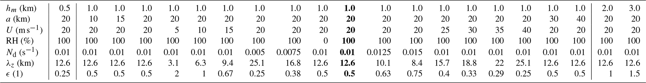
For the default scenario with the 1 km high and 20 km wide ridge and a background state with , and RH=100 %, the vertical wavelength of hydrostatic mountain waves is and the non-dimensional mountain height is . While the listed values for λz and ϵ are valid only for dry conditions, they are employed to summarize the basic characteristics of the background state. For the witch of Agnesi ridge, the critical value for the onset of wave breaking in a dry (unsaturated) atmosphere is ϵc=0.85 (Miles and Huppert, 1969). Note that while a saturated atmosphere has been shown to increase the values of ϵ and ϵc (Jiang, 2003), wave breaking does not occur due to ϵ<ϵc. Nonetheless, other nonlinear effects, such as wave amplification, cannot be completely neglected. The combination of this sounding and topography is therefore suitable as an indicator of how well the ICAR solution approximates scenarios in which nonlinearities occur, a situation ICAR is very likely to encounter in real-world applications. To this end an ICAR-N simulation is compared to a WRF simulation employing the same topography and sounding.
3.3 Analytical solution
ICAR calculates the perturbations to the horizontal background wind with Eq. (1) and Eq. (2), while the vertical wind speed is calculated according to Eq. (8). Perturbations to the potential temperature and microphysics species fields, on the other hand, result from advection and microphysical processes calculated with numerical methods. In ICAR-O this introduces a time dependency for N and, in turn, for the wind field perturbations that depend on N as input variable. Furthermore, ICAR assembles the wind field with an algorithm that allows for a spatially variable background state (Gutmann et al., 2016). It is therefore necessary to ascertain how well the exact analytical perturbations are reproduced by ICAR. This cannot be inferred from a direct comparison to WRF since the wind field of the latter is influenced by nonlinear processes not modeled by ICAR. For the topography given in Sect. 3.2 linear-theory-based analytical expressions for the resulting perturbations to a horizontally and vertically uniform background state have been derived as follows (e.g., Smith, 1979):
with u′ as the perturbation to the horizontal background wind U, w′ the perturbation to the vertical wind speed, θ′ the perturbation to the background potential temperature Θ, as the gravitational acceleration, l the Scorer parameter defined as and A(z) as the elevation-dependent amplitude of the perturbations. A(z) is given by
where ρ is the height-dependent air density of the background state. However, since the underlying equations employed by ICAR neglect the effect of wave amplification due to decreasing density with height, the term in Eq. (21) is set to unity in the following.
3.4 Boundary conditions at the model top
In this study the effect of the boundary conditions (BCs) imposed by ICAR at the upper boundary of the simulation domain is investigated. To this end several alternative BCs to the existing zero-gradient boundary condition are added to the ICAR code, their abbreviations, mathematical formulation and their numerical implementation are summarized in Table 2. All BCs constitute Neumann BCs except for the zero-value Dirichlet BC. Per default ICAR imposes a ZG BC at the model top to all quantities, corresponding to the assumption that, e.g., the mixing ratio of hydrometeors qhyd above the domain is the same as in the topmost vertical level. A zero-value (ZV) BC imposed on, e.g., qhyd avoids any advection from outside of the domain into it. The constant-gradient (CG), constant-flux (CF) and constant-flux-gradient (CFG) BCs assume that either the gradient, flux or flux gradient of ψ, respectively, remains constant at the model top, representing different physical situations. The respective discretizations of the equations given in Table 2 then determine the value of .
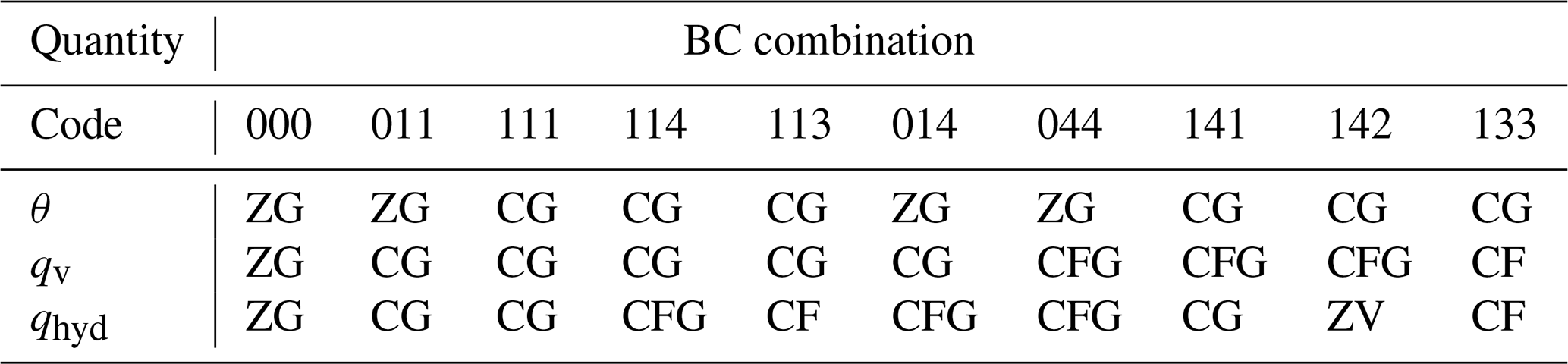
For this study, options are added to the ICAR code that allow the application of different BCs to water vapor, potential temperature and the hydrometeors (cloud water, ice, rain, snow and graupel), hereafter referred to as a set of boundary conditions. To indicate which BCs were applied to what group in a specific model run, the runs are labeled with a three-digit code; see Table 3. The first digit indicates the BC imposed on θ, the second digit the BC imposed on qv and the third digit the BC imposed on qhyd, which encompass all remaining MP species (qc, qi, qr, qs and qg). The number ID associated with each BC is listed in Table 2. In this notation, for instance, 014 denotes a simulation imposing a zero-gradient BC to θ, a constant-gradient BC to qv, and a constant flux gradient BC to the hydrometeors qhyd.
The 10 combinations of BCs tested in the sensitivity study are listed in Table 3. While a much larger set of combinations of BCs exists, physically not meaningful BC combinations, such as a zero-value BC imposed on potential temperature, were ruled out beforehand. Additionally, to reduce the parameter space further, a preliminary study was conducted to exclude sets of BCs that yielded results with distinctly higher errors than the standard zero-gradient BC.
Table 2Overview of all types of boundary conditions that were imposed at the model top of ICAR in the sensitivity study. The table lists the ID number, the abbreviation used in this study, the full name and equation of the BC evaluated at z=ztop, and the resulting equation for required to calculate the flux at the top boundary of the domain in Eq. (16). Note that the zero-gradient BC is a special case of the constant-gradient BC and that the constant c is chosen as . Due to the upwind advection scheme each BC is only applied if .
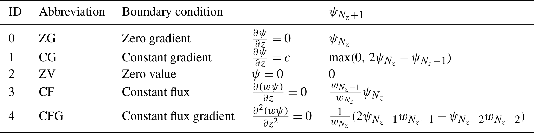
Table 3Combinations of BCs tested in the sensitivity study with idealized simulations. Each column represents a combination of three BCs used in a specific simulation. Each digit of the three-digit code refers to the ID number of a specific BC listed in Table 2 that was applied to one of the three quantities listed in the rows below. For all combinations of BCs, simulations for all of the topographic settings and background conditions listed in Table 1 were performed.
3.5 Evaluation
All evaluations conducted in this study focus on cross sections along the west–east axis of the domain, oriented parallel to the background flow. Since ICAR does not currently support periodic boundary conditions, the ICAR domain is extended along the south–north axis to minimize influences from the boundaries (see Sect. 3.1). Additionally, for ICAR the four centermost west–east cross sections from the south–north axis in the domain are averaged, and the average is found to be representative of the domain center in preliminary tests (not shown). In WRF the central west–east cross section from the south–north axis is used.
The effect of the Brunt–Väisälä frequency calculation method is investigated with a comparison of the u′ and w′ fields obtained from ICAR-N and ICAR-O simulations to the fields given by the analytical expressions in Eqs. (18) and (19). Nonlinear effects on the wind field are investigated by a comparison of ICAR to WRF. Differences between the models' and the analytical solution are quantified with the bias (B) and the mean absolute error (MAE, Wilks, 2011b, chap. 8). Since WRF uses a different model grid than ICAR, WRF fields are linearly interpolated to the ICAR grid for this comparison.
For the evaluation in this study the mixing ratios of the microphysics species are assigned to three groups: water vapor qv, suspended hydrometeors and precipitating hydrometeors . The total mass of water vapor Qv, suspended hydrometeors Qsus and precipitating hydrometeors Qprc is calculated as
where Nx and Nz are the horizontal and vertical number of grid cells, respectively, V the grid cell volume, qij(t) the mixing ratio of the respective hydrometeor species, and ρij(t) is the density of dry air within the grid cell. Note that in contrast to WRF the grid cell volume in ICAR is constant and all vertical levels have the same height Δz.
The sensitivity of the physical processes simulated by ICAR-N to the elevation of the upper boundary and the imposed boundary conditions (BCs) is inferred from the total mass of the MP species in the cross section and the spatial distribution of potential temperature, the MP species and the 12 h accumulated precipitation P12 h. Except for P12 h, all quantities are averaged over the 12 h period after a spinup of 18 h when an approximately steady state is reached. P12 h is the precipitation accumulated over the same period.
Differences in the spatial distribution of time-averaged quantities , P12 h and time-averaged total mass of the MP species with respect to the reference simulation are quantified with the sum of squared errors (SSE). The SSE is calculated between ICAR simulations with different values of ztop and the reference simulation employing the default zero-gradient BCs at the upper boundary where ztop is zmax=20.4 km. This model top is high enough that cloud processes within the troposphere are not affected by the model top. The SSE is calculated over all vertical levels, defined in both simulations as
Here is the time-averaged value of a quantity ψ in an ICAR simulation at grid point (i,j) with the model top at ztop and the set of upper BCs, and is the value of a quantity at the same location in the reference simulation with ztop=zmax. For 12 h accumulated precipitation a one-dimensional version of equation (23), with the summation only along the x axis, is employed while for total mass no summation is necessary and only the squared difference is calculated. The SSE is preferred over the mean squared error (MSE) since different model top settings result in different domain sizes, potentially favoring simulations with higher model tops due to the larger area that the errors are averaged over. While the SSE conversely tends to favor smaller domains, lower SSEs obtained for simulations with higher model tops are then a stronger indicator that increasing the model top effectively reduces errors.
To quantify the improvement of one simulation, with a set of boundary conditions BCs and model top ztop, over another by choosing a different set of boundary conditions, BCs′, at the upper boundary or another model top elevation , the reduction of error (RE) measure is employed (Wilks, 2011a, chap. 8). It is given by
This way, RE can be interpreted as a percentage improvement due to the alternative choice of or BCs′ over the original settings ztop and BCs, with RE=0 corresponding to no improvement and RE=1 corresponding to a complete removal of errors.
To characterize the effect of increasing the model top elevation on the SSE while keeping the set of boundary conditions unchanged, RE is evaluated for increasing values of between 4.4 and 14.4 km with ztop=4.4 km and in Eq. (24). The resulting RE values then are equivalent to the percentage change of the SSEs achieved by increasing ztop in comparison to the lowest tested model top setting. Similarly, to investigate the effect of an alternative set of boundary conditions, RE is evaluated for and . Here the resulting RE values quantify the percentage improvement of the SSEs achieved by changing the imposed boundary conditions at the upper boundary while leaving the model top elevation unchanged.
The quantity zmin(ψ,BCs) is introduced, which defines the model top elevation for a given set of boundary conditions BCs and parameter ψ for which RE exceeds 95 % for the first time and remains above that threshold for ztop≥zmin. In preliminary studies, the 95 % threshold value was found as a suitable indicator for reaching a saturation in error reduction (not shown). The lowest possible model top elevation Zmin is then calculated as the maximum of zmin(ψ,BCs) for all quantities ψ and a specific combination of boundary conditions BCs. However, θ is excluded since this study focuses mainly on hydrometeors. Nonetheless any relevant error in θ influences the MP fields and the distribution of precipitation, thereby directly affecting Zmin. In this context Zmin can then be interpreted as the lowest possible model top elevation such that the cloud and precipitation processes in the domain are sufficiently independent from influences of the model top.
3.6 Case study
To investigate the effects of the suggested modifications to ICAR on the distribution of precipitation for a real-world application, a case study is conducted for the Southern Alps on the South Island of New Zealand located in the southwestern Pacific Ocean. Furthermore, the procedure to identify the lowest possible model top elevation Zmin, as described in Sect. 3.5, is applied to this real case scenario and the result compared to the optimal model top elevation of 4 km found by Horak et al. (2019) for this region. In their study the model top elevation was chosen as the elevation that led to the lowest MSEs between simulated and measured 24 h accumulated precipitation for 11 sites in the Southern Alps. Section 4.6 additionally investigates whether this seemingly optimal result, as suggested by the lowest MSEs, was achieved due to the low model top potentially influencing the microphysical processes within the domain and the calculation of N being based on the perturbed fields. To this end, the hydrometeor and precipitation distribution along cross sections through the Southern Alps are compared.
To maintain comparability to Horak et al. (2019), the ICAR simulations for ICAR-O and ICAR-N are forced with the ERA-Interim reanalysis (ERAI, Dee et al., 2011) instead of the more recent ERA5 reanalysis. For the ICAR-O simulation the model top is set to 4 km, the elevation that was identified as seemingly optimal in Horak et al. (2019) and ZG BCs are applied to θ and all microphysics species (BC code 000). For the ICAR-N simulation Zmin is determined for the day of the case study as described in Sect. 3.5 by conducting multiple simulations with model tops between 5–20 km. A ZG BC is imposed on the potential temperature field to avoid numerical instabilities arising for a CG BC due to strongly stratified atmospheric layers and a CG BC is imposed on the microphysics species (BC code 011). The remaining setup for ICAR-O and ICAR-N, such as the forcing data set and the model domain, have been described in detail in Horak et al. (2019).
The case study focuses on 6 May 2015 LT (local time), a day with stably stratified large-scale northwesterly flow throughout the troposphere impinging on the Southern Alps over a 24 h period. Upstream of the South Island, ERAI exhibits a 24 h averaged relative humidity of more than 80 % in the lowest 2 km of the atmosphere, an averaged moist Brunt–Väisälä frequency of 0.012 s−1, a mean near-surface temperature of 16.5 o C and a mean specific humidity at the surface of 11 g kg−1.
4.1 Comparison to the analytical solution
Figure 1 shows the horizontal and vertical perturbations to the background state, as well as the isentropes of the perturbed potential temperature field as calculated with the analytical solution based on linear theory and simulated with ICAR-N, ICAR-O and WRF up to an elevation of 15 km. ICAR-N and ICAR-O simulations were run with ztop=20.4 km and zero-gradient boundary conditions (BC code 000). The simulations are conducted for a 2-D ridge and the default scenario with the modification that RH=0 % (see Sect. 3.2).
Generally, the horizontal west–east and vertical perturbations to the background state calculated by ICAR-N reproduce those obtained from the analytical expressions well (cf. Fig. 1a–b and e–f). The range of values of u′ in ICAR-N is −8.4 to 8.2 m s−1 compared to the −10.0 to 10.0 m s−1 derived from the analytical expression. Whereas for the north–south perturbations, the analytical solution yields , and ICAR-N calculates an average magnitude of 0.02 m s−1. The minimum and maximum of v′ are −1.6 and 1.5 m s−1 respectively, localized in close proximity to the western and eastern domain boundaries. Along the domain center, v′ lies between −0.5 and 0.5 m s−1. For w′, values obtained with ICAR-N lie between as opposed to for the analytical solution. The mean absolute error (MAE) in relation to the analytical solution of u′ is 0.9 m s−1, which corresponds to 11 % of the absolute perturbation maximum. For w′ the MAE is 0.027 m s−1 or 2 % of the absolute perturbation maximum. This indicates a smaller error in the w′ field in ICAR-N in contrast to the u′ field. In comparison to the analytical fields (Fig. 1a) the u′ field in ICAR-N exhibits slightly lower values of u′, particularly visible in the region where from approximately 8 km upward, resulting in higher horizontal wind speeds in this region (Fig. 1b). The isentropes in ICAR-N are overall very similar to those calculated analytically (see Fig. 1a–b), yielding an MAE of 0.26 K.
The wind and potential temperature fields simulated by ICAR-O (Fig. 1c, g) exhibit clear differences to the analytical solution, especially above an elevation of about 6 km. The deterioration increases with elevation and is clearly visible from approximately z=8 km upward, particularly for w′ (Fig. 1g) but is still well pronounced for u′ and the isentropes (Fig. 1c). This is reflected in slightly elevated MAEs in comparison to ICAR-N with 1.0 m s−1 in u′, 0.034 m s−1 in w′ and 0.32 K in θ. The reason for the relatively small difference to the MAEs of ICAR-N is that the MAE calculation across the entire cross section averages out the large deviations in the small spatial area around the topographical ridge at the center.
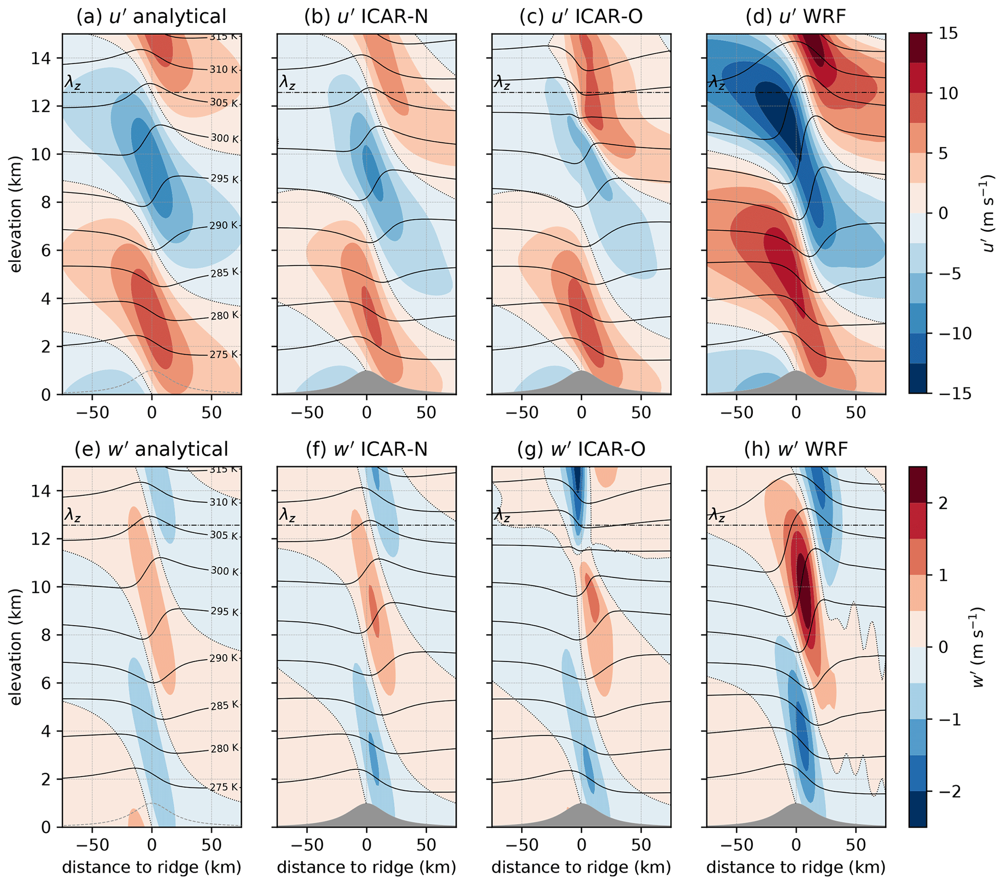
Figure 1Vertical cross sections of the horizontal perturbation wind component u′ (top row) and vertical perturbation wind component w′ (bottom row) calculated analytically (left column) and calculated by ICAR-N (second column), ICAR-O (third column), and WRF (right column). The dashed–dotted horizontal line shows the vertical wavelength of the two-dimensional hydrostatic mountain wave λz, the dotted curve shows the 0 m s−1 contour line and the solid black contour lines show the isentropes. For panel (a) and (e), where the perturbation field is evaluated on constant height levels starting at z=0 m, the topography is indicated by the dashed curve as to not obscure the perturbation field. All simulations are conducted for a 2-D ridge with hm=1 km and a=20 km and a background state with , and RH=0 %.
WRF is not expected to perfectly reproduce the analytical solution due to the occurrence of nonlinearities for the chosen non-dimensional mountain height of ϵ=0.5 and the amplification of perturbations due to the decrease in density with height. Furthermore, the occurrence of partial wave reflections from the model top is not entirely mitigated despite the careful selection of a damping layer (see Sect. 3.1). However, the WRF simulation serves as an indicator to what degree ICAR is able to capture the results obtained with a full physics model. As expected, the WRF simulation shows a larger deviation from the analytical wind field (cf. Fig. 1a, e with Fig. 1d, h). The amplitudes in the perturbation fields in WRF are larger and exhibit the elevation dependence indicated by Eq. (21). For w′, for instance, the amplitude increases by 0.7 m s−1 from 4 to 10 km, resulting in an increased orographic lift compared to ICAR. The range of observed values for u′ is −14.8 to 14.6 m s−1 and values of w′ lie between −1.7 and 2.4 m s−1. These larger maximum values in comparison to the analytical solution can mainly be attributed to the amplification of the perturbations due to the exponential decrease in density with height. For instance, at the elevation of the w′ maximum (Fig. 1h), the pressure has dropped to about one-third of the surface pressure. According to the pressure amplification term in Eq. (21) this increases the amplitude by a factor of 1.7. The remaining difference of 0.7 m s−1 is most likely caused by wave amplification due to nonlinearities and wave reflections at the damping layer. However, the general characteristics of the perturbation fields, such as the periodicity of the perturbations with elevation and the approximate location of the positive and negative perturbations, are similar to that of their corresponding analytical counterparts. The increase in the amplitude of the perturbations due to the exponential decrease in density with height continues up until approximately 15 km (not shown), above which the dampening effects of the damping layer become increasingly noticeable.
4.2 Sensitivity to the set of upper boundary conditions
Figure 2a–e show the reduction of error (RE) achieved for ICAR-N simulations for a given model top elevation ztop by applying different upper boundary conditions than the ICAR default (BC code 000). RE values are largest when a CG BC is chosen for θ (Fig. 2a), more dependent on ztop for qv (Fig. 2b) and smallest for the remaining quantities (Fig. 2c–e) with similar results for all tested topographies and the respective time-averaged total masses , and (not shown). Most tested BC combinations reduce the error in at least one of the investigated quantities, but generally not for all, with the exception of the combinations 141 and 142. However, in the case of qsus, qprc, and P12 h no improvements for any BC combination are observed once ztop>4.4 km (Fig. 2c–e). The water vapor field shows improvements for all BCs except for a CF BC, with the largest REs found for a CG BC imposed on qv. For the hydrometeors and P12 h the improvement at the lowest model top setting of 4.4 km is only found if a CFG BC is applied to water vapor and either a CG, ZV or CFG to qhyd, otherwise the RE is approximately zero.
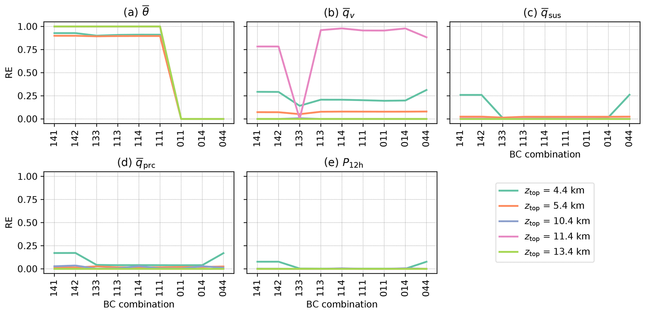
Figure 2The reduction of error (RE), dependent on the chosen combination of boundary conditions (x axis; see Table 3 for the key to the BC combination code), for (a) potential temperature , (b) water vapor , (c) suspended hydrometeors , (d) precipitating hydrometeors and (e) the 12 h precipitation sum P12 h. Note that overbars denote the temporal average of the respective quantity over 12 h following 18 h of model spinup. REs were calculated between an ICAR-N simulation with an alternative set of boundary conditions imposed at the upper boundary and an ICAR-N simulation employing the standard zero-gradient boundary condition (BC code 000), both run with the same model top elevation ztop (indicated by line color). All simulations are conducted for the default scenario.
The choice of an alternative BC over the standard ZG BC has the largest potential for a reduction of error when (i) the grid cells of the uppermost vertical level coincide with regions of vertical convergence where w<0 and and (ii) the vertical flux gradients ϕz in these regions are negative (see Sect. 2.2.2). Note that this particularly requires ψ>0. For potential temperature, in case of the specified sounding, all conditions are always satisfied in some region no matter at what elevation the model top is chosen; see Fig. 3a, where the vertical flux gradient of the potential temperature divided by the local potential temperature, given by , is shown. Consequently θ exhibits the largest reductions of error across all values of ztop with only a small dependence on ztop (see Fig. 2a). For water vapor, as shown in Fig. 2b, RE as a function of ztop exhibits two peaks, the first at ztop=4.4 km and the second at ztop=11.4 km, with a minimum in between. Here the exponential decay of qv with height results in comparatively small values for ϕz(qv) above an elevation of 4 km (not shown). However, still exhibits minima and maxima at higher elevations due to the periodicity of the vertical velocity field (see Fig. 3b). At the locations of these minima and maxima of the relative error introduced by a boundary condition can therefore be large as well. In the case of qv, as shown in Fig. 3b, the model top of a simulation with ztop=11.4 km would coincide with a downdraft region of strong vertical convergence and negative close to the domain center, implying strong water vapor flux convergence. The same situation occurs for ztop=4.4 km albeit in a region with a lower value of and weaker vertical convergence. Therefore, the local change in qv due to a mass influx caused by the boundary condition is comparatively small, resulting in a lower relative error. Note that for simulations with the vertical convergence in downdraft regions at the model top is weaker and is lower. Therefore, as shown in Fig. 2b, the RE achieved for qv exhibits two peaks where the RE is high for the lowest model top setting at 4.4 km, exhibits a maximum at ztop=11.4 km and is low otherwise.
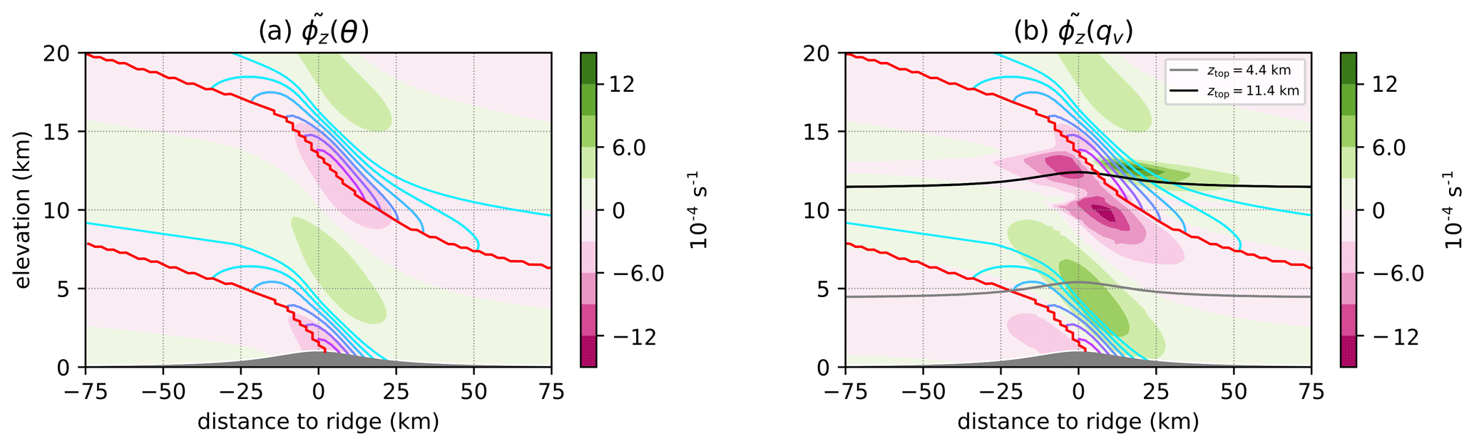
Figure 3The normalized vertical flux gradient of (a) potential temperature and (b) water vapor (see the text for further description). The values are calculated from an ICAR-N simulation at t=30 h with ztop=20.4 km and ZG BCs (000) for the default scenario. The contour lines indicate the vertical convergence () in regions were . Here the violet contour lines represent stronger vertical convergence and the teal contour lines weaker vertical convergence in the range between and 0 s−1 spaced in increments of . The red contour line indicates where . In panel (b), gray and black lines additionally indicate the location of the model top for ztop=4.4 km and ztop=11.4 km, respectively.
For the investigated scenarios, altering the boundary condition applied to θ has only a negligible effect on the microphysics species fields and P12 h. This is observed, for instance, for simulations 011 and 111 where the BC applied to θ was changed from a ZG to CG while the BCs imposed on the MP species remained the same: both BC settings lead to very similar RE values for the MP species (Fig. 2b–d) and P12 h (Fig. 2e) despite the RE drop observed for (Fig. 2a). This is due to the location of the errors that are introduced with the standard ZG BC on θ. As shown in Fig. 4, for simulations with higher model tops these are mainly confined to the topmost kilometer of the model domain. If ztop is set high enough these deviations therefore do not affect the cloud processes below. A potential reason for this behavior is that air that is either too warm or cold, depending on the error introduced by the BC, is advected into the topmost vertical level. From there it is redistributed by vertical and horizontal advection until an equilibrium is reached, effectively confining the introduced errors to the topmost vertical levels of the domain. While the results indicate that a CG BC effectively reduces errors in θ, it is found to be problematic for atmospheres with stronger stratifications. For the 1 km high and 20 km wide witch of Agnesi ridge and a background state of RH=100 %, and , ICAR-N simulations began to exhibit numerical instabilities. These were triggered by the CG BC causing the upper levels of the model domain to heat up, an issue not observed for the ZG BC (not shown).
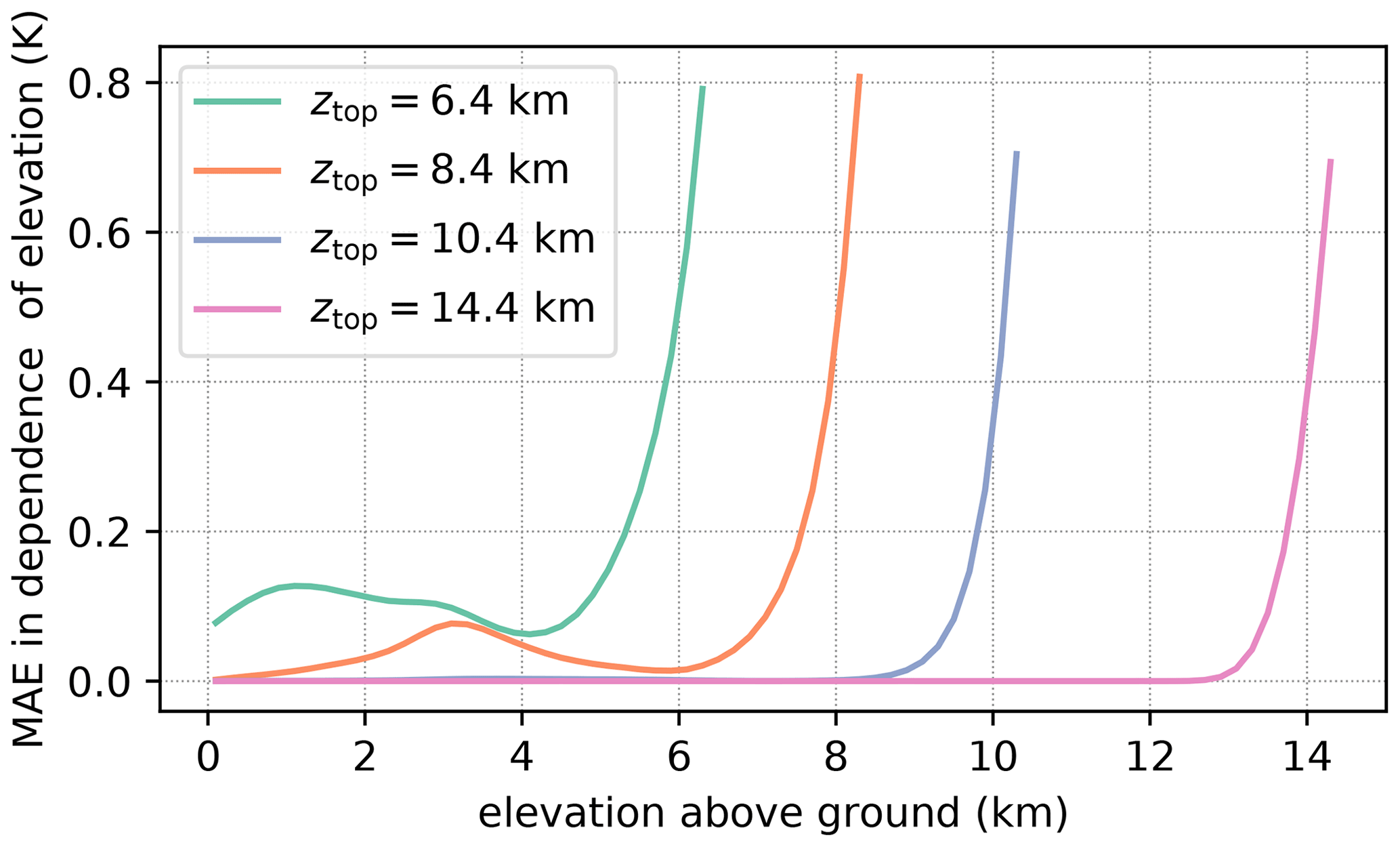
Figure 4The mean absolute error (MAE) of potential temperature in ICAR-N simulations employing ZG BCs (000) with different model top settings ztop that are dependent on the elevation above ground (x axis). The MAE is calculated with respect to a reference simulation with ztop=20.4 km and ZG BCs (000). All simulations are conducted for the default scenario.
Figure 5a–b shows that the model top elevation necessary for a RE of 95 %, zmin(ψ,BCs), is essentially constant and therefore independent of the imposed BCs for all investigated quantities except for potential temperature. Imposing a CG BC on θ at the upper boundary lowers zmin(Θ,BCs) from 12.4 to 9.4 km. Similar results are found for ICAR-N simulations conducted for the other tested topographies (not shown). To reduce the parameter space in the following analysis, and since the results for each BC combination are very similar, the idealized simulations from here on focus on CG BCs imposed at the model top (BC code 111). This combination is chosen over the others for its computational simplicity, the larger REs observed for and , as well as the potential to reduce zmin(θ,BCs) in the idealized simulations.
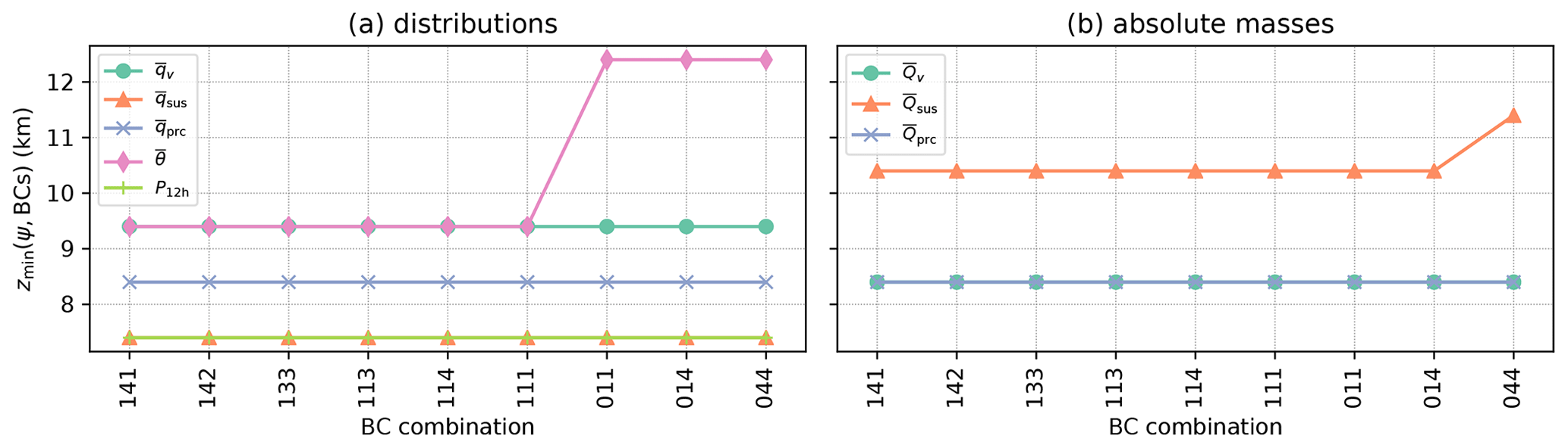
Figure 5The panels show the minimum model top elevation zmin(ψ,BCs) necessary to reduce the error by 95 % for (a) water vapor , suspended hydrometeors , precipitating hydrometeors , potential temperature , and the 12 h precipitation sum P12 h and (b) the total mass of water vapor , suspended hydrometeors , and precipitating hydrometeors , dependent on the set of upper boundary conditions. The ICAR-N simulations are run for the default scenario.
4.3 Sensitivity to the model top elevation
As shown in Fig. 6a–g, for most investigated quantities the reduction of error (RE) increases monotonously with the model top elevation ztop for all tested topographies. Once the threshold of 95 % is exceeded, further increases in ztop correspond to distinctly lower increases in RE. However, non-monotonic exceptions exist as, for instance, the total mass of water vapor shown in Fig. 6e. Here exhibits a local maximum at ztop=5.4 km, before dropping to lower values that eventually converge towards RE=1. This is a direct consequence of the influence of the model top on the cloud processes within the domain, which for the investigated scenarios is particularly pronounced for suspended hydrometeors qsus. For ICAR-N simulations conducted for the default scenario (BC code 111) with increasing values of ztop, Fig. 7a shows the cloud boundary of suspended hydrometeors. Here it is defined as the contour line where . While the upwind cloud adjacent to the ridge occupies a large region in the simulations with the lowest model tops, it initially shrinks with increasing ztop until a minimum extension is reached at ztop=7.4 km. After this minimum the cloud increases in size with higher ztop. The extension of a smaller secondary cloud upwind of the ridge decreases in size similarly before it vanishes completely for ztop≥8.4 km. Conversely, downwind of the ridge at an elevation of approximately 6 to 9 km a larger cloud forms only for ztop≥6.4. Altogether, the total mass of suspended hydrometeors, shown in Fig. 7b, initially decreases with increasing ztop until a local minimum at 6.4 km is reached. In the simulation with this model top elevation, less water vapor is converted into suspended hydrometeors qsus, leading to a local maximum of at ztop=6.4 km (Fig. 7b). This specific behavior is found independently of the imposed boundary conditions and results in the same cloud boundaries as shown in Fig. 7a. If a different witch of Agnesi ridge configuration is employed, the same shrinking of the qsus cloud occurs with increasing ztop; however, in these simulations the cloud boundaries differ from those in Fig. 7a (not shown).
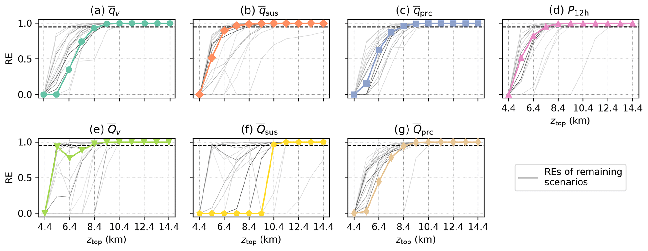
Figure 6The reduction of error (RE), dependent on ztop evaluated for the time-averaged distribution of (a) water vapor , (b) suspended hydrometeors , (c) precipitating hydrometeors , and (d) 12 h precipitation sum P12 h and the time-averaged total masses of (e) water vapor , (f) suspended hydrometeors , and (g) precipitating hydrometeors . The colored curves show RE(ztop) of the respective quantity in the ICAR-N simulations conducted for the default scenario, while the gray curves indicate the RE of simulations for the other scenarios. The ICAR-N simulations imposed CG BCs on all quantities at the upper boundary (BC code 111). The dashed black line shows the 95 % RE threshold.
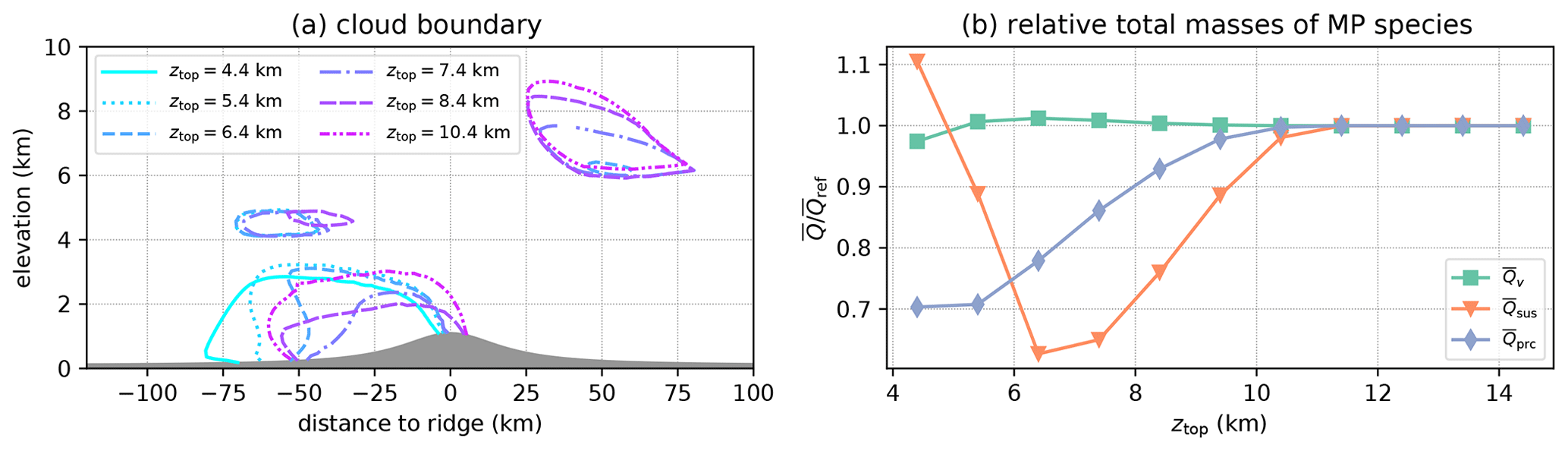
Figure 7Panel (a) shows the boundary of a suspended hydrometeor cloud defined by the contour line for ICAR-N simulations with different model top elevations after 30 h of simulation. Panel (b) shows the mean total mass of the microphysics species in ICAR-N simulations, dependent on ztop and normalized with their respective mass in a reference simulation with ztop=20.4 km. The ICAR-N simulations are run for the default scenario with CG BCs imposed on all quantities at the upper boundary (BC code 111).
Note that the spread of RE dependent on ztop (Fig. 6) for , , and P12 h is mainly caused by scenarios that generate clouds with large vertical extensions. To better approximate the microphysical processes in the scenarios and the resulting distribution of precipitation, higher model tops are required, leading to the observed spread. This affects , and in particular, since missing vertical levels may significantly impact the total masses. In addition, note that while total masses are always compared to the respective mass found in the reference simulations, , and can only be compared within the vertical extent simulated by the simulation with the lower model top.
The results show that the total masses of the microphysics species alone are not sufficient to determine whether the processes within the domain are influenced by the model top. In other words, the spatial distribution of these quantities needs to be taken into account as well. Conversely, even though the error in the distribution of is reduced by at least 95 % once a model top elevation of 7.4 km is employed, the same occurs for the total mass only at ztop=10.4 km (cf. Fig. 6b, f). Therefore, both the distribution of a quantity and its total mass are necessary to reliably determine whether the cloud formation processes within the domain is independent from influences of the model top. Overall, the results show that for the default scenario a lowest possible model top elevation of Zmin=10 km is required for ICAR-N to represent cloud processes undisturbed from the influence of the upper boundary of the domain. Furthermore, the value of Zmin is found to depend strongly on the specific scenario simulated, with values ranging from 8–14 km.
4.4 The lowest possible model top elevation
This section investigates how the lowest possible model top elevation Zmin depends on ridge height hm and width a, as well as the background state employed in the ICAR-N simulations. Note that Zmin is defined as the maximum of zmin(ψ,BCs) and thereby represents the model top elevation required for a 95 % reduction of error in all quantities (except θ) for a given set of boundary conditions (BC code 111 in the following). For a background state with and , the results indicate a weak dependence of Zmin on the ridge height, with higher Zmin for higher ridges (Fig. 8a). The dependency of Zmin on the width of the ridge, on the other hand, exhibits no distinct pattern (Fig. 8b).
For a witch of Agnesi ridge with hm=1 km and a=20 km, Zmin exhibits a clear dependence on the background state as shown in Fig. 8c. In the following, the background state is characterized by the vertical wavelength of the resulting mountain wave in dry conditions, given by . Note that the characteristics of the results remained unchanged (not shown) even if instead of Nd the mean moist Brunt–Väisälä frequency Nm in the lowest kilometer of the atmosphere (e.g., Jiang, 2003) is employed to calculate λz. In Fig. 8c λz is varied either by keeping constant and varying U or by fixing and varying Nd. Figure 8c shows that Zmin decreases with increasing vertical wavelength. A potential reason for this behavior is that lower λz corresponds to a higher number of periods of updrafts and downdrafts within the troposphere. This increases the likelihood that the model top passes through a region with convergent downdrafts and a negative vertical flux gradient ϕz, thereby triggering the mass-influx mechanism outlined in Sect. 2.2.2. At high enough model top elevations all quantities (except for θ), and in turn ϕz(ψ), eventually tend towards zero, and any influence of the model top on the cloud and precipitation processes in the model domain becomes negligible. For longer vertical wavelengths another effect could come into play. Here model top elevations at approximately may become feasible due to the minimum of the vertical wind speeds at this height. For wavelengths larger than approximately 10 km the results are similar and do not depend on whether the longer wavelength is obtained by an increase in U or by decreasing Nd while keeping the other variable constant. However, they exhibit clear differences at shorter wavelengths. While at shorter wavelengths Zmin decreases gradually as λz increases due to increasing U, the decrease in Zmin is distinctly steeper if the longer wavelength is obtained by lowering Nd. The majority of the steeper decrease is explicable with the CG boundary condition chosen for θ, which causes numerical instabilities for .
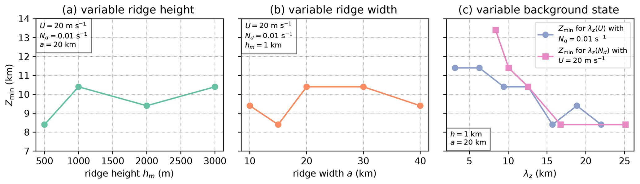
Figure 8The dependence of the lowest possible model top elevation Zmin on (a) ridge height with constant ridge width of 20 km, (b) ridge width with constant ridge height of 1 km, and (c) vertical wavelength λz of hydrostatic mountain waves where λz is adjusted either by changing U or Nd for a ridge with hm=1 km and a=20 km. The ICAR-N simulations are conducted with CG BCs imposed on all quantities (BC code 111).
4.5 Comparison to WRF
This section compares the spatial distribution of water vapor qv, suspended hydrometeors qsus, precipitating hydrometeors qprc and 12 h sum of precipitation P12 h calculated by ICAR-N to the corresponding fields in WRF. ICAR-N imposes CG BCs (111) and employs a model top elevation of ztop=10.4 km. This is the lowest possible model top elevation Zmin required for a 95 % reduction of error in all quantities for the chosen set of BCs determined for the default scenario. The distributions of qv, qsus and qprc are investigated after 30 h of simulation time, while P12 h is investigated between 19 and 30 h of simulation time. The comparison aims to highlight the differences that may be expected between an ICAR-N and WRF simulation due to the tradeoff between physical fidelity and model performance. The scenario is chosen such that the wind field is expected to exhibit nonlinearities.
4.5.1 Water vapor and hydrometeors
With respect to water vapor ICAR-N is drier upwind of the topographical ridge and wetter downwind in comparison to WRF (see Fig. 9a–c). The regions with this dry and wet bias extend up to an elevation of approximately 6 km in which ICAR-N exhibits slightly stronger updrafts than WRF up to 200 km upwind of the ridge. This stronger orographic lift in ICAR-N yields a higher conversion rate of water vapor to hydrometeors. On the other hand, above the ridge the downdrafts calculated by WRF are of a higher magnitude than those predicted by ICAR-N; see Fig. 10c and d. Here, WRF advects drier air from higher elevations to lower levels. Hence, the two large regions in ICAR-N exhibiting a dry and wet bias in qv, respectively, are likely caused by the differences in the wind field. Additionally, a small region with a wet bias close to the ridge slope on the windward side is presumably caused by microphysical conversion processes (Fig. 10c). Here the stronger orographic lifting in WRF leads to a higher microphysical conversion rate of qv to hydrometeors, thereby resulting in the observed wet bias of ICAR-N in terms of qv. Above the downwind slope of the ridge and up to approximately 100 km downwind, the downdrafts in WRF are still stronger than in ICAR-N. This potentially causes an increased conversion of hydrometeors to qv by evaporation, resulting in the dry bias of ICAR-N in this region. This low level dry bias is likely increased by ICAR-N, overall, extracting more precipitation from the moist atmosphere than WRF (see Sect. 4.5.2).

Figure 9Mixing ratios (color contours) of water vapor (a, b, c), suspended hydrometeors (d, e, f) and precipitating hydrometeors (g, h, i) calculated with ICAR-N (a, d, g), WRF (b, e, h) and the difference between ICAR-N and WRF (c, f, i) after 30 h of simulation. The isentropes of ICAR-N and WRF are shown as gray contour lines with 3 K increments. The direction of the background flow is from left to right. Note that the scaling of the contours for all quantities is nonlinear to reveal details in the respective distributions. ICAR-N and WRF simulations are conducted for the default scenario with ICAR-N imposing CG BCs on all quantities at the upper boundary (BC code 111).
Clear differences between the ICAR-N and WRF simulations are observed for suspended hydrometeors. While the approximate shape of the windward cap cloud (Fig. 9d and e) shows similarities, the mixing ratios calculated by ICAR-N are approximately one-tenth of those in WRF (see Fig. 9f). Furthermore, the main constituent of the cap cloud in ICAR-N is ice qi, while it is liquid water qc in WRF (not shown).
The majority of precipitating hydrometeors in ICAR-N are observed windward of the topographical ridge, extending over most of the upwind slope (Fig. 9g). In WRF, on the other hand, the distribution of qprc is centered above the ridge and extends farther downwind than upwind (Fig. 9h). In both models the majority of qprc consists of snow qs (not shown). However, WRF additionally predicts non-negligible amounts of graupel qg up to 20 km upwind of the ridge (not shown). Altogether, for precipitating hydrometeors (Fig. 9i) ICAR-N is wetter on the windward slope but drier above the ridge and the downwind slope. This is caused by a combination of two factors: (i) the higher vertical wind speeds above the windward slope of the topographical ridge predicted by WRF lead to lower effective falls speeds of the hydrometeors (see Fig. 10d), and (ii) higher horizontal wind speeds additionally contribute to a larger horizontal drift of qprc and precipitation spill-over in WRF (see Fig. 10b and, for a basic estimation of the drift distances, Sect. 4.5.2).
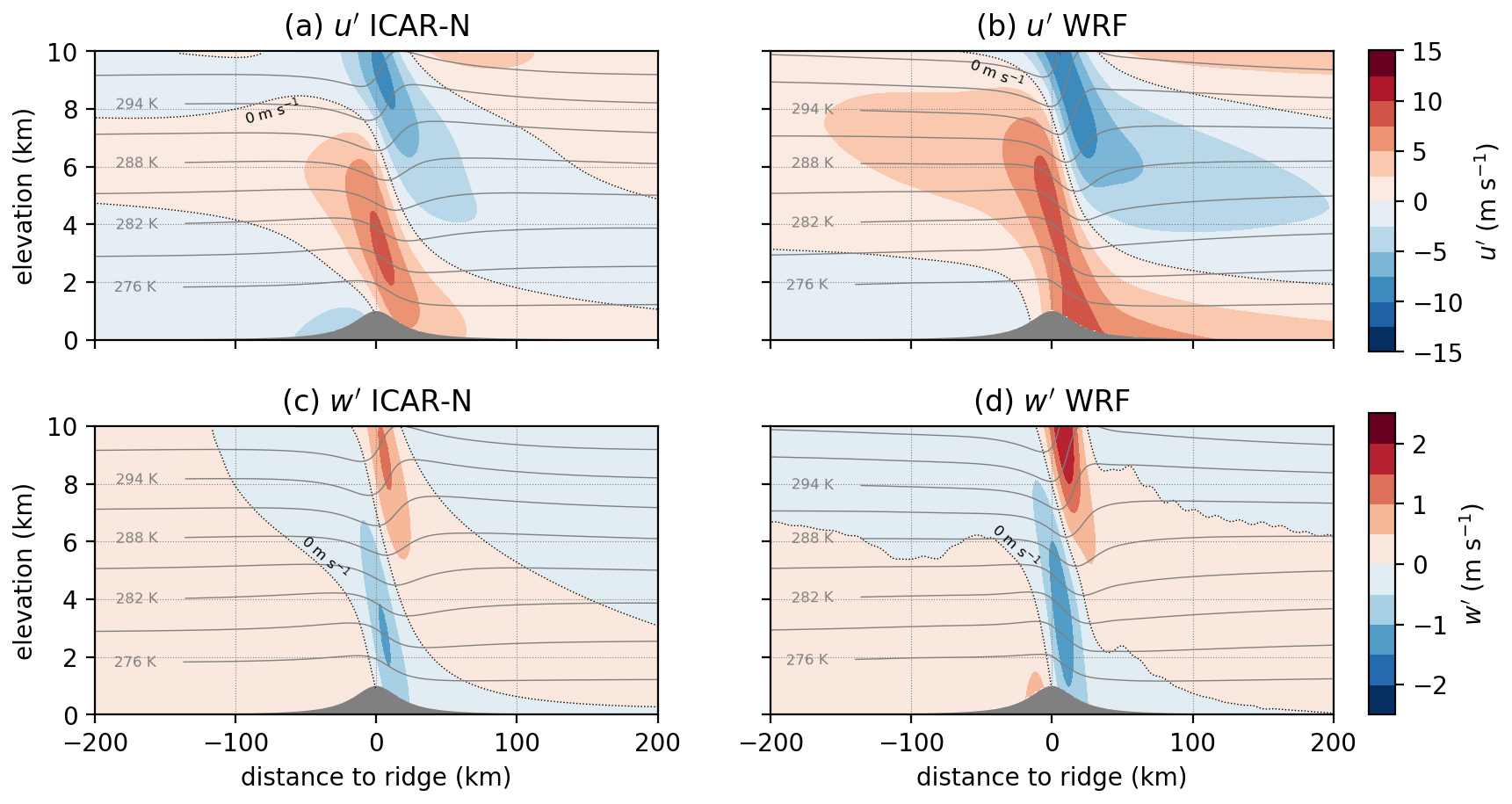
Figure 10Perturbations of the horizontal wind component u′ (a, b) and vertical wind component w′ (c, d) calculated by ICAR-N with ztop=10.4 km (a, c) and WRF (b, d). The dotted curve shows the 0 m s−1 contour line and the black lines indicate the isentropes. Both simulations are run for the default scenario with ICAR-N imposing CG BCs on all quantities at the upper boundary (BC code 111).
4.5.2 Precipitation
Figure 11a illustrates that P12 h on the windward slope is substantially higher in ICAR-N than in WRF and that, conversely, ICAR-N is drier along the leeward slope. This corresponds well to the distribution and shape of the precipitating hydrometeors above the windward and leeward slope (see Fig. 9g and h) and the differences of qprc between ICAR-N and WRF (see Fig. 9i). The precipitation maximum predicted by ICAR-N is approximately 25 mm and lies 6 km upwind of the ridge peak in comparison to the 32 mm maximum in WRF, which lies 4 km upwind of the ridge (Fig. 11a). The median of P12 h, however, is located upwind of the ridge peak in ICAR-N and downwind in WRF, separated by a distance of 20 km (see Fig. 11b). Integration along the cross section shows that 63 % of ICAR-N precipitation falls out upwind of the domain center, while for WRF it is only 43 %.
The distribution of precipitation in ICAR-N is asymmetric with a gradual increase until the maximum is reached and a steeper decrease after that. While in WRF P12 h is asymmetric as well, the distribution exhibits a very steep increasing slope ending in a distinct peak that is followed by a decreasing slope comparable to the decrease of P12 h in ICAR-N. In WRF snow and graupel contribute to P12 h, while the precipitation in ICAR-N is solely composed of snow. The graupel shower predicted by WRF is localized within a 30 km region centered approximately 10 km upwind of the ridge and causes the distinct peak observed in the distribution of precipitation in WRF (Fig. 11a).
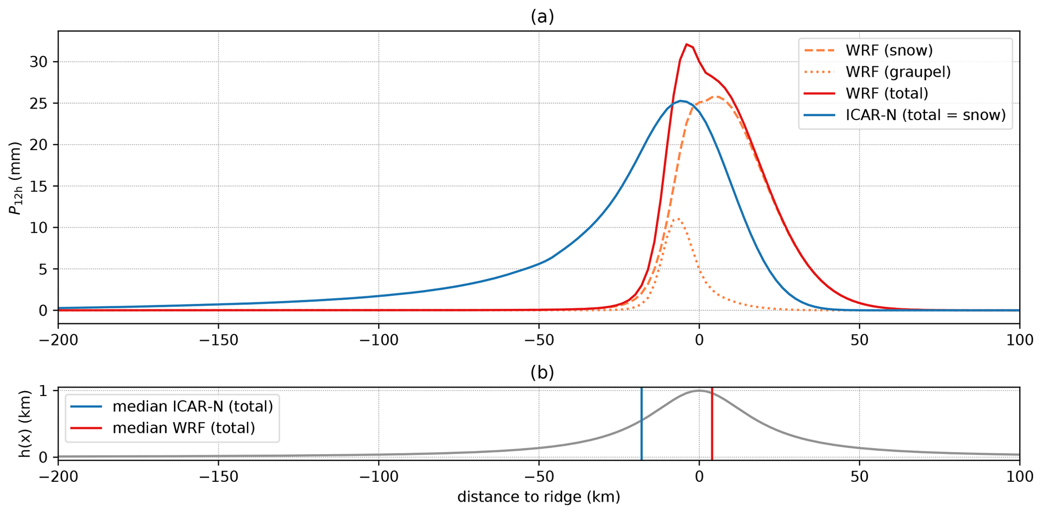
Figure 11(a) The 12 h accumulated total precipitation P12 h along the cross section for ICAR-N (solid blue curve) and WRF (solid red curve). Additional curves indicate the contribution of graupel (dotted orange curve) and snow (dashed orange curve) to the total precipitation of WRF. ICAR-N total precipitation consists solely of snow, i.e., rain and graupel are zero in this specific simulation. (b) topography along the cross section with vertical blue and red lines indicating the locations of the medians of the total precipitation distribution of ICAR-N and WRF respectively. Both models are run for the default scenario, while ICAR-N imposes CG BCs on all quantities at the upper boundary (BC code 111).
The maximum of accumulated snow in WRF is 48 mm and the median of the distribution is shifted downstream by 22 km in relation to the median of the precipitation distribution in ICAR-N, which is solely snow. The difference is mainly due to the different wind fields of ICAR-N and WRF. In the following a fall speed for snow in stagnant air of is assumed for the ICAR-N and WRF simulations alike. Starting 1 km above the orography, the effective fall speeds in ICAR-N and WRF are −0.75 and respectively, based on an average w′ above the upwind slope of the ridge of 0.25 m s−1 in ICAR-N and 0.75 m s−1 in WRF (see Fig. 10c–d). In combination with an approximate average horizontal wind speed of 17.5 m s−1 in ICAR-N and 21 m s−1 in WRF (Fig. 10a–b), this results in a difference in the resulting horizontal drift of 19 km, which fits the observed difference in the medians of the accumulated snow precipitation distribution well. Hence, the discrepancy in the precipitation distribution appears to be mainly caused by an underestimation of the perturbation velocities in ICAR.
The absence of graupel in ICAR-N compared to WRF can be traced to the MP scheme and is a result of the atmospheric conditions it encounters. The Thompson MP predicts graupel formation if riming growth exceeds the depositional growth of snow (Thompson et al., 2004). While the necessary atmospheric conditions are easily satisfied in WRF, the cloud water mixing ratio in ICAR-N is too low to initiate sufficient riming growth (see Fig. 9d). However, no clear indication for the underlying cause of the large difference in the cloud water mixing ratios between ICAR-N and WRF is found.
4.6 Case study
The previous sections have demonstrated that (i) the Brunt–Väisälä frequency needs to be diagnosed from the background stratification in order to model a realistic perturbation flow field with ICAR, that (ii) it further requires a minimum model top elevation (which is dependent on the orography and the atmospheric background state), and that (iii) a combination of ZG and CG BCs (BC codes 011 and 111) are optimal to be used at the top of the ICAR model domain. The effects of these suggested modifications to ICAR on a real-world application are investigated with a case study conducted for the Southern Alps on the South Island of New Zealand located in the southwestern Pacific Ocean (Fig. 13a).
The Southern Alps are a mountain range approximately 800 km long and 60 km wide. They are oriented southwest–northeast and extend from approximately 41 to 46∘ S, with approximately 97 % of the crest line lying above an elevation of (meters above mean sea level) and the highest peaks rising above . The mean precipitation regime in the humid and maritime climate on the South Island of New Zealand is strongly influenced by the orography of the Southern Alps. The prevailing westerly and north-westerly winds advect moist air against the topographic barrier, leading to a precipitation maximum of approximately 14 m yr−1 along its western flanks in close proximity to the alpine ridge. While the western coast on average receives 5 m yr−1, the plains east of the alpine ridge receive at most 1 m yr−1 due to the precipitation shadow of the Southern Alps (Griffiths and McSaveney, 1983; Henderson and Thompson, 1999).
For this region two ICAR-O and one ICAR-N simulations are conducted. ICAR-O calculates the Brunt–Väisälä frequency N based on the perturbed state of the atmosphere and imposes ZG BCs to all quantities (BC code 000). The model tops are set to 4 km (ICAR-O4 km) and 15.2 km (ICAR-O15.2 km), respectively, where the lower elevation was determined as optimal in Horak et al. (2019) by comparing 24 h accumulated precipitation to observations. ICAR-N, on the other hand, calculates N from the forcing data set and imposes a zero-gradient BC on the potential temperature field and constant-gradient BCs on the microphysics species (BC code 011). The lowest possible model top elevation Zmin with an acceptably low error is determined by applying the method outlined in Sect. 3.5 based on multiple ICAR-N simulations with model top elevations between 5–20 km (Fig. 12). The resulting value of Zmin is found at 15.2 km, which is in stark contrast to the value of 4 km in Horak et al. (2019). This indicates that the cloud formation processes in the ICAR-O simulation with the low model top elevation are likely unphysical and strongly disturbed by the model top.
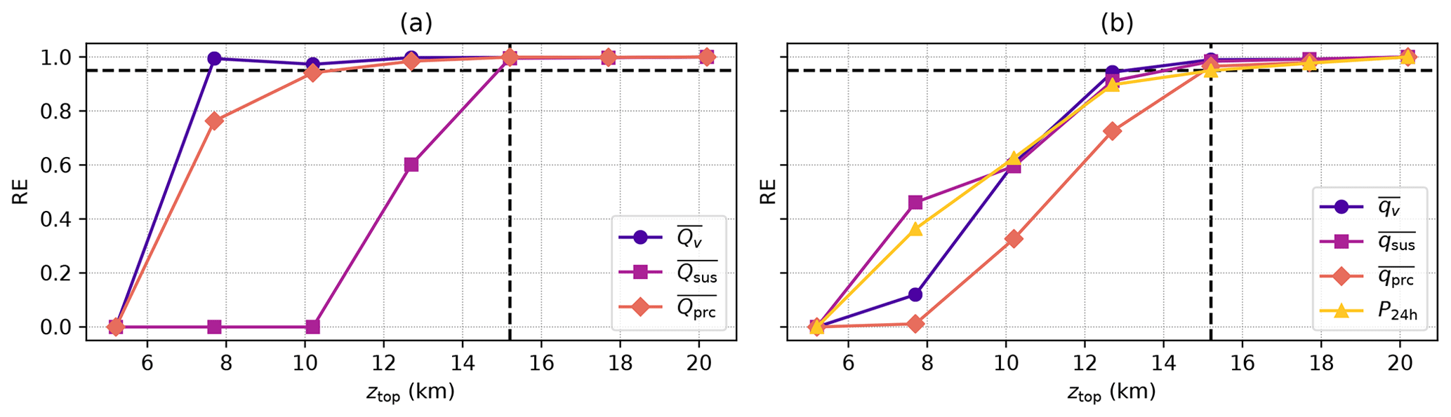
Figure 12The reduction of error (RE) of the simulations for the South Island of New Zealand for (a) the total mass of the MP species in the domain, and (b) the distribution of the MP species and precipitation dependent on the model top elevation ztop. ICAR-N imposes a ZG BC on the potential temperature field and constant-gradient BCs on the microphysics species (011). The dashed horizontal line indicates the 95 % RE threshold used to determine Zmin, and the dashed vertical line shows at which model top this threshold is exceeded for all quantities.
The resulting patterns of P24 h for ICAR-N and the ICAR-O simulations on the South Island of New Zealand are shown in Fig. 13b, c and e, while the differences between ICAR-N and ICAR-O are shown in Fig. 13d and f, respectively. Overall the precipitation patterns produced by ICAR-N and both ICAR-O simulations are very similar with a maximum approximately at the western flanks of the Southern Alps. However, while ICAR-N and ICAR-O4 km produce similar precipitation maxima, albeit shifted spatially upwind in ICAR-N, the maximum amount is lower in ICAR-O15.2 km (compare Fig. 13b, c and e). ICAR-N is clearly drier in regions above and downwind of the alpine range when compared to ICAR-O4 km (Fig. 13d). This is still observed in comparison to ICAR-O15.2 km, although to a lesser extent (Fig. 13f). Conversely, ICAR-N generates the majority of its precipitation in close proximity to the coast and, compared to both ICAR-O simulations, is wetter in the regions upwind of the western slopes of the Southern Alps (Fig. 13d and f). The reason for ICAR-O4 km producing precipitation further downwind than ICAR-N can be found in the cross sections of hydrometeor distributions shown in Fig. 14.
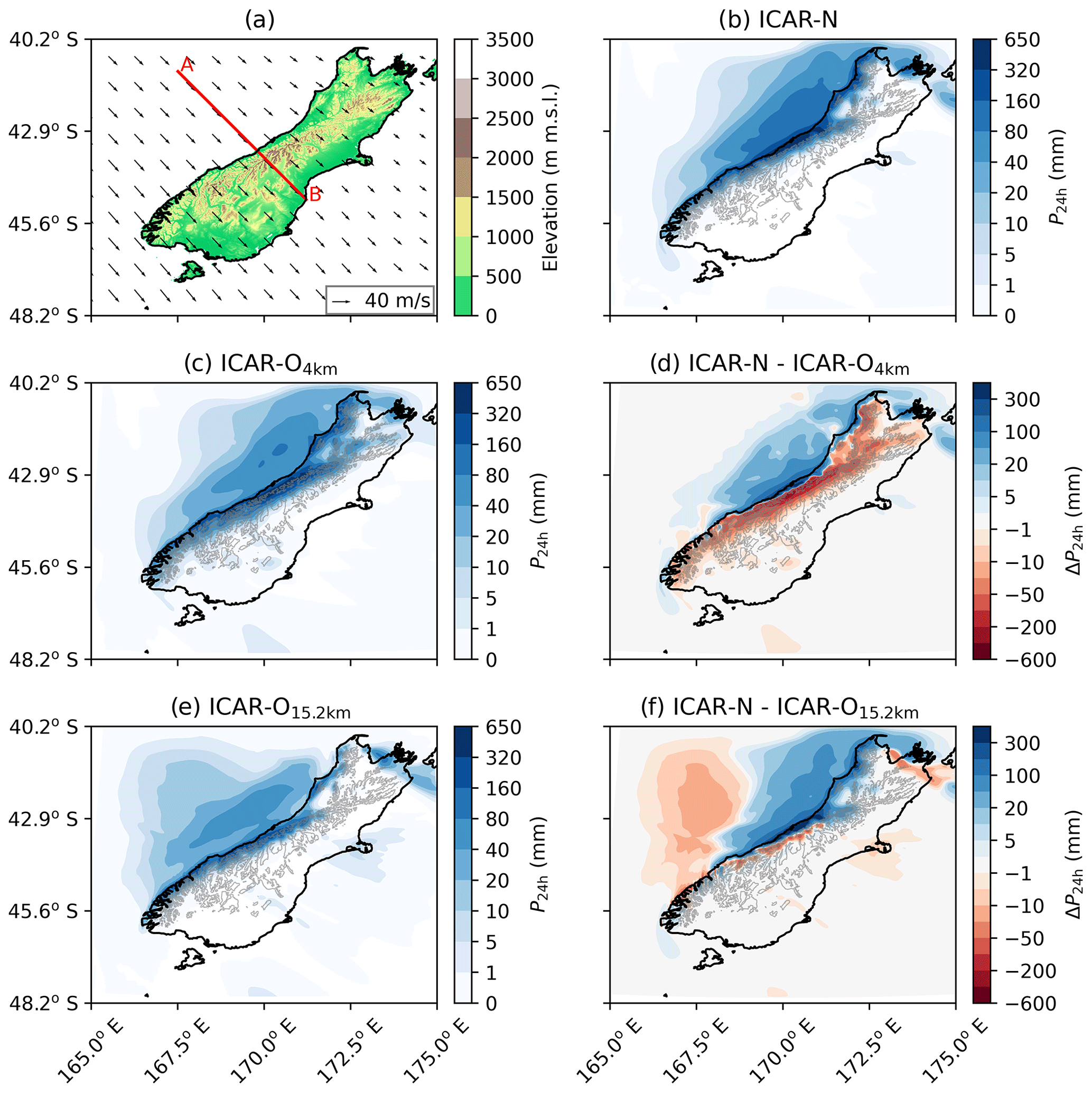
Figure 13(a) The South Island of New Zealand study domain with the horizontal wind field at the 500 hPa level and the location of the vertical cross section (red line), (b) P24 h pattern for ICAR-N with ztop=15.2 km and a ZG BC imposed on θ and CG BCs imposed on the MP species (BC code 011), (c) P24 h pattern for ICAR-O with ztop=4 km imposing ZG BCs (BC code 000), (d) difference in 24 h accumulated precipitation P24 h between ICAR-N and ICAR-O4 km, (e) P24 h pattern for ICAR-O with ztop=15.2 km imposing ZG BCs (BC code 000), and (f) difference in 24 h accumulated precipitation P24 h between ICAR-N and ICAR-O15.2 km on the 6 May 2015 LT. Panels (b)–(f) additionally show the contour line of the topography.
Clear differences can be observed in the distributions of (Fig. 14a and c). Note the distinct maximum of above the initial topography peak in ICAR-O4 km, which is almost entirely absent in ICAR-O15.2 km and ICAR-N. These maxima occur in the topmost levels of the ICAR-O4 km domain and suggest that the ZG BC overestimates the moisture content of the atmospheric column and artificially introduces additional water into the domain (as outlined in Sect. 2.2.2). This leads to the formation of artificial clouds downwind of approximately 169.8∘ E. Furthermore, this indicates that the formation of these artificial clouds can be mitigated just by increasing the model top elevation. Note that in ICAR-N (Fig. 14c) the cloud formation is confined to a region upwind of 169.8∘ E.
Furthermore, this artificial cloud in ICAR-O4 km near the model top generates precipitating hydrometeors that extend farther to the lee of the alpine crest compared to ICAR-O15.2 km and ICAR-N (Fig. 14d–f). ICAR-O15.2 km additionally exhibits a considerably lower amount of precipitating hydrometeors compared to ICAR-O4 km and ICAR-N (Fig. 14e). While ICAR-N produces more precipitation overall and is wetter than ICAR-O4 km on the initial ramp of the western slope of the alpine range (up to approximately 169.8∘ E in Fig. 14i), ICAR-O4 km is wetter downwind, yielding higher amounts of precipitation at the peak and the first leeward slope (Fig. 14i). The distribution of P24 h ICAR-O15.2 km is similar to that of ICAR-O4 km but with lower amounts and a lesser extent downwind (Fig. 14i). Note that ICAR-O4 km produces clouds in the topmost model levels even farther downstream as well (Fig. 14a); however, they do not generate precipitating hydrometeors during the investigated period. Note that for this case study the effect of raising the model top elevation is mainly the removal of artificial clouds in the topmost model levels (compare Fig. 14a and b) and a weakening of the updrafts upwind of the initial peak in the topography (not shown), yielding a lower concentration of (compare Fig. 14d and e). Calculating the Brunt–Väisälä frequency from the atmospheric background state instead of the perturbed state of the domain, on the other hand, results in stronger updrafts and increased amounts of and P24 h (compare Fig. 14e and f and Fig. 14h and i).

Figure 14Cross sections along the South Island of New Zealand (line A–B in Fig. 13a) for an ICAR-O simulation (ztop=4.0 km, BCs 000, a, d, g), an ICAR-O simulation (ztop=15.2 km, BCs 000, b, e, h) and an ICAR-N simulation (ztop=15.2 km, BCs 011, c, f, i). The panels show the 24 h averaged mixing ratio of suspended hydrometeors (a, b, c), precipitating hydrometeors (d, e, f), and the 24 h accumulated precipitation, as well as the difference in precipitation between ICAR-N and the respective ICAR-O simulation (g, h, i).
These results strongly indicate that the low model top setting of 4 km employed in Horak et al. (2019) is inadequate to allow for a correct representation of the cloud and precipitation processes within the domain despite the relatively high skill found for ICAR-O4 km in their study. Therefore, the results additionally demonstrate that when model skill is evaluated with statistical metrics based on surface observations alone (Horak et al., 2019), it does not necessarily reflect the skill of the model in correctly representing atmospheric processes such as gravity waves and associated cloud formation. Hence, it seems that the underestimation in precipitation near the crest and to its lee in an ICAR simulation with a reasonably high model top compared to WRF (Fig. 9) is partly compensated in an ICAR simulation with a too low model top (ICAR-O4 km in Fig. 14) by spurious effects introduced by the upper boundary conditions. Note that this seeming improvement is not due to a more realistic representation of cloud formation processes.
The results highlight that a more accurate representation of the wind fields is obtained only when the Brunt–Väisälä frequency, in accordance with linear mountain wave theory, is calculated from the unperturbed background state of the atmosphere (ICAR-N) rather than from the perturbed state (ICAR-O). The remaining differences of the wind fields in ICAR-N to the analytical solution may be attributable to two causes: firstly, to solve the governing equations ICAR numerically calculates the Fourier transform of the topography h(x,y) in the domain. In cases where h(x,y) is not constant along the domain boundaries or where it exhibits discontinuities within the domain, this approach gives rise to numerical artifacts (see the Gibbs phenomenon, e.g., Arfken et al., 2013), introducing errors into the perturbed fields. Note that for a 2-D ridge as employed in this study, . Therefore, while , with xw and xe the x coordinate of the western and eastern domain boundary, respectively, h(x)≠const along the northern or southern domain boundary. This results in an average value of v′ of 0.02 m s−1 instead of the expected 0 m s−1 and therefore slightly altered values of u′ and w′ in comparison to the results from linear theory. These issues may be reduced by, for instance, filtering the topography accordingly or by adding a buffer around the domain (Florinsky, 2016). Additional research is necessary to determine which filtering methods or modifications to the topography are best suited to preprocess digital elevation models for ICAR. Secondly, ICAR solves for w′ according to Eq. (8) and only analytically calculates u′ and v′.
ICAR is intended as a computationally frugal alternative to full physics models, in principle allowing for very low model top elevations. While employing a low model top to take advantage of the associated computational cheapness is tempting, increased efficiency should not come at the cost of the physical fidelity of the model. The results in this study clearly show that there is a lowest possible model top elevation Zmin that ensures that the physical processes within the domain are not influenced by the model top. Boundary conditions imposed on qv and the hydrometeors at the upper boundary are found not to influence the value of Zmin for the investigated parameter space despite potentially mitigating errors in the potential temperature and water vapor fields. Specifically, the cloud formation and precipitation processes within the domain are shown to almost exclusively depend on the model top elevation ztop and not on the chosen set of boundary conditions and only stabilize for ztop≥Zmin. It seems unlikely that any boundary condition is able to accurately represent the effect of cloud and precipitation processes above the model domain and the resulting interaction with the corresponding processes in the model domain (e.g., the seeder–feeder mechanism). Therefore, in order to capture all relevant cloud and precipitation processes, it is recommended that the vertical extension of the domain should at the very least encompass the entire troposphere. Altogether these results highlight that model top elevations within the troposphere, as employed by past studies, are to be avoided (e.g., Gutmann et al., 2016; Horak et al., 2019; Alonso-Gónzalez et al., 2020).
This study strongly suggests that no general value for Zmin is applicable to all possible scenarios, with the results exhibiting large differences between the idealized simulations and the real case study. For the tested parameter space, including the real case, Zmin mainly depends on the background state and the height of the topography. The dependence on the background state, characterized by the vertical wavelength of the hydrostatic mountain wave, shows that overall larger λz results in smaller Zmin and, conversely, smaller λz results in larger Zmin. The dependence of Zmin on the background state is explicable with the horizontal wind speed U and the Brunt–Väisälä frequency N affecting the location, amount, and magnitude of the updraft and downdrafts in the domain. Similarly, Zmin depends on ridge height due to the generally stronger updrafts and downdrafts triggered by higher topographies; see Eq. (19). However, note that the dependence on the ridge height is weak compared to the dependence on the background state.
The determination of Zmin considers all MP species with respect to their time-averaged spatial distribution and the time-averaged total mass within the cross section as well as the 12 h (P12 h, idealized simulations) or 24 h (P24 h, real case simulations) precipitation sum along the cross section. Note that potential temperature θ is indirectly included in determining Zmin since errors in the θ field influence the cloud formation and precipitation processes. However, this study shows that errors in the θ field introduced by the zero-gradient boundary condition are mainly localized in the topmost vertical levels (Fig. 4), which correspond to approximately the uppermost 1 to 2 km of the domain and result in only a negligible influence on cloud formation processes in the tested parameter space. While a constant-gradient boundary condition reduces the errors in the potential temperature field, the default zero-gradient boundary condition is a suitable alternative for θ provided ztop is high enough. This can be ensured by, for instance, employing the method to determine Zmin described in this study.
A comparison between ICAR-N and WRF simulations conducted for the same topography and sounding reveals substantial differences in the spatial distributions of qv, qsus, and qprc, as well as the resulting P12 h. These differences are mainly attributable to additional effects included in the WRF but not the ICAR-N wind field, such as nonlinearities and the amplification of the perturbations due to the density decreasing with height. However, not all reasons for the differences could be identified, and results remain inconclusive as to why ICAR-N mainly produces cloud ice while it is cloud water in WRF. Overall, both models predict the occurrence of distinctly different events: a snow shower with the majority of snow falling upwind of the ridge in ICAR-N and a snow and graupel shower in WRF with the largest portion precipitating leeward of the ridge. While these results are obtained for one specific sounding, they indicate that the linearization of the wind field has the potential to significantly alter the distribution of precipitation in a study domain. This could have drastic consequences for the results of studies relying on ICAR to provide precipitation fields for, e.g., applications in hydrology or glaciology. Future work could implement and investigate whether the amplification of perturbations (see Eq. 21) due to the vertical density gradient yields ICAR-N results closer to those of WRF. Another conceivable avenue for future investigations in that regard could be the implementation and evaluation of a set of linear wave equations derived from the anelastic equations into ICAR-N.
For strongly stratified atmospheric conditions, a constant-gradient BC was found to cause numerical stability issues in the idealized and real case simulations alike. Future studies could investigate further BC options that might allow a better approximation of the potential temperature profile: such approaches might, for instance, (i) analytically diagnose θ for the vertical level above the model top and then apply the corresponding values as a Dirichlet BC or (ii) prescribe the potential temperature from the corresponding height in the forcing data set as Dirichlet BC at the model top in ICAR. Another possible venue for future research that aims to mitigate the influence of the upper boundary could be the implementation of a relaxation layer directly underneath the model top. In this layer perturbed quantities could, as they approach the model top, gradually be relaxed towards their background state values, while w is relaxed towards zero.
The case study investigates the effect of the proposed modifications to ICAR on a real-world application for the South Island of New Zealand. It reveals that these modifications shift the distribution of precipitation upwind, leading to drier conditions in the alpine range but wetter coastal regions. The method for the determination of Zmin presented in this study does not rely on tuning to measurements and may therefore be employed for every region in the world for which a suitable digital elevation model and atmospheric forcing data are available. Furthermore, the method ensures that for ztop=Zmin the cloud formation processes within the domain are independent from influences of the model top and that only the absolutely necessary amount of vertical levels is used in the simulations. This preserves as much of the computational efficiency of ICAR as possible without sacrificing additional physical fidelity. However, the extension of the method to determine Zmin to longer study periods, compared to the 24 h of the case study, and a larger variety of background states is not trivial and outside the scope of this study. If a substantial amount of simulations for different background states is required to determine Zmin, the associated computational cost may outweigh the gain of employing the lowest possible number of vertical levels for the entire study period. Therefore, future research could investigate variations of the Zmin determination employed in this study. For instance, a focus on the background states most frequent during each season or on background states with shorter vertical wavelengths (resulting in higher values of Zmin) to find upper bounds for Zmin may drastically reduce the required number of simulations.
With regard to the case study, the unmodified version of ICAR (ICAR-O) is found to produce enhanced precipitation in the alpine range due to artifacts (heightened mixing ratios of hydrometeors) in the topmost vertical levels in the horizontal vicinity of topographical peaks. This additionally caused the very low model top elevation found with the method employed in Horak et al. (2019): at each alpine weather station on the South Island of New Zealand Horak et al. (2019) calculated a mean squared error (MSE) between the simulated and measured precipitation accumulated over 24 h (P24 h) at alpine sites. The artifacts in the topmost vertical levels of ICAR-O (with ztop=4 km) lead to an increase in precipitation at these alpine sites in comparison to ICAR-N or, as noted by Horak et al. (2019), to ICAR-O simulations with higher model top elevations. Since all ICAR-O simulations generally underestimate precipitation amounts at alpine weather stations on the South Island of New Zealand, and overshooting of measured values mostly does not occur, the higher amounts of P24 h for the simulation with ztop=4 km then lowered the calculated MSE. Even though the atmospheric processes in the ICAR-N simulation are more correctly represented in comparison to ICAR-O, the lower amount of P24 h at the alpine sites would result in a higher MSE. Therefore, even though the calculated MSEs were lowest for a model top setting at 4 km, the seemingly correct results were produced for the wrong reasons. This additionally exemplifies why comparisons to isolated measurements alone cannot determine whether the model results are correct for the correct reason. Only a detailed consideration of the underlying processes can be the basis for such a conclusion.
The key findings and recommendations based on the extensive process-based evaluation of ICAR are summarized in the following.
-
There is a minimum possible model top elevation Zmin to produce physically meaningful results with ICAR. If the model top elevation is lower, cloud formation and precipitation processes within the domain are affected by the model top.
-
Results show that in order to avoid spurious influences of the upper boundary to the microphysical processes within the domain, Zmin should be at least as high as the tropopause but may be required to be even higher in other situations.
-
Determining an exact value for Zmin from comparisons to precipitation measurements may yield results in closer agreement to these measurements but potentially for the wrong reasons (i.e., model artifacts).
-
The method described in this study to determine Zmin may be applied to idealized simulations and real cases alike. This was demonstrated as a proof of concept.
-
While most of the tested boundary conditions (in comparison to the default zero-gradient boundary condition) are suitable to reduce the errors in the water vapor and potential temperature fields, no tested combination of these boundary conditions results in a lower value for Zmin.
-
Model skill, when inferred only from comparisons to surface observations, does not necessarily reflect the model skill in representing atmospheric processes.
-
The representation of the wind field in ICAR is improved by ensuring that the Brunt–Väisälä frequency is calculated from the background state of the atmosphere provided by the forcing data. Note that the current version of ICAR employs the perturbed state of the domain.
This study highlights the importance of a process-based in-depth evaluation not only with respect to ICAR but for models in general. Particularly for regional climate models (RCMs) and numerical weather prediction (NWP) models, the results of the case study demonstrate a potential pitfall when model parameters are inferred solely from comparisons to measurements, potentially leading to situations for which model results are more prone to be right but for the wrong reasons. With the increasing complexity of RCMs and NWPs, ICAR could provide a computationally frugal framework to study and better understand singular model components. This would allow for a process-based evaluation of, e.g., MP schemes or advection schemes, contributing to the development and improvement of RCMs and NWPs.
The modified version ICAR v1.0.1 employed for the simulations (https://doi.org/10.5281/zenodo.4042993, Gutmann et al., 2020), as well as the results obtained (Horak, 2020), are available at https://doi.org/10.5281/zenodo.3609953.
The investigation and its design, the simulations and their analysis, and the visualization of the results and writing (original draft and editing) were carried out by JH. The conceptualization of the paper was a joint effort from all authors, as were the discussion and refinement of the methods presented. Additionally, funding acquisition and project administration were carried out by MH.
The authors declare that they have no conflict of interest.
The computational results have been achieved with the high-performance computing support from Cheyenne (https://doi.org/10.5065/D6RX99HX) provided by NCAR's Computational and Information Systems Laboratory, sponsored by the National Science Foundation, and with the HPC infrastructure LEO of the University of Innsbruck. The following open-source libraries were employed to perform the data processing and analysis presented in this study: numpy (van der Walt et al., 2011), pandas (McKinney, 2010), xarray (Hoyer and Hamman, 2017) and matplotlib (Hunter, 2007). The authors thank Lukas Umek for his contribution to finding the best dampening layer configuration in WRF.
This research has been supported by the Austrian Science Fund (FWF) (grant no. 28006-N32).
This paper was edited by Rohitash Chandra and reviewed by three anonymous referees.
Alonso-González, E., Gutmann, E., Aalstad, K., Fayad, A., and Gascoin, S.: Snowpack dynamics in the Lebanese mountains from quasi-dynamically downscaled ERA5 reanalysis updated by assimilating remotely-sensed fractional snow-covered area, Hydrol. Earth Syst. Sci. Discuss. [preprint], https://doi.org/10.5194/hess-2020-335, in review, 2020. a
Arakawa, A. and Lamb, V. R.: Computational Design of the Basic Dynamical Processes of the UCLA General Circulation Model, in: Methods in Computational Physics: Advances in Research and Applications, edited by: Chang, J., Elsevier, Netherlands, 173–265, https://doi.org/10.1016/B978-0-12-460817-7.50009-4, 1977. a
Arfken, G. B., Weber, H. J., and Harris, F. E.: Chapter 19 – Fourier Series, in: Mathematical Methods for Physicists (Seventh Edition), edited by: Arfken, G. B., Weber, H. J., and Harris, F. E., Academic Press, Boston, 935–962, https://doi.org/10.1016/B978-0-12-384654-9.00019-0, 2013. a
Barstad, I. and Grønås, S.: Dynamical structures for southwesterly airflow over southern Norway: the role of dissipation, Tellus A, 58, 2–18, https://doi.org/10.1111/j.1600-0870.2006.00152.x, 2006. a, b, c
Bernhardt, M., Härer, S., Feigl, M., and Schulz, K.: Der Wert Alpiner Forschungseinzugsgebiete im Bereich der Fernerkundung, der Schneedeckenmodellierung und der lokalen Klimamodellierung, Österreichische Wasser- und Abfallwirtschaft, 70, 515–528, https://doi.org/10.1007/s00506-018-0510-8, 2018. a
Courant, R., Friedrichs, K., and Lewy, H.: Über die partiellen Differenzengleichungen der mathematischen Physik, Math. Ann., 100, 1432–1807, https://doi.org/10.1007/BF01448839, 1928. a
Dee, D. P., Uppala, S. M., Simmons, A. J., Berrisford, P., Poli, P., Kobayashi, S., Andrae, U., Balmaseda, M. A., Balsamo, G., Bauer, P., Bechtold, P., Beljaars, A. C. M., van de Berg, L., Bidlot, J., Bormann, N., Delsol, C., Dragani, R., Fuentes, M., Geer, A. J., Haimberger, L., Healy, S. B., Hersbach, H., Hólm, E. V., Isaksen, L., Kållberg, P., Köhler, M., Matricardi, M., McNally, A. P., Monge-Sanz, B. M., Morcrette, J.-J., Park, B.-K., Peubey, C., de Rosnay, P., Tavolato, C., Thépaut, J.-N., and Vitart, F.: The ERA-Interim reanalysis: Configuration and performance of the data assimilation system, Q. J. Roy. Meteor. Soc., 137, 553–597, https://doi.org/10.1002/qj.828, 2011. a
Doms, G. and Baldauf, M.: A Description of the Nonhydrostatic Regional COSMO-Model Part I: Dynamics and Numerics, Tech. rep., Deutscher Wetterdienst, Germany, 2018. a
Dörnbrack, A. and Nappo, C. J.: A note on the application of linear wave theory at a critical level, Bound.-Lay. Meteorol., 82, 399–416, https://doi.org/10.1023/A:1000270821161, 1997. a
Durran, D.: Mountain Meteorology|Lee Waves and Mountain Waves, in: Encyclopedia of Atmospheric Sciences, second edn., edited by: North, G. R., Pyle, J., and Zhang, F., Academic Press, Oxford, 95–102, https://doi.org/10.1016/B978-0-12-382225-3.00202-4, 2015. a, b
ECMWF: IFS Documentation CY45R1 Part III: Dynamics and numerical procedures, no. 3 in IFS Documentation, ECMWF, available at: https://www.ecmwf.int/node/18713 (last access: 15 March 2021), 2018. a
Emanuel, K. A.: Atmospheric convection, vol. 58, Oxford University Press, Oxford, England, 1994. a
Florinsky, I. V.: Chapter 5 – Errors and Accuracy, in: Digital Terrain Analysis in Soil Science and Geology, second edn., edited by: Florinsky, I. V., Academic Press, 149–187, https://doi.org/10.1016/B978-0-12-804632-6.00005-5, 2016. a
Goswami, M. and O'Connor, K. M.: A “monster” that made the SMAR conceptual model “right for the wrong reasons”, Hydrol. Sci. J., 55, 913–927, https://doi.org/10.1080/02626667.2010.505170, 2010. a
Griffiths, G. A. and McSaveney, M.: Distribution of mean annual precipitation across some steepland regions of New Zealand, New Zeal. J. Sci., 26, 197–209, 1983. a
Gutmann, E., Barstad, I., Clark, M., Arnold, J., and Rasmussen, R.: The Intermediate Complexity Atmospheric Research Model (ICAR), J. Hydrometeorol., 17, 957–973, https://doi.org/10.1175/JHM-D-15-0155.1, 2016. a, b, c, d, e, f, g, h, i, j, k
Gutmann, E., Eidhammer, T., Bohlinger, P., Horak, J., Vano, J., Rasouli, K., and Scaff, L.: johanneshorak/icar: ICAR-N (Version ICAR-N), Zenodo, https://doi.org/10.5281/zenodo.4042993, 2020. a, b
Henderson, R. and Thompson, S.: Extreme rainfalls in the Southern Alps of New Zealand, J. Hydrol., 38, 309–330, 1999. a
Horak, J.: Data set – Idealized ridge simulations with ICAR and WRF, Zenodo, https://doi.org/10.5281/zenodo.3609953, 2020. a, b
Horak, J., Hofer, M., Maussion, F., Gutmann, E., Gohm, A., and Rotach, M. W.: Assessing the added value of the Intermediate Complexity Atmospheric Research (ICAR) model for precipitation in complex topography, Hydrol. Earth Syst. Sci., 23, 2715–2734, https://doi.org/10.5194/hess-23-2715-2019, 2019. a, b, c, d, e, f, g, h, i, j, k, l, m, n, o, p, q, r, s
Hoyer, S. and Hamman, J.: xarray: ND labeled Arrays and Datasets in Python, J. Open Res. Softw., 5, 10, https://doi.org/10.5334/jors.148, 2017. a
Hunter, J. D.: Matplotlib: A 2D Graphics Environment, Comput. Sci. Eng., 9, 90–95, https://doi.org/10.1109/MCSE.2007.55, 2007. a
Jarosch, A. H., Anslow, F. S., and Clarke, G. K.: High-resolution precipitation and temperature downscaling for glacier models, Clim. Dyn., 38, 391–409, 2012. a
Jiang, Q.: Moist dynamics and orographic precipitation, Tellus A, 55, 301–316, https://doi.org/10.3402/tellusa.v55i4.14577, 2003. a, b
Klemp, J. B., Dudhia, J., and Hassiotis, A. D.: An Upper Gravity-Wave Absorbing Layer for NWP Applications, Mon. Weather Rev., 136, 3987–4004, https://doi.org/10.1175/2008MWR2596.1, 2008. a
McKinney, W.: Data structures for statistical computing in python, in: Proceedings of the 9th Python in Science Conference, 1 July 2010, Austin, TX, vol. 445, pp. 51–56, 2010. a
Miles, J. W. and Huppert, H. E.: Lee waves in a stratified flow, Part 4, Perturbation approximations, J. Fluid Mech., 35, 497–525, https://doi.org/10.1017/S0022112069001248, 1969. a
Nappo, C. J.: The Linear Theory, in: An Introduction to Atmospheric Gravity Waves, Int. Geophys., 102, 29–56, https://doi.org/10.1016/B978-0-12-385223-6.00002-1, 2012. a
Oreskes, N., Shrader-Frechette, K., and Belitz, K.: Verification, Validation, and Confirmation of Numerical Models in the Earth Sciences, Science, 263, 641–646, https://doi.org/10.1126/science.263.5147.641, 1994. a
Patankar, S.: Numerical Heat Transfer and Fluid Flow, Series in computational methods in mechanics and thermal sciences, Taylor & Francis, USA, 1980. a
Popper, K.: Logik der Forschung, Springer-Verlag Wien GmbH, 1935. a
Sawyer, J.: Gravity waves in the atmosphere as a three-dimensional problem, Q. J. Roy. Meteor. Soc., 88, 412–425, https://doi.org/10.1002/qj.49708837805, 1962. a
Schlünzen, K.: On the validation of high-resolution atmospheric mesoscale models, J. Wind Eng. Ind. Aerod., 67–68, 479–492, https://doi.org/10.1016/S0167-6105(97)00095-0, 1997. a, b
Skamarock, W. C., Klemp, J. B., Dudhia, J., Gill, D. O., Liu, Z., Berner, J., Wang, W., Powers, J. G., Duda, M. G., Barker, D., and Yu Huang, X.: A Description of the Advanced Research WRF Model Version 4, Tech. rep., NCAR/UCAR, https://doi.org/10.5065/1dfh-6p97, 2019. a, b, c
Smith, R. B.: The influence of mountains on the atmosphere, Adv. Geophys., 21, 87–230, https://doi.org/10.1016/S0065-2687(08)60262-9, 1979. a, b
Smith, R. B. and Barstad, I.: A Linear Theory of Orographic Precipitation, J. Atmos. Sci., 61, 1377–1391, https://doi.org/10.1175/1520-0469(2004)061<1377:ALTOOP>2.0.CO;2, 2004. a
Stensrud, D.: Parameterization Schemes: Keys to Understanding Numerical Weather Prediction Models, Cambridge University Press, Cambridge, 2009. a
Thompson, G., Rasmussen, R. M., and Manning, K.: Explicit Forecasts of Winter Precipitation Using an Improved Bulk Microphysics Scheme. Part I: Description and Sensitivity Analysis, Mon. Weather Rev., 132, 519–542, https://doi.org/10.1175/1520-0493(2004)132<0519:EFOWPU>2.0.CO;2, 2004. a
Thompson, G., Field, P. R., Rasmussen, R. M., and Hall, W. D.: Explicit forecasts of winter precipitation using an improved bulk microphysics scheme. Part II: Implementation of a new snow parameterization, Mon. Weather Rev., 136, 5095–5115, https://doi.org/10.1175/2008MWR2387.1, 2008. a
van der Walt, S., Colbert, S. C., and Varoquaux, G.: The NumPy Array: A Structure for Efficient Numerical Computation, Comput. Sci. Eng., 13, 22–30, https://doi.org/10.1109/MCSE.2011.37, 2011. a
Warner, T. T.: Quality Assurance in Atmospheric Modeling, B. Am. Meteorol. Soc., 92, 1601–1610, https://doi.org/10.1175/BAMS-D-11-00054.1, 2011. a
Wilks, D.: Chapter 2 – Review of Probability, in: Statistical Methods in the Atmospheric Sciences, Int. Geophys., 100, 7–19, https://doi.org/10.1016/B978-0-12-385022-5.00002-6, 2011a. a
Wilks, D.: Chapter 8 - Forecast Verification, in: Statistical Methods in the Atmospheric Sciences, Int. Geophys., 100, 301–394, https://doi.org/10.1016/B978-0-12-385022-5.00008-7, 2011b. a
Zhang, D.-L., Lin, Y., Zhao, P., Yu, X., Wang, S., Kang, H., and Ding, Y.: The Beijing extreme rainfall of 21 July 2012: “Right results” but for wrong reasons, Geophys. Res. Lett., 40, 1426–1431, https://doi.org/10.1002/grl.50304, 2013. a