the Creative Commons Attribution 4.0 License.
the Creative Commons Attribution 4.0 License.
 | 05 Feb 2020
ACCESS-OM2 v1.0: a global ocean–sea ice model at three resolutions
Andrew McC. Hogg
Nicholas Hannah
Fabio Boeira Dias
Gary B. Brassington
Matthew A. Chamberlain
Christopher Chapman
Peter Dobrohotoff
Catia M. Domingues
Earl R. Duran
Matthew H. England
Russell Fiedler
Stephen M. Griffies
Aidan Heerdegen
Petra Heil
Ryan M. Holmes
Andreas Klocker
Simon J. Marsland
Adele K. Morrison
James Munroe
Maxim Nikurashin
Peter R. Oke
Gabriela S. Pilo
Océane Richet
Abhishek Savita
Paul Spence
Kial D. Stewart
Marshall L. Ward
Fanghua Wu
Xihan Zhang
We introduce ACCESS-OM2, a new version of the ocean–sea ice model of the Australian Community Climate and Earth System Simulator. ACCESS-OM2 is driven by a prescribed atmosphere (JRA55-do) but has been designed to form the ocean–sea ice component of the fully coupled (atmosphere–land–ocean–sea ice) ACCESS-CM2 model. Importantly, the model is available at three different horizontal resolutions: a coarse resolution (nominally 1∘ horizontal grid spacing), an eddy-permitting resolution (nominally 0.25∘), and an eddy-rich resolution (0.1∘ with 75 vertical levels); the eddy-rich model is designed to be incorporated into the Bluelink operational ocean prediction and reanalysis system. The different resolutions have been developed simultaneously, both to allow for testing at lower resolutions and to permit comparison across resolutions. In this paper, the model is introduced and the individual components are documented. The model performance is evaluated across the three different resolutions, highlighting the relative advantages and disadvantages of running ocean–sea ice models at higher resolution. We find that higher resolution is an advantage in resolving flow through small straits, the structure of western boundary currents, and the abyssal overturning cell but that there is scope for improvements in sub-grid-scale parameterizations at the highest resolution.
- Article
(28670 KB) - Full-text XML
-
Supplement
(46 KB) - BibTeX
- EndNote


Ocean–sea ice models have extensive applications. They form the oceanic component of coupled climate and Earth system models that are used for projecting future climate and can incorporate biogeochemical and ecosystem dynamics which extend the realm of application. They are also needed for forecasting on shorter timescales – both forecasting in the ocean and for seasonal prediction of the ocean–sea ice–atmosphere state. As a research tool, ocean–sea ice models can be used to quantitatively test, or experiment with, the dynamics of the climate system; such process studies have been invaluable in forming a broad understanding of the drivers of climate change and variability.
Modelling studies face the challenge of compromising between resolving critical processes and computational expense. For example, the standard grid spacing for the ocean component of coupled climate models is currently 1∘, with indications that some models being prepared for the next Coupled Model Intercomparison Project (CMIP6) will use 0.25∘ horizontal spacing. However, 1∘ models do not resolve the ocean mesoscale, meaning that they miss key processes that can influence the climate. Higher-resolution models usually have improvements in the climate state with better estimates of vertical heat transport (Griffies et al., 2015), enhancement of boundary currents (Hewitt et al., 2016), better resolution of ocean straits, and improved Southern Ocean state (Bishop et al., 2016). On the other hand, high-resolution simulations consume huge computational resources, which limits the length of runs and the capacity to optimize the model configuration (or minimize biases) by testing the model over a wide parameter space. There is also less experience in the coupled ocean–atmosphere–ice modelling communities in the integration of these high-resolution ocean models for climate simulations. Thus, while higher-resolution models are becoming computationally feasible, the additional resolution does not necessarily result in improved simulations.
One of the complexities in characterizing model performance as a function of resolution is the influence of model biases governing the model state. It is well-known, for example, that different models subjected to the same atmospheric state produce differing mean states (e.g. Griffies et al., 2009; Danabasoglu et al., 2014). It follows that investigating the effects of model resolution requires a clean hierarchy: a model suite in which variations in resolution are available with homogeneous code, forcing, and, as far as possible, parameter choices. This is a technique successfully employed by the DRAKKAR consortium (Barnier et al., 2014) as well as climate model developers (e.g. Griffies et al., 2015; Hewitt et al., 2016). Driving a model suite from a common prescribed atmosphere enables a relatively clean assessment of resolution dependence; however, such models will be more strongly driven by the atmosphere than coupled ocean–atmosphere models since they lack the negative feedback of sea surface temperature and currents onto the atmosphere (e.g. Hyder et al., 2018; Renault et al., 2016).
In this paper we outline the development of the latest version of the ocean–sea ice component of the Australian Community Climate and Earth System Simulation, known as ACCESS-OM2. This model was developed to serve the twin aims of underpinning climate model development and ocean state forecasting in Australia; it therefore includes the parallel development of low-, medium-, and high-resolution options. It is based on the ocean–sea ice components of the Australian Community Climate Earth System Simulator (ACCESS), which was originally formulated for coupled climate simulations (Bi et al., 2013a) and therefore designed to support Australian efforts in developing models for the upcoming Coupled Model Intercomparison Project (CMIP6). The high-resolution configuration of ACCESS-OM2 is intended for use in the next version of the Ocean Forecasting Australia Model (OFAM4), a component of the Australian Bureau of Meteorology's operational ocean reanalysis and forecasting system (Bluelink; see Oke et al., 2013, and references therein). Finally, the model suite is also intended for use in ocean and sea ice process studies and sensitivity tests.
In this paper we aim to document the model formulation (Sect. 2) and the computational performance of the model at each resolution (Sect. 3). We also undertake a preliminary evaluation of the global model state (Sect. 4.1), the circulation in selected regions (Sect. 4.2), and the model representation of sea ice (Sect. 4.3). In Sect. 5 we summarize and conclude the study.
Model configurations at three horizontal resolutions have been developed: ACCESS-OM2 (nominally 1∘ horizontal grid spacing), ACCESS-OM2-025 (nominally 0.25∘ spacing), and ACCESS-OM2-01 (nominally 0.1∘ spacing). The suite of three resolutions is also collectively referred to as ACCESS-OM2. Configurations (e.g. run parameters and forcing) are as consistent as possible across the three resolutions to facilitate studies of resolution dependence and sub-grid-scale parameterizations. The coarser models serve as test beds for developing configurations at higher resolutions and are suitable for long experiments covering climatological timescales of hundreds of years, but lack an explicit representation of mesoscale eddies. In contrast, the ACCESS-OM2-01 configuration resolves the first baroclinic deformation radius away from shelves and equatorward of about 50∘ (Hallberg, 2013; Stewart et al., 2017) and therefore represents an active transient mesoscale eddy field in most of the world ocean.
ACCESS-OM2 consists of two-way coupled ocean and sea ice models driven by a prescribed atmosphere (see Fig. 1). The ocean model component is the Modular Ocean Model (MOM) version 5.1 from the Geophysical Fluid Dynamics Laboratory (https://mom-ocean.github.io, last access: 21 January 2020), and the sea ice component (https://github.com/COSIMA/cice5/, last access: 21 January 2020) is a fork from the Los Alamos sea ice model (CICE) version 5.1.2 from Los Alamos National Laboratories (https://github.com/CICE-Consortium/CICE-svn-trunk/tree/cice-5.1.2, last access: 21 January 2020). For brevity we refer to these as MOM5 and CICE5 below. These components are forced by prescribed atmospheric conditions taken from the 55-year Japanese Reanalysis for driving oceans (JRA55-do; Tsujino et al., 2018) via YATM (https://github.com/COSIMA/libaccessom2/, last access: 21 January 2020). The model components are coupled via Ocean Atmosphere Sea Ice Soil (OASIS3-MCT) version 2.0 from CERFACS and CNRS, France (https://portal.enes.org/oasis, last access: 21 January 2020). The ACCESS-OM2 model source code and configurations are hosted at https://github.com/COSIMA/access-om2 (last access: 21 January 2020), which also hosts a user guide (see the Supplement); the specific versions used in this paper are at https://doi.org/doi:10.5281/zenodo.2653246. The following subsections provide further details on these model components.
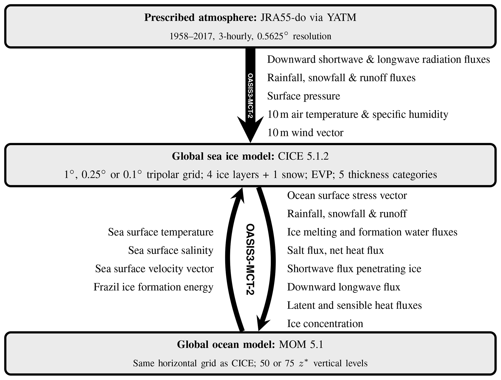
Figure 1ACCESS-OM2 model components and coupling fields. OASIS3-MCT-2 is used to couple the model components. Notice that MOM 5.1 receives atmospheric forcing via CICE 5.1.2 rather than directly from YATM (CICE 5.1.2 is configured with the same global domain and horizontal grid as MOM 5.1). Surface pressure is passed from CICE 5.1.2 to MOM 5.1 but is not used by MOM 5.1 in the current configuration so is not shown. Similarly, the sea surface slope vector is passed from MOM 5.1 to CICE 5.1.2 but is unused (the sea surface slope is instead calculated from the sea surface velocity vector, assuming geostrophy).
2.1 MOM5 ocean model
MOM5 is a hydrostatic primitive equation ocean model with a free surface discretized using the Arakawa B grid for the horizontal stencil along with a variety of vertical coordinate options (Griffies, 2012). We make use of the Boussinesq (volume-conserving) version of the code and choose the z* vertical coordinate. The model is derived from a long history of use in climate and ocean modelling (documented in an unpublished manuscript available from https://mom-ocean.github.io/assets/pdfs/mom_history_2017.09.19.pdf, last access: 21 January 2020) and is comprehensively documented (Griffies, 2012); in this paper we therefore focus on detailing aspects of the MOM configuration that are specific to ACCESS-OM2.
2.1.1 Vertical grid
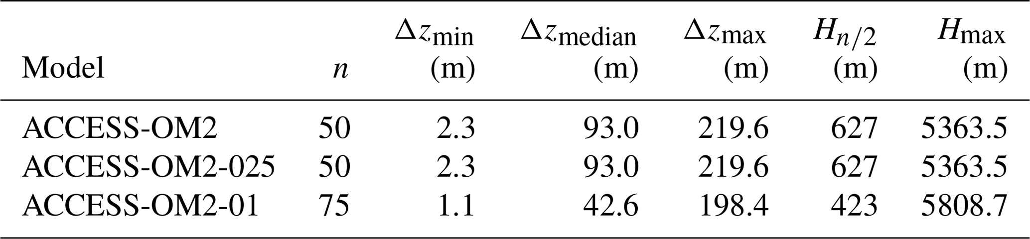
The configurations use a z* vertical coordinate (Stacey et al., 1995; Adcroft and Campin, 2004) with partial cells (Adcroft et al., 1997; Pacanowski and Gnanadesikan, 1998). The vertical grids are optimized for resolving baroclinic modes based on the KDS grids recommended by Stewart et al. (2017), who suggest that finer horizontal resolution necessitates finer vertical resolution. The vertical grids in ACCESS-OM2 and ACCESS-OM2-025 are slightly modified versions of KDS50, with 50 levels and 2.3 m spacing at the surface, increasing smoothly to 219.6 m by the bottom at 5363.5 m. The vertical grid in ACCESS-OM2-01 is a slightly modified version of KDS75, with 75 levels and 1.1 m spacing at the surface, increasing smoothly to 198.4 m by the bottom at 5808.7 m. Since we refine both vertical and horizontal resolution in ACCESS-OM2-01, we cannot distinguish their effects in our results. Details of the vertical discretization can be found in Table 1.
Table 1Vertical grid parameters: n levels, with spacing of Δzmin and Δzmax at the surface and maximum depth Hmax, respectively, and median spacing Δzmedian. The depth at level n∕2 is denoted Hn∕2.
2.1.2 Horizontal grid
In the horizontal direction, MOM5 and CICE5 both use the same orthogonal curvilinear Arakawa B grid with velocity components co-located at the northeast corner of tracer cells. Model configurations have been developed with zonal grid spacings of 1, 0.25, and 0.1∘ south of 65∘ N. Globally, the median zonal cell size is 92, 18.1, and 7.2 km, respectively, at 1, 0.25, and 0.1∘ resolution. Although the CICE model is global, the sea ice is mostly confined to latitudes poleward of 60∘, where the median of the largest dimension of ocean cells is 49.1, 11.7, and 4.7 km, respectively, at the three resolutions.
The horizontal meshes are 360×300, 1440×1080, and 3600×2700 at 1, 0.25, and 0.1∘, respectively (see Table 2). Ocean cells cover the global ocean from the North Pole to the Antarctic ice shelf edge (77.9∘ S at 1∘; 78.2∘ S at 0.25∘; 79.6∘ S at 0.1∘). The longitude range is −280 to +80∘ E, placing the join in the middle of the Indian Ocean. The grid is tripolar (Murray, 1996) in all configurations, with two northern poles placed on land at 65∘ N, −100∘ E and 65∘ N, 80∘ E, and a third pole at the South Pole; consequently, the grid directions are zonal and meridional only south of 65∘ N. In the 0.25 and 0.1∘ configurations the grid is Mercator (i.e. the meridional spacing scales as the cosine of latitude) between 65∘ N and 65∘ S; south of 65∘ S, the meridional grid spacing is held at the same value as at 65∘ S. The meridional variation of meridional grid spacing is more complicated in the 1∘ model and incorporates a refinement to 1/3∘ within 10∘ of the Equator (Bi et al., 2013b).
2.1.3 Bathymetry
The model bathymetry for ACCESS-OM2 makes use of legacy datasets from ACCESS-OM at 1∘ resolution (Bi et al., 2013b). ACCESS-OM2-025 uses a modified version of the GFDL-CM2.5 bathymetry as used by Griffies et al. (2005). Significant effort was deployed to create a new model bathymetry file for ACCESS-OM2-01 based on version 20150318a of the GEBCO 2014 30 arcsec grid (GEBCO, 2014). To obtain the depth of each model cell a simple mean of points with depth greater than zero within the cell was calculated along with the fraction of such wet points. After the elimination of isolated lakes, the coasts were inspected by eye and hand-edited to ensure major straits and channels (e.g. Lombok Strait) could be represented by the B grid, small shallow inlets were removed, and global connectivity was maintained. Further checks were also made to eliminate non-advective cells and to ensure that the averaging process did not remove significant islands or smooth subsurface features too aggressively (e.g. Macquarie Island). In regions where ice shelves are found, topography ends at a vertical wall at the ice shelf edge (the calving line, not the grounding line); there are no ice shelf cavities as these are not supported in MOM5. The coarser two resolutions expanded the land mask to remove small wet cells close to the northern tripoles, but the ACCESS-OM2-01 bathymetry retains these cells and therefore includes the Gulf of Ob in Siberia and many additional channels in the Canadian Archipelago. These bathymetric and land mask inconsistencies may contribute to the differences in model behaviour at different resolutions. We use partial cells (Adcroft et al., 1997; Pacanowski and Gnanadesikan, 1998) to obtain a more accurate representation of bottom topography in all three configurations. In ACCESS-OM2 and ACCESS-OM2-025 the minimum thickness of partial cells is 20 % of the full cell thickness Δz. In ACCESS-OM2-01 the minimum thickness of partial cells is 0.2Δz, or , whichever is greater. The minimum water depth is 45.11 m (10 levels) in ACCESS-OM2, 40.36 m (9 levels) in ACCESS-OM2-025, and 10.43 m (7 levels) in ACCESS-OM2-01.
2.1.4 Parameterizations and equation of state
A sub-grid-scale parameterization for mesoscale eddies is included in the ACCESS-OM2 and ACCESS-OM2-025 models but not in ACCESS-OM2-01 as this resolution is considered eddy-resolving. In the two coarser configurations the Gent and McWilliams (1990) (GM) parameterization is used to represent the quasi-Stokes transport associated with mesoscale eddies (McDougall and McIntosh, 2001), and the neutral-direction diffusive tracer transport is parameterized by a neutral diffusivity (Redi, 1982). The GM parameterization is implemented as a skew-diffusive flux (Griffies, 1998) and further formulated as a boundary value problem by Ferrari et al. (2010). The associated diffusivity is depth-independent but flow-dependent and is the product of an inverse timescale, a squared length scale, and a grid scaling factor as detailed in Sect. 3.3 of Griffies et al. (2005). The length scale is 50 km at 1∘ and 20 km at 0.25∘. The inverse timescale is an Eady growth rate determined from the horizontal density gradient averaged between 100 and 2000 m using a constant buoyancy frequency of 0.004 s−1 (these three values are the defaults). The Eady growth rate is subject to a limiter and is smoothed both vertically and horizontally, and it is vertically averaged in the mixed layer. The GM diffusivity is also scaled in proportion to how well the numerical grid resolves the first baroclinic Rossby radius (or the equatorial Rossby radius within ±5∘ latitude), as suggested by Hallberg (2013). The GM diffusivity is limited to the ranges 50–600 m2 s−1 in ACCESS-OM2 and 1–200 m2 s−1 in ACCESS-OM2-025.
The neutral tracer diffusion is implemented according to Griffies et al. (1998) and is used in the two coarser configurations with a diffusivity that differs from GM. A constant coefficient of 600 m2 s−1 is used in ACCESS-OM2, while in ACCESS-OM2-025 the coefficient is scaled by the resolution of the grid relative to the first baroclinic Rossby radius (or the equatorial Rossby radius within ±5∘ N latitude) with a diffusivity no greater than 200 m2 s−1.
All three configurations include a parameterization for re-stratification in the surface mixed layer due to submesoscale eddies (Fox-Kemper et al., 2008). This parameterization applies an overturning circulation dependent on the horizontal buoyancy gradients within the mixed layer. The optional horizontal diffusive portion of this parameterization is not used.
Horizontal friction is implemented with a biharmonic operator and a horizontally isotropic Smagorinsky scaling for the viscosity coefficient (Griffies and Hallberg, 2000; Griffies, 2012). The ACCESS-OM2 configuration also has a grid-spacing-dependent horizontally isotropic biharmonic background viscosity set by a velocity scale 0.04 m s−1, with the NCAR scheme applied to enhance the background horizontal viscosity near western boundaries in order to ensure the western boundary currents are resolved (see Sect. 3.4 of Griffies et al., 2005). ACCESS-OM2 also uses a Laplacian bottom viscosity set by a velocity scale 0.01 m s−1. There is no background viscosity at the other resolutions. The overall biharmonic viscosity is limited to 25 % of the numerical instability threshold in ACCESS-OM2 or 100 % in the other two configurations. The biharmonic viscosity varies in space and time; at the surface in western boundary currents it is of order 1014, 1012, and 1010 m4 s−1 in ACCESS-OM2, ACCESS-OM2-025, and ACCESS-OM2-01 (respectively), corresponding to viscous western boundary current widths (Haidvogel et al., 1992) of about 350, 100, and 60 km (respectively), which are well-resolved by the grid in all cases. The lateral boundary condition for velocity is no-slip, which is the only boundary condition supported by MOM5 on a B grid (Griffies, 2012).
A constant background vertical viscosity of 10−4 m2 s−1 is used at all resolutions. The background vertical tracer diffusivity is zero in ACCESS-OM2-025 and ACCESS-OM2-01, but at 1∘ it is dependent on latitude following Jochum (2009), smoothly increasing from m2 s−1 at the Equator to a constant m2 s−1 poleward of ±20∘ N. The K-profile parameterization (KPP; Large et al., 1994) determines additional vertical diffusivities of both tracers and momentum to represent mixing within the surface boundary layer and also Richardson-number-based shear instability (active mainly in the equatorial undercurrents), internal wave breaking, and double diffusion in the interior. KPP maintains static stability by applying large vertical diffusivity in regions with a small or negative Richardson number, removing the need for explicit convective adjustment. There are no explicit tides, but bottom-enhanced internal tidal mixing is parameterized following Simmons et al. (2004) and barotropic tidal mixing is parameterized following Lee et al. (2006). We calculate bottom drag from the law of the wall using prescribed bottom roughness and spatially resolved but temporally constant tidal current speed, with residual 0.05 m s−1. Overflow and down-slope mixing schemes are not used in ACCESS-OM2-025 or ACCESS-OM2-01, but in ACCESS-OM2 we use sigma transport (Beckmann and Döscher, 1997; Campin and Goosse, 1999; Döscher and Beckmann, 2000) with default parameters and down-slope mixing.
At 1∘ Rayleigh damping is used to improve the Indonesian throughflow transport; a damping timescale of 1.5 h is applied at all but the bottom two (three) U cells in Lombok (Ombai) Strait and for 3 ∕ 4 of the width of the Torres Strait at all depths. At 0.1∘ a damping timescale of 1.5 h is used at all depths across the full width of Kara Strait to constrain the velocity, which otherwise leads to numerical instability unless an unfeasibly small time step is used. There is no Rayleigh drag in the 0.25∘ configuration.
We use the Jackett et al. (2006) pre-TEOS10 seawater equation of state and freezing temperature. The prognostic temperature variable is conservative temperature in the 1 and 0.25∘ configurations and potential temperature at 0.1∘. All configurations use practical salinity as the prognostic variable for salt.
2.1.5 Numerical methods
All configurations use a baroclinic dynamics (and tracer) time step that is 80 times longer than the barotropic time step. The barotropic dynamics use a predictor–corrector method with dissipation parameter γ=0.2 and Laplacian smoothing of sea surface height. The baroclinic time stepping uses a two-level volume- and tracer-conserving staggered second-order forward method, with implicit vertical mixing and semi-implicit Coriolis calculations. Momentum advection is achieved via a second-order centred operator in space and third-order Adams–Bashforth time stepping. We use a multidimensional piecewise parabolic scheme for tracer advection (Colella and Woodward, 1984), with a monotonicity-preserving flux limiter following Suresh and Huynh (1997).
2.2 CICE5 sea ice model
CICE5 is a thermodynamic–dynamic sea ice model, including advective transport of the state variables and an energy-conserving ridging parameterization that transfers ice between thickness categories in response to the energy budget and strain rates. The CICE5 sea ice model is well-documented (Hunke et al., 2015), so we only provide an overview of key aspects here. We use CICE version 5.1.2 with parameters that are largely based on those used for CICE4.1 in ACCESS-OM (Bi et al., 2013b). In our configuration CICE5 uses the same horizontal tripolar Arakawa B grid as MOM5, and its thermodynamic time step is the same as the MOM5 baroclinic time step (Table 2). For the thermodynamics we use four ice layers and one snow layer for each of the five thickness categories (discussed below). We use the Bitz and Lipscomb (1999) thermodynamics formulation at 1 and 0.25∘, but at 0.1∘ this occasionally failed to converge so the mushy ice thermodynamics formulation of Turner et al. (2013) was used instead in the highest-resolution simulation. Other thermodynamic parameters are the same as those listed in Bi et al. (2013b, Table 2) for ACCESS-OM, including the use of the Pringle et al. (2007) thermal conductivity parameterization, which improves the otherwise slow thermodynamic ice growth rate in the Antarctic (Hunke, 2010).
Horizontal advection of conserved properties is handled by the incremental remapping scheme of Dukowicz and Baumgardner (2000) and Lipscomb and Hunke (2004). Internal ice stresses are represented by a visco-plastic rheology via the “classic” elasto-visco-plastic (EVP) method (Hunke and Dukowicz, 1997, 2002; Hunke, 2001) in which a fictitious elastic term is added to facilitate efficient numerical convergence to the Hibler (1979) visco-plastic solution via damped elastic waves, which are supposed to decay to negligible amplitude via elastic sub-time steps within each dynamic time step. For pragmatic reasons we follow Hunke and Dukowicz (2002) in using 120 elastic time steps per dynamic time step, but we note that this may be insufficient to completely eliminate the elastic transients from the solution (Losch and Danilov, 2012; Lemieux et al., 2012; Kimmritz et al., 2017, 2015). The ice dynamics have the same time step as the thermodynamics at the two coarser resolutions, but at 0.1∘ it was necessary to reduce the dynamic time step to a third of the thermodynamic time step due to a more restrictive CFL condition because the land mask edge is closer to the northern poles in our tripolar grid, producing some very small grid cells. The resulting load imbalance was mitigated by allocating relatively more cores to CICE at 0.1∘ (Table 2).
In all three configurations the vertical grid resolution is sufficient to resolve the surface Ekman layer (Table 1), so we use a turning angle of zero, consistent with ACCESS-OM (Bi et al., 2013b, Table 2). We use an ice–ocean drag coefficient of 0.00536, consistent with ACCESS-OM (Bi et al., 2013b, Table 2) and very close to the value of 0.0054 measured at 0.5 m below first-year landfast ice by Shirasawa and Ingram (1997).
Importantly, every model grid cell may contain a mixture of open water and sea ice, with the ice itself being split into a number of thickness categories chosen to represent the inhomogeneous thickness distribution of sea ice. We use five thickness categories, with lower bounds of 0, 0.64, 1.39, 2.47, and 4.57 m. Following Thorndike et al. (1975) ice mass is moved between these categories as a function of ice motion and advection, the thermodynamic ice growth rate, and the ridging redistribution. We use the Lipscomb et al. (2007) ridging scheme, with the e-folding scale parameter taking the default value 3 m1∕2 (rather than 2 m1∕2 as used in ACCESS-OM Bi et al., 2013b, Table 2).
The CICE5 configurations of the final runs reported here subdivided the computational domain horizontally into tiles, with around four (six) tiles allocated to each CPU at 0.25∘ (0.1∘) by a roundrobin distribution (Craig et al., 2015), which omits land-only tiles and improves the load balance by having a mix of ice-containing and ice-free tiles allocated to each CPU.
At 1∘ we allocate one pole-to-pole meridional strip to each processor in the interest of load balancing.
We also use halo masking at all resolutions, which eliminates message passing updates in ice-free halos.
2.3 Forcing
The ACCESS-OM2 configurations are forced with the JRA55-do v1.3 atmospheric product (Tsujino et al., 2018), which has improved spatial and temporal resolution (55 km, 3-hourly) and temporal extent (1958–2018) compared to the Large and Yeager (2009) CORE-II dataset (200 km, 6-hourly, 1948–2009) used in many previous modelling studies. JRA55-do is more dynamically self-consistent than CORE-II and has smaller biases in surface wind and temperature (Figs. 12, 28, 29, 42, 43, 46, 47 in Tsujino et al., 2018) but a larger bias in specific humidity (Figs. 44, 45 in Tsujino et al., 2018). The improved spatial resolution of wind is important for a better representation of coastal polynyas (Stössel et al., 2011; Zhang et al., 2015) and upwelling (Taboada et al., 2019). JRA55-do has more realistic Greenland runoff (an order of magnitude larger than in CORE-II) and includes recent Antarctic calving and basal melt estimates from Depoorter et al. (2013), which are spatially variable and somewhat larger than the uniform values in CORE-II (Tsujino et al., 2018). The temporal coverage currently extends from 1 January 1958 to 1 February 2018, but it is regularly updated to near present day; we use 1958–2017 inclusive for the experiments described in this paper. JRA55-do v1.3 provides 3-hourly liquid and solid precipitation, downward surface longwave and shortwave radiation, sea level pressure, 10 m wind velocity components, 10 m specific humidity, and 10 m air temperature on a TL319 grid (0.5625∘ resolution). JRA55-do also provides total runoff (river, calving, and basal melt) at 0.25∘ resolution; river runoff is daily and interannually varying (Suzuki et al., 2018), Greenland runoff is monthly climatological (Bamber et al., 2012), and Antarctic calving and basal melt are climatological means (Depoorter et al., 2013). Liquid runoff is deposited at the coast in the top 40 m of the ocean, whereas solid runoff and basal melt are deposited as liquid at the ice shelf edge at the surface. The total runoff is spread horizontally if needed to keep the flux below a threshold (see Sect. 2.3.1).
Surface forcing is handled globally by CICE5, which then passes various forcing fluxes on to MOM5 (Fig. 1). We use Large and Yeager (2004) turbulent flux bulk formulas to calculate the air–ocean drag coefficient, evaporative transfer coefficient, and sensible heat transfer coefficient. The calculation uses the air–ocean velocity difference with an additional component to account for gustiness. Note that the implementation differs from Large and Yeager (2004) in having a 0.5 m s−1 floor for the 10 m relative wind speed and a ceiling of 10 for the absolute value of the stability parameter ζ. We used two Monin–Obukhov iterations, which Large and Yeager (2004) state is appropriate over the ocean but less than their suggested value of 5 over sea ice. In calculating the wind stress on the ocean we use the wind velocity relative to the ocean surface velocity, whereas we use the absolute wind velocity to calculate wind stress on sea ice. Wind velocity in JRA55-do has been adjusted to match time-mean scatterometer and radiometer winds, which are relative to the ocean surface current; Tsujino et al. (2018) recommend adding a climatological mean surface current to JRA55-do winds to better represent absolute winds, but this suggestion has not been tested in an ocean model and so we did not take that approach here. We also note that the lack of coupled negative feedback with a dynamic atmosphere may produce (for example) overly large heat and momentum fluxes in response to the imposed JRA55-do forcing fields (Hyder et al., 2018; Renault et al., 2016).
Ocean albedo has the constant value 0.1, which is larger than the value 0.06 used in ACCESS-OM (Bi et al., 2013b). In CICE5 we use the same NCAR CCSM3 shortwave distribution method, ice and snow albedos in the visible and infrared bands, and melt albedo parameters as in ACCESS-OM (Bi et al., 2013b, their Table 2), but we use the default snow patchiness parameter 0.02 m instead of the value 0.01 m used in ACCESS-OM. Shortwave penetration into the ocean is handled by the GFDL scheme, with Manizza et al. (2005) optics using a prescribed monthly chlorophyll a climatology as used in GFDL's CM2.5 and CM2.6 (Delworth et al., 2012; Griffies et al., 2015) based on SeaWiFS data for 1998–2006 and the method of Sweeney et al. (2005). There is no representation of geothermal heating.
We restore sea surface salinity (SSS) to the interpolated 0.25∘ World Ocean Atlas 2013 v2 monthly climatology (WOA13, also used for initial conditions; see Sect. 2.4), with a spatially constant offset to ensure that the net restoring salt flux is zero for each time step. Restoring is applied globally (including under ice) via a salt flux, with a timescale set by the “piston velocity” (surface vertical grid spacing divided by restoring timescale) of 33 m per 300 d in all cases. The SSS restoring flux is determined from the difference between the model and WOA13 SSS; the restoring flux is calculated from the maximum of this difference or ±0.5 psu in order to avoid excessively large fluxes. We impose a constraint of zero net water flux into the ocean from the coupler by removing the area mean of precipitation P minus evaporation E plus runoff R from P−E so that the integrated is zero at each time step; this does not constrain water exchanges between the ocean and sea ice. These restoring and water flux choices are typical of CORE-II models (Danabasoglu et al., 2014, Table 2).
The model sea ice has a fixed bulk salinity (5 g kg−1). This salt is obtained from the seawater when sea ice is formed; this can drive ocean salinity below zero in regions fresher than the ice salinity, for example during the spring melt in the shallow Siberian gulfs that are resolved in the ACCESS-OM2-01 model bathymetry. This problem was resolved in ACCESS-OM2-01 by setting the local ocean–ice salt flux to zero in regions where the seawater salinity is less than 6 g kg−1; in these regions the sea ice salt is instead obtained from the global surface ocean to ensure the conservation of salt in the ice–ocean system. Over a sea ice formation and melt cycle this produces a small unphysical transport of salt from the global surface ocean to regions where such sea ice melts.
2.3.1 YATM and libaccessom2
ACCESS-OM2 uses a new atmospheric driver, known as YATM, that implements a file-based atmosphere and replaces MATM, which was used in ACCESS-OM (Bi et al., 2013b). Its purpose is to track model time and, when necessary, read the appropriate forcing fields from files and deliver them to the coupler. This is implemented via an associated library (libaccessom2; https://github.com/COSIMA/libaccessom2, last access: 21 January 2020) that is linked into YATM, CICE, and MOM to provide shared functionality and an interface to inter-model communication and synchronization tasks.
YATM is also responsible for remapping river runoff in real time. This is done separately from the other forcing fields because it is difficult to do in a distributed memory setting, since ensuring runoff is on coastal points may require interprocess communication. Remapping is done in two steps: first runoff is moved to the destination grid using conservative interpolation, and then it is distributed from land to coastal points using an efficient nearest-neighbour algorithm based on a pre-computed k-dimensional tree (k-d tree) data structure (Bentley, 1975). We use the KDTREE2 Fortran k-d tree implementation (https://github.com/jmhodges/kdtree2, last access: 21 January 2020). The k-d tree is also used to conservatively spread runoff into the neighbouring ocean grid points to ensure it does not exceed a prescribed cap. ACCESS-OM2 and ACCESS-OM2-025 use a runoff cap of 0.03 kg m−2s−1 globally. In ACCESS-OM2-01 there are reduced caps of 0.001 and 0.003 kg m−2 s−1 at the mouths of some Arctic rivers to produce broader spreading and avoid excessively low salinity and a cap of 0.03 kg m−2 s−1 everywhere else.
2.4 Initial conditions
The experiments discussed in Sect. 4 ran for different lengths of time (Fig. 3). The ACCESS-OM2 and ACCESS-OM2-025 experiments were run for five 60-year cycles (1 January 1958–31 December 2017) of JRA55-do. The ocean was initially at rest, with zero sea level and with temperature and salinity from the World Ocean Atlas 2013 v2 (Locarnini et al., 2013; Zweng et al., 2013) 0.25∘ “decav” product (the average of six decadal averages spanning 1955–2012). The initial sea ice concentration and thickness are 100 % and about 2.5 m (respectively) in regions north of 70∘ N and south of 60∘ S where the sea surface temperature is less than 1 ∘C above freezing, with a parabolic distribution of area across the five ice thickness categories. The initial snow thickness in each category is 0.2 m or 20 % of the ice thickness in that category, whichever is smaller. The total sea ice and snow volumes in this initial condition are very close to the adjusted state; there is therefore no significant drift in total ocean salt as the sea ice spins up.
The ACCESS-OM2-01 experiment ran for 33 years from 1 January 1985–31 December 2017. It was started from a 40-year spin-up under repeated 1 May 1984–30 April 1985 JRA55-do forcing, which we term repeat-year forcing (RYF). This 12-month RYF period was chosen because it is particularly neutral in terms of the major modes of climate variability (Stewart et al., 2020). This spin-up began from the same initial condition as the ACCESS-OM2 and ACCESS-OM2-025 runs. The RYF spin-up contained some parameter changes, in particular the ice–ocean stress turning angle was changed from 16.26∘ to zero at the start of August in the 12th year. Before this change the Arctic ice volume built up significantly (and unrealistically) in the thickest category, but it began a slow decline when the turning angle was set to zero, which persisted into the first ∼6 years of the interannually forced run (Fig. 27c). The 1984–1985 repeat-year forcing contained some biases relative to climatology; for example, biases in the North Pacific wind stress curl produced a northward bias in the separation of the Kuroshio Current in the ACCESS-OM2-01 initial condition (i.e. the end of the RYF spin-up), which largely disappeared under the subsequent interannually varying forcing (Fig. 21).
2.5 Coupling
Figure 1 shows the fields that are transferred between the model components. The prescribed atmosphere drives the global ice model, which is two-way coupled to the ocean model. Coupling is implemented using the Ocean Atmosphere Sea Ice Soil (OASIS3-MCT; Valcke et al., 2013) coupler version 2.0, developed at CERFACS and CNRS, France (https://portal.enes.org/oasis, last access: 21 January 2020). The coupling strategy is based on the ACCESS-OM model (Bi and Marsland, 2010) but uses a newer library-based version of OASIS which is capable of parallel coupling. The atmosphere-to-CICE5 coupling time step is determined by the frequency of the atmospheric forcing dataset (i.e. 3-hourly for JRA55-do). Two-way CICE5-MOM5 coupling takes place at every time step (i.e. every ocean baroclinic time step and ice thermodynamic time step). In order to avoid coupled ice–ocean instabilities (Hallberg, 2014), MOM5 is configured to neglect the weight of sea ice when determining the sea surface height.
No grid remapping is needed between CICE and MOM because they use identical grids, but the atmospheric forcing requires remapping onto the CICE grid. The default remapping method used within OASIS3-MCT (SCRIP; https://github.com/SCRIP-Project/SCRIP, last access: 21 January 2020) does not scale to 0.1∘ grid spacing for global models. Instead the grid remapping interpolation weights are calculated using the RegridWeightGen application, which is part of the Earth System Modeling Framework (https://www.earthsystemcog.org/projects/esmf/, last access: 21 January 2020). Fluxes are remapped using conservative interpolation (second-order for ACCESS-OM2 and ACCESS-OM2-025, first-order for ACCESS-OM2-01). Non-flux fields do not need conservative remapping, so we use patch recovery (Kritsikis et al., 2017; Khoei and Gharehbaghi, 2007) to produce very smooth destination fields; this is particularly important for the ACCESS-OM2-025 and ACCESS-OM2-01 configurations because they have finer resolution than the forcing dataset.
The computational performance of a coupled model depends upon the runtimes of each of its component models, the coupler overhead, and any potential load imbalances between each component. The computational load of ACCESS-OM2 is dominated by MOM5, which typically comprises around 90 % of CPU time at the lower resolutions and 75 % of this time at 0.1∘ resolution. The remainder of CPU time is predominantly due to CICE5, with a negligible contribution from the coupling and the YATM file-based atmospheric model. Despite playing a smaller computational role, CICE5 can limit the overall scalability and performance of the coupled ocean–sea ice model because its runtime depends on sea-ice-covered area, which changes seasonally and causes load imbalances that are exacerbated at higher resolutions and core counts.
Here we report measurements of the runtime of the MOM5 and CICE5 model components as a function of resolution and core count. In all cases the initial condition was taken from spun-up runs on 1 January (in 2003 in the fifth cycle at 1∘, 2000 in the fifth cycle at 0.25∘, and 2000 at 0.1∘; see Sect. 4). All simulations were performed on Raijin, the peak machine at Australia's National Computation Infrastructure. For the test runs, executables were compiled with Intel compiler suite 2019 and OpenMPI 3.0.3. Runtimes were measured on a 3592-node platform, on which each node includes two Xeon Sandy Bridge (E5-2670) CPUs of speeds 2.6 GHz (base) to 3.0 GHz (turbo), with a total of 16 cores per node, and 32 GB of external DDR3-1600 RAM. Nodes are connected by an InfiniBand FDR-14 interconnect, with peak transfer speeds of 56 Gb s−1. Model data are stored on a Lustre parallel file system. On this platform, MOM5 and CICE5 computation is observed to be predominantly memory-bound, with computational performance limited by DRAM bandwidth and on the order of 1 GFLOP s−1 per CPU, although the heterogeneity of the various model solvers will exhibit different degrees of performance throughout the codes. In general, performance will improve as the number of CPUs is increased, and there will be a transition from a memory-bound to a communication-bound state as the data transfer costs exceed RAM speeds.
We first present measurements of MOM5 and CICE5 runtime scalability with respect to computational core count and consider performance over several CPU configurations. The performance of the coupled ocean–sea ice model is inferred from the independent performance of CICE5 and MOM5, leading to recommended standard configurations.
3.1 MOM5 scalability
We conduct a series of tests on the scalability of MOM5 at each of the three model resolutions tested here, configured as described in Sect. 2.1. The tests used baroclinic time steps of 5400, 1800, and 400 s at 1, 0.25, and 0.1∘ (respectively). In each test we record the main loop runtime per baroclinic time step for three short simulations at a prescribed core count and repeat this test for different core counts. The length of each simulation in model time is set to ensure a runtime of approximately 3 min and varies from 2 months at the lowest resolution to 1 d at the highest resolution. We report the runtime per model time step (Fig. 2a) and the total CPU time (Fig. 2b) for each configuration. Each point denotes the average runtime over all MPI ranks for each run. Note that the numbers provided here do not include start-up time or any infrequent I/O events, typically on monthly or annual timescales, which can add considerable cost, especially at high core counts.
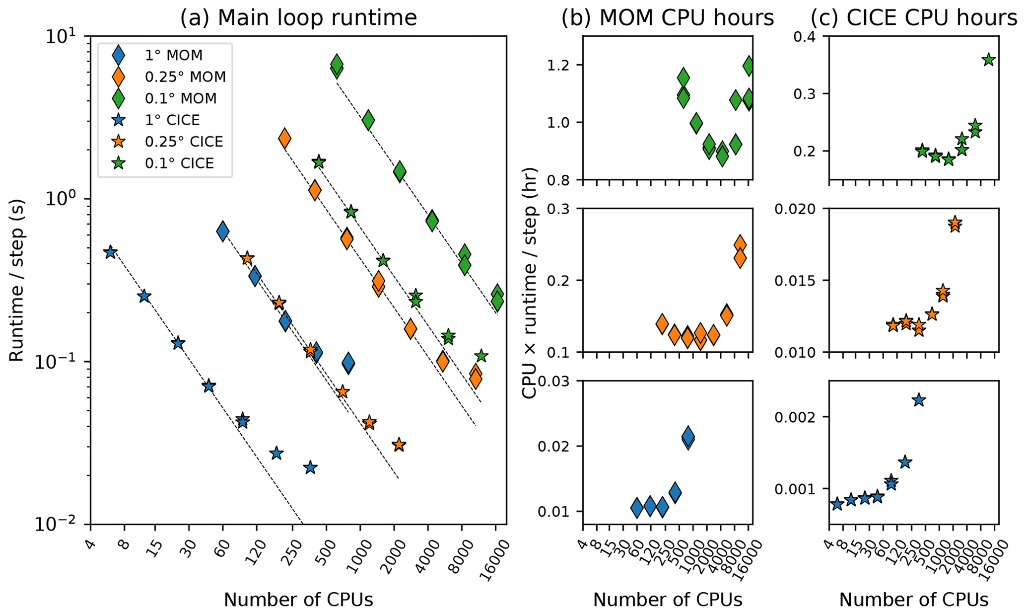
Figure 2Scaling performance for MOM5 and CICE5 global model simulations showing (a) runtime per ocean baroclinic time step, (b) CPU time per ocean baroclinic time step, and (c) CPU time per ice thermodynamic time step as a function of the number of processors for a short simulation at each model resolution. The dashed lines in panel (a) indicate perfect linear scaling.
These tests demonstrate the highly efficient scalability of MOM5. For the standard (1∘ grid spacing) ACCESS-OM2 configuration, the model scales well to core counts of 400 and only begins to degrade at 800 cores. At 400 cores, one model year takes just 10 min (equivalent to a theoretical maximum of 144 model years per day). While higher resolutions require considerably more computational time, MOM5 still scales outstandingly well – to over 2800 cores for ACCESS-OM2-025 (achieving 46 min per model year, i.e. over 30 model years per day) and up to 16 000 cores for ACCESS-OM2-01 – and runtimes can often be sustained when provided with a sufficient number of CPUs. This demonstrates efficient scaling well beyond the 512 cores investigated by Schmidt (2007). On our platform, a MOM5 configuration of 0.1∘ grid spacing could achieve a maximum theoretical performance of almost 5 years per day, although start-up and model I/O would reduce the speed in any practical case.
These results highlight the scaling efficiency of MOM5 and give us flexibility to choose different MOM5 core counts for different configurations. However, the behaviour of the coupled ocean–sea ice model is also dependent on CICE5 performance, as discussed below.
3.2 CICE5 scalability
Analogous scaling tests for CICE5 were also undertaken, configured as described in Sect. 2.2, except that the distribution scheme was sectrobin rather than roundrobin (Craig et al., 2015) at 0.25 and 0.1∘ (with four tiles per core at 0.1∘), and at 1∘ an ice–ocean stress turning angle of 16.26∘ was used (instead of zero).
The tests used thermodynamic time steps of 5400, 1800, and 400 s at 1, 0.25, and 0.1∘ (respectively).
These tests show that at 1∘ grid spacing the model scales up to ∼50 cores, up to 500 cores at 0.25∘, and 2000 cores at 0.1∘ (Fig. 2a, c).
Even at higher than optimal core counts, scaling is acceptable.
However, these numbers obscure some more complex issues. First, the effective performance of CICE5 is variable, partly because ice cover is seasonal, so different tiles have a different amount of work to do at different times of year. This variability is mitigated by the distribution scheme, which assigns multiple tiles from different regions to be computed on each core. While the code itself scales well with the number of cores, the total amount of work required increases more rapidly in CICE5 at higher resolutions. That is, the additional CPU time required for each MOM5 model time step increases by a factor of 90 in going from 1 to 0.1∘ grid spacing (Fig. 2b), whereas for CICE5 the CPU time required per time step increases by a factor of 200, with a disproportionately large increase between 0.25 and 0.1∘ (Fig. 2c). We mainly attribute this to changing from one to three dynamic time steps per thermodynamic time step between 0.25 and 0.1∘, exacerbated by using the slower mushy thermodynamics, but residual load imbalances may also contribute. Consequently, we use relatively more cores for CICE5 than for MOM5 at higher resolution – the ratio of ice to ocean cores is 0.11 in ACCESS-OM2, 0.25 in ACCESS-OM2-025, and 0.35 in ACCESS-OM2-01 (Table 2).
3.3 Coupled ocean–sea ice model configuration
The performance of the coupled ocean–sea ice model is limited by the scaling performance and resource requirements of both components, as well as their load balancing and variability. This load balance is further complicated by the differing performance of components as a function of resolution and by the need to alter the model time step for some simulations. It is clear from Fig. 2a that balancing the runtime of the model components requires more cores for MOM5 than CICE5, but the ratio depends on resolution. Since CICE5 has a lower core count than MOM5 at all resolutions, if imbalances are to exist, we aim to ensure that CICE5 is waiting for MOM5. The standard configurations, core counts, and typical performance of differing model resolutions are shown in Table 2.
Table 2Outline of model grid, size, cores, and typical performance for production runs. The time step given is the ocean baroclinic time step (at 0.1∘ this differs from the 400 s time step used in the scaling tests), which equals the ice thermodynamic time step (but is 3 times longer than the ice dynamic time step at 0.1∘). Configuration improvements subsequent to the runs shown here have halved the ACCESS-OM2-01 wall time and CPU hour cost.
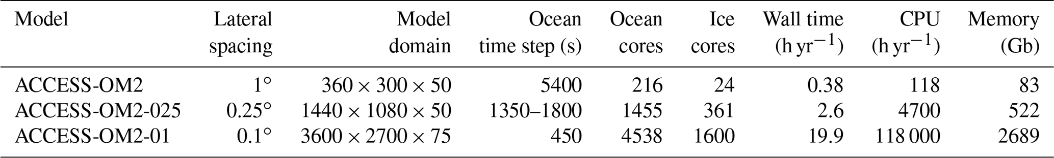
The configurations shown here are under continuous development and optimization, and it is anticipated that improvements in model stability and load balancing will continue to improve performance in the future (for example, we have recently doubled ACCESS-OM2-01 performance relative to the figures in Table 2). We have also configured a minimal ACCESS-OM2-01 configuration with a total core count of ∼2000 to aid in testing and to run on smaller systems. These configurations will be continually released and documented on the ACCESS-OM2 code repository as they are developed.
We now outline results from ACCESS-OM2 using simulations with each of the three horizontal resolutions outlined in Table 2. Each of the three simulations is forced by the interannual JRA55-do forcing dataset (Tsujino et al., 2018), which currently covers 60 years from 1958 until the end of 2017. The lower-resolution simulations (both ACCESS-OM2 and ACCESS-OM2-025) continuously cycle through five iterations of this dataset, giving a 300-year simulation, following the CORE-II protocol (e.g. Danabasoglu et al., 2014) and the CMIP6/OMIP protocol (Griffies et al., 2016). Selected global diagnostics from these simulations are shown by the blue and orange lines (respectively) in Fig. 3, where dates have been aligned so that the last cycle of forcing matches the calendar dates of the forcing dataset (giving a nominal start year of 1718). The main period of model evaluation will be the final interannual forcing cycle, the years 1958–2017 inclusive. When time-averaged fields are shown, averages are taken over the last 25 years of simulation (the years 1993–2017 inclusive) unless stated otherwise.

Figure 3Time series of the global average of annual mean (a) ocean temperature, (b) sea surface temperature, (c) sea surface salinity, and (d) ocean kinetic energy for each of the simulations. Output is shown for the full interannually forced model simulations, including five interannual forcing cycles for ACCESS-OM2 and ACCESS-OM2-025, with the timescale compressed for the first four cycles and the end of each forcing cycle indicated by a vertical line. The dashed black curve in (b) is the observed sea surface temperature anomaly (ERSST v4; Huang et al., 2019) offset by 18 ∘C to compare the rate of warming over the final cycle of forcing. Model time has been offset to ensure that the final cycle has a date that is consistent with the forcing date, allowing the short, 33-year ACCESS-OM2-01 simulation to be plotted on the same time axis.
The highest-resolution simulation, using ACCESS-OM2-01, is ∼1000 times more computationally intensive than ACCESS-OM2 and ∼25 times more computationally intensive than ACCESS-OM2-025 (see Table 2). A full simulation with five interannual forcing cycles of ACCESS-OM2-01 is not possible with current computing resources, and hence we use an alternative spin-up strategy. As discussed in Sect. 2.4, in this case we select a repeat-year forcing (RYF) spin-up strategy (Stewart et al., 2020), in which the time period 1 May 1984–30 April 1985 is repeated continuously. This spin-up has been run for 40 years, after which we conduct an interannually forced simulation from 1985 through 2017. It is this interannual simulation period which is used for the model evaluation in this paper, as indicated by the green line in Fig. 3. It is important to note that, in keeping with the CORE-II and OMIP protocols, we make no attempt to account for model drift in the analysis of these simulations; in the case of ACCESS-OM2-01 this means that the simulation is less well-equilibrated than the lower-resolution simulations and contains some biases from the repeat-year spin-up strategy.
The ACCESS-OM2 and ACCESS-OM2-025 experiments and the RYF spin-up prior to ACCESS-OM2-01 all start with nearly identical global average temperature from the WOA13 initial condition, from which ACCESS-OM2-025 drifts warm due to heat uptake (Fig. 3a), whereas ACCESS-OM2 remains relatively stable. ACCESS-OM2-01 is cold relative to the WOA13 initial state due to a cold drift during the repeat-year spin-up prior to the interannually forced run shown in Fig. 3a. On the other hand, the global average sea surface temperature (SST) in the models is dominated by the forcing field (as expected due to the lack of ocean–atmosphere feedback; see Hyder et al., 2018), with only weak variations between each cycle (Fig. 3b). This variation of SST within the final forcing cycle is closer to observations than that seen with CORE-II forced models (see Fig. 2 of Griffies et al., 2014) and includes a reasonable representation of the slowdown in warming in the decade preceding 2010. The high-resolution model also drifts towards surface freshening, which is partly offset by the surface salinity restoring that is incorporated into the model (Fig. 3c), but this drift predominantly occurs during the repeat-year forcing spin-up (not shown in the figure), and the rate of drift is reduced when the interannual forcing is used. As expected, the kinetic energy of the simulations is a strong function of resolution, with higher-resolution models containing more turbulent processes (Fig. 3d). Each of these aspects of the simulations is investigated in greater depth in the following sections, where we first focus on global circulation metrics, then look to better characterize important regional ocean circulation differences, and finally investigate the representation of sea ice.
4.1 Global circulation
4.1.1 Horizontal circulation
One of the most commonly used integrated metrics for ocean model circulation is the transport of the Antarctic Circumpolar Current (ACC) through Drake Passage. Figure 4 shows the Drake Passage transport for each of the three simulations being compared. There is a clear distinction between the ACC transport in the lower-resolution simulations and in ACCESS-OM2-01. In the former case, the larger ACC transport is closer to the observational estimate of 173 Sv (black dashed line; Donohue et al., 2016), with significant variability over the course of the interannual forcing cycle. Drake Passage transport in ACCESS-OM2-01 is significantly lower and is more stable. The underestimated ACC transport in these models is characteristic of this class of ocean–sea ice models (e.g. Farneti et al., 2015). It is notable that the higher-resolution case does not lead to an improved transport prediction, although this could be a result of the much shorter spin-up at 0.1∘.
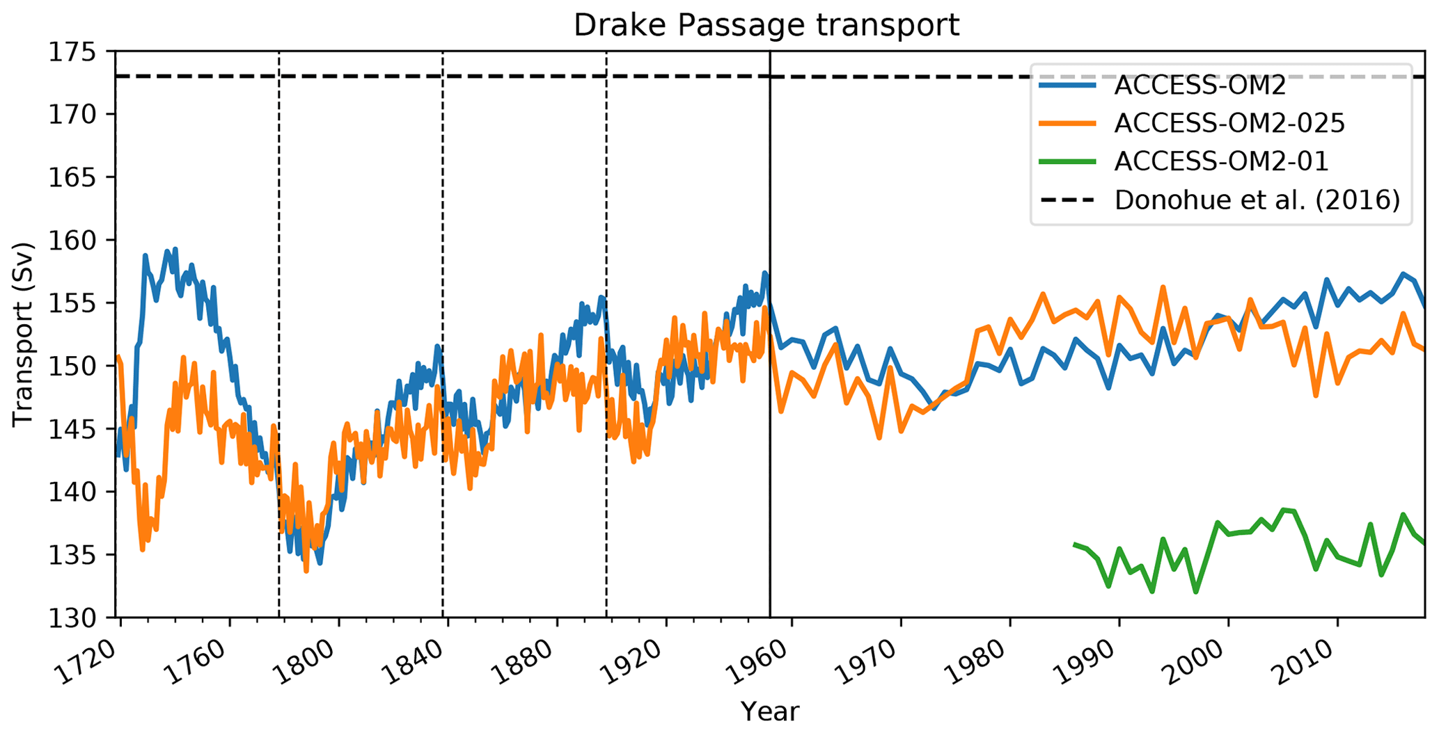
Figure 4Annual mean transport through Drake Passage as a function of time for each of the three model simulations. The horizontal black dashed line shows the observational estimate of Donohue et al. (2016). The vertical solid line divides the first four cycles (on the left) from an expanded view of the final cycle (on the right), with vertical dashed lines marking the end of each forcing cycle.
To evaluate the capacity of the different model configurations to represent the mean state of the broad-scale horizontal ocean circulation, the simulated mean dynamic sea level (MDSL) is compared to the CNES-CLS13 mean dynamic topography (MDT) observational product distributed by AVISO. Both the MDSL and MDT data are averages over the years 1993–2012. The global MDT product is a time mean that combines data from satellites, surface drifters, and in situ measurements, as described by Rio et al. (2011). The comparisons between the simulated MDSL and observed MDT (Fig. 5) indicate broad-scale agreement in this metric. There is a noticeable improvement in western boundary current structure in the higher-resolution models but a shallower MDSL minimum near Antarctica in the ACCESS-OM2-01 case, consistent with the reduced Drake Passage transport relative to observations (Fig. 4).
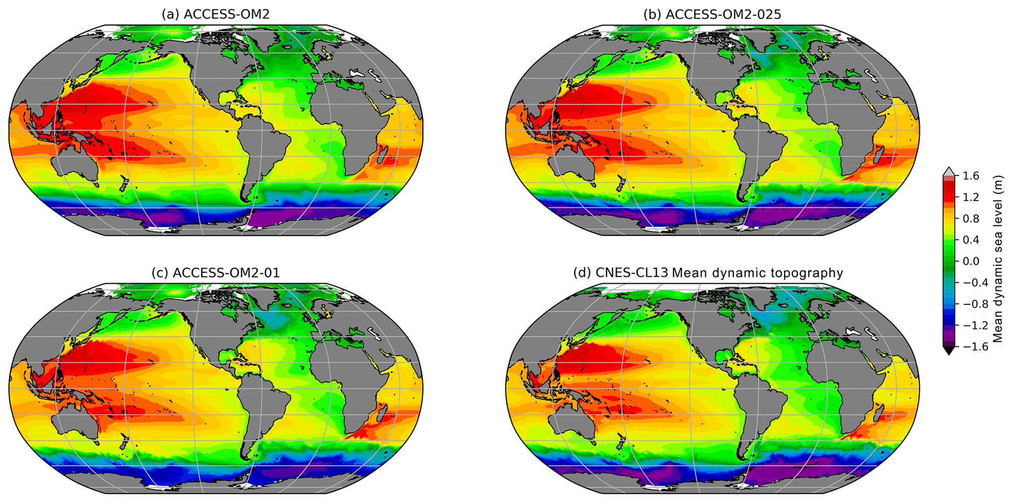
Figure 5The 1993–2012 mean dynamic sea level in (a) ACCESS-OM2, (b) ACCESS-OM2-025, and (c) ACCESS-OM2-01. (d) Observational reconstruction of 1993–2012 mean dynamic topography from the CNES-CLS13 product. The model outputs have had a 0.5 m offset added for clarity.
The capacity of the different model configurations to represent the spatial patterns of sea level variability provides a reliable proxy for surface mesoscale activity. To do this, we compute the standard deviation of the sea level anomaly (SLA) for each configuration at each model grid point to produce global maps of SLA deviation for the years 1993–2014 (from which long-term linear trends are removed). The simulated SLA standard deviation is then compared with the objectively interpolated, multi-mission, satellite-derived SLA product (AVISO SSALTO/DUACS), also from 1993–2014. We use the gridded observational product for convenience in comparing global maps of SLA variability. However, we note that the optimal interpolation procedure used to produce the gridded product from satellite ground tracks tends to smooth the underlying fields and hence may underestimate the SLA variance by as much as 50 % in certain regions (Chambers, 2018). As such, the true SLA variability may be higher than is indicated here.
The maps of SLA standard deviation are plotted in Fig. 6. Elevated SLA variability typically occurs in regions rich in energetic mesoscale eddies. For example, the altimetric product (Fig. 6d) shows elevated SLA variability in western boundary currents and their jet extensions, as well as in the Southern Ocean, which are regions where mesoscale dynamics are most active. Both the ACCESS-OM2-01 and ACCESS-OM2-025 simulations appear to capture this spatial pattern of SLA variability well, with both boundary currents and the Southern Ocean playing host to regions of enhanced SLA standard deviation. However, the ACCESS-OM2-025 configuration is unable to capture the magnitude of the observed variability, with values a factor of 2 or more below those of the observational product (which is itself an underestimate). The SLA variability magnitude in ACCESS-OM2-01 is closer to the observational estimate, but it is still somewhat low and with a differing pattern in the Gulf Stream region (discussed further in Sect. 4.2.4); the highest values are found south of the African continent in the Agulhas retroflection region, the Gulf Stream, and Kuroshio extension. As expected, the ACCESS-OM2 configuration is unable to represent any significant SLA variability, since eddies are parameterized rather than explicitly resolved in this coarse-resolution model.
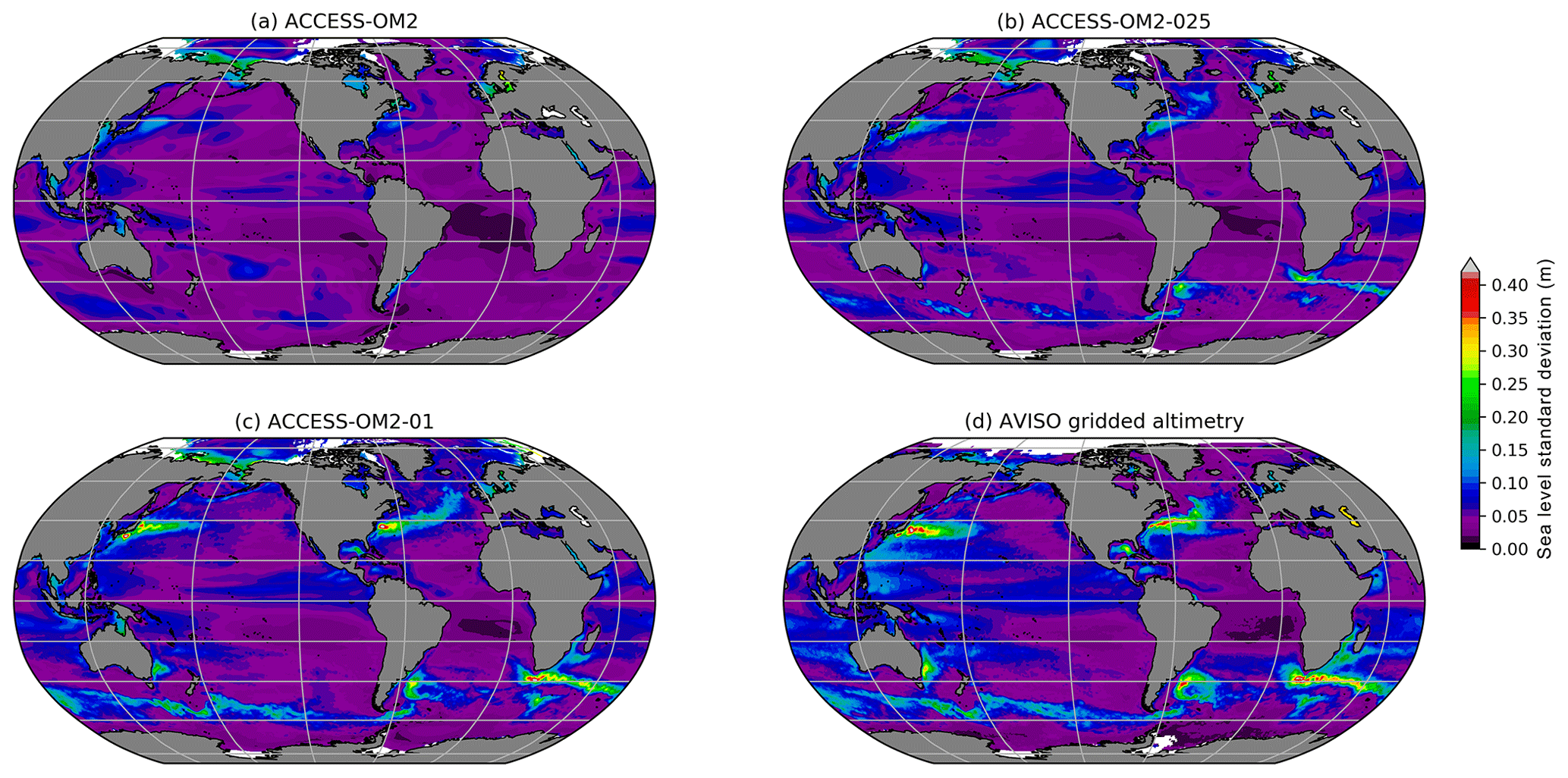
Figure 6Standard deviation of sea level anomaly η for the years 1993–2014. (a) ACCESS-OM2, (b) ACCESS-OM2-025, (c) ACCESS-OM2-01, and (d) AVISO SSALTO/DUACS gridded analysis of satellite altimetry. The model standard deviations are calculated from using the time means of η and η2 diagnosed at every baroclinic time step and therefore contain all model timescales.
Figure 6d also shows broad regions of enhanced sea level variability at lower latitudes, with less amplitude than the western boundary currents. These patterns are typically associated with slower modes of climate variability. El Niño–Southern Oscillation (ENSO) cycles drive variability in the eastern equatorial Pacific as well as in the western Pacific east of the Philippines and Papua New Guinea (Han et al., 2017; Mu et al., 2018). All resolutions simulate these patterns of variability associated with ENSO, though they all underestimate the observed variability by 10 %–20 %. In the Indian Ocean, variability is associated with both the Indian Ocean Dipole and ENSO (Li and Han, 2015). Anomalies in the tropical southern Indian Ocean (5–15∘ S, 60–80∘ E) are driven by ENSO-related wind anomalies (Xie et al., 2002), and the associated pattern of variability is simulated in each model resolution. Enhanced variability from the coasts of Indonesia (Potemra and Lukas, 1999) and the West Australian coast in Fig. 6d extends westward into the Indian Ocean due to Rossby wave propagation. The pattern of variability in ACCESS-OM2-01 is consistent with this, although somewhat weaker, whereas the pattern is much more muted in the coarser-resolution simulations.
4.1.2 Overturning circulation
Figure 7 shows the overturning circulation computed on potential density surfaces (referenced to 2000 dbar) and averaged over the last 25 years of simulation (1993–2017) for each of the three cases. In this figure the positive cell, which has a maximum near potential density 1036.5 kg m−3, is the inter-hemispheric upper overturning cell, which is dominated by the Atlantic component. This Atlantic Meridional Overturning Circulation (AMOC) involves the sinking of dense water in the North Atlantic, which re-emerges at the surface in the Southern Ocean (Marshall and Speer, 2012). There are clear differences between the three resolutions in their ability to represent the AMOC cell, which has an estimated transport from 2004 to 2012 of 17.2 Sv at 26∘ N (McCarthy et al., 2015). In ACCESS-OM2, the AMOC at 26∘ N is weak, with a maximum value of around 10 Sv, but it retains a strong inter-hemispheric character. In ACCESS-OM2-025 and ACCESS-OM2-01 the AMOC is considerably stronger, with the maximum value of the circulation only weakly decaying with latitude. A time series of the AMOC, measured at 26∘ N and constrained to the Atlantic basin only, clearly shows these differences (Fig. 8a) but also shows a decline over the duration of the ACCESS-OM2-01 case. The comparison of the AMOC in ACCESS-OM2-025 and ACCESS-OM2-01 with the years of McCarthy's estimate is favourable, although we cannot determine from the ACCESS-OM2-01 simulation whether this agreement will persist in future cycles. (Note that the first cycle of ACCESS-OM2-025 has a lower AMOC of ∼14 Sv; data not shown). Longer simulations are required before we can firmly establish the equilibrium behaviour of the AMOC for ACCESS-OM2-01.

Figure 7Time-mean zonally integrated overturning circulation computed on potential density surfaces (referenced to 2000 dbar) for (a) ACCESS-OM2, (b) ACCESS-OM2-025, and (c) ACCESS-OM2-01 simulations. Overturning is computed on density surfaces, integrated zonally around the globe and averaged over the last 25 years of simulation (1993–2017). The contour interval is 2 Sv, and the density axis is non-uniform.
The other circulation cell of interest in Fig. 7 is the abyssal overturning cell (the negative cell centred at 1037 kg m−3), which occupies a small part of density space but comprises a significant fraction of global water volume. Here, the strongest modelled overturning cell is in ACCESS-OM2-01 (12–15 Sv at 40∘ S, see Fig. 8b; compared with poorly constrained observational estimates of 20–50 Sv; Sloyan and Rintoul, 2001; Lumpkin and Speer, 2007; Talley, 2013). We argue that in ACCESS-OM2-01, this abyssal cell is partly driven by the more realistic process of surface water mass transformation on the Antarctic continental shelf (data not shown). On the other hand, the ACCESS-OM2-025 and ACCESS-OM2 abyssal cells are more dependent on water mass transformation due to open-ocean convection, but this dense water is poorly connected with the rest of the global ocean, leading to a weaker (∼6–10 Sv) overturning transport at 40∘ S. These biases in water mass transformation are common in coarse-resolution ocean and climate models (e.g. Heuzé et al., 2015a), indicating the potential of ACCESS-OM2-01 to be used for studies into the abyssal cell sensitivity to changes in climate. Overturning biases are further discussed in Sect. 4.1.4.
4.1.3 Ocean heat uptake
The evolution of global mean ocean temperature (Fig. 3a) is shown in more detail as horizontally averaged temperature anomalies in Fig. 9. Behaviour in the upper ocean (<100 m), the mid-depths (100–1500 m), and the abyssal ocean (>1500 m) is distinct. In ACCESS-OM2 and ACCESS-OM2-025, warming at mid-depth and cooling in the abyssal ocean are consistent with Bi et al. (2013b). These opposing trends largely cancel in ACCESS-OM2 but produce a net warming in ACCESS-OM2-025, which was established in the four cycles prior to the one shown (Fig. 3a). For these experiments, the evolution of temperature anomalies is similar for the full 300-year simulations (not shown), from which we infer that model drift dominates the temperature bias. The temperature drifts at mid-depths and abyssal depths in ACCESS-OM2-01 have opposite sign to the coarser models, with cooling at mid-depth (centred at 300 m) and weak warming in the deep ocean. The spatial structure of these drifts is shown in Figs. 10 and 12 (a, c, e) and is discussed further in Sect. 4.1.4.
Differences in temperature drift between different resolutions of the same ocean model component are usually due to differing resolved and parameterized processes. Previous studies with the GFDL-MOM CM2 suite (which shares a similar ocean model component with ACCESS-OM2) showed a consistent pattern of model drift across model resolutions (with the 0.25∘ warming the fastest), although in the coupled system all models warmed at a more rapid rate (Griffies et al., 2015). In particular, the warming tendency at mid-depths is larger when the mesoscale eddy processes (namely eddy advection and isoneutral diffusion) are not well-resolved. This especially occurs in eddy-permitting models (such as GFDL-MOM CM2.5, 0.25∘) which neither fully resolve eddy processes nor include any eddy parameterization. Our 0.25∘ model (ACCESS-OM2-025) includes both eddy advection (Gent and McWilliams, 1990) and neutral diffusion (Redi, 1982; Griffies et al., 1998) parameterization with weak coefficients which act to limit mid-depth warming (not shown), although it still has larger mid-depth drift than ACCESS-OM2.
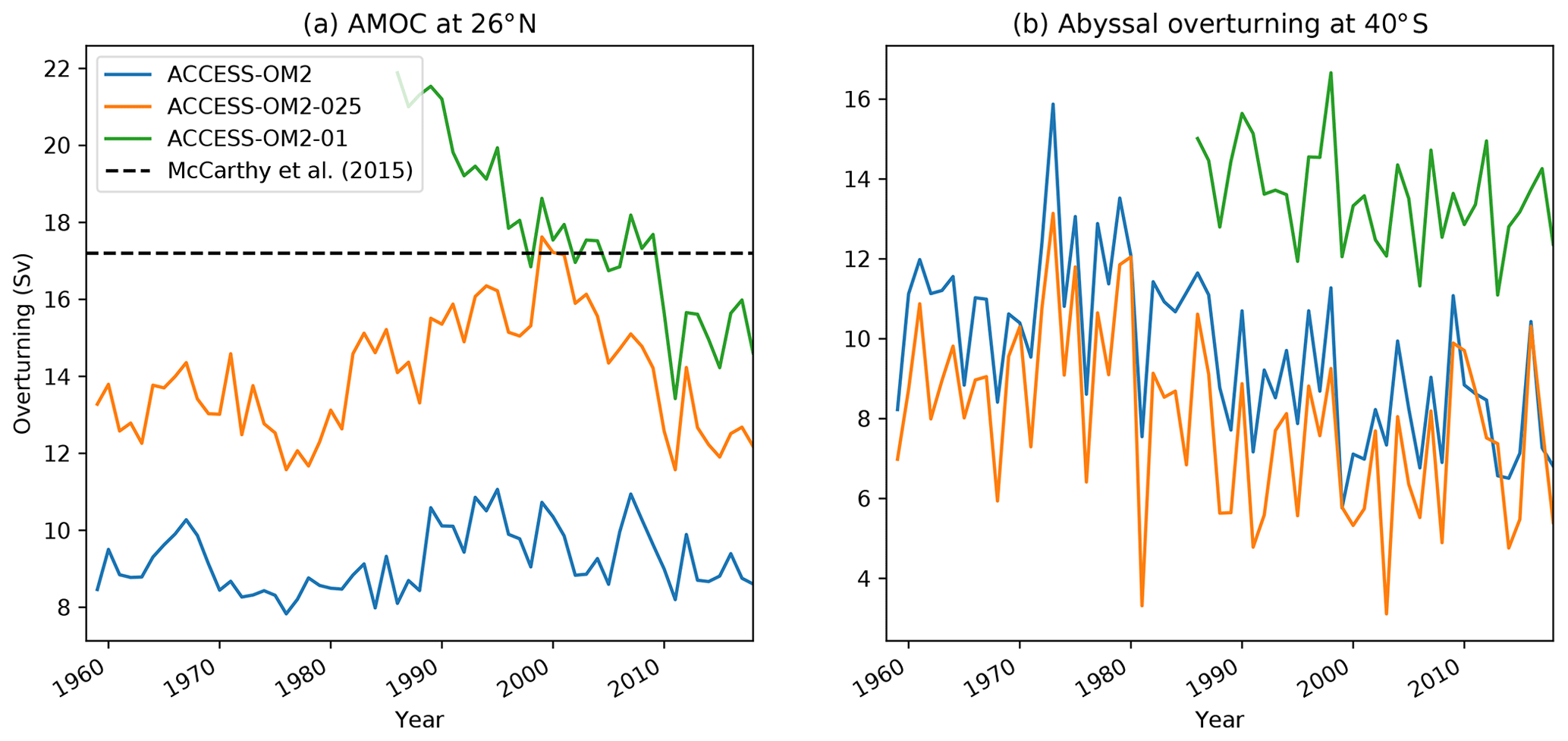
Figure 8(a) Annual mean upper overturning cell (AMOC) magnitude as a function of time, defined as the maximum value of the global overturning streamfunction computed on density surfaces, measured at 26∘ N, integrated between 103 and 5∘ W and for potential density classes that exceed 1035.5 kg m−3. The observational estimate from McCarthy et al. (2015) for 2004–2012 is shown by the dashed black line. (b) Annual mean abyssal cell overturning magnitude as a function of time, defined as the minimum value of the global overturning streamfunction computed on density surfaces, measured at 40∘ S, integrated zonally around the globe and for potential density classes exceeding 1036 kg m−3; its sign is changed to yield a positive value.
Differences in mesoscale eddy processes can account for quantitative differences in model drift, but the distinct temperature drift in ACCESS-OM2-01 is intriguing. Additional experiments with ACCESS-OM2 and ACCESS-OM2-025 following the same spin-up strategy used in ACCESS-OM2-01 (i.e. forced with JRA55-do 1984–1985 repeat-year forcing) reveal a temperature drift generally colder than the equivalent interannually forced experiments, especially in the upper 1000 m (not shown). These experiments suggest that the different spin-up approach in the ACCESS-OM2-01 simulation partially drives the mid-depth cooling observed at that resolution; differences in resolved and/or parameterized processes (including differences in the level of numerical mixing; Holmes et al., 2019) might play a secondary role.
Model drift dominates the long-term evolution of temperature anomalies, but considerable interannual variability occurs in the upper 100 m (Fig. 9). Warming trends toward the end of the historical period are superimposed upon the cold anomalies near the surface in all ACCESS-OM2 models. Atmospheric forcing such as Coordinated Ocean–Sea ice Reference Experiment (CORE) Interannual Forcing (IAF) and JRA55-do are not designed to reproduce a long-term trend as expected from climate change due to the adjustment performed to obtain a global surface heat budget closure over the satellite era (Tsujino et al., 2018). However, an inter-model comparison study under the CORE-IAF protocol showed that all models experienced an increase in ocean heat content in the upper 700 m and associated sea level rise over the 1993–2007 period similar to observations (Griffies et al., 2014). A practical approach to isolate the interannual variability from the model drift in ocean–sea ice model studies is to perform a de-drift using a control run, in a similar way as performed in fully coupled climate models (Sen Gupta et al., 2013; Hobbs et al., 2016). Whilst the protocol of CORE-IAF/JRA55-do does not require a control run, it can be achieved using a normal-year forcing (CORE-NYF) or a repeat-year forcing (JRA55-do).
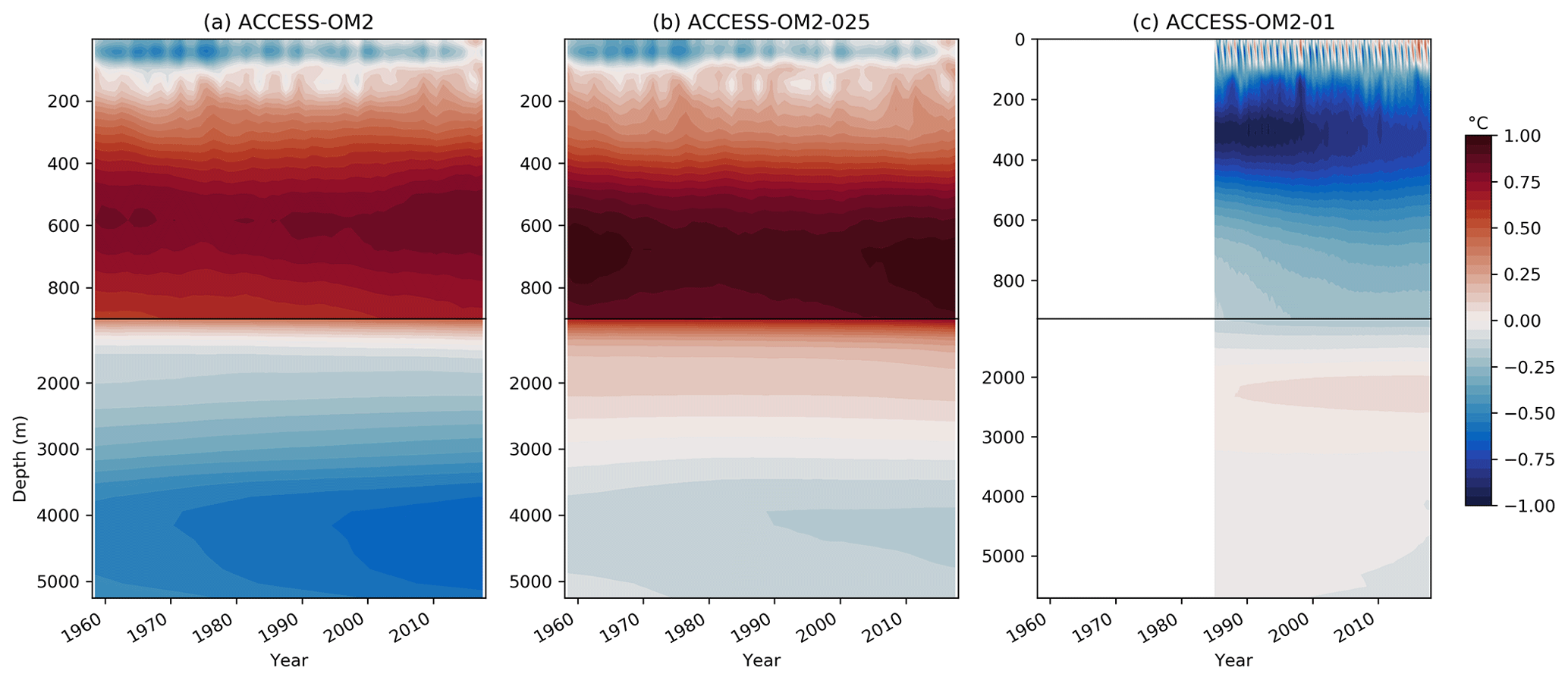
Figure 9Horizontally averaged temperature anomaly (∘C) relative to WOA13 as a function of depth and time over the last interannual forcing cycle for (a) ACCESS-OM2, (b) ACCESS-OM2-025, and (c) ACCESS-OM2-01. Panels (a) and (b) are annual means, and (c) shows monthly means.
4.1.4 Temperature and salinity biases
Model drift can occur for a variety of reasons in an ocean–sea ice model, particularly due to deficiencies in model physics and numerics or due to unresolved processes in the model coupling (Sen Gupta et al., 2013). This drift can be further investigated by examining model sea surface temperature (SST) biases (relative to WOA13 climatology) as presented in Fig. 10; the corresponding surface salinity (SSS) biases are shown in Fig. 11. Large warm biases associated with western boundary currents (WBCs) are found in all ACCESS-OM2 resolutions; this is also seen in many CORE models, associated with non-eddy-permitting resolution and poor representation of WBC separation and fronts (Griffies et al., 2009). These biases are reduced in ACCESS-OM2-025 and particularly in ACCESS-OM2-01; however, the similarities in the spatial pattern of surface temperature suggest the possibility of systematic biases in the surface forcing or in the surface coupling. ACCESS-OM2-01 does, however, differ from lower resolutions in the northern North Atlantic Ocean, with a stronger cold bias in the southern part of the subpolar gyre and a large-scale warm bias elsewhere; this is discussed further in Sect. 4.2.4.
In the Southern Hemisphere, larger biases in highly energetic regions (e.g. the Agulhas retroflection and along the ACC path) in ACCESS-OM2 appear to be due to an unrealistic representation of fronts, showing a significant improvement in the high-resolution experiments (ACCESS-OM2-025 and ACCESS-OM2-01). The biases in the Brazil–Malvinas confluence are much smaller at high resolution, probably due to a better representation of the eddy-driven Zapiola anticyclone (see Sect. 4.2.4 and Fig. 24).
The biases in the subpolar North Atlantic show significant differences across model resolution, likely due to details of the representation of the AMOC transport (see Sect. 4.1.2). The configurations with a strong AMOC (ACCESS-OM2-025 and ACCESS-OM2-01; see Figs. 7 and 8a) show negative temperature biases in the North Atlantic Current (NAC), which is (at least partially) density compensated by negative salinity biases (Fig. 11). Similar biases have been previously associated with a path of the NAC that is too zonal (Danabasoglu et al., 2014, and Sect. 4.2.4) and deficient overflow from the Nordic Seas (Zhang et al., 2011). ACCESS-OM2 has generally cold anomalies in the subpolar North Atlantic but comparatively smaller biases in the NAC; the weak AMOC transport is likely related to strong fresh biases around Greenland and in the Labrador Sea (Fig. 11).
ACCESS-OM2 presents a smaller warm bias near upwelling zones on the west coast of the American and African continents in comparison with CORE models (Griffies et al., 2009). This bias has been associated with coarse resolution in both model and wind stress forcing (Bi et al., 2013b) and may thus benefit from the higher horizontal resolution of the JRA55-do forcing in comparison with the CORE forcing (Taboada et al., 2019). However, this bias is larger in the high-resolution models (ACCESS-OM2-025 and ACCESS-OM2-01); the underlying cause of this bias is under investigation.
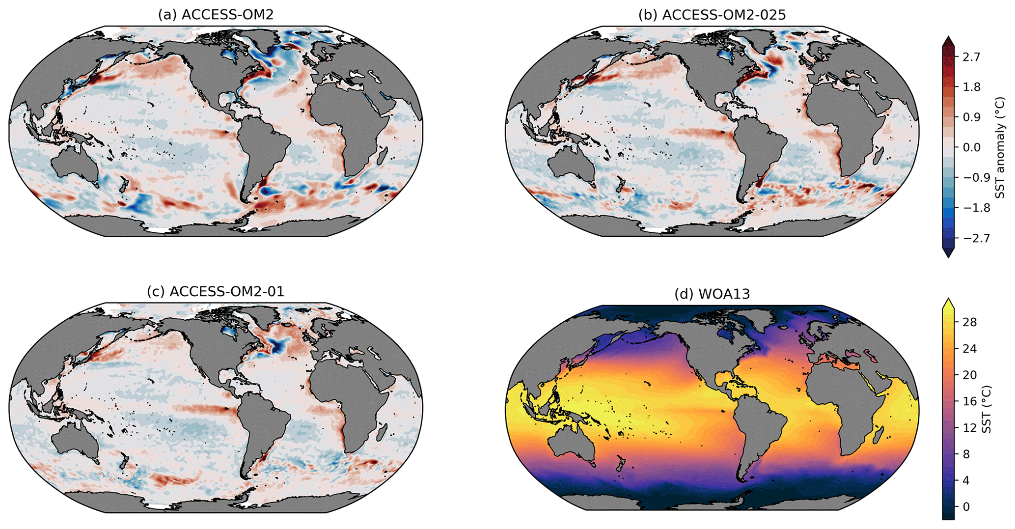
Figure 10Global 1993–2017 mean sea surface temperature (SST) bias relative to WOA13 for (a) ACCESS-OM2, (b) ACCESS-OM2-025, and (c) ACCESS-OM2-01. The WOA13 temperature field is shown in (d).
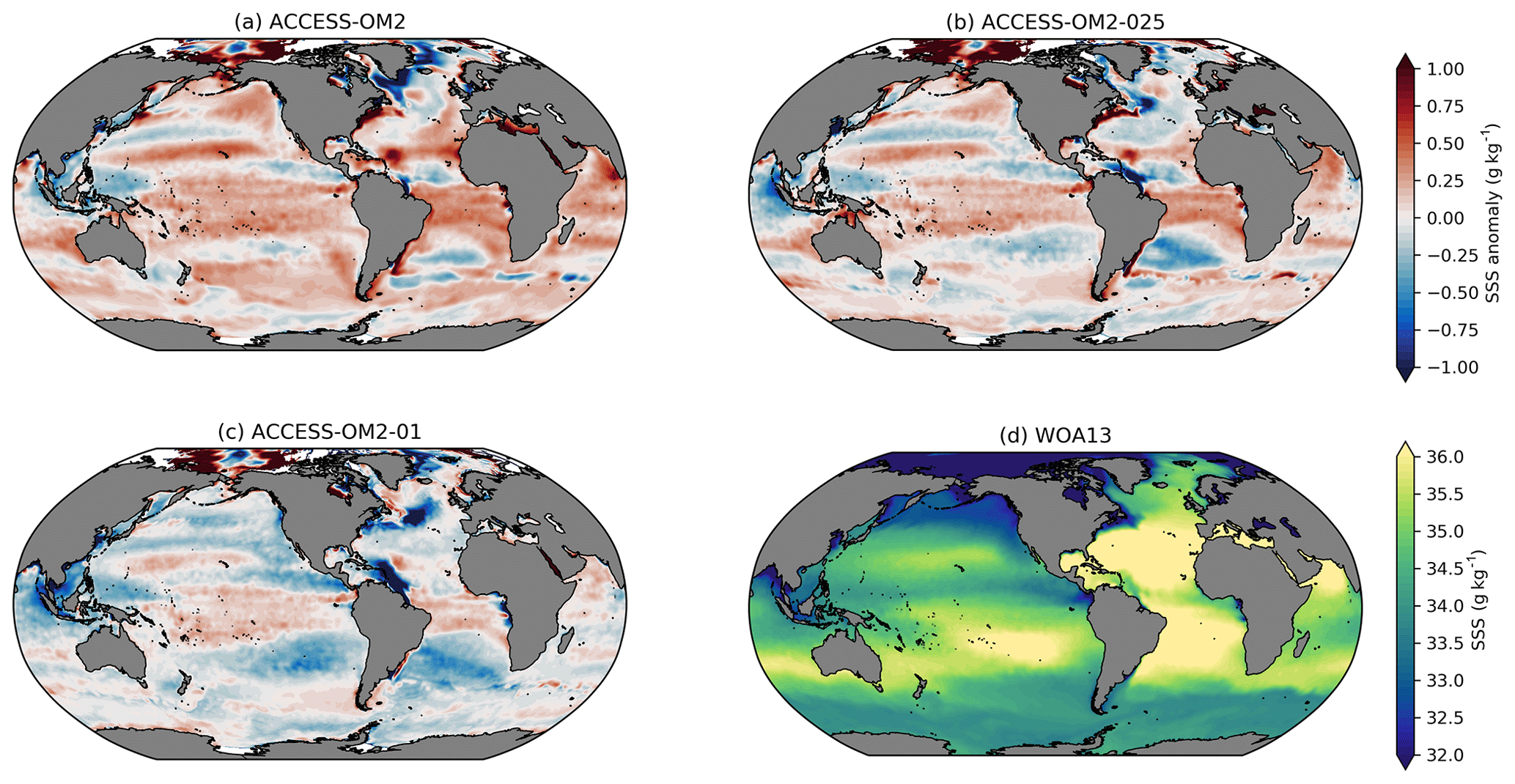
Figure 11Global 1993–2017 mean sea surface salinity (SSS) bias relative to WOA13 for (a) ACCESS-OM2, (b) ACCESS-OM2-025, and (c) ACCESS-OM2-01. The WOA13 salinity field is shown in (d).
The global zonal-mean anomalies of temperature and salinity relative to WOA13 are presented in Fig. 12. The distribution of heat and salt in the latitude and depth plane is controlled by the global thermohaline and wind-driven circulation. The difference between the model 1993–2017 mean in the last cycle and the observed climatology (WOA13) reveals geographical patterns of the model drift. In the Southern Ocean, the signature of Antarctic Bottom Water (AABW) shows a cold bias in ACCESS-OM2 and ACCESS-OM2-025 that spreads into the abyssal ocean. This bias is likely associated with large areas of anomalous deep (often full-depth) convection that appear every winter and spring in the eastern Weddell Sea and western Ross Sea in the ACCESS-OM2 and ACCESS-OM2-025 simulations. The behaviour of the two coarser models is typical of CMIP5 models, which produce bottom water by spurious deep-ocean convection rather than down-slope flows (Heuzé et al., 2013). In some models this convection is associated with spurious open-ocean polynyas (Heuzé et al., 2015b); however, as in the GFDL CM2.5 model (Dufour et al., 2017), persistent open-ocean polynyas do not form in the ACCESS-OM2 simulations. The deep cold bias is much reduced in ACCESS-OM2-01, which has a more realistic AABW formation in the Antarctic continental shelf, with anomalous open-ocean convection confined to a much smaller and more interannually variable region in the northeastern Weddell Sea (but has also had less time to drift away from climatology). The differences in Southern Ocean convection may partially explain the stronger ACC transport in the lower-resolution configurations (Fig. 4).
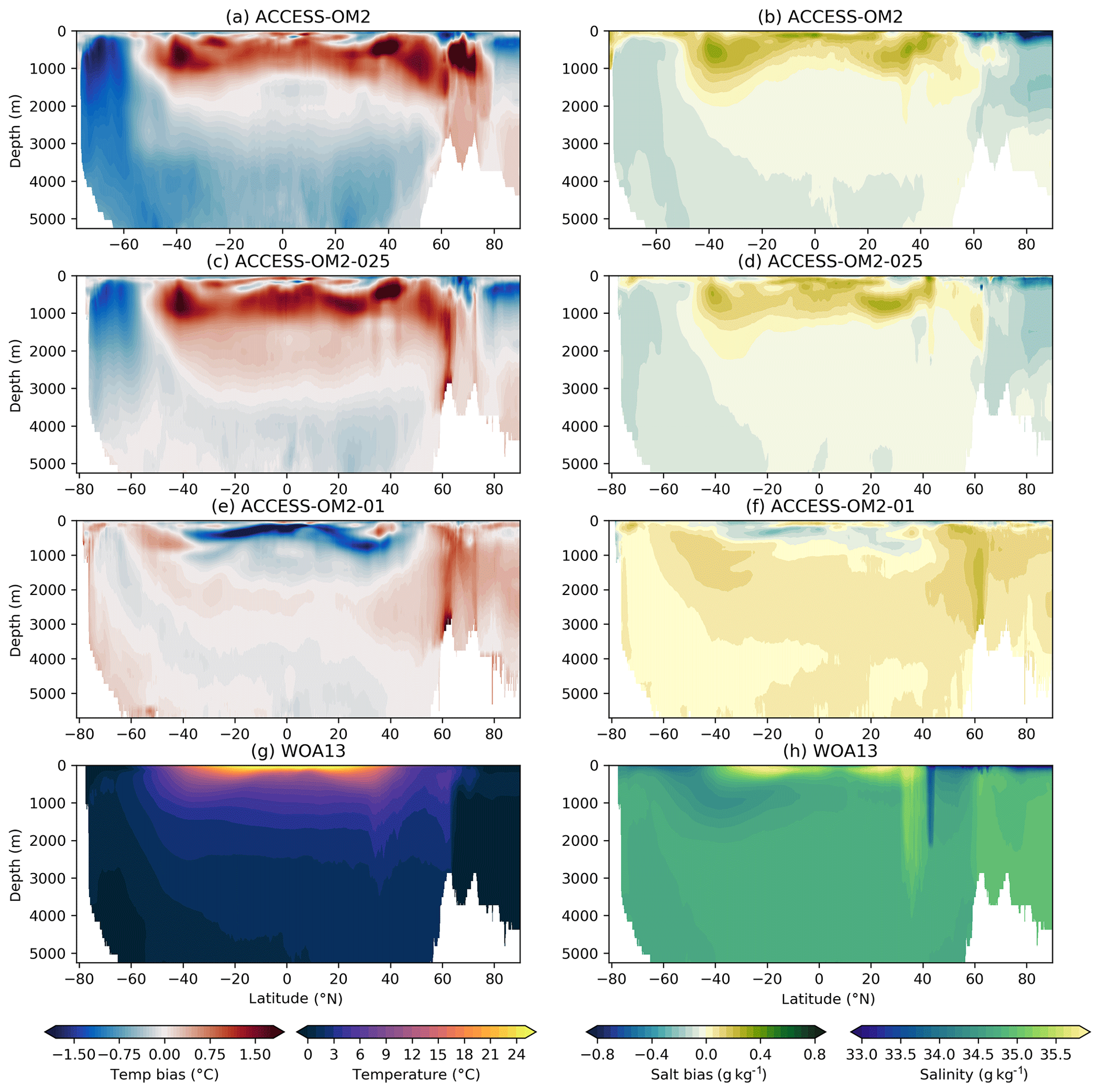
Figure 12Zonally averaged temperature bias relative to WOA13 for (a) ACCESS-OM2, (c) ACCESS-OM2-025, and (e) ACCESS-OM2-01. Zonally averaged salinity bias relative to WOA13 for (b) ACCESS-OM2, (d) ACCESS-OM2-025, and (f) ACCESS-OM2-01. The WOA13 zonally averaged temperature field is shown in (g), and the WOA13 zonally averaged salinity field is shown in (h). Model fields are 1993–2017 means.
The warm and salty biases north of 45∘ S above 1500 m are associated with weak penetration of cold and fresh Antarctic Intermediate Water, which can be caused by incorrect subduction and/or isopycnal mixing rates (Bi et al., 2013b). These biases are larger in ACCESS-OM2 and ACCESS-OM2-025 but smaller in ACCESS-OM2-01; we hypothesize that the coarser models have less isopycnal mixing (resulting from the sum of partially resolved and partially parameterized mixing), while ACCESS-OM2-01 seems to have a more realistic explicitly resolved isopycnal mixing. Weaker along-isopycnal transport may also drive positive temperature and salinity biases in the Northern Hemisphere at similar latitudes, resulting in a wide band of positive biases between 45∘ S and 45∘ N above 1500 m as a result of the isopycnal spreading of mode and intermediate water masses. These biases are significantly reduced in ACCESS-OM2-01, although it shows a considerable negative temperature and salinity bias at subsurface low latitudes (also seen in Figs. 19, 20, and 23). This bias in ACCESS-OM2-01 is possibly due to excessive upwelling of colder and fresher water from the ocean interior and/or insufficient mixing-driven downward heat transport because of the lack of vertical background diffusivity and reduced numerical diffusion in this configuration (Sect. 2.1.4), but further investigation is required.
The biases at high northern latitudes are linked to poor Gulf Stream behaviour (Sect. 4.2.4) and the Atlantic Meridional Overturning Circulation. In ACCESS-OM2-025 and ACCESS-OM2-01, wherein the AMOC transport is stronger (Figs. 7 and 8a), the zonal-mean bias shows warm anomalies between 1000 and 3000 m at 60∘ N (Fig. 12c, e). On the other hand, the weak AMOC transport in ACCESS-OM2 is translated into a strong warm bias above 1000 m, just below a large fresh bias (Fig. 12a, b). Warm biases in this region have been linked with excessive surface deep convective mixing and overturning (Griffies et al., 2009; Bi et al., 2013b).
4.1.5 Heat transport
All three model configurations reproduce the large-scale features of the meridional heat transport suggested by reanalysis products (Fig. 13). ACCESS-OM2 simulates a weaker northward heat transport than the other two configurations at most latitudes, associated with a weak AMOC (Figs. 7, 8). Heat transport within the Southern Ocean is consistent with observations within the spread between the observational products. Heat transport north of 40∘ N within ACCESS-OM2-025 and ACCESS-OM2-01 is stronger than suggested by the reanalysis products, but consistent within error bars with the more direct estimate from the World Ocean Circulation Experiment (WOCE) (Ganachaud and Wunsch, 2003). The local maximum in heat transport at ∼50∘ N is commonly seen in higher-resolution models and is thought to reflect a stronger Atlantic subpolar gyre contribution to the circulation (Griffies et al., 2015).

Figure 13Total meridional heat transport from each of the ACCESS-OM2 configurations (solid lines). Also included are observational estimates from Trenberth and Caron (2001), inferred from both NCEP (black crosses) and ECMWF (black dots) reanalysis data over the period February 1985–April 1989 (with error bars included for one of every five data points), and from the World Ocean Circulation Experiment (Ganachaud and Wunsch, 2003, red diamonds with error bars).
In the tropics, the models simulate consistently weak poleward heat transport in comparison to the reanalysis products in both hemispheres. This weak transport is a feature of many ocean-only and coupled climate models (e.g. Griffies et al., 2009, 2015). The ACCESS-OM2 configurations do not lie outside the range of model-simulated transports in this regard. There are well-known issues with inferring poleward heat transport from reanalysis products, and there are large variations between different products (e.g. Griffies et al., 2009; Valdivieso et al., 2017). Furthermore, the model simulations are more consistent with the inferred heat transport from the JRA55-do forcing itself at these low latitudes, particularly in the Southern Hemisphere (see Fig. 30 of Tsujino et al., 2018). The models still underestimate the peak in northward heat transport at 20∘ N (∼1.3 PW in ACCESS-OM2-025 and ACCESS-OM2-01 compared to ∼1.5 PW from the JRA55-do forcing). The reason for this mismatch remains unclear and is worthy of further investigation. Nonetheless, the results show that ACCESS-OM2-025 has a clear advantage over ACCESS-OM2 in representing heat transport at most latitudes, with the possible exception of 0–30∘ S.
4.2 Regional ocean circulation
The second part of this model evaluation involves examining the performance of the model at a selected number of key regions. In these regional analyses we will focus on the major circulation features such as the separation of western boundary currents, the average state of equatorial currents, and flow through major choke points. The regional evaluation is not intended to be comprehensive but will instead outline regions in which the model behaves well or poorly. It is envisaged that more in-depth analyses will be published using this model in the near future.
4.2.1 Southern Ocean
A significant motivation for moving towards high-resolution ocean models is to better represent the dynamics of the Southern Ocean, where mesoscale variability plays a critical dynamical role in the evolution of the system (e.g. Hogg et al., 2015). An example of the improvement in water mass properties can be seen in Fig. 14, where transects of temperature and salinity along the SR3 hydrographic line are compared with historical observations. Here, progressively enhancing the resolution leads to better representation of the observed surface low-salinity layer, enhanced subduction into the mid-depths, and improved Antarctic shelf properties and abyssal temperature–salinity structure (bearing in mind that the ACCESS-OM2-01 simulation is less well-equilibrated and thus has had less opportunity to drift away from the initial climatology).
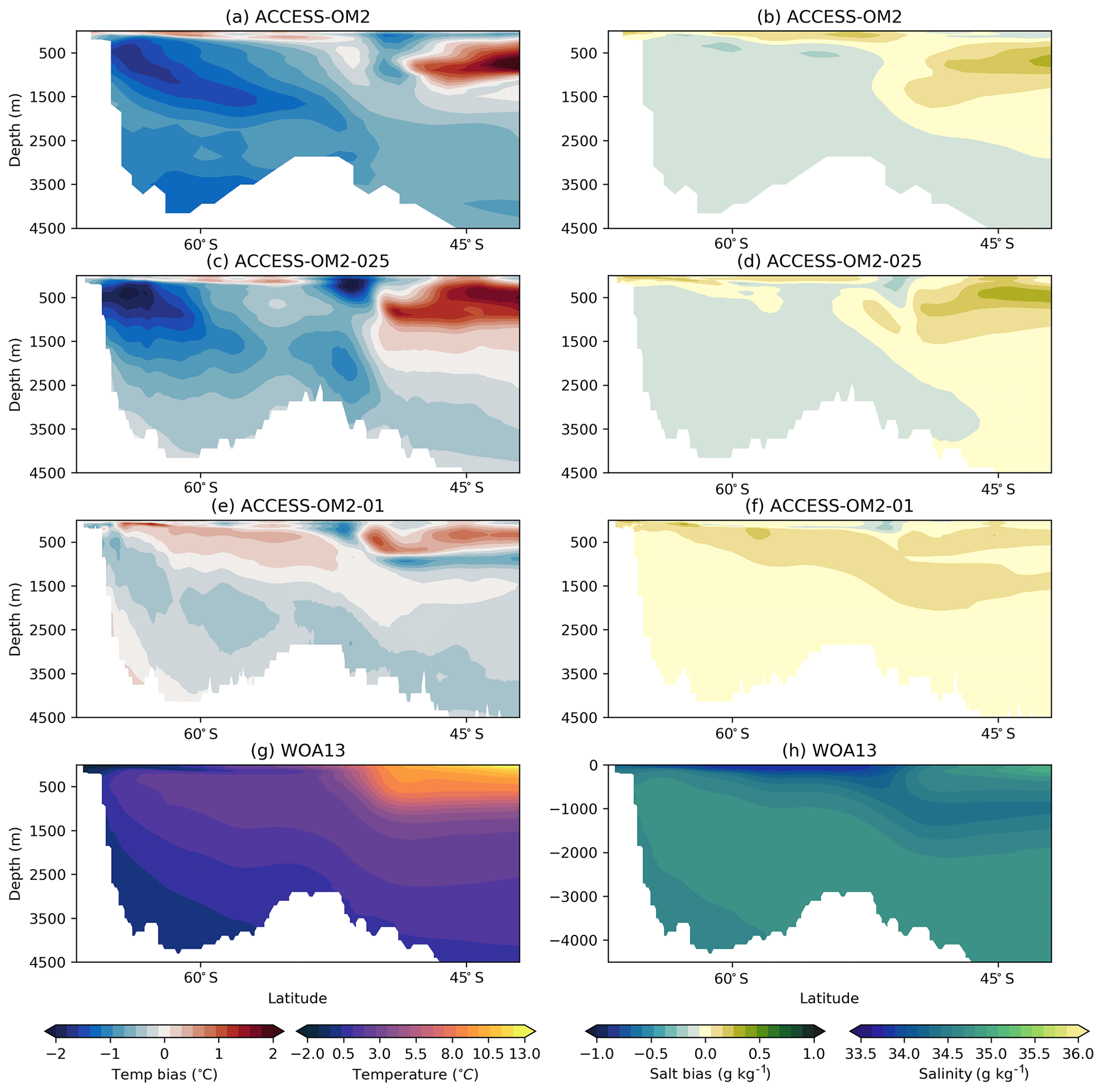
Figure 14Meridional transects of 1993–2017 mean potential temperature (left panels) and salinity (right panels) south of Tasmania, along longitude 150∘ W, near the WOCE/GO-SHIP repeat hydrographic line SR3 for (a–b) ACCESS-OM2, (c–d) ACCESS-OM2-025, (e–f) ACCESS-OM2-01, and (g–h) gridded climatologies from WOA13 for the period 1985–2013.
Figure 15 shows a meridional transect of planetary geostrophic potential vorticity (, where f is the Coriolis parameter, g is the acceleration due to gravity, ρ0 is the reference density, σ0 is the potential density anomaly referenced to 0 dbar, and z is the vertical coordinate, positive upwards) across a Subantarctic Mode Water (SAMW) formation region at 120∘ W. The blue lines show the maximum mixed layer depth (MLD) representative of the winter season when SAMW is ventilated, and black lines show the minimum MLD representative of the summer season. For all model resolutions, mixed layer depths are very similar. Nevertheless, maximum mixed layer depths are deeper than observations suggest, especially in ACCESS-OM2 and ACCESS-OM2-025 (data not shown). Bias in the MLD may be due to a number of factors, such as bias in the surface buoyancy forcing (Sallée et al., 2013), systematic errors in the convective parameterization, sub-grid-scale turbulence and friction schemes (Dufresne et al., 2013), the representation of submesoscales (Wenegrat et al., 2018), and the inability of the prescribed air temperature to adjust towards the SST, as would occur in a coupled ocean–atmosphere model. Determining the exact cause of the bias requires a careful analysis of the mixed layer budgets and is beyond the scope of this article.
Mean mixed layer depths are insensitive to model resolution, but the distribution of planetary geostrophic potential vorticity (PV) changes substantially: for the highest-resolution configuration, ACCESS-OM2-01, there are two distinct layers of high PV magnitude at depths of about 900 and 1400 m at 35–50∘ S separated by a slight minimum at about 1200 m, while in both ACCESS-OM2 and ACCESS-OM2-025 these spread in the diapycnal direction and merge into a single, somewhat deeper layer. At the same time, PV in the mode water layer increases in magnitude with increasing resolution. It is not clear from our current understanding of mode water ventilation how the uptake of tracers (e.g. heat and carbon) into the ocean interior will be affected by the excessive winter mixed layer depth and differences in the distribution of PV in these models.
Sea level variability in the region of the Agulhas Current is shown in Fig. 16 (colours) for each model resolution, including a comparison with observations. Variability follows the contours of the barotropic streamfunction (white contours) down the Mozambique channel (de Ruijter et al., 2002) and the eastern Madagascar coast, continuing along the southeast coast of southern Africa. There is a peak in variability in all simulations where the Agulhas Current retroflects at the southern tip of the African continental shelf. From here, variability continues both west into the South Atlantic basin along the path of the Agulhas rings (Dencausse et al., 2010) and east along the Agulhas Return Current. The peak in this variability is well-captured in the ACCESS-OM2-01 simulation relative to observations, whereas variability amplitudes in the ACCESS-OM2-025 simulation are about half those observed, and the variability in ACCESS-OM2 is substantially less again. The path of the circulation in the region before the retroflection, as indicated by the contours of the barotropic streamfunction, is consistent between the simulations and the observations. A sea level variability hotspot is well-captured to the south of the main retroflection in the ACCESS-OM2-01 simulation (around 48∘ S, 30∘ E) over the southwest Indian Ridge upstream of the Prince Edward Islands (Ansorge et al., 2012). ACCESS-OM2-025 also captures this feature with reduced amplitude, while it is missing in ACCESS-OM2.
4.2.2 Australasia
In the southwest Pacific Ocean the westward South Equatorial Current bifurcates at the Australian coast at about 16∘ S, with the southward branch forming the southward-intensifying East Australian Current (EAC). Between 33 and 35∘ S the EAC splits into an eddying eastward outflow (known as the Tasman Front) and the EAC extension, an alongshore southward-weakening eddy-dominated flow (Ridgway and Dunn, 2003). Sea level standard deviation in ACCESS-OM2-01 (Fig. 17c) reproduces the observed spatial distribution of eddy activity in this region (Fig. 17d) but underestimates its magnitude. The variability is more severely underestimated in the coarser configurations (Fig. 17a, b). ACCESS-OM2-025 retains a weak qualitative signature of both the Tasman Front and the EAC extension, whereas these are nearly absent in ACCESS-OM2.
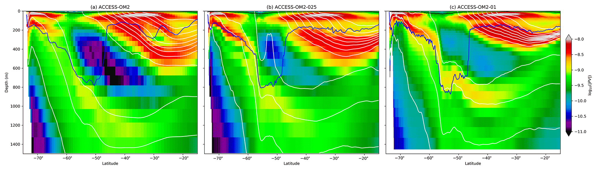
Figure 15Meridional transects of time-mean planetary geostrophic potential vorticity (PV; s−3) across a Subantarctic Mode Water (SAMW) formation region at 120∘ W in the three configurations. Colours represent , white lines represent σ0 (contour interval 0.25 kg m−3), and black (blue) lines represent the minimum (maximum) of the monthly mean mixed layer depth (defined by a 0.03 kg m−3 density criterion) over 1993–2017.
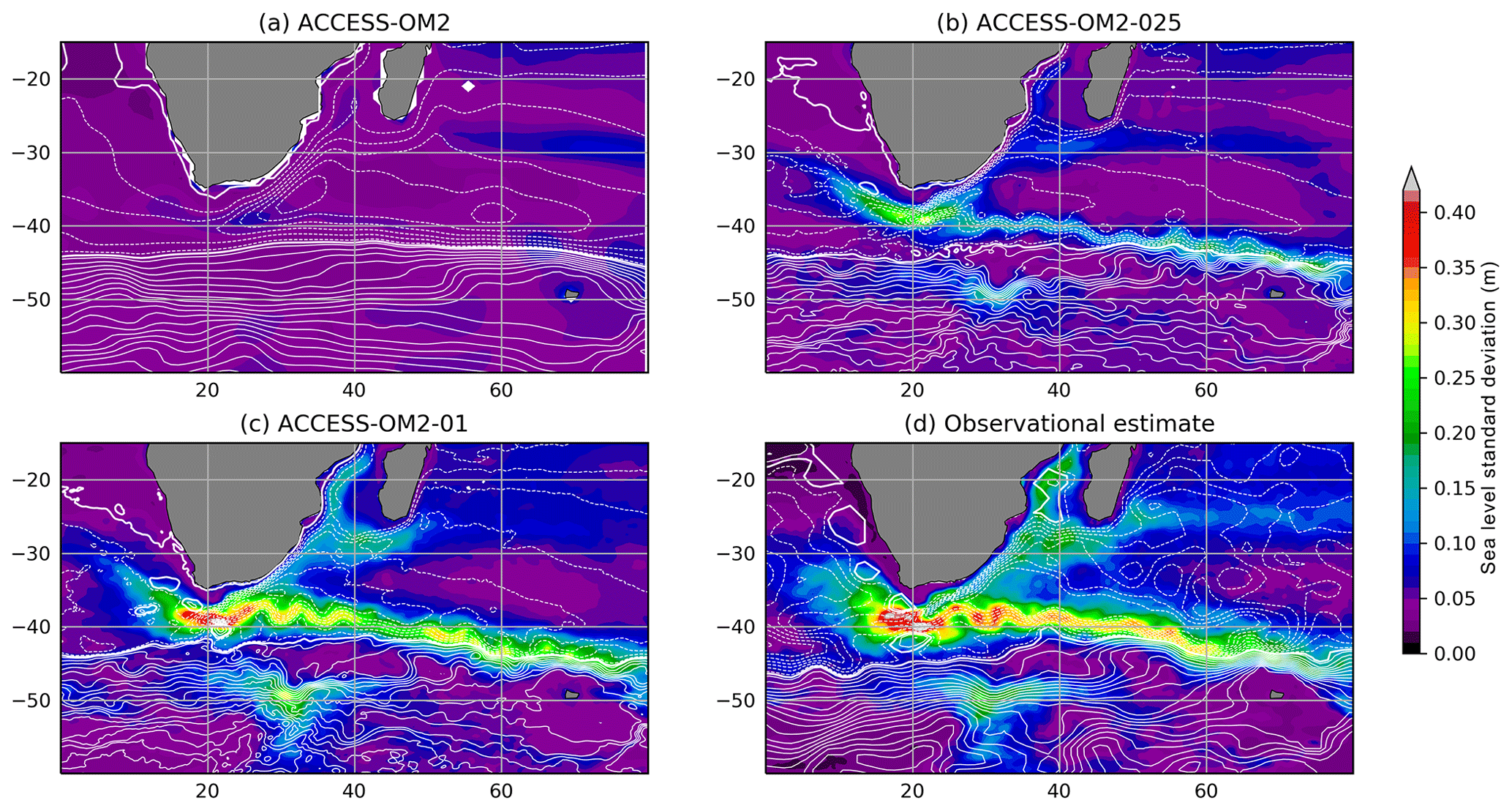
Figure 16Standard deviation of sea level anomaly (colours; model values calculated as in Fig. 6 but for 1993–2017) overlaid with contours of mean barotropic streamfunction (contour interval 10 Sv) in the Agulhas region for (a) ACCESS-OM2, (b) ACCESS-OM2-025, (c) ACCESS-OM2-01, and (d) AVISO SSALTO/DUACS gridded analysis of satellite altimetry (colours) and 1∘ gridded barotropic streamfunction contours estimated from hydrography and Argo displacements (Colin de Verdière and Ollitrault, 2016).
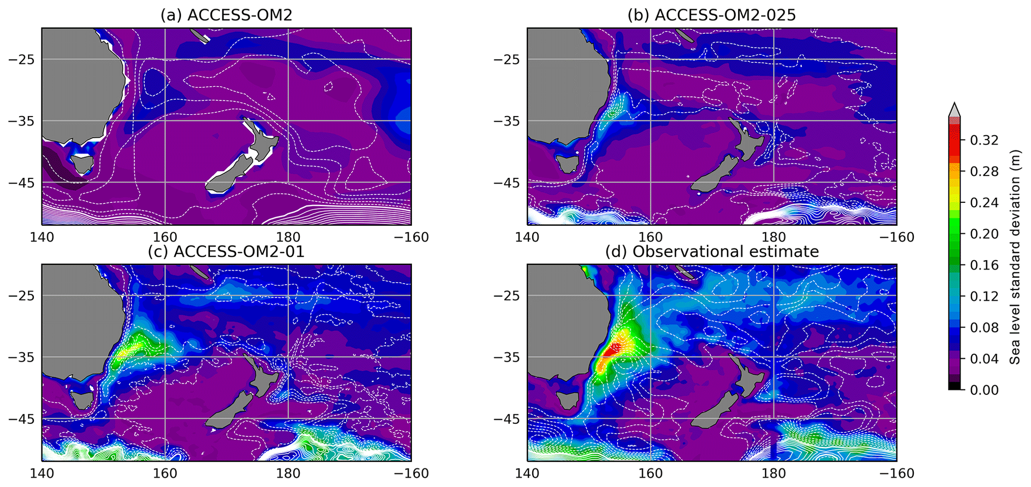
Figure 17Standard deviation of sea level anomaly (colours) and mean barotropic streamfunction (contours) as in Fig. 16 but for the East Australian Current region, with a different colour scale and streamfunction contour interval of 5 Sv.
The contours of the barotropic streamfunction converge near Australia's east coast in observations (Fig. 17d), but the transport of the EAC is underestimated in all model configurations. Furthermore, the EAC broadens (as expected) with the reduction of horizontal resolution. The poleward-only 1993–2017 mean EAC transports above 2000 m at 28∘ S are 18.7, 17.5, and 17.2 Sv in ACCESS-OM2, ACCESS-OM2-025, and ACCESS-OM2-01 (respectively), somewhat weaker than 22.1 Sv observed by Sloyan et al. (2016) at 27∘ S. The South Equatorial Current is also weaker than observed (Sect. 4.2.3), suggesting a weak South Pacific wind-driven circulation in all ACCESS-OM2 models.
The Indonesian throughflow (ITF) from the Pacific Ocean to the Indian Ocean is the only tropical inter-ocean pathway in the global ocean circulation, and its magnitude through key straits is an important indicator of the fidelity of the model in this region. The total ITF transport in ACCESS-OM2-01 agrees well with INSTANT observations by Sprintall et al. (2009) (green and dashed lines in Fig. 18a), but the total transport is too weak in the coarser configurations. The detailed breakdown of transport through the three main straits (Lombok Strait, Ombai Strait, and Timor Passage; Fig. 18b–d) shows that there are compensating biases in individual straits in ACCESS-OM2-01, and the coarser configurations may overestimate or underestimate transport in each strait. Models may underestimate the magnitude of the total transport or the transport in individual straits for three primary reasons. Firstly, the ITF transport from the Pacific to the Indian Ocean is induced by the sea level gradient between these two oceans; in ACCESS-OM2 and ACCESS-OM2-025, this sea level gradient is weaker than observed and 10 % smaller than in ACCESS-OM2-01 (Fig. 5). Thus, it is not strong enough to reproduce the observed total transport. Secondly, the Lombok and Ombai straits are narrow (minimum width 20 and 40 km, respectively) and therefore require a high horizontal resolution to faithfully represent the strait transport. For example, the width of Lombok Strait is one velocity cell (∼110 km) in ACCESS-OM2, one cell (∼28 km) in ACCESS-OM2-025, and two cells (∼22 km) in ACCESS-OM2-01; Rayleigh drag (Sect. 2.1.4) is used in ACCESS-OM2 to obtain more realistic transport through the Lombok and Ombai straits. Thirdly, the ITF outflow is split between the three main straits flowing first through the Lombok Strait, then the Ombai Strait, and finally the Timor Strait. So if more of the water that comes through Makassar Strait goes through Lombok Strait (as in ACCESS-OM2-025), less water will go through the Timor Passage. As a consequence, the resolution of straits is critical for this region, and for this reason the ACCESS-OM2-01 configuration is more appropriate to study the Indonesian seas.

Figure 18Time series of annual-mean transport through the Indonesian straits. The total Indonesian throughflow (a) can be broken into (b) Lombok Strait, (c) Ombai Strait, and (d) Timor Strait. Black dashed lines indicate the mean throughflow during 2004–2006 from the INSTANT programme (Sprintall et al., 2009). Negative values indicate southward flow.
4.2.3 Pacific Ocean
All three versions of ACCESS-OM2 reproduce the major features of the equatorial Pacific Ocean circulation well compared with observations from Johnson et al. (2002) (Fig. 19), which are in turn similar to measurements from the TAO array on the Equator at 140∘ W and 165∘ E (not shown). The strength of the Equatorial Undercurrent (EUC) core is within 10 % of observations, and its latitudinal width at 140∘ W is accurate in ACCESS-OM2-025 and ACCESS-OM2-01 but somewhat too wide in ACCESS-OM2. The EUC extends too deeply in both ACCESS-OM2-025 and ACCESS-OM2-01. The strength of the thermocline is reproduced well in ACCESS-OM2 and ACCESS-OM2-025, although in ACCESS-OM2-01 it is slightly too strong. The strong Pacific thermocline in ACCESS-OM2-01 also appears in the zonal mean (Fig. 12) and Atlantic (Fig. 23); the cause of this bias is currently under investigation. The vertical temperature gradient above the thermocline appears to be too weak in all three configurations, a bias which may also be linked to the weak vertical shear in the upper EUC. Further, both the northern and southern branches of the South Equatorial Current (SEC, the westward surface-intensified current south of ∼5∘ N) are too weak in the models. These biases in the SEC and upper EUC may be associated with problems in the turbulent mixing parameterizations in this region, but a detailed sensitivity study has not yet been undertaken. The eastwards North Equatorial Counter Current (NECC) at 7∘ N is very weak in the models. A weak northern SEC branch and NECC are common biases in ocean models (e.g. Large et al., 2001; Tseng et al., 2016).
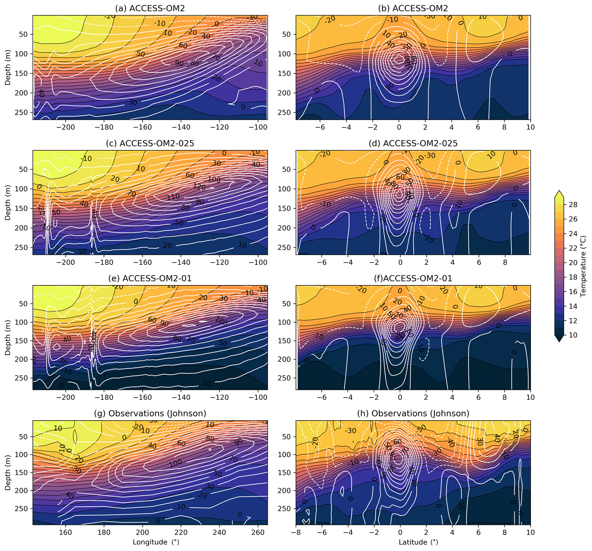
Figure 19Comparison of temperature (colour and contours every 1 ∘C) and zonal velocity (white contours every 10 cm s−1 with black labels in centimetres per second) along the Equator (left) and at 220∘ E (right) in the Pacific for (a–b) ACCESS-OM2, (c–d) ACCESS-OM2-025, (e–f) ACCESS-OM2-01, and (g–h) observations (Johnson et al., 2002).
Figure 20 shows meridional transects of the climatological means of potential temperature and salinity across the approximate centre of the basin at 150∘ W (near the WOCE/GO-SHIP repeat hydrography line P16) for each model configuration. For comparison, we include an observational estimate of the climatological mean along the same transect, taken from the gridded WOA13 product, for the period 1985–2013 (Fig. 20g, h). In general, all three model configurations produce a realistic thermal structure in this basin. In particular, the models capture the approximate depth of the thermocline and its inter-hemispheric asymmetry (with the Southern Hemisphere thermocline being somewhat deeper than in the Northern Hemisphere), the strong temperature gradients in the Southern Ocean at approximately 55∘ S coincident with the location of the Antarctic Circumpolar Current, and the weak vertical gradients to the north of the ACC in the regions associated with Southern Hemisphere mode water production. However, at approximately 50∘ S, this region of weakly stratified water is substantially deeper in the high-resolution ACCESS-OM2-01 simulation than in the ACCESS-OM2 and ACCESS-OM2-025 configurations or the WOA13 observations, which is suggestive of the overproduction of Subantarctic Mode Water.

Figure 20Meridional transects of 1993–2017 mean potential temperature (upper panels) and salinity (lower panels) in the central Pacific Ocean, along longitude 150∘W, near the WOCE/GO-SHIP hydrographic line P16 for (a–b) ACCESS-OM2, (c–d) ACCESS-OM2-025, (e–f) ACCESS-OM2-01, and (g–h) gridded climatologies from WOA13 for the period 1985–2013.
In contrast to the temperature structure, which was simulated reasonably well by the various models in this suite, the meridional haline structure of the central Pacific is not well-simulated. In particular, none of the models reproduce the observed deep salinity minimum in either hemisphere, although there is some suggestion of the penetration of relatively fresh waters into the interior at approximately 55∘ S and 45∘ N in the ACCESS-OM2-025 and ACCESS-OM2-01 configurations. As such, it is possible that the models' representation of Pacific mode and intermediate waters will be affected by the poor representation of the deep salinity structure, which could, in turn, have implications for the local overturning circulation (Thompson et al., 2016).
Figure 21 shows sea level variability and barotropic streamfunction in the North Pacific, including the region of the Kuroshio Current. ACCESS-OM2 simulations at each resolution show variability focused near the separation from the coast of Japan, decaying eastward along the Kuroshio extension. However, the observed variability continues with significant amplitude further along the extension. Peak variability here in ACCESS-OM2-01 matches the observed amplitude (∼0.4 m), whereas ACCESS-OM2-025 has a reasonable distribution of variability with reduced magnitude (peak ∼0.25 m), and ACCESS-OM2 substantially underestimates this (0.15 m). ACCESS-OM2-01 has variability upstream of the separation point, higher than that observed, where the Kuroshio's “large meander” appears on interannual timescales (Kawabe, 1995). In ACCESS-OM2-01 the barotropic streamfunction has a similar structure to the observational estimate but seems somewhat weaker in amplitude (white contours in Fig. 21c, d). The directly observed mean Kuroshio transport on the WOCE PCM-1 line between Taiwan and the southern Ryukyu Islands was 21.5±2.5 Sv between September 1994 and May 1996 (Johns et al., 2001). Corresponding transports over the same period are close to this value in ACCESS-OM2-025 and ACCESS-OM2-01 (17.5 and 20.1 Sv, respectively) but much weaker (7.6 Sv) in ACCESS-OM2, which is lower than in other models of this resolution under CORE-II forcing (Tseng et al., 2016).
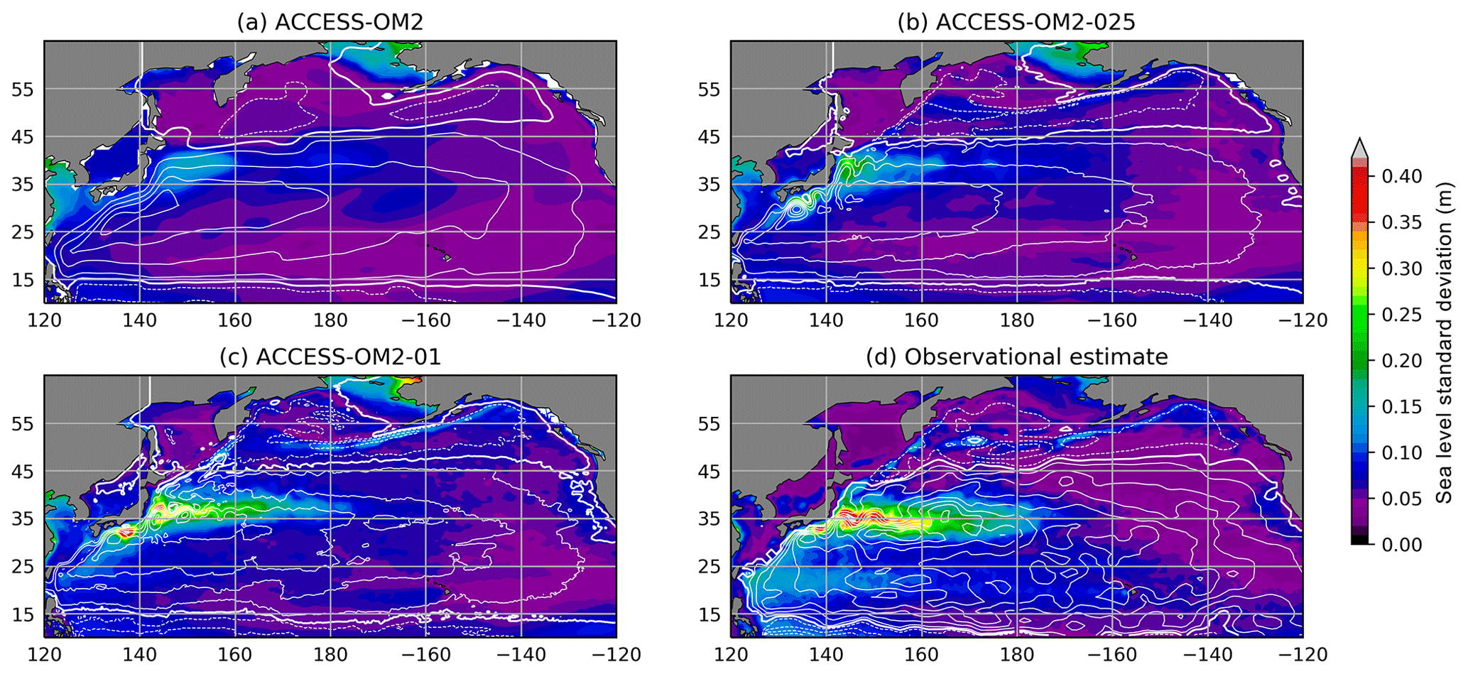
Figure 21Standard deviation of sea level anomaly (colours) and mean barotropic streamfunction (contours) as in Fig. 16 but for the Kuroshio region.
4.2.4 Atlantic Ocean
Accurately representing the horizontal circulation of the North Atlantic is a persistent challenge for ocean modellers. In particular, models commonly fail to simulate a Gulf Stream that separates from the North American coast at Cape Hatteras (35∘ N, 75∘ W) and a North Atlantic Current that flows north along the east side of the Grand Banks from 40 to 51∘ N (Rossby, 1996; Chassignet and Marshall, 2008). In ACCESS-OM2 and ACCESS-OM2-025, the Gulf Stream flow is too weak and overshoots the separation latitude by about 4∘ relative to observations (Fig. 22a, b). In ACCESS-OM2-025 the separation latitude is also highly variable. The Gulf Stream structure in ACCESS-OM2-01 appears much closer to observations (Fig. 22c); however, the situation is more complex than this time mean suggests. Between 1985 and about 2008 the ACCESS-OM2-01 Gulf Stream generally separates at or slightly north of Cape Hatteras, but the path of the separated current gradually changes from eastward to northeastward (not shown). After about 2008 the Gulf Stream adopts a configuration similar to ACCESS-OM2-025 (Fig. 22b), usually separating about 4∘ too far north, with a compact anticyclonic recirculation immediately south of the separated current (not shown). This long-term shift appears as excessive sea level variability shortly after separation and broadening of the separated jet in the long-term mean relative to observations (Fig. 22c, d). None of these models adequately capture the northward flow of the North Atlantic Current along the east side of the Grand Banks, resulting in significant cold and fresh biases in the sea surface temperature and salinity (Figs. 10 and 11). These biases qualitatively resemble those of Griffies et al. (2015) but contrast with other studies (e.g. Bryan et al., 2007; Storkey et al., 2018) which found significant improvement in the Gulf Stream's separation and path around the Grand Banks at high resolution (although Bryan et al., 2007, found that this also required low viscosity). The cause of Gulf Stream misbehaviour in the ACCESS-OM2 models is currently under investigation. Among the possible culprits are a weak deep western boundary current (Zhang et al., 2011) and low inertia (Özgökmen et al., 1997).
ACCESS-OM2-025 and ACCESS-OM2-01 simulate the Loop Current in the Gulf of Mexico (although with lower variability than the altimetric estimate), which flows through the Florida Straits to join the Florida Current and Gulf Stream. In contrast, the Caribbean circulation is incorrect in ACCESS-OM2, with the gyre circulation closed primarily via the Bahamas rather than the Florida Straits. Transport between Florida and Grand Bahama at 27∘ N is 23.4 Sv in ACCESS-OM2-025 and 20.4 Sv in ACCESS-OM2-01, significantly weaker than the observed 32.1 Sv (Meinen et al., 2010). This reduced inertia may contribute to the poor Gulf Stream separation, as seen in idealized experiments by Özgökmen et al. (1997), but more investigation is required.

Figure 22Standard deviation of sea level anomaly (colours) and mean barotropic streamfunction (contours) as in Fig. 16 but for the Gulf Stream region.
Figure 23 shows meridional transects of the mean potential temperature and salinity across the approximate centre of the Atlantic basin at 25∘ W (near the WOCE/GO-SHIP repeat hydrography line A16) for each model configuration and the gridded WOA13 product. In general, while all three model configurations produce the basic hydrographic structure of the central Atlantic, several aspects are poorly represented, particularly by the two coarser-resolution simulations. For example, observations show marked inter-hemispheric asymmetry in the thermocline structure (with the Southern Hemisphere thermocline being substantially shallower than the Northern Hemisphere), while the ACCESS-OM2 and ACCESS-OM2-025 configurations have approximately equal thermocline depths in both hemispheres thanks to a strong warm bias at mid-depth in the Southern Hemisphere. This problem is ameliorated in ACCESS-OM2-01, which produces a Southern Hemisphere thermocline with a 10 ∘C isotherm that is approximately 800 m deeper at 40∘ N than 40∘ S; this is similar to that obtained from the WOA13 product (∼900 m), although we note that the thermocline is deeper in the North Atlantic in the WOA13 observations than in the ACCESS-OM2-01 fields.
Similarly, the ACCESS-OM2 and ACCESS-OM2-025 models do not produce the Southern Hemisphere deep salinity minimum observed at a latitude of approximately 50∘ S and at a depth of approximately 1000 m. However, the salinity minimum is reproduced quite well by the ACCESS-OM2-01 model, which is able to capture both the structure and approximate magnitude. Curiously, while the high-resolution ACCESS-OM2-01 is not able to capture the Northern Hemisphere deep salinity maximum (present in the WOA13 observations at an approximate latitude of 40∘ N and an approximate depth of 1100 m), both the lower-resolution ACCESS-OM2 and ACCESS-OM2-025 configurations capture this feature with varying degrees of fidelity (the high-salinity zone is too broad in the ACCESS-OM2 simulation and too shallow by 100–200 m in both configurations).
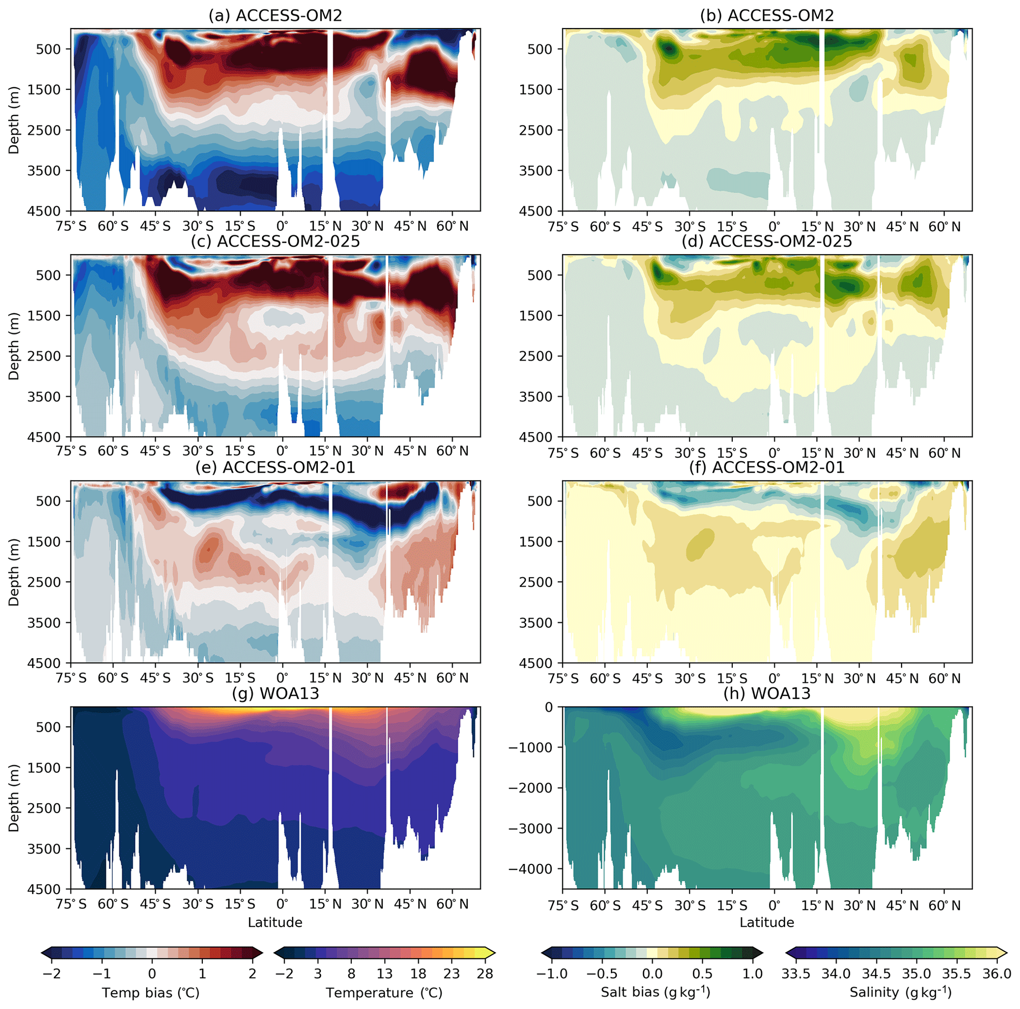
Figure 23Meridional transects of 1993–2017 mean potential temperature (left panels) and salinity (right panels) in the central Atlantic Ocean, along longitude 25∘ W, near the WOCE/GO-SHIP hydrographic line A16 for (a–b) ACCESS-OM2, (c–d) ACCESS-OM2-025, (e–f) ACCESS-OM2-01, and (g–h) gridded climatologies from WOA13 for the period 1985–2013.
The Brazil Current flows southward along the western boundary of the South Atlantic Ocean, separating at ∼40∘ S. The mean surface speed of this current in ACCESS-OM2-025 and ACCESS-OM2-01 is of comparable magnitude to, but weaker than, observations (Fig. 24b–d) and is strongly underestimated in ACCESS-OM2 (Fig. 24a). This underestimation is most clear for the upper 400 m of this current (not shown). Weakening of the Brazil Current is expected at the lowest resolution due to the broadening of the current by the enhanced viscosity near the western boundary. The Malvinas Current, flowing northwards along the boundary south of 40∘ S, is highly steered by bathymetry (Fig. 24d, h) and is well-represented in ACCESS-OM2-01 (Fig. 24c, g), including its northward penetration along the shelf break up to 40∘ S. The Brazil–Malvinas confluence mean latitude (∼38∘ S, Fig. 24d, h) is captured in ACCESS-OM2-01 but is too far south in ACCESS-OM2-025 and ACCESS-OM2. The Zapiola anticyclone (ZA) appears clearly at ∼42–48∘ S, ∼36–48∘ W in the Colin de Verdière and Ollitrault (2016) barotropic streamfunction (contours in Fig. 24h) but is weaker in ACCESS-OM2-01, indistinct in ACCESS-OM2-025, and absent in ACCESS-OM2 (Fig. 24g, f, e), consistent with the ZA being eddy-driven (Dewar, 1998; de Miranda et al., 1999); the poor representation at coarse resolution is associated with significant SST and SSS biases (Figs. 10 and 11). The sea level standard deviation forms a distinctive horseshoe pattern (Fu, 2006) around the ZA in the AVISO product (colours in Fig. 24h), which is partially captured in ACCESS-OM2-01, although at lower amplitude. The sea level variability pattern and amplitude in ACCESS-OM2-025 differ significantly from AVISO, and variability is negligible in ACCESS-OM2.
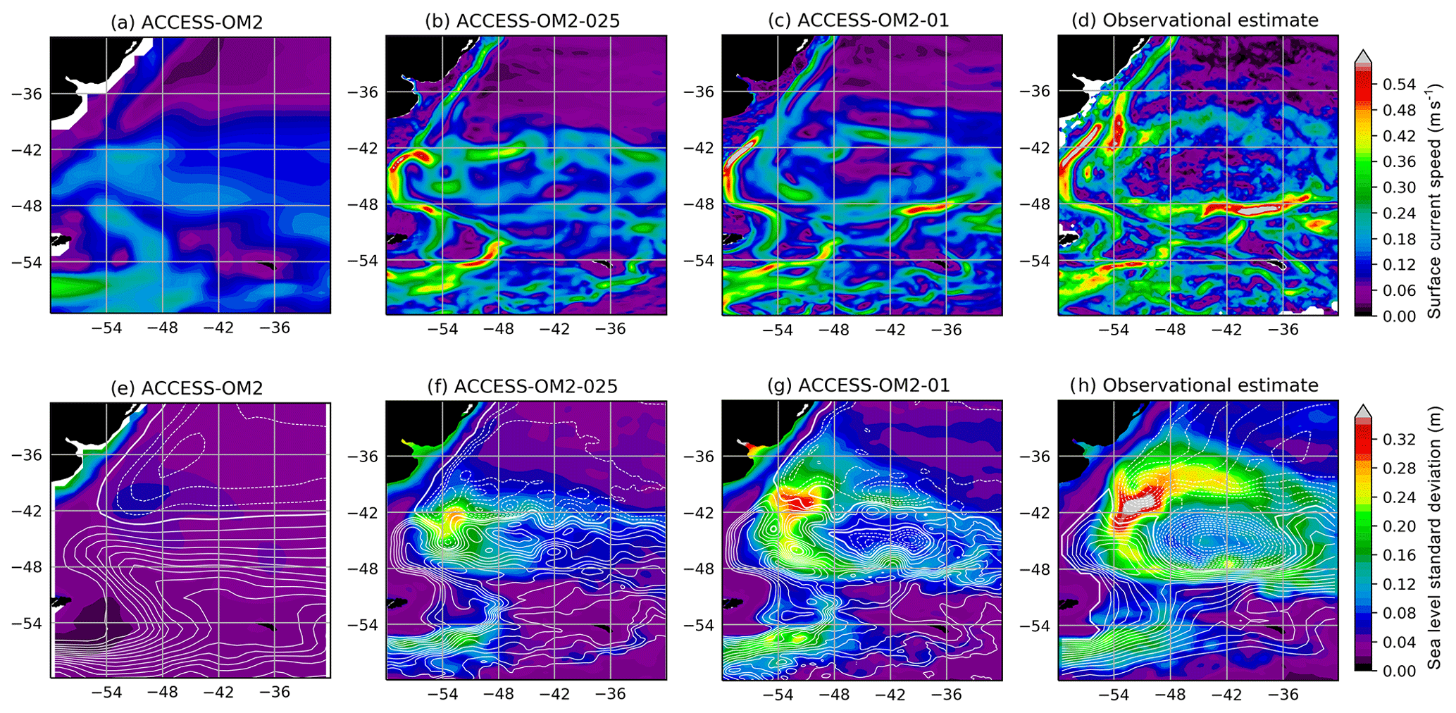
Figure 24Mean surface current speed in the southwest Atlantic in (a) ACCESS-OM2, (b) ACCESS-OM2-025, (c) ACCESS-OM2-01, and (d) estimated from drifter data (Laurindo et al., 2017). (e–h) Standard deviation of sea level anomaly (colours) and mean barotropic streamfunction (contours) as in Fig. 16 but with a different colour scale.
4.2.5 Indian Ocean
As in previous sections, we plot time-mean transects of potential temperature and salinity across the central Indian Ocean (longitude 95∘ E, near the I08–09 WOCE/GO-SHIP repeat hydrography line) from the three different model configurations, as well as from the WOA13 climatology, for the period 1985–2013. In the Indian Ocean, all three model configurations reproduce the basic structure of both temperature and salinity extremely well, including the high meridional temperature gradients near 50∘ S associated with the ACC, the low vertical temperature gradients near 40∘ S associated with the formation of mode and intermediate waters, the deep salinity minima in the Southern Hemisphere at a depth of around 1500 m, and the band of very fresh surface waters north of the Equator. The primary model biases are the cool water generated by convection near the southern boundary and a deep midlatitude thermocline in ACCESS-OM2 and ACCESS-OM2-025, while ACCESS-OM2-01 has minimal biases in this region.
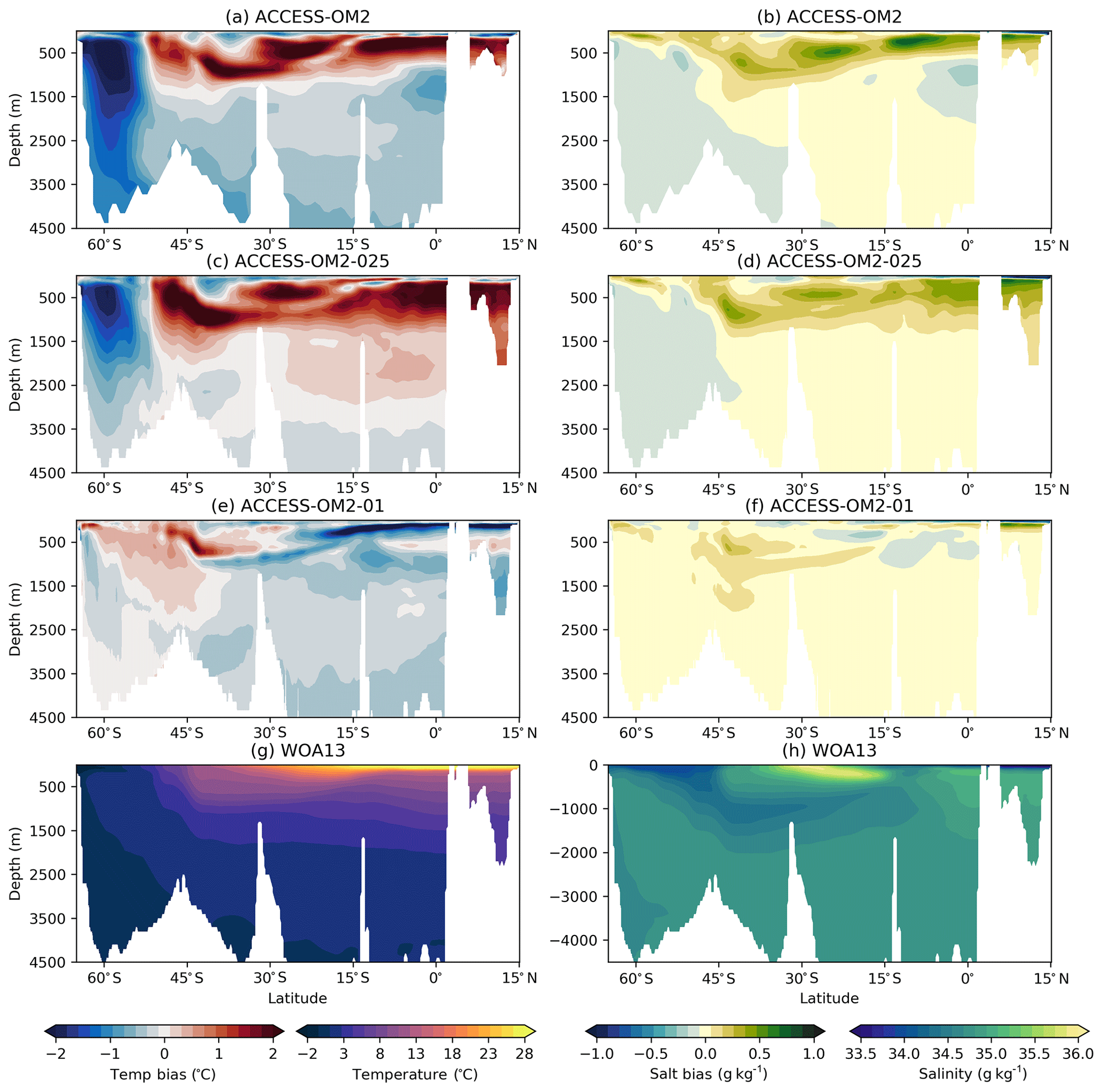
Figure 25Meridional transects of 1993–2017 mean potential temperature (upper panels) and salinity (lower panels) in the central Indian Ocean, along longitude 95∘ E, near the WOCE/GO-SHIP hydrographic lines I08 and I09 for (a–b) ACCESS-OM2, (c–d) ACCESS-OM2-025, (e–f) ACCESS-OM2-01, and (g–h) gridded climatologies from WOA13 for the period 1985–2013.
We also assess the annual and seasonal mean variability of the thermocline depth (D20) in the western tropical Indian Ocean (50–75∘ E, 5–10∘ S), known as the Seychelles Dome (Yokoi et al., 2008; Hermes and Reason, 2008), for 1985–2013 using the 20 ∘C isotherm proxy. All three model resolutions are able to simulate the basic large-scale annual mean D20 structure of the Indian Ocean (Fig. 26). In the coarse models (Fig. 26a, b), the D20 is deeper than observed (Fig. 26d) in four areas: the western Arabian Sea, the Seychelles Dome (black box), along the Mozambique Channel and across 15–25∘ S (particularly on the eastern side). The same model differences relative to WOA13 are evident over all seasons (not shown) for both the Seychelles Dome region and the large-scale Indian Ocean. Despite a general tendency to underestimate the D20 in ACCESS-OM2-01 within the tropical Indian Ocean (north of 10∘ S; Fig. 26c), the higher-resolution model compares best with the observed annual and seasonal spatial pattern in the Seychelles Dome region. This result suggests that higher-resolution ocean simulations are important to capture the Seychelles Dome thermocline variability and its role in regional weather and climate, from tropical cyclones (Xie et al., 2002) to rainfall in Africa (Annamalai et al., 2005; Behera et al., 2005), India (Izumo et al., 2008), and Australia (Taschetto et al., 2011).
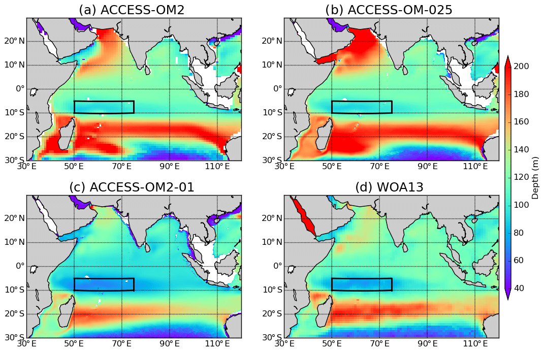
Figure 26Annual mean depth of the 20 ∘C isotherm (D20). (a) ACCESS-OM2; (b) ACCESS-OM2-025; (c) ACCESS-OM2-01; and (d) WOA13. The black box (50–75∘ E, 5–10∘ S) represents the position of the shallowest D20, which is used as a proxy for the thermocline ridge.
4.3 Sea ice
Our coupled ocean–ice model runs yield acceptable and very similar time series of Arctic and Antarctic sea ice extent and volume at all three horizontal resolutions (Fig. 27); however, there are some shortcomings when compared with observations. The final decades of our simulations cover a period of dramatic changes in sea ice (Fig. 27a, b): the Arctic sea ice underwent a drastic decline of the annual minimum extent (e.g. Stroeve et al., 2014), whereas the Antarctic annual maximum sea ice extent ramped up from 2012 to the maximum extent on record in 2014 before decreasing sharply from 2015 to the current (2019) minimum (e.g. Turner and Comiso, 2017). The Arctic sea ice decline during winter has been linked to an anomalous atmospheric circulation pattern bringing an increased inflow of warm air masses from lower latitudes and a general polar warming, while during summer the positive feedback (via the absorption of shortwave radiation and the resulting warming of the ocean mixed layer) contributes to the loss of summer sea ice in the Arctic (e.g. Stroeve and Notz, 2018). The interannual variability in the Antarctic sea ice extent has been attributed to a combination of thermodynamics (likely driven by increased glacial melt; Bintanja et al., 2015) and dynamics (e.g. Holland and Kwok, 2012; Schlosser et al., 2018). These observed interannual changes in sea ice extent are closely tracked by the ACCESS-OM2 suite at all resolutions in both hemispheres (Fig. 27a, b) and are also reflected in sea ice volume (Fig. 27c, d). The long-term trends in sea ice extent are also tracked by the 1 and 0.1∘ configurations, but the Arctic decline is slower than observed at 0.25∘ (Fig. 27a). Like CORE-II (Large and Yeager, 2009), the JRA-55 reanalysis (Kobayashi et al., 2015) incorporates observed sea ice concentration; however, JRA-55 treats regions with <55 % ice concentration as ice-free and regions exceeding this threshold as 100 % sea ice (unlike CORE-II, which combines ocean and ice fluxes in proportion to their concentration). We speculate that this hard ice edge causes a stronger imprint of the observed sea ice in the JRA55-do atmospheric state (e.g. reducing the 10 m air temperature over ice), which then drives the modelled ice concentration to a state resembling the observations. We now assess the quality of the spatial distribution of sea ice in the two hemispheres.
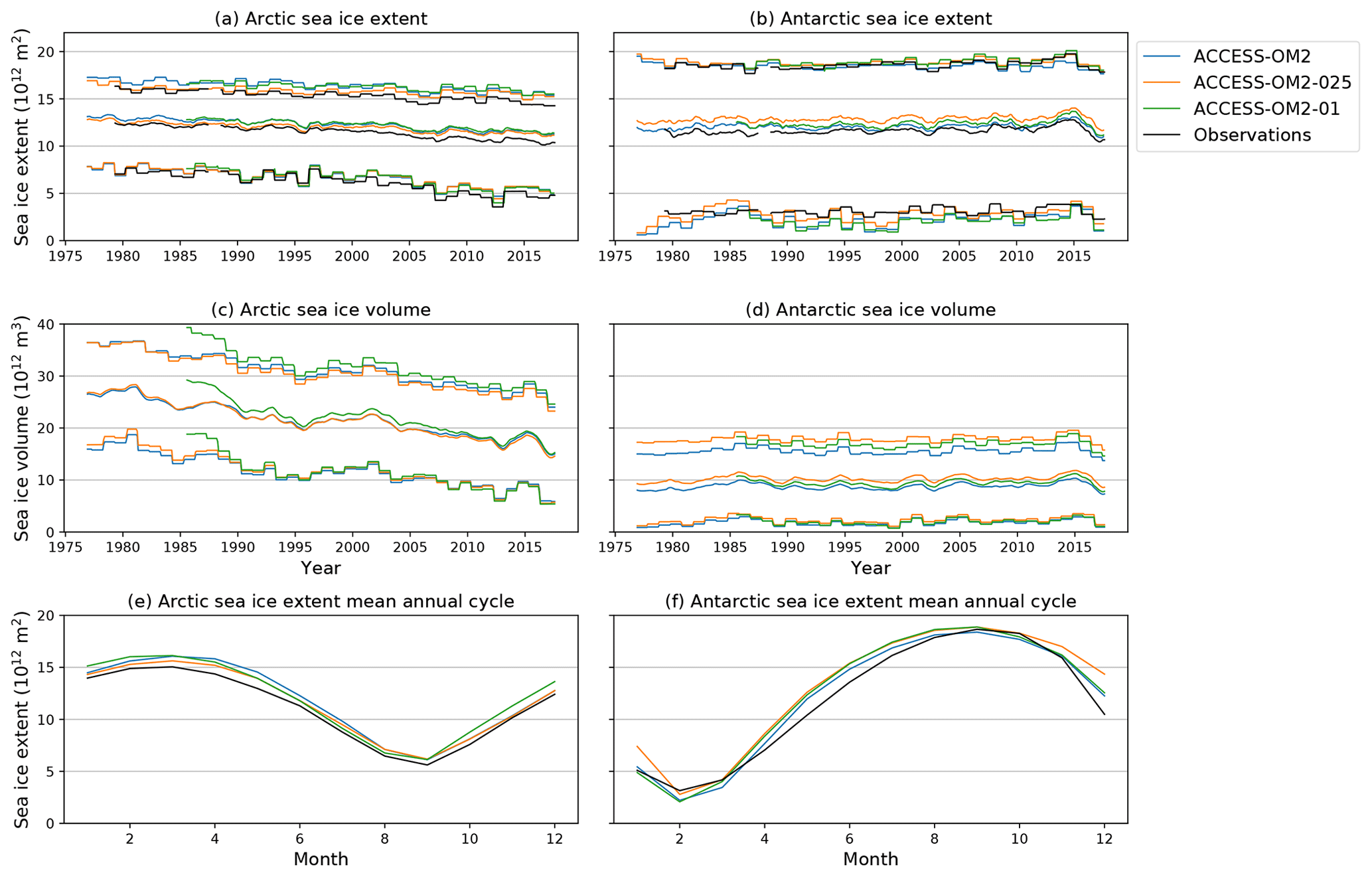
Figure 27(a–b) Sea ice extent, (c–d) volume, and (e–f) 1993–2017 mean annual cycle of the extent in the (a, c, e) Arctic and (b, d, f) Antarctic in the three configurations. Panels (a)–(d) show running 12-month minima, means, and maxima. Observational estimates are based on passive microwave retrievals (NSIDC Sea Ice Index version 3, Fetterer et al., 2017). Note that the three models and observations use different land masks, so the time series would not be expected to agree perfectly in magnitude.
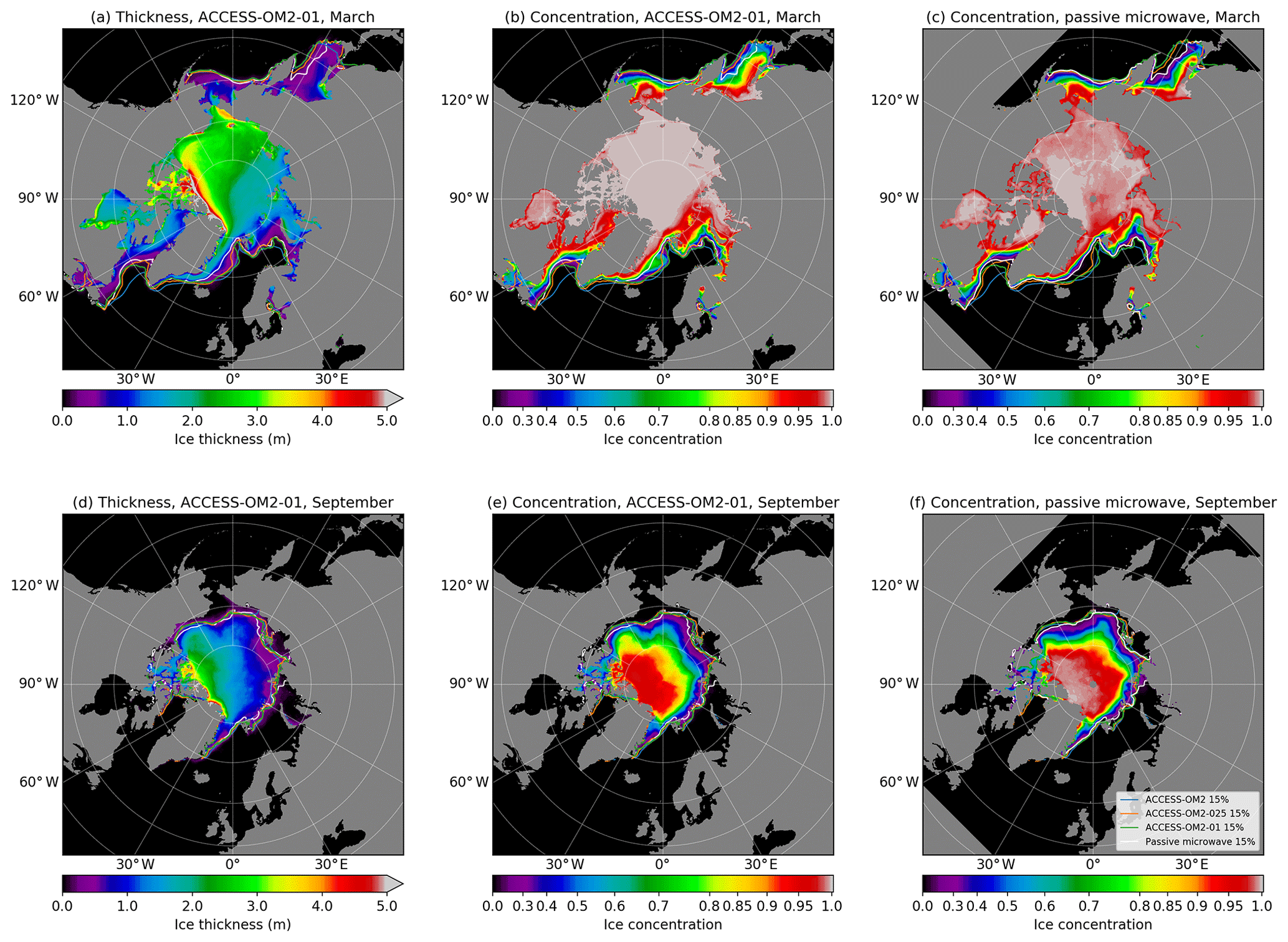
Figure 28The 1993–2017 mean Arctic sea ice thickness (ice volume per unit area; a, d) and concentration (ice area per unit area; b, e) in ACCESS-OM2-01 and concentration estimates from NOAA G02202 V3 passive microwave Goddard merged monthly data (Peng et al., 2013; Meier et al., 2017, c, f) for (a)–(c) March and (d)–(f) September. The concentration scale is nonlinear to highlight differences at high concentrations. Contour lines show the sea ice extent (defined as the 15 % concentration contour) in all three model configurations and observations.
4.3.1 Arctic Ocean
The Arctic sea ice biases in the ACCESS-OM suite appear considerably smaller than in most of the CORE-II-forced models investigated by Wang et al. (2016). The mean annual cycle of sea ice extent is close to the observed estimate (Fig. 27e) but seems to decline slightly too slowly in late spring. At all resolutions the simulated 1993–2017 monthly mean Arctic sea ice extent agrees well with observational estimates in most regions, as does the monthly mean concentration (contours and colour in Fig. 28b, c, e, f); however, some issues that warrant further investigation have been identified. At all resolutions the simulations exhibit a broad zone of sparse sea ice concentration in the eastern Sea of Okhotsk and southeast of Fram Strait at the March maximum, neither of which is observed (Fig. 28b, c). In ACCESS-OM2-01 the Canadian Archipelago, central Arctic, and Siberian coast exhibit a slightly excessive ice concentration during March, whereas in Baffin Bay the simulated ice concentration is low compared to observations. These biases are also present at coarser resolution, although the central Arctic bias is weaker (not shown). The ice extent in the Labrador Sea is also excessive in March at 1∘. At the September minimum the ice extent closely matches observations (apart from some excess coverage in eastern Siberia), but the overall concentration is slightly too low in ACCESS-OM2-01 (Fig. 28e, f) and in the coarser resolutions (not shown). In broad agreement with results from the Pan-Arctic Ice Ocean Model and Assimilation System (PIOMAS; Zhang and Rothrock, 2003), the thickest ice in our runs is found close to the Canadian Archipelago (Fig. 28a, d). However, rather than being transported northward through the Beaufort Gyre and eventually out of the central Arctic via the transpolar drift, much of the sea ice in our simulation remains within the Canadian Arctic. Investigation of the causes of these biases is beyond the scope of this paper, but possible contributing factors include SST biases (Fig. 10), issues regarding the modelled mixed layer depth, and bias in the 0.1∘ initial condition.
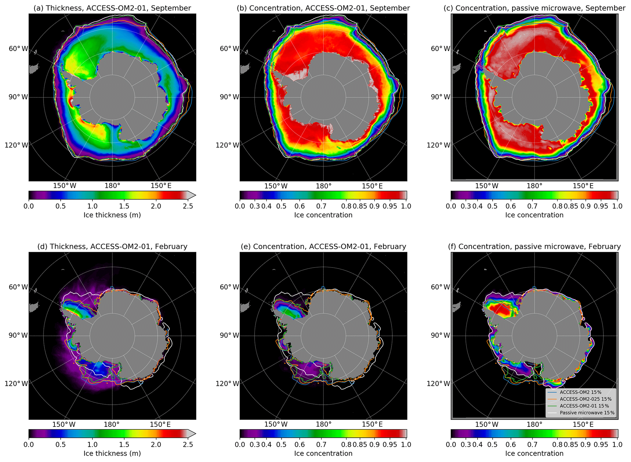
Figure 29As for Fig. 28 but in the Antarctic for (a)–(c) September and (d)–(f) February.
Finally, we note that the sea ice in the 0.1∘ simulation displays many long, narrow, linear zones of low ice concentration and high strain rate (not shown) which open and close on timescales of days, largely in response to varying wind stress. These lead-like linear kinematic features are too narrow to resolve with existing satellite passive microwave instruments (Lemieux et al., 2015) and are characteristic of high-resolution models with EVP rheology (e.g. Hutchings et al., 2005) as a result of strain localization. While their spatiotemporal scaling may only be partially correct at this resolution (Hutter et al., 2018), we consider the presence of these lead-like features to be an improvement over the very smooth fields obtained in coarser EVP models. Linear kinematic features are also evident in the Antarctic ice but are less ubiquitous than in the Arctic.
4.3.2 Southern Hemisphere
At all resolutions the modelled 1993–2017 mean annual cycle of Antarctic sea ice extent closely matches observational estimates, although ice growth appears to occur slightly more rapidly than observed (Fig. 27f). The spatial structure of the modelled 1993–2017 mean Antarctic spring maximum sea ice extent agrees well with that derived from passive microwave observations at all resolutions and is particularly realistic in the 0.1∘ simulation (contours in Fig. 29b, c). During Antarctic winter and early spring the simulated sea ice concentration is too high near the coast at 0.1∘ and a fraction too low in the wider pack-ice zone (Fig. 29b, c); at coarser resolutions the concentration becomes smaller in both regions, reducing the positive bias near the coast but increasing the negative bias in the outer pack (not shown). We note that the high-concentration coastal ice in the model is very thin (Fig. 29a), with most of the ice cover in the thinnest thickness category (<0.64 m; not shown) and high frazil production (not shown), consistent with the presence of newly forming sea ice in coastal polynyas. Passive microwave products are known to underestimate the concentration of thin ice, such as in polynyas or marginal ice zones during autumn and winter (e.g. Meier et al., 2014; Ivanova et al., 2015), suggesting that the discrepancy with the model may be partly due to a bias in the observational estimate.
The simulated annual minimum sea ice extent is much too low in the Weddell Sea and most of East Antarctica, and too high in the Ross Sea, at all three resolutions (contours in Fig. 29e, f). This is associated with low concentrations at all resolutions in all regions other than the northern Ross Sea; this bias is also typical of a wide variety of models driven by CORE-II forcing (Downes et al., 2015). The thickness distribution also reveals broad regions of very low-concentration sea ice extending well beyond the model's 15 % concentration contour (Fig. 29d). This ice is mostly in the thickest two categories (>2.47 m), i.e. second-year ice. Sea ice concentration builds up rapidly from its low minimum, reaching realistically high values in the outer pack by May–June, but the concentration then declines early relative to microwave observations, apparently preconditioning the ice for an overly rapid melt rate towards its overly low minimum. Further investigation is needed to understand the interplay between the oceanic mixed layer and associated SST and SSS biases, ice advection and thickness, and sea ice growth or melt processes, but this is beyond the scope of this paper.
The ACCESS-OM2 model suite is specifically designed as a model hierarchy, with supported configurations at three different horizontal resolutions. The model configurations are highly consistent (largely “traceable” in the terminology of Storkey et al., 2018); this feature makes the model suite ideal for studies investigating the sensitivity of solutions to model resolution. This hierarchy is also advantageous for model improvement at all resolutions. For example, when building or testing new configurations, these tests can first be done at low resolution, confirming basic conservation properties before proceeding to more expensive, high-resolution cases. It is also designed to lead to a convergence of operational uses of the model, with high-resolution ocean prediction systems able to align with the code base used for coupled simulations.
This paper has outlined the development of this model and in particular documented the new features of this model and the coupling between its components. It has also enabled a moderately thorough evaluation of ACCESS-OM2 at each resolution, with the goal of providing information on which aspects of the model can be used for different research or operational objectives. This approach also has the benefit of providing a benchmark for future developments.
In general terms, the model does a good job of representing many features of the ocean, particularly at high resolution. Historical sea ice extent trends are well-represented, and the surface properties and transects in each ocean basin compare well with the observational record. The large-scale overturning circulation, flow through the Indonesian archipelago, and patterns of boundary currents are generally realistic, supporting the notion that this suite of models is competitive with similar models from other institutions. Areas for improvement include the Gulf Stream behaviour and associated North Atlantic SST and SSS biases, the weaker than observed Drake Passage transport, and the weak AMOC in the 1∘ configuration. In addition, more work is needed to understand differences between observed and modelled meridional heat transport.
One feature of the model evaluation exercise was to highlight a general improvement of many model metrics at higher resolution. In particular, Southern Ocean water masses, the Antarctic shelf region, the overturning circulation, and the western boundary current regions are all much improved in ACCESS-OM2-01 compared with the coarser resolutions. However, the highest-resolution model also has the weakest Antarctic Circumpolar Current transport, has an overly strong equatorial Pacific thermocline, and continues to have biases in western boundary current regions despite the high resolution. These features will continue to be investigated. To what extent these resolution-dependent changes are related to changes in model dynamics or to differing error cancellation with forcing biases remains an open question.
A feature of modern model development is the continuous and collaborative process of building software. A version of ACCESS-OM2 has been frozen to enable other users to replicate these simulations (see the “Code availability” section below) but it will be continuously developed. These incremental improvements will be publicly available via the model GitHub site, allowing users to both adopt and contribute to the future evolution of the model.
The ACCESS-OM2 source code and configurations used for the simulations in this paper are available from https://doi.org/10.5281/zenodo.2653246 (Hannah et al., 2019). The ACCESS-OM2 code is undergoing continuous development, and these developments (including the MOM5 and CICE5 distributions) are publicly available at https://github.com/COSIMA/access-om2 (last access: 21 January 2020). All model components (MOM5, CICE5, OASIS3-MCT, YAML, and libaccessom2) are open-source. The model output for the simulations presented in this paper will be stored on the COSIMA data collection, available from https://doi.org/10.4225/41/5a2dc8543105a (COSIMA, 2019).
The supplement related to this article is available online at: https://doi.org/10.5194/gmd-13-401-2020-supplement.
This paper is a broad collaboration between a number of institutions. The technical side of the project was led by NH, with substantial contributions from MLW, RF, and AH, as well as many other contributions from the community. The model simulations were conducted primarily by AEK, AMcH, and AS. Analysis of the output and the writing of text for the paper represented a broad effort coordinated by Hogg and Kiss with substantial contributions from FBD, MAC, CC, ERD, PH, RMH, AMcH, AEK, AK, GSP, OR, AS, PS, MLW, and XZ.
The authors declare that they have no conflict of interest.
This paper is the first significant research publication from the Consortium for Ocean–Sea Ice Modelling in Australia (COSIMA; http://cosima.org.au, last access: 21 January 2020), which is funded by the Australian Research Council (ARC) through its Linkage Program (LP160100073). This research was supported by the ARC Centre of Excellence for Climate Extremes, which is supported by the ARC via grant CE170100023. This research was undertaken with the assistance of resources from the National Computational Infrastructure, which is supported by the Australian Government. Océane Richet was supported by the Centre for Southern Hemisphere Oceans Research. Fabio Boeira Dias, Catia M. Domingues, Petra Heil, Andreas Klocker, Simon J. Marsland, and Abhishek Savita were supported by the Australian Government's Cooperative Research Centres Programme through the Antarctic Climate and Ecosystems Cooperative Research Centre. The International Space Science Institute (Bern, Switzerland) is thanked for supporting scientific collaborations in this study through project 406. This work contributes to the Australian Antarctic Science projects 4301 and 4390. Simon J. Marsland and Peter Dobrohotoff are supported by the Earth Systems and Climate Change Hub of the Australian Government's National Environmental Science Program. Catia M. Domingues was supported by the ARC (FT13101532 and DP160103130). Adele K. Morrison was supported by an ARC DECRA Fellowship DE170100184. This study used SSALTO/DUACS SLA produced and distributed by the Copernicus Marine Environment Monitoring Service (http://marine.copernicus.eu, last access: 21 January 2020) and MDT_CNES-CLS produced by CLS and distributed by AVISO+, with support from CNES (https://www.aviso.altimetry.fr, last access: 21 January 2020). Our thanks to Alain Colin de Verdière, who provided barotropic streamfunction data for model comparisons. We thank Pat Hyder (UKMO) and the anonymous referee for their insightful and constructive comments, which have improved this paper.
This research has been supported by the Australian Research Council (grant nos. LP160100073, CE170100023, FT13101532, DP160103130 and DE170100184), the International Space Science Institute (grant no. 406), and the Australian Antarctic Science (grant nos. 4301 and 4390).
This paper was edited by Robert Marsh and reviewed by P. Hyder and one anonymous referee.
Adcroft, A. and Campin, J.-M.: Rescaled height coordinates for accurate representation of free-surface flows in ocean circulation models, Ocean Modell., 7, 269–284, 2004. a
Adcroft, A., Hill, C., and Marshall, J.: Representation of topography by shaved cells in a height coordinate ocean model, Mon. Weather Rev., 125, 2293–2315, 1997. a, b
Annamalai, H., Liu, P., and Xie, S. P.: Southwest Indian Ocean SST variability: Its local effect and remote influence on Asian monsoons, J. Climate, 18, 4150–4167, https://doi.org/10.1175/JCLI3533.1, 2005. a
Ansorge, I. J., Froneman, P. W., and Durgadoo, J. V.: The Marine Ecosystem of the Sub-Antarctic, Prince Edward Islands, in: Marine Ecosystems, edited by: Cruzado, A., chap. 3, IntechOpen, Rijeka, https://doi.org/10.5772/36676, 2012. a
Bamber, J., van den Broeke, M., Ettema, J., Lenaerts, J., and Rignot, E.: Recent large increases in freshwater fluxes from Greenland into the North Atlantic, Geophys. Res. Lett., 39, L19501, https://doi.org/10.1029/2012gl052552, 2012. a
Barnier, B., Blaker, A., Biastoch, A., Böning, C., Coward, A., Deshayes, J., Hirshi, J., Le Sommer, J., Madec, G., Maze, G., Molines, J., New, A., Penduff, T., Scheinert, M., Talandier, C., and Treguier, A.-M.: DRAKKAR: developing high resolution ocean components for European Earth system models, CLIVAR Exch., 19, 18–21, 2014. a
Beckmann, A. and Döscher, R.: A Method for Improved Representation of Dense Water Spreading over Topography in Geopotential-Coordinate Models, J. Phys. Oceanogr., 27, 581–591, https://doi.org/10.1175/1520-0485(1997)027<0581:amfiro>2.0.co;2, 1997. a
Behera, K. S., Luo, J.-J., Masson, S., Delecluse, P., Gualdi, S., Navarra, A., and Toshio, Y.: Paramount Impact of the Indian Ocean Dipole on the East African Short Rains : A CGCM Study, J. Climate, 18, 4514–4530, 2005. a
Bentley, J. L.: Multidimensional Binary Search Trees Used for Associative Searching, Commun. ACM, 18, 509–517, https://doi.org/10.1145/361002.361007, 1975. a
Bi, D. and Marsland, S.: Australian Climate Ocean Model (AusCOM) users guide, CAWCR Technical Report 27, The Centre for Australian Weather and Climate Research, available at: http://www.cawcr.gov.au/technical-reports/CTR_027.pdf (last access: 21 January 2020), 2010. a
Bi, D., Dix, M., Marsland, S. J., O'Farrell, S., Rashid, H. A., Uotila, P., Hirst, A. C., Kowalczyk, E., Golebiewski, M., Sullivan, A., Yan, H., Hannah, N., Franklin, C., Sun, Z., Vohralik, P., Watterson, I., Zhou, X., Fiedler, R., Collier, M., Ma2, Y., Noonan, J., Stevens, L., Uhe, P., Zhu, H., Griffies, S. M., Hill, R., Harris, C., and Puri, K.: The ACCESS coupled model: description, control climate and evaluation, Aust. Met. Ocean. J., 63, 61–64, 2013a. a
Bi, D., Marsland, S., Uotila, P., O'Farrell, S., Fiedler, R., Sullivan, A., Griffies, S., Zhou, X., and Hirst, A.: ACCESS-OM: the ocean and sea-ice core of the ACCESS coupled model, Aust. Meteorol. Oceanogr. J., 63, 213–232, 2013b. a, b, c, d, e, f, g, h, i, j, k, l, m, n
Bintanja, R., van Oldenborgh, G., and Katsman, C.: The effect of increased fresh water from Antarctic ice shelves on future trends in Antarctic sea ice, Ann. Glaciol., 56, 120–126, https://doi.org/10.3189/2015aog69a001, 2015. a
Bishop, S. P., Gent, P. R., Bryan, F. O., Thompson, A. F., Long, M. C., and Abernathey, R.: Southern Ocean Overturning Compensation in an Eddy-Resolving Climate Simulation, J. Phys. Oceanogr., 46, 1575–1592, https://doi.org/10.1175/JPO-D-15-0177.1, 2016. a
Bitz, C. M. and Lipscomb, W. H.: An energy-conserving thermodynamic model of sea ice, J. Geophys. Res.-Oceans, 104, 15669–15677, https://doi.org/10.1029/1999jc900100, 1999. a
Bryan, F., Hecht, M., and Smith, R.: Resolution convergence and sensitivity studies with North Atlantic circulation models. Part 1: The western boundary current system, Ocean Modell., 16, 141–159, 2007. a, b
Campin, J.-M. and Goosse, H.: Parameterization of density-driven downsloping flow for a coarse-resolution ocean model in z-coordinate, Tellus A: Dynam. Meteorol. Oceanogr., 51, 412–430, https://doi.org/10.3402/tellusa.v51i3.13468, 1999. a
Chambers, D. P.: Using kinetic energy measurements from altimetry to detect shifts in the positions of fronts in the Southern Ocean, Ocean Sci., 14, 105–116, https://doi.org/10.5194/os-14-105-2018, 2018. a
Chassignet, W. and Marshall, D.: Gulf Stream separation in numerical ocean models, Geophys. Monogr. Ser., 177, 39–61, 2008. a
Colella, P. and Woodward, P. R.: The Piecewise Parabolic Method (PPM) for gas-dynamical simulations, J. Comput. Phys., 54, 174–201, https://doi.org/10.1016/0021-9991(84)90143-8, 1984. a
Colin de Verdière, A. and Ollitrault, M.: A Direct Determination of the World Ocean Barotropic Circulation, J. Phys. Oceanogr., 46, 255–273, https://doi.org/10.1175/jpo-d-15-0046.1, 2016. a, b
COSIMA: COSIMA Model Output Collection, available at: https://doi.org/10.4225/41/5a2dc8543105a (last access: 21 January 2020), 2019.
Craig, A. P., Mickelson, S. A., Hunke, E. C., and Bailey, D. A.: Improved parallel performance of the CICE model in CESM1, Int. J. High Perform. Comput. Appl., 29, 154–165, https://doi.org/10.1177/1094342014548771, 2015. a, b
Danabasoglu, G., Yeager, S. G., Bailey, D., Behrens, E., Bentsen, M., Bi, D., Biastoch, A., Böning, C., Bozec, A., Canuto, V. M., Cassou, C., Chassignet, E., Coward, A. C., Danilov, S., Diansky, N., Drange, H., Farneti, R., Fernandez, E., Fogli, P. G., Forget, G., Fujii, Y., Griffies, S. M., Gusev, A., Heimbach, P., Howard, A., Jung, T., Kelley, M., Large, W. G., Leboissetier, A., Lu, J., Madec, G., Marsland, S. J., Masina, S., Navarra, A., Nurser, A. G., Pirani, A., Salas y Mélia, D., Samuels, B. L., Scheinert, M., Sidorenko, D., Treguier, A.-M., Tsujino, H., Uotila, P., Valcke, S., Voldoire, A., and Wang, Q.: North Atlantic Simulations in Coordinated Ocean-ice Reference Experiments phase II (CORE-II). Part 1: Mean States, Ocean Modell., 73, 76–107, https://doi.org/10.1016/j.ocemod.2013.10.005, 2014. a, b, c, d
Delworth, T. L., Rosati, A., Anderson, W., Adcroft, A. J., Balaji, V., Benson, R., Dixon, K., Griffies, S. M., Lee, H.-C., Pacanowski, R. C., Vecchi, G. A., Wittenberg, A. T., Zeng, F., and Zhang, R.: Simulated Climate and Climate Change in the GFDL CM2.5 High-Resolution Coupled Climate Model, J. Climate, 25, 2755–2781, https://doi.org/10.1175/jcli-d-11-00316.1, 2012. a
de Miranda, A. P., Barnier, B., and Dewar, W. K.: On the dynamics of the Zapiola Anticyclone, J. Geophys. Res.-Oceans, 104, 21137–21149, https://doi.org/10.1029/1999JC900042, 1999. a
de Ruijter, W. P. M., Ridderinkhof, H., Lutjeharms, J. R. E., Schouten, M. W., and Veth, C.: Observations of the flow in the Mozambique Channel, Geophys. Res. Lett., 29, 1502, https://doi.org/10.1029/2001GL013714, 2002. a
Dencausse, G., Arhan, M., and Speich, S.: Routes of Agulhas rings in the southeastern Cape Basin, Deep Sea Res. Part I, 57, 1406–1421, https://doi.org/10.1016/j.dsr.2010.07.008, 2010. a
Depoorter, M. A., Bamber, J. L., Griggs, J. A., Lenaerts, J. T. M., Ligtenberg, S. R. M., van den Broeke, M. R., and Moholdt, G.: Calving fluxes and basal melt rates of Antarctic ice shelves, Nature, 502, 89–92, https://doi.org/10.1038/nature12567, 2013. a, b
Dewar, W. K.: Topography and barotropic transport control by bottom friction, J. Mar. Res., 56, 295–328, https://doi.org/10.1357/002224098321822320, 1998. a
Donohue, K. A., Tracey, K. L., Watts, D. R., Chidichimo, M. P., and Chereskin, T. K.: Mean Antarctic Circumpolar Current transport measured in Drake Passage, Geophys. Res. Lett., 43, 11760–11767, https://doi.org/10.1002/2016GL070319, 2016. a, b
Döscher, R. and Beckmann, A.: Effects of a Bottom Boundary Layer Parameterization in a Coarse-Resolution Model of the North Atlantic Ocean, J. Atmos. Ocean. Technol., 17, 698–707, https://doi.org/10.1175/1520-0426(2000)017<0698:eoabbl>2.0.co;2, 2000. a
Downes, S. M., Farneti, R., Uotila, P., Griffies, S. M., Marsland, S. J., Bailey, D., Behrens, E., Bentsen, M., Bi, D., Biastoch, A., Böning, C., Bozec, A., Canuto, V. M., Chassignet, E., Danabasoglu, G., Danilov, S., Diansky, N., Drange, H., Fogli, P. G., Gusev, A., Howard, A., Ilicak, M., Jung, T., Kelley, M., Large, W. G., Leboissetier, A., Long, M., Lu, J., Masina, S., Mishra, A., Navarra, A., Nurser, A. G., Patara, L., Samuels, B. L., Sidorenko, D., Spence, P., Tsujino, H., Wang, Q., and Yeager, S. G.: An assessment of Southern Ocean water masses and sea ice during 1988-2007 in a suite of interannual CORE-II simulations, Ocean Modell., 94, 67–94, https://doi.org/10.1016/j.ocemod.2015.07.022, 2015. a
Dufour, C. O., Morrison, A. K., Griffies, S. M., Frenger, I., Zanowski, H., and Winton, M.: Preconditioning of the Weddell Sea Polynya by the Ocean Mesoscale and Dense Water Overflows, J. Clim., 30, 7719–7737, https://doi.org/10.1175/jcli-d-16-0586.1, 2017. a
Dufresne, J.-L., Foujols, M.-A., Denvil, S., Caubel, A., Marti, O., Aumont, O., Balkanski, Y., Bekki, S., Bellenger, H., Benshila, R., Bony, S., Bopp, L., Braconnot, P., Brockmann, P., Cadule, P., Cheruy, F., Codron, F., Cozic, A., Cugnet, D., de Noblet, N., Duvel, J.-P., Ethé, C., Fairhead, L., Fichefet, T., Flavoni, S., Friedlingstein, P., Grandpeix, J.-Y., Guez, L., Guilyardi, E., Hauglustaine, D., Hourdin, F., Idelkadi, A., Ghattas, J., Joussaume, S., Kageyama, M., Krinner, G., Labetoulle, S., Lahellec, A., Lefebvre, M.-P., Lefevre, F., Levy, C., Li, Z. X., Lloyd, J., Lott, F., Madec, G., Mancip, M., Marchand, M., Masson, S., Meurdesoif, Y., Mignot, J., Musat, I., Parouty, S., Polcher, J., Rio, C., Schulz, M., Swingedouw, D., Szopa, S., Talandier, C., Terray, P., Viovy, N., and Vuichard, N.: Climate change projections using the IPSL-CM5 Earth System Model: from CMIP3 to CMIP5, Clim. Dynam., 40, 2123–2165, https://doi.org/10.1007/s00382-012-1636-1, 2013. a
Dukowicz, J. K. and Baumgardner, J. R.: Incremental Remapping as a Transport/Advection Algorithm, J. Comput. Phys., 160, 318–335, https://doi.org/10.1006/jcph.2000.6465, 2000. a
Farneti, R., Downes, S. M., Griffies, S. M., Marsland, S. J., Behrens, E., Bentsen, M., Bi, D., Biastoch, A., Böning, C., Bozec, A., Canuto, V. M., Chassignet, E., Danabasoglu, G., Danilov, S., Diansky, N., Drange, H., Fogli, P. G., Gusev, A., Hallberg, R. W., Howard, A., Ilicak, M., Jung, T., Kelley, M., Large, W. G., Leboissetier, A., Long, M., Lu, J., Masina, S., Mishra, A., Navarra, A., George Nurser, A. J., Patara, L., Samuels, B. L., Sidorenko, D., Tsujino, H., Uotila, P., Wang, Q., and Yeager, S. G.: An assessment of Antarctic Circumpolar Current and Southern Ocean meridional overturning circulation during 1958-2007 in a suite of interannual CORE-II simulations, Ocean Modell., 93, 84–120, https://doi.org/10.1016/j.ocemod.2015.07.009, 2015. a
Ferrari, R., Griffies, S. M., Nurser, A. G., and Vallis, G. K.: A boundary-value problem for the parameterized mesoscale eddy transport, Ocean Modell., 32, 143–156, https://doi.org/10.1016/j.ocemod.2010.01.004, 2010. a
Fetterer, F., Knowles, K., Meier, W., Savoie, M., and Windnagel, A. K.: Sea Ice Index, Version 3, Tech. rep., NSIDC: National Snow and Ice Data Center, Boulder, Colorado, USA, https://doi.org/10.7265/N5K072F8, 2017, updated daily. a
Fox-Kemper, B., Ferrari, R., and Hallberg, R.: Parameterization of mixed layer eddies. Part I: Theory and diagnosis, J. Phys. Oceanogr., 38, 1145–1165, https://doi.org/10.1175/2007JPO3792.1, 2008. a
Fu, L. L.: Pathways of eddies in the South Atlantic Ocean revealed from satellite altimeter observations, Geophys. Res. Lett., 33, 1–5, https://doi.org/10.1029/2006GL026245, 2006. a
Ganachaud, A. and Wunsch, C.: Large-Scale Ocean Heat and Freshwater Transports during the World Ocean Circulation Experiment, J. Climate, 16, 696–705, https://doi.org/10.1175/1520-0442(2003)016<0696:LSOHAF>2.0.CO;2, 2003. a, b
GEBCO: The GEBCO_2014 Grid, available at: https://www.gebco.net/ (last access: 21 January 2020), 2014. a
Gent, P. R. and McWilliams, J. C.: Isopycnal Mixing in Ocean Circulation Models, J. Phys. Oceanogr., 20, 150–155, https://doi.org/10.1175/1520-0485(1990)020<0150:IMIOCM>2.0.CO;2, 1990. a, b
Griffies, S. and Hallberg, R.: Biharmonic friction with a Smagorinsky-like viscosity for use in large-scale eddy-permitting ocean models, Mon. Weather Rev., 128, 2935–2946, 2000. a
Griffies, S. M.: The Gent-McWilliams Skew Flux, J. Phys. Oceanogr., 28, 831–841, https://doi.org/10.1175/1520-0485(1998)028<0831:TGMSF>2.0.CO;2, 1998. a
Griffies, S. M.: Elements of the Modular Ocean Model (MOM) 5 (2012 release with updates), Technical Report 7, NOAA/Geophysical Fluid Dynamics Laboratory Ocean Group, 2012. a, b, c, d
Griffies, S. M., Gnanadesikan, A., Pacanowski, R. C., Larichev, V. D., Dukowicz, J. K., and Smith, R. D.: Isoneutral Diffusion in a z-Coordinate Ocean Model, J. Phys. Oceanogr., 28, 805–830, https://doi.org/10.1175/1520-0485(1998)028<0805:IDIAZC>2.0.CO;2, 1998. a, b
Griffies, S. M., Gnanadesikan, A., Dixon, K. W., Dunne, J. P., Gerdes, R., Harrison, M. J., Rosati, A., Russell, J. L., Samuels, B. L., Spelman, M. J., Winton, W., and Zhang, R.: Formulation of an ocean model for global climate simulations, Ocean Sci., 1, 45–79, https://doi.org/10.5194/os-1-45-2005, 2005. a, b, c
Griffies, S. M., Biastoch, A., Böning, C. W., Bryan, F., Danabasoglu, G., Chassignet, E., England, M. H., Gerdes, R., Haak, H., Hallberg, R. W., Hazeleger, W., Jungclaus, J., Large, W. G., Madec, G., Pirani, A., Samuels, B. L., Scheinert, M., Sen Gupta, A., Severijns, C. A., Simmons, H. L., Treguier, A. M., Winton, M., Yeager, S., and Yin, J.: Coordinated Ocean-ice Reference Experiments (COREs), Ocean Modell., 26, 1–46, https://doi.org/10.1016/j.ocemod.2008.08.007, 2009. a, b, c, d, e, f
Griffies, S. M., Yin, J., Durack, P. J., Goddard, P., Bates, S. C., Behrens, E., Bentsen, M., Bi, D., Biastoch, A., Böning, C. W., Bozec, A., Chassignet, E., Danabasoglu, G., Danilov, S., Domingues, C. M., Drange, H., Farneti, R., Fernandez, E., Greatbatch, R. J., Holland, D. M., Ilicak, M., Large, W. G., Lorbacher, K., Lu, J., Marsland, S. J., Mishra, A., Nurser, A. G., Salas y Mélia, D., Palter, J. B., Samuels, B. L., Schröter, J., Schwarzkopf, F. U., Sidorenko, D., Treguier, A. M., Tseng, Y.-H., Tsujino, H., Uotila, P., Valcke, S., Voldoire, A., Wang, Q., Winton, M., and Zhang, X.: An assessment of global and regional sea level for years 1993–2007 in a suite of interannual CORE-II simulations, Ocean Modell., 78, 35–89, https://doi.org/10.1016/j.ocemod.2014.03.004, 2014. a, b
Griffies, S. M., Winton, M., Anderson, W. G., Benson, R., Delworth, T. L., Dufour, C. O., Dunne, J. P., Goddard, P., Morrison, A. K., Rosati, A., Wittenberg, A. T., Yin, J., and Zhang, R.: Impacts on Ocean Heat from Transient Mesoscale Eddies in a Hierarchy of Climate Models, J. Climate, 28, 952–977, 2015. a, b, c, d, e, f, g
Griffies, S. M., Danabasoglu, G., Durack, P. J., Adcroft, A. J., Balaji, V., Böning, C. W., Chassignet, E. P., Curchitser, E., Deshayes, J., Drange, H., Fox-Kemper, B., Gleckler, P. J., Gregory, J. M., Haak, H., Hallberg, R. W., Heimbach, P., Hewitt, H. T., Holland, D. M., Ilyina, T., Jungclaus, J. H., Komuro, Y., Krasting, J. P., Large, W. G., Marsland, S. J., Masina, S., McDougall, T. J., Nurser, A. J. G., Orr, J. C., Pirani, A., Qiao, F., Stouffer, R. J., Taylor, K. E., Treguier, A. M., Tsujino, H., Uotila, P., Valdivieso, M., Wang, Q., Winton, M., and Yeager, S. G.: OMIP contribution to CMIP6: experimental and diagnostic protocol for the physical component of the Ocean Model Intercomparison Project, Geosci. Model Dev., 9, 3231–3296, https://doi.org/10.5194/gmd-9-3231-2016, 2016. a
Haidvogel, D., McWilliams, J., and Gent, P.: Boundary current separation in a quasigeostrophic, eddy-resolving ocean circulation model, J. Phys. Oceanogr., 22, 882–902, 1992. a
Hallberg, R.: Using a resolution function to regulate parameterizations of oceanic mesoscale eddy effects, Ocean Modell., 72, 92–103, https://doi.org/10.1016/j.ocemod.2013.08.007, 2013. a, b
Hallberg, R.: Numerical instabilities of the ice/ocean coupled system, CLIVAR Exchanges, 65, 38–42, available at: http://www.clivar.org/sites/default/files/documents/exchanges65_0.pdf (last access: 21 January 2020), 2014. a
Han, W., Meehl, G. A., Stammer, D., Hu, A., Hamlington, B., Kenigson, J., Palanisamy, H., and Thompson, P.: Spatial Patterns of Sea Level Variability Associated with Natural Internal Climate Modes, Surv. Geophys., 38, 217–250, https://doi.org/10.1007/s10712-016-9386-y, 2017. a
Hannah, N., Kiss, A. E., Heerdegen, A., Ward, M. L., Fiedler, R., Hogg, A. M., Griffies, S. M., and Holmes, R. M.: The ACCESS-OM2 global ocean – sea ice coupled model (version 1.0), Zenodo, https://doi.org/10.5281/zenodo.2653246, 2019. a
Hermes, J. C. and Reason, C. J. C.: Annual cycle of the South Indian Ocean (Seychelles-Chagos) thermocline ridge in a regional ocean model, J. Geophys. Res.-Oceans, 113, 1–10, https://doi.org/10.1029/2007JC004363, 2008. a
Heuzé, C., Heywood, K. J., Stevens, D. P., and Ridley, J. K.: Southern Ocean bottom water characteristics in CMIP5 models, Geophys. Res. Lett., 40, 1409–1414, https://doi.org/10.1002/grl.50287, 2013. a
Heuzé, C., Heywood, K. J., Stevens, D. P., and Ridley, J.: Changes in Global Ocean Bottom Properties and Volume Transports in CMIP5 Models under Climate Change Scenarios, J. Climate, 28, 2917–2944, https://doi.org/10.1175/JCLI-D-14-00381.1, 2015a. a
Heuzé, C., Ridley, J. K., Calvert, D., Stevens, D. P., and Heywood, K. J.: Increasing vertical mixing to reduce Southern Ocean deep convection in NEMO3.4, Geosci. Model Dev., 8, 3119–3130, https://doi.org/10.5194/gmd-8-3119-2015, 2015b. a
Hewitt, H. T., Roberts, M. J., Hyder, P., Graham, T., Rae, J., Belcher, S. E., Bourdallé-Badie, R., Copsey, D., Coward, A., Guiavarch, C., Harris, C., Hill, R., Hirschi, J. J.-M., Madec, G., Mizielinski, M. S., Neininger, E., New, A. L., Rioual, J.-C., Sinha, B., Storkey, D., Shelly, A., Thorpe, L., and Wood, R. A.: The impact of resolving the Rossby radius at mid-latitudes in the ocean: results from a high-resolution version of the Met Office GC2 coupled model, Geosci. Model Dev., 9, 3655–3670, https://doi.org/10.5194/gmd-9-3655-2016, 2016. a, b
Hibler, W. D.: A Dynamic Thermodynamic Sea Ice Model, J. Phys. Oceanogr., 9, 815–846, https://doi.org/10.1175/1520-0485(1979)009<0815:adtsim>2.0.co;2, 1979. a
Hobbs, W., Palmer, M. D., and Monselesan, D.: An energy conservation analysis of ocean drift in the CMIP5 global coupled models, J. Climate, 29, 1639–1653, https://doi.org/10.1175/JCLI-D-15-0477.1, 2016. a
Hogg, A. McC., Meredith, M. P., Chambers, D. P., Abrahamsen, E. P., Hughes, C. W., and Morrison, A. K.: Recent trends in the Southern Ocean eddy field, J. Geophys. Res., 120, 257–267, https://doi.org/10.1002/2014JC010470, 2015. a
Holland, P. R. and Kwok, R.: Wind-driven trends in Antarctic sea-ice drift, Nat. Geosci., 5, 872–875, https://doi.org/10.1038/ngeo1627, 2012. a
Holmes, R. M., Zika, J. D., and England, M. H.: Diathermal Heat Transport in a Global Ocean Model, J. Phys. Oceanogr., 49, 141–161, https://doi.org/10.1175/jpo-d-18-0098.1, 2019. a
Huang, B., Banzon, V. F., Freeman, E., Lawrimore, J., Liu, W., Peterson, T. C., Smith, T. M., Thorne, P. W., Woodruff, S. D., and Zhang, H.-M.: Extended Reconstructed Sea Surface Temperature (ERSST), Version 4 [Annual and Global Average], https://doi.org/10.7289/V5KD1VVF, 2019. a
Hunke, E. C.: Viscous–Plastic Sea Ice Dynamics with the EVP Model: Linearization Issues, J. Comput. Phys., 170, 18–38, https://doi.org/10.1006/jcph.2001.6710, 2001. a
Hunke, E. C.: Thickness sensitivities in the CICE sea ice model, Ocean Modell., 34, 137–149, https://doi.org/10.1016/j.ocemod.2010.05.004, 2010. a
Hunke, E. C. and Dukowicz, J. K.: An Elastic–Viscous–Plastic Model for Sea Ice Dynamics, J. Phys. Oceanogr., 27, 1849–1867, https://doi.org/10.1175/1520-0485(1997)027<1849:aevpmf>2.0.co;2, 1997. a
Hunke, E. C. and Dukowicz, J. K.: The Elastic–Viscous–Plastic Sea Ice Dynamics Model in General Orthogonal Curvilinear Coordinates on a Sphere – Incorporation of Metric Terms, Mon. Weather Rev., 130, 1848–1865, https://doi.org/10.1175/1520-0493(2002)130<1848:tevpsi>2.0.co;2, 2002. a, b
Hunke, E. C., Lipscomb, W. H., Turner, A. K., Jeffery, N., and Elliott, S.: CICE: the Los Alamos Sea Ice Model Documentation and Software User's Manual Version 5.1, Tech. Rep. LA-CC-06-012, Los Alamos National Laboratory, Los Alamos NM 87545, available at: http://oceans11.lanl.gov/trac/CICE/attachment/wiki/WikiStart/cicedoc.pdf?format=raw (last access: 21 January 2020), 2015. a
Hutchings, J. K., Heil, P., and Hibler, W. D.: Modeling Linear Kinematic Features in Sea Ice, Mon. Weather Rev., 133, 3481–3497, https://doi.org/10.1175/mwr3045.1, 2005. a
Hutter, N., Losch, M., and Menemenlis, D.: Scaling Properties of Arctic Sea Ice Deformation in a High-Resolution Viscous-Plastic Sea Ice Model and in Satellite Observations, J. Geophys. Res.-Oceans, 123, 672–687, https://doi.org/10.1002/2017jc013119, 2018. a
Hyder, P., Edwards, J. M., Allan, R. P., Hewitt, H. T., Bracegirdle, T. J., Gregory, J. M., Wood, R. A., Meijers, A. J. S., Mulcahy, J., Field, P., Furtado, K., Bodas-Salcedo, A., Williams, K. D., Copsey, D., Josey, S. A., Liu, C., Roberts, C. D., Sanchez, C., Ridley, J., Thorpe, L., Hardiman, S. C., Mayer, M., Berry, D. I., and Belcher, S. E.: Critical Southern Ocean climate model biases traced to atmospheric model cloud errors, Nat. Commun., 9, 3625, https://doi.org/10.1038/s41467-018-05634-2, 2018. a, b, c
Ivanova, N., Pedersen, L. T., Tonboe, R. T., Kern, S., Heygster, G., Lavergne, T., Sørensen, A., Saldo, R., Dybkjær, G., Brucker, L., and Shokr, M.: Inter-comparison and evaluation of sea ice algorithms: towards further identification of challenges and optimal approach using passive microwave observations, The Cryosphere, 9, 1797–1817, https://doi.org/10.5194/tc-9-1797-2015, 2015. a
Izumo, T., Montégut, C. B., Luo, J.-J., Behera, S. K., Masson, S., and Yamagata, T.: The Role of the Western Arabian Sea Upwelling in Indian Monsoon Rainfall Variability, J. Climate, 21, 5603–5623, https://doi.org/10.1175/2008JCLI2158.1, 2008. a
Jackett, D. R., McDougall, T. J., Feistel, R., Wright, D. G., and Griffies, S. M.: Algorithms for Density, Potential Temperature, Conservative Temperature, and the Freezing Temperature of Seawater, J. Atmos. Ocean. Technol., 23, 1709–1728, https://doi.org/10.1175/jtech1946.1, 2006. a
Jochum, M.: Impact of latitudinal variations in vertical diffusivity on climate simulations, J. Geophys. Res.-Oceans, 114, C01010, https://doi.org/10.1029/2008JC005030, 2009. a
Johns, W. E., Lee, T. N., Zhang, D., Zantopp, R., Liu, C.-T., and Yang, Y.: The Kuroshio East of Taiwan: Moored Transport Observations from the WOCE PCM-1 Array, J. Phys. Oceanogr., 31, 1031–1053, https://doi.org/10.1175/1520-0485(2001)031<1031:tkeotm>2.0.co;2, 2001. a
Johnson, G. C., Sloyan, B. M., Kessler, W. S., and McTaggart, K. E.: Direct measurements of upper ocean currents and water properties across the tropical Pacific during the 1990s, Prog. Oceanogr., 52, 31–61, https://doi.org/10.1016/s0079-6611(02)00021-6, 2002. a, b
Kawabe, M.: Variations of Current Path, Velocity, and Volume Transport of the Kuroshio in Relation with the Large Meander, J. Phys. Oceanogr., 25, 3103–3117, https://doi.org/10.1175/1520-0485(1995)025<3103:VOCPVA>2.0.CO;2, 1995. a
Khoei, A. R. and Gharehbaghi, S. A.: The Superconvergence Patch Recovery Technique and Data Transfer Operators in 3D Plasticity Problems, Finite Elem. Anal. Des., 43, 630–648, https://doi.org/10.1016/j.finel.2007.01.002, 2007. a
Kimmritz, M., Danilov, S., and Losch, M.: On the convergence of the modified elastic–viscous–plastic method for solving the sea ice momentum equation, J. Comput. Phys., 296, 90–100, https://doi.org/10.1016/j.jcp.2015.04.051, 2015. a
Kimmritz, M., Losch, M., and Danilov, S.: A comparison of viscous-plastic sea ice solvers with and without replacement pressure, Ocean Modell., 115, 59–69, https://doi.org/10.1016/j.ocemod.2017.05.006, 2017. a
Kobayashi, S., Ota, Y., Harada, Y., Ebita, A., Moriya, M., Onoda, H., Onogi, K., Kamahori, H., Kobayashi, C., Endo, H., and Al., E.: The JRA-55 Reanalysis: General Specifications and Basic Characteristics, J. Meteorol. Soc. Japan. Ser. II, 93, 5–48, https://doi.org/10.2151/jmsj.2015-001, 2015. a
Kritsikis, E., Aechtner, M., Meurdesoif, Y., and Dubos, T.: Conservative interpolation between general spherical meshes, Geosci. Model Dev., 10, 425–431, https://doi.org/10.5194/gmd-10-425-2017, 2017. a
Large, W. G. and Yeager, S.: Diurnal to decadal global forcing for ocean and sea-ice models: The data sets and flux climatologies, Technical Note NCAR/TN-460+STR, NCAR, https://doi.org/10.5065/D6KK98Q6, 2004. a, b, c
Large, W. G. and Yeager, S. G.: The global climatology of an interannually varying air-sea flux data set, Clim. Dynam., 33, 341–364, https://doi.org/10.1007/s00382-008-0441-3, 2009. a, b
Large, W. G., McWilliams, J. C., and Doney, S. C.: Oceanic vertical mixing: A review and a model with a nonlocal boundary layer parameterization, Rev. Geophys., 32, 363–403, https://doi.org/10.1029/94RG01872, 1994. a
Large, W. G., Danabasoglu, G., McWilliams, J. C., Gent, P. R., and Bryan, F. O.: Equatorial Circulation of a Global Ocean Climate Model with Anisotropic Horizontal Viscosity, J. Phys. Oceanogr., 31, 518–536, https://doi.org/10.1175/1520-0485(2001)031<0518:ECOAGO>2.0.CO;2, 2001. a
Laurindo, L. C., Mariano, A. J., and Lumpkin, R.: An improved near-surface velocity climatology for the global ocean from drifter observations, Deep Sea Res. Part I, 124, 73–92, https://doi.org/10.1016/j.dsr.2017.04.009, 2017. a
Lee, H.-C., Rosati, A., and Spelman, M. J.: Barotropic tidal mixing effects in a coupled climate model: Oceanic conditions in the Northern Atlantic, Ocean Modell., 11, 464–477, https://doi.org/10.1016/j.ocemod.2005.03.003, 2006. a
Lemieux, J.-F., Knoll, D. A., Tremblay, B., Holland, D. M., and Losch, M.: A comparison of the Jacobian-free Newton–Krylov method and the EVP model for solving the sea ice momentum equation with a viscous-plastic formulation: A serial algorithm study, J. Comput. Phys., 231, 5926–5944, https://doi.org/10.1016/j.jcp.2012.05.024, 2012. a
Lemieux, J.-F., Beaudoin, C., Dupont, F., Roy, F., Smith, G. C., Shlyaeva, A., Buehner, M., Caya, A., Chen, J., Carrieres, T., Pogson, L., DeRepentigny, P., Plante, A., Pestieau, P., Pellerin, P., Ritchie, H., Garric, G., and Ferry N.: The Regional Ice Prediction System (RIPS): verification of forecast sea ice concentration, Q. J. Roy. Meteorol. Soc., 142, 632–643, https://doi.org/10.1002/qj.2526, 2015. a
Li, Y. and Han, W.: Decadal Sea Level Variations in the Indian Ocean Investigated with HYCOM: Roles of Climate Modes, Ocean Internal Variability, and Stochastic Wind Forcing, J. Climate, 28, 9143–9165, https://doi.org/10.1175/JCLI-D-15-0252.1, 2015. a
Lipscomb, W. H. and Hunke, E. C.: Modeling Sea Ice Transport Using Incremental Remapping, Mon. Weather Rev., 132, 1341–1354, https://doi.org/10.1175/1520-0493(2004)132<1341:msitui>2.0.co;2, 2004. a
Lipscomb, W. H., Hunke, E. C., Maslowski, W., and Jakacki, J.: Ridging, strength, and stability in high-resolution sea ice models, J. Geophys. Res., 112, C03S91, https://doi.org/10.1029/2005jc003355, 2007. a
Locarnini, R. A., Mishonov, A. V., Antonov, J. I., Boyer, T. P., Garcia, H. E., Baranova, O. K., Zweng, M. M., Paver, C. R., Reagan, J. R., Johnson, D. R., Hamilton, M., and Seidov, D.: World Ocean Atlas 2013, Volume 1: Temperature, NOAA Atlas NESDIS 73, 2013. a
Losch, M. and Danilov, S.: On solving the momentum equations of dynamic sea ice models with implicit solvers and the elastic–viscous–plastic technique, Ocean Modell., 41, 42–52, https://doi.org/10.1016/j.ocemod.2011.10.002, 2012. a
Lumpkin, R. and Speer, K.: Global Ocean Meridional Overturning, J. Phys. Oceanogr., 37, 2550–2562, 2007. a
Manizza, M., Le Quéré, C., Watson, A. J., and Buitenhuis, E. T.: Bio-optical feedbacks among phytoplankton, upper ocean physics and sea-ice in a global model, Geophys. Res. Lett., 32, L05603, https://doi.org/10.1029/2004gl020778, 2005. a
Marshall, J. and Speer, K.: Closure of the meridional overturning circulation through Southern Ocean upwelling, Nat. Geosci., 5, 171–180, 2012. a
McCarthy, G., Smeed, D., Johns, W., Frajka-Williams, E., Moat, B., Rayner, D., Baringer, M., Meinen, C., Collins, J., and Bryden, H.: Measuring the Atlantic Meridional Overturning Circulation at 26∘ N, Prog. Oceanogr., 130, 91–111, https://doi.org/10.1016/j.pocean.2014.10.006, 2015. a, b
McDougall, T. J. and McIntosh, P. C.: The Temporal-Residual-Mean Velocity. Part II: Isopycnal Interpretation and the Tracer and Momentum Equations, J. Phys. Oceanogr., 31, 1222–1246, https://doi.org/10.1175/1520-0485(2001)031<1222:ttrmvp>2.0.co;2, 2001. a
Meier, W., Fetterer, F., Savoie, M., Mallory, S., Duerr, R., and Stroeve, J.: NOAA/NSIDC Climate Data Record of Passive Microwave Sea Ice Concentration, Version 3, Tech. rep., NSIDC: National Snow and Ice Data Center, Boulder, Colorado USA, https://doi.org/10.7265/N59P2ZTG, 2017. a
Meier, W. N., Peng, G., Scott, D. J., and Savoie, M. H.: Verification of a new NOAA/NSIDC passive microwave sea-ice concentration climate record, Polar Res., 33, 21004, https://doi.org/10.3402/polar.v33.21004, 2014. a
Meinen, C. S., Baringer, M. O., and Garcia, R. F.: Florida Current transport variability: An analysis of annual and longer-period signals, Deep Sea Res. Part I, 57, 835–846, https://doi.org/10.1016/j.dsr.2010.04.001, 2010. a
Mu, D., Yan, H., and Feng, W.: Assessment of sea level variability derived by EOF reconstruction, Geophys. J. Int., 214, 79–87, https://doi.org/10.1093/gji/ggy126, 2018. a
Murray, R. J.: Explicit Generation of Orthogonal Grids for Ocean Models, J. Comput. Phys., 126, 251–273, https://doi.org/10.1006/jcph.1996.0136, 1996. a
Oke, P. R., Griffin, D. A., Schiller, A., Matear, R. J., Fiedler, R., Mansbridge, J., Lenton, A., Cahill, M., Chamberlain, M. A., and Ridgway, K.: Evaluation of a near-global eddy-resolving ocean model, Geosci. Model Dev., 6, 591–615, https://doi.org/10.5194/gmd-6-591-2013, 2013. a
Özgökmen, T. M., Chassignet, E. P., and Paiva, A. M.: Impact of wind forcing, bottom topography, and inertia on midlatitude jet separation in a quasigeostrophic model, J. Phys. Oceanogr., 27, 2460–2476, 1997. a, b
Pacanowski, R. C. and Gnanadesikan, A.: Transient Response in a Z-Level Ocean Model That Resolves Topography with Partial Cells, Monthly Weather Review, 126, 3248–3270, https://doi.org/10.1175/1520-0493(1998)126<3248:triazl>2.0.co;2, 1998. a, b
Peng, G., Meier, W. N., Scott, D. J., and Savoie, M. H.: A long-term and reproducible passive microwave sea ice concentration data record for climate studies and monitoring, Earth Syst. Sci. Data, 5, 311–318, https://doi.org/10.5194/essd-5-311-2013, 2013. a
Potemra, J. T. and Lukas, R.: Seasonal to interannual modes of sea level variability in the western Pacific and eastern Indian oceans, Geophys. Res. Lett., 26, 365–368, https://doi.org/10.1029/1998GL900280, 1999. a
Pringle, D. J., Eicken, H., Trodahl, H. J., and Backstrom, L. G. E.: Thermal conductivity of landfast Antarctic and Arctic sea ice, J. Geophys. Res., 112, C04017, https://doi.org/10.1029/2006jc003641, 2007. a
Redi, M. H.: Oceanic Isopycnal Mixing by Coordinate Rotation, J. Phys. Oceanogr., 12, 1154–1158, https://doi.org/10.1175/1520-0485(1982)012<1154:OIMBCR>2.0.CO;2, 1982. a, b
Renault, L., Molemaker, M. J., McWilliams, J. C., Shchepetkin, A. F., Lemarié, F., Chelton, D., Illig, S., and Hall, A.: Modulation of Wind Work by Oceanic Current Interaction with the Atmosphere, J. Phys. Oceanogr., 46, 1685–1704, https://doi.org/10.1175/JPO-D-15-0232.1, 2016. a, b
Ridgway, K. R. and Dunn, J. R.: Mesoscale structure of the mean East Australian Current System and its relationship with topography, Prog. Oceanogr., 56, 189–222, https://doi.org/10.1016/S0079-6611(03)00004-1, 2003. a
Rio, M. H., Guinehut, S., and Larnicol, G.: New CNES-CLS09 global mean dynamic topography computed from the combination of GRACE data, altimetry, and in situ measurements, J. Geophys. Res.-Oceans, 116, C07018, https://doi.org/10.1029/2010JC006505, 2011. a
Rossby, T.: The North Atlantic Current and surrounding waters: At the crossroads, Rev. Geophys., 34, 463–481, 1996. a
Sallée, J. B., Shuckburgh, E., Bruneau, N., Meijers, A. J., Bracegirdle, T. J., and Wang, Z.: Assessment of Southern Ocean mixed-layer depths in CMIP5 models: Historical bias and forcing response, J. Geophys. Res.-Ocean., 118, 1845–1862, https://doi.org/10.1002/jgrc.20157, 2013. a
Schlosser, E., Haumann, F. A., and Raphael, M. N.: Atmospheric influences on the anomalous 2016 Antarctic sea ice decay, The Cryosphere, 12, 1103–1119, https://doi.org/10.5194/tc-12-1103-2018, 2018. a
Schmidt, M.: A benchmark for the parallel code used in FMS and MOM-4, Ocean Modell., 17, 49–67, https://doi.org/10.1016/j.ocemod.2006.11.002, 2007. a
Sen Gupta, A., Muir, L. C., Brown, J. N., Phipps, S. J., Durack, P. J., Monselesan, D., and Wijffels, S. E.: Climate Drift in the CMIP3 Models, J. Climate, 25, 4621–4640, https://doi.org/10.1175/JCLI-D-11-00312.1, 2013. a, b
Shirasawa, K. and Ingram, R. G.: Currents and turbulent fluxes under the first-year sea ice in Resolute Passage, Northwest Territories, Canada, J. Mar. Syst., 11, 21–32, https://doi.org/10.1016/s0924-7963(96)00024-3, 1997. a
Simmons, H. L., Jayne, S. R., Laurent, L. C. S., and Weaver, A. J.: Tidally driven mixing in a numerical model of the ocean general circulation, Ocean Model., 6, 245–263, https://doi.org/10.1016/S1463-5003(03)00011-8, 2004. a
Sloyan, B. M. and Rintoul, S. R.: The Southern Ocean limb of the global deep overturning circulation, J. Phys. Oceanogr., 31, 143–173, 2001. a
Sloyan, B. M., Ridgway, K. R., and Cowley, R.: The East Australian Current and property transport at 27 S from 2012 to 2013, J. Phys. Oceanogr., 46, 993–1008, 2016. a
Sprintall, J., Wijffels, S. E., Molcard, R., and Jaya, I.: Direct estimates of the Indonesian Throughflow entering the Indian Ocean: 2004–2006, J. Geophys. Res., 114, C07001, https://doi.org/10.1029/2008JC005257, 2009. a, b
Stacey, M. W., Pond, S., and Nowak, Z. P.: A Numerical Model of the Circulation in Knight Inlet, British Columbia, Canada, J. Phys. Oceanogr., 25, 1037–1062, 1995. a
Stewart, K., Hogg, A. McC., Griffies, S., Heerdegen, A., Ward, M., Spence, P., and England, M.: Vertical resolution of baroclinic modes in global ocean models, Ocean Modell., 113, 50–65, https://doi.org/10.1016/j.ocemod.2017.03.012, 2017. a, b
Stewart, K. D., Kim, W., Urakawa, S., Hogg, A. McC., Yeager, S., Tsujino, H., Nakano, H., Kiss, A. E., and Danabasoglu, G.: JRA55-based Repeat Year Forcing datasets for driving ocean-sea-ice models, Ocean Modell., 147, 101557, https://doi.org/10.1016/j.ocemod.2019.101557, 2020. a, b
Storkey, D., Blaker, A. T., Mathiot, P., Megann, A., Aksenov, Y., Blockley, E. W., Calvert, D., Graham, T., Hewitt, H. T., Hyder, P., Kuhlbrodt, T., Rae, J. G. L., and Sinha, B.: UK Global Ocean GO6 and GO7: a traceable hierarchy of model resolutions, Geosci. Model Dev., 11, 3187–3213, https://doi.org/10.5194/gmd-11-3187-2018, 2018. a, b
Stössel, A., Zhang, Z., and Vihma, T.: The effect of alternative real-time wind forcing on Southern Ocean sea ice simulations, J. Geophys. Res., 116, C11021, https://doi.org/10.1029/2011jc007328, 2011. a
Stroeve, J. and Notz, D.: Changing state of Arctic sea ice across all seasons, Environ. Res. Lett., 13, 103001, https://doi.org/10.1088/1748-9326/aade56, 2018. a
Stroeve, J. C., Markus, T., Boisvert, L., Miller, J., and Barrett, A.: Changes in Arctic melt season and implications for sea ice loss, Geophys. Res. Lett., 41, 1216–1225, https://doi.org/10.1002/2013gl058951, 2014. a
Suresh, A. and Huynh, H.: Accurate Monotonicity-Preserving Schemes with Runge-Kutta Time Stepping, J. Comput. Phys., 136, 83–99, https://doi.org/10.1006/jcph.1997.5745, 1997. a
Suzuki, T., Yamazaki, D., Tsujino, H., Komuro, Y., Nakano, H., and Urakawa, S.: A dataset of continental river discharge based on JRA-55 for use in a global ocean circulation model, J. Oceanogr., 74, 421–429, https://doi.org/10.1007/s10872-017-0458-5, 2018. a
Sweeney, C., Gnanadesikan, A., Griffies, S. M., Harrison, M. J., Rosati, A. J., and Samuels, B. L.: Impacts of Shortwave Penetration Depth on Large-Scale Ocean Circulation and Heat Transport, J. Phys. Oceanogr., 35, 1103–1119, https://doi.org/10.1175/JPO2740.1, 2005. a
Taboada, F. G., Stock, C. A., Griffies, S. M., Dunne, J., John, J. G., Small, R. J., and Tsujino, H.: Surface winds from atmospheric reanalysis lead to contrasting oceanic forcing and coastal upwelling patterns, Ocean Modell., 133, 79–111, https://doi.org/10.1016/j.ocemod.2018.11.003, 2019. a, b
Talley, L. D.: Closure of the Global Overturning Circulation Through the Indian, Pacific, and Southern Oceans: Schematics and Transports, Oceanography, 26, 80–97, https://doi.org/10.5670/oceanog.2013.07, 2013. a
Taschetto, A. S., Sen Gupta, A., Hendon, H. H., Ummenhofer, C. C., and England, M. H.: The contribution of Indian Ocean sea surface temperature anomalies on Australian summer rainfall during EL Niño events, J. Climate, 24, 3734–3747, https://doi.org/10.1175/2011JCLI3885.1, 2011. a
Thompson, A. F., Stewart, A. L., and Bischoff, T.: A Multibasin Residual-Mean Model for the Global Overturning Circulation, J. Phys. Oceanogr., 46, 2583–2604, https://doi.org/10.1175/JPO-D-15-0204.1, 2016. a
Thorndike, A. S., Rothrock, D. A., Maykut, G. A., and Colony, R.: The thickness distribution of sea ice, J. Geophys. Res., 80, 4501–4513, https://doi.org/10.1029/jc080i033p04501, 1975. a
Trenberth, K. E. and Caron, J. M.: Estimates of Meridional Atmosphere and Ocean Heat Transports, J. Climate, 14, 3433–3443, https://doi.org/10.1175/1520-0442(2001)014<3433:EOMAAO>2.0.CO;2, 2001. a
Tseng, Y.-H., Lin, H., Chen, H.-C., Thompson, K., Bentsen, M., W. Böning, C., Bozec, A., Cassou, C., Chassignet, E., Chow, C. H., Danabasoglu, G., Danilov, S., Farneti, R., Fogli, P. G., Fujii, Y., Griffies, S., Ilicak, M., Jung, T., Masina, S., Navarra, A., Patara, L., Samuels, B. L., Scheinert, M., Sidorenko, D., Sui, C.-H., Tsujino, H., Valcke, S., Voldoire, A., Wang, Q., and Yeager, S.: North and Equatorial Pacific Ocean Circulation in the CORE-II Hindcast Simulations, Ocean Modell., 104, 143–170, https://doi.org/10.1016/j.ocemod.2016.06.003, 2016. a, b
Tsujino, H., Urakawa, S., Nakano, H., Small, R. J., Kim, W. M., Yeager, S. G., Danabasoglu, G., Suzuki, T., Bamber, J. L., Bentsen, M., Böning, C. W., Bozec, A., Chassignet, E. P., Curchitser, E., Dias, F. B., Durack, P. J., Griffies, S. M., Harada, Y., Ilicak, M., Josey, S. A., Kobayashi, C., Kobayashi, S., Komuro, Y., Large, W. G., Sommer, J. L., Marsland, S. J., Masina, S., Scheinert, M., Tomita, H., Valdivieso, M., and Yamazaki, D.: JRA-55 based surface dataset for driving ocean – sea-ice models (JRA55-do), Ocean Modell., 130, 79–139, https://doi.org/10.1016/j.ocemod.2018.07.002, 2018. a, b, c, d, e, f, g, h, i
Turner, A. K., Hunke, E. C., and Bitz, C. M.: Two modes of sea-ice gravity drainage: A parameterization for large-scale modeling, J. Geophys. Res.-Oceans, 118, 2279–2294, https://doi.org/10.1002/jgrc.20171, 2013. a
Turner, J. and Comiso, J.: Solve Antarctica's sea-ice puzzle, Nature, 547, 275–277, https://doi.org/10.1038/547275a, 2017. a
Valcke, S., Craig, T., and Coquart, L.: OASIS3-MCT User Guide: OASIS3-MCT 2.0, Cerfacs/cnrs suc ura no1875, cerfacs tr/cmgc/13/17, CERFACS/CNRS, available at: http://www.cerfacs.fr/oa4web/oasis3-mct/oasis3mct_UserGuide.pdf (last access: 21 January 2020), 2013. a
Valdivieso, M., Haines, K., Balmaseda, M., Chang, Y.-S., Drevillon, M., Ferry, N., Fujii, Y., Köhl, A., Storto, A., Toyoda, T., Wang, X., Waters, J., Xue, Y., Yin, Y., Barnier, B., Hernandez, F., Kumar, A., Lee, T., Masina, S., and Andrew Peterson, K.: An assessment of air–sea heat fluxes from ocean and coupled reanalyses, Clim. Dynam., 49, 983–1008, https://doi.org/10.1007/s00382-015-2843-3, 2017. a
Wang, Q., Ilicak, M., Gerdes, R., Drange, H., Aksenov, Y., Bailey, D. A., Bentsen, M., Biastoch, A., Bozec, A., Böning, C., Cassou, C., Chassignet, E., Coward, A. C., Curry, B., Danabasoglu, G., Danilov, S., Fernandez, E., Fogli, P. G., Fujii, Y., Griffies, S. M., Iovino, D., Jahn, A., Jung, T., Large, W. G., Lee, C., Lique, C., Lu, J., Masina, S., Nurser, A. G., Rabe, B., Roth, C., Salas y Mélia, D., Samuels, B. L., Spence, P., Tsujino, H., Valcke, S., Voldoire, A., Wang, X., and Yeager, S. G.: An assessment of the Arctic Ocean in a suite of interannual CORE-II simulations. Part I: Sea ice and solid freshwater, Ocean Modell., 99, 110–132, https://doi.org/10.1016/j.ocemod.2015.12.008, 2016. a
Wenegrat, J. O., Thomas, L. N., Gula, J., and McWilliams, J. C.: Effects of the Submesoscale on the Potential Vorticity Budget of Ocean Mode Waters, J. Phys. Oceanogr., 48, 2141–2165, https://doi.org/10.1175/jpo-d-17-0219.1, 2018. a
Xie, S. P., Annamalai, H., Schott, F. A., and McCreary, J. P.: Structure and mechanisms of South Indian Ocean climate variability, J. Climate, 15, 864–878, https://doi.org/10.1175/1520-0442(2002)015<0864:SAMOSI>2.0.CO;2, 2002. a, b
Yokoi, T., Tozuka, T., and Yamagata, T.: Seasonal variation of the Seychelles Dome, J. Climate, 21, 3740–3754, https://doi.org/10.1175/2008JCLI1957.1, 2008. a
Zhang, J. and Rothrock, D. A.: Modeling Global Sea Ice with a Thickness and Enthalpy Distribution Model in Generalized Curvilinear Coordinates, Mon. Weather Rev., 131, 845–861, https://doi.org/10.1175/1520-0493(2003)131<0845:mgsiwa>2.0.co;2, 2003. a
Zhang, R., Delworth, T. L., Rosati, A., Anderson, W. G., Dixon, K. W., Lee, H. C., and Zeng, F.: Sensitivity of the North Atlantic Ocean Circulation to an abrupt change in the Nordic Sea overflow in a high resolution global coupled climate model, J. Geophys. Res.-Oceans, 116, 1–14, https://doi.org/10.1029/2011JC007240, 2011. a, b
Zhang, Z., Vihma, T., Stössel, A., and Uotila, P.: The role of wind forcing from operational analyses for the model representation of Antarctic coastal sea ice, Ocean Modell., 94, 95–111, https://doi.org/10.1016/j.ocemod.2015.07.019, 2015. a
Zweng, M., Reagan, J., Antonov, J., Locarnini, R., Mishonov, A., Boyer, T., Garcia, H., Baranova, O., Johnson, D., Seidov, D., and Biddle, M.: World Ocean Atlas 2013, Volume 2: Salinity, NOAA Atlas NESDIS 74, 2013. a