the Creative Commons Attribution 4.0 License.
the Creative Commons Attribution 4.0 License.
 | 23 Mar 2020
Dynamic upscaling of decomposition kinetics for carbon cycling models
Arjun Chakrawal
Anke M. Herrmann
John Koestel
Jerker Jarsjö
Naoise Nunan
Thomas Kätterer
Stefano Manzoni
The distribution of organic substrates and microorganisms in soils is spatially heterogeneous at the microscale. Most soil carbon cycling models do not account for this microscale heterogeneity, which may affect predictions of carbon (C) fluxes and stocks. In this study, we hypothesize that the mean respiration rate at the soil core scale (i) is affected by the microscale spatial heterogeneity of substrate and microorganisms and (ii) depends upon the degree of this heterogeneity. To theoretically assess the effect of spatial heterogeneities on , we contrast heterogeneous conditions with isolated patches of substrate and microorganisms versus spatially homogeneous conditions equivalent to those assumed in most soil C models. Moreover, we distinguish between biophysical heterogeneity, defined as the nonuniform spatial distribution of substrate and microorganisms, and full heterogeneity, defined as the nonuniform spatial distribution of substrate quality (or accessibility) in addition to biophysical heterogeneity.
Four common formulations for decomposition kinetics (linear, multiplicative, Michaelis–Menten, and inverse Michaelis–Menten) are considered in a coupled substrate–microbial biomass model valid at the microscale. We start with a 2-D domain characterized by a heterogeneous substrate distribution and numerically simulate organic matter dynamics in each cell in the domain. To interpret the mean behavior of this spatially explicit system, we propose an analytical scale transition approach in which microscale heterogeneities affect through the second-order spatial moments (spatial variances and covariances).
The model assuming homogeneous conditions was not able to capture the mean behavior of the heterogeneous system because the second-order moments cause to be higher or lower than in the homogeneous system, depending on the sign of these moments. This effect of spatial heterogeneities appears in the upscaled nonlinear decomposition formulations, whereas the upscaled linear decomposition model deviates from homogeneous conditions only when substrate quality is heterogeneous. Thus, this study highlights the inadequacy of applying at the macroscale the same decomposition formulations valid at the microscale and proposes a scale transition approach as a way forward to capture microscale dynamics in core-scale models.
- Article
(9410 KB) - Full-text XML
- BibTeX
- EndNote


Soil organic substrates and microorganisms are heterogeneously distributed in the soil medium (Nunan et al., 2002; Peth et al., 2014; Raynaud and Nunan, 2014; Rawlins et al., 2016). The importance of this heterogeneous distribution in soil organic matter (SOM) dynamics has been shown both experimentally and in modeling studies. Early experimental results show that the mineralization of SOM is affected by the nonuniform distribution of the substrates within macropores and micropores (Killham et al., 1993). The recognition that the spatial location of substrates and microorganisms constrains decomposition and thus C persistence is causing a paradigm shift from the previous emphasis on the chemical composition of organic substrates to a focus on the biophysical environment in which decomposition occurs (Schmidt et al., 2011; Don et al., 2013; Schnecker et al., 2019). Soil pore structure is emerging as a fundamental property that integrates these biophysical constraints (Dungait et al., 2012; Falconer et al., 2015; Fraser et al., 2016). The biophysical and biochemical properties of the pore structure, such as pore connectivity, the tortuosity of water and air diffusion pathways, and adsorption–desorption, limit the access decomposers have to organic substrates. As a result, these microscale constraints create a spatially heterogeneous landscape with highly variable distributions of substrate and microbial C. In the following, we refer to this type of variability as microscale heterogeneity.
Despite the importance of microscale heterogeneities, most SOM decomposition models are based on reaction kinetics that are valid in well-mixed media, including C cycling schemes implemented in ecosystem and Earth system models. In well-mixed systems, the mean concentrations of substrate and microbial C, and the rates defined using these mean values, are assumed to be representative of the system. Most existing SOM models embrace this assumption regardless of whether they are microbial implicit (i.e., based on first-order kinetics) or microbial explicit (i.e., based on multiplicative and enzyme kinetics) (Manzoni and Porporato, 2009). This approach is often referred to as mean field approximation and is meant to describe spatially averaged SOM dynamics at soil core to plot scales. There is an underlying, but untested, assumption that the kinetics that are valid under well-mixed conditions at fine scales also hold at larger scales, at which conditions are often far from well-mixed. For this assumption to hold, a spatially averaged C flux should be equal to the average flux when organic C is uniformly distributed throughout the system. This is not the case when C concentrations vary spatially and the kinetics are nonlinear (Chesson, 1998; Melbourne and Chesson, 2006; Morozov and Poggiale, 2012; Van Oijen et al., 2017). For example, even in the simple case of only two soil patches, the overall C fluxes follow more complex behaviors than within an individual homogeneous patch, requiring the use of kinetics that differ from those applied at the microscale (Manzoni et al., 2008). The use of the same decomposition kinetics across a wide range of spatial scales is therefore questionable in systems that are spatially heterogeneous and regulated by nonlinear kinetics.
To understand at which scale a model developed for well-mixed conditions is expected to work, both the spatial scale at which heterogeneities become important and the scale at which homogeneity can be assumed must be identified. The average inter-cell distance in soil is of the order of 10 µm (Raynaud and Nunan, 2014), and the median length of the spatial correlation of SOM varies between approximately 40 and 175 µm (Rawlins et al., 2016). Furthermore, it has been argued that the pore class with diameters between 30 and 150 µm is the most important for microbial activity (Kravchenko and Guber, 2017). This heterogeneity occurring at scales from ∼ 10 to 200 µm is generally neglected in C cycling models. Below the ∼ 50 µm scale, diffusion timescales can be assumed to be faster than advection and reaction timescales (Watt et al., 2006). Thus, it can be argued that below ∼ 50 µm the assumption of homogeneity is likely to hold, while it is no longer valid above this threshold (see Sect. 2.1.1 for details). If homogeneity cannot be assumed, how should decomposition kinetics be described in soil cores or at larger scales that include strong spatial heterogeneity?
Including microscale heterogeneities in the kinetics of SOM models is recognized as a much needed advancement in the field (Manzoni and Porporato, 2009; Sierra and Muller, 2015; Wieder et al., 2015), though only a few attempts have been made in this direction (e.g., Ebrahimi and Or, 2016; Van Oijen et al., 2017). In contrast, there are several examples of upscaling schemes for chemical reaction networks (Tang and Riley, 2013, 2017). The challenge is therefore to develop spatially upscaled models that describe SOM decomposition at the macroscale while taking into account the microscale heterogeneities. Mathematically, this upscaling problem is equivalent to the spatial averaging of the mass balance equations based on the well-mixed assumption written at the microscale.
Three types of upscaling approaches are often used for dynamical systems such as those used to describe soil biogeochemical processes: (i) the spatial averaging of numerically simulated C flux fields, (ii) the definition of effective parameters to capture fine-scale heterogeneity, and (iii) scale transition theory or the volume averaging of the equations at the microscale. Spatial averaging of simulated dynamics at the microscale is relatively common (Allison, 2012; Kaiser et al., 2014; Yan et al., 2016; Wang and Allison, 2019), but this approach does not lend itself to analytical solutions that would offer insights into the effects of heterogeneity on macroscopic properties. The effective parameter approach, more common in subsurface hydrology (e.g., Dagan, 1987), has been used to relate the macroscopic decomposition rate to the characteristic parameters of microscale heterogeneity, but only in a minimal “lumped” model (Manzoni et al., 2008). The estimated effective parameters tend to be specific to studied scenarios and difficult to generalize. Here, we focus mainly on the third method based on scale transition theory because this approach provides a dynamic link between the microscale and macroscale using spatial moment approximations. Using scale transition theory, it is possible to obtain an analytical, but approximate, representation of dynamics at the macroscale by accounting for the heterogeneity at the microscale.
Scale transition theory is based on the spatial averaging of the dynamical equations themselves (as opposed to averaging known fluxes as in point i). For example, this approach has been used to study predator–prey population dynamics at the patch and regional scales (Bergström et al., 2006; Englund and Leonardsson, 2008; Barraquand and Murrell, 2013). In these examples, the macroscopic (regional) population dynamics are controlled by the mean population densities of predator and prey, which in turn relate to the spatial statistics of population densities at the microscale (patch). Similar approaches are also used in hydrology to calculate average hydrologic fluxes when soil and microclimatic conditions are spatially heterogeneous (Albertson and Montaldo, 2003; Fatichi et al., 2015) and in groundwater hydrology to derive transport equations at the Darcy or field scale (in this field the approach is called “volume averaging”; Dentz et al., 2011). We are aware of only one study using similar techniques to scale up C and N fluxes in soils from the plot to regional scale (Van Oijen et al., 2017). Specifically, an empirical nonlinear function was used to link methane and nitrous oxide fluxes to soil moisture and temperature in each grid cell (corresponding to the microscale model), and the scale transition theory was applied to calculate the mean fluxes at the regional scale. Such an analytical expression linking fluxes to C pools at any time point is not always available. In most C cycle models, the fluxes are calculated by first solving the mass balance equations for the C pools (i.e., a system of differential equations). Therefore, to proceed, these differential equations at the microscale must be scaled up. This upscaling exercise is expected to yield a set of differential equations describing the mass balances of the spatially averaged C compartments, including kinetics for the macroscale C fluxes that depend on the degree of microscale heterogeneity.
Here, using scale transition theory, we develop a general theoretical approach to link microscales and macroscales in SOM decomposition models. Two types of microscale heterogeneity are identified and accounted for: biophysical and biochemical. Biophysical heterogeneity is caused by the nonuniform spatial distribution of substrate and microorganisms (i.e., heterogeneous distribution of the state variables), and biochemical heterogeneity is a result of spatial variations in substrate quality and thus turnover rates (i.e., heterogeneous distribution of the values of kinetic constants). With the proposed upscaling approach, we test the hypotheses that the rate of decomposition (i) is affected by the microscale spatial heterogeneity of substrate and microbial C and (ii) depends upon the degree of spatial heterogeneity. Scale transition theory is applied to four types of microscale decomposition kinetics commonly employed in C cycling models: conventional linear, multiplicative (M), Michaelis–Menten (MM), and inverse Michaelis–Menten (IMM). Considering these kinetic laws allows us to assess the consequences of neglecting spatial heterogeneities in the most common C cycling models. Our specific objectives are
-
to develop an analytical upscaling solution for a two-pool C model;
-
to quantify the impact of different spatial structures of substrate Cs, microbial biomass Cb, and kinetic parameters k on the C dynamics; and
-
to compare the results of a spatially explicit heterogeneous model to the homogeneous equivalent as a function of the degree of heterogeneity.
While the proposed upscaling approach is general, we apply it to scale up pore-scale processes to the scale of a small soil core or laboratory soil sample. These theoretical developments can be applied to SOM models, employed to study respiration and microbial responses to perturbations at this relatively small spatial scale, or in models describing dynamics at a larger scale over relatively uniform spatial domains.
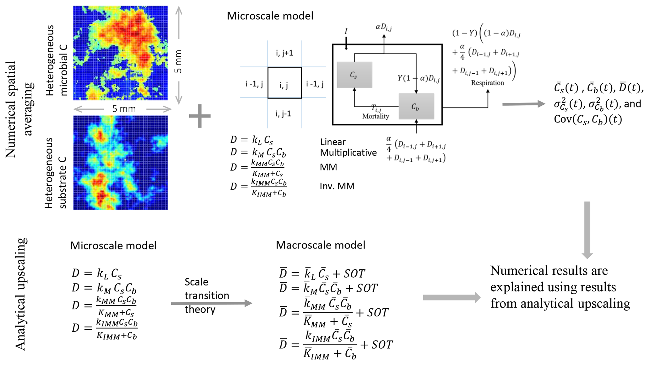
Figure 1Schematic of the two upscaling approaches used to study the C dynamics at the macroscale. Numerical spatial averaging (top): the microscale model is applied at each grid cell of the heterogeneous domain; the mean C pools (substrate and microbial biomass , where the overbar indicates spatial averaging), their mean fluxes, and second-order spatial moments are estimated by Eqs. (24)–(29) at each time step. This approach is referred to as the “distributed model”. Analytical upscaling (bottom): the microscale decomposition flux is dynamically scaled up using scale transition theory, which provides the mean C fluxes as a function of mean C concentrations (mean field approximation) and second-order spatial moments representing the degree of heterogeneity. The deviations from the mean field approximation are denoted as “second-order terms” (SOTs) in the expressions of the mean decomposition fluxes (, where the overbar represents mean quantities). The numerical results obtained from the distributed model are explained using the mathematical expression derived from analytical upscaling. This upscaling scheme is applied to four types of decomposition kinetics (linear, multiplicative, Michaelis–Menten, and inverse Michaelis–Menten).
2.1 Theory
We distinguish between microscale equations valid at the small scale at which the well-mixed assumption holds from macroscale equations valid at a larger scale of interest, which result from the spatial averaging of the microscopic equations. While our derivations are general, in the presented model setup and results, we interpret macroscale as the scale of a small soil core. The goal of spatial upscaling is to derive the macroscale soil C dynamics by the spatial averaging of the microscale dynamics.
To obtain the macroscale dynamics we employ two approaches: (i) a numerical approach based on grid-scale simulations followed by spatial averaging (upper panel, Fig. 1) and (ii) an analytical approach based on scale transition theory (lower panel, Fig. 1). The first is a computationally demanding approach and requires solving the microscale equations at each cell of the domain grid. Spatial averages and variances are thus calculated numerically over the domain at each time point in the simulation. With the analytical approach, the dynamic equations are first averaged and then solved directly for the mean state variables. The obtained analytical expressions are used to interpret the results of the numerical simulations.
To proceed, the spatial average operator for our 2-D domain is defined as
where the double integral extends to the whole 2-D domain, χ is a generic variable (Cs or Cb) or C flux, and Nx and Ny are the number of grid cells in the x and y direction. The second equality allows for the estimation of χ using the simulated time series of the variable of interest in each grid cell (denoted by χi,j). In contrast to numerically solving the problem at each grid cell, the analytical approach derives the dynamics of the macroscale variables and fluxes using scale transition theory, as discussed in Sect. 2.1.2.
2.1.1 Microscale model of soil carbon dynamics
The dynamics of soil organic C in a homogeneous medium are characterized by specific reaction kinetics that define organic C fluxes, as well as the number and arrangement of the soil C pools. For simplicity, we used a two-pool model in which organic C is divided into (i) soil organic carbon substrate (Cs) and (ii) microbial biomass carbon (Cb) (Manzoni and Porporato, 2007; German et al., 2012). This simple structure was selected because it is at the core of most microbial explicit models (Zelenev et al., 2000; Schimel and Weintraub, 2003). It should be noted that conceptually we include in Cs only organic C that is available for depolymerization and not stabilized; in other words, we focus on decomposition timescales of the order of weeks to months. Modeling all the processes (and associated heterogeneity effects) leading to C stabilization is beyond our scope. The typical timescale of diffusive fluxes is given by , where x is the length scale of space discretization and Ddiff is the diffusion coefficient (Hunt and Manzoni, 2015), and the typical timescale of reactive fluxes is given by the turnover time of the substrate; i.e., τreact. The ratio of the two timescales defines the Damköhler number, , which represents the relative importance of mass transport of the substrate via diffusion vs. reaction (Dentz et al., 2011). For a relevant substrate such as glucose, Ddiff is of the order of 10−11 m2 s−1 (Watt et al., 2006), the turnover time is of the order of ∼ 1 d, and the length scale is of the order of ∼ 50 µm. With these values, Da≪1, which characterizes a reaction-limited system in well-mixed conditions. The result of this approximated calculation would not change with reaction timescales of the order of a few hours. Thus, the well-mixed assumption is valid at the scale of a pore of size ∼ 50 µm; we refer to this model as the “microscale model” (Fig. 1).
To include spatial fluxes across grid cells, we implemented a generic mass transfer mechanism. This mechanism is implemented by assuming that a fraction α of the decomposition rate D (i.e., αD) is transferred in equal amounts to the four neighboring grid cells. Hence, in each grid cell microorganisms receive additional C from neighboring grid cells at a rate (). This choice is motivated by the observation that the products of depolymerization are more soluble than stable organic matter and are thus more likely to be transported away from the site of decomposition. Thus, instead of modeling mobile carbon explicitly, we assumed that a fraction of the source of soluble C is transported to neighboring cells. This mass transfer mechanism can be interpreted as a consequence of various types of spatial redistribution, including diffusion or bioturbation. The microscale equations at one grid cell (control volume) take the following form:
where I is the rate of external input of organic C, D is the rate of decomposition, T is the microbial mortality, and Y is the microbial C-use efficiency. The substrate Cs and microbial carbon Cb are the state variables of the microscale model, and their mass balances, Eqs. (2) and (3), describe their temporal evolution. If α=0, no mass transfer occurs and the model reduces to a simplified reactive system with two C pools, whereby grid cells are disconnected and thus independent. If α>0, mass transfer among the grid cells occurs. In this way, by changing the value of α, the effect of spatial redistribution on mean carbon dynamics can be assessed. With α=0, the general mathematical description of the simplified microscale model is given by
where for conciseness we removed the subscripts indicating grid cell positions. The rate of decomposition is described by four commonly used formulations: linear (Eq. 7), multiplicative (M, Eq. 8), Michaelis–Menten (MM, Eq. 9), and inverse Michaelis–Menten (IMM, Eq. 10) (comparisons among these formulations can be found in Schimel and Weintraub, 2003; Wutzler and Reichstein, 2008; Manzoni and Porporato, 2009).
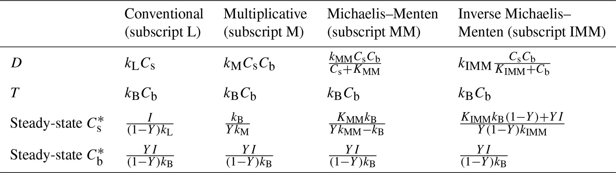
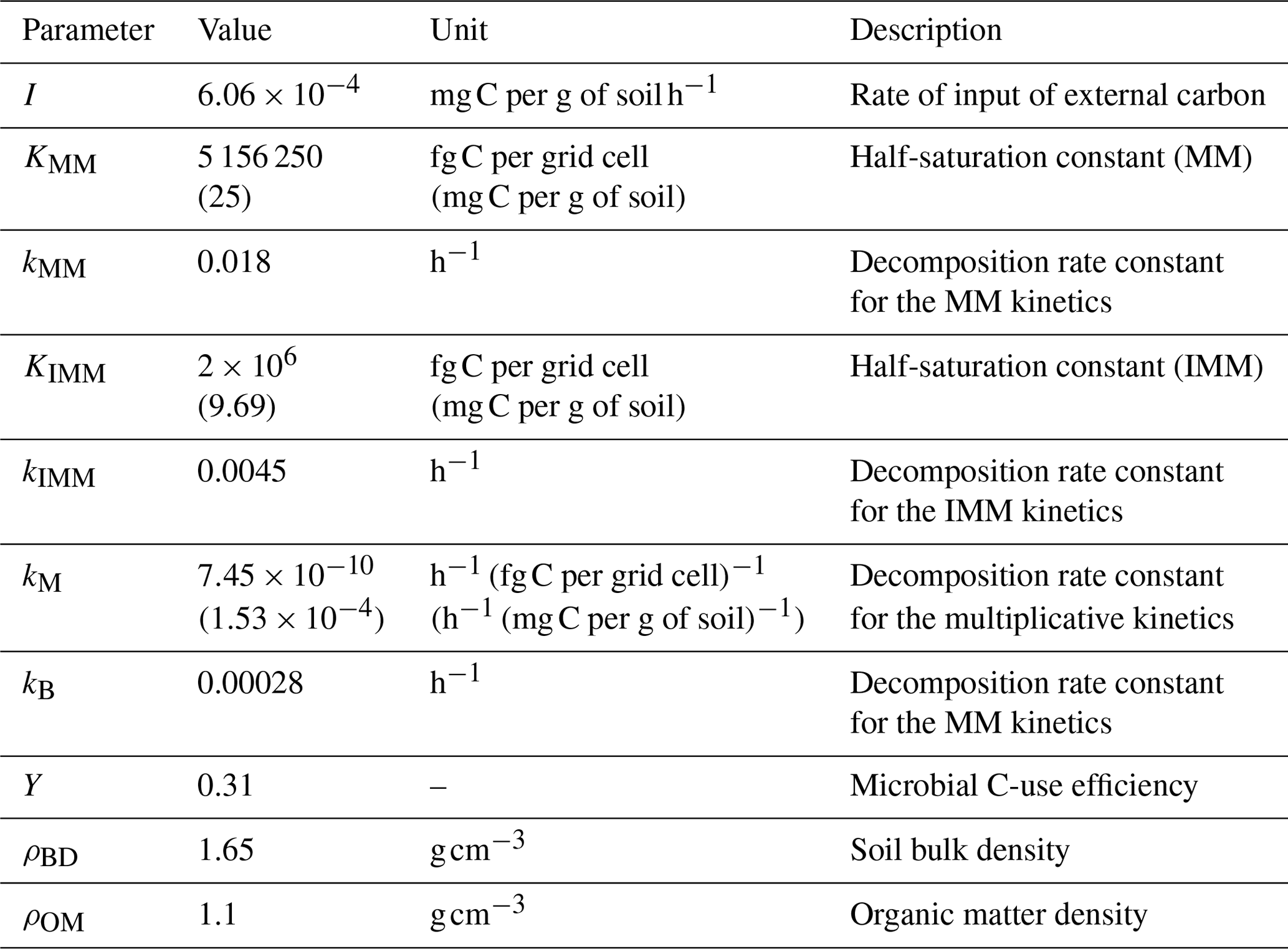
Here, kL, kM, kMM, and kIMM are the decomposition rate constants for linear, multiplicative, MM, and IMM kinetics, respectively; KMM and KIMM are the half-saturation constants for the MM and IMM kinetics, respectively. Table 1 summarizes the functional forms of D and the steady-state solutions to Eqs. (5) and (6) for each case. Microbial mortality is assumed to follow first-order kinetics (T=kBCb). We assume constant temperature and soil moisture conditions so that D is only a function of Cs and Cb. This assumption facilitates an assessment of the role of spatial heterogeneity of C substrates and microbial biomass in our idealized system. The analytical upscaling theory developed in the following section is based on the simplified microscale model given by Eqs. (5) and (6). For the mass transfer model, only the numerical averaging method is used.
Table 1Summary of the microscopic decomposition functions and steady-state solutions.
2.1.2 Spatial upscaling of soil carbon dynamics: scale transition theory
The scale transition theory is applied to study the C dynamics at the microscale and macroscale and to derive the changes in the structure of the equations describing the C pools and their fluxes at the macroscale. To upscale the microscale model, the spatial averaging operator given by Eq. (1) is applied to Eqs. (5) and (6), leading to the governing equations at the macroscale,
where the overbars denote the spatially averaged microscale quantities so that and are the macroscale rates of decomposition and microbial mortality. Since the order of averaging and differentiation can be exchanged, the left-hand side of Eqs. (11) and (12) can be written as and . Moreover, we assume that Y and I are spatially invariant so that averaging does not alter their values. The final mass balance equations for substrate and microbial C at the macroscale are thus given by
where is the mean respiration at the macroscale. In Eqs. (13)–(15), the macroscale variables and can be obtained once the average fluxes and are known. The next step is therefore to express and as a function of macroscale (, ) and microscale state variables (Cs, Cb).
We can generalize the problem and consider a generic microscopic C flux (i.e., D or T) to be a nonlinear (and smooth) function F of state variables Cs–Cb and a parameter vector k , where n is the number of parameters. The spatial averages of Cs, Cb, and k are denoted as , , and . Applying the averaging operator given by Eq. (1) to a multivariate Taylor series expansion of around the spatial average value of Cs, Cb, and and truncating the series to second order gives the macroscopic C flux (a detailed derivation is provided in Appendix A1),
where prime symbols represent variations with respect to the spatial mean values, is the macroscopic C flux, , and are the spatial variances of substrate and microbial C, respectively; is the spatial variance (if i=j) or spatial covariance (if i≠j) between the microscale parameters; , and are the spatial covariances between microscale substrate and microbial C, substrate and parameters, and microbial biomass and parameters, respectively.
In Eq. (16), the first term on the right-hand side, , represents the first-order approximation of , also known as mean field approximation (MFA). The MFAs for the chosen models are for multiplicative kinetics, for Michaelis–Menten kinetics, and for inverse Michaelis–Menten kinetics. Most C cycling models neglect all the other terms in Eq. (16). The remaining six spatial variance and covariance terms in Eq. (16) are collectively referred to as second-order terms (SOTs). Higher-order terms can also be included by truncating the series beyond the SOT. We refer to all terms of order higher than or equal to second order as “high-order terms” (HOTs). When the system is well-mixed, all variances and covariance terms vanish, leaving only the MFA. Therefore, only considering the MFA is equivalent to assuming well-mixed conditions at the macroscale (i.e., Eqs. 5 and 6 are equivalent to Eqs. 13 and 14).
Equation (16) provides a proof that the mean field approximation is a specific case of the more general expression for a macroscopic C flux that also depends on spatial heterogeneity through the SOT. The MFA is valid only when either of the following two conditions are met. First, the microscale decomposition rate is assumed to follow first-order kinetics with homogeneous kL because when F is a linear function of substrate and microbial C, the second-order partial derivatives in Eq. (16) are zero. Second, Cs,Cb, and kinetic parameters are spatially homogeneous because in this case all the second-order moments (spatial variances and covariances) are zero. However, if F is nonlinear, the second-order partial derivatives are nonzero; similarly, if any type of microscale biophysical or biochemical heterogeneity is present, the SOTs in Eq. (16) play a role in determining the macroscopic C dynamics.
Equation (16) illustrates the advantage of using scale transition theory as it provides an approximate analytical relation between the microscale and macroscale quantities, which allows for an immediate assessment of the role of both nonlinearities in the C flux formulations and spatial heterogeneities. Importantly, in some cases, Eq. (16) yields an exact (rather than approximated) equation for macroscale quantities, as shown in the following section.
2.2 Effect of microscale heterogeneities on macroscale dynamics
Depending upon the kinetics of the microscale decomposition model (Table 1), the macroscale is expected to take different forms. Using different kinetic models, we now discuss some specific cases of microscale heterogeneities based on their biophysical or biochemical nature. Biophysical heterogeneity is characterized by the spatially heterogeneous distribution of substrate and microbial C, whereas biochemical heterogeneity is characterized by the spatially heterogeneous distribution of substrate quality and microbial properties, captured by the kinetic parameters. The inaccessibility of SOM can result in C persistence. Therefore, inaccessibility can be modeled (at least at a conceptual level) through low values of the kinetic rate constants, similar to biochemical properties. In the simple model used here, accessibility to substrates or chemical recalcitrance is not mechanistically distinguished, so variations in substrate “quality” in the broadest sense can be interpreted as spatial heterogeneity in either chemical characteristics or accessibility at the microscale.
First, we focus on systems with only biophysical heterogeneity of substrate and microbial C. For the first-order kinetics model, the rate of decomposition is given by D=kLCs, and using Eq. (16) and substituting , we obtain
In Eq. (17), has the same form as D, indicating that microbial implicit first-order kinetic models do not show any sensitivity to spatial heterogeneities because of the linearity of the decomposition function. For the multiplicative model, the rate of decomposition at the microscale is given by Eq. (8), and inserting Eq. (8) into Eq. (16) gives
In Eq. (18), the biophysical heterogeneities play a role through the covariance term . Note that Eq. (18) is an exact equation because all the spatial moments of order higher than the second order are zero. Thus, only the mean state variables and the spatial covariance are needed to fully characterize the macroscale dynamics in this case. Furthermore, a positive spatial covariance (i.e., colocation of substrates and microorganisms) would increase the mean decomposition rate (), whereas a negative spatial covariance (i.e., spatial separation between substrates and microorganisms) would decrease it.
Similar to the multiplicative decomposition model, also in models based on MM and IMM kinetics, the rate of decomposition at the macroscale depends on the covariance term and additional terms representing the spatial variances of the substrate and microbial C (Table 2). The spatial variance terms are always negative because variances are positive quantities and the partial derivatives multiplying the variances are negative in all decomposition functions that saturate at high substrate or microbial biomass concentration. In contrast, the spatial covariance term is positive or negative based on the sign of . Therefore, when using the MM or IMM kinetics, can be the approximated by the MFA only if the variance and covariance balance each other or are both negligible.
Second, we consider only biochemical heterogeneity. In this case, model parameters k vary spatially, but the initial values of the state variables Cs and Cb are assumed homogeneous. With linear decomposition, substituting D=kLCs into Eq. (16) yields
Equation (19) shows that for a biochemical heterogeneous system, even the simplest linear model requires an additional covariance term to describe the governing equations at the macroscale. This covariance term might change the linear microscopic model into a nonlinear macroscopic model. For the multiplicative model (Eq. 8), Eq. (16) yields
where and are respectively the spatial covariances between the state variables Cs–Cb and the rate constant parameter kM. These two additional spatial covariance terms capture the effects of biochemical heterogeneity caused by the spatial variation in the rate constants of decomposition. Similar terms also appear when using the MM and IMM models.
Lastly, we consider a heterogeneous system with combined biophysical and biochemical heterogeneities, denoted as “fully heterogeneous”. Again, we use the multiplicative model to illustrate the relation between the dynamics at the microscale and macroscale. Now, all the state variables and parameters in D at the microscale are spatially variable. For the multiplicative kinetics, kM, Cs, and Cb are spatially variable so that inserting Eq. (8) into Eq. (16) gives
This generalized case includes all the spatial covariances between parameters and the state variables, thereby capturing biophysical and biochemical heterogeneities simultaneously. Moreover, Eqs. (20) and (21) are second-order approximations, but an exact equation can be obtained by including a third-order term . A similar derivation is described for MM and IMM kinetics in the Appendix; however, an exact expression for the macroscale decomposition rate for these two kinetics cannot be found and we only use the second-order approximation. Table 2 provides a summary of the theoretical results for the discussed heterogeneous cases and for all four types of decomposition kinetics.
The same rationale used to derive Eq. (21) can be applied in systems in which the C input rate I or the microbial C-use efficiency Y are not homogeneous as we assumed. This would cause additional second- and higher-order terms to appear in the macroscale equations, with consequences for the overall C balances.
Similar derivations can be done for the microbial mortality rate (F=T). The Taylor expansion of microbial mortality is simpler because we assume T to follow first-order kinetics, implying that all the second-order terms are equal to zero. Therefore, the mean field approximation is exact and the spatial variance of this parameter has no effect on the macroscale dynamics,
To illustrate how macroscale decomposition kinetics are affected by spatial heterogeneity, we define a macroscale specific growth rate (SGR), which is calculated by dividing the mean respiration rate by mean microbial C in the system.
To summarize, we started with the spatial averaging of the SOM dynamics equations at the microscale and applied scale transition theory to derive relations between the microscale and macroscale C fluxes, which depend on both mean state variables and their spatial statistics (Table 2). Thus, to solve the macroscale Eqs. (13) and (14), we still need information regarding the second-order moments, e.g., and . To close the problem mathematically, these moments can be regarded as extra state variables requiring additional differential equations to describe their dynamics (Keeling et al., 2002; Murrell et al., 2004; Barraquand and Murrell, 2013). Alternatively, the second-order moments can be parameterized as empirical functions of first-order terms , , and (Bergström et al., 2006). Here, our goal is to quantify how heterogeneities alter C fluxes in idealized systems, so we leave the closure problem for a future contribution and instead use the numerically simulated dynamics at the microscale to calculate the spatial moments and SOT.
Table 2Summary of macroscale equations for the decomposition rate ().
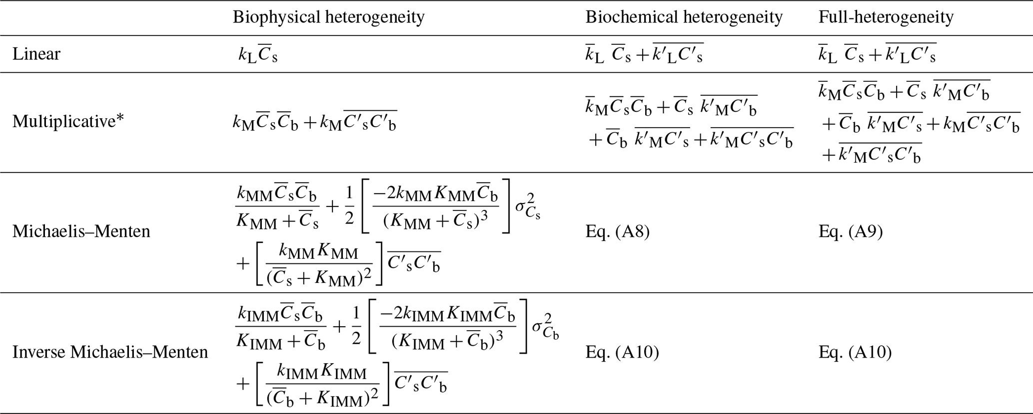
* The expression of for multiplicative kinetics in each heterogeneity case is exact.
2.3 Model setup
As in previous spatially explicit models (Ginovart and Valls, 1996; Allison, 2005; Kaiser et al., 2014), we start with a 2-D domain characterized by an initial heterogeneous field of the substrate and microbial C, and we numerically simulate the dynamics of SOM with the microscale two-pool model in Eqs. (2)–(4) at each cell in the domain. The 2-D domain has 100×100 square grid cells with an edge length of 50 µm, and we populate it with randomly generated initial substrate and microbial C fields. This numerical model is referred to as the distributed model (see Fig. 1). From the solution of the distributed model, the mean behavior of the system (, and ) can be calculated at each time step by using sample statistics of Cs and Cb:
where is specified for multiplicative kinetics; a similar approach was applied for MM and IMM kinetics. Table A1 in the Appendix lists all the parameters related to different kinetic models used in the simulations. We performed the simulations in mass units of femtograms (fg; fg g) and later converted the state variables to concentration units, i.e., milligrams of carbon per gram of soil.
2.4 Initial 2-D random fields of SOM and kinetic parameters
Two-dimensional spatially heterogeneous distributions of substrates and microbial C were generated to run the distributed model. The obtained distributions were based on the following constraints: (i) the total amount of organic C is set, (ii) the total amount of microbial C is 1 % of total organic C, (iii) the maximum amount of C in a cell is set (Eq. A12), and (iv) some grid cells have no microbial biomass. For details on the spatial field generation, see Appendix A2.
To study the effects of the degree of heterogeneity on decomposition, random fields of substrate C with different degrees of correlation with microbial C were generated. We created three cases in which substrate and microbial C were initially positively correlated, negatively correlated, or uncorrelated. The three cases were obtained by applying a linear operator on the microbial C fields with positive and negative slope to obtain positively and negatively correlated substrate C fields, respectively. The uncorrelated substrate C field was generated independently from the microbial C field and can be interpreted as the result of external disturbances disrupting preexisting spatial correlations. The case of positive initial correlation between substrate and microbial C would result in a heterogeneous system with spatial co-occurrence of substrate and microbial C, whereas initial negative correlation would result in isolated patches of substrate and microbial C. In all scenarios, the substrate distributions are normalized to have the same amount of total substrate C, thereby allowing for comparisons among different degrees of heterogeneity (Fig. 2).
To generate a heterogeneous random field for kinetic parameters, we considered a uniform distribution for KMM and KIMM and a log-uniform distribution for kM, kMM, and kIMM (Forney and Rothman, 2012; Manzoni et al., 2012). The log-uniform distributions were defined so that the mean kinetic constants were equal to those of the homogeneous system (Table A1), and their variances were tuned to characterize different degrees of heterogeneity. To generate the initial fields, Nx×Ny random numbers were extracted from the chosen distributions and placed into the 2-D domain. Figure A7 in the Appendix shows the probability densities for two different standard deviations for kMM and kM (the parameters of the distributions are listed in Tables A2 and A3).
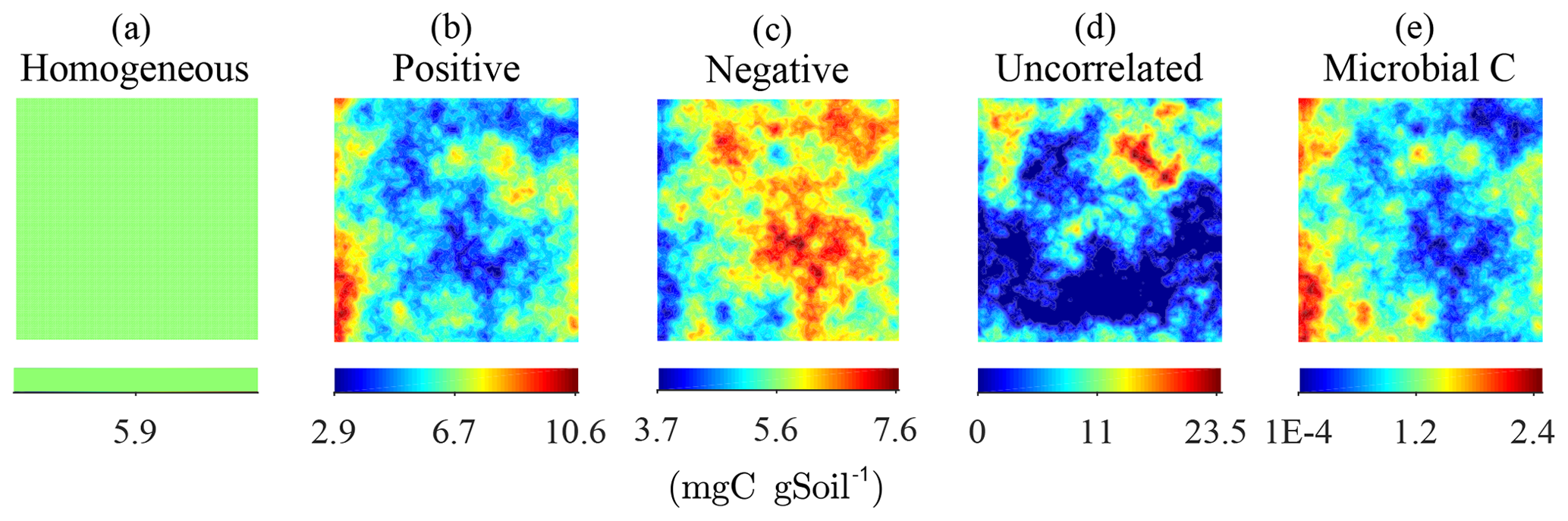
Figure 2Steady-state simulation: examples of the homogeneous (a) and the heterogeneous distributions of substrate C constrained to have the same total amount of substrate C (b–d). The fields in (b–d) were obtained by imposing different degrees of correlation with the initial heterogeneous distributions of microbial C, shown in (e).
2.5 Estimation of kinetic parameters
To choose parameter values for the linear and multiplicative kinetics that allow for comparisons with the MM model, we first simulated the substrate C dynamics at the microscale for a given initial condition and using MM kinetics. Second, we fit the linear and multiplicative kinetics models to the time series obtained using MM kinetics (using the optimization toolbox in MATLAB). In this procedure, we assumed that the microbial mortality constant (kB) was the same for all choices of the decomposition model. The parameters of the inverse MM are chosen (by trial and error) so that the respiration rate in the homogeneous system is comparable to the MM kinetics in the homogeneous system.
2.6 Simulation scenarios
Two scenarios, based on varying initial conditions (ICs), were implemented to investigate the effects of microscale heterogeneities on macroscopic decomposition (Fig. 3).
Scenario 1 (steady-state simulation – SS): in this scenario, the initial heterogeneous field of substrate and microbial C was generated as described in Sect. 2.4. The spatial mean of the initial substrate and microbial C match their steady-state values given by the microscale equations (Eqs. 5 and 6) forced with a constant substrate input. Additionally, a minimum amount of microbial C was set in each cell (values at least 1 order of magnitude lower than those at steady state) to ensure that OM could be decomposed, albeit at a slower rate than elsewhere.
Scenario 2 (high substrate simulation – HS): in this scenario, the initial heterogeneous field of substrate C was perturbed around a value much larger than the steady state as described in Sect. 2.4.
In the HS scenario, simulations were based on three nonlinear decomposition models (multiplicative, MM, and IMM kinetics). However, in the SS scenario, we present results only for multiplicative kinetics because MM kinetics can be approximated by multiplicative kinetics when the substrate is much smaller than the half-saturation constant (KMM), as is the case with the chosen initial heterogeneous substrate field and the values of KMM. Results using the linear decomposition model are not shown because with this model the spatially averaged fluxes are equal to the macroscale flux calculated at the mean C concentration (Eq. 17), as long as kL is homogeneously distributed.
In both scenarios, we explore the effects of biophysical and full heterogeneity on the temporal evolution of the mean state variables (substrate and microbial C) and their associated rates. We used the distributed model to estimate the mean quantities and second-order spatial moments (and thus SOT) for three degrees of biophysical heterogeneity. A homogeneous system in which the initial substrate and microbial C, as well as kinetic parameters, are spatially uniform was always used as a control. The combined effect of biophysical and biochemical heterogeneity was simulated by imposing the spatially heterogeneous kinetic parameters along with the heterogeneous initial substrate and microbial C.
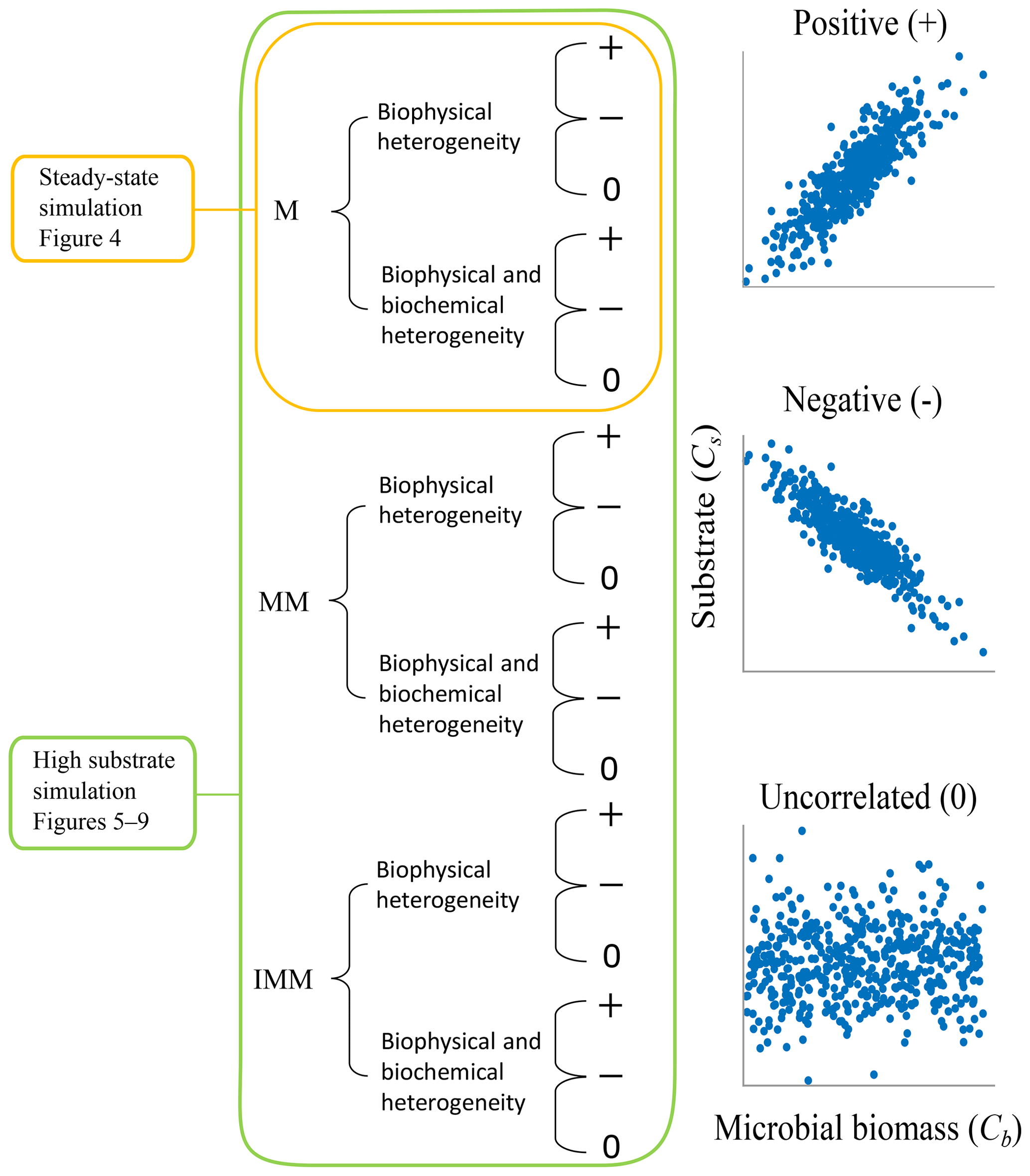
Figure 3Two scenarios were implemented based on the initial spatial distribution of substrate and microbial C. In scenario 1, substrate and microbial C are perturbed around the steady state of the microscale differential equations, and simulations are only carried out with the multiplicative (M) kinetics. In scenario 2, substrate and microbial C are perturbed to values larger than the steady state, and simulations are conducted for multiplicative (M), Michaelis–Menten (MM), and inverse Michaelis–Menten (IMM) kinetics. For each scenario and type of heterogeneity, three different initial distributions of substrate and microbial biomass are considered to be representative of microscale heterogeneities (positively correlated (+), negatively correlated (−), and uncorrelated (0) fields of substrate and microbial C).
3.1 Scenario 1: steady-state simulation (SS)
Figure 4 illustrates the temporal evolution of the macroscopic decomposition dynamics for the three different heterogeneous cases with varying degrees of initial correlation between substrate and microbial C in comparison to the homogeneous system. In Fig. 4, the left and right columns respectively show the effects of biophysical heterogeneity and full heterogeneity on the mean C pools and fluxes (kM is based on the case “biochemical heterogeneity 1” in Table A3). For this analysis, we focus on the multiplicative decomposition model. With the current parameter choice, the ratio of microbial biomass to substrate C attains at steady-state values that are larger than would be expected for ratios of biomass to total soil organic C (Xu et al., 2013). This is due to our interpretation of substrate C as a relatively active fraction of total soil organic C.
Since the mean initial condition corresponds to the steady state of the microscale system, in a homogeneous soil no changes occur in substrate C (solid line in Fig. 4a and b) and microbial C (solid line in Fig. 4c and d), and the mean respiration rate is equal to the constant rate of input of external C (solid line in Fig. 4e and f). In contrast, for the system with biophysical heterogeneity, the mean C pools and respiration () fluctuate towards the steady state of the microscale system as a result of the heterogeneous initial placement of C substrates. Similarly, for the fully heterogeneous system the mean microbial C pool (Fig. 4d) and fluxes (Fig. 4f) fluctuate near their steady-state values, but the mean substrate C pool (Fig. 4b) reaches a new steady state. The value of the new steady state for depends upon the parameters of the log-uniform distribution of kM and is given in Appendix A3.

Figure 4Scenario 1 (steady-state simulation): effect of biophysical (left) and full heterogeneity (right) on the macroscopic decomposition dynamics when the substrate is distributed randomly around the steady state and only considering multiplicative kinetics at the microscale: (a, b) mean substrate C (), (c, d) mean microbial C (), (e, f) mean respiration rate (), and (g, h) sum of second- and third-order terms (∑HOT).
In all heterogeneity scenarios, is initially higher than in the homogeneous system when substrate and microbial C are initially correlated, whereas it is lower when substrate and microbial C are negatively correlated. When substrate and microbial C are uncorrelated, the system exhibits a behavior similar to that of the positively correlated fields but with higher respiration peaks (Fig. 4e). This is caused by the high initial spatial variance of substrate C that resulted in hot spots richer in substrate C than in the positively correlated case (Fig. 2). Furthermore, in the multiplicative kinetics, the respiration flux is proportional to the amount of substrate C so that larger variations in substrate cause larger fluctuations in the mean respiration flux. In the fully heterogeneous system, fluxes show similar dynamics as those in the biophysically heterogeneous system, except for the different steady state. Varying the mean (Fig. A1) and variability (Fig. A2) of kM alters the quantitative, but not qualitative, behavior of the macroscale system (results shown in Appendix A4).

Figure 5Scenario 2 (HS with multiplicative kinetics): effect of biophysical heterogeneity (left) and full heterogeneity (right) on the macroscopic decomposition dynamics when the substrate is distributed around a value higher than the steady state of the homogeneous system: (a, b) mean substrate C (), (c, d) mean microbial C (), (e, f) mean respiration rate (), and (g, h) sum of second- and third-order terms (∑HOT).
Figure 4g and h show the sum of all higher-order terms (∑HOT; see Table 2 for multiplicative kinetics). For a biophysically heterogeneous system, the ∑HOT only includes the spatial covariance term (Eq. 18), but for a fully heterogeneous system it includes the last three terms in Eq. (21) as well as the third-order term . The ∑HOT is initially positive, zero, and negative, respectively, for positively correlated, uncorrelated, and negatively correlated substrate and microbial C, and it exhibits strong temporal variations (Fig. A3). A positive ∑HOT value enhances , whereas a negative value decreases it in all three heterogeneous cases compared to homogeneous . This result is aligned with our expectation from the analytical expression of the macroscale multiplicative model. In systems including both biophysical and full heterogeneity, the sums of the HOTs are stable in the long term, once the steady state has been reached. This was confirmed by running the model for 100 years. Furthermore, any additional perturbation of the new steady state caused by an external factor will reintroduce these fluctuations.
3.2 Scenario 2: high substrate simulation (HS)
3.2.1 Dynamics of substrate and microbial C at the macroscale
Figure 5 illustrates the temporal evolution of the mean properties of the macroscopic decomposition dynamics for multiplicative kinetics for systems with either biophysical (left) or full (right) heterogeneity when the initial condition is perturbed from the steady state by adding C substrates. In this scenario, both homogeneous and heterogeneous systems exhibit transient dynamics because the initial conditions are set far from the steady state. The results in Fig. 5c indicate that, during the microbial growth phase, the production of microbial C is faster when substrate and microbial C are positively correlated or uncorrelated compared to the case of negative correlation. Consequently, at the beginning of the simulation, the mean substrate (Fig. 5a) is decomposed faster due to the higher respiration (Fig. 5e) for the positively correlated and the uncorrelated substrate and microbial C, and it is decomposed slower for the negatively correlated substrate and microbial C when compared to the homogeneous system. By the end of the simulation period, in all heterogeneous scenarios, biomass production and substrate consumption are lower than in the homogeneous system. As in scenario 1, the initial mean respiration for the uncorrelated case is higher than that in the positively correlated case. Moreover, the fully heterogeneous system (Fig. 5, right) shows a similar behavior as the biophysically heterogeneous system, but the peaks of appear earlier for all degrees of correlation between substrate and microbial C.
Similar to Fig. 4, Fig. 5g and h show the sum of all higher-order terms (see Table 2, multiplicative kinetics). For both heterogeneous systems, is higher than the MFA when the ∑HOT is positive, whereas is lower than the MFA when the contribution of these moments is negative. This result agrees with the analytical expression and is valid for all types of biophysical heterogeneities. The ∑HOT for biophysical heterogeneity is initially positive for the positively correlated and uncorrelated substrate and microbial C, but it later becomes negative, whereas it is always negative for the negatively correlated substrate and microbial C. Spatial covariances among kinetic parameters and state variables (i.e., ) also contribute to the ∑HOT in the fully heterogeneous system in addition to . Specifically, the spatial covariance between kM and Cb gives rise to early peaks of (see all HOTs in Fig. A4).
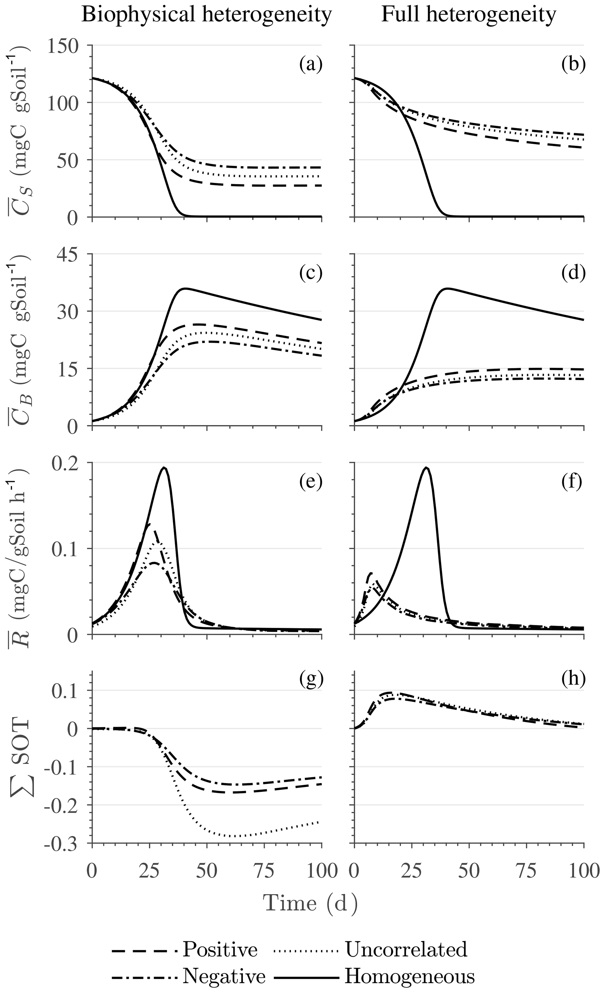
Figure 6Scenario 2 (HS with Michaelis–Menten kinetics): effect of biophysical heterogeneity (left) and full heterogeneity (right) on the macroscopic decomposition dynamics when the substrate is distributed around a value higher than the steady state of the homogeneous system: (a, b) mean substrate C (), (c, d) mean microbial C (), (e, f) mean respiration rate (), and (g, h) sum of second-order terms (∑HOT).
Figures 6 and 7 show similar results as Fig. 5, but for Michaelis–Menten and inverse Michaelis–Menten kinetics, respectively. The transient dynamics of the mean C pools and fluxes differ from those obtained using multiplicative kinetics. For both MM and IMM kinetics, during the initial growth period, the mean respiration rate in the biophysically heterogeneous systems is similar to that occurring in a homogeneous system, but attains lower peaks (Figs. 6e and 7e). As a result, substrate loss (Figs. 6a and 7a) and microbial growth (Figs. 6c and 7c) slow down compared to homogeneous conditions. Interestingly, with MM kinetics, in the uncorrelated case is not higher than in the other heterogeneity cases as occurred with multiplicative kinetics (compare Figs. 6e and 5e). This is because with MM kinetics the respiration flux is limited by the maximum rate of decomposition and not only by substrate availability. In contrast, with IMM kinetics in the uncorrelated case is higher than in the other heterogeneity cases, as it was with multiplicative kinetics. This is because the initial microbial C is often much lower than the half-saturation constant for IMM kinetics, making the IMM decomposition rates numerically similar to those obtained using the multiplicative decomposition model.
The fully heterogeneous system (right panels in Figs. 5, 6, and 7) shows different behavior compared to the biophysically heterogeneous system. The peaks of appear much earlier than in the biophysically heterogeneous system, though the temporal shift of the peak is not as pronounced with IMM kinetics. Additionally, the values of mean fluxes and substrate C pools after the peak are respectively smaller and larger than in the homogeneous system or the system with only biophysical heterogeneity. The smaller mean fluxes are due to the right-skewed probability distribution of the kinetic parameters kM and kMM, which causes slower decay despite the mean values of the kinetic parameters being the same. Mathematically, this behavior is caused by the additional covariances in the fully heterogeneous system as explained in the following paragraph.
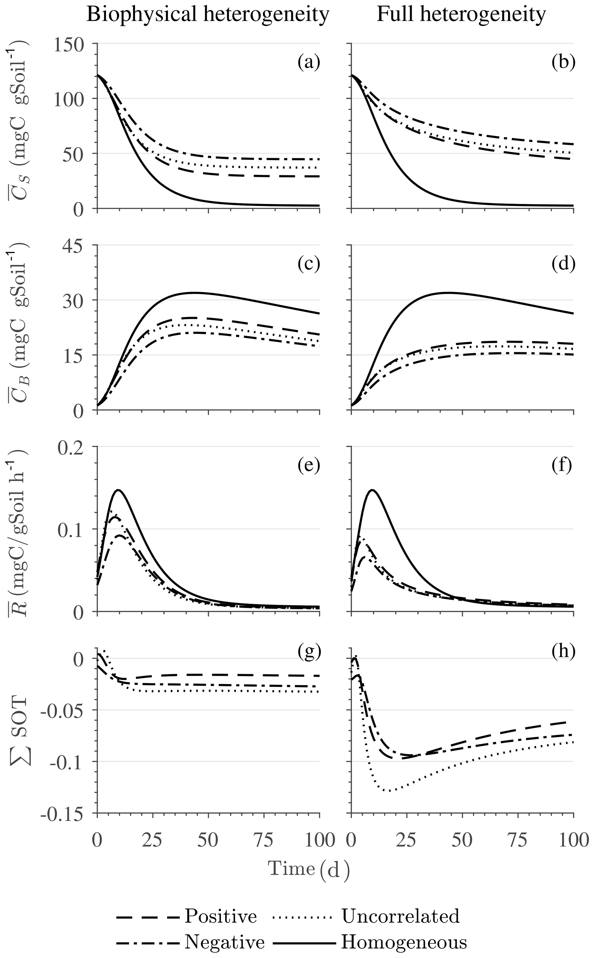
Figure 7Scenario 2 (HS with inverse Michaelis–Menten kinetics): effect of biophysical heterogeneity (left) and full heterogeneity (right) on the macroscopic decomposition dynamics when the substrate is distributed around a value higher than the steady state of the homogeneous system: (a, b) mean substrate C (), (c, d) mean microbial C (), (e, f) mean respiration rate (), and (g, h) sum of second-order terms (∑HOT).
3.2.2 Dynamics of the second-order terms
The ∑SOT (same as ∑HOT but now limiting the HOTs to second order) for MM and IMM kinetics for the biophysically heterogeneous system is given by the sum of the last two terms of in Table 2, and for the fully heterogeneous system it is given by the last eight terms of Eqs. (A9) and (A10), respectively. For the biophysically heterogeneous system, the values of ∑SOT (Figs. 6g and 7g) are initially positive (very small in magnitude) for the positively correlated substrate and microbial C and later become negative, while for the negatively correlated case ∑SOT is always negative. For uncorrelated substrate and microbial C, ∑SOT is initially negative in MM kinetics but mildly positive in IMM kinetics and later becomes negative. Furthermore, the balance between variance and covariance terms makes the MFA a good approximation of only when the combined second-order terms are negligible, which is not the case in this example (see Figs. A5 and A6). The ∑SOT of the fully heterogeneous system for MM kinetics is positive for the first 100 d of simulation and then negative onward, even though the heterogeneous is smaller than the homogeneous (Fig. 6h). This initial positive ∑SOT is driven by the sixth SOT in Eq. (A9), i.e., because grid cells with a high amount of microbial C and a high rate constant cause the covariance to be positive. This covariance becomes negative only after microbial C nears the steady state.
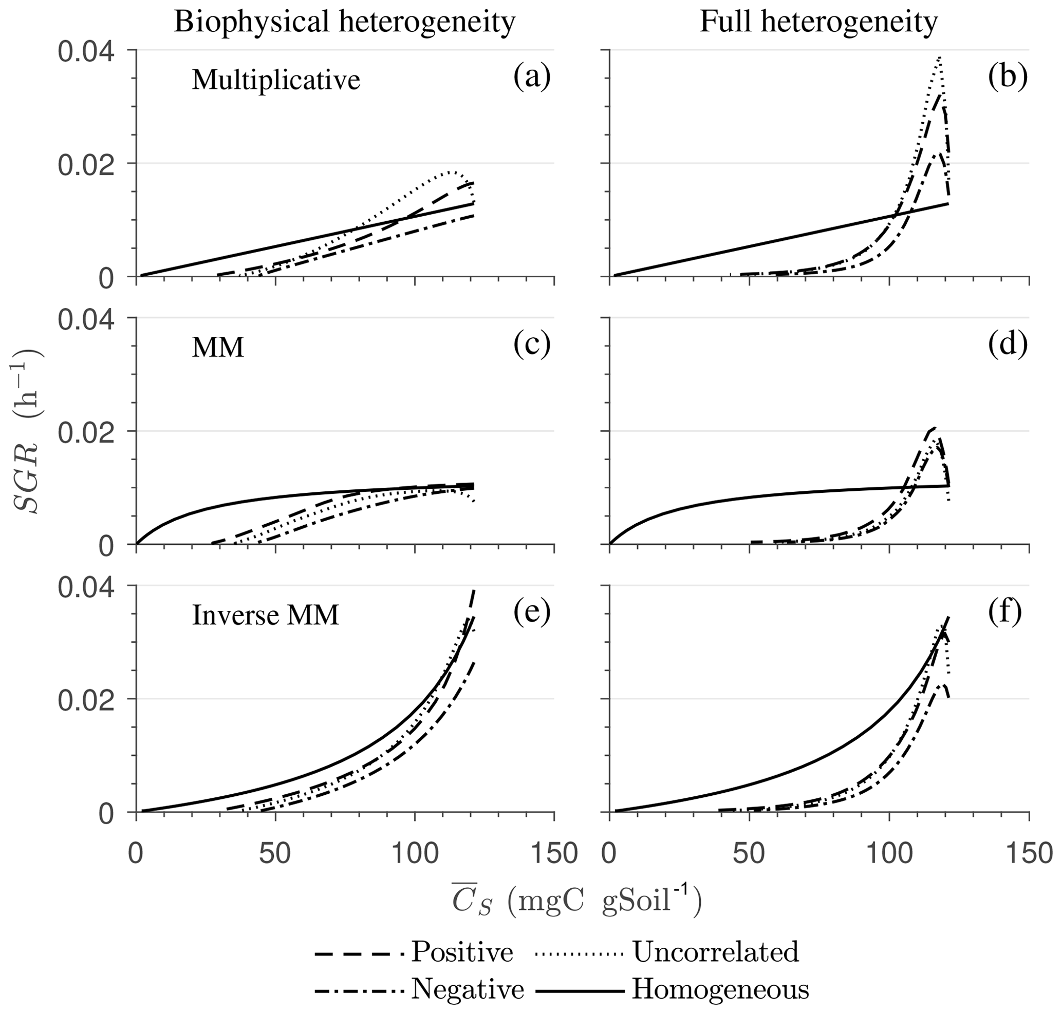
Figure 8Effect of spatial heterogeneity on the mean specific growth rate (SGR) for the HS scenario with the simplified microscale model (no C redistribution): the effect of biophysical (a, c, e) and full (b, d, f) heterogeneity on the mean SGR as a function of mean substrate C () for (a, b) multiplicative, (c, d) Michaelis–Menten, and (e, f) inverse Michaelis–Menten kinetics. Time progresses from right to left as is depleted.
3.2.3 Emerging macroscopic kinetics
Figure 8 highlights the effects of spatial heterogeneities on the mean specific growth rate (SGR) for multiplicative (panels a, b), MM (panels c, d), and IMM kinetics (panels e, f). The depicted SGR curves can be interpreted as the macroscopic kinetic laws emerging from the spatial averaging. For all three kinetics, the functional relation between the mean SGR and for the heterogeneous system depends upon the initial degree of heterogeneity. In contrast, in the homogeneous system the mean SGR is a linear, saturating, and nonlinearly increasing function of Cs for the multiplicative, MM, and IMM kinetics, respectively. The effects of biophysical heterogeneity in all kinetic models are shown in Fig. 8a, c, and e. The negative correlation between substrate and microbial C leads to lower SGR than in the homogeneous system, even if both heterogeneous and homogeneous systems have exactly the same amount of total initial substrate and microbial C. In the case of positive correlation, the initial mean SGR is higher than in the homogeneous system, but in the later phase of decomposition, mean SGR becomes lower. Thus, when the substrate is colocated with the microorganisms, the mean SGR is initially higher but it decreases at a faster rate as the substrate is decomposed when compared to the homogeneous system. If substrate and microbial C are uncorrelated, the SGR functional response remains between the negative and the positive correlation cases.
In the fully heterogeneous system (Fig. 8b, d, and f), the nonlinear character of the relation between mean SGR and increases compared to the biophysically heterogeneous system. Interestingly, the mean SGR in the case of negative correlation for multiplicative and MM kinetic models is higher (for high ) than for the homogeneous system, despite the colocation of substrates and microorganisms being less likely. This behavior is caused by the occurrence of patches with a high turnover rate that control the mean SGR (Fig. 8b and d). In contrast, for IMM kinetics, the mean SGR in the case of negative and positive correlation is lower than the homogeneous system. This behavior might be a consequence of the chosen value of KIMM; i.e., in our parameterization of the IMM kinetics, initially the system is limited by microbial C, resulting in a relatively low decomposition rate and dynamics comparable to those obtained with a multiplicative model (see Fig. 8e, f).
In Fig. 9, we show the specific growth rate as a function of substrate C and α for an uncorrelated initial distribution of substrate and microbial C, as well as for all three kinetics – multiplicative, Michaelis–Menten, and inverse Michaelis–Menten. When α=0, the results in Fig. 9 are the same as in Fig. 8 for the uncorrelated case. When α>0, microorganisms that were initially deprived of substrate now receive additional substrate from neighboring grid cells. As a consequence of this improved substrate availability, microorganisms can consume all the substrate in the long term, whereas without mass transfer some C remains undecomposed (Figs. 5b, 6b, and 7b).
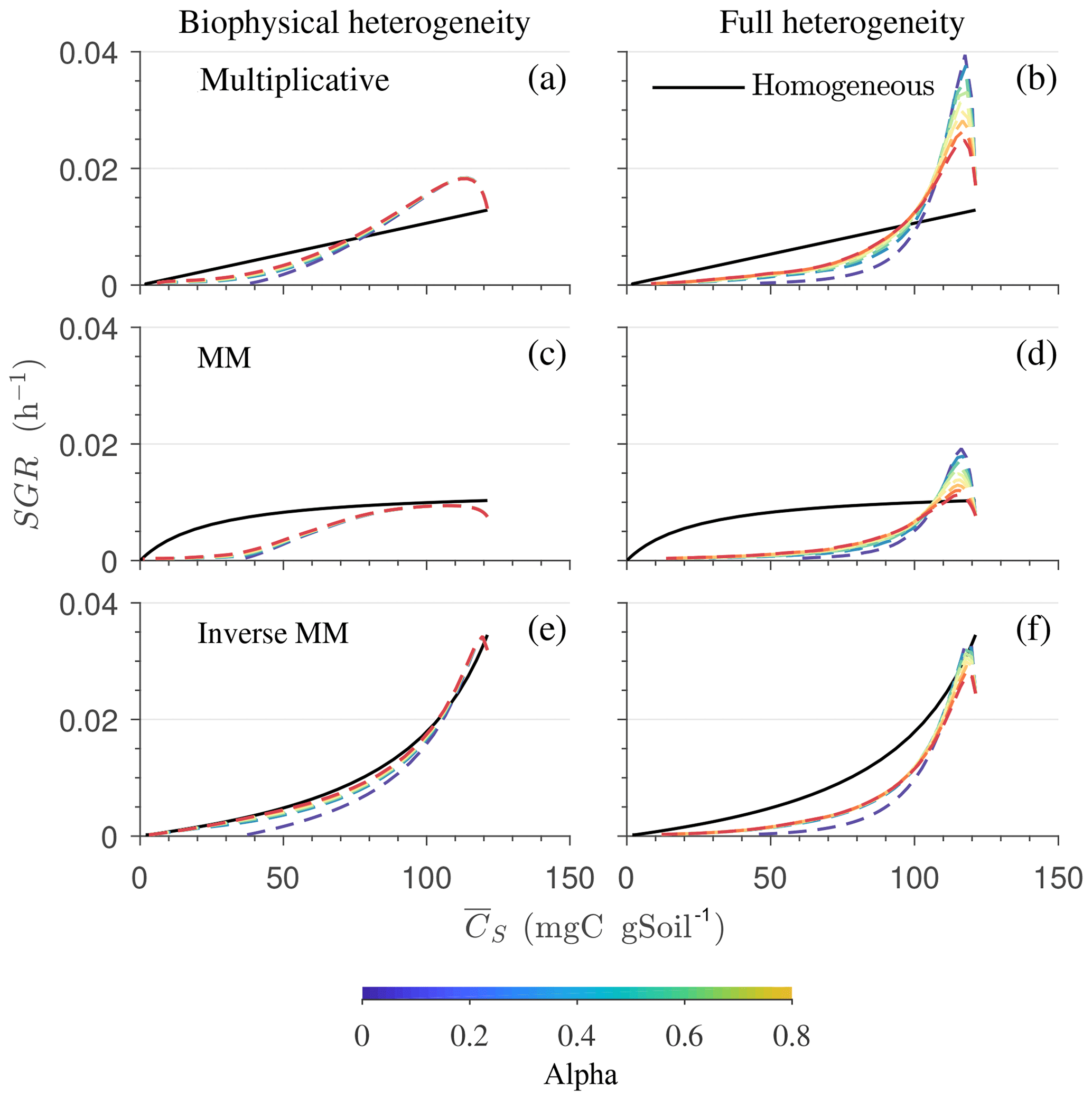
Figure 9Effect of spatial heterogeneity on the mean specific growth rate (SGR) for the HS scenario including C redistribution: effect of biophysical (a, c, e) and full (b, d, f) heterogeneity on the mean SGR as a function of mean substrate C () for an uncorrelated initial distribution of substrates and microorganisms. The three horizontal panels are for (a, b) multiplicative, (c, d) Michaelis–Menten, and (e, f) inverse Michaelis–Menten kinetics. Different colors represent varying values of α. Time progresses from right to left as is depleted.
4.1 Predicted effects of spatial heterogeneity on decomposition
The heterogeneous spatial distribution of organic matter in soils is a result of complex physical, chemical, and biological processes. Both the experimental quantification of the effects of heterogeneity on SOM dynamics (Kravchenko and Guber, 2017) and capturing such effects in mathematical models (Wieder et al., 2015) are challenging. Here, we used scale transition theory, applied to a two-pool model, as a simple approach to analytically account for spatial heterogeneities and scale up SOM dynamics in idealized scenarios that cover different types of spatial heterogeneity. Even with the simplest scenarios, the macroscopic decomposition dynamics of a heterogeneous system differ from those predicted from the mean field approximation (equivalent to assuming well-mixed conditions). This difference in the dynamics at two spatial scales arises because the spatial averaging of the nonlinear kinetics at the microscale creates additional terms in the macroscale equations that depend on the spatial distribution of organic matter and microorganisms (i.e., the second-order spatial moments – SOTs).
These second-order terms represent corrections to the mean field approximation and depend on the spatial variability and covariation of the state variables (i.e., Cs, and Cb). Our numerical results showed that the second-order spatial moments have their own dynamics that drive the heterogeneous system away from the mean field approximation. Notably, while it is recognized that spatial distributions at the microscale affect macroscale dynamics (Falconer et al., 2015), none of the current spatially lumped SOM models include second- or higher-order terms that depend on microscale heterogeneity (see Sect. 4.3).
The simplicity of the microscale model and the derived analytical expressions is such that specific insights on how heterogeneity shapes microscale decomposition patterns can be gleaned and hypotheses generated. The main predictions of this model are the following.
-
Perturbing a system that is initially homogeneous and at steady state by redistributing substrates triggers fluctuations around the steady state (Fig. 4).
-
When only biophysical heterogeneity occurs, in the early microbial growth phase, macroscopic C fluxes are enhanced by the colocation of substrates and microorganisms and reduced when they are isolated (Fig. 8a, c, e).
-
Combined biophysical and biochemical heterogeneity enhances C fluxes in the early stage of decomposition but reduces them in the later stages compared to a homogeneous system (Fig. 8b, d).
-
Both biophysically and fully heterogeneous systems result in a transient persistence of SOM (Figs. 5a, b, 6a, b, and 7a, b). In the biophysically heterogeneous system at steady state, all C is eventually decomposed, whereas in the fully heterogeneous system more C is retained as the substrate pool reaches a new equilibrium (Appendix A3).
-
For a successive reduction in the degree of heterogeneity (i.e., systematically moving from a heterogeneous to a homogeneous system), macroscale dynamics converge to the mean field approximation; i.e., the same kinetics can be used at all scales (Sect. 2.1.2).
-
Increasing local connectivity among grid cells moderately reduces the effect of spatial heterogeneity on the macroscale variables and fluxes.
-
The inverse Michaelis–Menten kinetics appear to be less sensitive to the scale transition than multiplicative and Michaelis–Menten kinetics, but this result might depend on the specific choice of parameter values (for a discussion on scale invariance of upscaled kinetics for reaction networks, see Tang and Riley, 2017).
Our analysis suggests that the persistence of SOM in heterogeneous systems may be a consequence of the microscale heterogeneity in soil carbon cycling. In the transient simulations with biophysical heterogeneity, persistence is a result of spatial disconnection between substrates and microorganisms, captured in our framework by a low probability of colocation at the beginning of the simulation. In the transient simulations for the fully heterogeneous systems, persistence is a result of the combined effects of a low probability of colocation and a high probability of a low decomposition rate constant at the beginning of the simulation. The heterogeneity in substrate quality thus explains the higher persistence of SOM in the fully heterogeneous system compared to the biophysically heterogeneous system.
4.2 Linking theory and observations
We studied three initial heterogeneous distributions of substrate and microbial C: positive, negative, or no correlation between these two variables. These heterogeneities may correspond to spatial aggregation, isolation, or the random occurrence of substrate and microorganisms, respectively. Spatial aggregation is expected in litter and in the surface soil where substrate is abundant and microbial colonies are formed around hot spots (Nunan et al., 2003). Spatial isolation is more likely to occur in the subsoil because of lower substrate and microorganism density as well as poor pore connectivity (Ekschmitt et al., 2008; Salomé et al., 2010), and C-rich patches occur around roots that are separated by large (in a relative sense) volumes of soil that only receive diluted resources via percolation, diffusion, and bioturbation (Kuzyakov and Blagodatskaya, 2015). Uncorrelated spatial fields of substrate and microorganisms may correspond to spatial distributions between these two extremes. There are other examples of contrasting homogeneous vs. heterogeneous conditions. Disturbed, sieved, or dispersed samples may be considered homogeneous, whereas intact soil samples retain their natural heterogeneity.
Despite the correspondence of our idealized heterogeneity scenarios with conditions in natural soils or soil samples, linking our model predictions to observations is challenging, mostly because the effects of heterogeneity cannot be easily isolated in experiments or field observations. Experiments studying the effects of soil structure on the dynamics of SOM mineralization (Killham et al., 1993; Stenger et al., 2002; Ruamps et al., 2011; Juarez et al., 2013; Negassa et al., 2015; Herbst et al., 2016) may introduce other types of heterogeneities that are not dealt with here. For example, samples with different pore networks (Ruamps et al., 2011) likely exhibit different water and air diffusive pathways, which in turn affect microbial respiration (Manzoni and Katul, 2014; Herbst et al., 2016; Koestel and Schlüter, 2019). When targeting experiments to test our upscaled equations, using data from previous studies is challenging because (i) spatial distributions of substrate and/or microbial C are not changed in a controlled manner and (ii) the scale at which physical treatments are performed is probably larger than the scale at which heterogeneity affects C dynamics.
Thus, experiments in which soil structure was manipulated do not allow for the direct testing of the predicted links between heterogeneity and decomposition kinetics at the macroscale. Further, an experimental validation of the present work should stem from designing microscale experiments using artificial porous media with different degrees of heterogeneity. Recent applications of micro-fluidics in soil science (Stanley et al., 2016; Aleklett et al., 2018) could allow for the isolation of the effect of spatial heterogeneity. If any difference is observed among heterogeneous systems, then our framework could be used to attribute these differences to spatial heterogeneity at the microscale. While the proposed mathematical framework is conceptually useful, it is thus challenging to test. Nevertheless, the prediction that the colocation of microorganisms and substrates promotes decomposition is consistent with and theoretically explains the results of recent experiments (Don et al., 2013; Schnecker et al., 2019).
4.3 Developing soil carbon cycling models that account for microscale heterogeneity
Historically, linear microbial implicit models were developed to explain long-term loss of C from agricultural soils or regional-scale variations in SOM (Jenny et al., 1949; Olson, 1963; Jenkinson and Rayner, 1977; Parton et al., 1987). However, when applied at fine spatial or temporal scales, these models fail to describe the dynamics of SOM (Zelenev et al., 2000; Manzoni and Porporato, 2007). To fill this gap and describe microbial processes at the macroscale, nonlinear microbial explicit models have been proposed (Schimel and Weintraub, 2003; Manzoni and Porporato, 2009; Xie, 2013). In contrast to these approaches that impose nonlinear kinetics at the macroscale, here we started from the assumption that SOM kinetics are either linear or nonlinear at the microscale and let scale transition theory determine the type of kinetics at the macroscale.
Conceptually, this approach is similar to upscaling chemical reaction networks to obtain a compact kinetic law that only depends on the concentrations of reactants and products (Tang and Riley, 2013, 2017). However, here we focus on spatial heterogeneity rather than on the complexity of chemical reactions. In a more complete upscaling approach, both sources of microscale variability should be taken into account.
When assuming linear kinetics at the microscale, we showed analytically that the kinetics at the macroscale remain linear and independent of soil biophysical heterogeneity (Eqs. 17 and 22). This result has implications for experimental studies linking soil architecture to SOM mineralization. In some of these studies, first-order microbial implicit kinetics are used to describe the data (Bouckaert et al., 2013; Juarez et al., 2013). If a linear model captures the SOM dynamics in a heterogeneous system well, then either the underlying microscale dynamics are indeed linear, or the averaging of underlying nonlinear equations leads to linearity at the macroscale.
Conversely, we demonstrate that nonlinear kinetics at the microscale do not remain the same when scaling up. The macroscale dynamics retain a clear signature of nonlinearities at the microscale in the MFA term, but the second-order terms could be even more important than the MFA. Thus, nonlinear kinetics might improve SOM predictions because microbial activity is accounted for (Wieder et al., 2013) (at the cost of increased uncertainty; Wieder et al., 2018), but the question remains: which kinetic formulation should be used at the macroscale to capture both microbial activity and spatial heterogeneities? We offer a framework to advance this area by using appropriately upscaled nonlinear kinetics including SOT at the macroscale. This upscaling framework can be extended to account for the role of other microscale interactions, such as among substrates, microorganisms, and minerals, or even temporally varying connectivity due to water movement. These improvements, however, would come at the cost of an increased number of nonlinear second-order spatial moments.
To summarize, the proposed theoretical developments allow for the integration of spatial heterogeneity into decomposition kinetics. Assuming that the second-order spatial moments are known, this integration can be achieved by using the equations listed in Table 2 instead of standard linear or nonlinear kinetic equations used in current models (Wieder et al., 2018; Abramoff et al., 2018). However, the second-order moments and their dynamics are not known in general, as discussed at the end of the following section.
4.4 Limitations of the upscaling approach
To illustrate the effects of spatial heterogeneities alone, we simulated idealized laboratory conditions in which the environmental conditions are constant so that the decomposition rate is not affected by soil moisture and temperature changes through time and space. Moreover, the simulated domain is small compared to an actual soil sample, but we regard the number of simulated grid cells (104) as representative of the range of variation occurring in larger, similarly idealized samples. In other studies, more complex microscale models based on nonlinear reactive and diffusive fluxes have been implemented (Monga et al., 2008, 2014; Nguyen-Ngoc et al., 2013); however, their spatial upscaling would require the volume averaging of the coupled transport and reaction equations, making the problem mathematically intractable when aiming for analytical solutions (Whitaker, 1999; Valdés-Parada et al., 2009; Porter et al., 2011; Lugo-Méndez et al., 2015). The two-pool microscale model with initial heterogeneous distributions of substrate and microorganisms as described in this study offers a simplified way of simulating reaction–diffusion systems. The two end-member cases of homogeneous and fully heterogeneous systems in which grid cells are independent are representative of conditions in which diffusivities are high compared to reaction kinetics in the former and negligible in the latter. In more realistic settings, conditions are likely to be intermediate between these two cases, as described by varying the value of the mass transfer coefficient α (Fig. 9).
Including C redistribution as a simple mass transfer process does not allow for the study of how soil structure affects macroscale dynamics by creating and maintaining heterogeneous distributions of resources and oxygen, such as in aggregates (Keiluweit et al., 2017; Ebrahimi and Or, 2018). These patterns result from the interaction of transport and reaction processes that the proposed idealized models cannot capture.
The upscaling mechanism described in this work assumes that microbial mortality is first order in microbial C so that this term remains structurally similar in the macroscopic Eqs. (13) and (14). A nonlinear mortality generalized by (Georgiou et al., 2017) would create an additional term in the macroscale equations. The mean microbial mortality can be calculated by inserting the nonlinear T into Eq. (16), resulting in , where is the spatial variance of microbial C (for the biophysically heterogeneous system; i.e., kB is spatially invariant). For β=1, the first-order mortality is recovered (Eq. 22); for has an additional positive variance term that increases mortality at the macroscale.
Finally, the upscaled macroscale equations still require a closure scheme for integration, i.e., a set of equations linking the spatial moments to the mean state variables. With such a set of additional equations, the problem becomes mathematically “closed”, as the only remaining unknowns are the mean state variables. Examples of closure from other fields are mentioned in the Introduction (e.g., Bergström et al., 2006), but finding a robust closure scheme remains challenging and will be the subject of future work.
Moreover, our derivations are general, but how these closure equations are formulated and parameterized will likely depend on the scale transition under consideration – soil pore to core (as in this work), soil core to field, or even field to landscape. It is possible that a whole hierarchy of scale transitions is required to determine the macroscale equations suitable for regional- or global-scale applications. Along similar lines, the number of terms in the Taylor expansion that should be retained at each level of this hierarchy remains an open question. It is also possible that the dynamics at the microscale, in combination with C redistribution, lead to low values of higher-order moments because substrate consumption, the mortality of the microorganisms, microbial mortality, and transport contribute to smoothing spatial gradients.
Most carbon cycling models implicitly assume a spatially homogeneous distribution of SOM in different C pools and are based on the mean field approximation of the rate of decomposition. However, the assumption of homogeneity is adequate only at the microscale in soils due to the homogenizing effect of diffusion, which brings carbon sources and decomposers into direct contact with each other at such scales. Therefore, the mean field approximation is valid only at the microscale, creating a challenge when developing SOM models at the macroscale that also account for environmental heterogeneity. In this contribution, we used scale transition theory to establish an analytical expression for the macroscopic mean decomposition rate that accounts for the microscale heterogeneities. Unlike the mean field approximation adopted in most C cycling models, the upscaled governing equations we derived include second-order spatial moments, i.e., spatial variances and/or covariances between microscale state variables and model parameters. The dynamical behavior of the second-order terms drives the heterogeneous system away from the mean field approximation. For a heterogeneous system initially near steady state, microscale heterogeneities led to oscillations in the macroscale respiration flux and higher SOM persistence in a fully heterogeneous system. For a heterogeneous system perturbed from its equilibrium, the colocation of substrate and microorganisms increased macroscopic C fluxes compared to a case in which they were isolated.
In conclusion, this work provides a methodology to explicitly include microscale heterogeneity in soil C cycling models. Our upscaled kinetic equations could be used in lieu of current formulations, but additional equations describing the dynamics of spatial moments should be further developed to mathematically close the problem. The upscaled equations show that (i) heterogeneities alter the form of the carbon flux equations at the macroscale, and as a result (ii) the colocation (isolation) of microorganisms and their substrates promotes (suppresses) carbon fluxes in soils.
A1 Derivation of the macroscale rate of decomposition
Here we describe the derivation of the spatially averaged C flux for a generic microscopic C flux using scale transition theory. As a first step, we calculate the multivariate Taylor's series expansion of around the spatial average value of Cs, Cb, and k,
where represents the higher-order terms and the overbars denote the spatially averaged microscale quantities.
Second, the averaging operator given by Eq. (1) is applied in Eq. (A1). Truncating terms above the second-order terms, Eq. (A1) becomes
In Eq. (A2), the first-order partial derivatives (second, third, and fourth term between the square brackets) disappear, because the partial derivatives evaluated at the mean state variables are constants that are multiplied by the expectation of the deviation of a quantity, which is zero , where χ is CS,Cb, or k).
Finally, after applying the averaging operator, deviations multiplying the second-order partial derivatives become spatial variances and covariances. As a result, the macroscale C flux is obtained:
Equation (A3) can be used to obtain the macroscale C flux given the decomposition function D at the microscale. Explicit solutions for the multiplicative kinetics are reported in the main text (Eqs. 18, 20, and 21).
For illustration, here we report the derivation of the spatially averaged rate of decomposition for Michaelis–Menten (MM) kinetics. The microscale rate of decomposition for MM kinetics is given by
where both the parameters kMM and KMM and the state variables Cs and Cb are considered spatially variable quantities. Inserting Eq. (A4) into Eq. (A3) gives the macroscale rate of decomposition:
The partial derivative of F with respect to kMM and Cb is zero because F is a linear function of kMM and Cb. Now, for a biophysical heterogeneous and biochemical homogeneous system, covariances and variances related to parameters are zeros so that we are left with
Calculating the derivatives gives
For a biophysical homogeneous and biochemical heterogeneous system, covariances and variances of state variables (Cs and Cb) are zeros so that we are left with
For a completely heterogeneous system with biophysical and biochemical heterogeneity, the mean rate of decomposition at the macroscale is given by Eq. (A9):
Similar to MM kinetics, the mean rate of decomposition for a completely heterogeneous system for IMM kinetics can also be calculated as
A2 Initial 2-D random fields of substrate C and microbial C
The heterogeneous field of microbial C was created using a random field generator that provides 100×100 spatially correlated random numbers between −1 and 1 (Lennon, 2000). These values were then rescaled by an appropriate mean and standard deviation of microbial C. To simulate the dead zones in the heterogeneous system, some grid cells were forced to have no microbial C (the obtained field is denoted yi,j). Moreover, to allow for comparison among simulations, the microbial C field was renormalized to have a specified value of total initial microbial C:
It is assumed that Cb,total is equal to 1 % of the total amount of substrate in the domain (Witter, 1996), which is in turn calculated as , where is the initial mean substrate C in a single grid cell (fg). The amount of substrate C in any grid cell is limited by the maximum amount of C that the cell can accommodate, according to the density of organic matter (ρSOM) and assuming that 50 % of organic matter on a mass basis is composed of organic C. The maximum amount of substrate C that one cell can contain is thus given by
where cellvolume is the volume of a grid cell. The value of was chosen so that the maximum C amount at a micro-site does not exceed Cmax. To summarize, the obtained spatially heterogeneous random fields of microbial C and substrate C satisfy the following constraints: (i) the total amount of organic C is set, (ii) the total amount of microbial C is 1 % of total organic C, (iii) the maximum amount of C in a cell is set (Eq. A12), and (iv) some grid cells have no microbial biomass.
Table A1List of parameters. Values in brackets correspond to the units reported in brackets.
A3 Steady-state substrate C for multiplicative kinetics in fully heterogeneous systems
The substrate C at steady state for all decomposition kinetics is given in Table 1 and is restated here for multiplicative kinetics only:
where * represents steady-state conditions. Equation (A13) shows that the steady-state substrate C depends only on the kinetic parameters and microbial C-use efficiency. Thus, if the kinetic parameters are spatially variable (i.e., a fully heterogeneous system) then is also spatially variable and different from the steady-state values of biophysically heterogeneous or homogeneous systems. Knowing the probability distributions of the kinetic parameters, the mean steady-state substrate C in the fully heterogeneous system can be calculated as the mean value of .
The mean value of a generic function, g(x), is given by , where fX(x) is the probability density function of x. Accordingly, the mean value of is given by
where f(kM) is the probability density function of kM. As in Forney and Rothman (2012), we can assume that the kinetic constant kM follows a log-uniform distribution , with mean where a and b are the parameters of log-uniform distribution. With this distribution the mean becomes
Equation (A15) shows that in the heterogeneous system deviates from the value attained in a homogeneous system because in general kM differs from . Similar derivations can be made for the other formulations of decomposition kinetics.
A4 Sensitivity of simulated fluctuations to changes in kM in scenario 1
We performed two sensitivity analyses in which we altered the kinetic constant parameter for the multiplicative decomposition model kM: (1) decreasing kM in the system with biophysical heterogeneity–positively correlated Cs and Cb (Fig. A1) and (2) increasing the heterogeneity of kM (by increasing its standard deviation) in the full heterogeneity case (Fig. A2). From Fig. A1, it is clear that decreasing the rate constant increases the amplitude and wavelength of the oscillations. As shown in Fig. A2, increasing the heterogeneity of the rate constant increases the amount of undecomposed substrate C compared to a lower degree of heterogeneity (Fig. 4). This pattern can be explained using the analytical expression of the steady-state substrate C (see Eq. A15 in Appendix A3). For the increased heterogeneity case shown in Fig. 4, we used values of a and b as listed in Table A3 for biochemical heterogeneity 1 and multiplicative kinetics, wherein a and b have the same meaning as in Eq. (A15). The analytical expression for the steady state, evaluated with these values of a and b, results in exactly the same steady state of substrate C as simulated by the distributed model (i.e., 15 mg C per g of soil).
These fluctuations are similar to those noted in earlier papers using spatially lumped models (Manzoni and Porporato, 2007; Sierra and Muller, 2015). These papers showed that the occurrence and amplitude of the fluctuations depend on the kinetic parameter values, as is the case here.
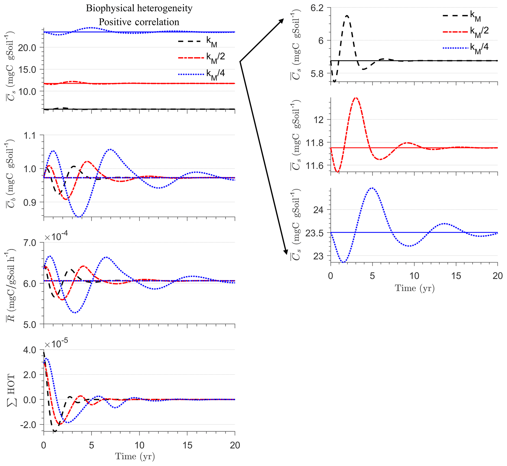
Figure A1(a) Mean substrate C (), (b) mean microbial C (), (c) mean respiration rate (), and (d) sum of second- and third-order terms (∑HOT) are shown as a function of time for positively correlated initial spatial heterogeneity of Cs and Cb. This figure is similar to Fig. 4 (initial substrate is distributed randomly around the steady state). Varying levels of the rate constant kM are shown (as indicated by different line styles and colors; the base case is the same as in Fig. 4). Panels on the right are enlarged views of the time trajectories of .
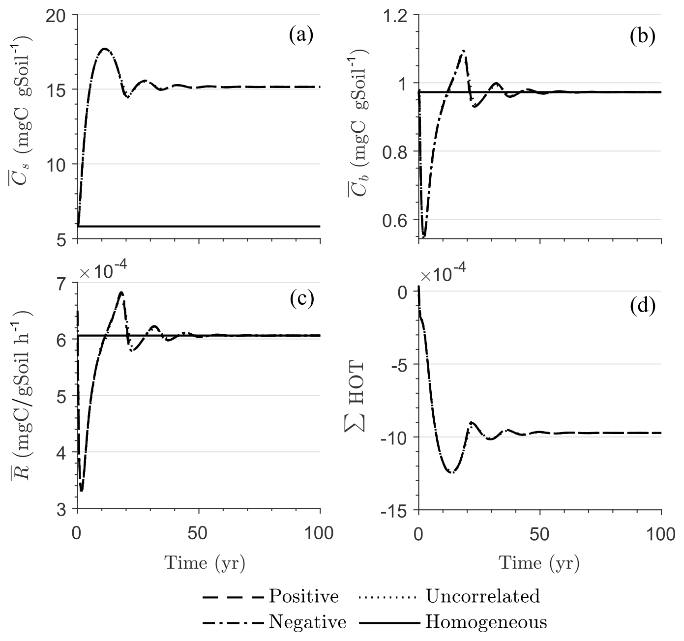
Figure A2(a) Mean substrate C (), (b) mean microbial C (), (c) mean respiration rate (), and (d) sum of second- and third-order terms (∑HOT) are shown as a function of time for different scenarios of initial spatial heterogeneity. This figure is similar to Fig. 4 for the full heterogeneity case, but with increased heterogeneity of the rate constant (kM).
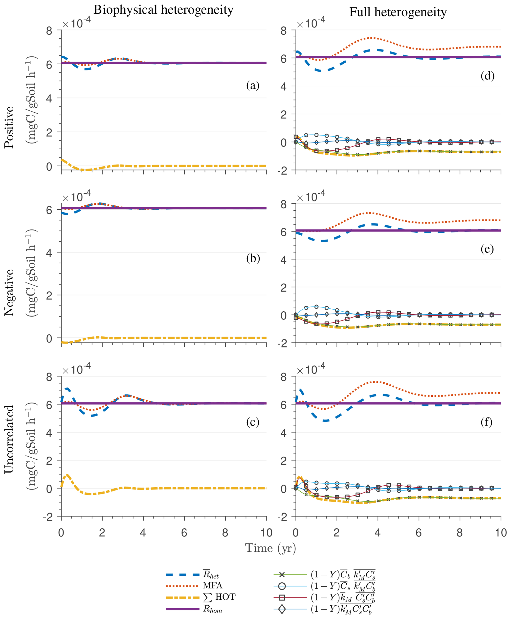
Figure A3Scenario 1 (steady-state simulation): temporal evolution of mean respiration rate in the heterogeneous system (, including the mean field approximation (MFA) and second-order terms) and the respiration rate in the homogeneous system () for multiplicative kinetics and for (a–c) the biophysical and (d–f) the fully heterogeneous system with (a–d) positively and (b–e) negatively correlated or (c–f) uncorrelated initial substrate and microbial C.
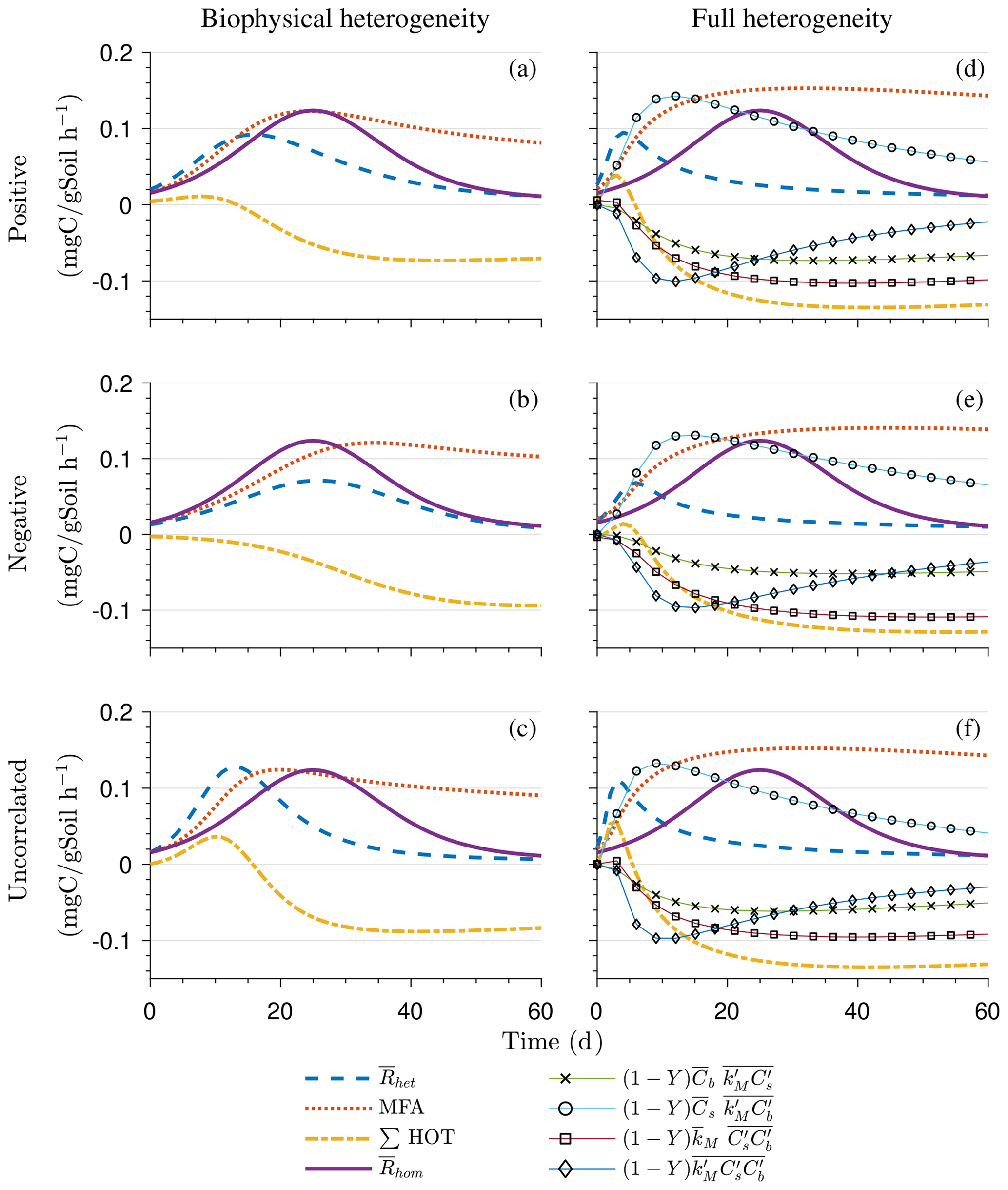
Figure A4Scenario 2 (HS simulation with multiplicative kinetics): temporal evolution of mean respiration rate in the heterogeneous system (), which includes the mean field approximation (MFA) and second-order terms, and the respiration rate in the homogeneous system () for (a–c) the biophysically and (d–f) the fully heterogeneous system with positive (a–b), negative (c–d), and uncorrelated (e–f) substrate and microbial C for multiplicative kinetics.
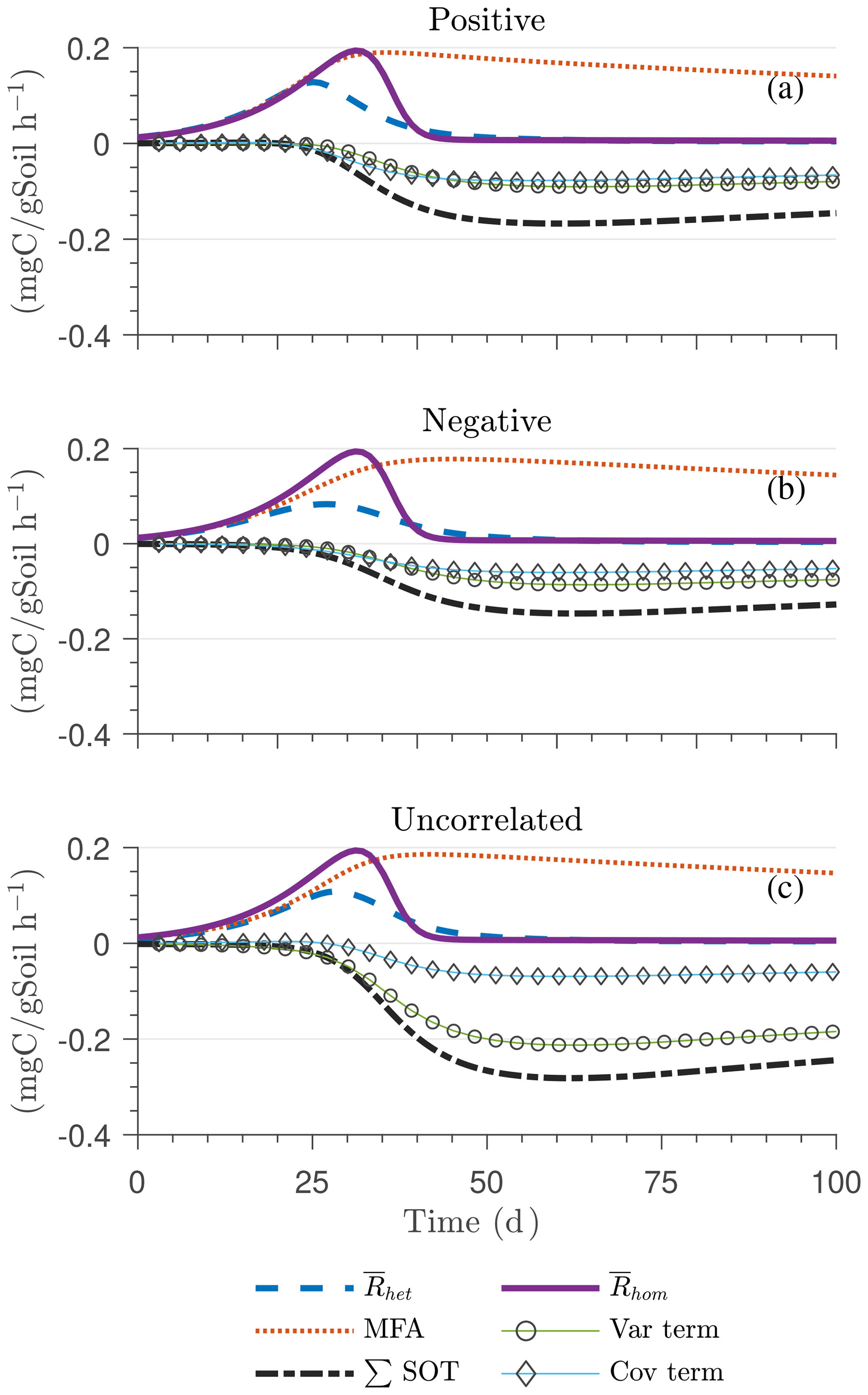
Figure A5Scenario 2 (HS with Michaelis–Menten kinetics): temporal evolution of mean respiration rate in the biophysically heterogeneous system (, including the mean field approximation (MFA) and second-order terms) and the respiration rate in the homogeneous system () for (a) positively and (b) negatively correlated or (c) uncorrelated substrate and microbial C.

Figure A6Scenario 2 (HS with inverse Michaelis–Menten kinetics): temporal evolution of mean respiration rate in the biophysically heterogeneous system (, including the mean field approximation (MFA) and second-order terms) and the respiration rate in the homogeneous system () for (a) positively and (b) negatively correlated or (c) uncorrelated substrate and microbial C.
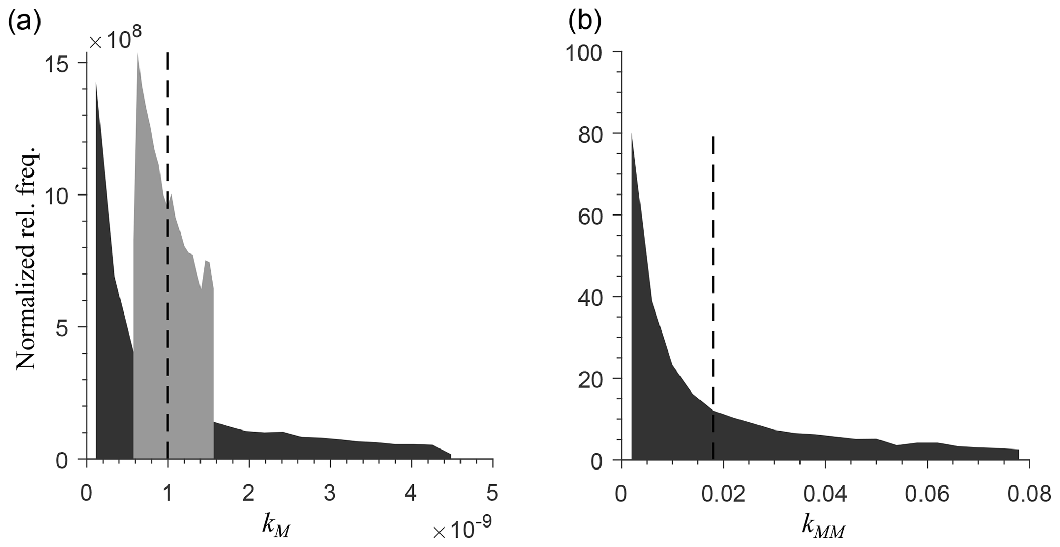
Figure A7Distribution of the decomposition rate constant for different degrees of biochemical heterogeneity and for (a) multiplicative and (b) Michaelis–Menten kinetics. Black and grey shading represents a higher and lower degree of biochemical heterogeneity, respectively, and the dashed line represents the mean rate constant for the homogeneous system. The half-saturation constant KMM is uniformly distributed; not shown in figure.
Table A2Initial mean substrate and microbial C in scenarios SS and HS, expressed in both femtograms of carbon (fg C) per grid cell and milligrams of carbon per gram of soil (values in brackets).
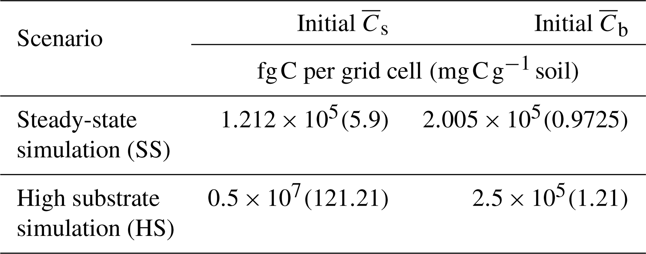
Table A3Probability distributions of the parameters for the multiplicative, MM, and IMM kinetics models. Values in brackets indicate the minimum and maximum parameter values.
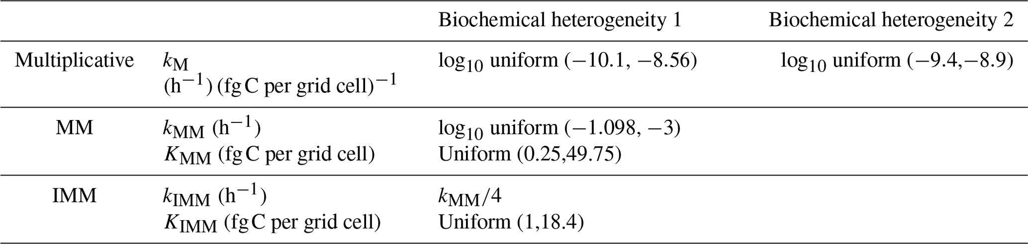
The article is based on synthetic data generated by the code described under “Code availability”.
All authors conceived the initial conceptualization. Arjun Chakrawal and Stefano Manzoni developed the theoretical formalism and performed the analytic calculations. Arjun Chakrawal performed the numerical simulations and led the writing of the paper. All authors discussed the results, provided critical feedback, and revised the paper.
The authors declare that they have no conflict of interest.
The authors would like to thank Thomas Wutzler, Ali Ebrahimi, and an anonymous reviewer for their insightful comments.
This research has been supported by the Vetenskapsrådet (grant no. 2016-04146) and the Svenska Forskningsrådet Formas (grant no. 2015-468).
The article processing charges for this open-access
publication were covered by Stockholm University.
This paper was edited by Wolfgang Kurtz and reviewed by Thomas Wutzler, Ali Ebrahimi, and one anonymous referee.
Abramoff, R., Xu, X., Hartman, M., O’Brien, S., Feng, W., Davidson, E., Finzi, A., Moorhead, D., Schimel, J., Torn, M., and Mayes, M. A.: The Millennial model: in search of measurable pools and transformations for modeling soil carbon in the new century, Biogeochemistry, 137, 51–71, https://doi.org/10.1007/s10533-017-0409-7, 2018. a
Albertson, J. D. and Montaldo, N.: Temporal dynamics of soil moisture variability: 1. Theoretical basis, Water Resour. Res., 39, 1–14, https://doi.org/10.1029/2002WR001616, 2003. a
Aleklett, K., Kiers, E. T., Ohlsson, P., Shimizu, T. S., Caldas, V. E., and Hammer, E. C.: Build Your Own Soil: Exploring Microfluidics to Create Microbial Habitat Structures, ISME J., 12, 312–319, https://doi.org/10.1038/ismej.2017.184, 2018. a
Allison, S. D.: Cheaters, diffusion and nutrients constrain decomposition by microbial enzymes in spatially structured environments, Ecol. Lett., 8, 626–635, https://doi.org/10.1111/j.1461-0248.2005.00756.x, 2005. a
Allison, S. D.: A trait-based approach for modelling microbial litter decomposition, Ecol. Lett., 15, 1058–1070, https://doi.org/10.1111/j.1461-0248.2012.01807.x, 2012. a
Barraquand, F. and Murrell, D. J.: Scaling up predator-prey dynamics using spatial moment equations, Meth. Ecol. Evol., 4, 276–289, https://doi.org/10.1111/2041-210X.12014, 2013. a, b
Bergström, U., Englund, G., and Leonardsson, K.: Plugging space into predator-prey models: an empirical approach., Am. Nat., 167, 246–259, https://doi.org/10.1086/499372, 2006. a, b, c
Bouckaert, L., Sleutel, S., Van Loo, D., Brabant, L., Cnudde, V., Van Hoorebeke, L., and De Neve, S.: Carbon mineralisation and pore size classes in undisturbed soil cores, Soil Res., 51, 14–22, https://doi.org/10.1071/SR12116, 2013. a
Chakrawal, A.: Dynamic upscaling of decomposition kinetics for carbon cycling models: Heterogeneous_SOMDynamics-v2.0, https://doi.org/10.5281/zenodo.3576613, 2019. a
Chesson, P.: Making sense of spatial models in ecology, Modeling spatiotemporal dynamics in ecology, Landes Bioscience Austin, Texas, USA, 151–166, 1998. a
Dagan, G.: Theory of solute transport by groundwater, Annu. Rev. Fluid Mech., 19, 183–213, https://doi.org/10.1146/annurev.fl.19.010187.001151, 1987. a
Dentz, M., Le Borgne, T., Englert, A., and Bijeljic, B.: Mixing, spreading and reaction in heterogeneous media: A brief review, J. Contam. Hydrol., 120–121, 1–17, https://doi.org/10.1016/j.jconhyd.2010.05.002, 2011. a, b
Don, A., Rödenbeck, C., and Gleixner, G.: Unexpected control of soil carbon turnover by soil carbon concentration, Environ. Chem. Lett., 11, 407–413, 2013. a, b
Dungait, J. A., Hopkins, D. W., Gregory, A. S., and Whitmore, A. P.: Soil organic matter turnover is governed by accessibility not recalcitrance, Glob. Change Biol., 18, 1781–1796, https://doi.org/10.1111/j.1365-2486.2012.02665.x, 2012. a
Ebrahimi, A. and Or, D.: Microbial community dynamics in soil aggregates shape biogeochemical gas fluxes from soil profiles – upscaling an aggregate biophysical model, Glob. Change Biol., 22, 3141–3156, https://doi.org/10.1111/gcb.13345, 2016. a
Ebrahimi, A. and Or, D.: On Upscaling of Soil Microbial Processes and Biogeochemical Fluxes From Aggregates to Landscapes, J. Geophys. Res.-Biogeo., 123, 1526–1547, https://doi.org/10.1029/2017JG004347, 2018. a
Ekschmitt, K., Kandeler, E., Poll, C., Brune, A., Buscot, F., Friedrich, M., Gleixner, G., Hartmann, A., Kästner, M., Marhan, S., Miltner, A., Scheu, S., and Wolters, V.: Soil-carbon preservation through habitat constraints and biological limitations on decomposer activity, J. Plant Nutr. Soil Sc., 171, 27–35, https://doi.org/10.1002/jpln.200700051, 2008. a
Englund, G. and Leonardsson, K.: Scaling up the functional response for spatially heterogeneous systems, Ecol. Lett., 11, 440–449, https://doi.org/10.1111/j.1461-0248.2008.01159.x, 2008. a
Falconer, R. E., Battaia, G., Schmidt, S., Baveye, P., Chenu, C., and Otten, W.: Microscale Heterogeneity Explains Experimental Variability and Non-Linearity in Soil Organic Matter Mineralisation, PLOS ONE, 10, e0123774, https://doi.org/10.1371/journal.pone.0123774, 2015. a, b
Fatichi, S., Katul, G. G., Ivanov, V. Y., Pappas, C., Paschalis, A., Consolo, A., Kim, J., and Burlando, P.: Abiotic and biotic controls of soil moisture spatiotemporal variability and the occurrence of hysteresis, Water Resour. Res., 51, 3505–3524, https://doi.org/10.1002/2014WR016102, 2015. a
Forney, D. C. and Rothman, D. H.: Common structure in the heterogeneity of plant-matter decay, J. R. Soc. Interface, 9, 2255–2267, https://doi.org/10.1098/rsif.2012.0122, 2012. a, b
Fraser, F. C., Todman, L. C., Corstanje, R., Deeks, L. K., Harris, J. A., Pawlett, M., Whitmore, A. P., and Ritz, K.: Distinct respiratory responses of soils to complex organic substrate are governed predominantly by soil architecture and its microbial community, Soil Biol. Biochem. 103, 493–501, https://doi.org/10.1016/j.soilbio.2016.09.015, 2016. a
Georgiou, K., Abramoff, R. Z., Harte, J., Riley, W. J., and Torn, M. S.: Microbial community-level regulation explains soil carbon responses to long-term litter manipulations, Nat. Commun., 8, 1–10, https://doi.org/10.1038/s41467-017-01116-z, 2017. a
German, D. P., Marcelo, K. R. B., Stone, M. M., and Allison, S. D.: The Michaelis-Menten kinetics of soil extracellular enzymes in response to temperature: A cross-latitudinal study, Glob. Change Biol., 18, 1468–1479, https://doi.org/10.1111/j.1365-2486.2011.02615.x, 2012. a
Ginovart, M. and Valls, J.: Individual Based Modelling of Microbial Activity to Study Mineralization and Nitrification Process in Soil, AICME II abstracts, 6, 773–795, https://doi.org/10.1016/j.nonrwa.2004.12.005, 1996. a
Herbst, M., Tappe, W., Kummer, S., and Vereecken, H.: The impact of sieving on heterotrophic respiration response to water content in loamy and sandy topsoils, Geoderma, 272, 73–82, https://doi.org/10.1016/j.geoderma.2016.03.002, 2016. a, b
Hunt, A. G. and Manzoni, S.: Networks on Networks, 2053–2571, Morgan & Claypool Publishers, 175 pp., https://doi.org/10.1088/978-1-6817-4159-8, 2015. a
Jenkinson, D. and Rayner, J.: The turnover of soil organic matter in some of the Rothamsted classical experiments, Soil Sci., 123, 298–305, 1977. a
Jenny, H., Gessel, S., and Bingham, F.: Comparative study of decomposition rates of organic matter in temperate and tropical regions, Soil Sci., 68, 419–432, 1949. a
Juarez, S., Nunan, N., Duday, A. C., Pouteau, V., Schmidt, S., Hapca, S., Falconer, R., Otten, W., and Chenu, C.: Effects of different soil structures on the decomposition of native andadded organic carbon, Eur. J. Soil Biol., 58, 81–90, https://doi.org/10.1016/j.ejsobi.2013.06.005, 2013. a, b
Kaiser, C., Franklin, O., Dieckmann, U., and Richter, A.: Microbial community dynamics alleviate stoichiometric constraints during litter decay, Ecol. Lett., 17, 680–690, https://doi.org/10.1111/ele.12269, 2014. a, b
Keeling, M. J. J., Wilson, H. B. B., and Pacala, S. W. W.: Deterministic Limits to Stochastic Spatial Models of Natural Enemies, Am. Nat., 159, 57–80, https://doi.org/10.1086/324119, 2002. a
Keiluweit, M., Wanzek, T., Kleber, M., Nico, P., and Fendorf, S.: Anaerobic microsites have an unaccounted role in soil carbon stabilization, Nat. Commun., 8, 1771, https://doi.org/10.1038/s41467-017-01406-6, 2017. a
Killham, K., Amato, M., and Ladd, J. N.: Effect of substrate location in soil and soil pore-water regime on carbon turnover, Soil Biol. Biochem., 25, 57–62, https://doi.org/10.1016/0038-0717(93)90241-3, 1993. a, b
Koestel, J. and Schlüter, S.: Quantification of the structure evolution in a garden soil over the course of two years, Geoderma, 338, 597–609, https://doi.org/10.1016/j.geoderma.2018.12.030, 2019. a
Kravchenko, A. N. and Guber, A. K.: Soil pores and their contributions to soil carbon processes, Geoderma, 287, 31–39, https://doi.org/10.1016/j.geoderma.2016.06.027, 2017. a, b
Kuzyakov, Y. and Blagodatskaya, E.: Microbial hotspots and hot moments in soil: concept & review, Soil Biol. Biochem., 83, 184–199, https://doi.org/10.1016/j.soilbio.2015.01.025, 2015. a
Lennon, J. J.: Red-shifts and red herrings in geographical ecology, Ecography, 23, 101–113, https://doi.org/10.1111/j.1600-0587.2000.tb00265.x, 2000. a
Lugo-Méndez, H. D., Valdés-Parada, F. J., Porter, M. L., Wood, B. D., and Ochoa-Tapia, J. A.: Upscaling Diffusion and Nonlinear Reactive Mass Transport in Homogeneous Porous Media, Transport Porous Med., 107, 683–716, https://doi.org/10.1007/s11242-015-0462-4, 2015. a
Manzoni, S. and Katul, G.: Invariant soil water potential at zero microbial respiration explained by hydrological discontinuity in dry soils, Geophys. Res. Lett., 41, 7151–7158, https://doi.org/10.1002/2014GL061467, 2014. a
Manzoni, S. and Porporato, A.: A theoretical analysis of nonlinearities and feedbacks in soil carbon and nitrogen cycles, Soil Biol. Biochem., 39, 1542–1556, https://doi.org/10.1016/j.soilbio.2007.01.006, 2007. a, b, c
Manzoni, S. and Porporato, A.: Soil carbon and nitrogen mineralization: Theory and models across scales, Soil Biol. Biochem., 41, 1355–1379, https://doi.org/10.1016/j.soilbio.2009.02.031, 2009. a, b, c, d
Manzoni, S., Porporato, A., and Schimel, J. P.: Soil heterogeneity in lumped mineralization–immobilization models, Soil Biol. Biochem., 40, 1137–1148, https://doi.org/10.1016/j.soilbio.2007.12.006, 2008. a, b
Manzoni, S., Piñeiro, G., Jackson, R. B., Jobbágy, E. G., Kim, J. H., and Porporato, A.: Analytical models of soil and litter decomposition: Solutions for mass loss and time-dependent decay rates, Soil Biol. Biochem., 50, 66–76, https://doi.org/10.1016/j.soilbio.2012.02.029, 2012. a
Melbourne, B. A. and Chesson, P.: The scale transition: Scaling up population dynamics with field data, Ecology, 87, 1478–1488, https://doi.org/10.1890/0012-9658(2006)87[1478:TSTSUP]2.0.CO;2, 2006. a
Monga, O., Bousso, M., Garnier, P., and Pot, V.: 3D geometric structures and biological activity: Application to microbial soil organic matter decomposition in pore space, Ecol. Model., 216, 291–302, https://doi.org/10.1016/j.ecolmodel.2008.04.015, 2008. a
Monga, O., Garnier, P., Pot, V., Coucheney, E., Nunan, N., Otten, W., and Chenu, C.: Simulating microbial degradation of organic matter in a simple porous system using the 3-D diffusion-based model MOSAIC, Biogeosciences, 11, 2201–2209, https://doi.org/10.5194/bg-11-2201-2014, 2014. a
Morozov, A. and Poggiale, J. C.: From spatially explicit ecological models to mean-field dynamics: The state of the art and perspectives, Ecol. Compl., 10, 1–11, https://doi.org/10.1016/j.ecocom.2012.04.001, 2012. a
Murrell, D. J., Dieckmann, U., and Law, R.: On moment closures for population dynamics in continuous space, J. Theor. Biol. 229, 421–432, https://doi.org/10.1016/j.jtbi.2004.04.013, 2004. a
Negassa, W. C., Guber, A. K., Kravchenko, A. N., Marsh, T. L., Hildebrandt, B., and Rivers, M. L.: Properties of soil pore space regulate pathways of plant residue decomposition and community structure of associated bacteria, PLoS ONE, 10, 1–22, https://doi.org/10.1371/journal.pone.0123999, 2015. a
Nguyen-Ngoc, D., Leye, B., Monga, O., Garnier, P., and Nunan, N.: Modeling Microbial Decomposition in Real 3D Soil Structures Using Partial Differential Equations, Int. J. Geosci., 4, 15–26, https://doi.org/10.4236/ijg.2013.410A003, 2013. a
Nunan, N., Wu, K., Young, I. M., Crawford, J. W., and Ritz, K.: In situ spatial patterns of soil bacterial populations, mapped at multiple scales, in an arable soil, Microb. Ecol. 44, 296–305, https://doi.org/10.1007/s00248-002-2021-0, 2002. a
Nunan, N., Wu, K., Young, I. M., Crawford, J. W., and Ritz, K.: Spatial distribution of bacterial communities and their relationships with the micro-architecture of soil, FEMS Microbiol. Ecol., 44, 203–215, https://doi.org/10.1016/S0168-6496(03)00027-8, 2003. a
Olson, J. S.: Energy Storage and the Balance of Producers and Decomposers in Ecological Systems, Ecology, 44, 322–331, https://doi.org/10.2307/1932179, 1963. a
Parton, W., Schimel, D. S., Cole, C., and Ojima, D.: Analysis of factors controlling soil organic matter levels in Great Plains Grasslands 1, Soil Sci. Soc. Am. J., 51, 1173–1179, 1987. a
Peth, S., Chenu, C., Leblond, N., Mordhorst, A., Garnier, P., Nunan, N., Pot, V., Ogurreck, M., and Beckmann, F.: Localization of soil organic matter in soil aggregates using synchrotron-based X-ray microtomography, Soil Biol. Biochem., 78, 189–194, https://doi.org/10.1016/j.soilbio.2014.07.024, 2014. a
Porter, M. L., Valdés-Parada, F. J., and Wood, B. D.: Multiscale modeling of chemotaxis in homogeneous porous media, Water Resour. Res., 47, 1–13, https://doi.org/10.1029/2010WR009646, 2011. a
Rawlins, B. G., Wragg, J., Reinhard, C., Atwood, R. C., Houston, A., Lark, R. M., and Rudolph, S.: Three-dimensional soil organic matter distribution, accessibility and microbial respiration in macroaggregates using osmium staining and synchrotron X-ray computed tomography, SOIL, 2, 659–671, https://doi.org/10.5194/soil-2-659-2016, 2016. a, b
Raynaud, X. and Nunan, N.: Spatial ecology of bacteria at the microscale in soil, PLoS ONE, 9, e87217, https://doi.org/10.1371/journal.pone.0087217, 2014. a, b
Ruamps, L. S., Nunan, N., and Chenu, C.: Microbial biogeography at the soil pore scale, Soil Biol. Biochem., 43, 280–286, https://doi.org/10.1016/J.SOILBIO.2010.10.010, 2011. a, b
Salomé, C., Nunan, N., Pouteau, V., Lerch, T. Z., and Chenu, C.: Carbon dynamics in topsoil and in subsoil may be controlled by different regulatory mechanisms, Glob. Change Biol., 16, 416–426, https://doi.org/10.1111/j.1365-2486.2009.01884.x, 2010. a
Schimel, J. P. and Weintraub, M. N.: The implications of exoenzyme activity on microbial carbon and nitrogen limitation in soil: A theoretical model, Soil Biol. Biochem., 35, 549–563, https://doi.org/10.1016/S0038-0717(03)00015-4, 2003. a, b, c
Schmidt, M. W., Torn, M. S., Abiven, S., Dittmar, T., Guggenberger, G., Janssens, I. A., Kleber, M., Kögel-Knabner, I., Lehmann, J., Manning, D. A., Nannipieri, P., Rasse, D. P., Weiner, S., and Trumbore, S. E.: Persistence of soil organic matter as an ecosystem property, Nature, 478, 49–56, https://doi.org/10.1038/nature10386, 2011. a
Schnecker, J., Bowles, T., Hobbie, E. A., Smith, R. G., and Grandy, A. S.: Substrate quality and concentration control decomposition and microbial strategies in a model soil system, Biogeochemistry, 144, 47–59, https://doi.org/10.1007/s10533-019-00571-8, 2019. a, b
Sierra, C. A. and Muller, M.: A general mathematical framework for representing soil organic matter dynamics, Ecol. Monogr. 85, 505–524, https://doi.org/10.1890/15-0361.1, 2015. a, b
Stanley, C. E., Grossmann, G., i Solvas, X. C., and deMello, A. J.: Soil-on-a-Chip: Microfluidic Platforms for Environmental Organismal Studies, Lab Chip, 16, 228–241, https://doi.org/10.1039/C5LC01285F, 2016. a
Stenger, R., Barkle, G. F., and Burgess, C. P.: Mineralisation of organic matter in intact versus sieved/refilled soil cores, Soil Res., 40, 149–160, https://doi.org/10.1071/SR01003, 2002. a
Tang, J. Y. and Riley, W. J.: A total quasi-steady-state formulation of substrate uptake kinetics in complex networks and an example application to microbial litter decomposition, Biogeosciences, 10, 8329–8351, https://doi.org/10.5194/bg-10-8329-2013, 2013. a, b
Tang, J.-Y. and Riley, W. J.: SUPECA kinetics for scaling redox reactions in networks of mixed substrates and consumers and an example application to aerobic soil respiration, Geosci. Model Dev., 10, 3277–3295, https://doi.org/10.5194/gmd-10-3277-2017, 2017. a, b, c
Valdés-Parada, F. J., Porter, M. L., Narayanaswamy, K., Ford, R. M., and Wood, B. D.: Upscaling microbial chemotaxis in porous media, Adv. Water Resour., 32, 1413–1428, https://doi.org/10.1016/j.advwatres.2009.06.010, 2009. a
Van Oijen, M., Cameron, D., Levy, P. E., and Preston, R.: Correcting errors from spatial upscaling of nonlinear greenhouse gas flux models, Environ. Model. Softw., 94, 157–165, https://doi.org/10.1016/j.envsoft.2017.03.023, 2017. a, b, c
Wang, B. and Allison, S. D.: Emergent properties of organic matter decomposition by soil enzymes, Soil Biol. Biochemistry, 136, 107522, https://doi.org/10.1016/j.soilbio.2019.107522, 2019. a
Watt, M., Silk, W. K., and Passioura, J. B.: Rates of root and organism growth, soil conditions, and temporal and spatial development of the rhizosphere, Ann. Bot., 97, 839–855, https://doi.org/10.1093/aob/mcl028, 2006. a, b
Whitaker, S.: The Method of Volume Averaging, vol. 13, Theory and Applications of Transport in Porous Media, Springer Netherlands, Dordrecht, https://doi.org/10.1007/978-94-017-3389-2, 1999. a
Wieder, W. R., Bonan, G. B., and Allison, S. D.: Global soil carbon projections are improved by modelling microbial processes, Nat. Clim. Change, 3, 909–912, https://doi.org/10.1038/nclimate1951, 2013. a
Wieder, W. R., Allison, S. D., Davidson, E. A., Georgiou, K., Hararuk, O., He, Y., Hopkins, F., Luo, Y., Smith, M. J., Sulman, B., Todd-Brown, K., Wang, Y. P., Xia, J., and Xu, X.: Explicitly representing soil microbial processes in Earth system models, Global Biogeochem. Cy., 29, 1782–1800, https://doi.org/10.1002/2015GB005188, 2015. a, b
Wieder, W. R., Hartman, M. D., Sulman, B. N., Wang, Y. P., Koven, C. D., and Bonan, G. B.: Carbon cycle confidence and uncertainty: Exploring variation among soil biogeochemical models, Glob. Change Biol., 24, 1563–1579, https://doi.org/10.1111/gcb.13979, 2018. a, b
Witter, E.: Soil C balance in a long-term field experiment in relation to the size of the microbial biomass, Biol. Fert. Soils, 23, 33–37, https://doi.org/10.1007/BF00335815, 1996. a
Wutzler, T. and Reichstein, M.: Colimitation of decomposition by substrate and decomposers – a comparison of model formulations, Biogeosciences, 5, 749–759, https://doi.org/10.5194/bg-5-749-2008, 2008. a
Xie, X. S.: Enzyme Kinetics, Past and Present, Science, 342, 1457–1459, https://doi.org/10.1126/science.1248859, 2013. a
Xu, X., Thornton, P. E., and Post, W. M.: A global analysis of soil microbial biomass carbon, nitrogen and phosphorus in terrestrial ecosystems, Global Ecol. Biogeogr., 22, 737–749, 2013. a
Yan, Z., Liu, C., Todd-Brown, K. E., Liu, Y., Bond-Lamberty, B., and Bailey, V. L.: Pore-scale investigation on the response of heterotrophic respiration to moisture conditions in heterogeneous soils, Biogeochemistry, 131, 121–134, https://doi.org/10.1007/s10533-016-0270-0, 2016. a
Zelenev, V., Bruggen, A. V., and Semenov, A.: BACWAVE, a Spatial–Temporal Model for Traveling Waves of Bacterial Populations in Response to a Moving Carbon Source in Soil, Microb. ecol., 40, 260–272, https://doi.org/10.1007/s002480000029, 2000. a, b