the Creative Commons Attribution 4.0 License.
the Creative Commons Attribution 4.0 License.
 | 22 Feb 2019
The Cloud_cci simulator v1.0 for the Cloud_cci climate data record and its application to a global and a regional climate model
Salomon Eliasson
Karl Göran Karlsson
Erik van Meijgaard
Jan Fokke Meirink
Martin Stengel
Ulrika Willén
The Cloud Climate Change Initiative (Cloud_cci) satellite simulator has been developed to enable comparisons between the Cloud_cci climate data record (CDR) and climate models. The Cloud_cci simulator is applied here to the EC-Earth global climate model as well as the Regional Atmospheric Climate Model (RACMO) regional climate model. We demonstrate the importance of using a satellite simulator that emulates the retrieval process underlying the CDR as opposed to taking the model output directly. The impact of not sampling the model at the local overpass time of the polar-orbiting satellites used to make the dataset was shown to be large, yielding up to 100 % error in liquid water path (LWP) simulations in certain regions. The simulator removes all clouds with optical thickness smaller than 0.2 to emulate the Cloud_cci CDR's lack of sensitivity to very thin clouds. This reduces total cloud fraction (TCF) globally by about 10 % for EC-Earth and by a few percent for RACMO over Europe. Globally, compared to the Cloud_cci CDR, EC-Earth is shown to be mostly in agreement on the distribution of clouds and their height, but it generally underestimates the high cloud fraction associated with tropical convection regions, and overestimates the occurrence and height of clouds over the Sahara and the Arabian subcontinent. In RACMO, TCF is higher than retrieved over the northern Atlantic Ocean but lower than retrieved over the European continent, where in addition the cloud top pressure (CTP) is underestimated. The results shown here demonstrate again that a simulator is needed to make meaningful comparisons between modeled and retrieved cloud properties. It is promising to see that for (nearly) all cloud properties the simulator improves the agreement of the model with the satellite data.
- Article
(12422 KB) - Full-text XML
- BibTeX
- EndNote


Clouds have a critical impact on the Earth's radiative budget and its hydrological cycle, yet clouds also present the largest source of uncertainties in climate models (Zelinka et al., 2017). Therefore, in order to increase the fidelity of a model's ability to predict a future climate, a realistic representation of clouds is needed. Indeed, for decades, the representation of clouds in models has improved to the degree that we can now make confident statements on the overall cloud-feedback response to a changing climate (Klein et al., 2013; Zelinka et al., 2017). This improvement has for a considerable part been enabled by the increased availability of global satellite measurements of clouds. However, despite great strides having been made in improving the representation of clouds since the Intergovernmental Panel on Climate Change (IPCC)'s First Assessment Report, they still constitute one of the main challenges to climate modeling (IPCC, 2014).
More than 30 years ago, to improve weather forecasts, operational weather satellites were launched to monitor the atmosphere and surface. Thanks to their strategic importance, these satellites have been, and still are being, replaced at the end of their mission. Several cloud climate data records (CDRs) have made use of the long-term data continuity from these satellites, and together they have greatly enhanced our understanding of climate. There are several satellite CDRs based on more than 30 years worth of passive measurements including the International Satellite Cloud Climatology Project (ISCCP) (Young et al., 2018), Pathfinder Atmospheres – Extended (PATMOS-x) (Heidinger et al., 2014), Satellite Application Facility on Climate Monitoring (CM SAF) cLoud, Albedo and RAdiation dataset (CLARA)-A2 (Karlsson et al., 2017), and the CDR this paper concerns, Cloud Climate Change Initiative (Cloud_cci) Advanced Very High Resolution Radiometer (AVHRR)-PM v2.0 (Stengel et al., 2017).
All these long-term CDRs have very good spatial coverage and are sufficiently long to capture naturally occurring interannual cycles such as El Niño–Southern Oscillation (ENSO) and to detect potential climate change signals that emerge from the internal variability (noise) inherent to the climate system. They all have their strengths and weaknesses. For example, ISCCP is well suited for assessing the diurnal cycle of clouds because it uses measurements from geostationary satellites. The other aforementioned data records make use of the spectrally more resolved information from the polar-orbiting AVHRR instrument, allowing the retrieval of a wider range of cloud products with presumably higher accuracy.
The Cloud_cci CDR (except its cloud mask and phase identification) has been retrieved using the optimal estimation technique. All cloud properties are radiatively consistent with each other since they were retrieved simultaneously using visible and thermal infrared channel measurements. One general benefit to the optimal estimation technique is that uncertainties in a priori estimates and other input data will be propagated, and therefore uncertainty estimates are also retrieved together with the solution. The uncertainty retrievals, which provide the modeled random error in the retrieval, are useful since they provide a guide in identifying the CDR's strengths and weaknesses. However, a user still needs to be mindful of systematic errors in retrievals (biases), which are not reported despite often being the most serious source of retrieval error. Systematic errors in retrievals are often heavily situation dependent and can only be estimated by validation against bias-free reference observations.
Other CDRs from passive imagers, such as the MODerate resolution Imaging Spectroradiometer (MODIS), Advanced Along-Track Scanning Radiometer (AATSR), Multi-angle Imaging SpectroRadiometer (MISR), also provide global cloud products but these satellites are research missions and are not expected to be replaced and have not been around for as long as the AVHRR-based CDRs, so the corresponding data records are shorter and therefore less suitable for climate studies. However, these CDRs are also very valuable since they are based on retrievals from more advanced instruments which measure at more wavelengths and therefore generally can provide arguably even better cloud retrievals.
Since 2006, climate model developers have made great use of measurements from the satellite-borne active Cloud-Aerosol Lidar with Orthogonal Polarization (CALIOP) (Winker et al., 2009) and CloudSat (Stephens et al., 2002) instruments. These measure the vertical distribution of clouds and the lidar has a much stronger sensitivity to thin clouds than measurements from (nadir-looking) passive instruments, such as those mentioned earlier. The CDRs from these active instruments have immensely improved our understanding of the vertical structure of clouds and their occurrence in general. They have also been used to constrain the vertical distribution of clouds and their impact on the radiation budget in models. CALIOP and CloudSat data have also served as very accurate references for validating and improving passive-imager-based cloud retrievals (e.g., Stengel et al., 2015; Karlsson and Håkansson, 2018).
When these CDRs are used for the evaluation of (climate) models, it is important to realize that, in general modeled clouds cannot be directly compared to satellite-derived CDRs. In the models, clouds are represented as bulk properties on grids ranging from on the order of 10 km for regional models to 100 km for global models, while the observations are made by instruments that typically measure at much smaller scales. The sensitivity of satellite retrievals to clouds also strongly depends on the wavelength at which the measurements are being made as well as the type of cloud that is being observed (Waliser et al., 2009). On top of this, clouds are represented on a three-dimensional spatial grid in models, whereas retrievals based on passive visible and infrared instruments, like the Cloud_cci CDR, do not yield vertically resolved information on clouds but rather cloud top and column-integrated cloud properties. Therefore, to assess modeled cloudiness against observations, these and more factors should be taken into account in order to make the modeled and satellite-retrieved clouds comparable.
This notion led to the development of so-called satellite simulators. Jakob and Klein (1999) described the first satellite product simulator for the ISCCP CDR. The use of the ISCCP simulator was demonstrated in a model evaluation in Webb et al. (2001). Since then, several studies using the ISCCP simulator were made in an effort to constrain modeled clouds, and good progress was made (e.g., Norris et al., 2016; Terai et al., 2016; Tan et al., 2017).
Following the initial developments for ISCCP, many other cloud property satellite simulators have been established for a range of instruments. Simulators for passive visible–infrared imagers include the MODIS simulator by Pincus et al. (2012) and Spinning Enhanced Visible and Infrared Imager (SEVIRI) simulators by Bugliaro et al. (2011) and Jonkheid et al. (2012). (The latter reference also provides a conceptual framework of cloud simulators in general and their role in model evaluation.) QuickBeam simulates the vertical profile of clouds that would have been measured by the satellite-borne cloud radar CloudSat, if the model atmosphere was the real atmosphere (Haynes et al., 2007). Similarly, a simulator of lidar data was developed for comparison with the Cloud-Aerosol Lidar and Infrared Pathfinder Satellite Observation (CALIPSO) CDR as described in Chepfer et al. (2008). The simulator for Earth Clouds, Aerosol and Radiation Explorer (EarthCARE) called ECSIM (Voors et al., 2007) simulates the instruments in the EarthCARE mission, targeting small-scale cloud fields in particular.
A range of these satellite simulators has been gathered into a simulator package called Cloud Feedback Model Intercomparison Project (CFMIP) Observation Simulator Package (COSP) (Bodas-Salcedo et al., 2011; Swales et al., 2018), which is now considered an indispensable tool for assessing the representation of clouds in climate models. Particularly since there are several different flavors of satellite CDR simulators in COSP, a user can use different simulators to address different aspects of a model (Kay et al., 2012; Webb et al., 2017; Song et al., 2017). The COSP is a self-contained software package that requires model input of vertical cloud, temperature, and humidity data. COSP can be installed into a model code, so that simulated observational data can be generated and saved together with other model fields. However, COSP can also be used “offline” on archived model data. The main advantage of running COSP integrated into the models' own software environment is to avoid storing large volumes of data otherwise needed for running the simulators afterwards. The disadvantage of installing COSP into a model is that, when installed in the model, runtime is considerably increased (Norris et al., 2016).
Here, we present the Cloud_cci satellite product simulator that emulates the Cloud_cci CDR so that climate modelers can make full use of this new CDR and its advantages. This simulator is not yet a part of COSP but will be included in a branch on the COSP GitHub (https://github.com/CFMIP/COSPv2.0, last access: 12 February 2019) so that anyone who downloads this publicly available package will automatically have access to this simulator. The usefulness of the Cloud_cci simulator is demonstrated by applying it for an evaluation of the EC-Earth global climate model (GCM) (Hazeleger et al., 2010) and the Regional Atmospheric Climate Model (RACMO) (van Meijgaard et al., 2012) regional climate model (RCM).
The structure of this paper is as follows: the EC-Earth and RACMO models are described in Sect. 2.1 and 2.2, respectively, while the satellite Cloud_cci CDR is outlined in Sect. 2.3. The simulator proposed in this paper is presented in detail in Sect. 3. Results from applying the satellite simulator to EC-Earth and RACMO are given in Sects. 4 and 5, respectively. Finally, the results are summarized in Sect. 6.
2.1 Global climate model: EC-Earth
EC-Earth is a global climate system model. Its atmospheric part is based on the Integrated Forecast System (IFS) of the European Centre for Medium-Range Weather Forecasts (ECMWF) model. The version used in this study, EC-Earth3.2beta (Boussetta et al., 2016), is based on IFS cy36r4 in addition to a few important physical adjustments mainly related to the non-orographic gravity wave drag parameterization (latitudinal and resolution dependency of the launch momentum flux) and the diurnal cycle of convection (Bechtold et al., 2014).
To reproduce present-day climate variability, EC-Earth was run with prescribed observed sea surface temperature and sea ice using European reanalysis (ERA)-Interim monthly data as the lower boundary condition, according to the Atmospheric Model Intercomparison Project (AMIP) protocol. EC-Earth was run with a horizontal resolution of 70 km and on 91 vertical levels. The simulator will be installed in EC-Earth by including the simulator in COSP, but for this experiment the full model vertical fields were stored every 6 h and the model parameterization formulas for cloud overlap and particle effective radius were used to reproduce the in-model variables needed for the simulator.
The satellite-simulated cloud variables were compared with the Cloud_cci AVHRR-PM L3C data record, described in Sect. 2.3, after being aggregated to match the model resolution.
2.2 Regional climate model: RACMO
The hydrostatic RCM RACMO2 (van Meijgaard et al., 2012) was originally built from the parameterization package of physical processes employed in the ECMWF IFS model merged with the dynamical kernel of the High Resolution Limited Area Model (HIRLAM) (Unden et al., 2002) numerical weather prediction model. RACMO2.3 is used in this study. It is based on ECMWF IFS cy33r2, which constitutes large overlaps with the ECMWF physics of cy36r4 used in EC-Earth3.2 as described in Sect. 2.1.
Other physics components include a turbulence kinetic energy (TKE)-driven eddy-diffusivity mass-flux scheme (Siebesma et al., 2007; Lenderink and Holtslag, 2004) for mixing and cloud processes in the boundary layer, a scheme for deep convection (originated by Tiedtke, 1989), a prognostic cloud scheme (Tiedtke, 1993; Tompkins et al., 2007), and the land surface/soil scheme Hydrology Tiled ECMWF Scheme for Surface Exchanges over Land (TESSEL) (HTESSEL) (Balsamo et al., 2009). A rapid radiation transfer module (RRTM) accounts for solar (Clough et al., 2005) and terrestrial radiation (Mlawer et al., 1997). The effect of clouds on radiation at the subgrid scale is represented by the independent column approximation (ICA; Morcrette et al., 2008).
In the past years, RACMO has been frequently used in transient climate simulations with different GCM drivers (EC-Earth, Hadley Centre Global Environmental Model (HadGEM)2-ES) in the framework of the Coordinated Regional Climate Downscaling Experiment (CORDEX) (Giorgi and Gutowski, 2015) and in preparation of the KNMI'14 climate scenarios for the Netherlands (van den Hurk et al., 2014).
For this study, integrations with RACMO were carried out for the years 2011 to 2014 at a 25 km horizontal resolution and 40 model levels using a hybrid vertical coordinate. The model domain, configured by employing a rotated pole coordinate, roughly encompasses the region between 30∘ W to 50∘ E, and between 30 and 70∘ N. The integrations were driven by ERA-Interim atmospheric fields at the lateral boundaries and temperature and sea-ice extent at the sea surface. They were carried out in hindcast mode (instead of climate mode) implying short-term runs of 36 h. In the chosen setup, runs were re-initialized daily at 12:00 UTC from ERA-Interim including the land surface state.
To avoid effects from spinup, in particular in the cloud fields, the first 12 h of each run were not considered in the further processing. In this way, a quasi-continuous long-term time series of non-overlapping model output was constructed. The benefit of employing hindcast mode rather than climate mode is that the model atmospheric state stays close to the quasi-observed large-scale flow imposed by ERA-Interim, facilitating the comparison of the simulated cloud parameters with those inferred from satellite observations. Multi-level output, including cloud parameters like instantaneous cloud fraction, cloud liquid water content and cloud ice content, was archived in 3-hourly resolved files. The Cloud_cci simulator was then applied to this model output on the native RACMO grid.
Simulated model results were compared with the Cloud_cci CDR (see Sect. 2.3), which was aggregated to 25 km resolution in order to match the model resolution. Observed ice cloud fraction and liquid water cloud fraction were calculated from the number of 0.5∘ pixels indicating ice and liquid water clouds, respectively, in the designated 25 km cell. The aggregation of remaining cloud parameters was carried out accordingly.
2.3 The Cloud_cci CDR
For this study, we use the Cloud_cci AVHRR-PM v2.0 CDR, which contains cloud properties retrieved from global AVHRR observations from the afternoon satellites of the National Oceanic and Atmospheric Administration (NOAA) Earth Observing System (EOS) mission NOAA-7, 9, 11, 14, 16, 18, 19 (Stengel et al., 2017). Created with the Community Cloud Retrieval for Climate (CC4CL) (Sus et al., 2018; McGarragh et al., 2018) using all five spectral bands of AVHRR, the following core cloud properties are contained in the CDR: cloud mask (fraction), cloud phase, cloud top pressure (CTP), visible cloud optical depth at 550 nm (τc), cloud particle effective radius (re), and cloud water path (CWP). Except cloud mask and phase, which were determined separately in an initial step, the mentioned cloud properties were retrieved simultaneously applying the optimal estimation technique (e.g., Rodgers, 2009). Using these pixel-level retrievals, the data were processed to (1) daily composites (level-3U) which contains unaveraged pixel retrievals sampled onto a global 0.05∘ × 0.05∘ latitude–longitude grid and (2) monthly mean and histogram products (level-3C) for which all pixel-level retrievals are averaged (aggregated in the case of histograms) within a month on a 0.5∘ × 0.5∘ latitude–longitude grid. In this study, we used the following data of the Cloud_cci AVHRR-PM v2.0 CDR:
-
Global, level-3C monthly mean products for the period 1982–2014. These data are used for comparisons to global EC-Earth data.
-
Level-3U data for a European subset for the period 2011–2014. These data are used for comparisons to RACMO.
Cloud_cci CDR v2.0 has been used in the past for evaluating model data, e.g., Lauer et al. (2017), Keller et al. (2018), Baró et al. (2018), and Lohmann and Neubauer (2018), although with the limitation of not having the Cloud_cci simulator applied. There are some natural limitations of the Cloud_cci CDR related to cloud sensitivity. For instance, the dataset will not contain all thin clouds, as they are sometimes too thin to be distinguished by measurements from the AVHRR instruments. Karlsson and Håkansson (2018) found that for the CLARA dataset, which is also based on AVHRR, the global average τc detection limit was τc=0.225. Results using the same methods used in the aforementioned paper found a slightly lower global limit at τc=0.2 (0.21) for version 2 of the Cloud_cci CDR (Karlsson and Devasthale, 2018). This limit is however not to be understood that all clouds with a smaller cloud optical depth are missed, but rather that the occurrence of these more tenuous clouds is underestimated. The threshold further represents a global mean value.
Retrieval artifacts
Measurements from AVHRR used in the Cloud_cci CDR in most cases do not provide enough information to distinguish multi-layer from single-layer clouds, and this can lead to large uncertainties in the derived cloud retrievals. For instance, if an opaque cloud is overlapping any cloud, the cloud top properties will belong to the upper cloud. However, if a low cloud is overlain by a semi-transparent high cloud, the measured upwelling radiation will contain information from both cloud layers, and potentially the underlying surface and the cloud top properties cannot be correctly retrieved. Such cases may be misclassified as mid-level clouds adding uncertainty to the cloud retrievals, especially retrievals of mid-layer clouds. Also the low cloud fraction may be underestimated due to overlapping high clouds obscuring them from satellite view. As described in the next section, the method by which the simulator retrieves cloud top height accounts for these problems, and the aforementioned biases should be emulated.
However, there are several conditions that impact the performance of cloud detection for Cloud_cci (or any CDR) that is not replicated by simulators. Retrievals' sensitivity to clouds also depends on the underlying surface type and the illumination, temperature, and humidity conditions.
Karlsson and Håkansson (2018) showed that the cloud detection skill over midlatitude oceans is in general much better than the global average, whereas over the polar regions during winter it is particularly difficult to retrieve clouds. They showed that in fact it is difficult to find a suitable optical depth limit for clouds in polar regions (see Fig. 13 Karlsson and Håkansson, 2018) as other factors rather than cloud thickness may be equally important in determining whether or not a cloud is detected. Here, the main problem arises during nighttime when the snow-covered surface can have the same temperature as low clouds, rendering them indistinguishable from the surface at infrared frequencies. Also, broken clouds and fractional clouds, i.e., clouds that are smaller than the measurement footprints, are very difficult to retrieve accurately (e.g., Karlsson and Håkansson, 2018). In these situations, the measured radiance is a mixture of that from the cloud and the surface.
For these reasons, in regions where these cloud situations are more common, the retrieval uncertainty is higher than in other places. The user should bear in mind the regionally varying skill of the CDR which is not handled by the simulator in their model evaluations.
The Cloud_cci simulator has been developed to enable modelers to compare model cloud fields to the Cloud_cci CDR. Within the Cloud_cci project, a simplified simulator called SIMplistic cloud simulator For ERA-Interim (SIMFERA) was developed (Stengel et al., 2018) aiming at comparisons with model reanalysis datasets such as ERA-Interim in offline mode. The main difference between SIMFERA and the simulator introduced here is that it mainly tackles the discrepancies in horizontal and vertical scales between the observations and model with minimal modifications to the basic model output. The Cloud_cci simulator presented here follows closely the methodology of the other simulators for passive sensors in COSP, especially the MODIS simulator. As with the other simulators in COSP, this simulator requires grid averages on model levels as input for cloud cover, cloud water content, re, and temperature.
The first step in the simulator is downscaling the horizontally relatively coarse model grid boxes to the resolution of the satellite data. For this purpose, the subsampler as described in Jakob and Klein (1999) called scops.F90, which is included in COSP, is used. The subsampler creates subgrids within the native model grid and maps the model layer cloud fractions onto the subcolumns in a manner consistent with the cloud overlap assumptions made in the model. Both EC-Earth and RACMO employ the maximum random overlap assumption, which, in short means that vertically adjacent clouds are treated as maximally overlapping, while vertically separated cloud layers are assumed to have random overlap. This information is lost from the grid averaged modeled fields but is necessary to replicate in the simulator for a fair comparison. The number of subcolumns per grid depends on the model's horizontal resolution assuming 100 subcolumns for a 1∘ grid. This version of EC-Earth requires 70 subcolumns, and RACMO, which is still too coarse to not require the use of subcolumns, needs 22.
In-cloud τc is calculated for each model layer and separately for ice and liquid from in-cloud water contents and re, after which these properties are copied from the model grid to the cloudy levels of the subcolumns. The simulated τc is the integral sum of the partial optical depths, τi in the subcolumn. After this step, the simulator mimics the Cloud_cci CDR cloud mask by treating all subcolumns with an integrated cloud optical depth less than the limit for “thin clouds” (τc<0.2; see Sect. 2.3) as cloud-free, and the rest as cloudy. The simulated average τc is simply the linear average per grid box. Both linear and log-averaged τc are available variables in the Cloud_cci CDR, and here the simulated τc corresponds to the linearly averaged τc.
The cloud fraction is simulated by counting the number of cloudy subcolumns divided by the total number of subcolumns per grid. Cloud fractions are also provided for low (CTP > 680 hPa), middle (680 hPa < CTP < 440 hPa), and high (CTP < 440 hPa) clouds so that the user may focus on these cloud categories separately.
The cloud phase is “retrieved” in nearly the same manner as done by the MODIS simulator described in Pincus et al. (2012). The cloud phase is determined from the highest cloudy region in the subcolumns between the top of atmosphere (TOA) to one optical depth down into the cloud according to
where and where are the partial optical depths for liquid and ice phases, respectively, in a model layer, i. NINT means “the nearest integer”. As can be deduced from Eq. (1), if the top of the cloud is mostly ice (p=2), the phase is retrieved as such, and vice versa for liquid (p=1). Note also that all cloudy columns are determined to be one phase or another; hence, they are never undetermined.
The CTP is found at the model pressure (P) where τc reaches τc=1 integrated from the TOA, or in the case when , the cloudy model level closest to the surface:
In this way, the simulator emulates the difficulty in retrieving multi-layered clouds. Cloud top height and temperature are set to the model height and temperature, respectively, at the same level where CTP is simulated. The grid average CTP is calculated by log-linear averaging of the subgrid CTPs, as opposed to linear averaging for all other simulated grid averages. The re is also simulated using the same approach as the MODIS simulator, i.e., performing a simplified pseudo-inversion as described in Pincus et al. (2012). However, the simulated Cloud_cci differs from MODIS since, for consistency with the Cloud_cci CDR, the simulator uses the same cloud particle models as used in Cloud_cci retrievals (McGarragh et al., 2018), and they differ from those used in the MODIS retrievals. Liquid water path (LWP) and ice water path are calculated from the simulated τc and re in the same manner as for the Cloud_cci CDR which follows Stephens (1978). The cloud albedo is derived from look-up tables as a function of simulated re and τc, and the solar zenith angle.
The simulator makes use of a solar zenith angle limit (Θ0<80∘) to ensure that retrievals which can only be made during daytime conditions are only simulated during daylight hours. See Table 1 for a complete list of the variables simulated by the Cloud_cci simulator.
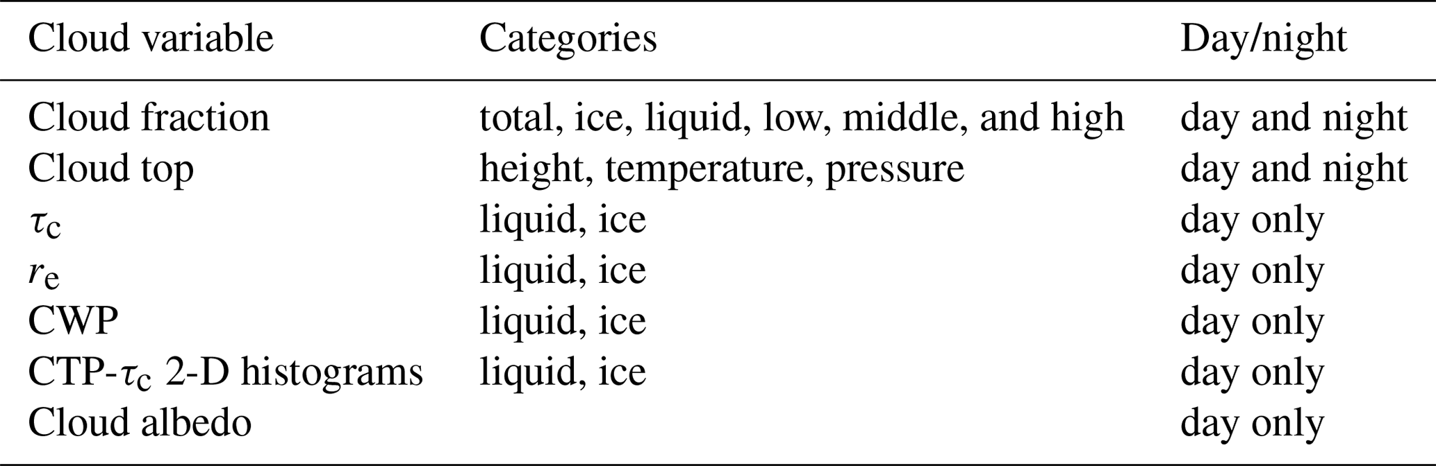
Table 1The cloud variables produced by the simulator. The middle column specifies the separate categories available for each variable, and the third column indicates under which illumination conditions the variables are available.
3.1 The impact of using a simulator on cloudiness
To demonstrate the importance of using satellite simulators for model-to-observation comparisons of cloud variables, we assess the separate impact of (1) sampling the model to match the satellite overpass times and (2) the impact of taking into account the underrepresentations of very thin clouds in the dataset due to limited satellite sensor sensitivities. These two aspects influence the simulations to a different extent depending on the variable. First we demonstrate the consequence of diurnal sampling on LWP, one of the variables expected to be strongly impacted by the diurnal cycle.
3.1.1 Temporal sampling
To not take the temporal sampling of the satellites into account is a potentially strong error source in model-to-satellite comparisons for certain cloud variables such as cloud water, with the uncertainty increasing with increasing model resolution (Guan et al., 2013). So far, it is the responsibility of the user to ensure that the temporal sampling of the model matches that of the satellite, and many publications, such as Ban-Weiss et al. (2014), rightly take the equatorial overpass time (EOT) into account when doing model comparisons. However, if a user compares simulated output from the model directly to observations without taking into account the EOT of the satellites used to make the CDR, bias due to temporal sampling will be introduced. Figure 1 shows the EOT of the satellites used to make the AVHRR-PM version of the Cloud_cci CDR.
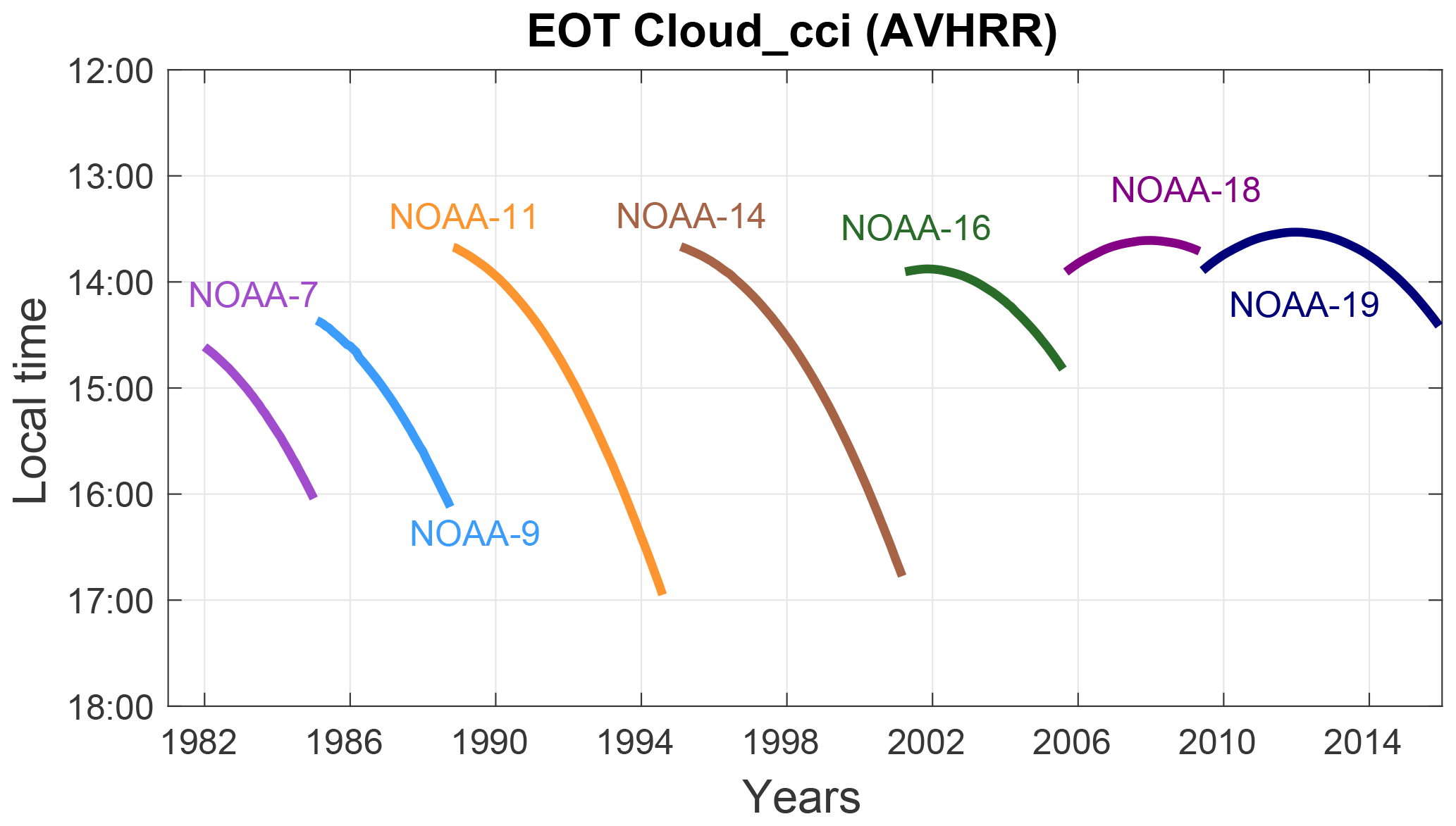
Figure 1The local time of EOT of the daytime (ascending) nodes of the satellites used to create the Cloud_cci AVHRR-PM CDR. The figure is a modified version of the same data in Stengel et al. (2017).
These polar-orbiting satellites start sampling the Earth during mid-afternoon1 globally at the start of their lifetime, but the local time of sampling “drifts” slowly over time if a satellite does not actively compensate for this. For instance, at the start of the period when the Cloud_cci CDR is based on NOAA-11 (November 1988), the EOT is around 13:30 LT, and just before switching data source to NOAA-14 (February 1995), the EOT is close to 17:00 LT. Especially in areas where the diurnal cycle of clouds or their properties is strong, the effect of sampling the atmosphere at later and later local times may be misinterpreted as a cloud trend.
The impact of not taking the satellite overpass into account is demonstrated in Fig. 2 using the original model data (i.e., not simulations of Cloud_cci) of LWP, one of the variables impacted the hardest by temporal sampling (Guan et al., 2013). The average LWP is on the left, and the fractional deviation between the average LWP at 14:00 LT and the total-day average is on the right. 14:00 LT is the local time chosen for comparison here since it is near the nominal EOT of the ascending node of the afternoon satellites using this version of the Cloud_cci CDR (see Fig. 1).
As can be seen in Fig. 2, the largest biases can be between 50 % to 100 % when comparing the average at 14:00 LT to the average from all the model data. The biases at this local time are largely positive over land and negative (and smaller) over ocean at this sampling time. The bias is most prominent over tropical land, which tends to be more cloud-free in the morning, while very often thunderstorms develop in the afternoon, and in the oceanic regions off the west coasts of the continents where conditions are dominated by stratocumulus in the morning which mostly clear up during the day.
As can be seen in Fig. 1, there are periods in the CDR where the sampling EOT is far off 14:00 LT. For instance, for the periods near the end of NOAA-7 and NOAA-9, and longer periods near the end of the NOAA-11 and NOAA-14 data series, the EOT is 16:00 LT or later. At 17:00 LT, the extreme, the bias pattern is quite different with large areas of negative and positive differences compared to the day mean (not shown).
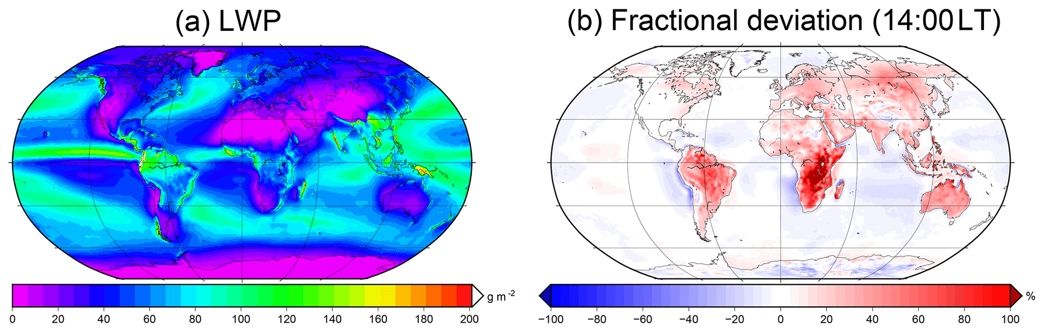
Figure 2The total average LWP from EC-Earth based on available all time steps (a), and the fractional deviation of the average LWP from sampling at 14:00 LT compared to the day average . The data are directly from the model from the period 1982 to 2014.
In general, the geographic regions where there is a strong diurnal cycle are expected to be where the largest sampling errors will occur. We decided, for the sake of reducing the temporal sampling bias, the Cloud_cci simulator should include the satellite overpass times as a function of year, month, and satellite so that the model can be automatically sampled at the local time that best matches the satellite and time period.
3.1.2 Cloud sensitivity
Using the basic cloud variable total cloud fraction (TCF), we demonstrate the combined effect of temporal sampling and removing clouds which are too thin to be retrieved in the Cloud_cci CDR. Figure 3 shows separately these two important effects of the simulator. The leftmost columns show the difference between sampling the data at the correct satellite overpass time and not sampling in this way. The center column shows the added benefit of removing the modeled clouds too thin to be detected by Cloud_cci compared to just sampling the model data correctly. The rightmost column shows the combined effect of temporal sampling and simulating the cloud sensitivity of Cloud_cci, i.e., the simulated Cloud_cci TCF, minus the TCF directly from the model. This column shows the total impact of the simulator on TCF.

Figure 3The simulated TCF minus the direct model output of TCF. Panels (a) and (d) show the impact of sampling the model to match the EOT of the satellites in a similar way as in Fig. 2 but this time for TCF and using the EOT shown in Fig. 1. It is the temporally sampled direct model output minus the direct model output (sampled–unsampled). Panels (b) and (e) show the simulated lack of sensitivity of the AVHRR sensor to optically very thin clouds (τc<0.2). Specifically, they show the simulated Cloud_cci minus the temporally sampled direct model output (simulated–sampled). Panels (c) and (f) show the combined impact on these two effects, i.e., clouds removed and temporal sampling, compared to the direct model output (simulated–unsampled). The top row is valid for DJF, and the bottom is for JJA. The data cover the period 1982–2014.
Overall, the simulator clearly reduces the TCF. The left column of Fig. 3 showing the difference between sampled and unsampled model data, illustrates that the effect of temporal sampling is important but nonetheless not as important as the effect of removing all thin clouds (center column) to the total difference between the simulated Cloud_cci and the unsampled model. This can be seen as most of the difference between the simulated TCF and the TCF straight from the model can be seen in the center column.
There are two important features to mention about the sampled–unsampled difference. Unlike LWP, TCF is retrieved both during daytime and nighttime, and therefore TCF is the average from two satellite overpasses per day, mostly around 14:00 and 02:00 LT (see Fig. 1), as opposed to LWP retrievals, which can only be retrieved during daylight hours (14:00 LT). Therefore, the error introduced by not sampling the model data is lower for day-and-night variables such as TCF compared to daylight-only variables.
Another feature is a clear interference pattern that is seen in the difference between the sampled and the unsampled model data. The longitudinal interference pattern appears at 90∘ intervals where the difference between the sampled and unsampled data reduces to exactly 0. This is a side effect from linearly interpolating between model time steps in order to sample the model data at a common local time that matches the EOT of the satellite. At evenly spaced longitudes, sampling the model to the ascending and descending EOTs is found from, for example, data at exactly 0.5×06:00 UTC + 0.5×12:00 UTC for the ascending node and 0.5×18:00 UTC + 0.5×24:00 UTC for the descending node. The average of these two interpolated values here is exactly the same as the average of the four model time steps at this longitude. This leads to a pattern of minimum and maximum differences that is repeated times, where N is the number of model time steps per day. The longitudes at which the minima are found depend on the EOT of the satellite. The interference patterns are a little blurred since the EOT is not constant over 33 years. This effect should also be present on top of any “real” differences whenever observational data based on two satellite overpasses per day are compared to model data when no attempt at temporal sampling has been made.
The global mean TCF is reduced by the simulator by about 10 %. As a reference, using CALIOP v4.0 data, we established that a global average of about 14 % are “thin clouds” (τc<0.2). Noteworthy from Fig. 3, the TCF is reduced by up to 20 % in some regions such as in large swaths of the tropics and polar regions, whereas for others such as at midlatitudes TCF is only lightly impacted. This can be explained by the model correctly reflecting the observed high frequency of thin cirrus clouds in the tropical regions (Sassen et al., 2008) which are reclassified as cloud-free by the simulator. In the polar regions, EC-Earth tends to have a high frequency of very thin, and likely false, clouds which are also removed by the simulator. The regional distribution of the effect of the simulator on TCF is quite different depending on the season. The impact on TCF by the simulator over southeast Africa in JJA is an increase in cloudiness because the temporal sampling effect described in Sect. 3.1.1 has a positive sign and is larger than the reduction by removing thin clouds.
4.1 Cloud fraction
Several studies have made use of the layered cloud cover for assessing the climate variability in GCMs (Zhang et al., 2005). The cloud cover varies quite substantially on a seasonal basis as seen by comparing JJA, Fig. 4, and DJF, Fig. 5. The TCF is included in each figure for reference and is the sum of the low, middle, and high layers.
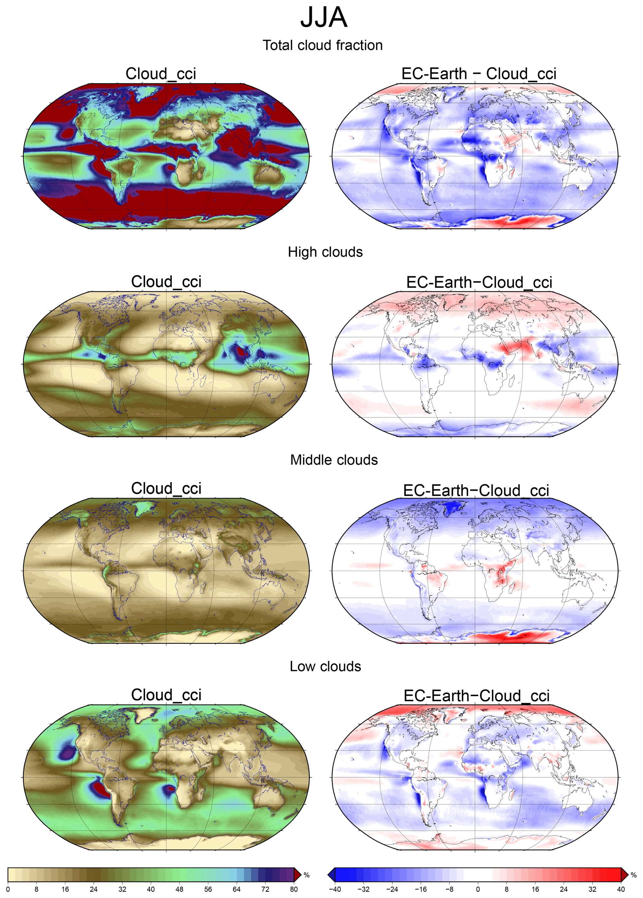
Figure 4Cloud fractions separated by cloud altitude from the Cloud_cci CDR (left column) and difference between the simulated Cloud_cci-based EC-Earth atmosphere and the observations (right column), separated into TCF (top row), high clouds (second row), mid-level clouds (third row), and low clouds (bottom row), for JJA.
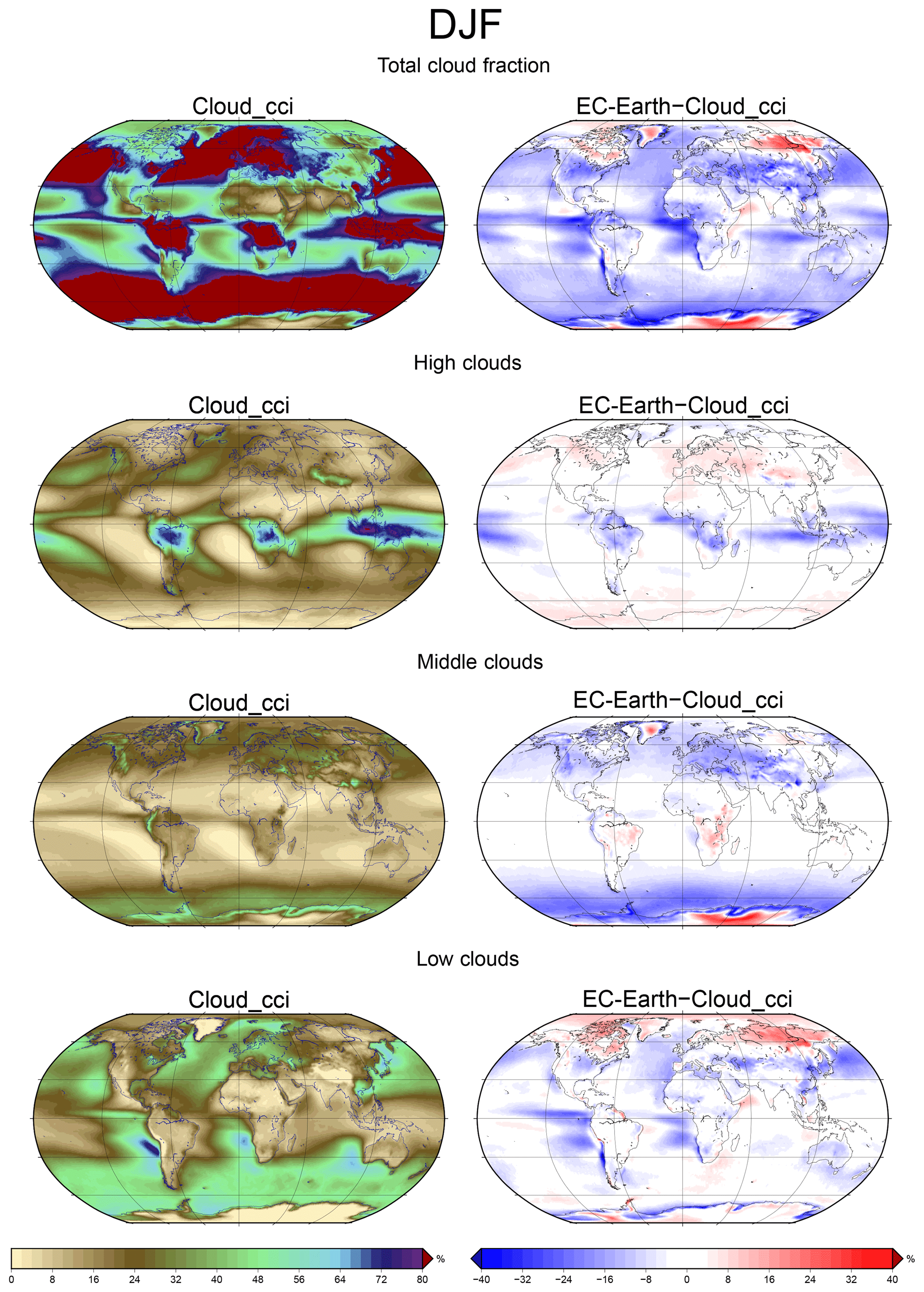
Overall, the distribution of high clouds is reasonably well captured by EC-Earth, although the simulations show an overall underestimation of tropical high cloud fraction. EC-Earth seems to have too few clouds associated with the Intertropical Convergence Zone in general in both seasons. Also, it appears that high clouds associated with the Indian monsoon may be too far west in EC-Earth during JJA as seen by the very large overrepresentation of high clouds over the Arabian subcontinent and sea (around 20 % more than the observations). There is a larger deficit of high clouds over tropical Africa and South America in JJA compared to DJF.
For low clouds, a prominent feature is the large deficit in (or large underprediction of) cloudiness in the subtropical maritime stratocumulus regions off the west coast of southern Africa, South America, and southern North America especially in JJA but also in DJF. EC-Earth's underestimation of low clouds in the subtropical stratocumulus regions relative to ISCCP observations was also noted by Lacagnina and Selten (2014). The underestimation of subtropical maritime clouds is common in climate models and is largely due to a lack of regional variability in low cloud fraction in these regions (Noda and Satoh, 2014), which is linked to the variability of atmospheric stability of the lower atmosphere (Sun et al., 2011).
Low clouds are also underpredicted in the storm track regions and midlatitude oceans compared to Cloud_cci in respective winter hemispheres, as was also found in the EC-Earth to ISCCP comparison study (Lacagnina and Selten, 2014). For the polar regions, low clouds are overestimated compared to Cloud_cci as previously found in Koenigk et al. (2013). However, the size of the deficit seen here may also be related to the temporal sampling of the model by the simulator. The left columns in Fig. 3 indicate that the largest reductions in cloudiness when comparing non-sampled to sampled model TCF are in the subtropical marine stratocumulus regions. This may indicate that on top of the general deficit in low clouds, a mismatch in the diurnal cycle between the model and observations may also play a role.
Outside the tropics, the model cloudiness may be quite reasonable if one takes into account that the Cloud_cci CDR may place some thin high clouds too low in altitude, artificially decreasing the high cloud fraction and increasing the amount of mid-level clouds. However, the strong negative cloud fraction bias in some regions can only be partially explained by this. The negative bias in tropical high clouds could be in part a consequence of the simulator removing too many clouds in these regions, or that the model has them optically too thin. But also, since this simulator, like the MODIS and ISCCP simulators, uses a global constant τc threshold, it may be a little too high for the tropics, and too low for other regions compared to the actual performance of the Cloud_cci cloud mask of this version of the dataset.
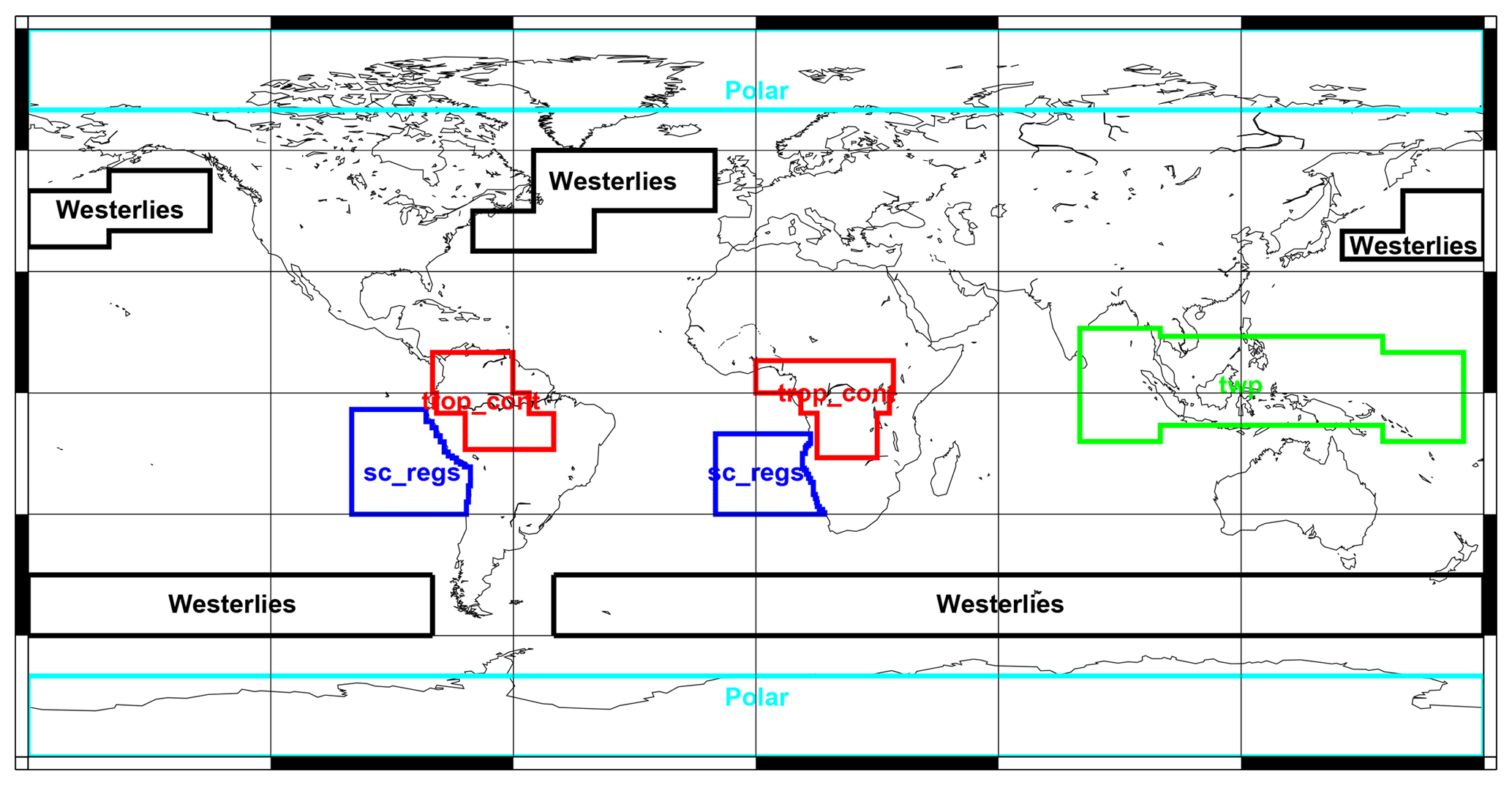
Figure 6A map of the regions selected for further investigation adapted from Eliasson et al. (2011, Fig. 9).
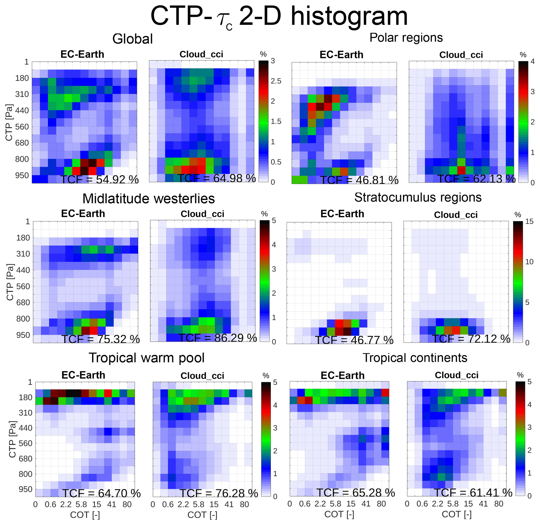
Figure 7CTP–τc histograms of simulated Cloud_cci based on EC-Earth (left column) and the Cloud_cci CDR (right column) for selected regions (see Fig. 6). Total cloud fractions for each region are indicated in the panels.
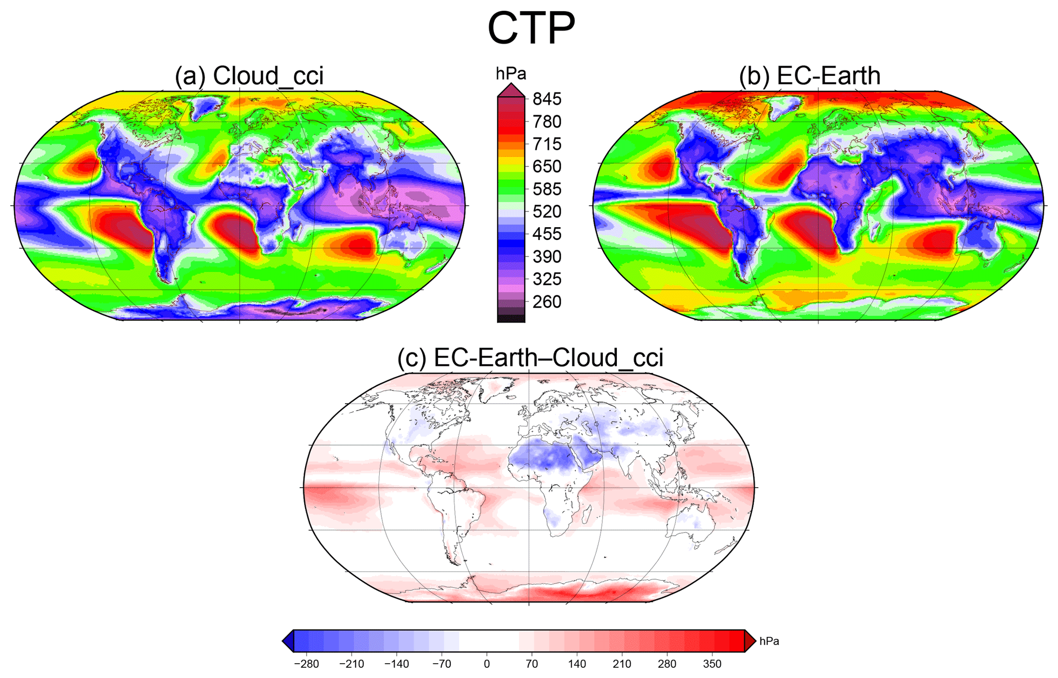
Figure 8The CTP from the Cloud_cci CDR (a), simulated CTP based on EC-Earth (b) and the difference between the two (c). The data cover the time period 1982–2014.
4.2 Cloud vertical distribution
By using the CTP-τc histograms shown in Fig. 7, more information on the difference in cloud vertical distribution can be found. Globally, EC-Earth is less cloudy than the Cloud_cci CDR by about 8 %. The CTP-τc distribution of clouds is quite different between the model and observations and better understanding of the differences can be found if one separates the distributions into separate climatological regions (Eliasson et al., 2011). Here, we focus on five non-contiguous regions shown on the map in Fig. 6.
In the polar regions, the vertical distribution of clouds deviates strongly from the Cloud_cci CDR. EC-Earth has a high frequency of relatively thin, middle–high clouds, a feature completely missing from the Cloud_cci CDR. However, the datasets' skill in the Arctic may be insufficient to make definitive claims about biases in the model. In the westerlies region, there are fewer mid-level clouds in the model than in the observations in general. This difference may be attributed to misclassifications of multi-layer clouds into mid-layer clouds by the Cloud_cci CDR, by the process mentioned in the previous section. The reason EC-Earth has a higher occurrence of high clouds in the westerlies region may be the same, but there are indications that EC-Earth has too many very optically thick high clouds in the westerlies regions.
In the maritime stratocumulus regions, the model clearly underestimates the amount of clouds by about 15 %, also underestimating the diversity, in terms of thickness and vertical distribution, of low clouds compared to the Cloud_cci CDR. In the tropical warm pool region, EC-Earth is less cloudy but tends to have substantially thicker clouds. In the tropical continental regions, EC-Earth erroneously has many more mid-level, optically thick clouds and is missing the regular occurrence of low-level thin clouds. EC-Earth also has relatively much more high-level thin clouds compared to observations, although it has a lower total cloud fraction. Quite potentially, the mid-level clouds in the model are too thick.
Cloud top pressure
The mean CTP is shown in Fig. 8. Overall, the cloud top pressure in the midlatitude regions is fairly close to the observations. However, there are other areas with large differences such as the polar regions, where EC-Earth has much higher CTP (lower cloud top height), but the polar regions are also difficult places for cloud retrievals from any passive instrument, since very cold regions risk having a bias towards lower level clouds as high clouds have similar cloud and surface temperatures. This makes retrievals in these regions quite uncertain. More important are the differences found in the tropics since clouds there are generally easier to retrieve due to the large temperature contrast between the warm surface and especially mid- and high-level clouds. EC-Earth tends to overestimate the CTP compared to the Cloud_cci CDR around the outskirts of the tropical warm pool and especially in the central Pacific, a region where clouds are heavily influenced by the ENSO. In contrast, in a large region covering north Africa and the Arabian subcontinent, the clouds in the model appear much higher (lower CTP) compared to the Cloud_cci retrievals. This may be a consequence of too many high clouds, as mentioned in the previous section, or the effect of thin high cirrus over the desert (which has a lower surface emissivity) being retrieved as mid-level clouds, or a combination of these reasons.
4.3 Effective radius
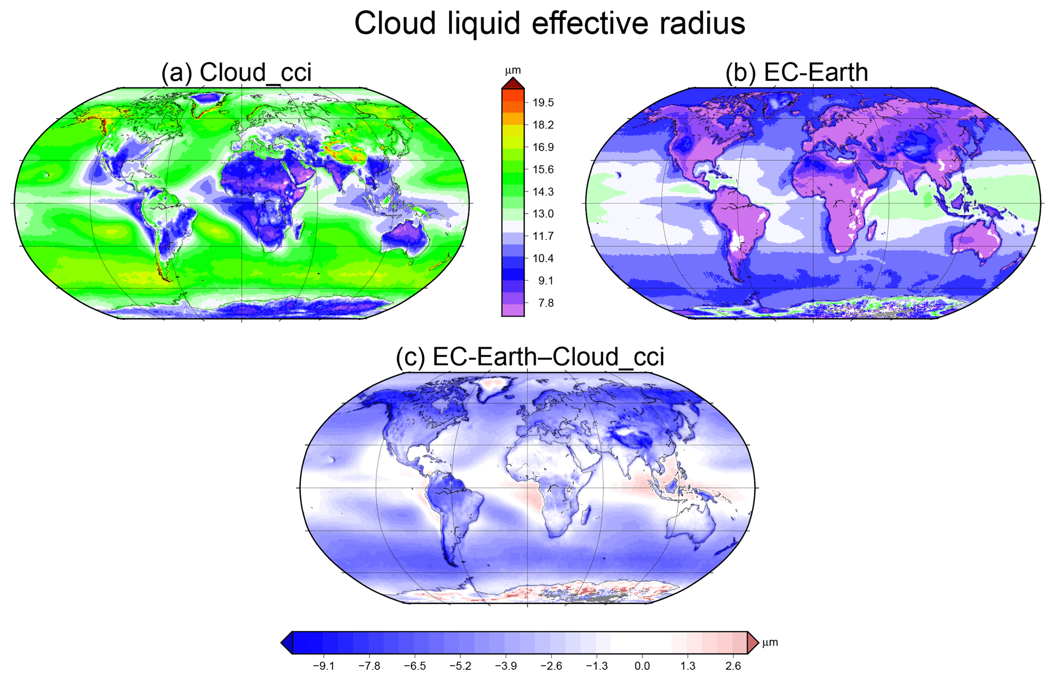
Cloud microphysical properties strongly influence the radiative budget and also the water cycle. However, properties such as re may be difficult to compare between models and satellite observations since their uncertainties are quite large and depend strongly on the assumptions, such as optical properties of cloud particles, that must be made in the retrieval process.
The differences between EC-Earth and the Cloud_cci CDR are substantial. As can be seen in Fig. 9, the differences are very large in terms of liquid cloud re. There is a very distinct land–sea difference, which is likely a reflection of the model re parameterizations based on Martin et al. (1994). These depend in part on the assumed aerosol concentrations, which are largely different over land and sea. EC-Earth assumes one constant concentration of 900 cm3 over land and 50 cm3 over sea. However, the differences can also be due to problems of the re retrievals, e.g., for broken and multi-layer clouds. There is also a strong disagreement in terms of ice re (not shown). The skill of the retrieved ice cloud re in the version of the Cloud_cci CDR presented here (v2.0) is questionable according to Stengel et al. (2017) and therefore left out in the comparisons for EC-Earth and RACMO in the next section. Overall, the observations and EC-Earth are in disagreement for re and deeper analysis is needed to find the sources to these differences.
This section describes the performance of the RCM, RACMO compared to the Cloud_cci CDR using the satellite simulator. In Fig. 10, time series of RACMO cloud property simulations are compared with the Cloud_cci CDR retrievals for two selected areas: in the Atlantic and in northwest Europe (see Fig. 11a for the location of these areas). For these regions, the simulator does not change the RACMO TCF much; i.e., the contribution of thin clouds is very small. Note that this differs somewhat from the EC-Earth run, which has, especially over the Atlantic region, a larger amount of thin clouds and consequently a stronger reduction in TCF induced by the simulator (see Fig. 3). Compared to the satellite observations, the model overestimates TCF in the Atlantic, while the opposite is true over northwest Europe.
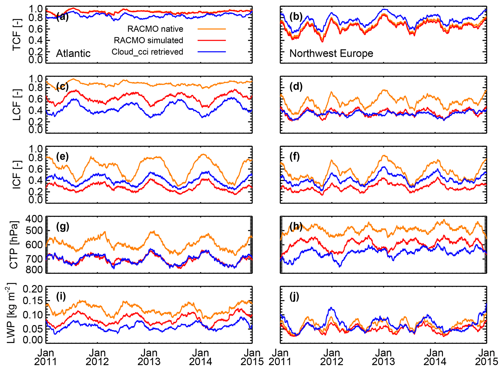
Figure 10Time series of RACMO native model (orange), simulated (red), and Cloud_cci retrieved (blue) cloud properties for areas in the Atlantic (left; 48–53∘ N, 25–15∘ W) and northwest Europe (right; 48–53∘ N, 5–15∘ E) during 2011–2014: (a, b) total cloud fraction, (c, d) liquid cloud fraction, (e, f) ice cloud fraction, (g, h) CTP (hPa), and (i, j) LWP (kg m−2). Shown are 2-month running means. All properties are all-sky linear averages, except CTP, which is an in-cloud logarithmic average.
The cloud fraction is further separated into liquid and ice cloud fractions (LCFs/ICFs). In the model, a grid box can contribute to both cloud fractions, so the sum of the LCF and ICF will in general be larger than TCF. In the simulator, as well as in the retrieval, a column is either designated the liquid or the ice phase, so that the two fractions will add up to TCF. As a result, the simulator decreases both LCF and ICF compared to the native model, making it much more comparable to the retrievals. The CTP in the model is much smaller than retrieved; i.e., the cloud tops are higher. The simulator increases log-mean CTP by about 100 hPa in both regions by removing modeled thin high cloud layers, bringing it much closer to the satellite retrieval. To multiphase clouds in the model (typically ice above liquid), the simulator will tend to designate the ice phase. The liquid water in the lower clouds is then basically interpreted as ice. Consequently, the simulated LWP is smaller than in the native model. In the Atlantic, this leads to a closer agreement with the satellite observations. In northwest Europe, the native model LWP is on average already comparable to the satellite measurements, and the simulator turns this into an underestimation.
For the Cloud_cci CDR and the areas shown in Fig. 10, the correlation coefficient (Pearson's r) between simulated and retrieved time series ranges between 0.55 (for TCF over the Atlantic) and 0.86 (for TCF in northwest Europe and ICF in both regions). In general, the simulated time series correlate (much) better with the retrievals than the native model time series. As an indication, the mean correlation coefficients for the two regions and five parameters considered are 0.56 and 0.74 for the native modeled and simulated time series, respectively.
Spatial distributions of modeled and retrieved cloud properties are shown in Fig. 11. As noted before, the simulator has a relatively small impact on RACMO TCF, with a reduction of about 2 % over the model domain. The modeled and retrieved spatial patterns in TCF correspond rather well. Note, for example, the agreement in orography-related TCF patterns in the Alps and Carpathians. However, the model (and simulated) TCF is higher than the retrieval over the Atlantic, particularly in the southern part of the domain, where differences reach 20 %. The opposite is true over most of the continent, including the Baltic Sea and the Black Sea. An underestimation of RACMO TCF compared with satellite retrievals over the (western) European continent was also found by Roebeling and van Meijgaard (2009).

Figure 11Maps of 2011–2014 mean modeled and retrieved cloud properties: (a–d) total cloud fraction, (e–h) cloud top pressure (hPa), (i–l) LWP (kg m−2), (m–p) liquid τc, and (q–t) liquid re (µm). The columns show from left to right the native model, the simulator, the Cloud_cci data, and the difference between simulator and retrieval. All properties are all-sky averages, except CTP and re, which are in-cloud averages. In addition, CTP has been logarithmically averaged, while the other properties have been linearly averaged. Panel (a) shows the areas defined for the time series analysis in Fig. 10.
For CTP, the agreement between the simulated model results and the retrievals is rather good over the Atlantic, while over land the modeled clouds have higher tops (lower CTP) than retrieved, even after the simulator has been applied. LWP patterns of simulator–retrieval differences are rather similar to those for TCF. These patterns can be roughly understood from the generally higher TCF and τc in the simulated model results over ocean, and the lower TCF and re over land. The liquid re plots reflect the simple parameterization of re in the model, depending on fixed, and very different, aerosol concentrations over land and water (see Sect. 4.3). This results in a sharp land–sea gradient in the modeled/simulated re, with much smaller droplets over land. Since the τc for model layers is determined from liquid/ice water content and re, τc shows an opposite gradient with strongly enhanced τc values over land. Such features can be improved if actual aerosol data are introduced for the calculation of re. Apart from this land–sea artifact in τc related to re, the model also appears to overestimate LWP and liquid τc in particular near the western coasts of the continent.
A Cloud_cci satellite simulator has been developed to test the performance of model clouds compared to the new satellite CDR, Cloud_cci. In this study, we have assessed certain aspects of cloudiness in the EC-Earth GCM and the RACMO RCM.
Firstly, the impact of using the simulator compared to just relying on the “native” model is shown using the TCF. In large areas, more than 20 % of the cloud cover is reduced by the simulator through the process of removing thin clouds, although the average global reduction is around 10 %. This is in line with the reality that the Cloud_cci retrievals tend to not detect clouds that are optically thinner than a global average of around τc=0.2. We also demonstrated the importance of sampling the model at the correct local time to match the EOT of the satellites used in the Cloud_cci CDR. As was illustrated with model LWP, large areas may have up to 50 % too much or too little LWP only due to sampling errors if the satellite overpass time has drifted by 4 h or so, and this mainly impacts the areas with a large diurnal cycle. For this reason, the simulator automatically samples the model at the EOT of the satellites used in the Cloud_cci CDR.
Overall, EC-Earth produces much the same cloudiness as seen in observations, with some key differences. For instance, in the tropics, the cloud tops are too low in the model, especially in the central Pacific region, whereas over north Africa and the Arabian subcontinent the clouds in EC-Earth appear too high. However, the desert areas tend to be dominated by thin high clouds, a cloud type that tends to be biased low for Cloud_cci (Stengel et al., 2017). There are also very large differences between EC-Earth and Cloud_cci in terms of re.
The evaluation of RACMO indicates some biases with respect to the Cloud_cci data. In particular, cloud amount is higher in the model over the northern Atlantic. In contrast, over continental Europe, the modeled cloud amount is lower, and the modeled CTP is – even after a considerable enhancement implied by the simulator – lower than retrieved.
Overall, the results shown here convincingly demonstrate that a simulator is needed to make meaningful comparisons between modeled and retrieved cloud properties. It is promising to see that for (nearly) all cloud properties the simulator improves the agreement of the model with the satellite data.
Cloud_cci CDR (Stengel et al., 2017) can be downloaded from http://www.esa-cloud-cci.org/?q=data_download (last access: 12 February 2019). Data from the EC-Earth global climate model (Hazeleger et al., 2010) can be obtained from http://www.nextdataproject.it/?q=en/content/ec-earth-cmip5-data-extraction (last access: 12 February 2019), and data from the regional climate model RACMO (van Meijgaard et al., 2012) can be obtained through https://www.projects.science.uu.nl/iceclimate/models/racmo.php (last access: 12 February 2019).
The simulator code itself (https://doi.org/10.5281/zenodo.2533858; Eliasson, 2019) can be found at https://github.com/SatelliteSimulators/cloud_cci (last access: 12 February 2019).
SE is the main author. He wrote most of the article, carried out all the simulations of Cloud_cci from EC-Earth data, and made comparisons to the Cloud_cci CDR. JFM and EvM used the simulator on the RACMO model and co-wrote all the sections related to RACMO and their comparison to the observations. UW, who is a model developer for EC-Earth, provided valuable input from the climate modeler's perspective. MS and KGK provided the Cloud_cci CDR and provided valuable input from this CDR's perspective. All co-authors provided valuable editing help in each iteration of the article.
The authors declare that they have no conflict of interest.
This work was supported by the European Space Agency through the Cloud_cci
project (contract no. 4000109870/13/INB) and by the Swedish National Space
Board (grant agreement no./award no. 121/14).
Edited by: Klaus Gierens
Reviewed by: Dustin Swales and one
anonymous referee
Balsamo, G., Beljaars, A., Scipal, K., Viterbo, P., van den Hurk, B., Hirschi, M., and Betts, A. K.: A Revised Hydrology for the ECMWF Model: Verification from Field Site to Terrestrial Water Storage and Impact in the Integrated Forecast System, J. Hydrometeorol., 10, 623–643, https://doi.org/10.1175/2008JHM1068.1, 2009. a
Ban-Weiss, G. A., Jin, L., Bauer, S. E., Bennartz, R., Liu, X., Zhang, K., Ming, Y., Guo, H., and Jiang, J. H.: Evaluating clouds, aerosols, and their interactions in three global climate models using satellite simulators and observations, J. Geophys. Res., 119, 10876–10901, https://doi.org/10.1002/2014JD021722, 2014. a
Baró, R., Jiménez-Guerrero, P., Stengel, M., Brunner, D., Curci, G., Forkel, R., Neal, L., Palacios-Peña, L., Savage, N., Schaap, M., Tuccella, P., Denier van der Gon, H., and Galmarini, S.: Evaluating cloud properties in an ensemble of regional online coupled models against satellite observations, Atmos. Chem. Phys., 18, 15183–15199, https://doi.org/10.5194/acp-18-15183-2018, 2018. a
Bechtold, P., Semane, N., Lopez, P., Chaboureau, J.-P., Beljaars, A., and Bormann, N.: Representing Equilibrium and Nonequilibrium Convection in Large-Scale Models, J. Atmos. Sci., 71, 734–753, https://doi.org/10.1175/JAS-D-13-0163.1, 2014. a
Bodas-Salcedo, A., Webb, M. J., Bony, S., Chepfer, H., Dufresne, J.-L., Klein, S. A., Zhang, Y., Marchand, R., Haynes, J. M., Pincus, R., and John, V. O.: COSP: satellite simulation software for model assessment, B. Am. Meteorol. Soc., 92, 1023–1043, https://doi.org/10.1175/2011BAMS2856.1, 2011. a
Boussetta, S., Simarro, C., and Lucas, D.: Exploring EC-Earth 3.2-Beta performance on the new ECMWF Cray-Broadwell, available at: https://www.ecmwf.int/en/elibrary/16377-exploring-ec-earth-32-beta-performance-new-ecmwf-cray-broadwell (last access: 12 February 2019), 2016. a
Bugliaro, L., Zinner, T., Keil, C., Mayer, B., Hollmann, R., Reuter, M., and Thomas, W.: Validation of cloud property retrievals with simulated satellite radiances: a case study for SEVIRI, Atmos. Chem. Phys., 11, 5603–5624, https://doi.org/10.5194/acp-11-5603-2011, 2011. a
Chepfer, H., Bony, S., Winker, D., Chiriaco, M., Dufresne, J.-L., and Sèze, G.: Use of CALIPSO lidar observations to evaluate the cloudiness simulated by a climate model, Geophys. Res. Lett., 35, L15704, https://doi.org/10.1029/2008GL034207, 2008. a
Clough, S. A., Shephard, M. W., Mlawer, E. J., Delamere, J. S., Iacono, M., Cady-Pereira, K., Boukabara, S., and Brown, P. D.: Atmospheric radiative transfer modeling: a summary of the AER codes, J. Quant. Spectrosc. Ra., 91, 233–244, https://doi.org/10.1016/j.jqsrt.2004.05.058, 2005. a
Eliasson, S.: SatelliteSimulators/cloud_cci: Cloud_cci satellite product simulator, Zenodo, https://doi.org/10.5281/zenodo.2533858, 2019. a
Eliasson, S., Buehler, S. A., Milz, M., Eriksson, P., and John, V. O.: Assessing observed and modelled spatial distributions of ice water path using satellite data, Atmos. Chem. Phys., 11, 375–391, https://doi.org/10.5194/acp-11-375-2011, 2011. a, b
Giorgi, F. and Gutowski, W. J.: Regional Dynamical Downscaling and the CORDEX Initiative, Annu. Rev. Environ., 40, 467–490, https://doi.org/10.1146/annurev-environ-102014-021217, 2015. a
Guan, B., Waliser, D. E., Li, J.-L. F., and da Silva, A.: Evaluating the impact of orbital sampling on satellite-climate model comparisons, J. Geophys. Res., 118, 1–15, https://doi.org/10.1029/2012JD018590, 2013. a, b
Haynes, J. M., Marchand, R. T., Luo, Z., Bodas-Salcedo, A., and Stephens, G. L.: A Multipurpose Radar Simulation Package: QuickBeam, B. Am. Meteorol. Soc., 88, 1723–1727, https://doi.org/10.1175/BAMS-88-11-1723, 2007. a
Hazeleger, W., Severijns, C., Semmler, T., Ştefănescu, S., Yang, S., Wang, X., Wyser, K., Dutra, E., Baldasano, J. M., Bintanja, R., Bougeault, P., Caballero, R., Ekman, A. M. L., Christensen, J. H., van den Hurk, B., Jimenez, P., Jones, C., Kållberg, P., Koenigk, T., McGrath, R., Miranda, P., van Noije, T., Palmer, T., Parodi, J. A., Schmith, T., Selten, F., Storelvmo, T., Sterl, A., Tapamo, H., Vancoppenolle, M., Viterbo, P., and Willén, U.: EC-Earth: A Seamless Earth System Prediction Approach in Action, B. Am. Meteorol. Soc., 91, 1357–1364, https://doi.org/10.1175/2010BAMS2877.1, 2010. a, b
Heidinger, A. K., Foster, M. J., Walther, A., and Zhao, X.: The Pathfinder Atmospheres–Extended AVHRR Climate Dataset, B. Am. Meteorol. Soc., 95, 909–922, https://doi.org/10.1175/BAMS-D-12-00246.1, 2014. a
IPCC: Clouds and Aerosols, in: Climate change 2013 – The physical science basis: Working Group I contribution to the fifth assessment report of the Intergovernmental Panel on Climate Change, 571–658, Cambridge University Press, Cambridge, https://doi.org/10.1017/CBO9781107415324.016, 2014. a
Jakob, C. and Klein, S. A.: The role of vertically varying cloud fraction in the parametrization of microphysical processes in the ECMWF model, Q. J. Roy. Meteor. Soc., 125, 941–965, https://doi.org/10.1002/qj.49712555510, 1999. a, b
Jonkheid, B. J., Roebeling, R. A., and van Meijgaard, E.: A fast SEVIRI simulator for quantifying retrieval uncertainties in the CM SAF cloud physical property algorithm, Atmos. Chem. Phys., 12, 10957–10969, https://doi.org/10.5194/acp-12-10957-2012, 2012. a
Karlsson, K.-G. and Devasthale, A.: Inter-comparison and Evaluation of the Four Longest Satellite-Derived Climate Data Records: CLARA-A2, ESA Cloud CCI V3, ISCCP-HGM and PATMOS-x, Remote Sensing, 10, 1567, https://doi.org/10.3390/rs10101567, 2018. a
Karlsson, K.-G. and Håkansson, N.: Characterization of AVHRR global cloud detection sensitivity based on CALIPSO-CALIOP cloud optical thickness information: demonstration of results based on the CM SAF CLARA-A2 climate data record, Atmos. Meas. Tech., 11, 633–649, https://doi.org/10.5194/amt-11-633-2018, 2018. a, b, c, d, e
Karlsson, K.-G., Anttila, K., Trentmann, J., Stengel, M., Fokke Meirink, J., Devasthale, A., Hanschmann, T., Kothe, S., Jääskeläinen, E., Sedlar, J., Benas, N., van Zadelhoff, G.-J., Schlundt, C., Stein, D., Finkensieper, S., Håkansson, N., and Hollmann, R.: CLARA-A2: the second edition of the CM SAF cloud and radiation data record from 34 years of global AVHRR data, Atmos. Chem. Phys., 17, 5809–5828, https://doi.org/10.5194/acp-17-5809-2017, 2017. a
Kay, J. E., Hillman, B. R., Klein, S. A., Zhang, Y., Medeiros, B., Pincus, R., Gettelman, A., Eaton, B., Boyle, J., Marchand, R., and Ackerman, T. P.: Exposing Global Cloud Biases in the Community Atmosphere Model (CAM) Using Satellite Observations and Their Corresponding Instrument Simulators, J. Climate, 25, 5190–5207, https://doi.org/10.1175/JCLI-D-11-00469.1, 2012. a
Keller, M., Kröner, N., Fuhrer, O., Lüthi, D., Schmidli, J., Stengel, M., Stöckli, R., and Schär, C.: The sensitivity of Alpine summer convection to surrogate climate change: an intercomparison between convection-parameterizing and convection-resolving models, Atmos. Chem. Phys., 18, 5253–5264, https://doi.org/10.5194/acp-18-5253-2018, 2018. a
Klein, S. A., Zhang, Y., Zelinka, M. D., Pincus, R., Boyle, J., and Gleckler, P. J.: Are climate model simulations of clouds improving? An evaluation using the ISCCP simulator, J. Geophys. Res., 118, 1–14, https://doi.org/10.1002/jgrd.50141, 2013. a
Koenigk, T., Brodeau, L., Graversen, R. G., Karlsson, J., Svensson, G., Tjernström, M., Willén, U., and Wyser, K.: Arctic climate change in 21st century CMIP5 simulations with EC-Earth, Clim. Dynam., 40, 2719–2743, https://doi.org/10.1007/s00382-012-1505-y, 2013. a
Lacagnina, C. and Selten, F.: Evaluation of clouds and radiative fluxes in the EC-Earth general circulation model, Clim. Dynam., 43, 2777–2796, https://doi.org/10.1007/s00382-014-2093-9, 2014. a, b
Lauer, A., Eyring, V., Righi, M., Buchwitz, M., Defourny, P., Evaldsson, M., Friedlingstein, P., de Jeu, R., de Leeuw, G., Loew, A., Merchant, C. J., Müller, B., Popp, T., Reuter, M., Sandven, S., Senftleben, D., Stengel, M., Roozendael, M. V., Wenzel, S., and Willén, U.: Benchmarking CMIP5 models with a subset of ESA CCI Phase 2 data using the ESMValTool, Remote Sens. Environ., 203, 9–39, https://doi.org/10.1016/j.rse.2017.01.007, 2017. a
Lenderink, G. and Holtslag, A. A. M.: An updated length-scale formulation for turbulent mixing in clear and cloudy boundary layers, Q. J. Roy. Meteor. Soc., 130, 3405–3427, https://doi.org/10.1256/qj.03.117, 2004. a
Lohmann, U. and Neubauer, D.: The importance of mixed-phase and ice clouds for climate sensitivity in the global aerosol–climate model ECHAM6-HAM2, Atmos. Chem. Phys., 18, 8807–8828, https://doi.org/10.5194/acp-18-8807-2018, 2018. a
Martin, G. M., Johnson, D. W., and Spice, A.: The measurement and parameterization of effective radius of droplets in warm stratocumulus clouds, J. Atmos. Sci., 51, 1823–1842, https://doi.org/10.1175/1520-0469(1994)051<1823:TMAPOE>2.0.CO;2, 1994. a
McGarragh, G. R., Poulsen, C. A., Thomas, G. E., Povey, A. C., Sus, O., Stapelberg, S., Schlundt, C., Proud, S., Christensen, M. W., Stengel, M., Hollmann, R., and Grainger, R. G.: The Community Cloud retrieval for CLimate (CC4CL) – Part 2: The optimal estimation approach, Atmos. Meas. Tech., 11, 3397–3431, https://doi.org/10.5194/amt-11-3397-2018, 2018. a, b
Mlawer, E. J., Taubman, S. J., Brown, P. D., Iacono, M. J., and Clough, S. A.: Radiative transfer for inhomogeneous atmospheres: RRTM, a validated correlated-k model for the longwave, J. Geophys. Res., 102, 16663–16682, 1997. a
Morcrette, J.-J., Barker, H. W., Cole, J. N. S., Iacono, M. J., and Pincus, R.: Impact of a New Radiation Package, McRad, in the ECMWF Integrated Forecasting System, Mon. Weather Rev., 136, 4773–4798, https://doi.org/10.1175/2008MWR2363.1, 2008. a
Noda, A. T. and Satoh, M.: Intermodel variances of subtropical stratocumulus environments simulated in CMIP5 models, Geophys. Res. Lett., 41, 7754–7761, https://doi.org/10.1002/2014GL061812, 2014. a
Norris, J. R., Allen, R. J., Evan, A. T., Zelinka, M. D., O'Dell, C. W., and Klein, S. A.: Evidence for climate change in the satellite cloud record, Nature, 536, 72–75, https://doi.org/10.1038/nature18273, 2016. a, b
Pincus, R., Platnick, S., Ackerman, S. A., Hemler, R. S., and Hofmann, R. J. P.: Reconciling Simulated and Observed Views of Clouds: MODIS, ISCCP, and the Limits of Instrument Simulators, J. Climate, 25, 4699–4720, https://doi.org/10.1175/JCLI-D-11-00267.1, 2012. a, b, c
Rodgers, C. D.: Inverse methods for atmospheric sounding: theory and practice, Singapore, World Scientific, River Edge, N.J., 2009. a
Roebeling, R. A. and van Meijgaard, E.: Evaluation of the daylight cycle of model-predicted cloud amount and condensed water path over Europe with observations from MSG SEVIRI, J. Climate, 22, 1749–1766, https://doi.org/10.1175/2008JCLI2391.1, 2009. a
Sassen, K., Wang, Z., and Liu, D.: Global distribution of cirrus clouds from CloudSat/Cloud-Aerosol Lidar and Infrared Pathfinder Satellite Observations (CALIPSO) measurements, J. Geophys. Res., 113, 1–12, https://doi.org/10.1029/2008JD009972, 2008. a
Siebesma, A. P., Soares, P. M. M., and Teixeira, J.: A Combined Eddy-Diffusivity Mass-Flux Approach for the Convective Boundary Layer, J. Atmos. Sci., 64, 1230–1248, https://doi.org/10.1175/JAS3888.1, 2007. a
Song, H., Zhang, Z., Ma, P., Ghan, S., and Wang, M.: An Evaluation of Marine Boundary Layer Cloud Property Simulations in Community Atmosphere Model Using Satellite Observations: Conventional Sub-grid Parameterization vs. CLUBB, 31, 2299–2320, https://doi.org/10.1175/JCLI-D-17-0277.1, 2017. a
Stengel, M., Mieruch, S., Jerg, M., Karlsson, K.-G., Scheirer, R., Maddux, B., Meirink, J.-F., Poulsen, C., Siddans, R., Walther, A., and Hollmann, R.: The Clouds Climate Change Initiative: Assessment of state-of-the-art cloud property retrieval schemes applied to AVHRR heritage measurements, Remote Sens. Environ., 162, 363–379, https://doi.org/10.1016/j.rse.2013.10.035, 2015. a
Stengel, M., Stapelberg, S., Sus, O., Schlundt, C., Poulsen, C., Thomas, G., Christensen, M., Carbajal Henken, C., Preusker, R., Fischer, J., Devasthale, A., Willén, U., Karlsson, K.-G., McGarragh, G. R., Proud, S., Povey, A. C., Grainger, R. G., Meirink, J. F., Feofilov, A., Bennartz, R., Bojanowski, J. S., and Hollmann, R.: Cloud property datasets retrieved from AVHRR, MODIS, AATSR and MERIS in the framework of the Cloud_cci project, Earth Syst. Sci. Data, 9, 881–904, https://doi.org/10.5194/essd-9-881-2017, 2017. a, b, c, d, e, f
Stengel, M., Schlundt, C., Stapelberg, S., Sus, O., Eliasson, S., Willén, U., and Meirink, J. F.: Comparing ERA-Interim clouds with satellite observations using a simplified satellite simulator, Atmos. Chem. Phys., 18, 17601–17614, https://doi.org/10.5194/acp-18-17601-2018, 2018. a
Stephens, G. L.: Radiation Profiles in Extended Water Clouds. II: Parameterization Schemes, J. Atmos. Sci., 35, 2123–2132, 1978. a
Stephens, G. L., Vane, D. G., Boain, R. J., Mace, G. G., Sassen, K., Wang, Z., Illingworth, A. J., O'Connor, E. J., Rossow, W. B., Durden, S. L., Miller, S. D., Austin, R. T., Benedetti, A., Mitrescu, C., and the CloudSat Science Team: The CloudSat mission and the A-train, B. Am. Meteorol. Soc., 83, 1771–1790, 2002. a
Sun, F., Hall, A., and Qu, X.: On the relationship between low cloud variability and lower tropospheric stability in the Southeast Pacific, Atmos. Chem. Phys., 11, 9053–9065, https://doi.org/10.5194/acp-11-9053-2011, 2011. a
Sus, O., Stengel, M., Stapelberg, S., McGarragh, G., Poulsen, C., Povey, A. C., Schlundt, C., Thomas, G., Christensen, M., Proud, S., Jerg, M., Grainger, R., and Hollmann, R.: The Community Cloud retrieval for CLimate (CC4CL) – Part 1: A framework applied to multiple satellite imaging sensors, Atmos. Meas. Tech., 11, 3373–3396, https://doi.org/10.5194/amt-11-3373-2018, 2018. a
Swales, D. J., Pincus, R., and Bodas-Salcedo, A.: The Cloud Feedback Model Intercomparison Project Observational Simulator Package: Version 2, Geosci. Model Dev., 11, 77–81, https://doi.org/10.5194/gmd-11-77-2018, 2018. a
Tan, J., Oreopoulos, L., Jakob, C., and Jin, D.: Evaluating rainfall errors in global climate models through cloud regimes, Clim. Dynam., 50, 3301–3314, https://doi.org/10.1007/s00382-017-3806-7, 2017. a
Terai, C. R., Klein, S. A., and Zelinka, M. D.: Constraining the low-cloud optical depth feedback at middle and high latitudes using satellite observations, J. Geophys. Res., 121, 9696–9716, https://doi.org/10.1002/2016JD025233, 2016. a
Tiedtke, M.: A comprehensive mass flux scheme for cumulus parametrization in large-scale models, Mon. Weather Rev., 117, 1779–1800, 1989. a
Tiedtke, M.: Representation of clouds in large-scale models, Mon. Weather Rev., 121, 3040–3061, 1993. a
Tompkins, A. M., Gierens, K., and Rädel, G.: Ice supersaturation in the ECMWF integrated forecast system, Tech. rep., European Centre for Medium-Range Weather Forecasts ECMWF, Technical Memorandum, https://doi.org/10.1002/qj.14, 2007. a
Unden, P., Rontu, L., Järvinen, H., Lynch, P., Calvo, J., Cats, G., Cuxart, J., Eerola, K., Fortelius, C., Garcia-Moya, J. A., Jones, C., Geert, Lenderlink, G., Mcdonald, A., Mcgrath, R., Navascues, B., Nielsen, N. W., Degaard, V., Rodriguez, E., Rummukainen, M., Sattler, K., Sass, B. H., Savijarvi, H., Schreur, B. W., Sigg, R., and The, H.: HIRLAM-5 Scientific Documentation, 2002. a
KNMI (van den Hurk, B., Siegmund, P., Klein Tank, A. (Eds.), Attema, J., Bakker, A., Beersma, J., Bessembinder, J., Boers, R., Brandsma, T., van den Brink, H., Drijfhout, S., Eskes, H., Haarsma, R., Hazeleger, W., Jilderda, R., Katsman, C., Lenderink, G., Loriaux, J., van Meijgaard, E., van Noije, T., van Oldenborgh, G. J., Selten, F., Siebesma, P., Sterl, A., de Vries, H., van Weele, M., de Winter, R., and van Zadelhoff, G.-J.): KNMI'14: Climate Change scenarios for the 21st Century – A Netherlands perspective, Scientific Report WR2014-01, KNMI, De Bilt, the Netherlands, available at: http://www.climatescenarios.nl/ (last access: 12 February 2019), 2014. a
van Meijgaard, E., van Ulft, L. H., Lenderink, G., de Roode, S., Wipfler, L., Boers, R., and Timmermans, R. M. A.: Refinement and application of a regional atmospheric model for climate scenario calculations of Western Europe, Tech. rep., KNMI, De Bilt, the Netherlands, available at: http://climexp.knmi.nl/publications/FinalReport_KvR-CS06.pdf (last access: 12 February 2019), 2012. a, b, c
Voors, R., Donovan, D., Acarreta, J., Eisinger, M., Franco, R., Lajas, D., Moyano, R., Pirondini, F., Ramos, J., and Wehr, T.: ECSIM: the simulator framework for EarthCARE, Proceedings of SPIE, Vol. 6744, https://doi.org/10.1117/12.737738, 2007. a
Waliser, D. E., Li, J.-L. F., Woods, C. P., Austin, R. T., Bacmeister, J., Chern, J., Genio, A. D., Jiang, J. H., Kuang, Z., Meng, H., Minnis, P., Platnick, S., Rossow, W. B., Stephens, G. L., Sun-Mack, S., Tao, W.-K., Tompkins, A. M., Vane, D. G., Walker, C., and Wu, D.: Cloud ice: A climate model challenge with signs and expectations of progress, J. Geophys. Res., 114, D00A21, https://doi.org/10.1029/2008JD010015, 2009. a
Webb, M., Senior, C., Bony, S., and Morcrette, J.-J.: Combining ERBE and ISCCP data to assess clouds in the Hadley Centre, ECMWF and LMD atmospheric climate models, Clim. Dynam., 17, 902–922, https://doi.org/10.1007/s003820100157, 2001. a
Webb, M. J., Andrews, T., Bodas-Salcedo, A., Bony, S., Bretherton, C. S., Chadwick, R., Chepfer, H., Douville, H., Good, P., Kay, J. E., Klein, S. A., Marchand, R., Medeiros, B., Siebesma, A. P., Skinner, C. B., Stevens, B., Tselioudis, G., Tsushima, Y., and Watanabe, M.: The Cloud Feedback Model Intercomparison Project (CFMIP) contribution to CMIP6, Geosci. Model Dev., 10, 359–384, https://doi.org/10.5194/gmd-10-359-2017, 2017. a
Winker, D. M., Vaughan, M. A., Omar, A., Hu, Y., Powell, K. A., Liu, Z., Hunt, W. H., and Young, S. A.: Overview of the CALIPSO Mission and CALIOP Data Processing Algorithms, J. Atmos. Ocean. Tech., 26, 2310–2323, https://doi.org/10.1175/2009JTECHA1281.1, 2009. a
Young, A. H., Knapp, K. R., Inamdar, A., Hankins, W., and Rossow, W. B.: The International Satellite Cloud Climatology Project H-Series climate data record product, Earth Syst. Sci. Data, 10, 583–593, https://doi.org/10.5194/essd-10-583-2018, 2018. a
Zelinka, M. D., Randall, D. A., Webb, M. J., and Klein, S. A.: Clearing clouds of uncertainty, Nature Climate Change, 7, 674–678, 2017. a, b
Zhang, M. H., Lin, W. Y., Klein, S. A., Bacmeister, J. T., Bony, S., Cederwall, R. T., Del Genio, A. D., Hack, J. J., Loeb, N. G., Lohmann, U., Minnis, P., Musat, I., Pincus, R., Stier, P., Suarez, M. J., Webb, M. J., Wu, J. B., Xie, S. C., Yao, M.-S., and Zhang, J. H.: Comparing clouds and their seasonal variations in 10 atmospheric general circulation models with satellite measurements, J. Geophys. Res., 110, D15S02, https://doi.org/10.1029/2004JD005021, 2005. a
This is as the satellite ascends from south to north; the descending EOT is shifted 12 h from the ascending node.