the Creative Commons Attribution 4.0 License.
the Creative Commons Attribution 4.0 License.
 | 24 Apr 2019
The Beijing Climate Center Climate System Model (BCC-CSM): the main progress from CMIP5 to CMIP6
Yixiong Lu
Yongjie Fang
Xiaoge Xin
Laurent Li
Weiping Li
Weihua Jie
Jie Zhang
Yiming Liu
Li Zhang
Fang Zhang
Yanwu Zhang
Fanghua Wu
Jianglong Li
Min Chu
Zaizhi Wang
Xueli Shi
Xiangwen Liu
Min Wei
Anning Huang
Yaocun Zhang
Xiaohong Liu
The main advancements of the Beijing Climate Center (BCC) climate system model from phase 5 of the Coupled Model Intercomparison Project (CMIP5) to phase 6 (CMIP6) are presented, in terms of physical parameterizations and model performance. BCC-CSM1.1 and BCC-CSM1.1m are the two models involved in CMIP5, whereas BCC-CSM2-MR, BCC-CSM2-HR, and BCC-ESM1.0 are the three models configured for CMIP6. Historical simulations from 1851 to 2014 from BCC-CSM2-MR (CMIP6) and from 1851 to 2005 from BCC-CSM1.1m (CMIP5) are used for models assessment. The evaluation matrices include the following: (a) the energy budget at top-of-atmosphere; (b) surface air temperature, precipitation, and atmospheric circulation for the global and East Asia regions; (c) the sea surface temperature (SST) in the tropical Pacific; (d) sea-ice extent and thickness and Atlantic Meridional Overturning Circulation (AMOC); and (e) climate variations at different timescales, such as the global warming trend in the 20th century, the stratospheric quasi-biennial oscillation (QBO), the Madden–Julian Oscillation (MJO), and the diurnal cycle of precipitation. Compared with BCC-CSM1.1m, BCC-CSM2-MR shows significant improvements in many aspects including the tropospheric air temperature and circulation at global and regional scales in East Asia and climate variability at different timescales, such as the QBO, the MJO, the diurnal cycle of precipitation, interannual variations of SST in the equatorial Pacific, and the long-term trend of surface air temperature.
- Article
(17659 KB) - Full-text XML
- BibTeX
- EndNote


Changes in global climate and environment are the main challenges that human societies are facing with respect to sustainable development. Climate and environmental changes are often the consequence of the combined effects of anthropogenic influences and complex interactions among the atmosphere, hydrosphere, lithosphere, cryosphere, and biosphere of the Earth system. To better understand the behaviors of Earth's climate, and to predict its future evolution, appropriate new concepts and relevant methodologies need to be proposed and developed. Climate system models are effective tools to simulate the interactions and feedbacks in an objective manner, and to explore their impacts on climate and climate change. The Coupled Model Intercomparison Project (CMIP), organized under the auspices of the World Climate Research Programme's (WCRP) Working Group on Coupled Modelling (WGCM), started 20 years ago as a comparison of a handful of early global coupled climate models (Meehl et al., 1997). More than 30 models participated in phase 5 of CMIP (CMIP5, Taylor et al., 2012) and created an unprecedented dynamic in the scientific community to generate climate information and make it available for scientific research. Many of these models were then extended into Earth system models by including the representation of biogeochemical cycles. The Beijing Climate Center (BCC) effectively contributed to CMIP5 by running most of the mandatory and optional simulations.
The first generation of the Beijing Climate Center ocean–atmosphere Coupled Model BCC-CM1.0 was developed from 1995 to 2004 (e.g., Ding et al., 2002). It was mainly used for seasonal climate prediction. Since 2005, BCC has initiated the development of a new fully coupled climate modeling platform (Wu et al., 2010, 2013, 2014). In 2012, two versions of the BCC model were released: BCC-CSM1.1, with a coarse horizontal resolution T42 (approximately 280 km), and BCC-CSM1.1m, with a medium horizontal resolution T106 (approximately 110 km). The BCC model (both versions) was a fully coupled model with ocean, land surface, atmosphere, and sea-ice components (Wu et al., 2008; Wu, 2012; Xin et al., 2013). Both versions were extensively used for CMIP5. At the end of 2017, the second generation of the BCC model was released to run different simulations proposed by phase 6 of CMIP (CMIP6, Eyring et al., 2016). The purpose of this paper is to document the main efforts and advancements achieved in BCC with respect to its climate model transition from CMIP5 to CMIP6. We show improvements in both the model resolution and its physics. A relevant description of the model transition and experimental design are shown in Sects. 2 and 3. A comparison of the model performance is presented in Sect. 4. Conclusions and discussion are summarized in Sect. 5. Information regarding the code and the data availability is shown in Sect. 6.
Table 1 shows a summary of the different BCC models or versions used for CMIP5 and CMIP6; all of them are fully coupled global climate models with four components, atmosphere, ocean, land surface and sea ice, interacting with each other. They are physically coupled through fluxes of momentum, energy, and water at their interfaces. The coupling was realized using the flux coupler version 5 developed by the National Center for Atmosphere Research (NCAR). BCC-CSM1.1 and BCC-CSM1.1m are our two models involved in CMIP5. They differ mainly with respect to their horizontal resolutions. As shown in Table 1, BCC-CSM2-MR, BCC-CSM2-HR, and BCC-ESM1.0 are the three models developed for CMIP6.
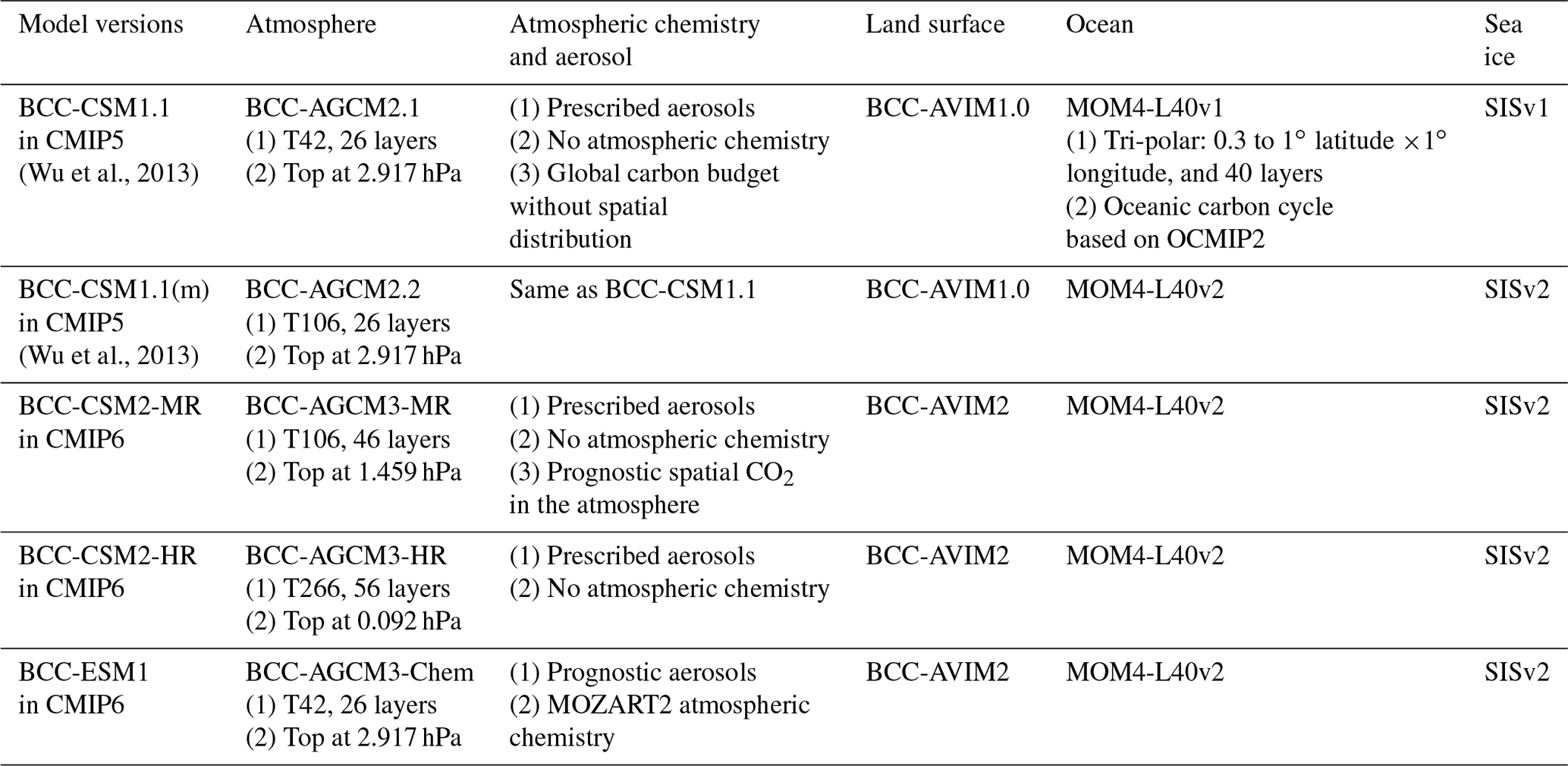
BCC-ESM1.0 is our Earth system configuration. It is a global fully coupled climate–chemistry–carbon model, and is intended to conduct simulations for the Aerosol Chemistry Model Intercomparison Project (AerChemMIP, Collins et al., 2017) and the Coupled Climate–Carbon Cycle Model Intercomparison Project (C4MIP, Jones et al., 2016), both endorsed by CMIP6. Its performance will be presented in a separated paper. BCC-CSM2-HR is our high-resolution configuration prepared for conducting simulations of the High Resolution Model Intercomparison Project (HighResMIP v1.0, Haarsma et al., 2016). It has 56 layers in the vertical and 0.092 hPa for the top of model. Its performance will also be presented separately.
In this paper, we focus on BCC-CSM1.1m and BCC-CSM2-MR. The two models are representative of our climate modeling efforts in CMIP5 and CMIP6, respectively. They have the same horizontal resolution (T106, about 110×110 km in the atmosphere, and 30×30 km in the tropical ocean), ensuring a fair comparison. But they have different vertical resolutions in the atmosphere (Table 1): 26 layers with its top at 2.917 hPa in BCC-CSM1.1m and 46 layers with its top at 1.459 hPa in BCC-CSM2-MR (Fig. 1). The present version of BCC-CSM2-MR requires 50 % more computing time than BCC-CSM1.1m for the same amount of parallel computing processors.
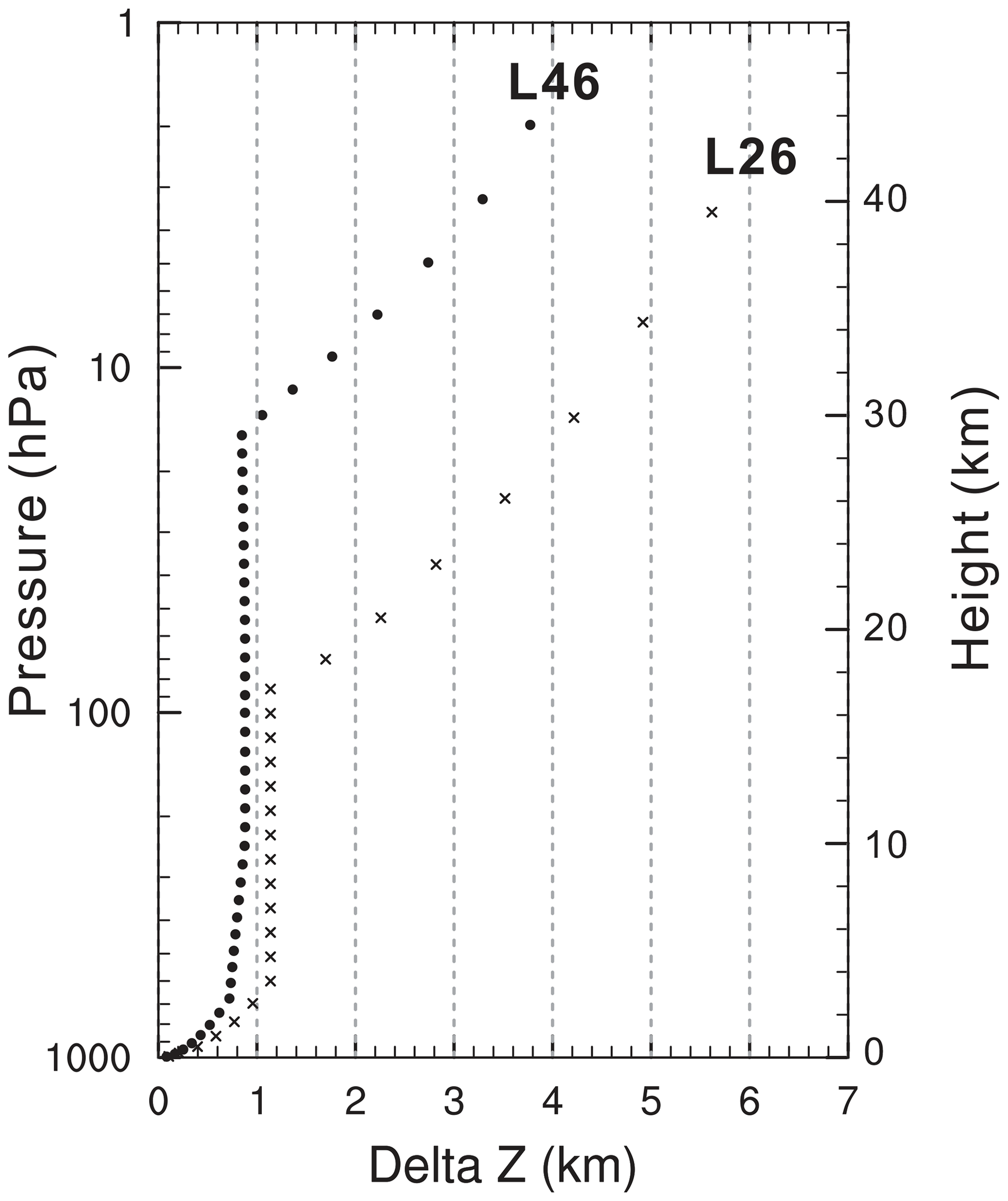
Figure 1The profiles of layer thickness against height for 26 vertical layers of the atmosphere in BCC-CSM-1.1m and 46 vertical layers in BCC-CSM2-MR.
2.1 Atmospheric component BCC-AGCM
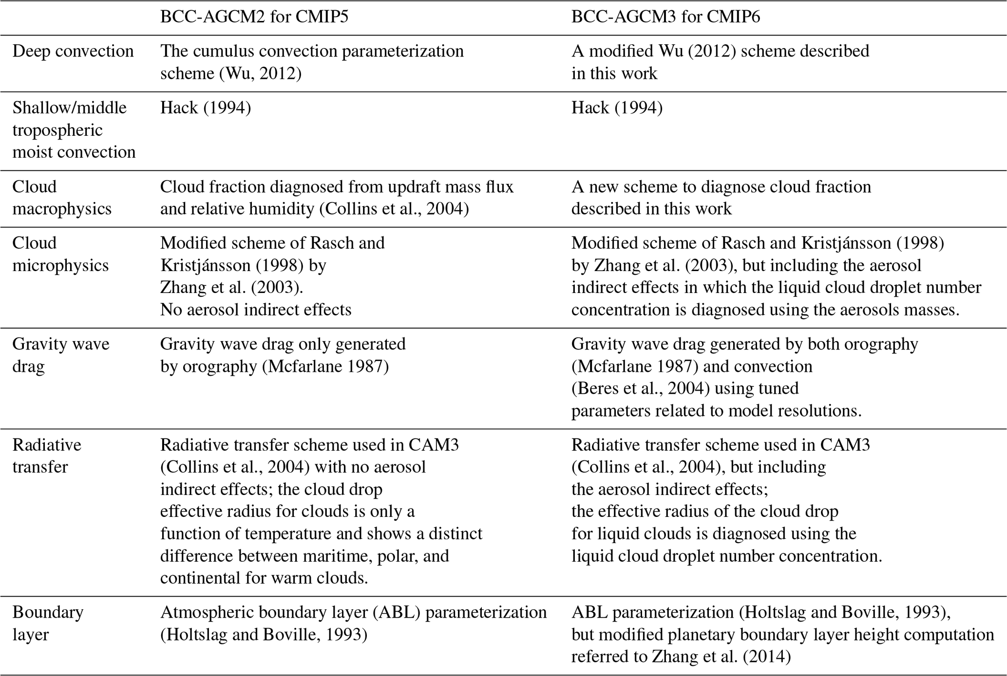
The atmospheric component of BCC-CSM1.1m is BCC-AGCM2.2 (second generation). It is detailed in a series of publications (Wu et al., 2008, 2010, 2013; Wu, 2012). BCC-AGCM3-MR is its updated version (third generation), used as the atmosphere component in BCC-CSM2-MR. The dynamic core in the two models is identical and uses the spectral framework described in Wu et al. (2008); within this framework a reference stratified atmospheric temperature and a reference surface pressure are introduced into the governing equations to improve pressure gradient force and gradients of surface pressure and temperature, and the prognostic variables for temperature and surface pressure are separately replaced by their perturbations from their references. An explicit time difference scheme is applied to the vorticity equation, and an semi-implicit time difference scheme is applied to the divergence, temperature, and surface pressure equations. A semi-Lagrangian tracer transport scheme is used for water vapor, liquid cloud water, and ice cloud water. The main differences in the model physics used in the two models (BCC-AGCM2.2 and BCC-AGCM3-MR) are summarized in Table 2 and detailed in the following.
Table 2Main physics schemes in the atmospheric components (BCC-AGCM) of the BCC-CSM versions for CMIP5 and CMIP6.
2.1.1 Deep convection
Our second-generation atmospheric model, BCC-AGCM2.2, operates with a parameterization scheme of deep cumulus convection developed by Wu (2012). The main characteristics can be summarized as follows:
-
Deep convection is initiated at the level of maximum moist static energy above the boundary layer. It is triggered when there is positive convective available potential energy (CAPE) and if the relative humidity of the air at the lifting level of convective cloud is greater than 75 %.
-
A bulk cloud model, taking the processes of entrainment/detrainment into account, is used to calculate the convective updraft with consideration of budgets for mass, dry static energy, moisture, cloud liquid water, and momentum. The scheme also considers the lateral entrainment of the environmental air into the unstable ascending parcel before it rises to the lifting condensation level. The entrainment/detrainment amount for the updraft cloud parcel is determined according to the increase/decrease of the updraft parcel mass with altitude. Based on a total energy conservation equation of the whole adiabatic system involving the updraft cloud parcel and the environment, the mass change for the adiabatic ascent of the cloud parcel with altitude is derived.
-
The convective downdraft is assumed to be saturated and to have originated from the level of minimum environmental saturated equivalent potential temperature within the updraft cloud.
-
The closure scheme determining the mass flux at the base of convective cloud is that suggested by Zhang (2002). It assumes that the increase/decrease of CAPE due to changes of the thermodynamic states in the free troposphere resulting from convection approximately balances the decrease/increase resulting from large-scale processes.
A modified version of Wu (2012) is used in BCC-AGCM3-MR for deep convection parameterization. The convection is only triggered when the boundary layer is unstable or when an updraft velocity in the environment exists at the lifting level of convective cloud, and there is simultaneously positive CAPE. This modification is aimed to connect the deep convection to the instability of the boundary layer. The lifting condensation level is set to above the nominal level of non-divergence (600 hPa) in BCC-AGCM2.2 and lowered to the level of 650 hPa in BCC-AGCM3-MR. These modifications in the deep convection scheme are found to improve the simulation of the diurnal cycle of precipitation and the Madden–Julian Oscillation (MJO).
2.1.2 Shallow convection
Shallow convection is parameterized with a local convective transport scheme (Hack, 1994). It is used to remove any local instability that may remain after the deep convection scheme. This Hack convection scheme is largely used to typically represent shallow subtropical convection and midlevel convection that do not originate from the boundary layer.
2.1.3 Cloud macrophysics
The cloud macrophysics comprises physical processes to compute cloud fractions in each layer, horizontal and vertical overlapping of clouds, and conversion rates of water vapor into cloud condensates. In BCC-AGCM2.2, the cloud fraction and the associated cloud macrophysics follow the NCAR Community Atmosphere Model version 3 (CAM3, Collins et al., 2004) design. The total cloud cover (Ctot) within each model grid is set as the maximum value of three cloud covers: low-level marine stratus (Cmst), convective cloud (Cconv), and stratus cloud (Cs):
As in CAM3, the marine stratocumulus cloud is diagnosed with an empirical relationship between the cloud fraction and the boundary layer stratification, which is evaluated with atmospheric variables at the surface and at 700 mb (Klein and Hartmann, 1993). The convective cloud fraction uses a functional form of Xu and Krueger (1991) relating the cloud cover to the updraft mass flux from the deep and shallow convection schemes. The stratus cloud fraction is diagnosed on the basis of relative humidity which varies with pressure.
A new cloud scheme is developed and used in BCC-AGCM3-MR. It consists of calculating convective cloud and the total cloud cover differently to BCC-AGCM2.2. The total cloud fraction in each model grid cell is given as
where the convective cloud (Cconv) is assumed to be the sum of shallow (Cshallow) and deep (Cdeep) convective cloud fractions:
Cshallow and Cdeep do not overlap with one another and are diagnosed using the following relationships:
and
where and , and denote the model grid box-averaged water vapor mixing ratio and temperature in the “environment” before and after convection activity, respectively. Tc and q* (Tc) are the respective temperature inside the convective cloud plume and its saturated water vapor mixing ratio. Here, we assume that shallow and deep convection can concurrently occur in the same atmospheric column at any time step. That is, the shallow convection scheme follows the deep convection and occurs at vertical layers where local instability still remains after deep convection.
If no supersaturation exists in clouds, we can obtain the following from Eqs. (4) and (5):
The temperature Tc and the specific humidity of the cloud plume can be firstly derived from Eqs. (5) and (6). Following the method above, the cloud fraction (Cdeep and Cshallow), temperature (Tdeep and Tshallow), and specific humidity (qdeep and qshallow) for the respective deep and shallow convective clouds can be then deduced sequentially.
After the three moisture processes (i.e., deep convection, shallow convection, and finally stratiform precipitation) are finished, the mean temperature () and specific humidity () of the whole model-grid box are then updated. Ambient temperature () and specific humidity () outside convective clouds can be finally estimated using the following equations:
and
Finally, the stratus cloud fraction CS is diagnosed on the basis of the ambient relative humidity (RHambient):
where RHmin is a threshold of relative humidity and RHambient is derived using and . If in Eqs. (8) and (9), Cdeep and Cshallow are scaled to meet the condition , then Cs=0. Under this condition, we do not calculate and from Eqs. (8) and (9).
2.1.4 Cloud microphysics
In BCC-AGCM2.2 and BCC-AGCM3-MR, the essential part of the stratiform cloud microphysics remains the same and follows the framework of non-convective cloud processes in CAM 3.0 (Collins et al., 2004), which is the scheme proposed by Rasch and Kristjánsson (1998) and modified by Zhang et al. (2003). However there is a noticeable difference in the cloud microphysics in the two models concerning the treatments for indirect effects of aerosols through mechanisms of clouds and precipitation. Indirect effects of aerosols were not included in BCC-AGCM2.2 for CMIP5. That is, the effective radius of cloud droplets was not related to aerosols or the precipitation efficiency. The cloud droplets effective radius was either prescribed or was a simple function of atmospheric temperature. The effective radius for warm clouds was specified as 14 µm over open ocean and sea ice, and was a function of atmospheric temperature over land. For ice clouds, the effective radius was also a function of temperature following Kristjánsson et al. (2000).
Aerosol particles influence clouds and the hydrological cycle by their ability to act as cloud condensation nuclei and ice nuclei. This indirect radiative forcing of aerosols is included in the latest version of BCC-AGCM3-MR, with the effective radius of liquid water cloud droplets being related to the cloud droplet number concentration Ncdnc (cm−3). As proposed by Martin et al. (1994), the volume-weighted mean cloud droplet radius rl, vol can be expressed as
where ρw is the liquid water density, and LWC is the cloud liquid water content (g cm−3). Cloud water and ice contents are prognostic variables in our model with source and sink terms taking the cloud microphysics into account. The effective radius of cloud droplets rel is then estimated as
where β is a parameter dependent on the droplets spectral shape. There are various methods to parameterize this variable (e.g., Pontikis and Hicks, 1992; Liu and Daum, 2002). We use the calculation proposed by Peng and Lohmann (2003):
In BCC-AGCM3-MR, the liquid cloud droplet number concentration Ncdnc (cm−3) is a diagnostic variable dependent on aerosols mass. It is explicitly calculated with the empirical function suggested by Boucher and Lohmann (1995) and Quaas et al. (2006):
The total aerosols mass is the sum of four types of aerosol,
Here, maero (µg m−3) is the total mass of all hydrophilic aerosols, i.e., the first bin (0.2 to 0.5µm) of sea salt (mSS), hydrophilic organic carbon (mOC), sulfate (), and nitrate (). Nitrate, as a rapidly increasing aerosol species in recent years, affects present climate and potentially has large implications on climate change (Xu and Penner, 2012; Li et al., 2015). A data set of nitrate from NCAR CAM-Chem (Lamarque et al., 2012) is used in our model.
Aerosols also exert impacts on precipitation efficiency (Albrecht, 1989), which is taken into account in the parameterization of non-convective cloud processes. We use the same scheme as in CAM3 (Rasch and Kristjánsson, 1998; Zhang et al., 2003). There are five processes that convert condensate to precipitate: auto-conversion of liquid water to rain, collection of cloud water by rain, auto-conversion of ice to snow, collection of ice by snow, and collection of liquid by snow. The auto-conversion of cloud liquid water to rain (PWAUT) is dependent on the cloud droplet number concentration and follows a formula that was originally suggested by Chen and Cotton (1987):
where is the in-cloud liquid water mixing ratio, ρa and ρw are the local densities of air and water respectively, and
In which cm−1 s−1 is the Stokes constant. H(x) is the Heaviside step function with the definition
and rlc, vol is the critical value of mean volume radius of the liquid cloud droplets rl, vol, and is set to 15 µm.
2.1.5 Gravity wave drag
Gravity waves can be generated by a variety of sources including orography, convection, and geostrophic adjustment in regions of baroclinic instability (Richter et al., 2010). Gravity waves propagate upward from their source regions and break when large amplitudes are attained. This produces a drag on the mean flow. Gravity wave drag plays an important role in explaining the zonal mean flow and thermal structure in the upper atmosphere.
In previous versions of BCC models, the orographic gravity wave drag was parameterized as in McFarlane (1987), but non-orographic sources such as convection and jet-front systems were not considered. In BCC-AGCM3-MR, the gravity wave drag generated from convective sources is introduced as in Beres et al. (2004), but drag by frontal gravity waves and orographic blocking effects are still not involved. The key point of the Beres' scheme is relating the momentum flux phase speed spectrum to the convective heating properties. In the present version of BCC-AGCM3-MR, the convective gravity wave parameterization is only activated when the deep convective heating depth is greater than 2.5 km. Gravity waves generated by topography and fronts are important for higher latitudes. The efficiency parameter in the McFarlane scheme is set to 0.125 in BCC-AGCM2.2 and doubled to 0.25 in BCC-AGCM3-MR to obtain a better result for the polar night jet. In the future, it is planned to improve the orographic gravity wave scheme and to implement parameterizations of gravity waves emitted by fronts and jets.
In the convective gravity wave scheme, the uncertainty in the magnitude of momentum flux arises from the horizontal scale of the heating and the convective fraction. The convective fraction (CF) within a grid cell is an important parameter and can be tuned to obtain the right wave amplitudes. It is a constant and is valid for all latitudes where convection is active. Previous studies from Alexander et al. (2004) show that the CF can vary from ∼0.2 % to ∼7 %–8 %. We use 5 % in BCC-AGCM3-MR. This parameterization scheme of convective gravity waves can improve the model's ability to simulate the stratospheric quasi-biennial oscillation in BCC-AGCM3-MR.
2.1.6 Radiative transfer
The radiative transfer parameterization in BCC-AGCM2.2 follows the scheme initially implemented in CAM3 (Collins et al., 2004). Aerosol indirect effects on radiation are not taken into account, and the effective radius of cloud droplets is only a function of temperature for cold clouds and is prescribed different values for maritime, polar, and continental cases for warm clouds. However, in BCC-AGCM3-MR the aerosol indirect effects are fully included, and the effective radius of droplets for liquid clouds is calculated by Eq. (12) using the liquid cloud droplet number concentration.
2.1.7 Boundary layer turbulence
BCC-AGCM3-MR basically inherits the boundary layer turbulence parameterization used in BCC-AGCM2.2, which is based on the eddy diffusivity approach (Holtslag and Boville, 1993). The eddy diffusivity is given by
where wt is a turbulent velocity, and h is the boundary layer height. The boundary layer height is estimated as
where zs is the height of the lowest model level; u, v, and θv are horizontal wind components and virtual potential temperature at height z; and uSL, vSL and θSL represent the same variables, but in the surface layer. β in Eq. (20) is a constant and is taken as 100. u* is the friction velocity, and g is gravitational acceleration.
The critical Richardson number Ric in Eq. (20) is a key parameter for calculating the boundary layer height and is set to a constant (0.3) for all stable conditions in BCC-AGCM2.2. In BCC-AGCM3-MR, Ricvaries according to the conditions of boundary layer stability to yield more accurate estimates of boundary layer height, and is set to 0.24 for strongly stable conditions, 0.31 for weakly stable conditions, and 0.39 for unstable conditions based on the observational studies of Zhang et al. (2014).
2.2 Land component BCC-AVIM
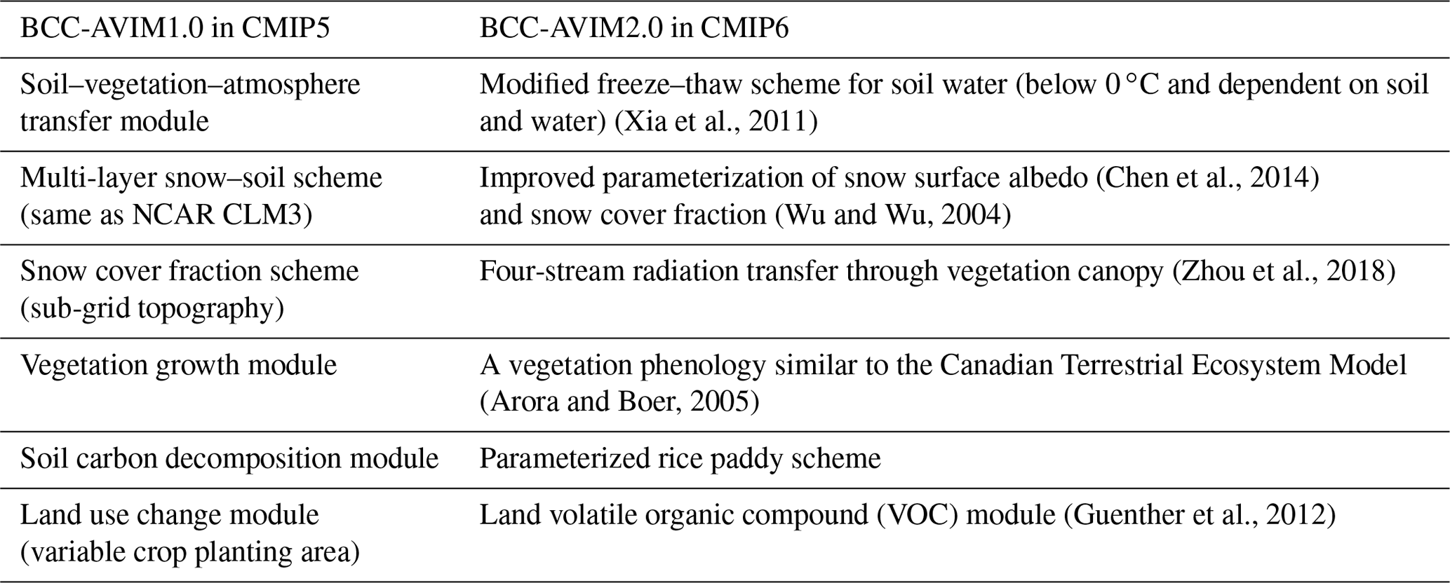
BCC-AVIM, the Beijing Climate Center Atmosphere–Vegetation Interaction Model, is a comprehensive land surface scheme developed and maintained in the BCC. Version 1 (BCC-AVIM1.0) was used as the land component in BCC-CSM1.1m, which participated in CMIP5 (Wu et al., 2013). It includes major land surface biophysical and plant physiological processes, and its origin could be traced back to the Atmosphere–Vegetation Interaction Model (AVIM) (Ji, 1995; Ji et al., 2008) with the necessary framework to include biophysical, physiological, and soil carbon–nitrogen dynamical processes. The biophysical module in BCC-AVIM1.0, with 10 layers for soil and up to 5 layers for snow, is almost the same as that used in the NCAR Community Land Model version 3 (CLM3) (Oleson et al., 2004). The terrestrial carbon cycle in BCC-AVIM1.0 consists of a series of biochemical and physiological processes modulating the photosynthesis and respiration of vegetation. Carbon assimilated by vegetation is parameterized by a seasonally varying allocation of carbohydrate to leaves, stem, and root tissues as a function of the prognostic leaf area index. Litter due to turnover and mortality of vegetation, and carbon dioxide release into the atmosphere via the heterogeneous respiration of soil microbes is taken into account in BCC-AVIM1.0. Vegetation litter falls to the ground surface and into the soil are divided into eight idealized terrestrial carbon pools according to the timescale of carbon decomposition of each pool and transfers among different pools, which are similar to those in the carbon exchange between vegetation, soil, and the atmosphere (CEVSA) model (Cao and Woodward, 1998).
BCC-AVIM1.0 has been updated to BCC-AVIM2.0 which serves as the land component of BCC-CSM2-MR, which participates in CMIP6. As listed in Table 3, several improvements have been implemented in BCC-AVIM2.0, such as the inclusion of a variable temperature threshold to determine soil water freezing–thawing rather than a fixed temperature of 0 ∘C, a better calculation of snow surface albedo and snow cover fraction, a dynamic phenology for deciduous plant function types, and a four-stream approximation of solar radiation transfer through vegetation canopy. Additionally, a simple scheme for surface fluxes over rice paddies is also implemented in BCC-AVIM2.0. These improvements are briefly discussed in the following.
- a.
Soil water freezes at a constant temperature of 0 ∘C in BCC-AVIM1.0, but the actual freezing–thawing process is a slow and continuously changing process. We take into account the fact that the soil water potential remains in equilibrium with the water vapor pressure over pure ice when soil ice is present. Based on the relationships among the soil water matrix potential ψ (mm), soil temperature and soil water content, a variable temperature threshold for freeze–thaw dependent on the soil liquid water content, the soil porosity, and the saturated soil matrix potential is introduced. The inclusion of this scheme improves the performance of BCC-AVIM2.0 in the simulation about seasonal frozen soil (Xia et al., 2011).
- b.
In BCC-AVIM1.0, we took the snow aging effect on surface albedo into account with a simple consideration using a unified scheme to mimic the snow surface albedo decrease with time. In BCC-AVIM2.0, we assume different reduction rates of snow albedo with actual elapsed time after snowfalls in the accumulating and melting stages of a snow season (Chen et al., 2014). Additionally, the variability of sub-grid topography is now taken into account to calculate the snow cover fraction within a model grid cell.
- c.
Unlike the empirical plant leaf unfolding and withering dates prescribed in BCC-AVIM1.0, a dynamic determination of leaf unfolding, growth, and withering dates according to the budget of photosynthetic assimilation of carbon similar to the phenology scheme in CTEM (Arora and Boer, 2005) was implemented in BCC-AVIM2.0. Leaf loss due to drought and cold stresses in addition to natural turnover are also considered.
- d.
The four-stream solar radiation transfer scheme within the canopy in BCC-AVIM2.0 is based on the same radiative transfer theory used in the atmosphere (Liou, 2004). It adopts the analytic formula of Henyey–Greenstein for the phase function. The vertical distribution of diffuse light within canopy is related to the transmissivity and reflectivity of leaves, in addition to the average leaf angle and the direction of incident direct beam radiation influence diffuse light within the canopy. The upward and downward radiative fluxes are determined by the phase function of diffuse light, the G-function, the leaf reflectivity and transmissivity, the leaf area index, and the cosine of the solar angle of incident direct beam radiation (Zhou et al., 2018).
- e.
Considering the wide distribution of rice paddies in Southeast Asia and the rather different characteristics of rice paddies and bare soil, a scheme to parameterize the surface albedo, roughness length, and turbulent sensible and latent heat fluxes over rice paddies is developed (a manuscript is currently in preparation) and implemented in BCC-AVIM2.0.
- f.
Finally, land use and land cover changes are explicitly involved in BCC-AVIM2.0. An increase in crop area implies the replacement of natural vegetation by crops, which is often known as deforestation.
2.3 Ocean and sea ice
There are no significant changes for the ocean and sea ice from BCC-CSM1.1m to BCC-CSM2-MR. However, for the sake of completeness, we present a short description of them here. The oceanic component is MOM4-L40, an oceanic GCM. It is based on the z coordinate Modular Ocean Model (MOM), version 4 (Griffies et al., 2005), developed by the Geophysical Fluid Dynamics Laboratory (GFDL). It has a nominal resolution of with a tri-pole grid, and the actual resolution is from latitude between 30∘ S and 30∘ N to 1.0∘ at 60∘ latitude. There are 40 z levels in the vertical. The two northern poles of the curvilinear grid are distributed to land areas over Northern America and over the Eurasian continent. There are 13 vertical levels placed between the surface and a depth of 300 m in the upper ocean. MOM4_L40 adopts some mature parameterization schemes, including Sweby's tracer-based third-order advection scheme, the isopycnal tracer mixing and diffusion scheme (Gent and McWilliams, 1990), the Laplace horizontal friction scheme, the KPP vertical mixing scheme (Large et al., 1994), the complete convection scheme (Rahmstorf, 1993), the overflow scheme of topographic processing of sea bottom boundary/steep slopes (Campin and Goosse, 1999), and the shortwave penetration schemes based on the spatial distribution of the chlorophyll concentration (Sweeney et al., 2005).
The concentration and thickness of sea ice are calculated using the Sea Ice Simulator (SIS) developed by the GFDL (Winton, 2000). The simulator is a global sea-ice thermodynamic model including the elastic–viscous–plastic dynamic processes and Semtner's thermodynamic processes. SIS has three vertical layers, including one snow cover and two ice layers of equal thickness. In each grid, five categories of sea ice (including open water) are considered, according to the thickness of sea ice. It also takes the mutual transformation from one category to another under thermodynamic conditions into account. The sea-ice model operates on the same oceanic grid and has the same horizontal resolution as MOM_L40. SIS calculates concentration, thickness, temperature, salinity of sea ice, and the motion of snow cover and ice sheets. There is no gas exchange through sea ice.
2.4 Surface turbulent fluxes between air and sea/sea ice
The atmosphere and sea/sea-ice interplay via the exchange of surface turbulent fluxes of momentum, heat, and water. An optimum treatment of the surface exchange, which is sound in physics and economic in computation, is very important in simulating the climate variability. Over the past several years, we have maintained a continuous effort to improve the turbulent exchange processes between air and sea/sea ice in different versions of the BCC models.
In BCC-CSM1.1m, the bulk formulas of turbulent fluxes over the sea surface originate from those used in CAM3, with some modifications to the roughness lengths and corrections to the temperature and moisture gradients considering sea-spray effects (Wu et al., 2010). The bulk formulas are updated in BCC-CSM2-MR. The coefficients of roughness length calculations were adjusted, and the arbitrary gradient corrections are not used. Instead, a gustiness parameterization is included to account for the sub-grid wind variability that is contributed by boundary layer eddies, convective precipitation, and cloudiness (Zeng et al., 2002).
In terms of turbulent exchange between air and sea ice, we proposed a new bulk algorithm that aims to improve flux parameterizations over sea ice (Lu et al., 2013). Based on theoretical and observational analysis, the new algorithm employs superior stability functions for stable stratification as suggested by Zeng et al. (1998), and features varying roughness lengths. All three roughness lengths (z0, zT, zQ) of sea ice were set to a constant (0.5 mm) in BCC-CSM1.1m. Observational studies show that values of z0 tend to be smaller than 0.5 mm over sea ice in winter and larger than 0.5 mm in summer (Andreas et al., 2010a, b). In the new parameterization used in BCC-CSM2-MR, the roughness lengths for momentum differentiate between warm and cold seasons. For simplicity, z0 is treated as
where Ts represents surface temperature. For the scalar roughness lengths, a theory-based model proposed by Andreas (1987) is used in the new scheme. This model expresses the scalar roughness zs (zT or zQ) as a function of the roughness Reynolds number R*, i.e.,
Andreas (1987, 2002) tabulates the polynomial coefficients b0, b1, and b2.
All BCC simulations presented in this work follow the protocols defined by CMIP5 and CMIP6. We aim for them to be comparable in spite of showing the transition of our climate system model from CMIP5 to CMIP6. The principal simulation to be analyzed is the historical simulation (hereafter historical) with prescribed forcings from 1850 to 2005 for CMIP5 (to 2014 for CMIP6).
Historical forcings data are based, as far as possible, on observations and were downloaded from (https://esgf-node.llnl.gov/search/input4mips/, last access: 1 April 2018). They mainly include the following: (1) GHG concentrations (only CO2, N2O, Ch4, CFC11, and CFC12 used in BCC models) with zonal-mean values which are updated monthly; (2) yearly global gridded land use forcing; (3) solar forcing; (4) stratospheric aerosols (from volcanoes); (5) CMIP6-recommended anthropogenic aerosol optical properties which are formulated in terms of nine spatial plumes associated with different major anthropogenic source regions (Stevens et al., 2017); and (6) time-varying gridded ozone concentrations. In addition, aerosol masses based on CMIP5 (Taylor et al., 2012) are used for the online calculation of the cloud droplet effective radius in the BCC model.
The preindustrial initial state of BCC-CSM2-MR is preceded by a 500-year piControl simulation following the requirement of CMIP6. The initial state of the piControl simulation itself is obtained via individual spin-up runs of each component of BCC-CSM2-MR in order for the piControl simulation to run stably and quickly to its model equilibrium. Actually, the initial states of atmosphere and land are obtained from a 10-year AMIP run forced with monthly climatology of sea surface temperature (SST) and sea-ice concentration, whereas the initial states of ocean and sea ice are derived from a 1000-year forced run with a repeating annual cycle of monthly climatology of atmospheric state from the Coordinated Ocean-ice Reference Experiment (CORE) data set version 2 (Danabasoglu et al., 2014). Figure 2 shows time series of the annual and global mean of the net energy flux at top-of-atmosphere (TOA) and the sea surface temperature for 600 years in the piControl simulation. The whole system in BCC-CSM2-MR fluctuates around a +0.4 W m−2 net energy flux at TOA without an obvious trend over 600 years. The global mean surface air temperature shows a small warming after 600 years (Fig. 2b). During the last 300 years, there are (±0.2 K amplitude) oscillations of centennial scale for the whole globe and for the areal average of 60∘ S to 60∘ N. These oscillations are certainly caused by the internal variation of the system.

Figure 2Time series of (a) the global mean net energy flux at top-of-atmosphere (W m−2) and (b) the global (black line) and regional (60∘ S to 60∘ N, red line) surface air temperature (∘C) for the 600 years of piControl simulations.
4.1 Global energy budget
Radiative fluxes at the top of the model atmosphere are fundamental variables characterizing the Earth's energy balance. Satellite observations in modern time allow us to monitor changes in the net radiation at top-of-atmosphere (TOA) from 2001 onwards. The CERES (Clouds and Earth's Radiant Energy System) project, with the lessons learned from its predecessor, the Earth's Radiation Budget Experiment (ERBE), provides improved observation-based data products of Earth's radiation budget (Wielicki et al., 1996). Recently, data of CERES have been synthesized with EBAF (Energy Balanced and Filled) data to derive the CERES-EBAF products, which are suitable for the evaluation of climate models (Loeb et al., 2012). As shown in Table 4, the TOA shortwave and longwave components in BCC-CSM2-MR are generally closer to CERES-EBAF than those in BCC-CSM1.1m. Model results are for the 1986–2005 period, whereas the available CERES-EBAF data are for the 2003–2014 period. Globally averaged TOA net energy is 0.85 W m−2 in BCC-CSM2-MR and 0.98 W m−2 in BCC-CSM1.1m for the period from 1986 to 2005. The energy equilibrium of the whole Earth system in BCC-CSM2-MR is slightly improved.
Table 4Energy balance and cloud radiative forcing at the top-of-atmosphere (TOA) in the model with contrast to CERES-EBAF and CERES observations. (Units: W m−2.)
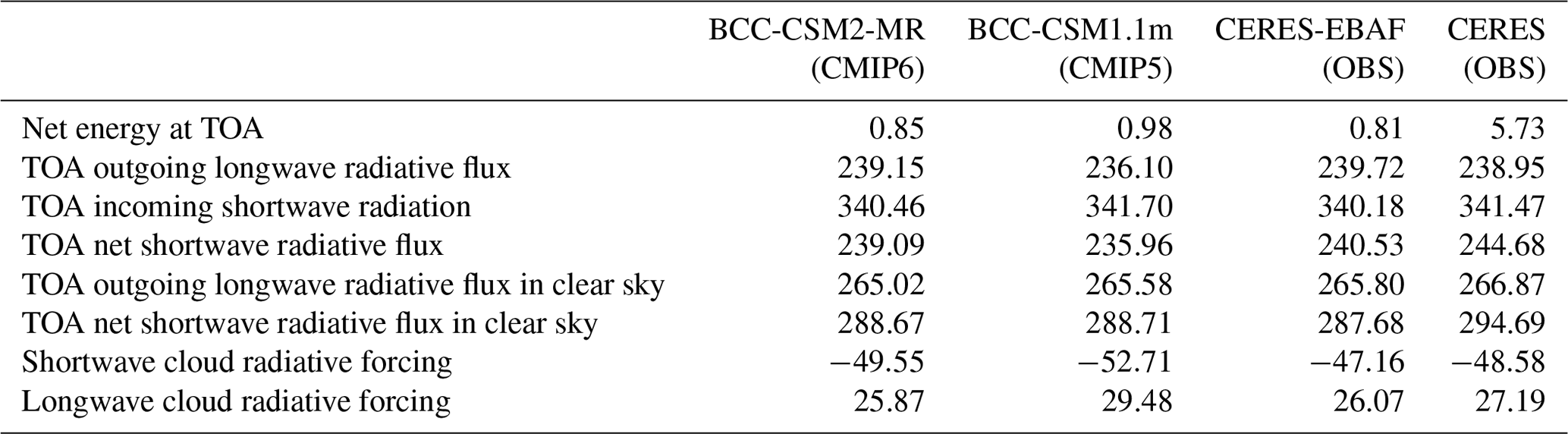
Notes: the model data are the mean of 1986–2005, whereas the available observation data are for 2003–2014.
Clouds constitute a major modulator of the radiative transfer in the atmosphere for both solar and terrestrial radiations. Their macro and micro properties, including their radiative properties, exert strong impacts on the equilibrium and variation of the radiative budget at TOA or at the surface. Figure 3 displays the annual and zonal means of shortwave, longwave, and net cloud radiative forcing for the BCC CMIP5 models (blue curves), the BCC CMIP6 (red curves) models, and the observations (black curves). The data used in Fig. 3 are the same as in Table 4. Although observations and models results cover different time periods, they are still relevant to reveal climatological mean performance of climate models. At low latitudes between 30∘ S and 30∘ N, BCC-CSM1.1m shows excessive cloud radiative forcing for both shortwave and longwave radiation. These biases are largely reduced in BCC-CSM2-MR, which is possibly attributed to the new cloud fraction algorithm especially for convective cloud amount. Cloud radiative forcing at midlatitudes shows large uncertainty, which is also manifested in the large deviation between the two observations. Cloud radiative forcing in both models is closer to CERES-EBAF than to CERES at midlatitudes. It is clear that the new physics modifies the simulated climate and cloud properties, including the fractional coverage of clouds, their vertical distribution, and their liquid water and ice content.
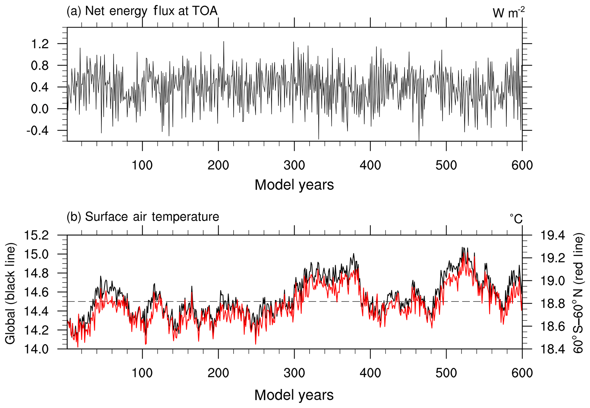
Figure 3Zonal averages of the cloud radiative forcing (CRF) from the BCC CMIP5 and CMIP6 models and the observations (in W m−2; a: shortwave effect; b: longwave effect; c: net effect). Model results are for the 1986–2005 period, whereas the available CERES ES-4 and CERES-EBAF 2.6 data set are for the 2003–2014 period.
4.2 Performance simulating the global warming in the 20th century
The historical simulation allows us to evaluate the ability of models to reproduce the global warming and climate variability in the 20th century. The performance depends on both the model formulation and the time-varying external forcings imposed on the models (Allen et al., 2000). Figure 4 presents global-mean (from 60∘ S to 60∘ N) surface air temperature evolutions from HadCRUT4 (Morice et al., 2012) and the BCC CMIP5 and CMIP6 models. In this study, only the area from 60∘ S to 60∘ N is used for comparison, as few observations exist in polar regions to deduce reliable information in HadCRUT4, especially before the 20th century. To better reveal long-term trends, the climatological mean is calculated for the reference period from 1961 to 1990 and is removed from the time series. The interannual variability of both simulations is qualitatively comparable to that observed. When an 11-year smoothing is applied, the long-term trend of both the CMIP6 and CMIP5 models is highly correlated with HadCRUT4. Figure 4 presents three members of historical simulations from different initial states of the piControl simulation. The correlation coefficients are 0.90 in CMIP5 and 0.93, 0.93, and 0.90 in the three members of CMIP6, respectively.
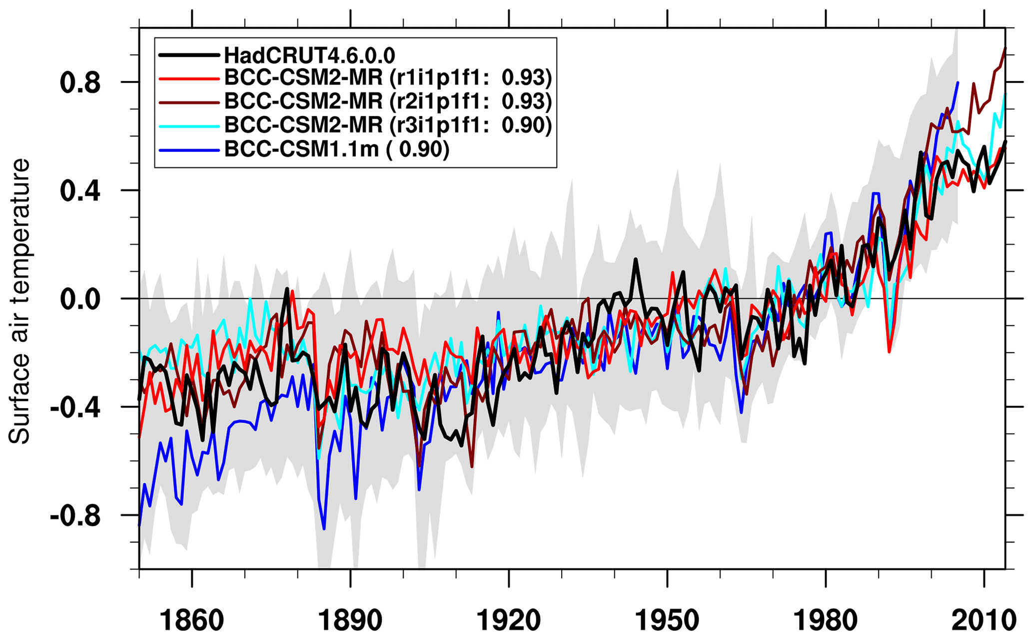
Figure 4Time series of anomalies in the global (60∘ S to 60∘ N) mean surface air temperature from 1850 to 2014. The reference climate to deduce anomalies is from 1961 to 1990 for each individual curve. The three lines labeled BCC-CSM2-MR denote the three members of the historical simulations from different initial states of the piControl simulation. The numbers in parentheses denote the correlation coefficient of the 11-year smoothed BCC model data with the HadCRUT4.6.0.0 (Morice et al., 2012) observations. The gray shaded area shows the spread of the 36 CMIP5 models' data.
A remarkable feature in Fig. 4 is the presence of a global warming hiatus or pause for the period from 1998 to 2013 when the observed global surface air temperature warming slowed down. This is a hot topic, which is largely debated in the scientific research community (e.g., Fyfe et al., 2016; Medhaug et al., 2017). Two members (r1i1p1f1 and r2i1p1f1 in Fig. 4) of the historical simulations of the CMIP6 model show a hiatus towards the end of the simulation that resembles the observed pause. Although the third member (r3i1p1f1) simulated a global warming slowdown from 2004 to 2012, it is not comparable to the observed hiatus, as it has a short spell of colder years centered on 2010. Another warming hiatus occurred during the period from 1942 to 1974. The first and the third members (r1i1p1f1 and r3i1p1f1) of BCC-CSM2-MR only simulate the warming slowdown in the late period from 1958 to 1974, but the second member (r2i1p1f1) of BCC-CSM2-MR almost simulates this warming hiatus throughout the period from 1942 to 1974. Therefore, the simulation of a global warming hiatus in the BCC CMIP6 model clearly excludes any simple response to forcing, and makes internal variability a much more likely reason.
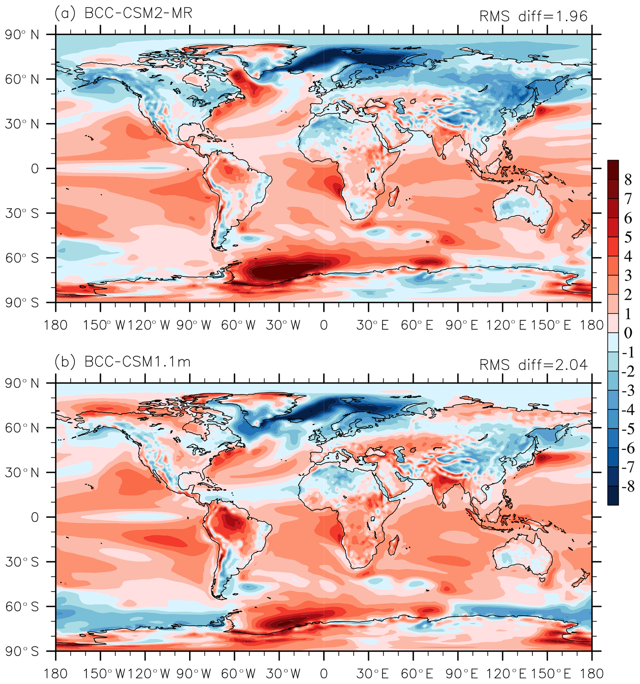
Figure 5Annual-mean surface (2 m) air temperature biases (∘C) of (a) BCC-CSM2-MR and (b) BCC-CSM1.1m simulations contrasted with the ERA-Interim reanalysis for the period from 1986 to 2005.
The model response of the surface air temperature (SAT) to volcanic forcing is slightly stronger than that estimated with HadCRU data. Evident global cooling shocks are coincident with significant volcanic eruptions such as Krakatoa (in 1883), Mount Agung (in 1963), and Mount Pinatubo (in 1991). Each of these volcanic eruptions significantly enriched stratospheric aerosols (available from http://data.giss.nasa.gov/modelforce/strataer/, last access: 5 January 2017). As shown in Fig. 4, SAT may decrease by up to 0.4 ∘C within 1 to 2 years after major volcanic eruptions. The substantial cooling response to volcanic eruptions is, to a great extent, due to an overly strong aerosol direct radiative forcing in both versions of the BCC-CSM.
To keep the paper concise and of a reasonable length, only the first member of the CMIP6 historical simulations of BCC-CSM2-MR will be presented hereafter. Biases of the annual-mean surface air temperature (at 2 m) over the whole globe for BCC-CSM2-MR and BCC-CSM1.1m are shown in Fig. 5. In both BCC models, biases are generally within ±3 ∘C, but there are slight systematic warm biases over oceans from 50∘ S to 50∘ N and systematic cold biases over most land regions north of 50∘ N, in East Asia and northern Africa. Cold biases at high latitudes in the Northern Hemisphere (North Atlantic, Arctic, North America, and Siberia) seem amplified in BCC-CSM2-MR. The land surface biases in both coupled models are similar to one another. These patterns of biases are already present in AMIP simulations (not shown), where the effects of oceanic biases are excluded. Hence, these biases in land surface partly come from their land surface modeling component. In the Southern Ocean, both models show a strong warm area in the Weddell Sea. BCC-CSM1.1m shows cold biases in other regions of the Southern Ocean. The disappearance of cold biases in the Southern Oceans in BCC-CSM2-MR is possibly due to the new scheme for the cloud fraction (Table 2), as there is a zone of low-level cloud between 40 and 60∘ S in the Southern Ocean (omitted), not only in the models but also in observations.
4.3 Climate sensitivity to increasing CO2
The long trend of global warming in Fig. 4 depends on the climate sensitivity which is an emblematic parameter to characterize the sensitivity of a climate model to external forcing, with all feedbacks included. It generally designates the variation of the global mean surface air temperature in response to a forcing of doubled CO2 concentration in the atmosphere (IPCC, 2013). As commonly practiced in the climate modeling community, an equilibrium climate sensitivity and a transient climate response can be separately evaluated, corresponding to a situation of equilibrium and transient states of climate.
We use the standard simulation of 1 % CO2 increase per year (1pctCO2) to calculate the transient climate response (TCR), whereas the equilibrium climate sensitivity (ECS) uses the 4× CO2 abrupt-change simulation by applying the forcing/response regression methodology proposed by Gregory et al. (2004). The TCR is calculated using the difference of the annual surface air temperature between the preindustrial experiment and a 20-year period centered on the time of CO2 doubling in 1pctCO2, which is 1.71 for BCC-CSM2-MR and 2.02 for BCC-CSM1.1m. The ECS is diagnosed from the 150-year run of abrupt 4× CO2 following the approach of Gregory et al. (2012). The method is based on the linear relationship (Fig. 6) governing the changes of the net top-of-atmosphere downward radiative flux and the surface air temperature simulated in abrupt 4× CO2 relative to the preindustrial experiment. The ECS is equal to a half of the temperature change when the net downward radiative flux reaches zero (Andrews et al., 2012). It is assumed here that 2× CO2 forcing is half of that for 4× CO2, a hypothesis which is generally verified in climate models. As shown in Fig. 6, the ECS is 3.03 for BCC-CSM2-MR and 2.89 for BCC-CSM1.1m. Therefore, the TCR of the new version model BCC-CSM2-MR is lower than BCC-CSM1.1m, but the ECS of BCC-CSM2-MR is slightly higher than BCC-CSM1.1m.

Figure 6Relationships between the change in the net top-of-atmosphere radiative flux and the global-mean surface air temperature change simulated with an abrupt 4× CO2 increase relative to the preindustrial control run.
The linear regression line shown in Fig. 6, as pointed out in Gregory et al. (2012), also allows for the estimation of the instantaneous forcing due to CO2 increase, and eventually of the feedback parameter on the climate system. The former is the cross point of the linear regression line with y axis: 6.2 W m−2 for BCC-CSM2-MR and 7.6 W m−2 for BCC-CSM1.1m. They can be scaled to the case of 2× CO2 using a division factor of 2. As the ECS values are close to each other in the two models, we can easily deduce that the all-feedback factor is larger in BCC-CSM2-MR than in BCC-CSM1.1m. It is actually not surprising to see differences of 2× CO2 radiative forcing between the two models even if the radiative transfer scheme is kept identical, because changes in the 3-D structures of cloud, the atmospheric temperature, and water vapor do exert impacts on additional radiative forcing due to CO2 increase in the atmosphere. However, it is interesting to note that feedbacks can operate in such different ways in the two models that the ECS remains almost unchanged between them. We remind the reader that this is pure coincidence, as we did not intentionally tune our model for its sensitivity.
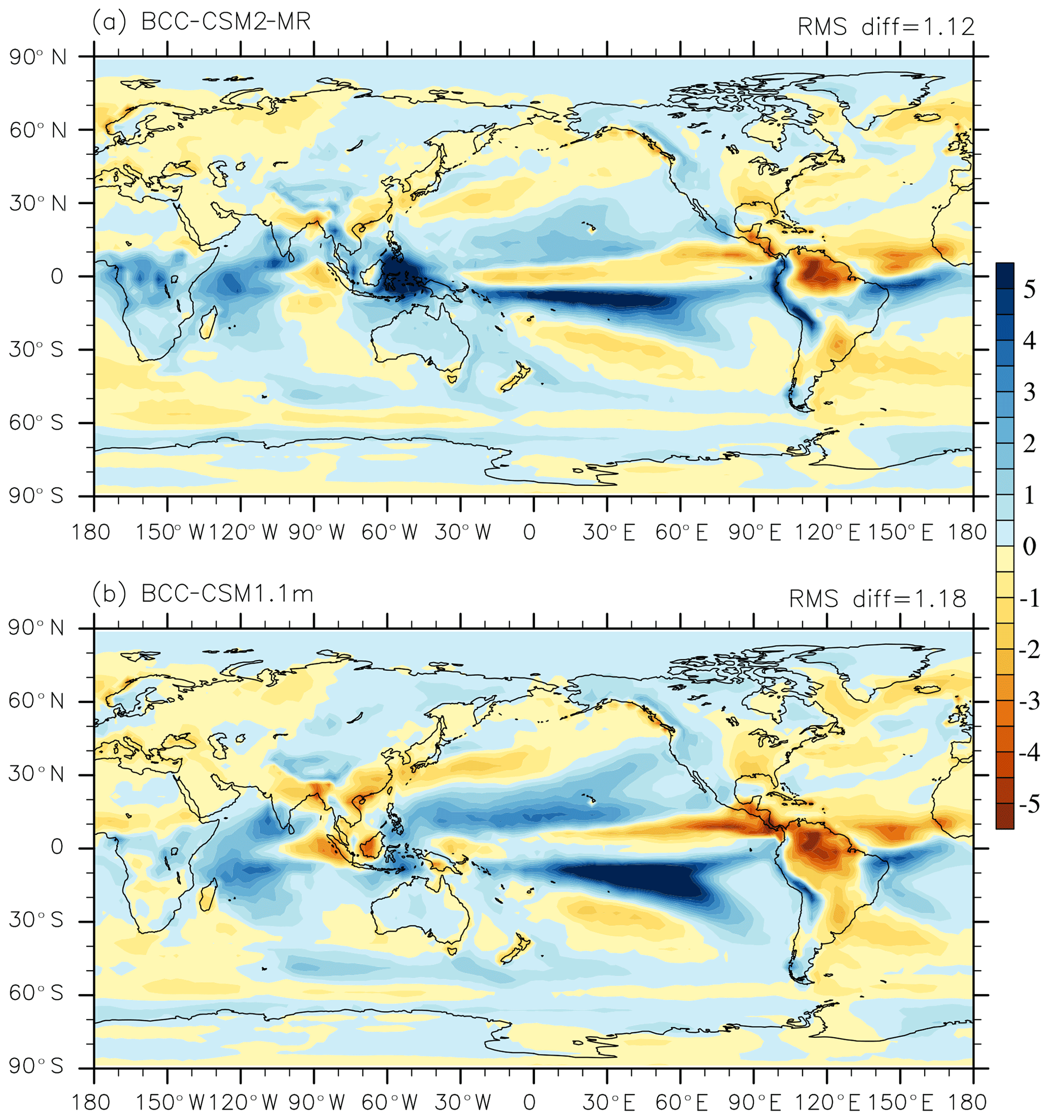
Figure 7Annual-mean precipitation rate biases (mm d−1) of (a) BCC-CSM2-MR and (b) BCC-CSM1.1m simulations in contrast with the 1986–2005 precipitation analyses from the Global Precipitation Climatology Project (Adler and Chang, 2003).
4.4 Present-day behaviors of the atmosphere
The main spatial patterns of observed precipitation climatology are simulated in BCC-CSM1.1m and BCC-CSM2-MR. Figure 7 shows model biases of annual-mean precipitation for BCC-CSM1.1m and BCC-CSM2-MR around the globe. They are very close to one another; their RMSE is also very close: 1.12 mm d−1 against 1.18 mm d−1. Regions that display a lack of precipitation, such as northern India, southern China, the two sides of Sumatra, and the Amazon, experience significant amelioration in the new model. Excessive rainfall in tropical Africa, in the Indian Ocean, and in the Maritime Continent region seem amplified in BCC-CSM2-MR. As for the whole globe, the annual mean precipitation coming from convective process (including deep and shallow convections) accounts for 50 % of the total precipitation (2.94 mm d−1) in BCC-CSM2-MR and 48 % of the total precipitation (2.87 mm d−1) in BCC-CSM1.1m. The convective precipitation increases in BCC-CSM2-MR, and the total amount of precipitation exceeds the amount (2.68 mm d−1) of the 1986–2005 mean observed precipitation analyses from Global Precipitation Climatology Project (Adler and Chang, 2003). However, in some regions such as the Maritime Continent, stratus precipitation evidently enhances in BCC-CSM2-MR, where the ratio of convection precipitation to total precipitation is 39 % and even higher than 35 % in BCC-CSM1.1m.
We now use the Taylor diagram (Fig. 8) to evaluate the general performance of our two models in terms of temperature at 850 hPa, precipitation, and atmospheric general circulation. The evaluation is carried out against the climatology of the ERA-Interim data set for the period from 1986 to 2005 (Dee et al., 2011). ERA-Interim is the latest global atmospheric reanalysis produced by the European Centre for Medium-Range Weather Forecasts (ECMWF).
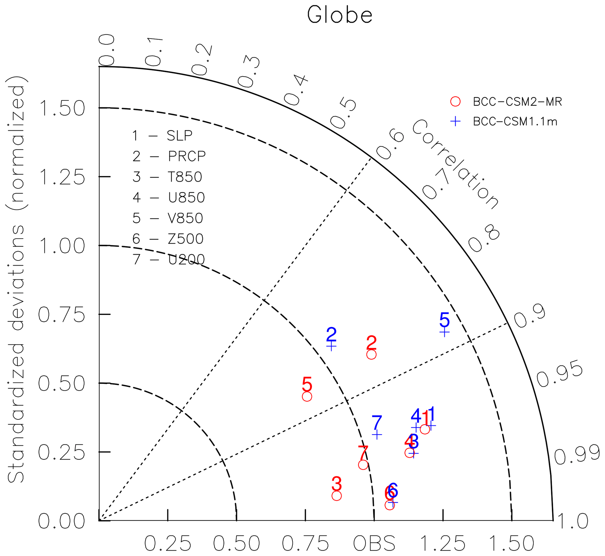
Figure 8Taylor diagram for the global climatology (1980–2005) of sea level pressure (SLP), precipitation (PRCP), temperature at 850 hPa (T850), zonal wind at 850 hPa (U850), longitudinal wind at 850 hPa (V850), geopotential height at 500 hPa (Z500), and zonal wind at 200 hPa (U200). The radial coordinate shows the standard deviation of the spatial pattern, normalized by the observed standard deviation. The azimuthal variable shows the correlation of the modeled spatial pattern with the observed spatial pattern. The analysis is for the whole globe. The reference data set is ERA-Interim except for the precipitation from the Global Precipitation Climatology Project data set. The model results of BCC-CSM2-MR and BCC-CSM1.1m are the mean for the 1980–2000 period. Blue crosses represent BCC-CSM1.1m, and circles represent BCC-CSM2-MR.
For global fields, we calculate the spatial pattern correlations between models and ERA-Interim for the annual-mean climatology of sea level pressure (SLP), temperature at 850 hPa level (T850), zonal and meridional wind velocity at 850 hPa (U850 and V850), zonal wind velocity at 200 hPa (U200), geopotential height at 500 hPa (Z500), and precipitation from the Global Precipitation Climatology Project (PRCP in Fig. 8, Adler and Chang, 2003) over the period 1980–2000. Except for PRCP and U850, which have a lower correlation (less than 0.90) with the observations, other variables are have correlation coefficients above 0.90. The pattern correlation coefficient of Z500 with ERA-Interim is 0.995, which is the best correlation among these variables. Except for V850, correlations of all other variables in the CMIP6 model version (BCC-CSM2-MR) show an evident improvement compared with the CMIP5 version (BCC-CSM1.1m). The normalized standard deviations of most variables except for PRCP and T850 are obviously improved in BCC-CSM2-MR. As a whole, the performance of most variables in BCC-CSM2-MR is better than those in BCC-CSM1.1m.
Results shown in the Taylor diagrams in Fig. 8 regarding improvements in surface climate and atmospheric general circulation at different vertical levels are consistent with improvements in the vertical distribution of atmospheric temperature. Figure 9 shows the yearly averaged zonal mean of atmospheric temperature biases in BCC-CSM2-MR and BCC-CSM1.1m, with ERA-Interim for the period from 1986 to 2005 as a reference. Overall, both BCC-CSM2-MR and BCC-CSM1.1m have similar biases in their vertical structure: they are 1–3 K warmer in the stratosphere (above 100 hPa) for most of the domain equatorward of 70∘ N and 70∘ S. There are larger cold biases near the tropopause (centered near 200 hPa) for southward of 30∘ S and northward of 30∘ N. In the middle to lower troposphere (below 400 hPa), there is a warm bias of 1–2 K. Improvements in BCC-CSM2-MR are mainly located in the troposphere below 100 hPa. Both cold biases near the tropopause at high latitudes and warm bias at lower latitudes are reduced.
The improvement in tropospheric temperature induces naturally smaller biases for the zonal wind throughout the troposphere in BCC-CSM2-MR (Fig. 9). However, there are still westerly wind biases of 6 m s−1 in the 100–200 hPa layer in the tropics. Westerly jets at midlatitudes are slightly too strong in both hemispheres. The zonal mean of zonal wind biases at high latitudes of the stratosphere in BCC-CSM2-MR increase near 10 hPa. The overly strong polar night jets clearly indicate an insufficient atmospheric drag at this level. This may be partly caused by the lack of effects in relation to some non-orographic gravity waves generated by atmospheric fronts and jets. We expect to reduce this model bias in next version by adding this process.
Given a much higher vertical resolution and an advanced parameterization of the gravity wave drag, the new model BCC-CSM2-MR is able to represent the stratospheric quasi-biennial oscillation (QBO), as shown in Fig. 10 which displays time–height diagrams of the tropical zonal winds averaged from 5∘ S to 5∘ N. The three panels show observations from the ERA-Interim reanalysis and relevant simulation results from the two models in CMIP6 and CMIP5. Figure 10a shows alternative westerlies and easterlies in the lower stratosphere appearing with a mean period of about 28 months in the ERA-Interim reanalysis. In Fig. 10b, the BCC-CSM2-MR simulations present a clear quasi-biennial oscillation of the zonal winds as observed. In this study, the QBO period is taken as the time between easterly and westerly wind transitions at 20 hPa. The simulation produces about 12 QBO cycles from 1980 to 2005. The average period is 24.6 months, whereas the shortest and longest cycles last for 18 and 35 months, respectively. ERA-Interim values are 27.9, 23, and 35 months for the average, minimum, and maximum of the cycle length. The observed asymmetry in amplitude – with the easterlies being stronger than the westerlies – is reproduced in the simulated zonal winds. At 20 hPa, the simulated easterlies often exceed −20 m s−1, whereas in the reanalysis easterly winds peak at −30 to −40 m s−1. Simulated westerlies of the QBO range from 8 to 12 m s−1, whereas the reanalysis shows peak winds of 16 to 20 m s−1. The amplitudes of the QBO cycles in the simulation are weaker than in the reanalysis, which is possibly due to inadequate gravity wave forcing to drive the QBO. We suspect that the wave–mean flow interaction based on resolved waves such as Kelvin waves and mixed Rossby–gravity waves is probably not performant enough in BCC-CSM2-MR. One reason that would contribute to such a discrepancy is the relatively coarse vertical resolution (Table 1), which would affect the vertical wave lengths and the wave damping process. The downward propagation of the simulated QBO phases occurs in a regular manner, but does not penetrate to sufficiently low altitudes. It may depend on the vertical resolution, and the impact of the vertical resolution on downward propagation will be discussed in a separate paper. After a few test of model vertical layers, we tend to conclude that 46 seems to be the minimum number of layers required to simulate the QBO in BCC-CSM2-MR (Fig. 1). However, in BCC-CSM1.1m, as shown in Fig. 10c, the QBO is nonexistent and only a semiannual oscillation of easterlies can be found.
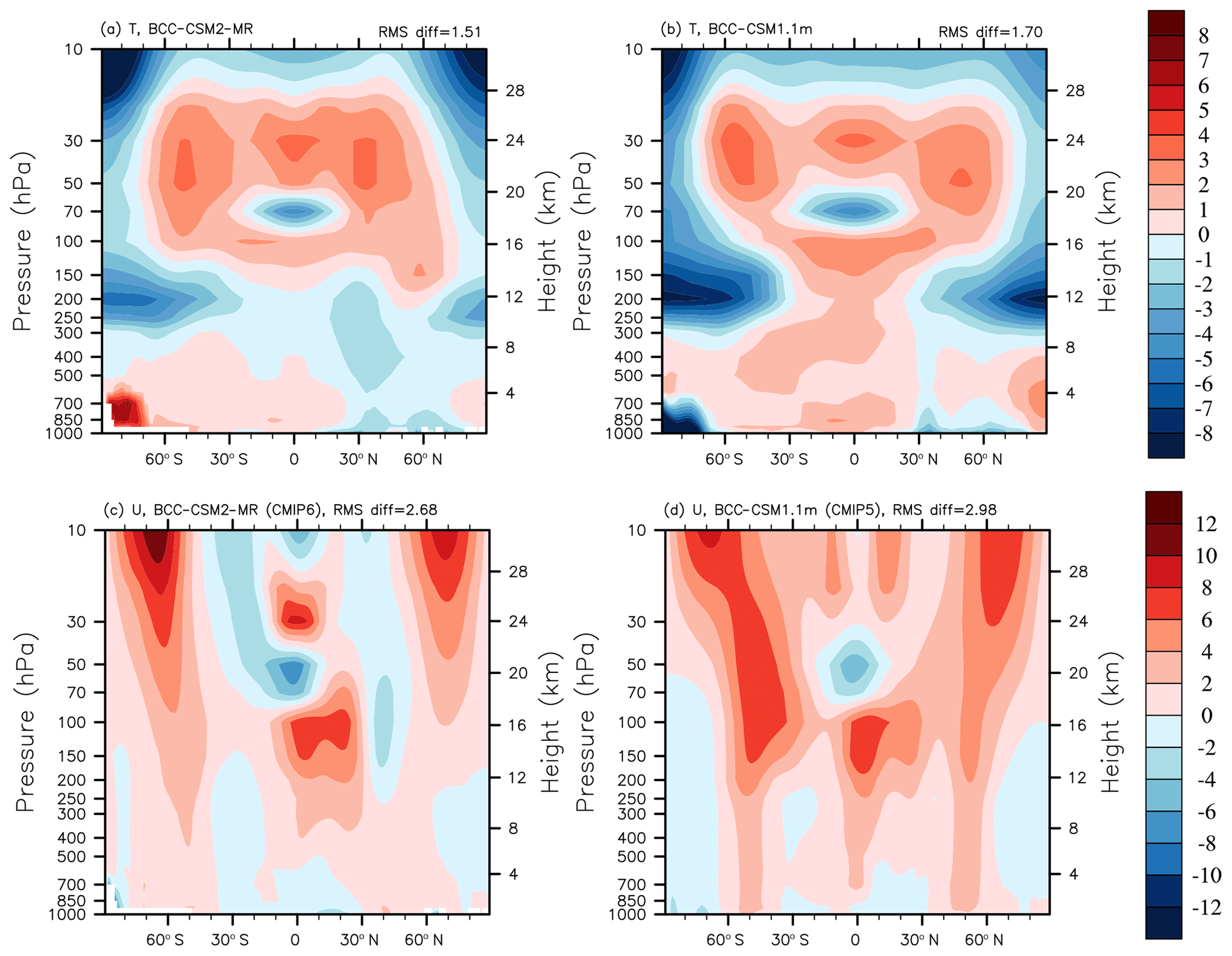
Figure 9Pressure–latitude sections of (a, b) annual mean temperature biases (in Kelvin) and (c, d) zonal wind biases (m s−1) for BCC-CSM2-MR (a, c) and BCC-CSM1.1m (b, d), with respect to the ERA-Interim reanalysis data for the period from 1986 to 2005.
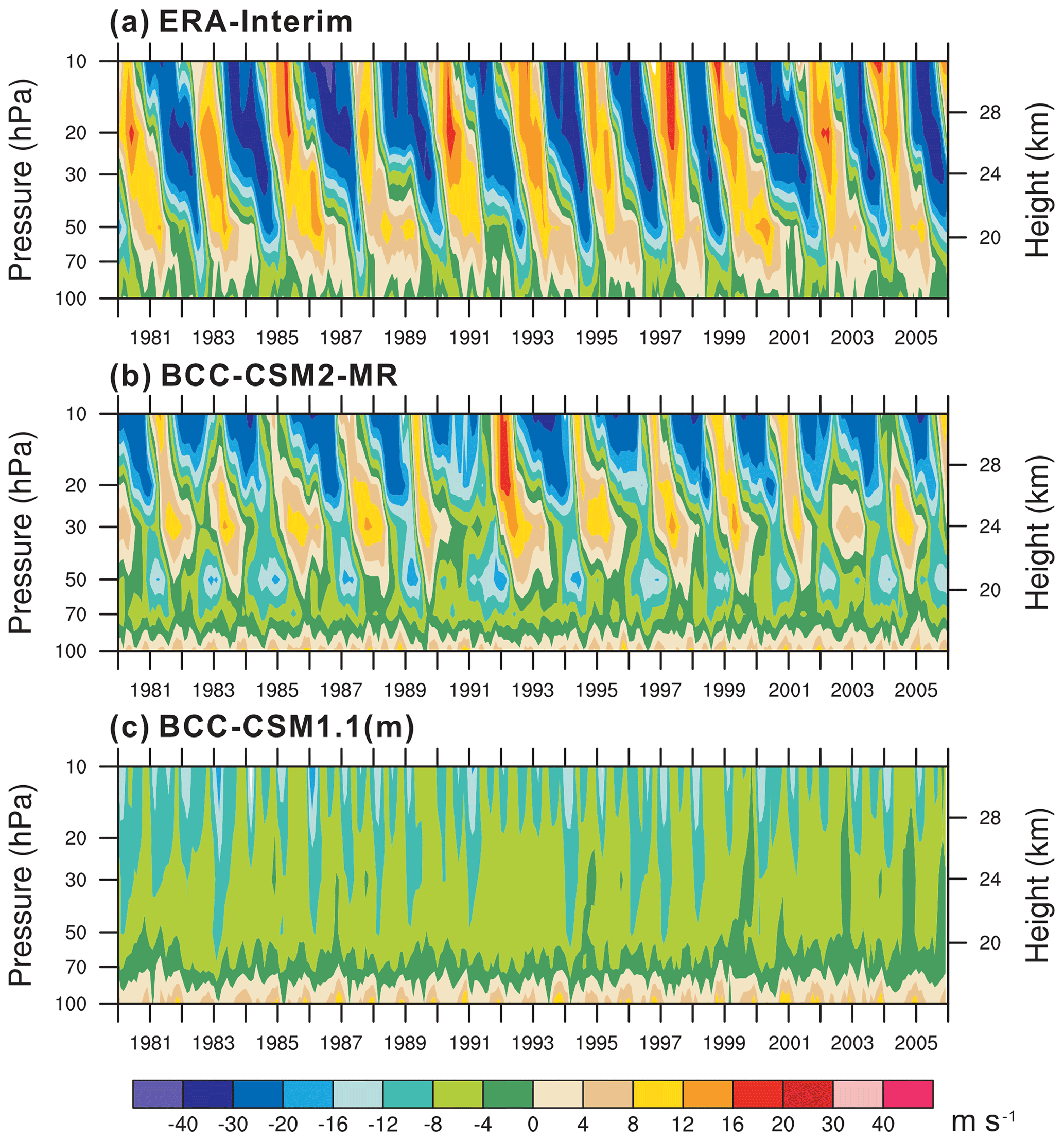
Figure 10Tropical zonal winds (m s−1) between 5∘ S and 5∘ N in the lower stratosphere from 1980 to 2005 for (a) ERA-Interim reanalysis, (b) BCC-CSM2-MR, and (c) BCC-CSM1.1m.
The Madden–Julian Oscillation (MJO) is a very important atmospheric variability acting within a periodicity between 20 and 100 d in the tropics with considerable effects on regional weather and climate. It exerts significant impacts on monsoonal circulations and the organization of tropical rainfall. From the tropical Indian Ocean to the western Pacific, the MJO shows a pronounced behavior of eastward propagation, as seen in Fig. 11a, in the form of longitude–time, the lagged correlation coefficient of the rainfall in the eastern Indian Ocean (75–85∘ E; 5∘ S–5∘ N) with other positions, and with lagged time. We can easily observe the eastward-propagating characteristic, with a moving velocity estimated at 5 m s−1. For the sake of comparison, the study of Jiang et al. (2015) shows that three-quarters of CMIP5 models do not show the propagation behavior, with only a standing oscillation when data are filtered to retain just the 20–100 d variability. Figure 11b and c show the same plot, but from our two models in CMIP5 and CMIP6. Although the new model is far from realistic in terms of eastward propagation, there is indeed a clear improvement compared with the old model.
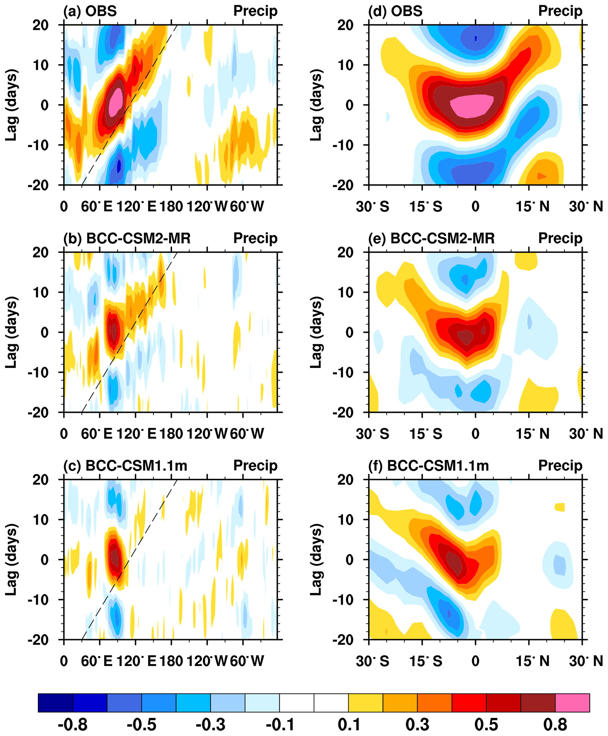
Figure 11(a, b, c) Longitude–time evolution of lagged correlation coefficients for the 20–100 d band-pass-filtered anomalous rainfall (averaged over 10∘ S–10∘ N) against itself averaged over the equatorial eastern Indian Ocean (75–85∘ E; 5∘ S–5∘ N). (d, e, f) Same as in (a, b, c) but to show the meridional propagation of the filtered rainfall, and lagged correlation coefficient for anomalous rainfall (averaged over 80–100∘ E) against the rainfall averaged over the same region of the equatorial eastern Indian Ocean. Dashed lines in each panel denote the 5 m s−1 eastward propagation speed. The reference GPCP observations and historical simulations of models are from the period from 1997 to 2005.
The MJO can also exert impacts on the weather and climate of the extra-tropics, either through the emanation of Rossby waves, or the poleward propagation of the MJO itself. Figure 11d shows a latitude–time diagram for lagged correlation coefficients when rainfalls are filtered to retain only the 20–100 d variability. Panels (e) and (f) in Fig. 11 are the counterparts simulated by our two models. The new model presents a clear improvement.
4.5 Interannual variation of sea surface temperature (SST) in the equatorial Pacific
Figure 12 shows the observed and simulated spatial pattern of the standard deviation of SST anomalies in the tropical Pacific. Both BCC-CSM2-MR and BCC-CSM1.1m can simulate the position of the strongest variation of SST, situated in the central-eastern Pacific – east of the dateline. However, cold SSTs in the eastern equatorial Pacific still extends too far west in both models, and a cold tongue bias exists in the equatorial Pacific and even gets a little worse in BCC-CSM2-MR. The annual mean SST in the coldest center near 110∘ W in the equatorial Pacific is below 23∘ in BCC-CSM2-MR, which is a deterioration compared with BCC-CSM1.1m. As shown in Fig. 12a, HadISST observations (Rayner et al., 2003) can clearly identify a zone of large interannual variation in the SST from the Peruvian coast to the equatorial cold tongue. It is well simulated in BCC-CSM2-MR, but almost missing in BCC-CSM1.1m.
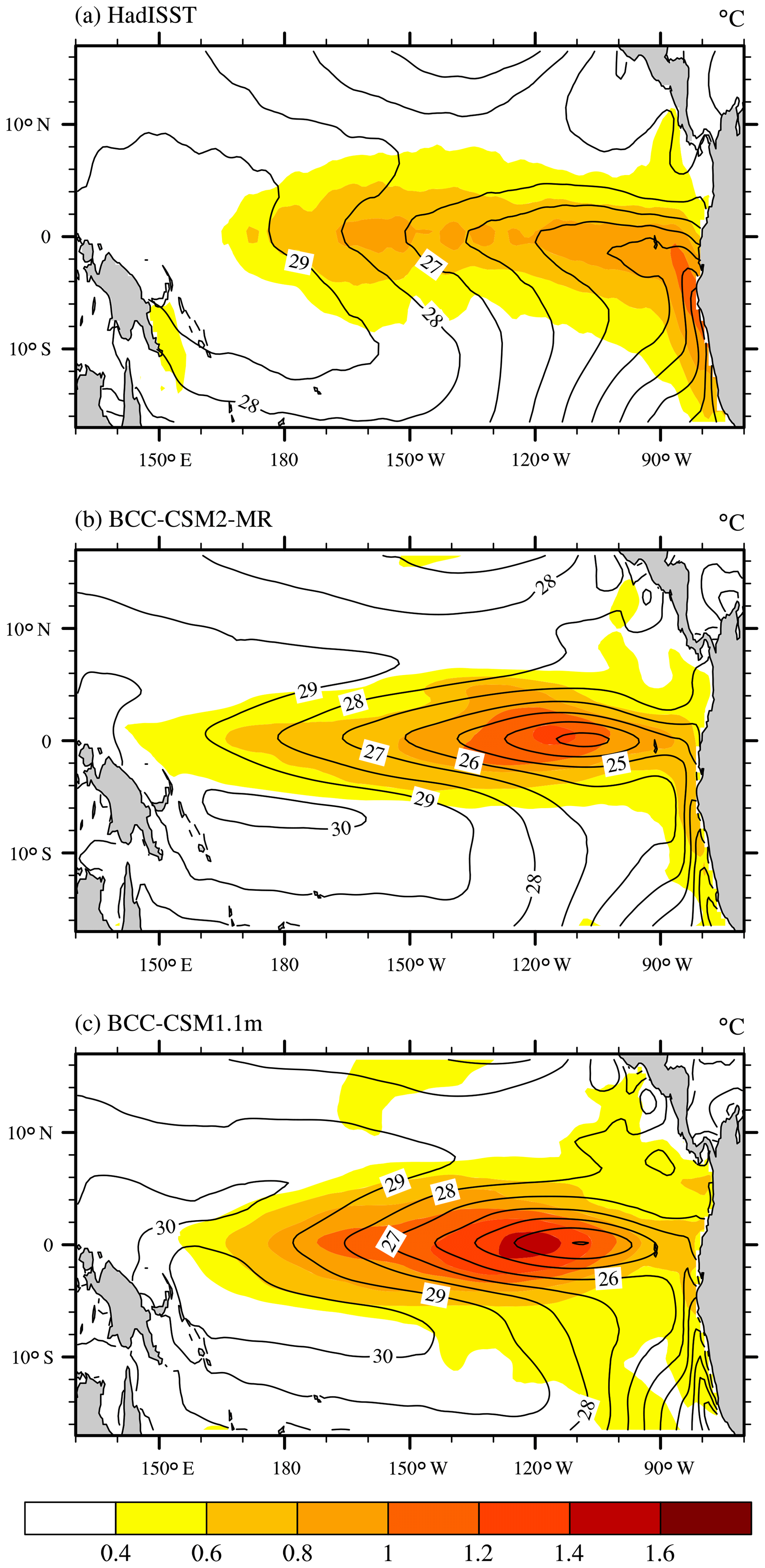
Figure 12The spatial distributions of the 1986–2005 annual mean sea surface temperature (contour lines, ∘C) and the standard deviations of the interannual anomalies (shaded area, ∘C) in the tropical Pacific for (a) HadISST observations (Rayner et al., 2003), (b) BCC-CSM2-MR, and (c) BCC-CSM1.1m.
Figure 13 presents time series of the monthly Nino3.4 SST index from observations and from simulations of BCC-CSM1.1m and BCC-CSM2-MR. Although amplitudes of interannual variations of the Nino3.4 index in both models are larger than in HadISST observations, it becomes weaker in BCC-CSM2-MR with a standard deviation of 0.91 ∘C, which is close to the observations that show a standard deviation of 0.79 ∘C. A recent studies from Lu and Ren (2016) revealed that the mean period El Niño–Southern Oscillation (ENSO) in BCC-CSM1.1m is only 2.4 years, which is much shorter than that seen in the observations. This bias of an overly short periodicity of the ENSO cycle still persists in BCC-CSM2-MR. Nevertheless, the characteristic of ENSO irregularity is improved in BCC-CSM2-MR in comparison with BCC-CSM1.1m.
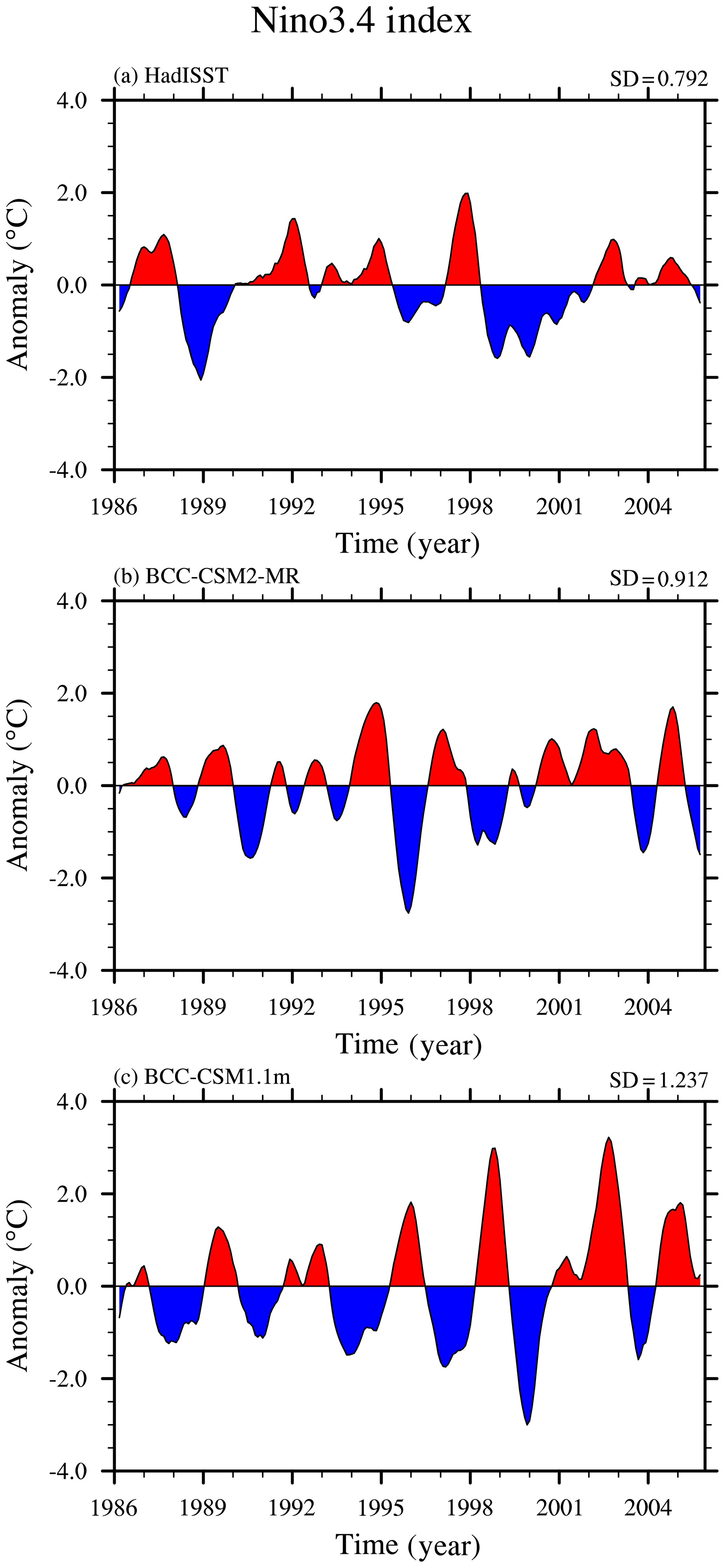
Figure 13The time series of the Nino3.4 SST index from 1986 to 2005 for (a) HadISST data, (b) BCC-CSM2-MR, and (c) BCC-CSM1.1m.
4.6 Sea-ice state and oceanic overturning circulation
Figure 14 shows time series of minimum sea-ice extent from 1851 to 2012 for (a) the Arctic in September and (b) the Antarctic in March as simulated in BCC-CSM2-MR and BCC-CSM1.1m. Based on the Hadley Centre Sea Ice and Sea Surface Temperature data set (Rayner et al., 2003, shown by “Hadley” in Fig. 14), the observed minimum sea-ice extent in each September from 1851 to 2012 gradually shrinks, especially since the 1960s, which is attributed to global warming (Fig. 4). The extent of Arctic sea ice in September in BCC-CSM1.1m is about 2×10⁶ km2 smaller than the Hadley Centre data, and it begins to shrink in the 1910s, which is earlier than in the observations. Although the Arctic sea-ice extent in September in BCC-CSM2-MR is even smaller than in BCC-CSM1.1m, the model performance is improved from the 1960s to present and is closer to the Hadley observation. In Fig. 14b, it can be noted that the Antarctic minimum sea-ice extent in the new model is very small, almost a half of what is observed. However, the old model had more realistic behavior in this regard. This discrepancy is related to overly warm temperatures simulated in BCC-CSM2-MR in the Southern Ocean, in particular in the Weddell Sea. The decreasing trend in the Arctic summer sea-ice extent is, however, better simulated in the new model than in the old one.
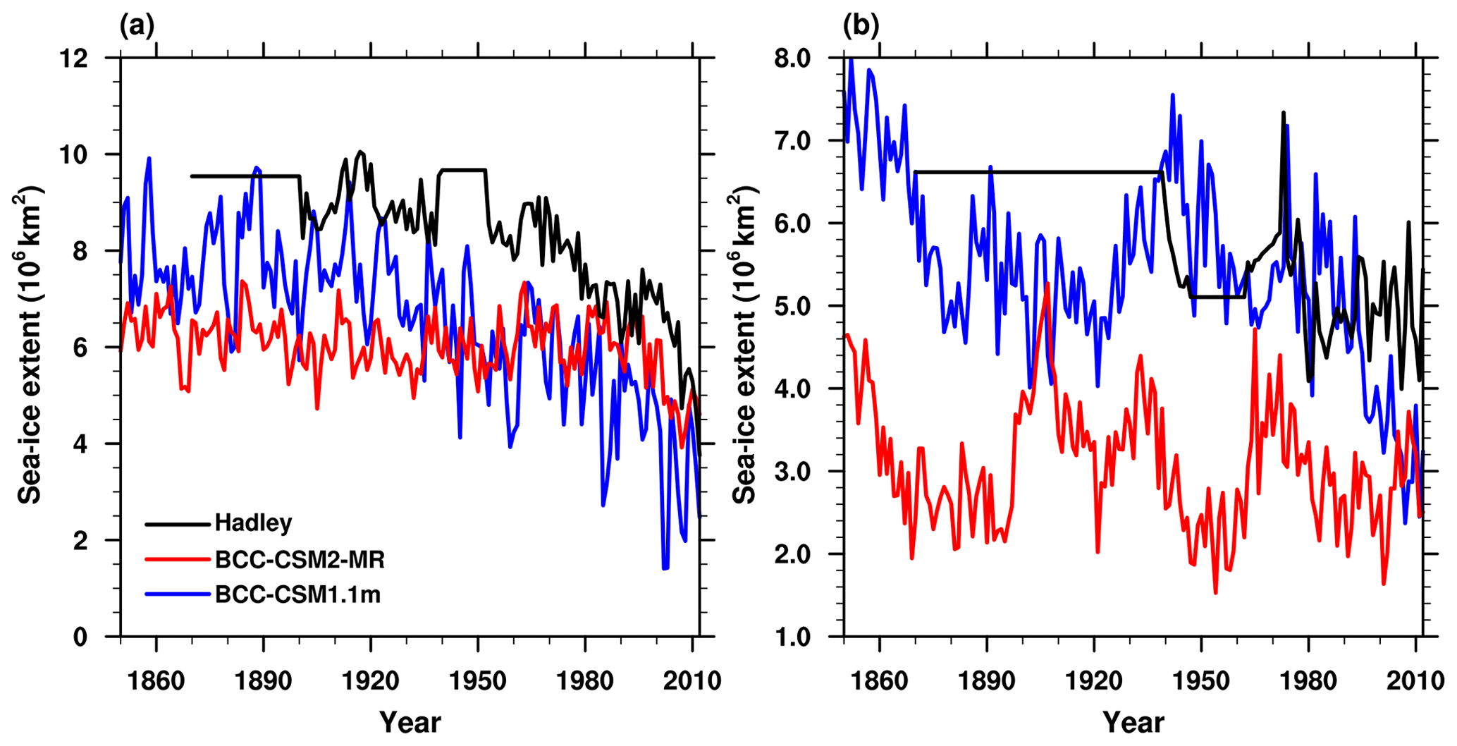
Figure 14Time series of the sea-ice extent from 1851 to 2012 for (a) the Arctic in September and (b) the Antarctic in March as simulated in BCC-CSM2-MR and BCC-CSM1.1m in addition to observations derived from the Hadley Centre Sea Ice and Sea Surface Temperature data set (Rayner et al., 2003).
Figure 15 shows the seasonal cycle of the sea-ice extent (SIE) and thickness averaged for the period from 1980 to 2005 in the two polar regions in our models. Observations of the sea-ice extent from the Hadley Centre data and sea-ice thickness from the ECMWF are also plotted for the purpose of comparison. Observations show that the Arctic sea-ice cover reaches a minimum extent of 6.9×10⁶ km2 in September and rises to a maximum extent of 16.0×10⁶ km2 in March (Fig. 15a). The two models can both capture the seasonal variation and pattern, but large biases in BCC-CSM1.1m exist in magnitude, especially in boreal winter, which are evidently improved in BCC-CSM2-MR. As for the Antarctic SIE (Fig. 15b), the ice cover in two models also undergos a very large seasonal cycle, which is similar to observations. However, SIE in BCC-CSM1.1m is too extensive throughout most of the year, particularly in Southern Hemisphere winter. Comparatively, the new model BCC-CSM2-MR simulates a relatively smaller seasonal cycle than that in BCC-CSM1.1 which is closer to the observations, except in February to March. In terms of ice thickness (Fig. 15c, d), the two models simulate a thinner ice cover compared with observations in all seasons for both the Arctic and Antarctic. The most remarkable improvements with respect to BCC-CSM2-MR appear in the Arctic in the boreal warm seasons, especially from June to September, with thicker ice presented in the Arctic Ocean. These improvements may be partly achieved due to the new model physics such as schemes for turbulent flux over sea ice and ocean surfaces, cloud fraction, or atmospheric circulation improvements at high latitudes. However, in the Antarctic, the ice thickness in BCC-CSM2-MR becomes worse and even much thinner than that in BCC-CSM1.1m in almost all year.
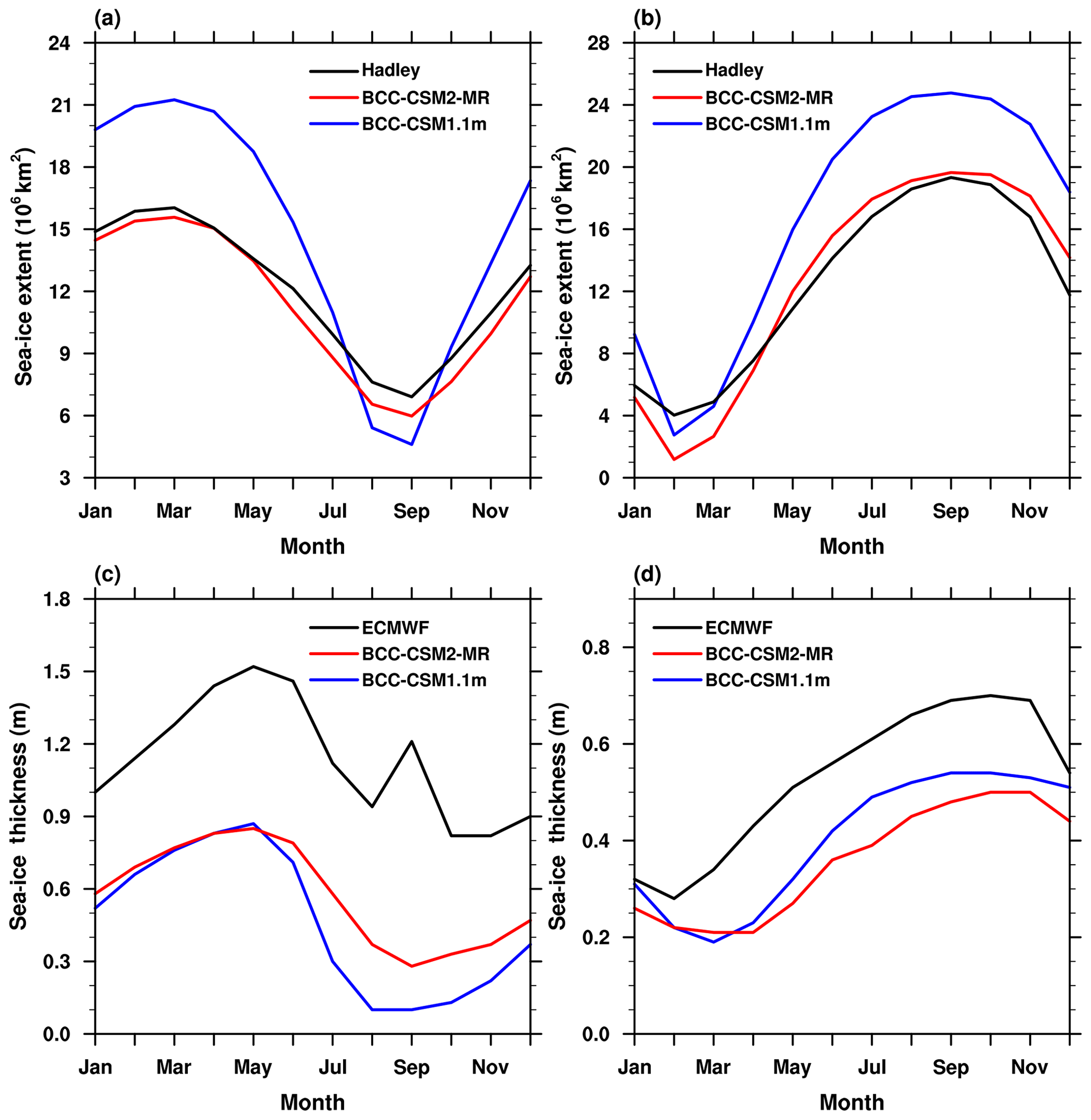
Figure 15The mean (1980–2005) seasonal cycle of sea-ice extent (a, b, the ocean area with a sea-ice concentration of at least 15 %) and mean thickness (c, d) in the Northern Hemisphere (a, c) and the Southern Hemisphere (b, d). The observed seasonal cycles of sea-ice extent in (a) and (b) are derived from the 1980 to 2005 Hadley Centre Sea Ice and Sea Surface Temperature data set (Rayner et al., 2003), and the ice thickness in (c, d) are derived from the 1980 to 2005 global gridded data set based on the European Center for Medium-Range Weather Forecast (Tietsche, et al., 2014).
The Atlantic Meridional Overturning Circulation (AMOC) plays a significant role in driving the global climate variation (Caesar et al., 2018). The AMOC consists of two primary overturning cells. In the upper cell, warm water flows northward in the upper 1000 m to supply the formation of the North Atlantic Deep Water (NADW), which returns southward in the depth range of approximately 1500 to 4000 m. In contrast, in the lower cell, the Antarctic Bottom Water (AABW) flows northward in the Atlantic basin beneath the NADW. Figure 16 shows the time-averaged AMOC simulated by the two coupled model versions. The two main cells are well depicted. The lower branch of the NADW is much deeper in BCC-CSM2-MR than in BCC-CSM1.1m, as indicated by the depth of the zero-contour line. Moreover, the central intensity of the NADW in BCC-CSM2-MR is over 22.5 Sv; this value is about 2.5 Sv stronger than that seen in BCC-CSM1.1m and is close to the observation-based value (25 Sv in Talley et al., 2013).
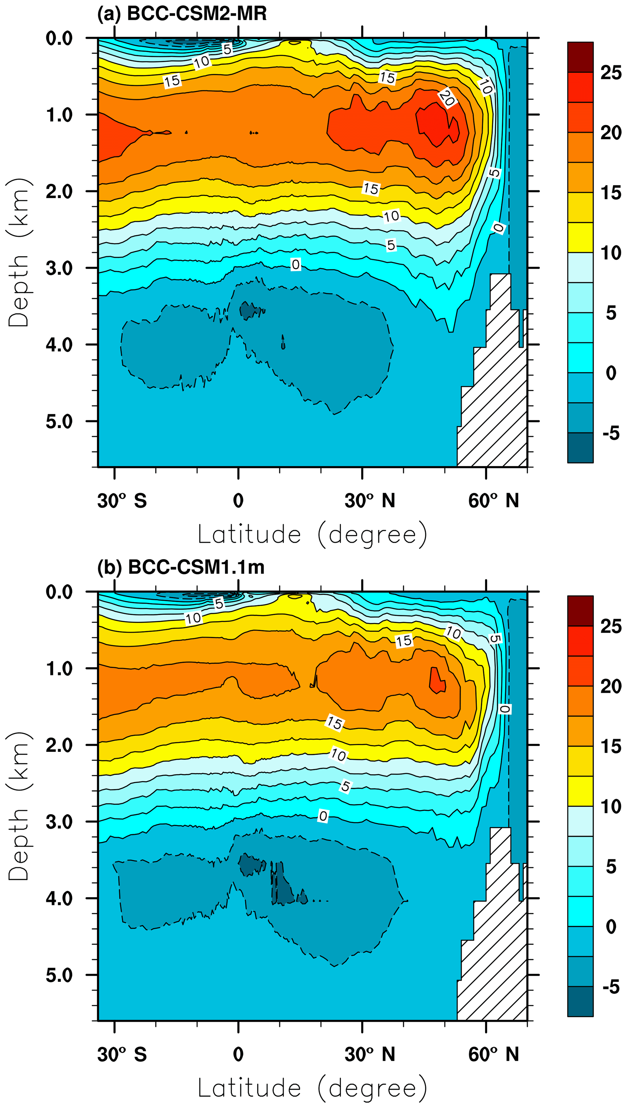
Figure 16Zonally averaged streamfunction of the Atlantic Meridional Overturning Circulation (AMOC) for the period from 1980 to 2005 in BCC-CSM2-MR (a) and BCC-CSM1.1m (b). (Units: Sv.)
4.7 Evaluation of models regarding their performance in East Asia
A good simulation of climate over East Asia is always a challenging issue for the climate modeling community, as the region is under the influences of complex topography (the high Tibetan Plateau) and atmospheric circulations from low latitudes (the tropical monsoon circulation) and from higher latitudes. Figure 17 plots a Taylor diagram to show the model performance of the main climate variables over East Asia covering the following region: 100–140∘ E, 20–50∘ N. Both BCC-CSM1.1m (blue figures) and BCC-CSM2-MR (red figures) are plotted for precipitation, sea level pressure, and atmospheric general circulation variables. There is a clear and remarkable improvement from CMIP5 to CMIP6 in the BCC models. The amelioration is seen in both the spatial pattern correlation (radial lines) and in the ratio of the standard deviations (circles from the origin).
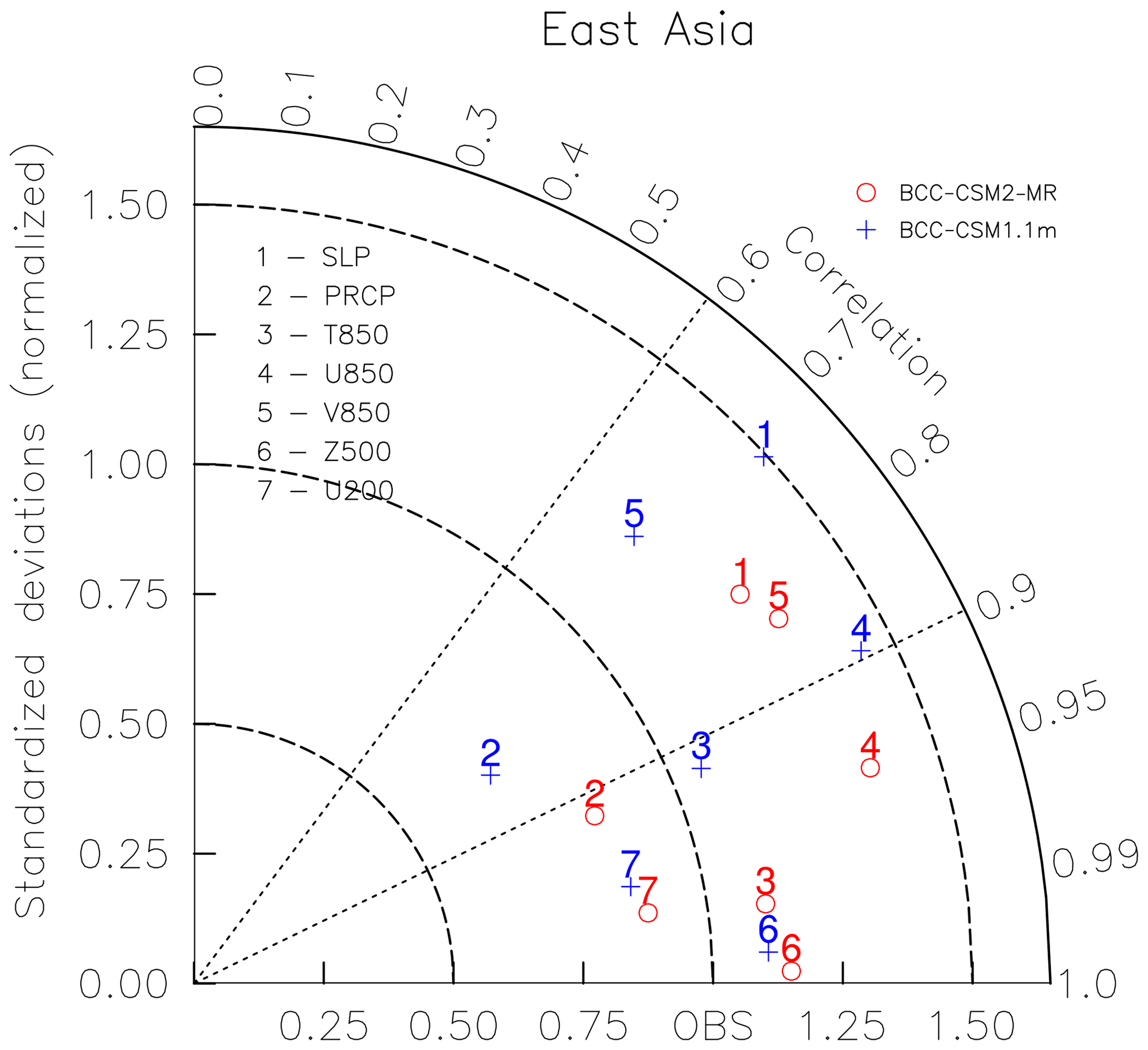
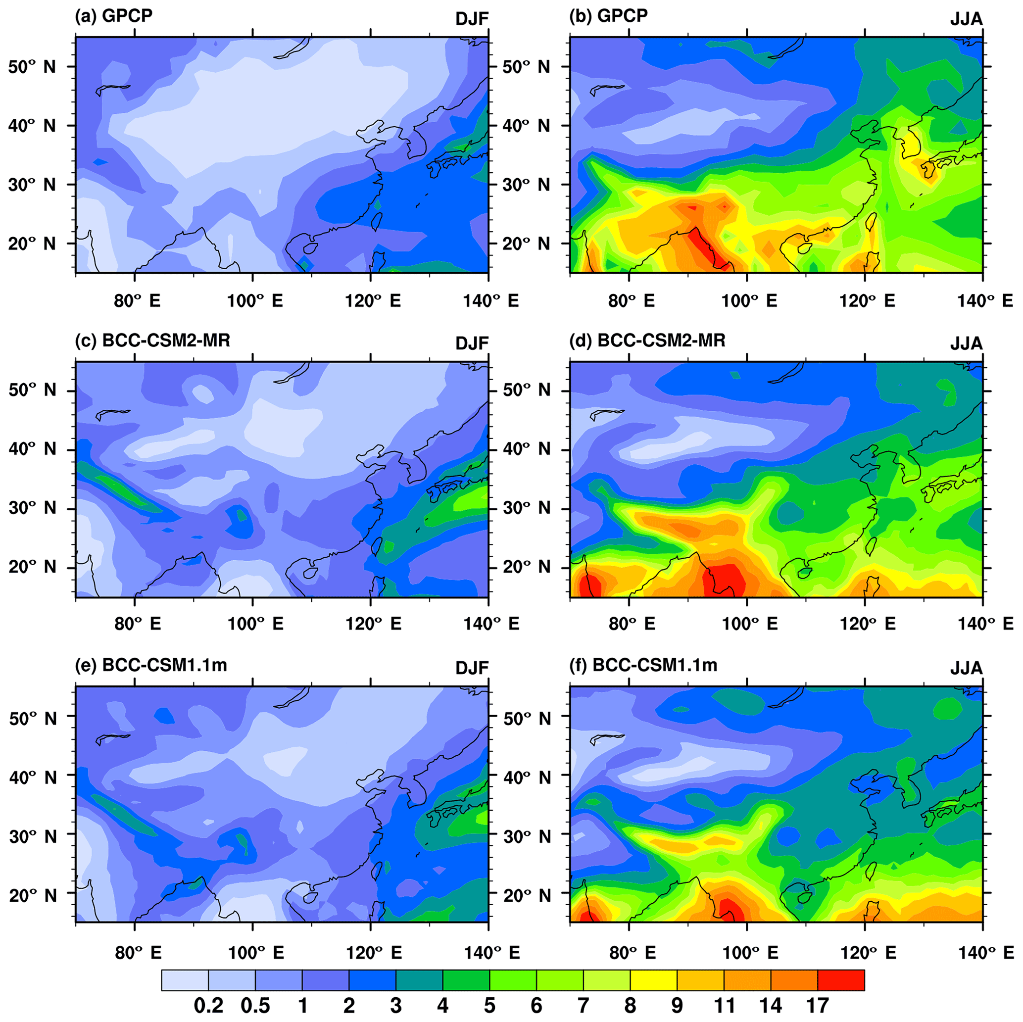
Figure 18Regional distribution maps of precipitation climatology (averaged from 1980 to 2005) for December–January–February (a, c, e) and June–July–August (b, d, f) from (a) GPCP, (b) BCC-CSM2-MR, and (c) BCC-CSM1.1m. (Units: mm day−1.)
Figure 18 shows the 1980–2005 climatology of December–January–February and June–July–August averaged precipitation over China and its surroundings. In boreal winter, GPCP precipitations show a rain belt from southeastern China to Japan and another rain belt along the southwestern flank of the Tibetan Plateau. In BCC-CSM1.1m the winter precipitation is too weak in southeastern China and too strong near Japan, compared with GPCP observations. This rain belt in BCC-CSM2-MR obviously spreads westward and is much closer to observations. However, the rain belt along the southwestern flank of the Tibetan Plateau in BCC-CSM2-MR becomes too strong. In boreal summer, large dry biases over eastern China are present in BCC-CSM1.1m. These biases are reduced in BCC-CSM2-MR. The center of precipitation around Japan is also well simulated in BCC-CSM2-MR.
The East Asian summer monsoon rainfall has a seasonal progression from south to north at the beginning of summer and then a quick retreat to the south when the summer monsoon terminates (as shown in Fig. 19a). This phenomenon is strongly related to the fact that the East Asian monsoon rainfall mainly takes place in the frontal zone between the warm and humid air mass from the south and cold and dry air mass from the north. This seasonal migration is also accompanied by a meridional movement of the Western North Pacific Subtropical High, an important atmospheric center of action controlling the climate of the region. In Fig. 19b and c, we compare the two models in terms of the seasonal migration of the monsoon rainfall. In the old model, rainfall was too weak. The new model produces more precipitation. In terms of seasonal match, both models show a delay of the peak rainfall by about 1 month, or even longer in BCC-CSM2-MR.
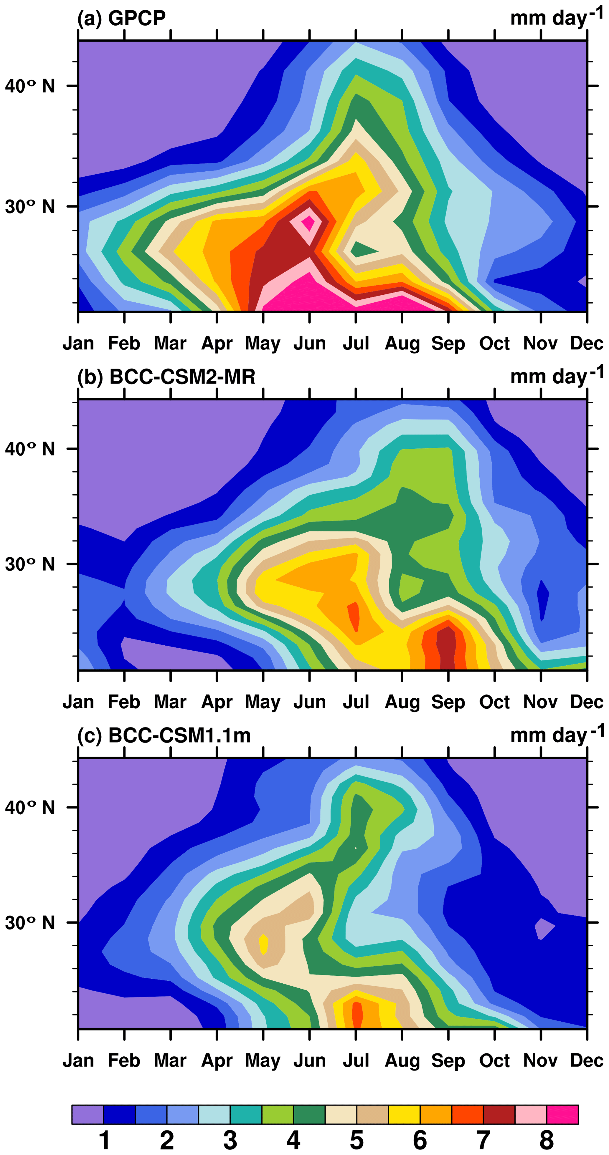
Figure 19Latitude (from 20 to 25∘ N) – month (January to December) diagrams showing variations of monthly precipitation averaged over 100–120∘ E and for the 1980–2005 period. (a) GPCP, (b) BCC-CSM2-MR, and (c) BCC-CSM1.1m. (Units: mm d−1.)
Figure 20Local times of the maximum frequency of rainfall occurrence in March–April–May (a, b, c), June–July–August (d, e, f), and September–October–November (g, h, i) over China and its surrounding areas for BCC-CSM2-MR (b, e, h), BCC-CSM1.1m (c, f, i), and TRMM data (a, d, g, Huffman et al., 2014). The rainfall occurrence is defined as hourly precipitation larger than 1 mm.
Finally, let us examine the rainfall diurnal cycle in summer. Figure 20 shows the timing of the rainfall diurnal cycle from observation and the two models. Main zones of nocturnal rainfall can be recognized on the south flank of the Tibetan Plateau, in the Sichuan Basin in the east of the Tibetan Plateau, and in the north of Xinjiang in central Asia. There is also a zone of nocturnal rainfall in the lower reach of the Yellow River, which is mainly under the influence of nocturnal rainfall in the Bohai Sea region. Other regions over land experience a diurnal rainfall peak in the afternoon after 16:00 LT. The diurnal cycle of rainfall was extensively studied in Jin et al. (2013) in terms of the physics causing the diurnal cycle; however, simulating the diurnal cycle well is always a major challenge for climate modeling. We can see that it is not very well simulated in our old model, and in East China the peak occurs from 00:00 to 04:00 LT. Nevertheless, the improvement is quite spectacular in our new model with the rainfall peak delayed in the afternoon. Such an improvement is due to the implementation of our new trigger scheme in convection parameterization.
This paper presents the main advancements of the BCC climate system models from CMIP5 to CMIP6 and focuses on the description of the CMIP6 version BCC-CSM2-MR and the CMIP5 version BCC-CSM1.1m, especially with respect to the model physics. Main updates to the model physics include a modification of the deep convection parameterization, a new scheme for the cloud fraction, indirect effects of aerosols through clouds and precipitation, and the gravity wave drag generated by deep convection. Surface processes in BCC-AVIM have also been significantly improved for the soil water freezing treatment, the snow aging effect on surface albedo, and the timing of vegetation leaf unfolding, growth, and withering. A four-stream radiation transfer within the vegetation canopy has replaced the two-stream radiation transfer. There is also a new treatment for rice paddy waters. Furthermore, new schemes for surface turbulent fluxes of momentum, heat, and water at the interface of atmosphere and sea/sea ice are used.
The evaluation of model performance in simulating present-day climatology is presented for main climate variables, such as surface air temperature, precipitation, and atmospheric circulation for the globe and for East Asia. Emphasis is put on the comparison between the CMIP5 and CMIP6 model versions (BCC-CSM2-MR versus BCC-CSM1.1m). The globally averaged TOA net energy budget is 0.85 W m−2 in BCC-CSM2-MR and 0.98 W m−2 in BCC-CSM1.1m. Both versions have a very good energy equilibrium. Model biases of excessive cloud shortwave and longwave radiative forcings over low latitudes in BCC-CSM1.1m are obviously reduced in BCC-CSM2-MR. When Taylor diagrams are used to compare the two models for spatial patterns of the main climate variables such as 2 m surface air temperature, precipitation, and atmospheric general circulation, BCC-CSM2-MR shows an overall improvement at both the global scale and the regional scale in East Asia. These improvements in BCC-CSM2-MR are believed to have been achieved due to the new scheme of cloud fraction and the consideration of indirect effects of aerosol on clouds and precipitation. The cold tongue bias of SST in the equatorial Pacific in BCC-CSM1.1m still exists in BCC-CSM2-MR. BCC-CSM1.1m has a severe bias with respect to the sea-ice extent (SIE) and thickness (Tan et al., 2015): it is too extensive in cold seasons and less extensive in warm seasons in both hemispheres. The most impressive improvements in BCC-CSM2-MR appear in the boreal warm seasons, especially from June to September, with thicker ice present in the Arctic Ocean. However, in the Southern Hemisphere, the sea-ice extent and thickness in BCC-CSM2-MR become even smaller than those in the previous model version. This is still an issue that needs to be addressed in our future work. There is another model bias of weak oceanic overturning circulation in BCC-CSM1.1m. This bias is reduced in the new version BCC-CSM2-MR, and the strength of the AMOC is increased.
Further evaluations are performed on climate variabilities at different timescales, including the long-term trend of global warming in the 20th century, the QBO, the MJO, and the diurnal cycle of precipitation. The globally averaged annual-mean surface air temperature from the historical simulation of BCC-CSM2-MR is much closer to the HadCRUT4 observations than BCC-CSM1.1m, and the observed global warming hiatus or warming slowdown in the period from 1998 to 2013 is captured in some realizations of BCC-CSM2-MR. With a higher vertical resolution and the inclusion of the gravity wave drag generated by deep convection, the new version BCC-CSM2-MR is able to reproduce the stratospheric QBO, whereas the QBO even does not exist in BCC-CSM1.1m. Further investigations on physical mechanisms controlling the QBO simulation in BCC-CSM2-MR will be reported in the future. The MJO is a very important atmospheric oscillation at intra-seasonal scales and main features are reproduced and improved in BCC-CSM2-MR, but with an intensity that is still weaker than its counterpart in the observations. At an interannual scale, the BCC-CSM1.1m shows overly strong variations of the Nino 3.4 SST index, but overly short and overly regular periodicity for ENSO. BCC-CSM2-MR shows a weaker amplitude for the Nino 3.4 SST index, which is an improvement and is closer to HadISST observations. The rainfall diurnal cycle in China has strong regional variations with pronounced nocturnal rainfalls in the Sichuan Basin and in northern China near the Bohai Sea and the coast. The diurnal rainfall generally peaks in the afternoon (local time) for most other land regions. BCC-CSM2-MR shows a clear improvement of the rainfall diurnal peaks compared with the CMIP5 model (BCC-CSM1.1m). This improvement of the rainfall diurnal variation is strongly related to the modification of the deep convection scheme.
Finally, we also evaluate the climate sensitivity to increasing CO2 in the standard simulation of 1 % CO2 increase per year (1pctCO2) and the 4× CO2 abrupt-change simulation. The transient climate response in the new CMIP6 model version BCC-CSM2-MR is lower than that seen in the previous CMIP5 model BCC-CSM1.1m, whereas the equilibrium climate sensitivity (ECS) for BCC-CSM2-MR is slightly higher than its counterpart in BCC-CSM1.1m.
From our model evaluations, we find that although basic features of the QBO can be simulated in BCC-CSM2-MR, the magnitude between the westerly and easterly interchange is still too weak. We also note that there are large biases of air temperature and winds in the stratosphere. Therefore, improvement of the stratospheric temperature and circulation simulations is an important priority in the future development of BCC models. In addition, the sea-ice simulation in the Antarctic region has large biases, which need to be improved.
Source codes of the BCC models are freely available upon request from Tongwen Wu (twwu@cma.gov.cn). Model output of the BCC models for both the CMIP5 and CMIP6 simulations described in this paper is distributed through the Earth System Grid Federation (ESGF) and is freely accessible via the ESGF data portals after registration. Details regarding ESGF are presented on the CMIP Panel website at http://www.wcrp-climate.org/index.php/wgcm-cmip/about-cmip (last access: 12 April 2019).
TW led the BCC-CSM development. TW and XX designed the experiments and carried them out. TW, LL, and XL wrote the final paper with contributions from all co-authors.
The authors declare that they have no conflict of interest.
This work was supported by The National Key Research and Development Program of China (grant no. 2016YFA0602100). Two anonymous reviewers are acknowledged for their constructive comments on earlier versions of the paper.
This paper was edited by Juan Antonio Añel and reviewed by two anonymous referees.
Adler, R. F. and Chang, A.: The Version 2 Global Precipitation Climatology Project (GPCP) Monthly Precipitation Analysis (1979–Present), J. Hydrometeorol., 4, 1147–1167, 2003.
Albrecht, B.: Aerosols, cloud microphysics, and fractional cloudiness, Science, 245, 1227–1230, 1989.
Alexander, M. J., May, P. T., and Beres, J. H.: Gravity waves generated by convection in the Darwin area during the Darwin Area Wave Experiment, J. Geophys. Res., 109, D20S04, https://doi.org/10.1029/2004JD004729, 2004.
Allen, M., Stott, P., Mitchell, J., Schnur, R., and Delworth, T.: Quantifying the uncertainty in forecasts of anthropogenic climate change, Nature, 407, 617–620, 2000.
Arora, V. K. and Boer, G. J.: A parameterization of leaf phenology for the terrestrial ecosystem component of climate models, Glob. Change Biol., 11, 39–59, https://doi.org/10.1111/j.1365-2486.2004.00890.x, 2005.
Andreas, E. L.: A theory for the scalar roughness and the scalar transfer coefficients over snow and sea ice, Bound.-Lay. Meteorol., 38, 159–184, 1987.
Andreas, E. L.: Parameterizing scalar transfer over snow and ice: A review, J. Hydrometeorol., 3, 417–432, 2002.
Andreas, E. L., Horst, T. W., Grachev, A. A., Persson, P. O. G., Fairall, C. W., and Guest, P. S., and Jordan, R. E.: Parametrizing turbulent exchange over summer sea ice and the marginal ice zone, Q. J. Roy. Meteor. Soc., 136, 927–943, 2010a.
Andreas, E. L., Persson, P. G., Jordan, R. E., Horst, T. W., Guest, T. S., Grachev, A. A., and Fairall, C. W.: Parameterizing turbulent exchange over sea ice in winter, J. Hydrometeorol., 11, 87–104, 2010b.
Andrews, T., Gregory, J. M., Webb, M. J., and, Taylor, K. E.: Forcing, feedbacks and climate sensitivity in CMIP5 coupled atmosphere-ocean climate models, Geophys. Res. Lett, 38, L09712, https://doi.org/10.1029/2012GL051607, 2012.
Beres, J. H., Alexander, M. J., and Holton, J. R.: A method of specifying the gravity wave spectrum above convection based on latent heating properties and background wind, J. Atmos. Sci., 61, 324–337, 2004.
Boucher, O. and Lohmann, U.: The sulphate-CCN-cloud albedo effect – a sensitivity study with two general circulation models, Tellus B, 47, 281–300, 1995.
Caesar, L., Rahmstorf, S., Robinson, A., Feulner, G., and Saba, V.: Observed fingerprint of a weakening Atlantic Ocean overturning circulation, Nature, 556, 191–196, 2018.
Campin, J. M. and Goosse, H.: Parameterization of density-driven downsloping flow for a coarse-resolution ocean model in z-coordinate, Tellus A, 51, 412–430, 1999.
Cao, M. and Woodward, F. I.: Net primary and ecosystem production and carbon stocks of terrestrial ecosystems and their responses to climate change, Glob. Change Biol., 4, 185–198, 1998.
Chen, A., Li, W. P., Li, W. J., and Liu, X.: An observational study of snow aging and the seasonal variation of snow albedo by using data from Col de Porte, France, Chinese Sci. Bull., 59, 4881–4889, 2014.
Chen, C. and Cotton, W. R.: The physics of the marine stratocumulus-capped mixed layer, J. Atmos. Sci., 44, 2951–2977, 1987.
Collins, W. D., Rasch, P. J., Boville, B. A., Hack, J. J., McCaa, J. R., Williamson, D. L., Kiehl, J. T., Briegleb, B., Bitz C., Lin, S. J., Zhang, M. H., and Dai, Y. J.: Description of the NCAR community atmosphere model (CAM3), National Center for Atmospheric Research, Boulder, Colorado, Technical Report NCAR/TN-464 + STR, 226 pp, 2004.
Collins, W. J., Lamarque, J.-F., Schulz, M., Boucher, O., Eyring, V., Hegglin, M. I., Maycock, A., Myhre, G., Prather, M., Shindell, D., and Smith, S. J.: AerChemMIP: quantifying the effects of chemistry and aerosols in CMIP6, Geosci. Model Dev., 10, 585–607, https://doi.org/10.5194/gmd-10-585-2017, 2017.
Danabasoglu, G., Yeager, S. G., Bailey, D., Behrens, E., Bentsen, M., Bi, D., Biastoch, A., Böning, C., Bozec, A., Canuto, V. M., Cassou, C., Chassignet, E., Coward, A. C., Danilov, S., Diansky, N., Drange, H., Farneti, R., Fernandez, E., Fogli, P. G., Forget, G., Fujii, Y., Griffies, S. M., Gusev, A., Heimbach, P., Howard, A., Jung, T., Kelley, M., Large, W. G., Leboissetier, A., Lu, J., Madec, G., Marsland, S. J., Masina, S., Navarra, A., Nurser, A. J. G., Pirani, A., Salas y Mélia, D., Samuels, B. L., Scheinert, M., Sidorenko, D., Treguier, A.-M., Tsujino, H., Uotila, P., Valcke, S., Voldoire, A., and Wang, Q.: North Atlantic simulations in Coordinated Ocean-ice Reference Experiments phase II (CORE-II). Part I: Mean States, Ocean Model., 73, 76–107, https://doi.org/10.1016/j.ocemod.2013.10.005, 2014.
Dee, D. P., Uppala, S. M., Simmons, A. J., Berrisford, P., Poli, P., Kobayashi, S., Andrae, U., Balmaseda, M. A., Balsamo, G., Bauer, P., Bechtold, P., Beljaars, A. C. M., Berg L., Bidlot, J., Bormann, N., Delsol, C., Dragani, R., Fuentes, M., Geer, A. J., Haimberger, L., Healy, S. B., Hersbach, H., Holm, E. V., Isaksen, L., Kallberg, P., Kohler, M., Matricardi, M., NcNally, A. P., Monge-Sanz, B. M., Morcrette, J.-J., Park, B.-K., Peubey, C., Rosnay, P., Tavolato, C., Thepaut, J.-N., and Vitart F.: The ERA-Interim reanalysis: configuration and performance of the data assimilation system, Q. J. R. Meteor. Soc., 137, 553–597, https://doi.org/10.1002/qj.828, 2011.
Ding, Y. H., Liu, Y. M., Song, Y. J., and Li, Q. Q.: Research and experiments of the dynamical model system for short-term climate prediction, Climatic and Environmental Research, 7, 236–246, 2002 (in Chinese).
Eyring, V., Bony, S., Meehl, G. A., Senior, C. A., Stevens, B., Stouffer, R. J., and Taylor, K. E.: Overview of the Coupled Model Intercomparison Project Phase 6 (CMIP6) experimental design and organization, Geosci. Model Dev., 9, 1937–1958, https://doi.org/10.5194/gmd-9-1937-2016, 2016.
Fyfe, J. C., Meehl, G. A., England, M. H., Mann, M. E., Santer, B. D., Flato, G. M., Hawkins, E., Gillett, N. P., Xie, S.-P., Kosaka, Y., and Swart, N. C.: Making sense of the early-2000s warming slowdown, Nat. Clim. Change, 6, 224–228, 2016.
Gent, P. R. and Mcwilliams, J. C.: Isopycnal mixing in ocean circulation Models, J. Phys. Oceanogr., 20, 150–155, 1990.
Gregory, J. M., Ingram, W. J., Palmer, M. A., Jones, G. S., Stott, P. A., Thorpe, R. B., Lowe, J. A., Johns, T. C., and Williams, K. D.: A new method for diagnosing radiative forcing and climate sensitivity, Geophys. Res. Lett., 31, L03205, https://doi.org/10.1029/2003GL018747, 2004.
Gregory, J. M., Webb, M. J., and Taylor, K. E.: Forcing, feedbacks and climate sensitivity in CMIP5 coupled atmosphere-ocean climate models, Geophys. Res. Lett., 39, L09712, https://doi.org/10.1029/2012GL051607, 2012.
Griffies, S. M., Gnanadesikan, A., Dixon, K. W., Dunne, J. P., Gerdes, R., Harrison, M. J., Rosati, A., Russell, J. L., Samuels, B. L., Spelman, M. J., Winton, M., and Zhang, R.: Formulation of an ocean model for global climate simulations, Ocean Sci., 1, 45–79, https://doi.org/10.5194/os-1-45-2005, 2005.
Guenther, A. B., Jiang, X., Heald, C. L., Sakulyanontvittaya, T., Duhl, T., Emmons, L. K., and Wang, X.: The Model of Emissions of Gases and Aerosols from Nature version 2.1 (MEGAN2.1): an extended and updated framework for modeling biogenic emissions, Geosci. Model Dev., 5, 1471–1492, https://doi.org/10.5194/gmd-5-1471-2012, 2012.
Haarsma, R. J., Roberts, M. J., Vidale, P. L., Senior, C. A., Bellucci, A., Bao, Q., Chang, P., Corti, S., Fuckar, N. S., Guemas, V., von Hardenberg, J., Hazeleger, W., Kodama, C., Koenigk, T., Leung, L. R., Lu, J., Luo, J.-J., Mao, J., Mizielinski, M. S., Mizuta, R., Nobre, P., Satoh, M., Scoccimarro, E., Semmler, T., Small, J., and von Storch, J.-S.: High Resolution Model Intercomparison Project (HighResMIP v1.0) for CMIP6, Geosci. Model Dev., 9, 4185–4208, https://doi.org/10.5194/gmd-9-4185-2016, 2016.
Hack, J. J.: Parameterization of moist convection in the National Center for Atmospheric Research Community Climate Model (CCM2), J. Geophys. Res., 99, 5551–5568, 1994.
Holtslag, A. A. M. and Boville, B. A.: Local versus nonlocal boundary-layer diffusion in a global climate model, J. Climate, 6, 1825–1842, 1993.
Huffman, G., Bolvin, D., Braithwaite, D., Hsu, K., Joyce, R., and Xie, P.: Integrated Multi-satellitE Retrievals for GPM (IMERG), version 4.4, NASA's Precipitation Processing Center, available at: ftp://arthurhou.pps.eosdis.nasa.gov/gpmdata/ (last access: 31 March 2015), 2014.
IPCC: Climate Change 2013: The Physical Science Basis, edited by: Stocker, T. F., Qin, D., Plattner, G.-K., Tignor, M., Allen, S. K., Boschung, J., Nauels, A., Xia, Y., Bex V., and Midgley, P. M., Cambridge University Press, Cambridge, United Kingdom and New York, NY, USA, 2013.
Ji, J.: A climate-vegetation interaction model: Simulating physical and biological processes at the surface, J. Biogeogr., 22, 2063–2069, 1995.
Ji, J., Huang, M., and Li, K.: Prediction of carbon exchange between China terrestrial ecosystem and atmosphere in 21st century, Sci. China Ser. D, 51, 885–898, 2008.
Jiang, X., Waliser, D. E., Xavier, P. K., Petch, J., Klingaman, N. P., Woolnough, S. J., Guan, B., Bellon, G., Crueger, T., DeMott, C., Hannay, C., Lin, H., Hu, W., Kim, D., Lappen, C., Lu, M.–M., Ma, H.-Y., Miyakawa, T., Ridout, J. A., Schubert, S. D., Scinocca, J., Seo, K.-H., Shindo, E., Song, X., Stan, C., Tseng, W.-L., Wang, W., Wu, T., Wyser, K., Wu, X., Zhang, G. J., and Zhu, H.: Vertical structure and physical processes of the Madden-Julian oscillation: Exploring key model physics in climate simulations, J. Geophys. Res.-Atmos., 120, 4718–4748, https://doi.org/10.1002/2014JD022375, 2015.
Jin, X., Wu, T., and Li, L.: The quasi-stationary feature of nocturnal precipitation in the Sichuan Basin and the role of the Tibetan Plateau, Clim. Dynam., 41, 977–994, https://doi.org/10.1007/s00382-012-1521-y, 2013.
Jones, C. D., Arora, V., Friedlingstein, P., Bopp, L., Brovkin, V., Dunne, J., Graven, H., Hoffman, F., Ilyina, T., John, J. G., Jung, M., Kawamiya, M., Koven, C., Pongratz, J., Raddatz, T., Randerson, J. T., and Zaehle, S.: C4MIP – The Coupled Climate–Carbon Cycle Model Intercomparison Project: experimental protocol for CMIP6, Geosci. Model Dev., 9, 2853–2880, https://doi.org/10.5194/gmd-9-2853-2016, 2016.
Klein, S. A. and Hartmann, D. L.: The seasonal cycle of low stratiform clouds, J. Climate, 6, 1587–1606, 1993.
Kristjánsson, J. E., Edwards, J. M., and Mitchell, D. L.: Impact of a new scheme for optical properties of ice crystals on climates of two GCMs, J. Geophys. Res., 105, 10063–10079, https://doi.org/10.1029/2000JD900015, 2000.
Lamarque, J.-F., Emmons, L. K., Hess, P. G., Kinnison, D. E., Tilmes, S., Vitt, F., Heald, C. L., Holland, E. A., Lauritzen, P. H., Neu, J., Orlando, J. J., Rasch, P. J., and Tyndall, G. K.: CAM-chem: description and evaluation of interactive atmospheric chemistry in the Community Earth System Model, Geosci. Model Dev., 5, 369–411, https://doi.org/10.5194/gmd-5-369-2012, 2012.
Large, W. G., McWilliams, J. C., and Doney, S. C.: Oceanic vertical mixing: A review and a model with a nonlocal boundary layer parameterization, Rev. Geophys., 32, 363–403, 1994.
Li, J. D., Wang, W.-C., Liao, H., and Chang, W. Y.: Past and future direct radiative forcing of nitrate aerosol in East Asia, Theor. Appl. Climatol., 121, 445–458, 2015.
Liou, K. N.: An Introduction to Atmospheric Radiation, China Meteorological Press, Beijing, China, 313–327, 2004 (in Chinese).
Liu, Y. and Daum, P. H.: Indirect warming effect from dispersion forcing, Nature, 419, 580–581, 2002.
Loeb, N. G., Lyman, J. M., Johnson, G. C,, Allan, R. P., Doelling, D. R., Wong, T., Soden, B. J., and Stephens, G. L.: Observed changes in top-of-the-atmosphere radiation and upper-ocean heating consistent within uncertainty, Nat. Geosci., 5, 110–113, https://doi.org/10.1038/ngeo1375, 2012.
Lu, B. and Ren, H.-L.: Improving ENSO periodicity simulation by adjusting cumulus entrainment in BCC_CSMs, Dynam. Atmos. Oceans, 76, 127–140, 2016.
Lu, Y., Zhou, M., and Wu, T.: Validation of parameterizations for the surface turbulent fluxes over sea ice with CHINARE 2010 and SHEBA data, Polar Res., 32, 20818, https://doi.org/10.3402/polar.v32i0.20818, 2013.
Martin, G.M., Johnson, D.W., and Spice, A.: The measurement and parameterisation of effective radius of droplets in warm stratocumulus clouds, J. Atmos. Sci., 51, 1823–1842, 1994.
McFarlane, N. A.: The effect of orographically excited gravity wave drag on the general circulation of the lower stratosphere and troposphere, J. Atmos. Sci., 44, 1775–1800, 1987.
Medhaug, I., Martin, B. S., Erich, M. F., and Knutti, R.: Reconciling controversies about the 'global warming hiatus', Nature, 545, 41–47, 2017.
Meehl, G. A., Boer, G. J., Covey, C., Latif, M., and Stouffer, R. J.: Intercomparison makes for a better climate model, Eos T. Am. Geophys. Un., 78, 445–451, https://doi.org/10.1029/97EO00276, 1997.
Morice, C, P., Kennedy, J. J., Rayner, N.A., and Jones, P.D.: Quantifying uncertainties in global and regional temperature change using an ensemble of observational estimates: The HadCRUT4 data set, J. Geophys. Res. 117, D08101, 2012.
Oleson, K. W., Lawrence, D. M., and Dai, Y. J.: Technical description of the Community Land Model (CLM), NCAR Technical Note NCAR/TN-461+STR, 173 pp., https://doi.org/10.5065/D6N877R0, 2004.
Peng, Y. and Lohmann, U.: Sensitivity study of the spectral dispersion of the cloud droplet size distribution on the indirect aerosol effect, Geophys. Res. Lett., 30, 1507, https://doi.org/10.1029/2003GL017192, 2003.
Pontikis, C. A. and Hicks, E.; Contribution to the cloud droplet effective radius parameterization, Geophys. Res. Lett. 19, 2227–2230, 1992.
Quaas, J., Boucher, O., and Lohmann, U.: Constraining the total aerosol indirect effect in the LMDZ and ECHAM4 GCMs using MODIS satellite data, Atmos. Chem. Phys., 6, 947–955, https://doi.org/10.5194/acp-6-947-2006, 2006.
Rahmstorf, S.: A fast and complete convection scheme for ocean models, Ocean Model., 101, 9–11, 1993.
Rasch, P. J. and Kristjánsson, J. E.: A comparison of the CCM3 model climate using diagnosed and predicted condensate parameterizations, J. Climate, 11, 1587–1614, 1998.
Rayner, N. A., Parker, D. E., Horton, E. B., Folland, C., Alexander, L., Rowell, D., Kent, E., and Kaplan, A.: Global analyses of sea surface temperature, sea ice, and night marine air temperature since the late nineteenth century, J. Geophys. Res., 108, 4407, https://doi.org/10.1029/2002JD002670, 2003.
Richter, J. H., Sassi, F., and Garcia, R. R.: Toward a physically based gravity wave source parameterization in a general circulation model, J. Atmos. Sci., 67, 136–156, 2010.
Stevens, B., Fiedler, S., Kinne, S., Peters, K., Rast, S., Müsse, J., Smith, S. J., and Mauritsen, T.: MACv2-SP: a parameterization of anthropogenic aerosol optical properties and an associated Twomey effect for use in CMIP6, Geosci. Model Dev., 10, 433–452, https://doi.org/10.5194/gmd-10-433-2017, 2017.
Sweeney, C., Gnanadesikan, A., Griffies, S. M., Harrison, M., Rosati, A., and Samuels, B.: Impacts of shortwave penetration depth on large-scale ocean circulation and heat transport, J. Phys. Oceanogr., 35, 1103–1119, 2005.
Talley, L. D.: Closure of the global overturning circulation through the Indian, Pacific, and Southern Oceans: Schematics and transports, Oceanography, 26, 80–97, 2013.
Tan, H. H., Zhang, L. J., Chu, M., Wu, T. W., Qiu, B., and Li, J. L.: An analysis of simulated global sea ice extent, thickness, and causes of error with the BCC_CSM model, Chinese Journal of Atmospheric Sciences, 39, 197–209, 2015 (in Chinese).
Taylor, K. E., Stouffer, R. J., and Meehl, G. A.: An Overview of Cmip5 and the Experiment Design, B. Am. Meteorol. Soc., 93, 485–498, 2012.
Tietsche, S., Balmaseda, M., Zuo, H., and Mogensen, K.: Arctic sea ice in the ECMWF MyOcean2 ocean reanalysis ORAP5, European Center for Medium-Range Weather Forecasts, Reading, UK, ECMWF Technical Memorandum No. 737, 33 pp., 2014.
Wielicki, B. A., Barkstrom, B. R., Harrison, E. F., Lee, R. B., Smith, G. L., and Cooper, J. E.: Clouds and the earth's radiant energy system (CERES): an earth observing system experiment, B. Am. Meteorol. Soc., 77, 853–868, 1996.
Winton, M.: A reformulated three-layer sea ice model, J. Atmos. Ocean. Tech., 17, 525–531, 2000.
Wu, T.: A Mass-Flux Cumulus Parameterization Scheme for Large-scale Models: Description and Test with Observations, Clim. Dynam., 38, 725–744, https://doi.org/10.1007/s00382-011-0995-3, 2012.
Wu, T. and Wu, G.: An empirical formula to compute snow cover fraction in GCMs, Adv. Atmos. Sci., 21, 529–535, 2004.
Wu, T., Yu, R., Zhang, F., Wang, Z., Dong, M., Wang, L., Jin, X., Chen, D. L., and Li, L.: The Beijing Climate Center atmospheric general circulation model: description and its performance for the present-day climate, Clim. Dynam., 34, 123–147, https://doi.org/10.1007/s00382-008-0487-2, 2010.
Wu, T., Yu, R., and Zhang, F.: A modified dynamic framework for atmospheric spectral model and its application, J. Atmos. Sci., 65, 2235–2253, 2008.
Wu, T., Li, W., Ji, J., Xin, X., Li, L., Wang, Z., Zhang, Y., Li, J., Zhang, F., Wei, M., Shi, X., Wu, F., Zhang, L., Chu, M., Jie, W., Liu, Y.,Wang, F., Liu, X., Li, Q., Dong, M., Liang, X., Gao, Y., and Zhang, J.: Global carbon budgets simulated by the Beijing climate center climate system model for the last century, J. Geophys. Res.-Atmos., 118, 4326–4347, https://doi.org/10.1002/jgrd.50320, 2013.
Wu, T., Song, L., Li, W., Wang, Z., Zhang, H., Xin, X., Zhang, Y., Zhang, L., Li, J., Wu, F., Liu, Y., Zhang, F., Shi, X., Chu, M., Zhang, J., Fang, Y., Wang, F., Lu,Y., Liu, X., Wei, M., Liu, Q., Zhou, W., Dong, M., Zhao, Q., Ji, J., Li, L., and Zhou, M.: An overview of BCC climate system model development and application for climate change studies, J. Meteorol. Res.-PRC, 28, 34–56, 2014.
Xia, K., Luo, Y., and Li, W. P.: Simulation of freezing and melting of soil on the northeast Tibetan Plateau, Chinese Sci. Bull., 56, 1–4, https://doi.org/10.1007/s11434-011-4542-8, 2011.
Xin, X., Wu, T., and Zhang, J.: Introduction of CMIP5 experiments carried out with the climate system models of Beijing Climate Center, Advances in Climate Change Research, 4, 41–49, https://doi.org/10.3724/SP.J.1248.2013.041, 2013.
Xu, L. and Penner, J. E.: Global simulations of nitrate and ammonium aerosols and their radiative effects, Atmos. Chem. Phys., 12, 9479–9504, https://doi.org/10.5194/acp-12-9479-2012, 2012.
Xu, K. M. and Krueger, S. K.: Evaluation of cloudiness parameterizations using a cumulus ensemble model, Mon. Weather Rev., 119, 342–367, 1991.
Zeng, X., Zhao, M., and Dickinson, R. E.: Intercomparison of bulk aerodynamic algorithms for the computation of sea surface fluxes using TOGA COARE and TAO data, J. Climate, 11, 2628–2644, 1998.
Zeng, X., Zhang, Q., Johnson, D., and Tao, W.-K.: Parameterization of wind gustiness for the computation of ocean surface fluxes at different spatial scales, Mon. Weather Rev., 130, 2125–2133, 2002.
Zhang, G. J.: Convective quasi-equilibrium in midlatitude continental environment and its effect on convective parameterization, J. Geophys. Res., 107, ACL 12-1–ACL 12-16, https://doi.org/10.1029/2001JD001005, 2002.
Zhang, M., Lin, W., Bretherton, C. S., Hack, J. J., and Rasch, P. J.: A modified formulation of fractional stratiform condensation rate in the NCAR community atmospheric model (CAM2), J. Geophys. Res., 108, 4035, https://doi.org/10.1029/2002JD002523, 2003.
Zhang, Y., Gao, Z., Li, D., Li, Y., Zhang, N., Zhao, X., and Chen, J.: On the computation of planetary boundary-layer height using the bulk Richardson number method, Geosci. Model Dev., 7, 2599–2611, https://doi.org/10.5194/gmd-7-2599-2014, 2014.
Zhou, W. Y., Luo, Y., Li, W. P., Shi, X. L., and Zhang, Y.: Comparative studies of different radiation schemes within vegetation in land model, Chinese Sci. Bull., 63, 2772–2784, https://doi.org/10.1360/N972018-00398, 2018.
- Abstract
- Introduction
- Transition of the BCC climate system model from CMIP5 to CMIP6
- Experimental design
- Evaluation and comparison between BCC CMIP5 and CMIP6 models
- Conclusions and discussion
- Code and data availability
- Author contributions
- Competing interests
- Acknowledgements
- Review statement
- References