libcloudph++ 2.0: aqueous-phase chemistry extension of the particle-based cloud microphysics scheme

This paper introduces a new scheme available in the library of algorithms for representing cloud microphysics in numerical models named libcloudph++. The scheme extends the particle-based microphysics scheme with a Monte Carlo coalescence available in libcloudph++ to the aqueous-phase chemical processes occurring within cloud droplets. The representation of chemical processes focuses on the aqueous-phase oxidation of the dissolved SO₂ by O₃ and H₂O₂. The particle-based microphysics and chemistry scheme allows for tracking of the changes in the cloud condensation nuclei (CCN) distribution caused by both collisions between cloud droplets and aqueous-phase oxidation.

The scheme is implemented in C++ and equipped with bindings to Python. The scheme can be used on either a CPU or a GPU, and is distributed under the GPLv3 license. Here, the particle-based microphysics and chemistry scheme is tested in a simple 0-dimensional adiabatic parcel model and then used in a 2-dimensional prescribed flow framework. The results are discussed with a focus on changes to the CCN sizes and comparison with other model simulations discussed in the literature.

1 Introduction

libcloudph++ is an open-source library of schemes for representing cloud microphysics in numerical models. It was first introduced in Arabas et al. (2015) where the authors present the different microphysics schemes available in the library, show its programming interface, and discuss its performance. The flagship component of libcloudph++ is the particle-based (i.e. particle tracking or “Lagrangian-in-droplet-radius-and-space”) microphysics scheme. The scheme resolves the evolution of the aerosol, cloud droplet, and rain drop¹ size spectrum. It allows for representing cloud microphysical processes from first principles and is especially well suited to track changes in the CCN size distribution that are caused by clouds (i.e. cloud-aerosol processing). The scheme can be used in models of any dimensionality or dynamical core, and can be run on both CPU and GPU. The main software design principle employed while developing libcloudph++ core code is the separation of concerns. The code is open-source and its programming interface is documented in Arabas et al. (2015). All those features facilitate further development and usage of libcloudph++.

Sulfate aerosols cool Earth's climate by scattering sunlight – and thus increasing Earth's shortwave albedo (direct radiative forcing) – and also by changing radiative properties of clouds (cloud albedo effect). According to chapter 8 of IPCC² Assessment Report (Myhre et al., 2013), the range of effective radiative forcings for all aerosol–radiation interactions is −0.95 to 0.05 W m⁻² and for aerosol–cloud interactions is −1.2 to 0.0 W m⁻². The level of scientific understanding in that report for the cloud albedo effect is still marked as “low”. From the air quality perspective, sulfur chemistry may lead to the creation of acid rain or acid fog in extreme cases (Dianwu et al., 1988; Wang et al., 2016). Based on analyses of 20 modelling studies, the review by Faloona (2009) marks wet deposition of aerosol sulfate, dry deposition of SO₂, and heterogeneous (aqueous phase) oxidation of SO₂ in aerosol particles and clouds as the most challenging to quantify in models. For an overview of the representation of sulfur oxidation in regional and global models see Ervens (2015). Aqueous-phase oxidation is reported as a dominant mechanism of the production of sulfate: a numerical study by Barth et al. (2000) reports that for the in-cloud conditions, aqueous-phase reactions account for 81 % of the sulfate production rate. According to their study, a total of ∼50 %–60 % of sulfate burden in the troposphere is produced by aqueous-phase chemistry. The gas-phase SO₂ is oxidized in a matter of days by gas-phase reactions, or within minutes or a few hours within clouds by aqueous-phase reactions, see the review by Faloona (2009).

From the cloud microphysics stand point, aqueous-phase oxidation of sulfur is interesting because it affects the CCN within water drops. Note that sulfate is a common component of aerosol particles (Zhang et al., 2007). The aqueous-phase oxidation of sulfur is irreversible, meaning that the produced sulfate remains within water drops and increases the dissolved CCN mass. Collisions and the subsequent coalescence of water drops as well as collisions between aerosol particles and water drops are another in-cloud irreversible process that affects aerosol particles. As water drops collide and coalesce, the newly created water drop carries the combined CCN mass of all of its colliding predecessors. Efficient collisions between cloud droplets may quickly lead to the onset of precipitation, which can in turn effectively cleanse the atmosphere from aerosol particles and water-soluble trace gases. In non-precipitating clouds, aerosol particles that served as CCN are altered by cloud microphysical and chemical processes and then return to the atmosphere after water drops evaporate (the process is referred to as the CCN deactivation, aerosol regeneration, aerosol recycling, or aerosol resuspension). The cloud-processed aerosol particles can be observed in measurements (Hoppel et al., 1986, 1994; Hudson et al., 2015; Werner et al., 2014). The case without precipitation reaching the surface is especially interesting as it allows for aerosol–cloud interactions to loop for several cloud life- cycles without removing the altered aerosol particles. The cloud-processed aerosol particles may again serve as CCN and influence microphysical properties of the next generation of clouds. The study of Pruppacher and Jaenicke (1995) estimates that on global average an atmospheric aerosol particle has been cycled 3 times by cloud systems. The particle-based microphysics and chemistry (PBMC) scheme introduced here offers a chance to represent the effects of such cloud-processing on CCN sizes stemming from both collisions between water drops and aqueous-phase oxidation reactions within water drops. The PBMC can be used in multidimensional simulations with a fully coupled dynamics model, which has not been possible before. To the authors knowledge, the presented scheme is the first to represent the impact of both collisions and aqueous-phase chemistry on the aerosol size spectrum in the particle-based microphysics framework.

This paper documents the extension of the particle-based microphysics scheme with a numerical scheme that represents aqueous-phase chemical reactions inside cloud droplets and the uptake of the trace gases into cloud droplets. The representation of chemical reactions includes only the aqueous-phase processes (i.e. no gas-phase chemical reactions) and revolves around oxidation of sulfur dissolved in water drops to sulfate. Two reaction paths are considered – the oxidation by ozone and by hydrogen peroxide. In total, six trace gases are included in the chemistry description: sulfur dioxide (SO₂), ozone (O₃), hydrogen peroxide (H₂O₂), carbon dioxide (CO₂), nitric acid (HNO₃), and ammonia (NH₃). Their dissolution and, if applicable, dissociation is resolved. The structure of the presented work is as follows: Sect. 2 briefly presents the particle-based scheme available in libcloudph++. Section 3 discusses the design of the new aqueous chemistry scheme and Sect. A in the Appendix describes the new programming interface. Section 4 compares the results from the new scheme with the results from moving-bin schemes. Section 5 discusses the results from simulations where the PBMC scheme is incorporated into a simple model of a stratocumulus cloud. The effects of both collisions between water drops and aqueous-phase oxidation of sulfur on the aerosol particle size distribution are presented.

2 Particle-based microphysics scheme

The particle-based scheme used in this work is described in detail in Arabas et al. (2015) and this section only briefly summarizes its major concepts. In the particle-based approach to modelling cloud microphysics, the computational domain is filled with “numerical point particles” representing a specified number (called multiplicity) of real particles (aerosol particles, cloud droplets, or rain drops) of the same properties. Following the nomenclature introduced by Shima et al. (2009), the “numerical particles” are labelled here as super-droplets (SDs). Each SD has a set of attributes describing the properties of the aerosol particles or water drops it represents. As discussed in Arabas et al. (2015), for microphysical purposes, the required attributes are the multiplicity (𝒩), the position of SD in the computational domain, the wet radius (r_w), the dry radius³ (r_d), and the hygroscopicity parameter⁴ (κ). The aqueous-phase chemistry scheme extends the list of required attributes by masses of chemical compounds dissolved in droplets. Eight new attributes are needed, see Sect. 3 for details.

The key attribute of the particle-based microphysics scheme is the SD multiplicity. The multiplicity defines the number of aerosol particles or water drops represented by a given SD. All particles represented by one SD are assumed to be identical. The use of multiplicity reduces the complexity of the problem and enables efficient numerical computations.

The particle-based scheme used here requires no division into artificial categories of aerosol particles, cloud, or rain water, as it is often done in bulk schemes, for example Kessler (1995), Seifert and Beheng (2001), and Morrison and Grabowski (2007). All the modelled microphysical processes are represented by calculating the changes to the SD attributes. The equation of condensational growth is solved for each SDs wet radius (see Sect. 5.1.3 in Arabas et al., 2015, for details). The process of condensational growth from deliquescent aerosol particles to cloud droplets is thus resolved and no additional parameterization of cloud droplet activation is required as it is again often done in bulk microphysics schemes, see for example Morrison and Grabowski (2007).

Following Shima et al. (2009), the collisions between SDs are represented using a Monte Carlo scheme (see Sect. 5.1.4 in Arabas et al., 2015, for details). Information about the SD attributes is retained within the model throughout the whole simulation. This means that the size distribution of both water drops and aerosol particles in each computational grid cell can be easily obtained by taking into account the SD attributes of r_w, r_d, and 𝒩. As a result, the particle-based scheme is capable of resolving the changes to both aerosol and water-drop size distributions. The same functionality is offered by the 2-dimensional bin schemes, for example Ovchinnikov and Easter (2010) or Lebo and Seinfeld (2011). However, the particle-based approach greatly reduces the numerical diffusion errors. As discussed in Unterstrasser et al. (2017), it does introduce statistical errors, i.e. fluctuations between different realizations of the same collision/coalescence scenario. These errors are easier to minimize than diffusion numerical errors, for example by increasing the number of SDs in the computational domain or by averaging over an ensemble of simulation runs. Dziekan and Pawlowska (2017) showed that for high SD concentrations the SD method accurately represents collisions between the drops (with regard to the expected value and the standard deviation of the autoconversion time). An interesting comparison between the bin and the particle-based schemes is provided by Li et al. (2017). On a side note, Grabowski and Abade (2017) show that an additional scheme modelling the broadening of droplet spectra due to supersaturation fluctuations might be necessary for the particle-based schemes.

The collision efficiency used in this study is based on Hall (1980) and Pinsky et al. (2008). It is well suited for representing the collisions between water drops. An additional collision efficiency look-up table based on, for example, Ladino et al. (2011) or Ardon-Dryer et al. (2015) should be used to study the collection of submicron aerosol particles by droplets. Similarly, additional collision efficiency corrections based on, for example, Chen et al. (2018) should be applied to study the effects of turbulence on the aerosol size distribution.

Particle-based methods are becoming a well-known tool for studying cloud microphysics in both warm clouds (Andrejczuk et al., 2010, 2014; Arabas and Shima, 2013; Grabowski et al., 2018; Hoffmann, 2017; Lee et al., 2014; Naumann and Seifert, 2015; Riechelmann et al., 2012; Sardina et al., 2018; Sato et al., 2017; Shima et al., 2009 ) and ice-phase clouds (Sölch and Kärcher, 2010; Unterstrasser and Sölch, 2014). None of the above, however, included a description of the aqueous-phase chemical reactions happening within cloud droplets.

3 Aqueous-phase chemistry scheme

In order to represent the chemical composition of water drops, the aqueous-phase chemistry scheme extends the list of SD attributes. The additional attributes are defined as the total mass of each of the chemical compounds in a given SD (including both the dissolved and, if applicable, dissociated fraction). An additional variable – the mass of the H⁺ ions – is also added, in order to keep track of the SD's acidity. This results in eight new SD attributes needed for simulations with aqueous-phase chemistry:

• the total mass of dissolved O₃,

• the total mass of dissolved H₂O₂,

• the total mass of dissolved SO₂ (including: SO₂*H₂O, ${\mathrm{HSO}}_{\mathrm{3}}^{-}$, and ${\mathrm{SO}}_{\mathrm{3}}^{\mathrm{2}-}$),

• the total mass of dissolved CO₂ (including: CO₂*H₂O, ${\mathrm{HCO}}_{\mathrm{3}}^{-}$, and ${\mathrm{CO}}_{\mathrm{3}}^{\mathrm{2}-}$),

• the total mass of dissolved NH₃ (including: NH₃*H₂O and ${\mathrm{NH}}_{\mathrm{4}}^{+}$),

• the total mass of dissolved HNO₃ (including: HNO₃(aq) and ${\mathrm{NO}}_{\mathrm{3}}^{-}$),

• the total mass of created H₂SO₄ (including: ${\mathrm{HSO}}_{\mathrm{4}}^{-}$ and ${\mathrm{SO}}_{\mathrm{4}}^{\mathrm{2}-}$), and

• the total mass of H⁺ ions.

The scheme needs to be coupled to a driver model (i.e. a dynamical core) that provides information about the environment in which SDs are immersed (i.e. temperature, humidity, trace gas mixing ratio, and air wind field). The representation of aqueous-phase chemistry more than doubles the number of required SD attributes and significantly increases the computational time. On the other hand, thanks to the added attributes, the mass of any ion for any SD can be easily diagnosed using just a dissociation constant. This, in turn, allows for a very straightforward representation of the aqueous chemical processes and does not call for any additional parameterization.

All aqueous-phase chemistry included in the scheme is formulated under the assumption that solution droplets are diluted. Therefore, in the PBMC scheme, chemical processes are only performed for the SDs with ionic strength smaller than 0.02 moles L⁻¹ (Ovchinnikov and Easter, 2010). In practice, this condition results in excluding the SDs with small wet radii from aqueous chemistry calculations (i.e. the SDs representing haze particles and very small cloud droplets). Exclusion of the SDs with small wet radii also prevents numerical issues during the condensation procedure when changes in dry radius caused by oxidation could prevent convergence of the condensation scheme during the initial rapid growth of cloud droplets during activation.

Combining the particle-based microphysics scheme with aqueous-phase chemistry is straightforward. Condensation/evaporation does not affect the chemical attributes of SDs. During collisions, the mass of chemical compounds is summed when recalculating SD attributes (it is an extensive parameter). In principle, the κ attribute should be recalculated in every time step based on the new chemical composition of each SD. However, the κ values relevant for this study are very similar – the κ value of ammonium bisulfate is 0.61 (Petters and Kreidenweis, 2007) and of sulfuric acid is 0.64 (Kim et al., 2016). Therefore, the hygroscopicity parameter is assumed to be constant.

3.1 Dissociation

Dissociation is a reversible process of splitting molecules dissolved in water drops into ions. It is treated as an equilibrium process and is described using the dissociation constants. The dissociation constant of chemical compound A is denoted here by 𝕂_A. The dissociation constants are corrected for temperature using the formula of van 't Hoff (1885):

$$\begin{array}{}\text{(1)}& {\mathbb{K}}_{\text{A}}\left(T\right)={\mathbb{K}}_{\text{A}}\left(T_{\mathrm{0}}\right)\exp \left({\displaystyle \frac{-\mathrm{\Delta }{H}_{\text{d}}}{\text{R}}}\left({\displaystyle \frac{\mathrm{1}}{T}}-{\displaystyle \frac{\mathrm{1}}{T_{\mathrm{0}}}}\right)\right),\end{array}$$

where ΔH_D denotes the reaction enthalpy of dissociation at constant temperature and pressure, T is the temperature of air and R is the gas constant. The list of considered dissociation constants and their temperature dependence coefficients are available in Table C2. The dissociation of water, although very small, is also taken into account⁵. It is assumed that the water dissociation constant does not vary with temperature.

It is assumed that there is no electric charge in water drops and therefore the concentrations of positive and negative ions created during dissociation should balance each other. Using the dissociation constants (see Table C2), all ion concentrations can be expressed as a function of the total concentration of the dissolved chemical compounds and the concentration of H⁺ ions. For an example derivation, see Sect. 7.6.2 in Seinfeld and Pandis (2016). The neutral charge condition can be expressed as

$$\begin{array}{ll}{\displaystyle }& {\displaystyle }\stackrel{\text{positive ions}}{\overbrace{\left[{\mathrm{H}}^{+}\right]+{\displaystyle \frac{\left[{\mathrm{N}}^{\text{-III}}\right]\left[{\mathrm{H}}^{+}\right]{\mathbb{K}}_{{\mathrm{NH}}_{\mathrm{3}}}}{{\mathbb{K}}_{{\mathrm{H}}_{\mathrm{2}}\mathrm{O}}+{\mathbb{K}}_{{\mathrm{NH}}_{\mathrm{3}}}\left[{\mathrm{H}}^{+}\right]}}}}=\\ \text{(2)}& {\displaystyle }& {\displaystyle }\stackrel{\text{negative ions}}{\overbrace{{\displaystyle \frac{\left[{\mathrm{N}}^{\text{V}}\right]{\mathbb{K}}_{{\mathrm{HNO}}_{\mathrm{3}}}}{\left[{\mathrm{H}}^{+}\right]+{\mathbb{K}}_{{\mathrm{HNO}}_{\mathrm{3}}}}}+{\displaystyle \frac{\left[{\mathrm{S}}^{\text{IV}}\right]{\mathbb{K}}_{{\mathrm{SO}}_{\mathrm{2}}}\left(\right[{\mathrm{H}}^{+}]+\mathrm{2}{\mathbb{K}}_{{\mathrm{HSO}}_{\mathrm{3}}})}{\left(\right[{\mathrm{H}}^{+}{]}^{\mathrm{2}}+\left[{\mathrm{H}}^{+}\right]{\mathbb{K}}_{{\mathrm{SO}}_{\mathrm{2}}}+{\mathbb{K}}_{{\mathrm{SO}}_{\mathrm{2}}}{\mathbb{K}}_{{\mathrm{HSO}}_{\mathrm{3}}})}}}}+{\displaystyle }& {\displaystyle }\underset{\text{negative ions}}{\underbrace{{\displaystyle \frac{{\mathbb{K}}_{{\mathrm{H}}_{\mathrm{2}}\mathrm{O}}}{\left[{\mathrm{H}}^{+}\right]}}+{\displaystyle \frac{\left[{\mathrm{S}}^{\text{VI}}\right]\left(\right[{\mathrm{H}}^{+}]+\mathrm{2}{\mathbb{K}}_{{\mathrm{H}}_{\mathrm{2}}{\mathrm{SO}}_{\mathrm{4}}})}{\left(\right[{\mathrm{H}}^{+}]+{\mathbb{K}}_{{\mathrm{H}}_{\mathrm{2}}{\mathrm{SO}}_{\mathrm{4}}})}}+{\displaystyle \frac{\left[{\mathrm{C}}^{\text{IV}}\right]{\mathbb{K}}_{{\mathrm{CO}}_{\mathrm{2}}}\left(\right[{\mathrm{H}}^{+}]+\mathrm{2}{\mathbb{K}}_{{\mathrm{HCO}}_{\mathrm{3}}})}{\left(\right[{\mathrm{H}}^{+}{]}^{\mathrm{2}}+\left[{\mathrm{H}}^{+}\right]{\mathbb{K}}_{{\mathrm{CO}}_{\mathrm{2}}}+{\mathbb{K}}_{{\mathrm{CO}}_{\mathrm{2}}}{\mathbb{K}}_{{\mathrm{HCO}}_{\mathrm{3}}})}}}}.\end{array}$$

The [] brackets denote the concentration of each of the chemical compounds (traditionally defined in units of moles per litre), capital letters denote the chemical compound and roman numbers mark its oxidation state. In Eq. (2) the dissociation constants of ${\mathrm{SO}}_{\mathrm{3}}^{\mathrm{2}-}$, ${\mathrm{CO}}_{\mathrm{3}}^{\mathrm{2}-}$, and ${\mathrm{SO}}_{\mathrm{4}}^{\mathrm{2}-}$ ions (i.e. ${\mathbb{K}}_{{\mathrm{HSO}}_{\mathrm{3}}}$, ${\mathbb{K}}_{{\mathrm{HCO}}_{\mathrm{3}}}$, and ${\mathbb{K}}_{{\mathrm{H}}_{\mathrm{2}}{\mathrm{SO}}_{\mathrm{4}}}$) are multiplied by a factor of 2 to take into account the respective electric charge number of those ions.

Equation (2) has only one unknown variable – the new equilibrium concentration of the H⁺ ions. The new concentration is obtained iteratively using a numerical root-finding algorithm⁶. The algorithm searches for a solution between $\text{pH}=-\mathrm{1}$ and pH=9. The lower bound for the pH scale is unrealistically low and is only necessary at the start of the simulation when the initial SDs have very small volume and are highly acidic. The upper bound is set arbitrarily, but is sufficient for the expected pH of the modelled droplets. At the end of the dissociation procedure the mass of H⁺ ions is updated based on the new equilibrium concentration.

When the SD wet radius is quickly changing, for example during the initial condensational growth of cloud droplet or rain drop evaporation, the dissociation procedure requires small time steps to reach convergence. The time step used in the dissociation procedure can be divided into a user-specified number of sub-steps in order to prevent limiting the overall simulation time step by dissociation.

3.2 Dissolution

The amount of chemical compound that can dissolve into a water drop from the gas phase is proportional to its partial pressure above the surface of the drop. Due to the longer timescale of the process, in contrast to dissociation, the transfer between the gas and liquid phases is not treated as an instantaneous process. Assuming that the water drop is internally mixed, the gas–liquid transfer is limited by the diffusion of gas-phase particles to the drop surface (gas-phase limitation) and the probability that the molecule will enter the drop after collision (interfacial limitation). Following chapter 8.4.2 in Warneck (1999), for a chemical compound “A” the rate of transfer from the gas phase to the aqueous phase is given by

$$\begin{array}{}\text{(3)}& {\displaystyle \frac{d\left[\mathrm{A}\right]}{\text{d}t}}={\left({\displaystyle \frac{\mathrm{4}{r}_{\text{w}}}{\mathrm{3}\langle v\rangle {\mathit{\alpha }}_{{\text{M}}_{\text{A}}}}}+{\displaystyle \frac{r_{\text{w}}^{\mathrm{2}}}{\mathrm{3}{D}_{\text{A}}}}\right)}^{-\mathrm{1}}\left(c_{\text{A}\mathrm{\infty }}-{\displaystyle \frac{\left[A\right]}{{\mathbb{H}}_{\text{A}}^{\text{eff}}\mathrm{RT}}}\right)\end{array}$$

where D_A and ${\mathit{\alpha }}_{{\text{M}}_{\text{A}}}$ are the diffusion and mass accommodation coefficients for the chemical compound “A”, 〈v〉 = $\sqrt{\frac{\mathrm{8}\mathrm{RT}}{\mathit{\pi }{M}_{\text{A}}}}$ is the average velocity of the molecules calculated from the Maxwell–Boltzmann distribution function, M_A is the molar mass of the chemical compound “A”, c_A∞ is the ambient concentration of the trace gas “A”, and ${\mathbb{H}}_{\text{A}}^{\text{eff}}$ is the effective Henry's law constant of the chemical compound “A” (i.e. the equilibrium dissolution constant). The Henry's law constants depend on the temperature following a similar relation as for dissociation, Eq. (1). Table C3 shows the Henry's law constants and their temperature dependencies and Table C4 presents the diffusion and mass accommodation coefficients. The term “effective” marks that the dissolution constants take into account the increase in the efficiency due to dissociation (see Seinfeld and Pandis, 2016, Sect. 7.3 for the exact equations). Equation (3) is solved for each SD and for each of the considered trace gases. It is solved implicitly with respect to the aqueous-phase concentration and explicitly with respect to the gas-phase concentration. The input ambient trace gas concentration is calculated from the trace gas mixing ratio provided by the driver model to which the PBMC scheme is coupled. Obtained aqueous-phase concentration is recalculated to the mass of dissolved chemical compounds and the corresponding SD attribute is updated. The changes in the ambient trace gas mixing ratios are calculated by the PBMC scheme by summing the changes in chemical composition in all SDs in a given grid cell and then subtracting them from the trace gas mixing ratio of the driver model. To ensure that the sum of sinks from each SD does not exceed the available ambient trace gas mixing ratio, a relatively short time step should be applied. If necessary, the user can divide the model time step into sub-steps.

3.3 Oxidation

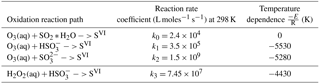
The reaction rates of oxidation by ozone and hydrogen peroxide can be described as a Hoffmann and Calvert (1985):

$$\begin{array}{ll}{\displaystyle }{\mathbb{R}}_{{\mathrm{O}}_{\mathrm{3}}}& {\displaystyle }={\displaystyle \frac{\text{d}\left[{\mathrm{S}}^{\text{VI}}\right]}{\mathrm{d}t}}{\mathrm{|}}_{{\mathrm{O}}_{\mathrm{3}}}=\left(k_{\mathrm{0}}+{\displaystyle \frac{k_{\mathrm{1}}{\mathbb{K}}_{{\mathrm{SO}}_{\mathrm{2}}}}{\left[{\mathrm{H}}^{+}\right]}}+{\displaystyle \frac{k_{\mathrm{2}}{\mathbb{K}}_{{\mathrm{SO}}_{\mathrm{2}}}{\mathbb{K}}_{{\mathrm{HSO}}_{\mathrm{3}}}}{[{\mathrm{H}}^{+}{]}^{\mathrm{2}}}}\right)\\ \text{(4)}& {\displaystyle }& {\displaystyle }\left[{\mathrm{O}}_{\mathrm{3}}\right]\left[{\mathrm{SO}}_{\mathrm{2}}*{\mathrm{H}}_{\mathrm{2}}\mathrm{O}\right],\end{array}$$

$$\begin{array}{}\text{(5)}& {\mathbb{R}}_{{\mathrm{H}}_{\mathrm{2}}{\mathrm{O}}_{\mathrm{2}}}={\displaystyle \frac{\text{d}\left[{\mathrm{S}}^{\text{VI}}\right]}{\text{d}t}}{\mathrm{|}}_{{\mathrm{H}}_{\mathrm{2}}{\mathrm{O}}_{\mathrm{2}}}={\displaystyle \frac{k_{\mathrm{3}}{\mathbb{K}}_{{\mathrm{SO}}_{\mathrm{2}}}}{\mathrm{1}+k_{\mathrm{4}}\left[{\mathrm{H}}^{+}\right]}}\left[{\mathrm{H}}_{\mathrm{2}}{\mathrm{O}}_{\mathrm{2}}\right]\left[{\mathrm{SO}}_{\mathrm{2}}*{\mathrm{H}}_{\mathrm{2}}\mathrm{O}\right],\end{array}$$

where ℝ_A is the reaction rate of the chemical compound “A” and $k_{\mathrm{0},\mathrm{\dots },\mathrm{4}}$ are the reaction rate coefficients. $k_{\mathrm{0},\mathrm{\dots },\mathrm{4}}$ depend on the temperature following a similar relation as for dissociation, Eq. (1). Table C5 shows the values of the reaction rate coefficients and their temperature dependence coefficients.

Equations (4) and (5) return the new concentration of S^VI created in each SD in each time step. Based on the new concentration, the new mass of S^VI and the new dry radius are calculated and the corresponding SD attributes are updated. The dry particle density of 1.8 g cm⁻³ is assumed while evaluating the dry radius from the S^VI mass.

For the typical atmospheric conditions, say pH between 3 and 6 (i.e. [H⁺] between 10⁻³M and 10⁻⁶M), it can be said that the rate of oxidation by H₂O₂ depends very weakly on pH. In contrast, oxidation by ozone depends strongly on pH of the solution and can become very fast if pH is high. For example, increasing pH by 1 unit results in an approximately 100-fold increase in the O₃ reaction rate.

3.4 Initialization

The initial aerosol is assumed to be ammonium bisulfate (NH₄HSO₄), with a dry particle density of 1.8 g cm⁻³. Using the dry particle density and the dry radius of each SD, the initial mass of H⁺, ${\mathrm{NH}}_{\mathrm{4}}^{+}$ and ${\mathrm{SO}}_{\mathrm{4}}^{\mathrm{2}-}$ ions is calculated. The initial mass of other molecules and ions is set to zero and is therefore not in equilibrium with the initial ambient trace gas conditions. For the initial conditions where supersaturation is present in the environment it is advisable to allow for a spin-up period with only condensation/evaporation and the equilibrium chemical processes enabled, to allow the model to reach equilibrium. Such initial conditions are mostly relevant for the kinematic models.

4 Comparison with moving-bin schemes

The PBMC scheme is set to reproduce results from the model intercomparison study by Kreidenweis et al. (2003), where several bulk and moving-bin schemes representing cloud microphysics and aqueous-phase chemistry were tested in an adiabatic parcel model set-up. The parcel model used here is a 0-dimensional model that represents an idealized scenario of a finite volume of air rising adiabatically with a constant vertical velocity. As the parcel of air raises, its temperature decreases leading to supersaturation. This results in activation and further condensational growth of cloud droplets. For the studied oxidation reaction, the presence of liquid water enables aqueous-phase chemical reactions and leads to creation of sulfuric acid within cloud droplets. The collisions between cloud droplets are not included in the parcel simulations to allow an easy comparison with Kreidenweis et al. (2003).

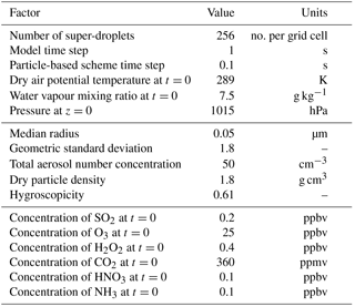
The initial conditions are the same as in Kreidenweis et al. (2003) and are provided for convenience in Table 1.

Table 1 Initial conditions for the adiabatic parcel test.

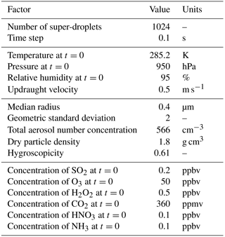
The simulation starts below cloud base (i.e. with subsaturation). The initial aerosol is ammonium bisulfate and the initial aerosol particle size distribution is assumed to be lognormal with one mode

$$\begin{array}{}\text{(6)}& n\left(r_{\text{d}}\right)={\displaystyle \frac{n_{\text{tot}}}{r_{\text{d}}\sqrt{\mathrm{2}\mathit{\pi }}\ln \left({\mathit{\sigma }}_{\text{g}}\right)}}\exp \left(-{\displaystyle \frac{{\left(\ln \left(r_{\text{d}}\right)-\ln \left(\stackrel{\mathrm{‾}}{r_{\text{d}}}\right)\right)}^{\mathrm{2}}}{\mathrm{2}{\ln }^{\mathrm{2}}\left({\mathit{\sigma }}_{\text{g}}\right)}}\right),\end{array}$$

where n(r_d) is the spectral density function of aerosol particle sizes, n_tot is the total aerosol concentration, $\stackrel{\mathrm{‾}}{r_{\text{d}}}$ is median radius, and σ_g is the geometric standard deviation. See Sect. 5.1.6 in Arabas et al. (2015) for the details on how the SD dry and wet radii are initialized.

The parcel model employed in this study uses dry air density ρ_d, dry air potential temperature θ, water vapour mixing ratio r_v, and mixing ratios of ambient trace gases as model variables. In order to calculate ρ_d at each time level (or each height level of the parcel ascent) the model needs to assume a vertical profile of pressure. In the presented simulations the pressure profile is obtained by integrating the hydrostatic equation and assuming that the density of air is constant and equal to 1.15 kg m⁻³. The assumed density is based on the density provided in Table 3 in Kreidenweis et al. (2003). Then, at each level, ρ_d is calculated from the ideal gas law taking into account the current r_v and θ:

$$\begin{array}{}\text{(7)}& {\mathit{\rho }}_{\text{d}}(p,\mathit{\theta },r_{\text{v}})={\displaystyle \frac{p-p_{\text{v}}(p,r_{\text{v}})}{{\text{R}}_{\text{d}}\mathit{\theta }(\frac{p}{p_{\mathrm{1000}}}{)}^{\frac{{\text{R}}_{\text{d}}}{c_{\text{pd}}}}}},\end{array}$$

where: p_v represents the partial pressure of water vapour, p₁₀₀₀ stands for the pressure equal 1000 hPa that comes from the definition of potential temperature, R_d is the gas constant for dry air, and c_pd is the specific heat at constant pressure for dry air. Because the simulated air parcel is assumed to be adiabatic, only the processes resolved by the particle-based scheme can change θ, r_v, and other trace gas mixing ratios. In each model time step, the particle-based microphysics scheme changes θ and r_v according to Eqs. (25) and (26) from Arabas et al. (2015). The changes in the trace gas mixing ratios are resolved following the procedure discussed in Sect. 3.2. It is assumed that the initial mass of dry air within the parcel is 1 kg.

Figure 1 shows the general physical and chemical conditions from the cloud base up to the end of the test run 1.2 km above the cloud base. Two vertical axes are used, representing either the time or the height above the cloud base. Figure 1a shows the liquid water mixing ratio (LWC). The increase in LWC is linear and the LWC reaches above 2 g kg⁻¹ at a height of 1.2 km above the cloud base. Figure 1b shows the total SO₂ concentration (both in gas phase and dissolved in water) in ppb units. The concentration of SO₂ is decreasing due to oxidation taking place in the cloud droplets. Figure 1c shows the water volume weighted average pH of the cloud droplets. The pH near the cloud base is very low due to the acidic nature of the assumed initial aerosol and the small size of the activated cloud droplets. As the drops grow bigger and become more diluted, the average pH increases. Figure 1 compares well with Fig. 1 from Kreidenweis et al. (2003).

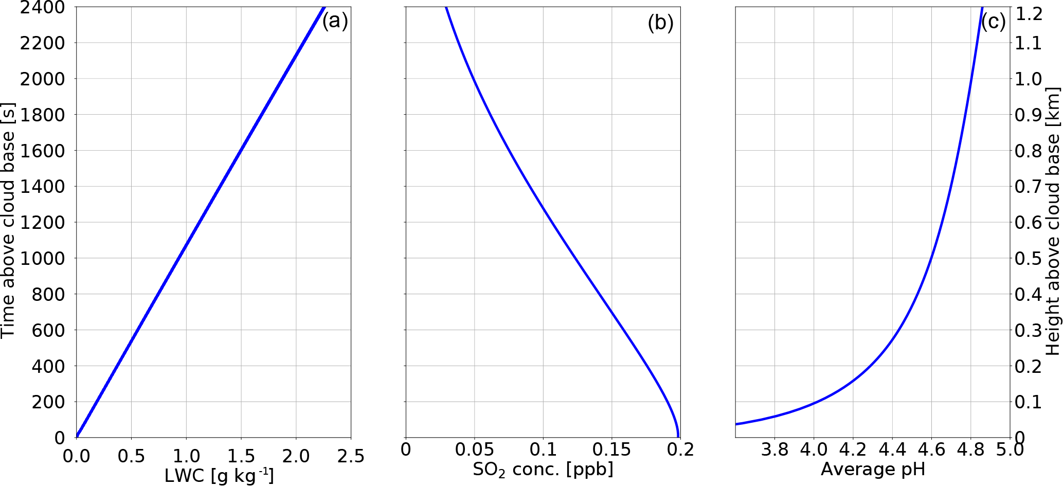
Figure 1 Physical and chemical conditions in the adiabatic parcel model. Panel (a) shows the liquid water mixing ratio (LWC), panel (b) shows the SO₂ concentration (both gas phase and dissolved), and panel (c) shows the water volume weighted average pH of the simulated population of water drops.

At the end of the test simulation, 85 % of SO₂ is converted into S^VI and the final water volume weighted average pH is equal to 4.86. The total sulfate production is 171 ppt with 99 ppt produced by the H₂O₂ reaction path and 72 ppt produced by the O₃ reaction path. Based on Fig. 2 in Kreidenweis et al. (2003), the range of average pH values reported by different size-resolving (moving-bin) schemes was between 4.82 and 4.85, and the range of total sulfate production values was between 170 and 180 ppt. Based on Fig. 3 in Kreidenweis et al. (2003), the production by H₂O₂ ranged between 85 and 105 ppt, and by O₃ between 70 and 85 ppt for the size-resolving schemes. In short, the results from the particle-based scheme are close to the range of values reported by the moving-bin schemes.

The microphysics schemes taking part in the Kreidenweis et al. (2003) intercomparison study reported significant differences between the number of activated cloud droplets. Based on Table 2 in Kreidenweis et al. (2003), the droplet number concentration at the cloud base varied between 275 and 358 cm⁻³. One of the differences between the moving-bin schemes responsible for causing this discrepancy is the different water vapour mass accommodation coefficient α_M leading to different predicted maximum supersaturation. Figure 6 in Kreidenweis et al. (2003) shows that the observed maximum supersaturations were lower (between 0.23 % and 0.26 %) for schemes using high values of α_M (either 0.5 or 1). In contrast, a scheme using α_M=0.042 predicted maximum supersaturation equal to 0.37 %. The particle-based scheme used in this study reports a concentration of 269 cm⁻³ at the level of maximum supersaturation. The maximum supersaturation is equal to 0.27 %. The particle-based scheme assumes α_M equal to unity and therefore fits with the trend of high α_M causing lower supersaturation presented in Fig. 6 in Kreidenweis et al. (2003).

Another cause for the discrepancy between the bin schemes listed in the intercomparison study are the different sizes and locations of bins in different models, see also the discussion in Arabas and Pawlowska (2011). Along those lines, here it is tested how sensitive the particle-based scheme is to the number of SDs. The results of this test are summarized in Fig. 2 showing the cloud droplet concentration at the cloud base (a), the maximum supersaturation (b), the average pH (c) and the total sulfate production (d). The results are plotted against the logarithm of base 2 of the number of SDs in the computational domain (meaning that “0” represents one SD and “10” represents 1024 SDs). All values seem to converge for SD numbers greater than 64. The average pH, maximum supersaturation, and total sulfate production do not change for those four test-runs. The concentration of droplets at the cloud base varies little (between 269 and 281 cm⁻³). The concentrations from simulations with SD number between 512 and 1024 vary between 274 and 269 cm⁻³. For SD numbers between 32 and 64 there are insignificant changes in the maximum supersaturation. The values of pH vary by 0.01 and the total sulfate production increases by 1 ppt. There are, however, large differences between the number of droplets at the cloud base (between 281 and 332 cm⁻³). This confirms the observations from Kreidenweis et al. (2003) that the predicted cloud droplet number concentration strongly depends on the representation of the size distribution of modelled aerosol particles and cloud droplets and that this may become a major source of uncertainties in the microphysics representation. Decrease in the SD number below 32 leads to a big variance in the cloud droplet concentration as well as other parameters.

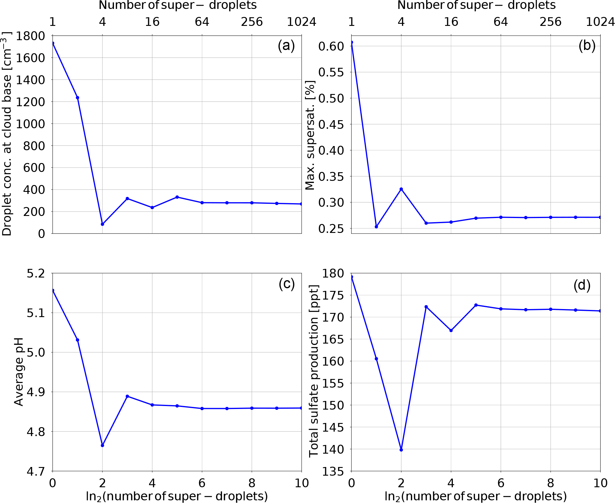
Figure 2 Results of the convergence test for the adiabatic parcel simulations. All panels show how a given parameter depends on the number of SDs (shown on the abscissa as the logarithm of base 2 of the number of SDs). Panel (a) shows the cloud droplet concentration at the cloud base, panel (b) the maximum supersaturation, panel (c) the water volume weighted average pH at the end of simulation, and panel (d) the total sulfate production.

Figure 3 shows the simulated modification of the aerosol size distribution. The red line depicts the initial distribution and the green line shows model state at the end of the adiabatic parcel test. For convenience, Fig. 3 uses both logarithmic (left panel) and linear (right panel) scales on the axes. The change in the aerosol size distribution is caused by oxidation. The aerosol particles that are too small to become cloud droplets are not affected by aqueous-phase oxidation and do not grow in size. The large aerosol particles grow in size due to S^VI production during oxidation, but the increase in size is small compared to their initial size. The smallest activated aerosol particles are affected most by oxidation. The increase in their size due to the produced S^VI is the largest compared to their initial size. In short, oxidation produces a “gap”, often labelled the “Hoppel minimum”, between the CCN processed by the cloud and the smaller unactivated aerosol particles.

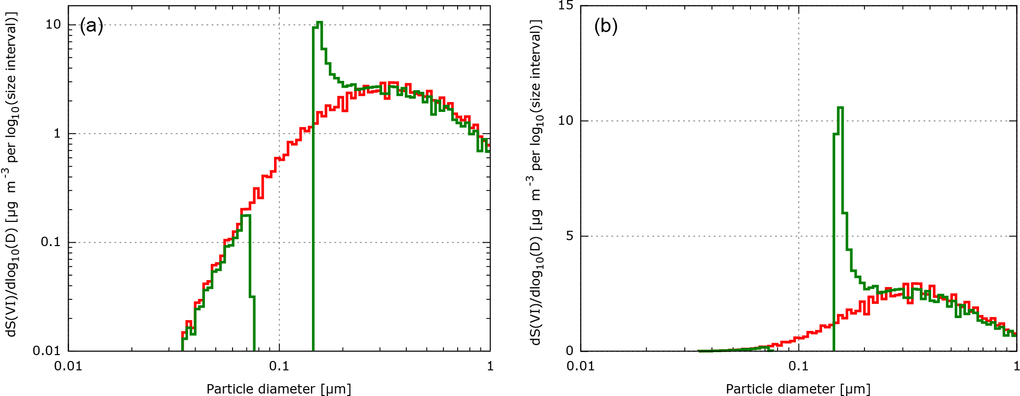
Figure 3 Modification of the dry aerosol sulfate mass. The red line shows the initial condition and the green line shows the final model state. The left panel uses a logarithmic scale and the right panel uses a linear scale.

The effect of in-cloud sulfate production on the aerosol particle size distribution presented in Fig. 3, combined with other tests presented in this section, documents the correctness of the implementation of the aqueous chemistry in the particle-based scheme. The formation of the “Hoppel minimum” was reported by many observational studies, see Hoppel et al. (1994), Bower et al. (1997), and Hudson et al. (2015). Figure 3 compares well with the aerosol size distribution plots from the intercomparison study shown in Fig. 9 in Kreidenweis et al. (2003). Other numerical schemes also reported the formation of the Hoppel minimum, see for example Flossmann (1994), Feingold and Kreidenweis (2000, 2002), and Ovchinnikov and Easter (2010). The work by Cantrell et al. (1999) shows that the maximum supersaturation and the cloud droplet concentration in the clouds which processed the aerosol particles can be inferred based on the location of the aerosol size distribution minimum.

5 Example simulations

5.1 2-D kinematic model

The kinematic model mimics a single 2-D eddy spanning a stratocumulus cloud deck and a boundary layer below it. The model is based on a test scenario from the 8th International Cloud Modeling Workshop (Muhlbauer et al., 2013). The velocity field is prescribed as in Szumowski et al. (1998), Morrison and Grabowski (2007), and Rasinski et al. (2011). The same model was used when presenting the initial release of libcloudph++, see Sect. 2 in Arabas et al. (2015) for details of the model formulation. The kinematic model is based on the open-source library of parallel MPDATA-based solvers for systems of generalized transport equations, see Jaruga et al. (2015). The temperature, moisture, and trace gas fields are discretized on the Eulerian grid and are advected using the prescribed velocity field. Then, the model variables are passed to the PBMC scheme, where the microphysical and chemical processes are resolved. Finally, the source and sink terms due to microphysics and chemistry are calculated and applied in each model grid cell as described in Sects. 2 and 3.

Table 2 Initial conditions for the base case of the 2-dimensional kinematic model.

The collisions between water drops are represented using the geometric kernel with collision efficiency for big drops (i.e. radius greater than 20 µm) from Hall (1980) and for small droplets (i.e. radius smaller than 20 µm) from Pinsky et al. (2008). For big drops, the collision efficiencies were obtained from the fit to measurements, see Hall (1980). For small droplets, the collision efficiencies were based on numerical simulations taking into account turbulence typical for stratocumulus clouds, see Pinsky et al. (2008). The collision efficiencies are provided via a look-up table for different drop sizes.

The initial conditions are summarized in Table 2. The computational domain size is 1.5 km in both directions and the computational grid is composed of 75×75 cells of equal size (the grid lengths are 20 m) and is periodic in the horizontal direction. The initial air density profile corresponds to the hydrostatic equilibrium with the pressure of 1015 hPa at the bottom of the domain. At the beginning of the simulation it is assumed that there is no condensed water, and the initial profiles of θ and r_v are constant with altitude. To keep the simulation set-up simple and due to a relatively low vertical extent of the computational domain, the initial trace gas volume fractions are also assumed to be constant with altitude. This unrealistic initial condition results in very high initial supersaturation in the upper part of the domain. As a consequence a 10⁵ s (∼2 h 45 min) spin-up period is necessary to allow for the simulated water drops to reach equilibrium with their environment. During the spin-up only the reversible processes (condensation and evaporation, dissolving of trace gases, and dissociation into ions) are allowed and the supersaturation is limited to 5 % (relative humidity RH=1.05). After spin-up the simulations are run for 30 min. The chosen simulation time is enough to deplete the SO₂ available in the cloudy part of the domain as well as to create precipitation.

Similar to the adiabatic parcel test, the initial aerosol is ammonium bisulfate and the aerosol particle size distribution is lognormal with one mode. The initial condition for trace gases is defined in terms of volume fractions and then translated to mixing ratios that serve as the model variables. The initial SO₂, O₃, and H₂O₂ volume fractions are taken from the simulation set-up used in Ovchinnikov and Easter (2010). The values for SO₂ and O₃ are based on the measurements from the MASE campaign (Wang et al., 2008) and the value for H₂O₂ is based on the representative values for the eastern Pacific Ocean (Genfa et al., 1999). The NH₃, HNO₃, and CO₂ volume fractions are the same as in the parcel test from Sect. 4.

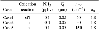
The set-up detailed in Table 2 corresponds to “very clean conditions” (i.e. low aerosol particle concentrations). The initial aerosol particle sizes are also relatively small. Three additional simulation cases are studied to check the sensitivity of the model to different conditions. In case1 the reversible chemical processes are allowed, but the oxidation reaction is prohibited. In case2 the initial volume fraction of NH₃ is increased and in case3 the initial aerosol size distribution is changed. The conditions for all the sensitivity simulation cases are summarized in Table 3.

Table 3 Initial conditions for sensitivity test cases of the 2-dimensional kinematic model. Specified are aqueous-phase chemistry choice, initial volume fraction of NH₃, mean radius of the assumed lognormal aerosol particle size distribution r_d, total aerosol concentration n_tot, and geometric standard deviation σ_g. Other parameters for each case are the same as in the base case (Table 2) The parameters that distinguish each sensitivity test case are marked in bold.

As discussed in Flossmann (1994), the initial chemical scenario is idealized. For instance, although the initial conditions represent a clean maritime environment, the set-up lacks sea salt aerosol particles. As discussed by Twohy et al. (1989), sea salt aerosol particles are alkaline, which may in turn increase the pH of water drops and thus affect the oxidation rate. On the other hand, a study by von Glasow and Sander (2001) indicates that alkaline sea salt particles are quickly converted to acidic due to the uptake of HCl vapour. More importantly, including sea salt would result in aerosol particles with very different hygroscopicity values (Petters and Kreidenweis, 2007). Including sea salt would also result in the initial bimodal size distribution with one mode representing smaller ammonium bisulfate aerosol particles and the second mode representing larger sea salt particles. In general, including sea salt should result in a very different condensational growth of aerosol particles. The set-up used in this study also lacks other particles containing sulfate, such as ammonium sulfate or sulfuric acid aerosol particles.

The initial aerosol size distribution parameters are based on the test cases studied in Feingold and Kreidenweis (2002). The discussion presented in their study introduced two regimes for oxidation with regard to the mean aerosol size $\stackrel{\mathrm{‾}}{r_{\text{d}}}$ and precipitation: (i) for a relatively small initial $\stackrel{\mathrm{‾}}{r_{\text{d}}}$ production of sulfate enhances precipitation, and (ii) for a relatively big initial $\stackrel{\mathrm{‾}}{r_{\text{d}}}$ production of sulfate suppresses precipitation. The overall impact depends strongly on the initial concentration of aerosol particles, see Feingold and Kreidenweis (2002) for the discussion. The short simulation time used in this study hinders analysis of the impact of oxidation on the overall precipitation. The work presented here focuses on the evolution of aerosol particle sizes and pH values of cloud and drizzle droplets. Future large eddy simulations should focus on the impacts of aqueous chemistry on precipitation, cloud lifetime, and cloud dynamics.

The kinematic set-up precludes any links between cloud microphysical processes and dynamics of the air motion. The set-up limits the study to the smooth velocity and therefore smooth saturation fields and prevents mixing between air parcels with different trajectories and properties. On the other hand, the kinematic set-up has low computational cost and allows for easy testing and sensitivity analysis. Prescribing the velocity ensures that all changes to the aerosol particle and water drop size distributions are caused by the cloud microphysics and aqueous-phase chemistry alone. Moreover, the kinematic set-up allows for a straightforward selection of the updraught and downdraught regions, further simplifying the analysis of the microphysical processes.

5.2 Results

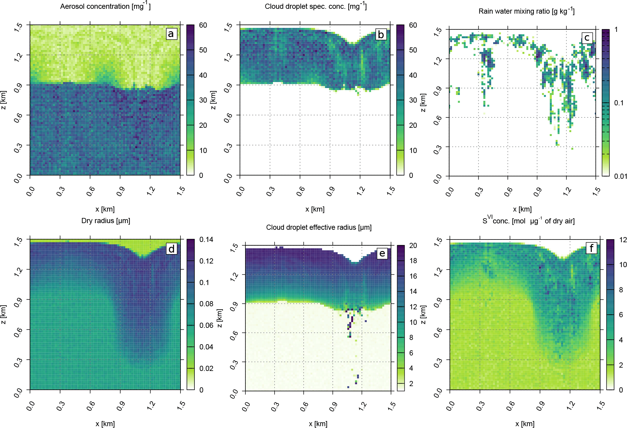
Figure 4 The base case set-up (see Table 2). All panels depict the model state after 30 min simulation time (excluding the spin-up) and show unactivated aerosol concentration (a), cloud droplet specific concentration (b), rain water mixing ratio (c), mean dry radius (d), cloud droplet effective radius (e), and concentration of S^VI molecules (f). The three thresholds for particle radii are unactivated aerosol <1 µm; 1 µm < cloud <25 µm; rain >25 µm. Note the logarithmic scale for the rain water mixing ratio plot.

Figure 4 shows the model state after 30 min of simulation from the base case (see Table 2). Figure 4a shows the concentration of the unactivated aerosol particles (defined as the SDs with wet radius smaller than 1 µm). The lower part of the plot (below 900 m) shows cloud-free conditions and corresponds to the initial concentration of aerosol particles. The upper part of the plot shows the interstitial aerosol particles, i.e. those in-cloud aerosol particles that did not activate. The difference between the upper and lower parts of Fig. 4a shows the impact of nucleation scavenging on aerosol population. The regions with slightly higher concentration of the in-cloud aerosol particles near the cloud base correspond to regions with low vertical velocities, lower supersaturations, and thus lower concentrations of the cloud droplets. Figure 4b shows the concentration of the cloud droplets (defined as the SDs with wet radii between 1 and 25 µm). It is nearly constant with height, that agrees with the observations in stratocumulus clouds (Pawlowska et al., 2000). The regions with lower cloud droplet concentrations correspond to the regions with drizzle (see Fig. 4c). Figure 4c shows the rain water mixing ratio (water drops with wet radius greater than 25 µm) using a logarithmic colour scale. Rain forms quickly in the simulation due to the relatively high values of cloud droplet radii after the spin-up caused by the low initial aerosol particle concentration. The footprint of precipitation can be seen in Fig. 4b and f where the cloud droplet concentration is depleted in regions of drizzle. Figure 4d shows the mean dry radius of all particles (both the aerosol particles and water drops). The mean dry radius is increasing due to oxidation. In the updraught (left-hand side of panel d) the environmental aerosol particles that have not been affected by cloud are advected into the cloudy region. Once the cloud droplets are formed, the aqueous-phase oxidation starts to produce sulfate and changes the CCN size distribution. In the downdraught (right-hand side of panel d) cloud droplets are advected out of the cloud and they evaporate. The cloud-processed CCN are returned to the environment and change the ambient air aerosol particle size distribution. Figure 4e depicts the cloud droplet effective radius. As expected, the effective radius increases with height. At the top of the cloud the effective radius reaches 20 µm, which is linked to the small cloud droplet concentration. High effective radii imply efficient drizzle production after the spin-up (usually water drop radius ∼12 µm is reported as the threshold value for efficient collisions between water drops and the production of precipitation, for example Pawlowska and Brenguier, 2003; Rosenfeld and Gutman, 1994). Figure 4f shows the concentration of S^VI molecules (all molecules containing sulfur at +VI oxidation state) and represents molecules from the initial ammonium bisulfate (NH₄HSO₄) aerosol and the molecules created during oxidation. It corresponds to the mean dry radius plotted in Fig. 4d. Additionally, some effects of collisions and precipitation can be seen when comparing the irregular features from Fig. 4f with rain water mixing ratio in Fig. 4c. Precipitation displaces the largest water drops, which causes the irregular distribution of S^VI molecules in cloudy grid cells. Figure 4f also shows that the particle-based scheme can track the dissolved chemical compounds in the evaporating rain drops below the cloud base.

Figure 4b, d, e, and f show a layer of very clean air above the cloud which is caused by sedimentation of cloud droplets. In the downdraught region, the prescribed velocity field advects the clean layer into the domain. This feature is not present in the aerosol concentration plot (Fig. 4a) because the clean layer contains small aerosol particles with small sedimentation velocity. The depicted clean layer is an artifact caused by the prescribed velocity field and the absence of aerosol sources in the computational domain. The relatively short simulation time is chosen to minimize the impact of the clean layer on the simulation.

Figure 5 The liquid water volume weighted average pH from the base case (a), case1 (b), case2 (c), and case3 (d). See Tables 2 and 3 for a definition of simulation set-ups.

Figure 5 shows the liquid water volume weighted average pH in each computational grid cell from the base case (a) and sensitivity test cases (b–d). In order to better adjust the colour scale to the in-cloud pH variability, pH values below 3 that correspond to very acidic aerosol particles below the cloud base have been clipped. Figure 5 captures the pH of cloud droplets as well as the pH of some evaporating rain drops below the cloud base. The droplets in the downdraught of Fig. 5a are more acidic due to S^VI created during aqueous-phase oxidation. For the base case, Fig. 5a, pH increases with height above the cloud base. Initially the water drops are very acidic, but as they grow in size they become more diluted. Even though S^VI is created during oxidation, the average pH still increases with height due to dilution. The same behaviour is shown in the adiabatic parcel tests discussed in Sect. 4 and shown in Fig. 1. The increase in pH with height is also observed in a 1-dimensional model representing processing of sulfur in small cumuli in marine environment used by Alfonso and Raga (2002). Due to the pH variability shown in Fig. 5a, oxidation by O₃ happens mostly near the cloud top in the base case. As discussed in Sect. 3.3, the rate of oxidation by O₃ increases significantly with increasing pH (see Eq. 4), whereas oxidation by H₂O₂ depends very weakly on the acidity (Eq. 5). The study by Walcek and Taylor (1986) also reported that the pH of droplets increased with height due to dilution despite the production of sulfuric acid. In turn, increased pH promotes oxidation by O₃ in the upper parts of the cloud, whereas oxidation by H₂O₂ dominates in lower parts of the cloud, according to their study.

Case1 shown in Fig. 5b represents a hypothetical “no oxidation” scenario where all physical and chemical conditions are the same as in the base case, the reversible chemical processes are allowed, and the oxidation reaction is prohibited. The scenario without oxidation is overall less acidic than the base case (Fig. 5a). Additionally, without oxidation there is no difference between the pH values in the updraught and downdraught in Fig. 5b. Without oxidation, all the chemical processes are reversible and the dissolved chemical compounds are outgassed to the atmosphere as the cloud droplets evaporate in the downdraught.

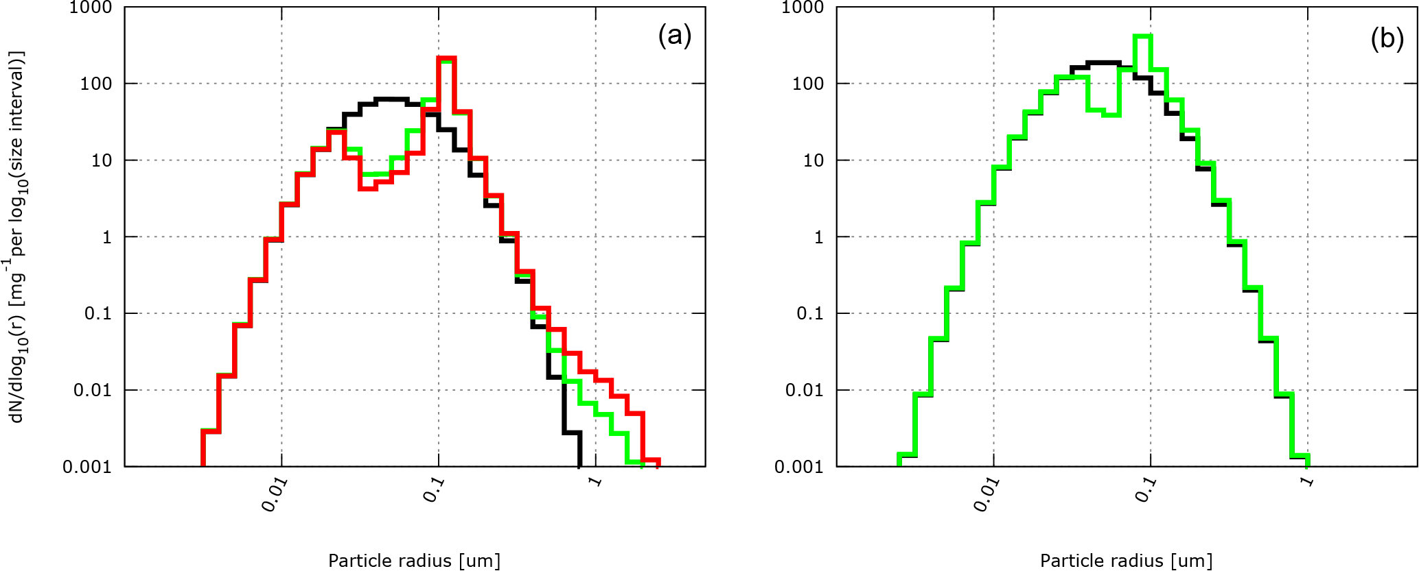
Figure 6 The size distributions of dry radii for the base case (a) and case3 (b). The initial dry radius size distribution is marked in black, the final dry radius size distribution from grid cells with r_c>0.01 g kg⁻¹ in green, and from grid cells with r_r>0.01 g kg⁻¹ in red. See Tables 2 and 3 for a definition of simulation set-ups.

Case2 differs from the base case by increasing the initial NH₃ volume fraction from 0.1 to 0.4 ppbv (see Tables 2 and 3). Because the initial aerosol particle size distribution is the same as in the base case, the mean aerosol and droplet sizes and concentrations at the end of the simulation are not different from the base case (not shown). Figure 5c shows the liquid water volume weighted average pH for case2. The average pH in case2 (Fig. 5c) is higher than in the base case (Fig. 5a), that is, both cloud droplets and rain drops are less acidic in case2 than in the base case. In contrast to the base case, in the updraught (left-hand side of the plots), the pH in case2 actually decreases with height above the cloud base. This is because the higher initial NH₃ volume fraction increases its uptake and counters the low pH values caused by the initial acidic aerosol particles, see Eq. (2). Then, as the water drops are advected upwards, oxidation produces sulfuric acid and the average pH decreases. Near the cloud top, the NH₃ is degassed back to the environment. The case2 results are in agreement with the trajectory ensemble model simulations by Zhang et al. (1999). In their study, the initial aerosol size distribution is the same as in the base case and case2. However, their initial trace gas volume fractions are much higher and aim to represent a “moderately polluted marine environment” (their base case NH₃ volume fraction is 10 times larger than the base case value assumed here). As in case2 presented here, the high initial NH₃ volume fractions in Zhang et al. (1999) increase the pH near the cloud base and promote oxidation by O₃ during the first minutes after the simulated parcels entered the cloud. Because the sulfuric acid was produced, the pH dropped and oxidation by H₂O₂ becomes dominant in the higher regions of the cloud, as reported in their study.

Case3 increases the initial aerosol concentration to 150 cm⁻³, while keeping all other initial conditions the same as in the base case (see Tables 2 and 3). In general, higher initial aerosol particle concentration results in higher cloud droplet concentrations. This in turn creates smaller cloud droplet effective radii that virtually prohibits the onset of precipitation during the 30 min simulation time (not shown). Figure 5d shows the liquid water volume weighted average pH for case3. Similar to the base case (Fig. 5a), the pH increases with height due to the dilution and the downdraught droplets are more acidic due to the ongoing oxidation. However, case3 is more acidic than the base case because the overall droplet sizes are smaller and they are therefore less diluted.

At the end of the base case simulation, 18 % of the total available S^IV is oxidized. As a result, 0.14 µg m³ of the dry particulate matter is created during oxidation per cubic metre of air (an average value for the whole computational domain reported in relation to the dry air volume). In total, 40 % of the final dry particulate matter is created due to oxidation and 60 % originates from the initial aerosol mass. The oxidation is a significant source of the dry particulate matter because the initial aerosol mass is very low (only 0.21 µg m³ dry air). Oxidation by H₂O₂ is the dominant path: 92 % of S^VI originates from S^IV oxidation by H₂O₂. More alkaline conditions of case2 enhance the efficiency of oxidation. At the end of case2, 21 % of available S^IV is oxidized. As a result, oxidation produces 0.16 µg of dry particulate matter per cubic metre of dry air (average over the whole computational domain). For case2, 44 % of the final dry particulate matter is created due to oxidation and 56 % originates from the initial ammonium bisulfate aerosol. Similar to the base case, the significance of oxidation as a source of dry particulate matter is caused by a very low initial aerosol mass. Due to more alkaline conditions, oxidation by O₃ becomes more important than in the base case. At the end of the case3 simulation, 39 % of the S^VI originates from S^VI oxidation by O₃ and 61 % by H₂O₂. In contrast, more acidic conditions of case3 hinder the O₃ reaction path. Virtually all molecules of sulfate that are created during oxidation are oxidized by H₂O₂. As a result, the conversion of sulfur to sulfate is slightly less effective in case3. At the end of the case3 simulation, 17 % of available S^IV is oxidized. As a result, 0.13 µg of dry particulate matter is created per cubic metre of dry air. At the end of case3 simulation, 17 % of the dry particulate matter is created by oxidation and 83 % originates from the initial aerosol. The initial aerosol mass is larger in case3 than in the base case due to the higher initial aerosol concentration (case3 contains initially 0.61 µg m³ of dry particulate matter). Due to the simple kinematic set-up chosen in this study the values reported here cannot be treated as representative of the atmospheric conditions. They are shown to allow comparison between the base case and the sensitivity test cases.

Finally, the impact of collisions and aqueous-phase oxidation of sulfur on the aerosol and water drop size distributions is examined. For this purpose, the aerosol particle size distributions from the base case (Fig. 6a) and case3 (Fig. 6b) are compared. The black line represents the initial aerosol size distribution, and the green and red lines represent the final aerosol size distribution for the in-cloud (r_c>0.01 g kg⁻¹) and precipitating (r_r>0.01 g kg⁻¹) grid cells, respectively. The two cases are chosen because they have different initial aerosol size distributions. In both cases the cloud-processed aerosol size distributions (green and red lines) have a bimodal shape. This is a footprint of oxidation that creates the Hoppel minimum in the dry radius size distribution. The same effect is obtained in the adiabatic parcel tests discussed in Sect. 4 and shown in Fig. 3. Moreover, the efficient collisions between water drops in the base case create a tail of bigger aerosol sizes in Fig. 6a. The effect is stronger for the precipitating grid cells (red line). In case3 fewer collisions between water drops occur than in the base case and therefore no precipitation and no tail of big aerosol particles is created. Also, in case3, the change in size distribution of aerosol particles caused by oxidation is smaller because the produced sulfate is divided among a larger number of aerosol particles.

6 Summary and outlook

The work presented here describes an extension of the libcloudph++ library that allows us to represent the aqueous-phase chemical reactions within water drops in the particle-based microphysics scheme. The extension covers the aqueous-phase oxidation of sulfur to sulfate. The modular way in which the library is implemented along with the provided documentation should allow, if needed, further development to cover more chemical compounds and reactions. The particle-based microphysics and chemistry scheme is used in 0-dimensional and 2-dimensional modelling set-ups. The former set-up tests the new scheme against the previous numerical studies that used moving-bin microphysics and aqueous-phase chemistry schemes. The latter set-up focuses on the cloud effects on the aerosol particle size distribution (cloud-aerosol processing). Additionally, the changes in the programming interface due to the aqueous chemistry extension are described in Sect. A in the Appendix. Section B in the Appendix completes the description with a list of chemical constants used in the library and chemical reactions included.

The models used in this study to test the chemistry scheme provide a simplified view of the macrophysical cloud properties. They enable testing of the particle-based scheme but do not provide a good balance between the representation of cloud microphysics and dynamics. As a next step, the particle-based scheme needs to be coupled to an eddy-resolving model. This would allow quantifying how microphysical and chemical processes affect precipitation in the model and how they affect the cloud lifetimes simulated by the model.

Appendix A: Programming interface

The programming interface of the particle-based microphysics scheme of libcloudph++ is presented in Sect. 5.2. in Arabas et al. (2015). Here, additional information related to the new aqueous-phase chemistry scheme is provided. The libcloudph++ is implemented in C++ and therefore some nomenclature related to this programming language is used. For a thorough introduction to the C++ programming language, see Stroustrup (2013).

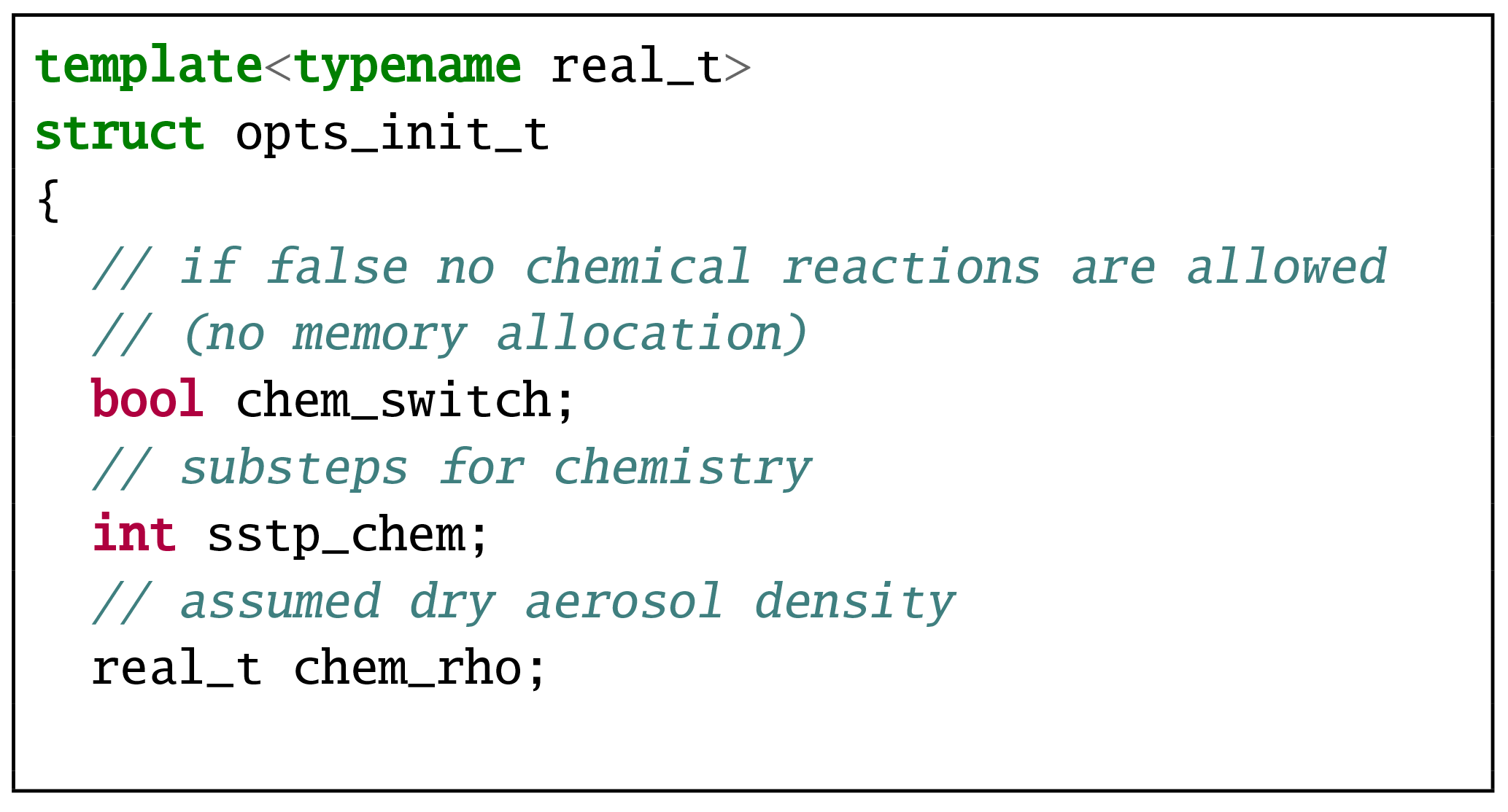
The aqueous chemistry module is implemented as an optional extension to the particle-based microphysics scheme in libcloudph++. It uses the same libcloudphxx::lgrngn namespace as the original scheme. Again the template parameter real_t selects between floating point formats of simulations. The particle-based microphysics scheme options are grouped into the structure named lgrngn::opts_t. The chemistry module adds three Boolean fields to this structure: chem_dsl, chem_dsc, and chem_rct, see code listing in Fig. A1. When set to true by the user, they switch on dissolving of trace gases into water drops, dissociation of chemical compounds in water drops, and oxidation reaction, respectively. The parameters in lgrngn::opts_t can be changed during simulation. For example during the 2-dimensional kinematic simulations from Sect. 5, oxidation is enabled by setting the chem_rct parameter to true at the end of spin-up. Other parameters that cannot be changed during simulation are encapsulated in the lgrngn::opts_init_t structure. The chemistry module adds three fields to this structure: (i) the Boolean chem_switch field that enables memory allocation for additional variables needed for chemistry representation, (ii) the integer sstp_chem field that defines the number of sub-steps to be carried out in aqueous chemistry calculations, and (iii) the real_t chem_rho field that defines the dry aerosol density, see code listing in Fig. A2.

Figure A1 lgrngn::opts_t definition.

Figure A2 lgrngn::opts_init_t definition.

Figure A3 lgrngn::chem_species_t definition.

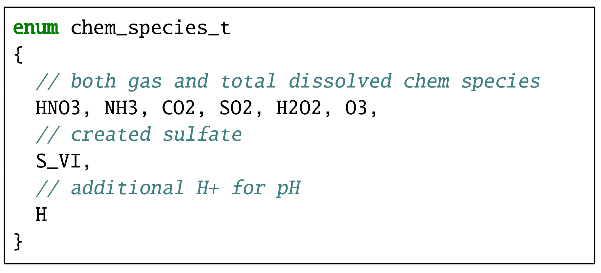
The names of chemical compounds available in the aqueous-phase chemistry module are stored in the chem_species_t enum, see code listing in Fig. A3. The state of all variables used by the particle-based scheme is stored in an instance of the lgrngn::particles_t structure shown in the code listing in Fig. A4. The second template parameter of that structure selects between CPU and GPU calculations (Arabas et al., 2015). The initialization, time stepping, and output from the particle-based scheme are done using the methods of the lgrngn::particles_t structure. Their signatures are provided in the code listing in Fig. A4.

The init() method performs initialization and should be called first. As discussed in Arabas et al. (2015), the first three arguments are obligatory and should point to the dry air potential temperature, water vapour mixing ratio, and dry air density fields of the driver model that uses the libcloudph++. The next three arguments should point to the Courant number field components. They are optional and depend on the dimensionality of the solved problem. For example, for the parcel model tests from Sect. 4 none are necessary, whereas for the 2-dimensional kinematic model from Sect. 5 two arguments are specified in order to describe the velocity field. The last argument of init() is a map with keys from the chem_species_t enum and values pointing to the corresponding trace gas mixing ratio fields from the driver model. This is an optional argument for simulations with aqueous-phase chemistry.

During time stepping, the particle-based scheme computations are performed by the step_sync() and step_async() methods. The first one gathers all the processes that affect the driver model fields (such as condensation/evaporation or aqueous-phase chemistry) and the second one gathers all the processes that can be calculated asynchronously (for example collisions or sedimentation). The list of arguments of the step_sync() method is extended by the chemistry module. Similar to the init() method, a map linking the chem_species_t enum items with the driver model mixing ratio fields needs to be provided as the last optional argument. The particle-based scheme overwrites the driver model fields during simulation. The signature of the step_async method is not changed by the new chemistry module.

Figure A4 lgrngn::particles_t definition.

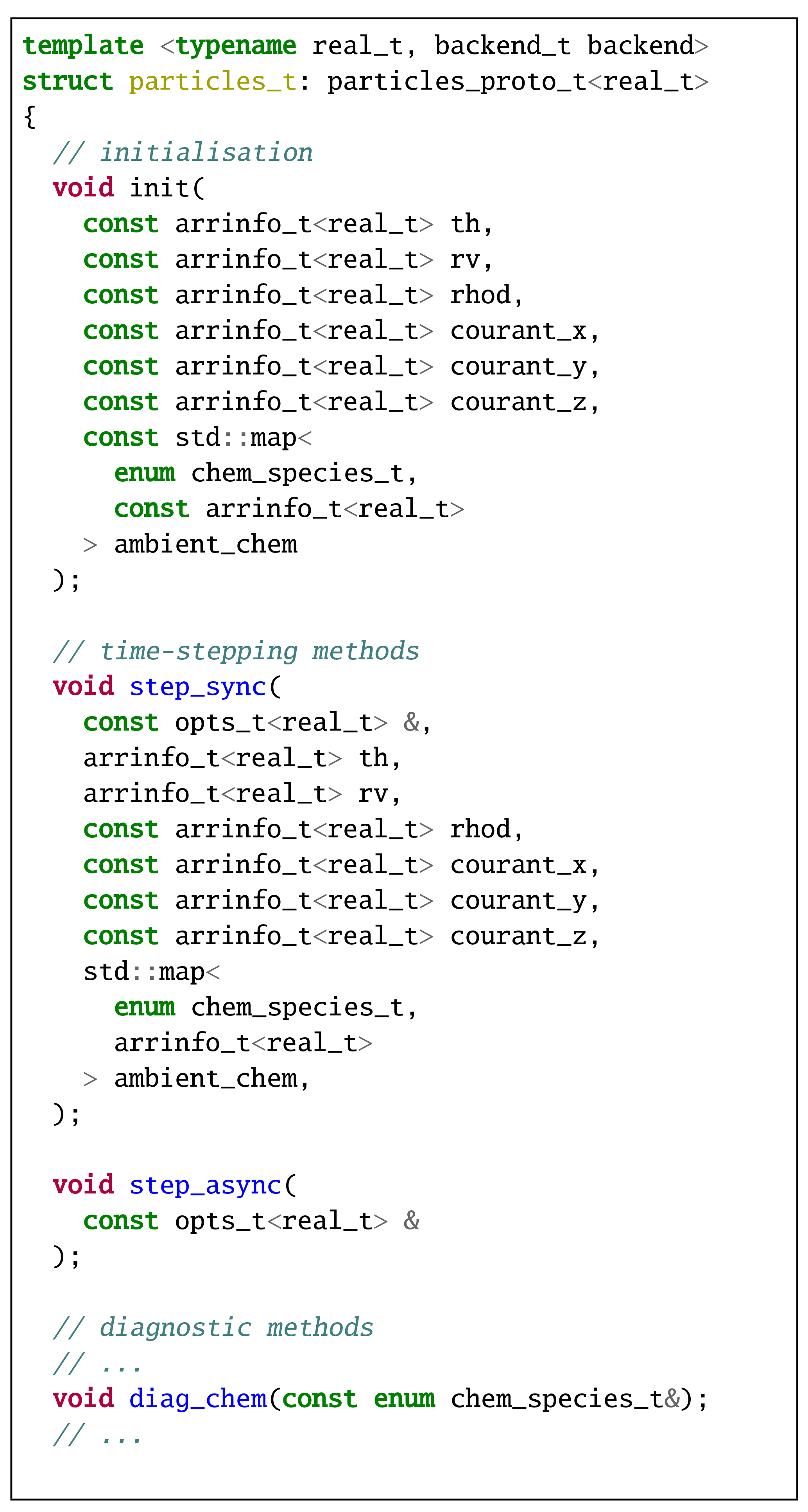
As discussed in Arabas et al. (2015), the lgrngn::particles_t structure provides many methods for obtaining statistical information on the SD parameters (prefixed with diag). The chemistry model adds the diag_chem method to them that outputs the total mass of a chemical compound dissolved into droplets. The chemical compound is selected using the chem_species_t enum items. See the discussion in Sect. 5.2 in Arabas et al. (2015) for the details on how to select the size ranges of droplets specified for output or how to output other statistical parameters.

Appendix B: List of chemical compounds and constants

Table B1 Glossary.

Appendix C:

Table C1 Chemical compounds considered in this work.

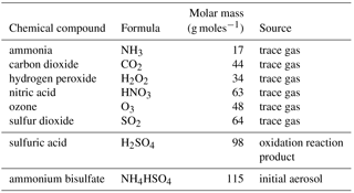
Table C2 Dissociation constants and their temperature dependence coefficients (Kreidenweis et al., 2003). Dissociation of H₂SO₄ is taken from Table 7A.1 in Seinfeld and Pandis (2016).

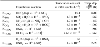
Table C3 Dissolution constants and their temperature dependence coefficients (Kreidenweis et al., 2003).

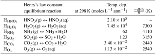
Table C4 Diffusion constants (Massman, 1998; Tang et al., 2014) and accommodation coefficients (Kreidenweis et al., 2003) for relevant chemical compounds.

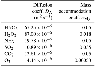
Table C5 Reaction rate coefficients and their temperature dependence coefficients (Kreidenweis et al., 2003).