MONKI: a three-dimensional Monte Carlo simulator for transfer of polarised light in planetary atmospheres

Spectropolarimetry is a powerful tool for characterising planetary atmospheres and surfaces. For the design and operation of spectro(polari)metric instrumentation, numerically simulated signals of the measured radiation are essential. We present MONKI (Monte Carlo KNMI), an efficient and accurate Monte Carlo radiative transfer code written in Fortran. MONKI computes total, linearly polarised, and circularly polarised radiances reflected by and transmitted through planetary atmospheres, fully accounting for the polarisation of light in all orders of scattering. Unlike classical Monte Carlo approaches that rely on post-sampling weight corrections and can therefore produce rare but disproportionately large photon weights, MONKI samples scattering directions from the full polarisation-dependent distribution, consistently in both forward and backward Monte Carlo modes. We provide the corresponding theoretical framework in the appendices. Because of this exact polarised sampling approach, the code converges robustly for optically thick and/or strongly polarising atmospheres. MONKI can handle horizontally homogeneous atmospheres as well as atmospheres with horizontal inhomogeneities, such as three-dimensional (3D) patchy clouds. We validate MONKI through comparisons with other radiative transfer codes. Finally, we present sample simulations of sunlight reflected by the Earth and Venus, and explain the total and polarised radiance features by analysing the altitudes at which photons are scattered. We conclude that MONKI is a versatile and accurate tool for simulations and detailed analyses of total and polarised light emerging from the atmospheres of the Earth, Venus, and, in principle, any other planet.

1 Introduction

Sunlight and, more generally, starlight from solar-type stars, can be considered to be unpolarised when integrated over the disk (Kemp et al., 1987). This light becomes (partially) polarised when it is scattered by the particles constituting a planetary atmosphere. Measuring the degree of polarisation, P, of the scattered light, i.e., the fraction of polarised radiance with respect to the total radiance, is a powerful tool to characterise planetary atmospheres because the scattering angle and wavelength dependence of P are very sensitive to the composition, size, and shape of the scattering particles (Hansen and Travis, 1974). If a planetary atmosphere is bounded below by a surface, light that has been reflected by the surface can also influence the polarisation of the light that is reflected by the planet at the top of the atmosphere (TOA), depending on optical properties of the surface. In particular, Fresnel reflection by liquid surfaces (water on Earth, but hydrocarbons on Titan) or leaves of vegetation can strongly polarise the light (see e.g. Mishchenko and Travis, 1997; Vanderbilt et al., 1985). Additionally, since P is a relative measure, it is insensitive to various instrumental errors and to uncertainties in the total flux of the light that is incident at TOA.

An example of an Earth-observation satellite instrument dedicated to measuring the degree of polarisation was the POLarisation and Directionality of the Earth's Reflectances (POLDER) imager (Deschamps et al., 1994). With multi-angular polarisation observations across three spectral bands, it provided an alternative for the retrieval of cloud droplet sizes to traditional methods that relied solely on total radiances (Breon and Doutriaux-Boucher, 2005), and improved the capability to characterise aerosols above liquid water clouds (Waquet et al., 2013). In February 2024, NASA launched the Plankton, Aerosol, Cloud, Ocean Ecosystem (PACE) satellite (Werdell et al., 2019), carrying the Hyper-Angular Rainbow Polarimeter-2 (HARP-2) (McBride et al., 2024) and the SPEXone spectropolarimeter (van Amerongen et al., 2019), enabling accurate global polarisation measurements of aerosols and clouds to better quantify their impact on radiative forcing. On 13 August 2025, the MetOp-SG-A1 (Meteorological Operational Satellite – Second Generation A1) was launched successfully carrying the Multi-Viewing Multi-Channel Multi-Polarisation Imaging (3MI) instrument (Marbach et al., 2015), and the Multi-Angle Polarimeter (MAP) on the Copernicus Anthropogenic Carbon Dioxide Monitoring (CO2M) mission is scheduled for launch in 2027 (Spilling and Thales, 2021).

Polarimetry has also proven its strength in characterising other solar system bodies than the Earth (see Bagnulo et al., 2024, and references therein). A famous example is the characterisation of Venus's main cloud deck by Hansen and Hovenier (1974), who found that the droplets consist of a ∼ 75 % H₂SO₄ mixture with water, and that their sizes are described by a narrow distribution and effective radii of ∼ 1 µm. They achieved this characterisation using ground-based polarisation measurements of Venus (spatially unresolved, thus integrated across the planet's disk) at a number of wavelengths and a range of planetary phase angles (that is, the angles between Earth, Venus and the Sun) collected over decades by several different observers. ESA's upcoming Venus orbiter EnVision (Ghail et al., 2021), planned for launch in 2032, will carry VenSpec-H (Neefs et al., 2025), a near-infrared spectrometer that will include polarisation filters. These filters will be used to correct for VenSpec-H's polarisation sensitivity (i.e. like with many spectrometers, the instrument response depends on the polarisation of the observed light) and can also be used to characterise Venus's clouds and hazes in unprecedented detail. Beyond our solar system, polarimetry has been proposed to detect liquid water clouds (Stam, 2008; Karalidi et al., 2011; Rossi et al., 2022) and liquid water oceans (Trees and Stam, 2019, 2022) on exoplanets, for example with NASA's upcoming space-borne Habitable Worlds Observatory (HWO) (Vaughan et al., 2023).

Radiative transfer simulations of reflected (polarised) light are essential for spectro(polari)meters on space missions. Simulations (1) help explore the observational parameter space during the design phase, (2) serve as sample signals for the development of end-to-end data simulations, and (3) form the core of atmospheric retrieval algorithms during space mission operations. For instruments that are polarisation sensitive, simulations are used to estimate the impact of the sensitivity on the total radiance measurements. Even for instruments with a polarisation scrambler, such as TROPOMI (Veefkind et al., 2012), accounting for polarisation in radiative transfer simulations remains important for accurate total radiance estimations. This is because atmospheric scattering is only properly described by a (phase) matrix multiplication of the Stokes vector, not by a scalar (phase function) multiplication of the radiance (see Chandrasekhar, 1960; van de Hulst, 1981; Hovenier et al., 2004). Neglecting (linear) polarisation can cause errors of more than 9 % in the computed geometric albedo of planets with Rayleigh scattering atmospheres (Stam and Hovenier, 2005), and up to 10 % in the computed locally reflected radiance for cloud-free atmospheres (Mishchenko et al., 1994) and 8 % in patchy cloudy conditions (Emde and Mayer, 2018), depending on the wavelength and scattering geometry.

Several types of radiative transfer algorithms can simulate both the total and polarised radiances reflected by scattering planetary atmospheres. Classical radiative transfer codes divide the atmosphere into horizontally homogeneous, plane-parallel layers, computing the signal at the top of the atmosphere (TOA) using e.g. the doubling-adding method (de Haan et al., 1987) or the discrete-ordinates method (Chandrasekhar, 1960). Despite advances in radiative transfer simulations and computing power, most satellite retrieval algorithms for aerosols, clouds and trace gases still rely on this horizontally homogeneous approach, due to its simplicity, efficiency, and the limited availability of knowledge about the scene's inhomogeneity. For instance, the aerosol retrieval algorithm of SPEXone applies an independent pixel approximation (IPA), modelling the signal of a partly cloudy pixel as a weighted sum of horizontally homogeneous cloud-free and fully cloudy scenes (see Hasekamp, 2010; Hasekamp et al., 2019).

In reality, planetary atmospheres are usually horizontally inhomogeneous. In particular, 3D cloud structures can cast shadows onto the surface or lower atmospheric layers, and/or scatter light towards cloud-free regions (see, e.g. Marchand and Ackerman, 2004; Marshak and Davis, 2005; Marshak et al., 2006), thus affecting observations from imagers such as MODIS (Wen et al., 2013; Várnai et al., 2013). Furthermore, 3D cloud effects can introduce significant errors in aerosol retrievals, as shown by Stap et al. (2016a, b) and Cornet et al. (2018) for POLDER observations over broken cloud decks. Although spectro(polari)meters typically have larger pixels than imagers, Trees et al. (2022) detected cloud shadows in radiance measurements by the TROPOMI spectrometer which has a pixel size of 5.5 × 3.5 km² in the nadir viewing direction. As the spatial resolution of spectro(polari)metric instruments continues to increase, understanding and correcting for these 3D effects becomes increasingly important.

Examples of radiative transfer codes capable of simulating both total and polarised radiances while accounting for the 3D structure of the atmosphere are 3DMCPOL (Cornet et al., 2010; Fauchez et al., 2014), MSCART (Wang et al., 2017, 2019), MYSTIC (Mayer, 2009; Emde et al., 2010), SHDOM (Evans, 1998), and SPARTA (Barlakas et al., 2016). Most of these codes (except SHDOM) use the Monte Carlo method, simulating light as the statistical propagation of photon packets through a model atmosphere. Their simulated total and polarised radiances have been compared (Emde et al., 2018). We note that these codes have primarily been applied to model scenarios on Earth. An example of a polarised 3D radiative transfer code for simulating sunlight reflected by other planets than Earth is the Preconditioned Backward Monte Carlo (PBMC) algorithm of García Muñoz and Mills (2015). Unlike classical Monte Carlo codes, PBMC converges even in optically thick and strongly polarising atmospheres, such as that of Venus, by fully taking into account polarisation of light when sampling scattering directions. Other Monte Carlo codes that also take into account polarisation-dependent sampling of scattering directions are 3DMCPOL (Cornet et al., 2010), SMART-G (Ramon et al., 2019), and the code of Bartel and Hielscher (2000), but only do so in forward mode.

In this paper, we present MONKI (Monte Carlo KNMI), a 3D Monte Carlo code for simulating total and linearly and circularly polarised radiances that are locally reflected or transmitted by planetary atmospheres. MONKI can perform simulations in both forward and backward modes (with reversed photon directions) for horizontally homogeneous and inhomogeneous (3D cloudy) plane-parallel atmospheres. MONKI is designed for versatility, accepting input model atmospheres and surfaces for any planet. For Earth-based applications, MONKI computes atmospheric optical properties identically to DAK (Doubling Adding KNMI) (de Haan et al., 1987; Stammes, 2001) and has already been used to simulate cloud shadow effects in TROPOMI's Absorbing Aerosol Index product (Trees et al., 2025), as well as 3D cloud-radiation effects in satellite-based global horizontal irradiance retrievals (Wiltink et al., 2026). By fully tracking the polarisation state history of photons along their trajectories and sampling scattering directions from the corresponding polarisation-dependent distribution, MONKI converges in both forward and backward modes, including for optically thick and strongly polarising planetary atmospheres. The code has been written in modern Fortran. In addition to presenting the code itself, this paper provides, we believe for the first time, a complete derivation of the underlying forward and backward Monte Carlo equations and polarisation-dependent sampling formulae, thereby offering a unified theoretical framework for readers who wish to understand, validate, or extend polarised Monte Carlo radiative transfer methods.

This paper is organised as follows. In Sect. 2, we describe the MONKI algorithm. In Sect. 3, we validate MONKI through comparisons with results of other radiative transfer codes. In Sect. 4, we show sample simulations of total radiances and the degree of polarisation for locally reflected light from Earth and Venus. In Sect. 5, finally, we provide a summary, discussion, and outlook. The appendices contain detailed explanations of the formulae implemented in MONKI, together with the derivation of the forward and backward Monte Carlo equations for polarised radiative transfer.

2 Method

2.1 Definitions of radiance, reflectance and polarisation

The radiance and polarisation state of a light beam can be described by a Stokes vector (see, e.g., Hansen and Travis, 1974; Hovenier et al., 2004)

$$\begin{array}{}\text{(1)}& \mathit{I}={\left[I,Q,U,V\right]}^{\mathrm{T}},\end{array}$$

where I is the total radiance (or intensity), Q and U are the linearly polarised radiances, and V is the circularly polarised radiance. All radiances are expressed in units of W m⁻² nm⁻¹ sr⁻¹, where nm⁻¹ indicates the dependence on the wavelength of light, λ, and sr⁻¹ indicates the dependence on the solid angle, Ω. The linearly polarised radiances, Q and U, are defined relative to a reference plane. For example, for light that is reflected locally by the planet, the local meridian plane can be used, which contains the local zenith direction and the direction of light propagation towards the observer (see de Haan et al., 1987). In particular, for Q>0 (Q<0), the direction of polarisation is parallel (perpendicular) to the reference plane. For U>0 (U<0), the direction of polarisation is rotated by +45° (−45°) from the direction parallel to the reference plane, with positive rotations defined as anti-clockwise when looking in the propagation direction of the light. For V>0, there is an excess of right-handed circular polarisation, that is, the electric field vector rotates clockwise when looking in the propagation direction of the light.

Figure 1 The reference system used in MONKI. The z-axis points towards the zenith. The incident light with propagation direction OP is scattered at O into direction OQ over scattering angle Θ. The azimuthal angles for the incident and scattered light are denoted by φ^′ and φ, respectively. The zenith angles of the incident and scattered light are ϑ^′ and ϑ, respectively. Angles σ₁ and σ₂ are the angles between the meridian planes of the incident and scattered light, respectively, with OPQ the scattering plane.

The sunlight that is incident at the top of the atmosphere (TOA) of a planet is assumed to be unpolarised (Kemp et al., 1987), and is represented by the flux Stokes vector E₀(λ)=E₀(λ)1, with

$$\begin{array}{}\text{(2)}& \mathbf{1}={\left[\mathrm{1},\mathrm{0},\mathrm{0},\mathrm{0}\right]}^{\mathrm{T}},\end{array}$$

and where E₀(λ) is the wavelength-dependent total incident solar flux, measured perpendicular to the propagation direction of the light, expressed in W m⁻² nm⁻¹. In Earth observation studies, E₀(λ) is commonly known as the “irradiance spectrum”. The incident sunlight is assumed to be unidirectional, leading to the following expression for the radiance Stokes vector of the light that is locally reflected by the planetary atmosphere-surface system (thus at TOA) (see Hansen and Travis, 1974)¹

$$\begin{array}{}\text{(3)}& \mathit{I}(\mathit{\mu },{\mathit{\mu }}_{\mathrm{0}},\mathit{\phi },{\mathit{\phi }}_{\mathrm{0}},\mathit{\lambda })={\displaystyle \frac{{\mathit{\mu }}_{\mathrm{0}}}{\mathit{\pi }}}\mathbf{R}(\mathit{\mu },{\mathit{\mu }}_{\mathrm{0}},\mathit{\phi },{\mathit{\phi }}_{\mathrm{0}},\mathit{\lambda }){\mathit{E}}_{\mathrm{0}}\left(\mathit{\lambda }\right),\end{array}$$

where R denotes the 4 × 4 reflectance matrix of the local atmosphere-surface system. We use the quantities $\mathit{\mu }=\left|\cos \mathit{\vartheta }\right|$ and ${\mathit{\mu }}_{\mathrm{0}}=\left|\cos {\mathit{\vartheta }}_{\mathrm{0}}\right|$, where ϑ ($\mathrm{0}\le \mathit{\vartheta }\le \mathit{\pi }$) and ϑ₀ ($\mathrm{0}\le {\mathit{\vartheta }}_{\mathrm{0}}\le \mathit{\pi }$) represent the zenith angles of the propagation directions of the reflected light and the incident direct solar beam, respectively, measured positively from the local zenith (i.e., the z-axis), see Fig. 1. Angles φ ($\mathrm{0}\le \mathit{\phi }\le \mathrm{2}\mathit{\pi }$) and φ₀ ($\mathrm{0}\le {\mathit{\phi }}_{\mathrm{0}}\le \mathrm{2}\mathit{\pi }$) are the corresponding azimuth angles, respectively. They are defined relative to the x-axis of the local Cartesian coordinate system, with the sign convention shown in Fig. 1. For (scattered or unscattered) light that is incident on a particle, we use the notations ϑ^′ and φ^′ instead of ϑ₀ and φ₀. In addition, we use θ=arccos (μ) and θ₀=arccos (μ₀) for the viewing and solar zenith angles, defined between 0 and $\mathit{\pi }/\mathrm{2}$ with respect to the local normal.

Light in the local atmosphere-surface system usually becomes polarised upon scattering, leading to non-zero values of Q, U, and/or V. From Eq. (3) it follows that the assumption of unpolarised incident sunlight implies that only the first column of R, thus $[R_{\mathrm{11}},R_{\mathrm{21}},R_{\mathrm{31}},R_{\mathrm{41}}{]}^{\mathrm{T}}$, contributes to I. Substituting E₀=E₀1 into Eq. (3), and omitting the explicit dependencies on angles and wavelengths, we arrive at

$$\begin{array}{}\text{(4)}& \left[\begin{array}{c}{R}_{\mathrm{11}}\\ R_{\mathrm{21}}\\ R_{\mathrm{31}}\\ R_{\mathrm{41}}\end{array}\right]={\displaystyle \frac{\mathit{\pi }}{{\mathit{\mu }}_{\mathrm{0}}{E}_{\mathrm{0}}}}\left[\begin{array}{c}I\\ Q\\ U\\ V\end{array}\right],\end{array}$$

where the element R₁₁ is referred to as the total TOA reflectance, R₂₁ and R₃₁ as the linearly polarised TOA reflectances, and R₄₁ as the circularly polarised TOA reflectance. Those TOA reflectances are independent of E₀, and their (angular and wavelength-dependent) values depend on the composition and structure of the local atmosphere and surface. Similar definitions can be derived for the transmittance at the bottom of the atmosphere (BOA), by replacing R in Eq. (3) with T, the 4 × 4 transmission matrix of the local atmosphere-surface system (note that light that is reflected by the surface can be scattered downwards again by the atmosphere – the atmospheric transmission matrix will thus also depend on the properties of the surface, if present).

The polarisation of the reflected or transmitted light beam is quantified by its degree of polarisation P:

$$\begin{array}{}\text{(5)}& P={\displaystyle \frac{\sqrt{Q^{\mathrm{2}}+U^{\mathrm{2}}+V^{\mathrm{2}}}}{I}}.\end{array}$$

The degree of polarisation is independent of the choice of reference plane. For observations in the principal plane, i.e. the vertical plane containing the local zenith direction and the incident solar beam, the viewing direction lies in the same vertical plane as the incident radiation. In this case (with relative azimuth angles of 0 or 180°), the principal plane coincides with the scattering plane. If the local atmosphere-surface system is horizontally homogeneous, symmetry implies that U=0, and we can use the signed degree of linear polarisation

$$\begin{array}{}\text{(6)}& P_{\mathrm{s}}=-Q/I.\end{array}$$

When P_s is positive (negative), the light is polarised perpendicularly (parallel) to the reference plane. Because P and P_s are relative measures, they are both independent of the incoming solar flux E₀.

2.2 Model grid and geometrical notation

The coordinate system used in MONKI is Cartesian, with the positive z-axis pointing towards the local zenith and the x- and y-axes oriented horizontally, as shown in Fig. 1. The computational domain of the atmosphere-surface system is discretised on a 3D rectangular grid that is composed of N_x columns in the x direction, N_y columns in the y direction, and N_z layers in the z direction, as illustrated in Fig. 2. All columns have the same horizontal dimensions, which may be square or rectangular, while the layer thicknesses may vary with altitude. Each grid cell may contain a different number and type of scattering particles, as described in Appendix A. The computational domain is periodic in the horizontal directions: light emerging from one horizontal boundary re-enters the domain through the opposite boundary.

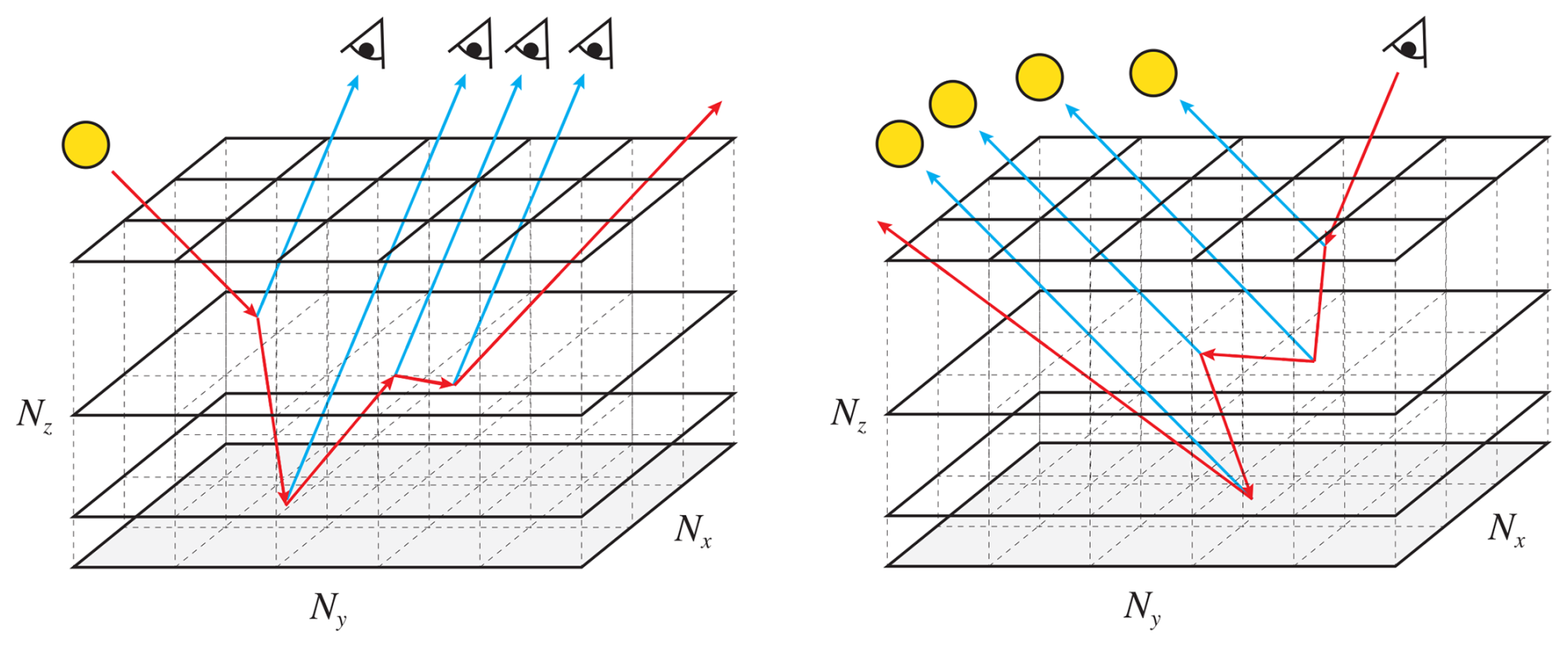
Figure 2 Sketches of the 3D computational domain of MONKI with a photon trajectory (red arrows) in forward mode (left) and backward mode (right). Here, the numbers of columns in the x and y directions are N_x=3 and N_y=5, respectively, while N_z=3 is the number of layers. The domain is periodic in the horizontal directions. At every scattering event (i.e. each change in direction of the red arrow), the probability of scattering towards the detector/eye (in forward mode) or towards the light source/Sun (in backward mode) is computed according to the local estimation method (blue arrows).

To indicate in our Monte Carlo simulations the location and direction of a photon that travels through the computational domain, we use the vectors x and ω, that denote position and propagation direction, respectively:

$$\begin{array}{}\text{(7)}& \mathit{x}=\left[\begin{array}{c}x\\ y\\ z\end{array}\right],\mathit{\omega }=\left[\begin{array}{c}\sin \mathit{\vartheta }\cos \mathit{\phi }\\ \sin \mathit{\vartheta }\sin \mathit{\phi }\\ \cos \mathit{\vartheta }\end{array}\right].\end{array}$$

Here, ϑ and φ are the local zenith and azimuth angles, respectively, as defined in Sect. 2.1 and shown in Fig. 1. Throughout the description of the method, ω denotes a generic photon propagation direction. At a scattering event, we use ω^′ for the propagation direction of the photon incident on the scattering particle, and ω for the propagation direction after scattering, consistent with the angular notation in Fig. 1.

The light source (the Sun) and the observer (the detector) are assumed to be sufficiently far from the computational domain that the incident solar beam and the rays towards the detector can be treated as collimated. We denote the entry point of a photon of the incident sunlight at TOA by x₀, and its direction of propagation by ω₀. Similarly, x^• denotes the point where a photon travelling in the detector direction intersects the TOA or BOA boundary, and ω^• denotes the propagation direction of light towards the detector. The directions ω₀ and ω^• are therefore constant throughout the domain. When needed, O denotes the horizontal area of a selected detector grid column at TOA or BOA.

2.3 Calculating the reflected and transmitted sunlight

Given an atmosphere-surface system, MONKI computes the total and polarised radiances reflected at TOA, or transmitted at BOA, using the Monte Carlo method (see, e.g., Marshak and Davis, 2005): photons are traced through the system.² Since MONKI fully accounts for the polarisation of light, a photon is represented by a normalised Stokes vector, $\stackrel{\mathrm{‾}}{\mathit{I}}=[\mathrm{1},\stackrel{\mathrm{‾}}{Q},\stackrel{\mathrm{‾}}{U},\stackrel{\mathrm{‾}}{V}{]}^{\mathrm{T}}$, carrying a weight, w, that represents the probability of “survival” of the photon (i.e., w will become zero upon total absorption). Since $\stackrel{\mathrm{‾}}{\mathit{I}}$ changes along the photon trajectory, its dependence on position, direction, and previous events is omitted for readability. The trajectory of a photon in the forward mode is summarised in the flow diagram in Fig. 3, which is explained below. We refer to Appendices G1 to G7 for the derivation of the forward Monte Carlo equations for polarised light as used in this section. A similar diagram applies for the backward mode, by replacing “detector” with “the Sun” (see Sect. 2.4).

Figure 3 Flow diagram of a photon trajectory in MONKI in forward mode. The boxes in the grey area pertain to the trajectory of the photon through the atmosphere-surface domain, while the boxes in the blue and green areas represent interactions with the atmosphere and surface, respectively.

At the start of a forward simulation for light with a given wavelength λ, photons are injected at TOA at randomly sampled entry points x₀, with propagation direction ω₀, normalised Stokes vector $\stackrel{\mathrm{‾}}{\mathit{I}}=\mathbf{1}$, and weight w=1. Before a photon moves through the domain, the free photon path length d (the straight geometrical distance travelled until an atmospheric event, i.e. scattering or absorption, occurs) is sampled as follows (see Appendix B):

$$\begin{array}{}\text{(8)}& d={\displaystyle \frac{-\ln \left({\mathit{\xi }}_{\mathrm{1}}\right)}{\mathit{\beta }}},\end{array}$$

where ξ₁ is a random number in the open interval (0,1), drawn from a uniform distribution. Quantity β is the atmospheric extinction coefficient in m⁻¹, which depends on the vertical optical thickness b and the vertical extent Δz of the grid cell via $\mathit{\beta }=b/\mathrm{\Delta }z$. The wavelength dependence and spatial distribution of b across the 3D grid depend on the scattering and absorption optical thicknesses of the gases and aerosol particles in the grid cells (see Appendix A for a description of the model atmosphere). Although all optical properties and radiances generally depend on the wavelength, we omit the λ-notation here. In the current version of MONKI, we only consider elastic scattering processes, that is, for which the wavelength of the light remains invariant.

Next, the free path length d is compared with the distance along the straight photon path to the boundary of the grid cell, to check whether the atmospheric event occurs in the current cell. If so, the photon is moved to the atmospheric event location. If not, the photon is moved along its straight path to the grid cell boundary. The grid cell boundary may be (1) the surface, (2) TOA where the photon leaves the simulation, or (3) the boundary of an adjacent grid cell. In the latter case, the free path length that remains after reaching the boundary is rescaled using the β value of the grid cell that the photon enters.

If an atmospheric event occurs, the photon interacts with one of the atmospheric constituents present in the grid cell: either the gas or one of the N_c aerosol types. To determine which constituent is encountered, we draw a uniformly distributed random number ξ₂ between 0 and 1 and solve the following inequality for the constituent type index t (see, e.g., Eq. 18 of Barker et al., 2003):

$$\begin{array}{}\text{(9)}& \sum _{t^{\prime }=\mathrm{1}}^{t-\mathrm{1}}{\displaystyle \frac{{\mathit{\beta }}_{t^{\prime }}}{\mathit{\beta }}}\le {\mathit{\xi }}_{\mathrm{2}}<\sum _{t^{\prime }=\mathrm{1}}^t{\displaystyle \frac{{\mathit{\beta }}_{t^{\prime }}}{\mathit{\beta }}},\end{array}$$

where ${\mathit{\beta }}_{t^{\prime }}$ is the total extinction coefficient of constituent t^′ in the grid cell. Here, the constituents comprise the gas and the N_c aerosol types, and $\mathit{\beta }={\sum }_{t^{\prime }}{\mathit{\beta }}_{t^{\prime }}$ is the total extinction coefficient of the grid cell. Appendix A explains how this constituent-wise treatment is related to the effective optical properties of a grid cell that contains gas molecules and one or more aerosol types.

In an atmospheric event, the photon is either absorbed or scattered by the constituent that it encounters. The probability of scattering is, by definition, equal to the single-scattering albedo a_t of that constituent, and that of absorption equals (1−a_t). Instead of removing the photon from the simulation upon absorption, we apply a more efficient approach: multiplying the photon weight w by a_t. Thus, if the gas is selected, w is multiplied by a^m; if aerosol type c is selected, w is multiplied by $a_c^{\mathrm{a}}$ (see Appendix A). If the photon has lost virtually all of its weight³, the photon is removed from the simulation. Otherwise, its contribution to the TOA or BOA signal measured by the detector for this scattering event is computed, as explained below.

Instead of collecting photons within the narrow solid angle subtended by the detector, MONKI uses the more efficient “local estimation method” (Marchuk et al., 1980; Marshak and Davis, 2005), a standard approach in Monte Carlo radiative transfer algorithms (see, e.g., Spada et al., 2006; Mayer, 2009; Deutschmann et al., 2011). In this method, the photon is used to simulate the signal contributions of all atmospheric scattering and surface reflection events along the photon's trajectory. Suppose that we have a detector towards the direction ω^•. For an atmospheric event involving constituent type t, the contribution to the TOA or BOA signal measured by the detector is expressed by the column vector W:

$$\begin{array}{}\text{(10)}& \begin{array}{rl}\mathit{W}\left({\mathit{\omega }}^{•}\right)& =w\cdot {\displaystyle \frac{\mathrm{1}}{\mathrm{4}\mathit{\pi }}}{\mathbf{Z}}_t(\mathit{x},{\mathit{\omega }}^{•},{\mathit{\omega }}^{\prime })\cdot {\stackrel{\mathrm{‾}}{\mathit{I}}}^{\prime }\\ & \cdot \exp \left(-\underset{\mathrm{0}}{\overset{s^{•}}{\int }}\mathit{\beta }(\mathit{x}+s^{\prime }{\mathit{\omega }}^{•})\mathrm{d}{s}^{\prime }\right),\end{array}\end{array}$$

where the exponential term represents the direct transmittance along the straight path s^′ in direction ω^•, from the location x of the considered event ($s^{\prime }=\mathrm{0}$) to the detector boundary ($s^{\prime }=s^{•}$), and ${\mathbf{Z}}_t/\left(\mathrm{4}\mathit{\pi }\right)$ is the normalised 4×4 phase matrix of the selected constituent type, describing the scattering of the event's incident normalised Stokes vector ${\stackrel{\mathrm{‾}}{\mathit{I}}}^{\prime }$ in direction ω^′ towards the detector in direction ω^•. The extinction coefficient β in the transmittance term is the total extinction coefficient of the atmospheric mixture along the path. MONKI can, in practice, compute the result of Eq. (10) simultaneously for multiple viewing zenith angles ϑ^• given a viewing azimuth angle φ^•.

For the selected atmospheric constituent type t, the phase matrix is computed as

$$\begin{array}{}\text{(11)}& {\mathbf{Z}}_t(\mathit{x},{\mathit{\omega }}^{•},{\mathit{\omega }}^{\prime })=\mathbf{L}(-{\mathit{\sigma }}_{\mathrm{2}}){\mathbf{F}}_t(\mathit{x},\mathrm{\Theta })\mathbf{L}(-{\mathit{\sigma }}_{\mathrm{1}}),\end{array}$$

where F_t is the single-scattering matrix of the selected constituent, i.e. the gas or one of the aerosol types at x (see Appendix A). Matrix F_t depends on the scattering angle $\mathrm{\Theta }=\arccos ({\mathit{\omega }}^{•}\cdot {\mathit{\omega }}^{\prime })$ (see Fig. 1) and on λ. Matrix L is the 4 × 4 rotation matrix that transforms the Stokes vector between different reference planes (see Hovenier and van der Mee, 1983):

$$\begin{array}{}\text{(12)}& \mathbf{L}\left(\mathit{\alpha }\right)=\left(\begin{array}{cccc}\mathrm{1}& \mathrm{0}& \mathrm{0}& \mathrm{0}\\ \mathrm{0}& \cos \mathrm{2}\mathit{\alpha }& \sin \mathrm{2}\mathit{\alpha }& \mathrm{0}\\ \mathrm{0}& -\sin \mathrm{2}\mathit{\alpha }& \cos \mathrm{2}\mathit{\alpha }& \mathrm{0}\\ \mathrm{0}& \mathrm{0}& \mathrm{0}& \mathrm{1}\end{array}\right).\end{array}$$

Rotation angle α is positive in the anti-clockwise direction when viewed along the propagation direction of the light. Specifically, angles −σ₁ and −σ₂ in Eq. (11) are the angles required to rotate the reference plane from the local meridian plane of the incident beam to the local meridian plane of the scattered beam (see Fig. 1). For a given incident photon direction and selected atmospheric constituent, matrix Z_t thus generally depends on the two angles that describe the detector direction ω^•, namely ϑ^• and φ^•.

If the photon reaches the surface, w is multiplied by the surface albedo, A_s, which equals the probability of reflection by the Lambertian surface. The value of A_s can depend on λ. If the photon retains enough weight (see footnote 3) and the detector is at TOA, the surface reflection contribution to the TOA signal is computed, again using Eq. (10). For A_s>0, the atmospheric scattering factor ${\mathbf{Z}}_t/\left(\mathrm{4}\mathit{\pi }\right)$ in Eq. (10) is replaced by:

$$\begin{array}{}\text{(13)}& {\displaystyle \frac{{\mathit{\mu }}_{•}}{\mathit{\pi }}}{\displaystyle \frac{\mathrm{1}}{A_{\mathrm{s}}}}{\mathbf{R}}_{\mathrm{L}}=\left(\begin{array}{cccc}{\mathit{\mu }}_{•}/\mathit{\pi }& \mathrm{0}& \mathrm{0}& \mathrm{0}\\ \mathrm{0}& \mathrm{0}& \mathrm{0}& \mathrm{0}\\ \mathrm{0}& \mathrm{0}& \mathrm{0}& \mathrm{0}\\ \mathrm{0}& \mathrm{0}& \mathrm{0}& \mathrm{0}\end{array}\right),\end{array}$$

where ${\mathit{\mu }}_{•}=\left|\cos {\mathit{\vartheta }}^{•}\right|$, with ϑ^• the zenith angle corresponding to the detector direction ω^•. The factor ${\mathit{\mu }}_{•}/\mathit{\pi }$ corresponds to the probability density function of the Lambertian surface reflection direction (see Eq. C3), and R_L is the 4×4 Lambertian surface reflection matrix, which is filled with zeros except for its upper left element which equals A_s (see Eq. 13). The division by A_s is necessary because, as explained above, the multiplication by A_s is already included in w.

After computing the event's contribution to the TOA or BOA signal, the new propagation direction of the photon, ω, is sampled from the probability density function of the atmospheric scattering or surface reflection direction. To sample this new direction, we apply either the inverse transform method or the acceptance-rejection method, depending on the type of event, fully accounting for the photon's state of polarisation along its trajectory (see Appendices C, D, E, and F for details on those methods and the choice of method). For the continuation of the photon's trajectory after an atmospheric event, its Stokes vector is adjusted as follows (see Appendix G7):

$$\begin{array}{}\text{(14)}& \stackrel{\mathrm{‾}}{\mathit{I}}={\displaystyle \frac{{\mathbf{Z}}_t(\mathit{x},\mathit{\omega },{\mathit{\omega }}^{\prime }){\stackrel{\mathrm{‾}}{\mathit{I}}}^{\prime }}{{\left[{\mathbf{Z}}_t(\mathit{x},\mathit{\omega },{\mathit{\omega }}^{\prime }){\stackrel{\mathrm{‾}}{\mathit{I}}}^{\prime }\right]}_{\mathrm{1}}}},\end{array}$$

where ${\stackrel{\mathrm{‾}}{\mathit{I}}}^{\prime }$ is the normalised Stokes vector before the event, and Z_t is computed for the newly sampled propagation direction ω and the incident direction ω^′. The division by the first element, indicated by […]₁, of the scattered Stokes vector is necessary for normalisation. Indeed, in this way the first element of $\stackrel{\mathrm{‾}}{\mathit{I}}$ remains equal to 1.0, as the directional dependence of I is already taken care of in the sampling of the new photon direction, while the probability of scattering instead of absorption at an atmospheric event is captured by w. For a surface event, we set $\stackrel{\mathrm{‾}}{\mathit{I}}=\mathbf{1}$, because the Lambertian reflection fully depolarises the photon, while the probability of surface reflection instead of absorption is captured by the multiplication of w by A_s.

Next, a new free path length d is sampled using Eq. (8) in case of an atmospheric event, or the remaining free path length is computed in case of a surface event. The photon continues its trajectory, where it again may be (partially) absorbed or scattered, or reflected by the surface.

Finally, the detector radiance Stokes vector in the direction ω^• and at wavelength λ, for a given grid column and averaged over its horizontal area O at TOA or BOA, is computed using the unbiased estimator (see also Appendix G10):

$$\begin{array}{}\text{(15)}& \begin{array}{rl}& \mathit{I}(O,{\mathit{\omega }}^{•};{\mathit{\omega }}_{\mathrm{0}})\approx {\displaystyle \frac{{\mathit{\mu }}_{\mathrm{0}}}{{\mathit{\mu }}_{•}}}{\displaystyle \frac{E_{\mathrm{0}}}{N}}\sum _{j=\mathrm{1}}^{N_x{N}_y}\sum _{i=\mathrm{1}}^N\sum _{n=\mathrm{1}}^{M_{i,j}}{\mathit{W}}_{n,i,j}{\mathit{\chi }}_{n,i,j},\\ & \mathrm{where}{\mathit{\chi }}_{n,i,j}=\left\{\begin{array}{ll}\mathrm{1},& \text{if }{\mathit{x}}_{n,i,j}^{•}\in O,\\ \mathrm{0},& \text{otherwise.}\end{array}\right.\end{array}\end{array}$$

The summation is performed over all M_i,j scattering and surface reflection events of all N photons injected into each of the N_x×N_y grid columns at TOA. By default, MONKI assumes E₀=π. Vector ${\mathit{W}}_{n,i,j}$ denotes the local-estimation contribution of event n of photon i injected in source column j towards the detector direction ω^• (Eq. 10), and the indicator function ${\mathit{\chi }}_{n,i,j}$ selects only those contributions whose straight detector path intersects TOA or BOA within the horizontal area O of the considered grid column, at location ${\mathit{x}}_{n,i,j}^{•}$. Thus, photons injected in grid columns other than the considered one can also contribute to its signal. The factor ${\mathit{\mu }}_{\mathrm{0}}/{\mathit{\mu }}_{•}$ accounts for the conversion between the horizontal source and detector areas associated with the same scattering volume element (see Appendix G6). The explicit dependence of I on the horizontal area O is only relevant for horizontally inhomogeneous scenes, where the estimator yields the radiance Stokes vector averaged over that area. For horizontally homogeneous scenes, this dependence vanishes because the same radiance is obtained everywhere within O.

2.4 Backward Monte Carlo simulation

MONKI can be used in both forward and backward modes. In backward mode, photon paths are traced from the detector towards the light source (the Sun), as illustrated in Fig. 2. The detector radiance Stokes vector is again computed using the local estimation method, here with the option to evaluate multiple solar zenith angles ϑ₀ at a fixed solar azimuth angle φ₀ simultaneously.

The backward mode is particularly useful when the detector is at a finite distance from, or even inside, the atmosphere-surface system. Although this application is not treated in the present paper, it is important for future extensions of MONKI to spherical atmospheres in combination with a detector at a finite distance. In such cases, the path from a scattering event to the detector depends on the location of the event, and the detector cannot be represented by a single collimated viewing direction throughout the domain. Consequently, in forward mode, only a small fraction of photons launched from the source would reach the detector's field of view, severely limiting the code's efficiency. In backward mode, by contrast, photons are launched from the detector, so that all traced photon paths lie within its field of view. Assuming collimated illumination from a light source at infinite distance, every backward-traced photon that is not completely absorbed can, in principle, be connected to the source direction and therefore contributes to the local estimate. We refer to Appendix G8 for the derivation of the backward Monte Carlo equations for polarised light as used in this section.

According to the reciprocity principle (see Sect. 2.4 of Hovenier et al., 2004), reversing a light path through a medium preserves the reflectance and transmittance along the original path. In practice, this principle allows swapping the light source and detector in a radiative transfer simulation and launching photons in the reverse direction. In the following, we continue to use ω^′ and ω for the incident and scattered propagation directions in the associated forward trajectory. Thus, along the backward trajectory, the photon arrives at the current event from the detector side with propagation direction −ω, and leaves the event towards the source side with propagation direction $-{\mathit{\omega }}^{\prime }$. Reversing both propagation directions leaves the scattering angle $\mathrm{\Theta }=\arccos \left(\right(-\mathit{\omega })\cdot (-{\mathit{\omega }}^{\prime }\left)\right)=\arccos (\mathit{\omega }\cdot {\mathit{\omega }}^{\prime })$ unchanged.

At atmospheric events in the backward mode, the interacting constituent type t is selected in the same way as in the forward mode, and the photon weight is multiplied by the corresponding single-scattering albedo a_t. Because MONKI accounts for polarisation, the orientation of the Stokes vector must be mirrored relative to the reference plane when tracing the reversed photon trajectory. That is, the phase matrices used in the reversed light path do not give the desired result (which is the scattered radiance in the forward light path), and must be corrected as follows (see Eq. 3.37 of Hovenier et al., 2004)⁴:

$$\begin{array}{}\text{(16)}& {\mathbf{Z}}_t(\mathit{x},\mathit{\omega },{\mathit{\omega }}^{\prime })={\mathbf{\Delta }}_{\mathrm{3}}{\mathbf{Z}}_t(\mathit{x},-{\mathit{\omega }}^{\prime },-\mathit{\omega }{)}^{\mathrm{T}}{\mathbf{\Delta }}_{\mathrm{3}},\end{array}$$

where the minus signs indicate reversed propagation directions, the superscript T denotes the transpose, and Δ₃ is given by

$$\begin{array}{}\text{(17)}& {\mathbf{\Delta }}_{\mathrm{3}}=\left(\begin{array}{cccc}\mathrm{1}& \mathrm{0}& \mathrm{0}& \mathrm{0}\\ \mathrm{0}& \mathrm{1}& \mathrm{0}& \mathrm{0}\\ \mathrm{0}& \mathrm{0}& -\mathrm{1}& \mathrm{0}\\ \mathrm{0}& \mathrm{0}& \mathrm{0}& \mathrm{1}\end{array}\right).\end{array}$$

In the backward mode, the normalised unpolarised incident Stokes vector, $\mathbf{1}=[\mathrm{1},\mathrm{0},\mathrm{0},\mathrm{0}{]}^{\mathrm{T}}$, must be multiplied by the phase matrices at the end of the photon trajectory. That is, the event's contribution to the TOA or BOA signal measured by the detector is computed as follows:

$$\begin{array}{}\text{(18)}& \begin{array}{rl}{\mathit{W}}^{\mathrm{bw}}\left({\mathit{\omega }}_{\mathrm{0}}\right)& =w\cdot \stackrel{\mathrm{‾}}{\mathbf{M}}\cdot {\displaystyle \frac{\mathrm{1}}{\mathrm{4}\mathit{\pi }}}{\mathbf{Z}}_t(\mathit{x},{\mathit{\omega }}_{\mathrm{1}},{\mathit{\omega }}_{\mathrm{0}})\cdot \mathbf{1}\\ & \cdot \exp \left(-\underset{\mathrm{0}}{\overset{s_{\mathrm{0}}}{\int }}\mathit{\beta }(\mathit{x}-s^{\prime }{\mathit{\omega }}_{\mathrm{0}})\mathrm{d}{s}^{\prime }\right),\end{array}\end{array}$$

where the direct transmittance is calculated in direction −ω₀ from the event location x ($s^{\prime }=\mathrm{0}$) to the entry location of the solar beam ($s^{\prime }=s_{\mathrm{0}}$). Matrix $\stackrel{\mathrm{‾}}{\mathbf{M}}$ is the 4×4 normalised detector-response matrix, which contains the cumulative polarisation transformation between the current event and the detector, and its path dependence is omitted from the notation. The phase matrix ${\mathbf{Z}}_t(\mathit{x},{\mathit{\omega }}_{\mathrm{1}},{\mathit{\omega }}_{\mathrm{0}})$ in Eq. (18) describes the first scattering event of the associated forward trajectory, from the sunlight direction ω₀ into the direction ω₁. Along the backward trajectory, this same event is encountered in reverse, from −ω₁ towards −ω₀. Therefore the phase matrix is obtained from the reversed one using the reciprocity correction of Eq. (16). For a surface event, the atmospheric phase-matrix factor ${\mathbf{Z}}_t/\left(\mathrm{4}\mathit{\pi }\right)$ is replaced by the corresponding Lambertian surface-reflection factor, analogous to Eq. (13).

After computing the event's contribution to the TOA or BOA signal, the new upstream direction of the backward-traced photon, $-{\mathit{\omega }}^{\prime }$, is sampled from the polarisation-dependent probability density function of the scattering direction, now using the propagated matrix $\stackrel{\mathrm{‾}}{\mathbf{M}}$ (see Appendix G8). At the start of the backward simulation at the detector, $\stackrel{\mathrm{‾}}{\mathbf{M}}$ is initialised as the identity matrix. It is updated at each event to retain the full polarisation history accumulated along the backward photon trajectory as follows (Appendix G8):

$$\begin{array}{}\text{(19)}& {\stackrel{\mathrm{‾}}{\mathbf{M}}}^{\prime }={\displaystyle \frac{\stackrel{\mathrm{‾}}{\mathbf{M}}{\mathbf{Z}}_t(\mathit{x},\mathit{\omega },{\mathit{\omega }}^{\prime })}{{\left[\stackrel{\mathrm{‾}}{\mathbf{M}}{\mathbf{Z}}_t(\mathit{x},\mathit{\omega },{\mathit{\omega }}^{\prime })\mathbf{1}\right]}_{\mathrm{1}}}}.\end{array}$$

Here, −ω is the propagation direction of the backward-traced photon on the detector side of the current event, and ${\stackrel{\mathrm{‾}}{\mathbf{M}}}^{\prime }$ denotes the updated detector-response matrix after sampling the new upstream propagation direction on the source side, $-{\mathit{\omega }}^{\prime }$. Note that the right-multiplications by Z_t in Eq. (19) for all events are applied before the multiplication by 1 in Eq. (18) (see also Collins et al., 1972). For a surface event, the detector-response matrix is updated analogously, using the corresponding Lambertian surface-reflection matrix instead of the atmospheric phase matrix.

Finally, the detector radiance Stokes vector in the direction ω^• and at wavelength λ, for a given grid column and averaged over its horizontal area O at TOA or BOA, is computed by the unbiased estimator (see Appendix G10):

$$\begin{array}{}\text{(20)}& \mathit{I}(O,{\mathit{\omega }}^{•};{\mathit{\omega }}_{\mathrm{0}})\approx {\displaystyle \frac{E_{\mathrm{0}}}{N}}\sum _{i=\mathrm{1}}^N\sum _{n=\mathrm{1}}^{M_i}{\mathit{W}}_{n,i}^{\mathrm{bw}},\end{array}$$

where the summation is performed over all M_i scattering and surface reflection events of all N photons launched uniformly over the horizontal area O of the considered grid column at TOA or BOA, and again E₀=π by default. Here, ${\mathit{W}}_{n,i}^{\mathrm{bw}}$ denotes the backward local-estimation contribution of event n of photon i (Eq. 18). In contrast to the forward mode (Eq. 15), no factor ${\mathit{\mu }}_{\mathrm{0}}/{\mathit{\mu }}_{•}$, no indicator function χ, and no additional sum over the N_x×N_y source columns appear, because in backward mode the estimator is written directly for photons launched from and averaged over the same detector area O of the considered grid column (see Appendix G10).

2.5 Precomputation of optical paths to the detector

The extinction coefficient β in Eq. (10) depends on the position s^′ along the straight path between the event location and the detector boundary. Coefficient β may vary across grid cells within the 3D domain. Moreover, the lengths of the different path segments within each grid cell depend on both the location of the event and the detector direction ω^•. The integral in Eq. (10) can be numerically evaluated by propagating the photon from the event location to the detector boundary, obtaining β and the path segment length for each grid cell.

This evaluation is computationally expensive, as it must be performed for all events of each photon and every viewing zenith angle of the detector. However, if the path to the detector passes through atmospheric grid cells that have the same optical properties in the horizontal directions, the horizontal cell boundaries can be neglected along this path, as only the extinction coefficient β and the path segment length per layer are relevant. If the event occurs at the bottom boundary of a layer, while the detector is above TOA, then Eq. (10) simplifies to:

$$\begin{array}{}\text{(21)}& \begin{array}{rl}\mathit{W}\left({\mathit{\omega }}^{•}\right)& =w\cdot {\displaystyle \frac{\mathrm{1}}{\mathrm{4}\mathit{\pi }}}{\mathbf{Z}}_t(\mathit{x},{\mathit{\omega }}^{•},{\mathit{\omega }}^{\prime })\cdot {\stackrel{\mathrm{‾}}{\mathit{I}}}^{\prime }\\ & \cdot \exp \left(-{\displaystyle \frac{\mathrm{1}}{{\mathit{\mu }}_{•}}}\sum _{k=k^{*}}^{N_z}{\mathit{\beta }}_k\mathrm{\Delta }{z}_k\right),\end{array}\end{array}$$

where k^* denotes the index of the layer where the event happens and $\mathrm{\Delta }{z}_k/{\mathit{\mu }}_{•}$ is the path segment length through layer k in the direction from the event to the detector. Note that $\frac{\mathrm{1}}{{\mathit{\mu }}_{•}}{\sum }_{k=k^{*}}^{N_z}{\mathit{\beta }}_k\mathrm{\Delta }{z}_k$ can be computed for each k^* and μ_• prior to simulating the photon trajectories. If the event occurs within the atmosphere and not exactly at a layer boundary (as is most often the case), the photon is first propagated by a distance Δs towards the detector until it reaches the nearest layer boundary. The term ${\mathit{\beta }}_{k^{*}}\mathrm{\Delta }s$ is then added to $\frac{\mathrm{1}}{{\mathit{\mu }}_{•}}{\sum }_{k=k^{*}+\mathrm{1}}^{N_z}{\mathit{\beta }}_k\mathrm{\Delta }{z}_k$. A similar approach applies for a detector below BOA. An analogous expression can be derived for the backward mode, by precomputing the optical path from the event towards the sunlight-entry boundary.

In 3D cloudy scenes, there are still many cloud-free paths between atmospheric or surface events and the detector, for example, when events occur in atmospheric layers above the clouds or between patchy clouds. For every grid cell, we precompute whether straight paths to the detector are cloud- and aerosol-free from all cell corners as well as for several points within each cell. If these paths pass through gas only, the grid cell is flagged. Assuming that the gas is horizontally homogeneous, we use Eq. (21) for events in the flagged cells, eliminating the need to propagate photons between the event locations and the detector boundary. This approach is computationally more efficient compared to evaluating Eq. (10), while its results are identical.⁵

2.6 Simulation rounds and noise estimation

The computation of the detector radiance Stokes vector with Eq. (15), or Eq. (20) in backward mode, using N photons per column is called one simulation round. In practice, we perform N_r independent rounds, so that in total N_rN photons per column are used. Let I_r denote the estimate of the first Stokes component obtained in round r. The value reported in this paper is the mean over all rounds,

$$\begin{array}{}\text{(22)}& \langle I\rangle ={\displaystyle \frac{\mathrm{1}}{N_r}}\sum _{r=\mathrm{1}}^{N_r}{I}_r.\end{array}$$

The Monte Carlo noise of this reported mean is estimated from the scatter between the independent round estimates:

$$\begin{array}{}\text{(23)}& {\mathit{\sigma }}_{\langle I\rangle }=\sqrt{{\displaystyle \frac{\mathrm{1}}{N_r-\mathrm{1}}}\left[{\displaystyle \frac{\mathrm{1}}{N_r}}\sum _{r=\mathrm{1}}^{N_r}{I}_r^{\mathrm{2}}-{\left({\displaystyle \frac{\mathrm{1}}{N_r}}\sum _{r=\mathrm{1}}^{N_r}{I}_r\right)}^{\mathrm{2}}\right]}.\end{array}$$

This quantity estimates the standard error of the mean 〈I〉, not the standard deviation of the individual round estimates I_r.⁶ To obtain a reliable estimate of σ_〈I〉, we require N_r≥30. In this paper, we use N_r=100. The same procedure is applied to the other Stokes components Q, U, and V.

3 Validation results

In this section, we present the validation of MONKI. In Sect. 3.1, we validate MONKI's total and polarised radiances for horizontally homogeneous scenes by comparing them with results from the widely used doubling–adding method. In Sect. 3.2, we validate MONKI's total and polarised radiances against benchmark results for thick Rayleigh-scattering atmospheres. In Sect. 3.3, we validate MONKI for scenes with 3D cloud structures. In what follows, all results that we present are for a detector at TOA or BOA. Therefore, we omit the • notation for the detector direction, and use ϑ, φ and μ instead of ϑ^•, φ^• and μ_•.

3.1 Comparison with de Haan et al. (1987)

Here, we present a comparison of total and polarised radiances that emerge from a horizontally homogeneous atmosphere-surface system (i.e., $N_x=N_y=\mathrm{1}$) with the benchmark results of de Haan et al. (1987), who used an efficient doubling-adding algorithm that included full polarisation for all orders of scattering.

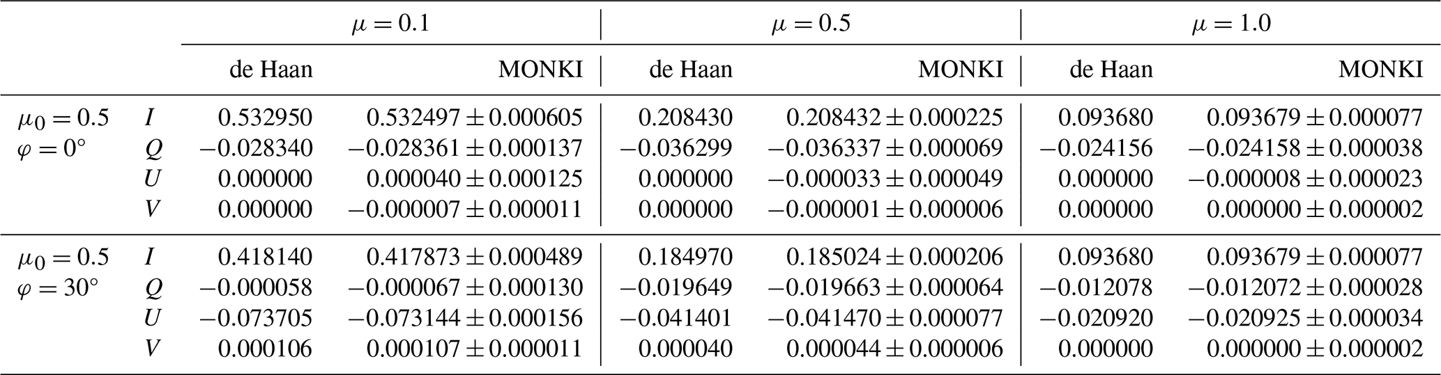
Table 1 Comparison of the TOA radiances computed with MONKI, using 10⁷ photons in forward mode, with the benchmark results of de Haan et al. (1987) for an atmosphere consisting of two plane-parallel layers with a total optical thickness b=0.6 (see text), and an underlying Lambertian reflecting surface with A_s=0.1. The direction of the incident unpolarised light beam is $({\mathit{\mu }}_{\mathrm{0}},{\mathit{\phi }}_{\mathrm{0}})=(\mathrm{0.5},\mathrm{0.0})$. The reported uncertainties in the MONKI results refer to twice the standard error of the mean, evaluated separately for each Stokes component using Eq. (23).

The paper by de Haan et al. (1987) lists benchmark results for different atmosphere-surface systems. We compare with their results for an atmosphere with a total optical thickness b=0.6 that consists of two plane-parallel layers. Both layers contain gaseous molecules with a scattering optical thickness $b_{\mathrm{sca}}^{\mathrm{m}}=\mathrm{0.1}$. The bottom layer also contains water-haze L aerosols (Deirmendjian, 1969), with a scattering optical thickness $b_{\mathrm{sca}}^{\mathrm{a}}=\mathrm{0.4}$. The aerosol characteristics and expansion coefficients at λ=0.70 µm are provided by de Rooij and van der Stap (1984). There is no absorption of light ($b_{\mathrm{abs}}^{\mathrm{m}}=b_{\mathrm{abs}}^{\mathrm{a}}=\mathrm{0}$), and the depolarisation factor of the gaseous molecules is 0.0279, a typical value for terrestrial air. The atmosphere is illuminated from above by unidirectional, unpolarised light propagating in the direction $({\mathit{\mu }}_{\mathrm{0}},{\mathit{\phi }}_{\mathrm{0}})=(\mathrm{0.5},\mathrm{0}\mathit{°})$ with a total flux E₀ equal to π. The Lambertian reflecting surface has an albedo A_s of 0.1.

Table 1 shows the benchmark results and simulated TOA radiances with MONKI for six viewing geometries: $\mathit{\mu }=\mathit{\{}\mathrm{0.1},\mathrm{0.5},\mathrm{1.0}\mathit{\}}$ and $\mathit{\phi }=\mathit{\{}\mathrm{0}\mathit{°},\mathrm{30}\mathit{°}\mathit{\}}$ (see Table 9 of de Haan et al., 1987). The simulations were done in forward mode and used 10⁷ photons in total, distributed over 100 rounds. The listed errors represent twice the standard error of the mean, evaluated separately for each Stokes component using Eq. (23). The results agree excellently: almost all differences between the MONKI results and those of de Haan et al. (1987) fall within twice the standard error of the mean. The magnitude of these differences is comparable to that reported by MYSTIC for simulations with 10⁷ photons, as shown in Table 2 of Emde et al. (2010), and would further decrease if more photons were used. The MONKI results for a solar geometry with $({\mathit{\mu }}_{\mathrm{0}},{\mathit{\phi }}_{\mathrm{0}})=(\mathrm{0.1},\mathrm{0})$ and those for a detector on the surface (not in Table 1) also show excellent agreement (see Tables S1, S2, and S3 in the Supplement). Using MONKI's backward mode, we find similar results (see Tables S4, S5, S6, and S7).

3.2 Comparison with Natraj and Hovenier (2012)

The model atmospheres used by de Haan et al. (1987) are optically relatively thin. Here, we compare with the benchmark results of Natraj and Hovenier (2012), who reported total and polarised radiances of light that is reflected and transmitted by optically thick Rayleigh-scattering atmospheres, computed using the method of X and Y functions (Chandrasekhar, 1960; Natraj et al., 2009). According to Natraj and Hovenier (2012), their results are accurate up to eight decimal places.

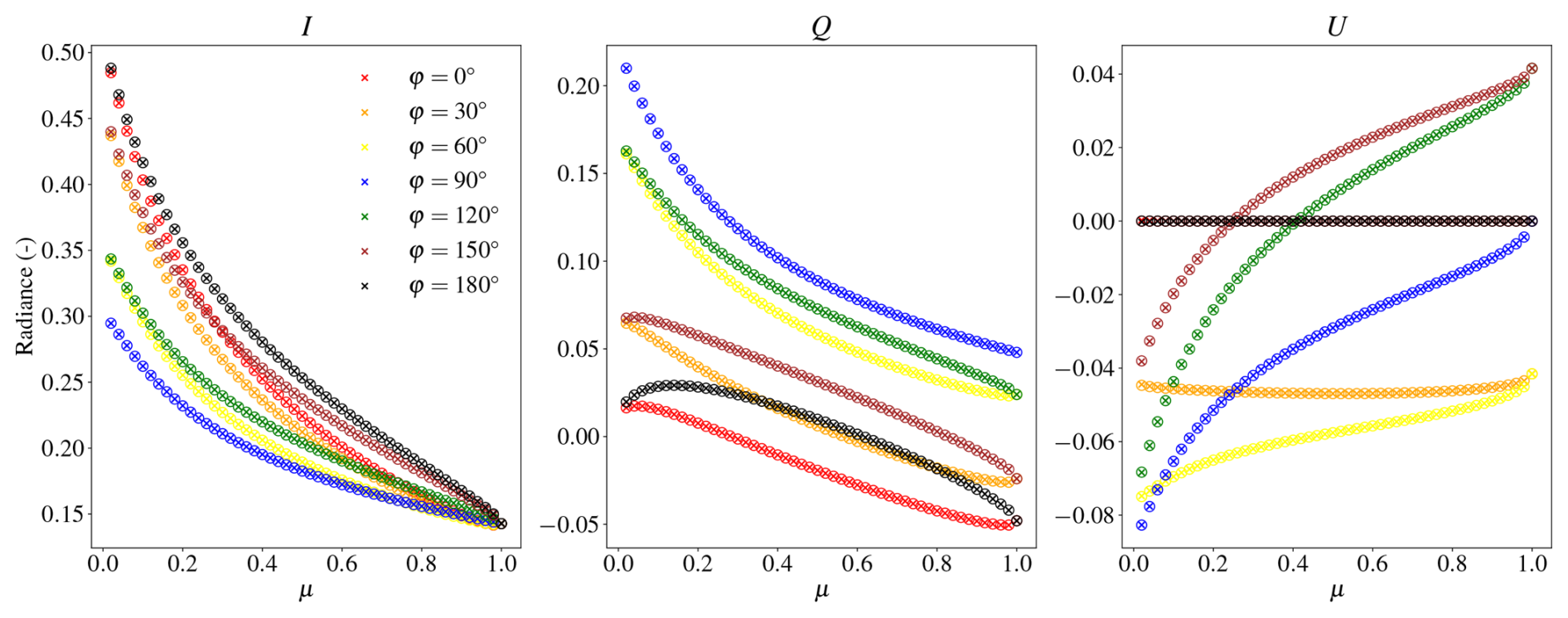
Figure 4 Comparison of the TOA radiances I, Q and U computed with MONKI using 10⁷ photons in forward mode (crosses) with the benchmark results from Natraj and Hovenier (2012) (circles), for a Rayleigh-scattering atmosphere with an optical thickness b=16, a single scattering albedo of 1.0, a depolarisation factor of 0.0, and a black surface below. The different colours indicate different values of φ (φ₀=0°).

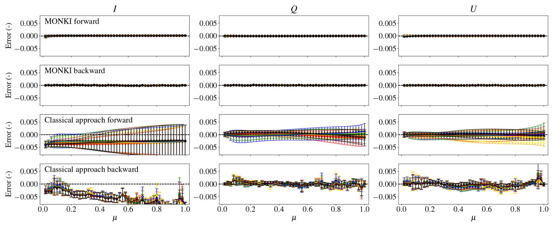
Figure 5 Similar to Fig. 4, but presented as differences (MONKI results minus Natraj and Hovenier results), for MONKI in the forward mode (first row) and in the backward mode (second row), fully taking into account polarisation of light when sampling scattering directions. The third and fourth rows show the results when using instead the classical scattering direction sampling approach in MONKI, as used by, e.g., MYSTIC (see Appendix G9). The error bars indicate the ±2 standard errors of the mean of the simulated results (Eq. 23). Those error bars, and the seven different colours referring to the different values of φ, are virtually indistinguishable for the MONKI forward and backward modes.

We compare to their Tables 1, 3, and 5, which list I, Q and U of light that is reflected by a homogeneous atmospheric layer with an optical thickness b=16. The layer contains only gas, which does not absorb and which has a depolarisation factor of zero. The surface below the layer is black. The atmosphere is illuminated from the top by a beam of unpolarised light with E₀=π, with direction $({\mathit{\mu }}_{\mathrm{0}},{\mathit{\phi }}_{\mathrm{0}})=(\mathrm{0.2},\mathrm{0}\mathit{°})$. Because there is only Rayleigh scattering in the model atmosphere, no circularly polarised light will emerge (see Hansen and Travis, 1974, and Eq. A2), thus V=0 for all geometries. Figure 4 shows I, Q and U computed by MONKI in forward mode using 10⁷ photons distributed over 100 simulation rounds, and as listed by Natraj and Hovenier (2012). Viewing direction μ ranges from 0 to 1.0, and φ from 0 to 180°. As can be seen in Fig. 5, the agreement between the results of MONKI and those of Natraj and Hovenier (2012) is excellent for all geometries, in both forward and backward mode.

MONKI fully accounts for the photon's polarisation history when sampling scattering directions. However, when the classical scattering-direction sampling approach is used in MONKI instead, Fig. 5 (two bottom rows) shows clear deviations and a much larger variance. The classical approach (see Collins et al., 1972) neglects the polarisation state of the incident photon when sampling a new scattering direction, and corrects for this neglect by adjusting the photon's weighting factor (see Appendix G9). Examples of codes that use this approach are MYSTIC (Emde et al., 2010), MSCART (Wang et al., 2017, 2019), SPARTA (Barlakas et al., 2016), IVMCM (Gay et al., 2010), and the backward mode of SMART-G (Ramon et al., 2019). García Muñoz and Mills (2015) pointed out that for thick, strongly polarising⁷ atmospheres, such as those used by Natraj and Hovenier (2012), those codes may fail to converge. This is because, upon multiple scattering, these correction factors are multiplied repeatedly. In the unlikely event that a photon path contains several strongly polarising scattering directions, this can produce infrequent but very large photon weights (see Appendix G9).

Because MONKI fully accounts for the photon's polarisation history it thus does not include such variance-producing corrections (see Appendices D, E, and F). Figure 6 shows MONKI's convergence history when computing the TOA reflectance R₁₁ in both forward and backward modes, for photon numbers up to 10⁷, for μ=1.0, φ=0°, and φ₀=0°, different values of μ₀, and different optical thicknesses b (the single scattering albedo is 1.0). The surface is black. Indeed, for the two cases with μ₀=1.0, namely b=16 and b=4, the lines pertaining to MONKI's forward and backward mode are virtually the same (those cases were also used by García Muñoz and Mills (2015) to demonstrate non-convergence of the classical approach, see their Fig. 8). This was also to be expected, as for this solar and viewing geometry (μ=μ₀), the photon paths in the forward and backward modes are identical. For μ₀=0.5, the photon paths in the forward mode differ from those in the backward mode, and consequently, although MONKI converges to the same values, its convergence history is different for the forward and backward modes. These results show that, unlike classical Monte Carlo codes (right figure in Fig. 6), MONKI converges well for optically thick and polarising atmospheres in both its forward and backward modes.

Figure 6 Left: convergence history of the TOA reflectance, R₁₁, by MONKI in forward mode (solid lines) and backward mode (dotted lines) for a Rayleigh scattering atmosphere with b=4 and μ₀=1.0 (black), b=16 and μ₀=0.5 (blue), and b=16 and μ₀=1.0 (red). The viewing geometry is nadir (μ=1.0). For μ₀=1.0, the solid and dotted lines overlap. Right: similar, but using the classical scattering direction sampling approach in MONKI, as used by, e.g., MYSTIC (see Appendix G9). The jumps are caused by infrequent but large photon weights.

3.3 Comparison with Emde et al. (2018)

In the previous sections, we validated MONKI for horizontally homogeneous atmosphere-surface systems. Here, we validate MONKI for horizontally inhomogeneous (3D) cloudy atmospheres by comparing with benchmarks from the polarised radiative transfer model intercomparison project (IPRT) (Emde et al., 2018).

Figure 7 MONKI results (columns 1 and 2) of the radiance I divided by E₀ (top row) and degree of polarisation P in % (bottom row), for a cubic cloud inside a Rayleigh scattering atmosphere, and the differences between the MONKI results and those of MYSTIC (columns 3 and 4). Results are shown for 2 of the 9 cases described by Emde et al. (2018). In case 4 (columns 1 and 3), the detector is on the surface (BOA), and in case 9 (columns 2 and 4), the detector is at TOA. The sunlight is incident from left to right along the x-direction. The solar and viewing angles are given in Table S8. Because of the horizontal periodicity, the cloud shadow crosses the right domain boundary and re-enters the domain on the left-hand side.

Our first comparison with IPRT results is for a homogeneous Rayleigh scattering atmosphere with b=0.5, that has a cubic-shaped cloud with an optical thickness of 10 embedded (see Sect. 5 of Emde et al., 2018). The single scattering albedo of the gaseous molecules is 1.0 and the depolarisation factor is 0.0. The cloud droplets are spherical with their sizes described by a gamma distribution with effective radii of 10 µm and an effective variance of 0.1. Their single scattering albedo is 1.0. We use their single scattering matrices at λ=800 nm as provided by the IPRT. The surface reflects Lambertian with an albedo of 0.2.

The cloud has dimensions of 1 × 1 × 1 km³, and extends from 2 to 3 km altitude. The computational domain extends to an altitude of 5 km. Horizontally, the domain spans 7 km in both directions, with periodic boundary conditions. Both the light source and the detector are at infinite distances from the atmosphere-surface system: the solar and viewing geometries are the same across the domain. The horizontal area of 7×7 km² is covered by 70×70 pixels. MONKI used 10⁷ photons per pixel, matching the number of photons used in the IPRT (Emde et al., 2018).

Figure 7 shows the results of MONKI (in forward mode) for the radiance I and degree of polarisation P, for IPRT-cases 4 and 9, that differ in solar and viewing geometries (see Table 4 of Emde et al., 2018). Because MONKI defines the angles slightly differently from Emde et al. (2018), we have listed the geometries in Table S8 in the Supplement. Figure S1 in the Supplement shows the results for all 9 cases and all Stokes parameters, with cases 1 to 4 pertaining to light transmitted through the atmosphere, thus at BOA, and cases 5 to 9 pertaining to reflected light, thus at TOA. Results for cases 1 to 4 are stored on the x,y-grid at the surface, whereas results for cases 5 to 9 are stored on the x,y-grid at TOA.⁸

The radiance I in the cloud-free regions of cases 1 to 4 (BOA) is smaller than in cases 5 to 9 (TOA), due to the larger contribution of the surface reflection in the latter cases (see Fig. S1). Cases 5 to 9 (TOA) show shadows on the surface, while cases 1 to 4 (BOA) only show subtle shadows in the sky. Note that due to horizontal periodicity, the shadow of the cloud stretches outside the right-hand side of the domain and back into the domain on the left-hand side. The difference between the surface and sky shadows is, for instance, evident in P for case 9 (see Fig. S1), where P on the right-hand side of the cloud is relatively low due to the atmospheric shadow: in this part of the atmosphere, the direct sunlight is attenuated by the cloud. Instead, this part of the atmosphere is mostly illuminated by diffuse light with generally a lower degree of polarisation due to randomisation (see Fig. 7 of Trees et al., 2025). Above the cloud shadow on the surface, P is high because the shadow suppresses the unpolarised contribution of light that has been reflected by the Lambertian surface. For a detailed discussion of the features in Figs. 7 and S1, see Sect. 5 of Emde et al. (2018).

MONKI's results closely match the benchmark results (cf. Fig. A2 of Emde et al., 2018). Figure 7 shows the differences between MONKI and MYSTIC for test cases 4 and 9 for I and P, and Fig. S2 in the Supplement shows the differences for all nine cases and all Stokes parameters. In the cloud-free regions, the differences in I, Q, U, and V are nearly zero. Small, random differences in P remain below 0.07 % and are centred around zero. In cloudy pixels, the differences are larger, as expected because of increased simulation noise. This effect is common in Monte Carlo codes due to infrequent but significant contributions in the local estimation method associated with strongly forward-peaked Mie scattering phase functions of the cloud droplets (see, e.g., Barker et al., 2003). Nevertheless, these differences remain below 2.82 × 10⁻³, 0.66 × 10⁻³, 0.63 × 10⁻³, 10.98 × 10⁻⁵, and 0.49 % for I, Q, U, V, and P, respectively, and are centred around zero for all cases. Increasing the number of photons would reduce this random noise. We find no systematic biases between MONKI and MYSTIC.

Figure 8 Results of MONKI in forward (“MONKI-F”) and backward mode (“MONKI-B”) for the cubic cloud scenario of Emde et al. (2018), cases 4 (rows 1 and 2) and 9 (rows 3 and 4), for a cross-section through the domain at y=3.95 km (see Fig. S1 in the Supplement). Stokes parameters I, Q, U and V are shown in four columns, also for the other codes in the IPRT project, with the absolute differences of all codes with MYSTIC below. The grey area in the difference plots corresponds to 2 standard deviations of 3DMCPOL. The Stokes parameters are normalised to $\mathrm{1000}/E_{\mathrm{0}}$.

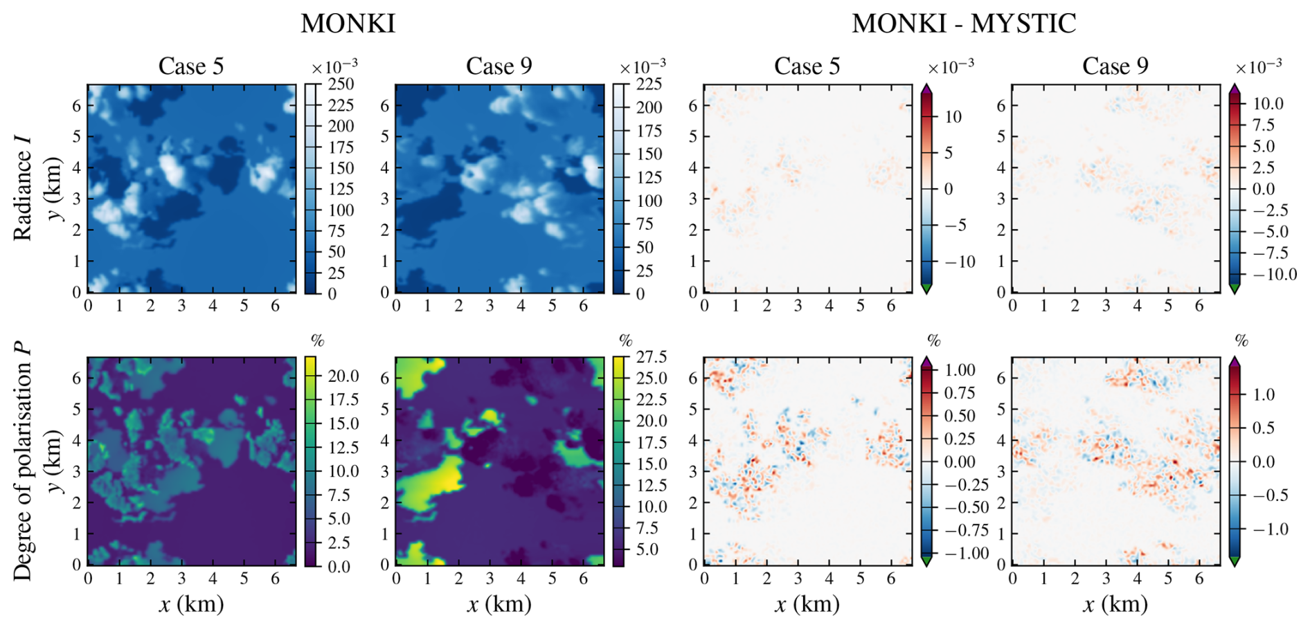
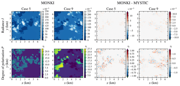
Figure 9 MONKI results (columns 1 and 2) of the radiance I (row 1) and P (row 2), for a 3D cumulus cloud field inside a scattering and absorbing gaseous atmosphere (Emde et al., 2018), for 2 different solar and viewing geometries with a detector at TOA (cases 5 and 9 in Table S8). The sunlight is incident from left to right along the x-direction. Radiance I is divided by E₀, and P is in %. Columns 3 and 4 show the differences between MONKI and MYSTIC.

To demonstrate how MONKI performs compared to other codes, Fig. 8 shows cross-sections at y=3.95 km of the results of MONKI in both forward and backward modes for cases 4 and 9, together with results of the codes used in the IPRT project (Emde et al., 2018). Also, the differences with MYSTIC are shown, together with the ±2 standard deviation range of the 3DMCPOL results. The results for all nine cases are shown in Fig. S5 in the Supplement. Unlike some other codes, MONKI shows excellent agreement with MYSTIC in all cases, in both its forward and backward modes.

Emde et al. (2018) also provide test cases for a more realistic scenario: a 3D cumulus cloud field that has been generated by a Large Eddy Simulation (LES) code (Stevens et al., 1999), embedded within a scattering and absorbing gaseous atmosphere. The domain size is 6.7 × 6.7 × 30 km³. The cloud's optical thickness and droplet effective radius vary across the $\mathrm{100}\times \mathrm{100}\times \mathrm{53}$ grid cells (the 12 top layers are cloud-free). For a detailed description of the model, see Emde et al. (2018). Figure 9 shows I and P as computed with MONKI for the solar and viewing geometries of cases 5 and 9 (see Table S8), along with their differences from MYSTIC benchmark results. We used 10⁶ photons per pixel. Once again, we find no systematic biases. Numerical tests showed that the remaining differences decrease when increasing the number of photons.

4 Sample signals for the Earth and Venus

In this section, we present sample simulations with MONKI of sunlight that is locally reflected by the atmospheres of the Earth and Venus. The model atmospheres are horizontally homogeneous (i.e., $N_x=N_y=\mathrm{1}$), as illustrated in Fig. 10. These simulations demonstrate MONKI's versatility in handling different types of atmospheres, following the formulae provided in Appendix A. Below, we first describe the model setting and then the results. The model settings are also summarised in Table 2.

Figure 10 The model atmosphere-surface systems of the Earth (in blue) and Venus (in orange). From left to right: the pressure profiles, temperature profiles, the ozone volume mixing ratio profile for the Earth, the cloud model for the Earth, the cloud model for Venus. Below the latter two graphs, the surface albedo, A_s, is also given.

Peck and Reeder (1972)Sneep and Ubachs (2005); Wilmouth and Sayres (2020)Bass and Paur (1985)

Table 2 Model settings used in the sample simulations of the Earth and Venus at λ=550 nm.

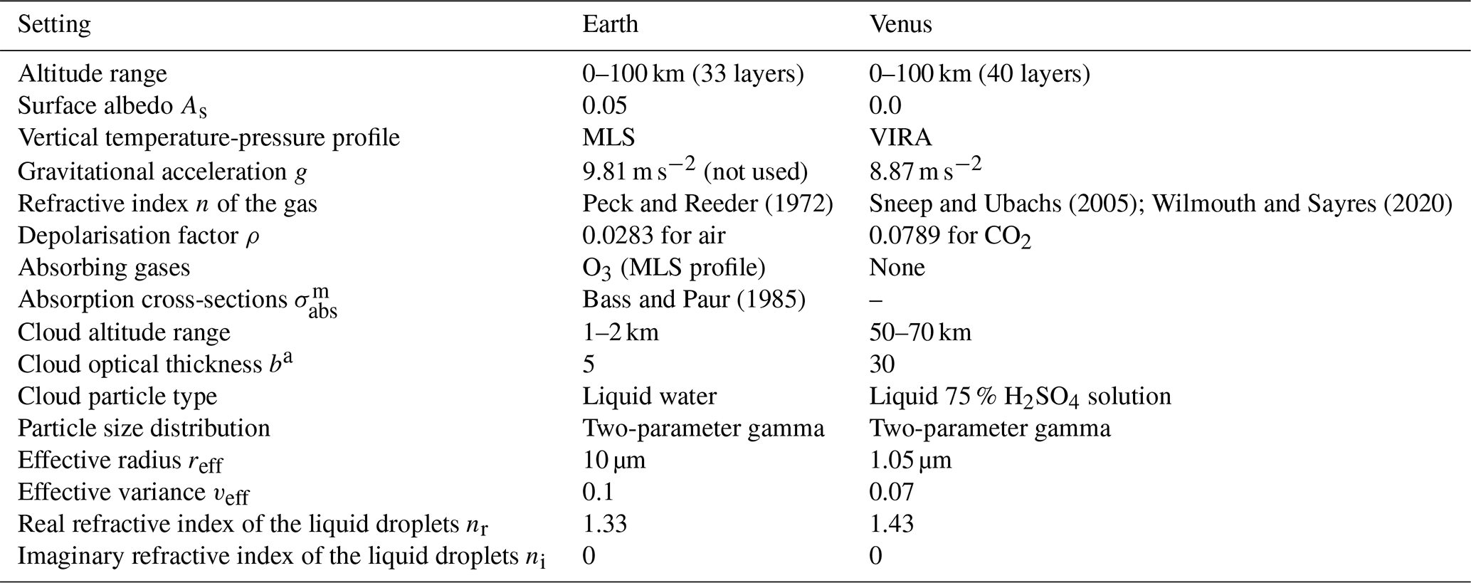
The Earth model atmosphere consists of 33 plane-parallel, horizontally homogeneous layers from 0 to 100 km altitude. The surface reflects Lambertian with an albedo A_s of 0.05. The only absorbing gas is ozone (O₃). The wavelength- and temperature-dependent O₃ absorption cross-sections, ${\mathit{\sigma }}_{\mathrm{abs}}^{\mathrm{m}}(\mathit{\lambda },T)$, are taken from Bass and Paur (1985). Pressure, temperature, and ozone volume mixing ratios (VMRs) vary with altitude according to the standard Mid-Latitude Summer profile (Anderson et al., 1986). We assume that the pressure-to-temperature ratio decreases exponentially with altitude within each layer (see Eq. A10). The refractive index of air, n, is computed with the dispersion formula of Peck and Reeder (1972). The King correction factor F_K of the air (Eq. A9) is the sum of the values for N₂, O₂, Ar, and CO₂ as given by Bates (1984), weighted by the respective mixing ratios of those gases on Earth: 78.084 %, 20.9476 %, 0.934 %, and 0.0375 %. At λ=550 nm, this yields a depolarisation factor ρ=0.0283.

In the Earth scenario, the cloud extends from 1 to 2 km, with a vertically homogeneous optical thickness b^a of 5. We assume a two-parameter gamma distribution for cloud droplet sizes (Hansen and Travis, 1974), with an effective radius r_eff=10 µm and an effective variance v_eff=0.1. The droplets are composed of liquid water with a real refractive index of 1.33 (Hale and Querry, 1973) and an imaginary refractive index of zero (i.e., the single scattering albedo of the cloud droplets is 1.0).

The Venus model atmosphere consists of 40 plane-parallel, horizontally homogeneous layers from 0 to 100 km altitude. At λ=550 nm, the reflected light at TOA is virtually insensitive to Venus's lower atmosphere and surface albedo. Therefore, we use 4 km thick layers from the surface to 40 and 2 km thick layers above 40 km. The surface is assumed black. We neglect gaseous absorption, which is a reasonable assumption for Venus at λ=550 nm (Moroz, 1981; Haus et al., 2015). Pressure profiles follow the Venus International Reference Atmosphere (VIRA) for latitudes up to 30°, based on Seiff et al. (1985), which incorporates data from four Pioneer Venus Probes, the Pioneer Venus Orbiter, and the Venera 10, 12, and 13 landers. We assume hydrostatic equilibrium (Eq. A11), a gravitational acceleration of g=8.87 m s⁻², and the background gas molar mass M is computed by the weighted sum of 96.5 % CO₂ (44.01 g mol⁻¹) and 3.5 % N₂ (28.0134 g mol⁻¹). The values for n and F_K at λ=550 nm are computed with the parametrisations for CO₂ stated in Sneep and Ubachs (2005)⁹, leading to a depolarisation factor ρ=0.0789.

The cloud in the Venus model extends from 50 to 70 km, with a vertically homogeneous optical thickness b^a=30 (see Haus et al., 2015, for more detailed Venus cloud models). The cloud particles are liquid droplets and their properties follow those of Hansen and Hovenier (1974): a two-parameter gamma distribution with an effective radius of 1.05 µm and an effective variance of 0.07. The droplets are composed of 75 % H₂SO₄ solution in water, with a real refractive index of 1.43 at λ=550 nm (Palmer and Williams, 1975). Their single scattering albedo is 1.0.

Figure 11 shows the angular distribution of the singly scattered radiance, F₁₁ (the phase function), and the degree of linear polarisation, $-F_{\mathrm{12}}/F_{\mathrm{11}}$, of the gas and cloud droplets in the Earth and Venus model atmospheres as functions of the scattering angle Θ (see Appendix A for definitions of the single-scattering matrix elements). The large droplets of the Earth cloud produce a strong forward peak in F₁₁ due to diffraction (see Hansen and Travis, 1974). The peaks near Θ=142° and 122° are the primary and secondary cloudbows, caused by, respectively, one and two internal reflections inside the spherical droplets. The radiance and polarisation enhancement near Θ=180° is called the “glory”. These features are less pronounced or absent in the much smaller cloud droplets on Venus. The features due to Rayleigh scattering by gas molecules are similar on Earth and Venus: F₁₁ is fairly isotropic, while polarisation is strongest around Θ=90°. For the Venusian gas, the Rayleigh polarisation maximum is lower than for the Earth's gas because it has a larger depolarisation factor.

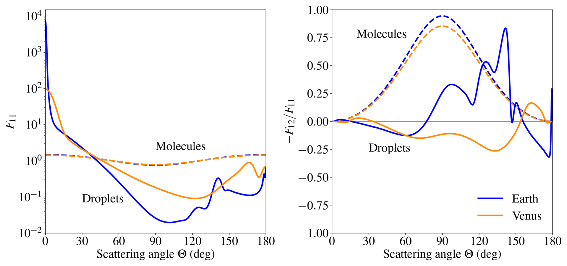
Figure 11 The phase function F₁₁ (left) and the degree of linear polarisation ($-F_{\mathrm{12}}/F_{\mathrm{11}}$) (right) as functions of the scattering angle Θ, for singly scattered light by gaseous molecules (dashed lines) and cloud droplets (solid lines). The blue lines are for Earth-like gas (with a depolarisation factor ρ equal to 0.0283) and cloud particles (r_eff=10 µm), and the orange lines are for Venus-like gas (with ρ=0.0789) and cloud particles (r_eff=1.05 µm). The wavelength of the light is 550 nm.

Figure 12 shows the simulated TOA reflectance, R₁₁, and degree of polarisation, P_s, computed with MONKI for the Earth and Venus model atmosphere–surface systems described above. Simulations were performed for three solar zenith angles: θ₀=0, 45, and 75°. The viewing zenith angles range from θ=0° to θ=89° in 1° increments. The azimuth angle of the sunlight was φ₀=0°. The viewing azimuth angles are φ=0° and 180° (thus U=0). For each combination of the 90 values of θ, and (θ₀,φ), we used 10⁸ photons for the computations for the Earth and 10⁵ photons for Venus (the more isotropic scattering by the small Venusian cloud droplets requires fewer photons). In Fig. S6, we provide the comparison of the computations for the Earth with results computed with Doubling-Adding KNMI (DAK), which uses identical formulae for the optical properties of the model atmosphere as MONKI (see Appendix A).

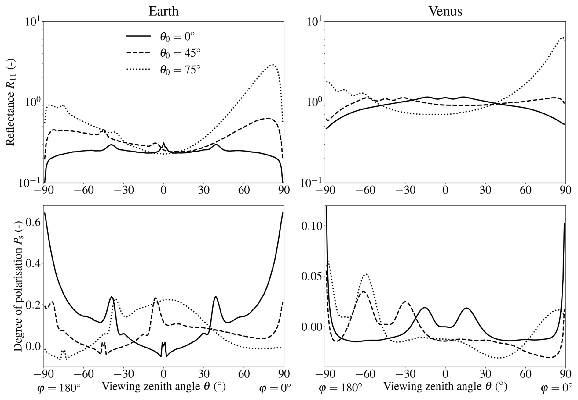
Figure 12 Sample signals of the TOA reflectance R₁₁ (top) and degree of polarisation $P_{\mathrm{s}}=-Q/I$ (bottom), for the Earth (left) and Venus (right), computed with MONKI. Note the different y-scales for P_s. The signals are presented as functions of viewing angle θ, and for solar zenith angles θ₀=0° (solid line), 45° (dashed line), and 75° (dotted line). The azimuth angle of the sunlight φ₀ is 0°.

For the Earth model (Fig. 12), the reflectance R₁₁ generally increases with θ and θ₀. With increasing angles, the optical paths through the gas and clouds increase and multiple scattering increases. Cloud droplet single scattering features (Fig. 11) leave signatures in R₁₁, but show up more distinctly in P_s. The cloudbows emerge near (θ,φ) = (38°,0°), (7°,180°), and (37°,180°), corresponding to the scattering angle Θ=142° for θ₀= 0, 45 and 75°, respectively.¹⁰ The glory shifts from θ=0 to 45 to 75° in the φ=180° direction with increasing θ₀. Rayleigh scattering, which enhances P_s around Θ=90°, causes P_s to peak near θ=90° for θ₀=0° and near (θ,φ) = (10°,0°) for θ₀=75°. This behaviour can be verified with vertical profiles of the layer contributions to the total and polarised TOA reflectances. As an example, Fig. 13 shows those profiles for θ₀=0°, demonstrating that, towards perpendicular scattering geometries, an increasing fraction of the polarised signal originates from the gas above the cloud.

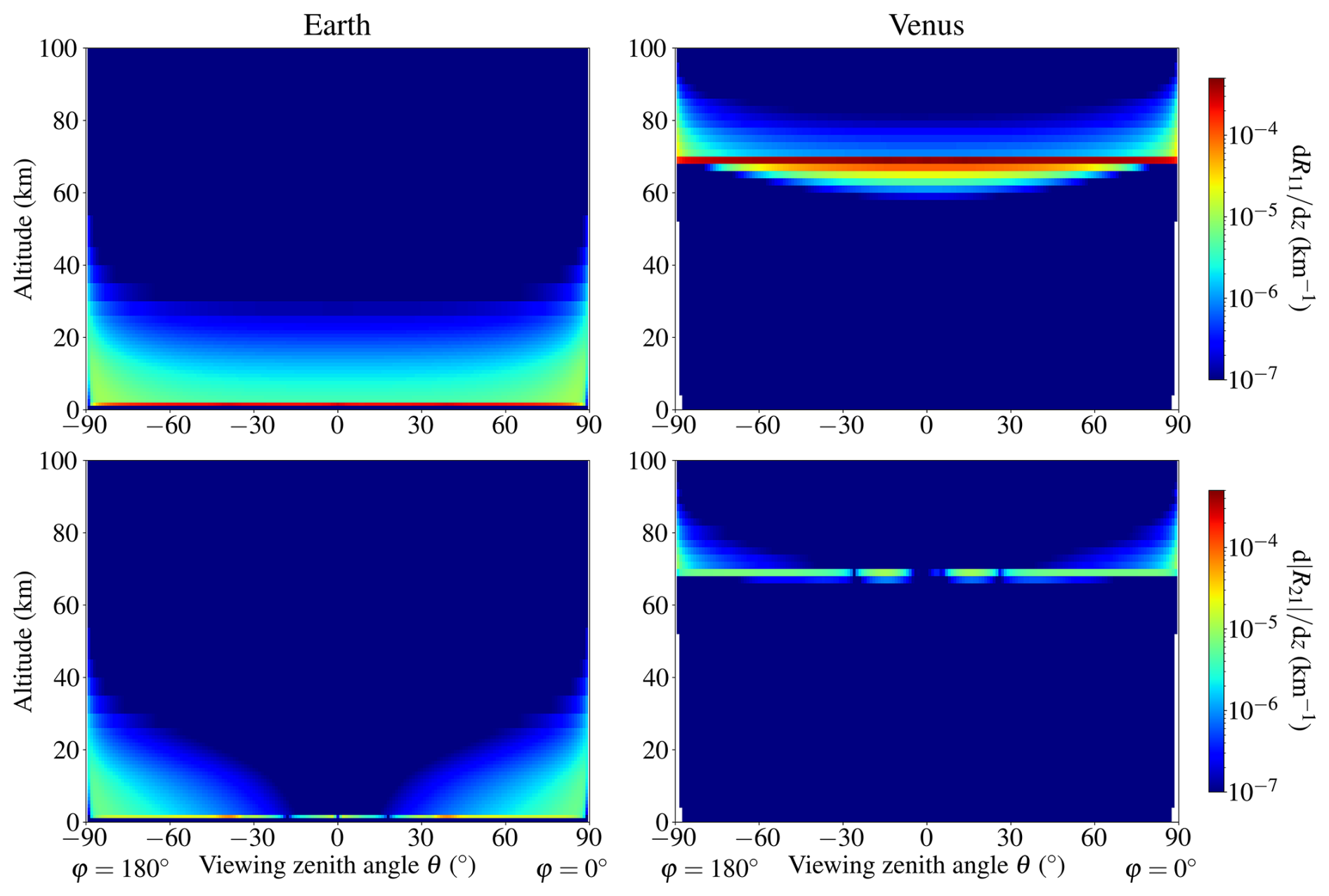
Figure 13 Contributions to the computed TOA reflectances at θ₀=0°, for Earth (left) and Venus (right), plotted as functions of the altitude of the last scattering event of the photons. The contribution profiles are expressed per kilometre (km⁻¹) for the total reflectances R₁₁ (top row) and the polarised reflectances $\left|R_{\mathrm{21}}\right|$ (bottom row).

The Venus results in Fig. 12 show that this planet appears much brighter in locally reflected light than Earth. The higher R₁₁ values are primarily due to the larger cloud optical thickness. As on Earth, cloud droplet single scattering features leave distinct signatures in P_s of the locally reflected light, which can be seen to shift with increasing θ₀, as they are characteristic for given scattering angles. However, the increase in polarisation due to Rayleigh scattering around a scattering angle of 90° is less pronounced on Venus than on Earth. For example, for θ₀=0°, P_s increases only at the largest viewing zenith angles. Despite Venus's large atmospheric pressure at surface level, the cloud deck extends up to 70 km altitude, leaving little gas above the cloud for light to scatter from, as shown in Fig. 13. Instead, the signal is dominated by abundant virtually unpolarised light multiply scattered in the upper parts of the Venusian clouds.

5 Summary, discussion, and outlook

Polarimetry is a powerful tool for characterising planetary atmospheres and surfaces. Radiative transfer simulations of total and polarised radiances are essential for designing, preparing, and operating spectro(polari)metric remote sensing instruments. Even for instruments that do not measure polarisation, accounting for polarisation in simulations is crucial for obtaining accurate total radiance calculations and for assessing potential errors due to an instrument's polarisation sensitivity if no polarisation scrambler is used. With the increasing spatial resolution of current and future Earth observation spectro(polari)meters, simulating 3D radiative transfer effects, such as cloud shadows, becomes increasingly important.

In this paper, we have presented the 3D radiative transfer code MONKI (Monte Carlo KNMI), which fully accounts for the linear and circular polarisation of light at all orders of scattering. MONKI is written in modern Fortran and is based on the Monte Carlo method. Rather than counting photons at the detector, MONKI uses the more efficient “local estimation method”, which calculates the probability of scattering towards the detector at each scattering event. MONKI can compute both horizontally homogeneous and inhomogeneous (3D cloudy) scenes. It can operate both in forward mode (with photons propagating from the source to the detector) and in backward mode (with photons propagating in the opposite direction). Both modes converge to similar results, with comparable computation times in the tested cases.

We compared results of MONKI with benchmark results for polarised radiances in horizontally homogeneous atmospheres (de Haan et al., 1987) and thick Rayleigh-scattering atmospheres (Natraj and Hovenier, 2012). Additionally, we validated MONKI's 3D radiative transfer capabilities using benchmark results for polarised radiances from 3D clouds (Emde et al., 2018). In all cases, MONKI showed excellent agreement with the benchmark results.

Although MONKI is not the first code of its kind, it has fundamental methodological differences from other Monte Carlo codes. A common limitation of Monte Carlo codes is their failure to converge in optically thick and strongly polarising atmospheres. This issue arises when approximations are made in the sampling of scattering directions, by neglecting the photon's polarisation state and correcting afterwards by weight factors. MONKI instead samples scattering directions from the full polarisation-dependent distribution while fully tracking the polarisation history of each photon along its trajectory. As demonstrated in this paper, this exact polarised sampling approach converges in both forward and backward modes, including for optically thick and strongly polarising planetary atmospheres. In addition, the appendices provide a complete derivation of the corresponding forward and backward Monte Carlo equations and polarisation-dependent sampling formulae, thereby offering a unified theoretical framework for polarised Monte Carlo radiative transfer.

The current version of MONKI does not use variance reduction techniques other than the local estimation method. Although such techniques can reduce the noise (and therefore the computation time needed for convergence), they can introduce biases (see, e.g. Barker et al., 2003) and/or increase code complexity. For example, directional importance sampling, which involves adjusting forward-peaked single scattering phase functions and photon weights, and photon splitting (see, e.g. Buras and Mayer, 2011), are mathematically correct but can reduce a code's intuitiveness. By omitting those variance reduction techniques, MONKI produces unbiased results while preserving readability and simplicity, and thus adaptability when future extensions of the code are to be implemented. Instead of using such techniques, we increase the number of photons to achieve higher precision when needed.

In order to speed up MONKI's simulations, we implemented and presented a precomputation approach for optical paths to the detector. By precomputing the optical thickness of the horizontally homogeneous background gas for each atmospheric layer towards the detector, and by identifying grid cells that have cloud- and aerosol-free optical paths to the detector, MONKI avoids repeated photon propagations between the locations of the scattering events and the detector. This approach significantly improves computational efficiency, especially in scenes with low and/or patchy clouds, without compromising the accuracy.

We have presented sample signals of the TOA reflectance and degree of polarisation of light that is locally reflected by the Earth and Venus using horizontally homogeneous cloud models. This exercise demonstrated MONKI's versatility for various atmospheric conditions. For Earth applications, MONKI uses the same method as DAK (Doubling-Adding KNMI) to compute the input atmospheric optical properties. MONKI can handle spectral variations of those properties, producing simulated spectra by so-called line-by-line computations. MONKI can import different particle scattering matrices and can, in principle, also simulate light scattered by non-spherical aerosol particles and ice clouds.

Since MONKI uses the Monte Carlo method, it can store the locations of photon scattering, also for different orders of scattering, for detailed analyses of features in the simulated signals. Among the planned extensions of MONKI is the implementation of atmospheric sphericity, which would allow computations for scenes with a low Sun and/or large viewing angles. We conclude that MONKI is an accurate radiative transfer code, ready to support the design, preparation, and operation of spectro(polari)metric missions for Earth, Venus, and other planets.

Appendix A: Describing the atmosphere and surface

In this appendix, we describe the optical properties of the atmosphere and surface used by MONKI. Each atmospheric grid cell can contain gas molecules and multiple aerosol types, such as cloud or haze particles. For each of these constituents, MONKI uses the total optical thickness, the single-scattering albedo, and the single-scattering matrix.

The total optical thickness of a grid cell is the sum of the optical thicknesses of the gas and all aerosol types:

$$\begin{array}{}\text{(A1)}& \begin{array}{rl}b\left(\mathit{\lambda }\right)& =b^{\mathrm{m}}\left(\mathit{\lambda }\right)+\sum _{c=\mathrm{1}}^{N_c}{b}_c^{\mathrm{a}}\left(\mathit{\lambda }\right)\\ & =b_{\mathrm{sca}}^{\mathrm{m}}\left(\mathit{\lambda }\right)+b_{\mathrm{abs}}^{\mathrm{m}}\left(\mathit{\lambda }\right)+\sum _{c=\mathrm{1}}^{N_c}\left[b_{\mathrm{sca},c}^{\mathrm{a}}\left(\mathit{\lambda }\right)+b_{\mathrm{abs},c}^{\mathrm{a}}\left(\mathit{\lambda }\right)\right],\end{array}\end{array}$$

where superscripts m and a refer to gas molecules and aerosol particles, respectively, and subscripts “sca” and “abs” refer to scattering and absorption. The index $c=\mathrm{1},\mathrm{\dots },N_c$ denotes the aerosol type. For a grid cell with vertical extent Δz, the corresponding total extinction coefficient is $\mathit{\beta }=b/\mathrm{\Delta }z$. Analogous relations hold for the scattering and absorption extinction coefficients, and for each constituent type separately; for example, ${\mathit{\beta }}_t=b_t/\mathrm{\Delta }z$ and ${\mathit{\beta }}_{\mathrm{sca},t}=b_{\mathrm{sca},t}/\mathrm{\Delta }z$ for constituent type t.

A1 Gas molecules

Single scattering of light by gas molecules is described by the anisotropic Rayleigh scattering matrix F^m (Hansen and Travis, 1974):

$$\begin{array}{}\text{(A2)}& {\mathbf{F}}^{\mathrm{m}}(\mathrm{\Theta },\mathit{\lambda })=\left[\begin{array}{cccc}{F}_{\mathrm{11}}^{\mathrm{m}}(\mathrm{\Theta },\mathit{\lambda })& F_{\mathrm{12}}^{\mathrm{m}}(\mathrm{\Theta },\mathit{\lambda })& \mathrm{0}& \mathrm{0}\\ F_{\mathrm{21}}^{\mathrm{m}}(\mathrm{\Theta },\mathit{\lambda })& F_{\mathrm{22}}^{\mathrm{m}}(\mathrm{\Theta },\mathit{\lambda })& \mathrm{0}& \mathrm{0}\\ \mathrm{0}& \mathrm{0}& F_{\mathrm{33}}^{\mathrm{m}}(\mathrm{\Theta },\mathit{\lambda })& \mathrm{0}\\ \mathrm{0}& \mathrm{0}& \mathrm{0}& F_{\mathrm{44}}^{\mathrm{m}}(\mathrm{\Theta },\mathit{\lambda })\end{array}\right].\end{array}$$

Here, Θ is the scattering angle, defined relative to the propagation direction of the incident light, such that Θ=0° corresponds to forward scattering and Θ=180° to backward scattering. The matrix elements are

$$\begin{array}{}\text{(A3)}& {\displaystyle }{F}_{\mathrm{11}}^{\mathrm{m}}(\mathrm{\Theta },\mathit{\lambda })& {\displaystyle }={\displaystyle \frac{\mathrm{3}}{\mathrm{4}}}\mathrm{\Delta }\left(\mathit{\lambda }\right)(\mathrm{1}+{\cos }^{\mathrm{2}}\mathrm{\Theta })+\mathrm{1}-\mathrm{\Delta }\left(\mathit{\lambda }\right),\text{(A4)}& {\displaystyle }{F}_{\mathrm{22}}^{\mathrm{m}}(\mathrm{\Theta },\mathit{\lambda })& {\displaystyle }={\displaystyle \frac{\mathrm{3}}{\mathrm{4}}}\mathrm{\Delta }\left(\mathit{\lambda }\right)(\mathrm{1}+{\cos }^{\mathrm{2}}\mathrm{\Theta }),\text{(A5)}& {\displaystyle }{F}_{\mathrm{33}}^{\mathrm{m}}(\mathrm{\Theta },\mathit{\lambda })& {\displaystyle }={\displaystyle \frac{\mathrm{3}}{\mathrm{2}}}\mathrm{\Delta }\left(\mathit{\lambda }\right)\cos \mathrm{\Theta },\text{(A6)}& {\displaystyle }{F}_{\mathrm{44}}^{\mathrm{m}}(\mathrm{\Theta },\mathit{\lambda })& {\displaystyle }={\displaystyle \frac{\mathrm{3}}{\mathrm{2}}}\mathrm{\Delta }\left(\mathit{\lambda }\right){\mathrm{\Delta }}^{\prime }\left(\mathit{\lambda }\right)\cos \mathrm{\Theta },\text{(A7)}& {\displaystyle }{F}_{\mathrm{12}}^{\mathrm{m}}(\mathrm{\Theta },\mathit{\lambda })& {\displaystyle }=F_{\mathrm{21}}^{\mathrm{m}}(\mathrm{\Theta },\mathit{\lambda })=-{\displaystyle \frac{\mathrm{3}}{\mathrm{4}}}\mathrm{\Delta }\left(\mathit{\lambda }\right){\sin }^{\mathrm{2}}\mathrm{\Theta },\end{array}$$

with

$$\begin{array}{}\text{(A8)}& \mathrm{\Delta }\left(\mathit{\lambda }\right)={\displaystyle \frac{\mathrm{1}-\mathit{\rho }\left(\mathit{\lambda }\right)}{\mathrm{1}+\mathit{\rho }\left(\mathit{\lambda }\right)/\mathrm{2}}},{\mathrm{\Delta }}^{\prime }\left(\mathit{\lambda }\right)={\displaystyle \frac{\mathrm{1}-\mathrm{2}\mathit{\rho }\left(\mathit{\lambda }\right)}{\mathrm{1}-\mathit{\rho }\left(\mathit{\lambda }\right)}}.\end{array}$$

The depolarisation factor ρ is computed from the King correction factor F_K according to (Bodhaine et al., 1999)

$$\begin{array}{}\text{(A9)}& \mathit{\rho }\left(\mathit{\lambda }\right)={\displaystyle \frac{\mathrm{6}{F}_{\mathrm{K}}\left(\mathit{\lambda }\right)-\mathrm{6}}{\mathrm{7}{F}_{\mathrm{K}}\left(\mathit{\lambda }\right)+\mathrm{3}}},\end{array}$$

where F_K depends on the composition of the atmospheric gas mixture.

In the current version of MONKI, gas properties are horizontally homogeneous and vary only with altitude z. The scattering optical thickness of the gas in atmospheric layer k, bounded by $z_k^{\mathrm{bot}}$ and $z_k^{\mathrm{top}}$, is computed as (Stam et al., 2000)

$$\begin{array}{}\text{(A10)}& b_{\mathrm{sca}}^{\mathrm{m}}\left(\mathit{\lambda }\right)={\displaystyle \frac{\mathrm{24}{\mathit{\pi }}^{\mathrm{3}}}{{\mathit{\lambda }}^{\mathrm{4}}{N}_{\mathrm{L}}^{\mathrm{2}}}}{\displaystyle \frac{{\left(n^{\mathrm{2}}\left(\mathit{\lambda }\right)-\mathrm{1}\right)}^{\mathrm{2}}}{{\left(n^{\mathrm{2}}\left(\mathit{\lambda }\right)+\mathrm{2}\right)}^{\mathrm{2}}}}{F}_{\mathrm{K}}\left(\mathit{\lambda }\right){\displaystyle \frac{N_{\mathrm{av}}}{R}}\underset{z_k^{\mathrm{bot}}}{\overset{z_k^{\mathrm{top}}}{\int }}{\displaystyle \frac{p\left(z\right)}{T\left(z\right)}}\mathrm{d}z,\end{array}$$

where N_L is the Loschmidt number, N_av is Avogadro's constant, R is the universal gas constant, n(λ) is the wavelength-dependent refractive index of the atmospheric gas under standard conditions, and p(z) and T(z) are the pressure and temperature profiles in Pa and K, respectively. Given the values of p and T at the layer boundaries, the integral is evaluated assuming an exponential decrease of $p/T$ with altitude within the layer.

Alternatively, if for example the temperature profile is unknown, $b_{\mathrm{sca}}^{\mathrm{m}}$ can be computed assuming hydrostatic equilibrium:

$$\begin{array}{}\text{(A11)}& b_{\mathrm{sca}}^{\mathrm{m}}\left(\mathit{\lambda }\right)={\displaystyle \frac{\mathrm{24}{\mathit{\pi }}^{\mathrm{3}}}{{\mathit{\lambda }}^{\mathrm{4}}{N}_{\mathrm{L}}^{\mathrm{2}}}}{\displaystyle \frac{{\left(n^{\mathrm{2}}\left(\mathit{\lambda }\right)-\mathrm{1}\right)}^{\mathrm{2}}}{{\left(n^{\mathrm{2}}\left(\mathit{\lambda }\right)+\mathrm{2}\right)}^{\mathrm{2}}}}{F}_{\mathrm{K}}\left(\mathit{\lambda }\right){\displaystyle \frac{N_{\mathrm{av}}}{M}}{\displaystyle \frac{\mathrm{\Delta }{p}_k}{g}},\end{array}$$

where $\mathrm{\Delta }{p}_k=p\left(z_k^{\mathrm{bot}}\right)-p\left(z_k^{\mathrm{top}}\right)$, g is the gravitational acceleration, and M is the molar mass of the background gas.

The gaseous absorption optical thickness of layer k is computed by summing over all absorbing gases:

$$\begin{array}{}\text{(A12)}& b_{\mathrm{abs}}^{\mathrm{m}}\left(\mathit{\lambda }\right)=\sum _{i=\mathrm{1}}^{N_{\mathrm{g}}}{\displaystyle \frac{N_{\mathrm{av}}}{R}}\underset{z_k^{\mathrm{bot}}}{\overset{z_k^{\mathrm{top}}}{\int }}{\displaystyle \frac{p\left(z\right)}{T\left(z\right)}}{\mathit{\eta }}_i\left(z\right){\mathit{\sigma }}_{\mathrm{abs},i}^{\mathrm{m}}(\mathit{\lambda },z)\mathrm{d}z,\end{array}$$

where η_i is the volume mixing ratio of absorbing gas i, and ${\mathit{\sigma }}_{\mathrm{abs},i}^{\mathrm{m}}$ is its absorption cross section in m². The absorption cross section may depend on wavelength, temperature, and pressure, hence its dependence on altitude. Within each layer, η_i and ${\mathit{\sigma }}_{\mathrm{abs},i}^{\mathrm{m}}$ are assumed to vary linearly with altitude. The single-scattering albedo of the gas is

$$\begin{array}{}\text{(A13)}& a^{\mathrm{m}}\left(\mathit{\lambda }\right)={\displaystyle \frac{b_{\mathrm{sca}}^{\mathrm{m}}\left(\mathit{\lambda }\right)}{b_{\mathrm{sca}}^{\mathrm{m}}\left(\mathit{\lambda }\right)+b_{\mathrm{abs}}^{\mathrm{m}}\left(\mathit{\lambda }\right)}}.\end{array}$$

A2 Aerosol particles

Aerosol particles are described by their size distribution, refractive index, and number density. In the present version of MONKI, aerosol particles are assumed to be spherical, so their optical properties are pre-computed with Mie theory (de Rooij and van der Stap, 1984). For aerosol type c, the pre-computed single-scattering matrix used by MONKI is

$$\begin{array}{}\text{(A14)}& {\mathbf{F}}_c^{\mathrm{a}}(\mathrm{\Theta },\mathit{\lambda })=\left[\begin{array}{cccc}{F}_{\mathrm{11},c}^{\mathrm{a}}(\mathrm{\Theta },\mathit{\lambda })& F_{\mathrm{12},c}^{\mathrm{a}}(\mathrm{\Theta },\mathit{\lambda })& \mathrm{0}& \mathrm{0}\\ F_{\mathrm{21},c}^{\mathrm{a}}(\mathrm{\Theta },\mathit{\lambda })& F_{\mathrm{22},c}^{\mathrm{a}}(\mathrm{\Theta },\mathit{\lambda })& \mathrm{0}& \mathrm{0}\\ \mathrm{0}& \mathrm{0}& F_{\mathrm{33},c}^{\mathrm{a}}(\mathrm{\Theta },\mathit{\lambda })& F_{\mathrm{34},c}^{\mathrm{a}}(\mathrm{\Theta },\mathit{\lambda })\\ \mathrm{0}& \mathrm{0}& F_{\mathrm{43},c}^{\mathrm{a}}(\mathrm{\Theta },\mathit{\lambda })& F_{\mathrm{44},c}^{\mathrm{a}}(\mathrm{\Theta },\mathit{\lambda })\end{array}\right],\end{array}$$

with $F_{\mathrm{12},c}^{\mathrm{a}}=F_{\mathrm{21},c}^{\mathrm{a}}$ and $F_{\mathrm{43},c}^{\mathrm{a}}=-F_{\mathrm{34},c}^{\mathrm{a}}$.

The single-scattering albedo of aerosol type c is

$$\begin{array}{}\text{(A15)}& a_c^{\mathrm{a}}\left(\mathit{\lambda }\right)={\displaystyle \frac{b_{\mathrm{sca},c}^{\mathrm{a}}\left(\mathit{\lambda }\right)}{b_{\mathrm{sca},c}^{\mathrm{a}}\left(\mathit{\lambda }\right)+b_{\mathrm{abs},c}^{\mathrm{a}}\left(\mathit{\lambda }\right)}}.\end{array}$$

Equivalently, if the extinction cross section ${\mathit{\sigma }}_c^{\mathrm{a}}\left(\mathit{\lambda }\right)$ and the particle column number density $N_{\mathrm{col},c}^{\mathrm{a}}$ are specified, the scattering and absorption optical thicknesses are

$$\begin{array}{}\text{(A16)}& {\displaystyle }{b}_{\mathrm{sca},c}^{\mathrm{a}}\left(\mathit{\lambda }\right)& {\displaystyle }=a_c^{\mathrm{a}}\left(\mathit{\lambda }\right){\mathit{\sigma }}_c^{\mathrm{a}}\left(\mathit{\lambda }\right)N_{\mathrm{col},c}^{\mathrm{a}},\text{(A17)}& {\displaystyle }{b}_{\mathrm{abs},c}^{\mathrm{a}}\left(\mathit{\lambda }\right)& {\displaystyle }=\left[\mathrm{1}-a_c^{\mathrm{a}}\left(\mathit{\lambda }\right)\right]{\mathit{\sigma }}_c^{\mathrm{a}}\left(\mathit{\lambda }\right)N_{\mathrm{col},c}^{\mathrm{a}}.\end{array}$$

Here, $N_{\mathrm{col},c}^{\mathrm{a}}$ is expressed in m⁻² and ${\mathit{\sigma }}_c^{\mathrm{a}}$ in m². Each grid cell can contain multiple aerosol types and number densities, allowing MONKI to represent horizontally inhomogeneous aerosol and cloud fields. The total aerosol optical thickness of a grid cell is

$$\begin{array}{}\text{(A18)}& b^{\mathrm{a}}\left(\mathit{\lambda }\right)=\sum _{c=\mathrm{1}}^{N_c}\left[b_{\mathrm{sca},c}^{\mathrm{a}}\left(\mathit{\lambda }\right)+b_{\mathrm{abs},c}^{\mathrm{a}}\left(\mathit{\lambda }\right)\right].\end{array}$$

A3 Effective single-scattering matrix of a mixture

The vector radiative transfer equation (VRTE) in Appendix G1 is written in terms of an effective single-scattering matrix F for the local atmospheric mixture. Let the index t denote all scattering constituent types present in a grid cell, for example the gas and the aerosol types. The total scattering coefficient is

$$\begin{array}{}\text{(A19)}& {\mathit{\beta }}_{\mathrm{sca}}(\mathit{x},\mathit{\lambda })=\sum _t{\mathit{\beta }}_{\mathrm{sca},t}(\mathit{x},\mathit{\lambda }),\end{array}$$

and, for β_sca>0, the effective single-scattering matrix is

$$\begin{array}{}\text{(A20)}& \mathbf{F}(\mathit{x},\mathrm{\Theta },\mathit{\lambda })={\displaystyle \frac{{\sum }_t{\mathit{\beta }}_{\mathrm{sca},t}(\mathit{x},\mathit{\lambda }){\mathbf{F}}_t(\mathit{x},\mathrm{\Theta },\mathit{\lambda })}{{\mathit{\beta }}_{\mathrm{sca}}(\mathit{x},\mathit{\lambda })}}.\end{array}$$

If β_sca=0, the scattering source term in the VRTE vanishes and the choice of F is irrelevant. For a grid cell containing gas molecules and N_c aerosol types, Eq. (A20) becomes

$$\begin{array}{}\text{(A21)}& \mathbf{F}(\mathit{x},\mathrm{\Theta },\mathit{\lambda })={\displaystyle \frac{\begin{array}{c}{\mathit{\beta }}_{\mathrm{sca}}^{\mathrm{m}}(\mathit{x},\mathit{\lambda }){\mathbf{F}}^{\mathrm{m}}(\mathit{x},\mathrm{\Theta },\mathit{\lambda })\\ +{\sum }_{c=\mathrm{1}}^{N_c}{\mathit{\beta }}_{\mathrm{sca},c}^{\mathrm{a}}(\mathit{x},\mathit{\lambda }){\mathbf{F}}_c^{\mathrm{a}}(\mathit{x},\mathrm{\Theta },\mathit{\lambda })\end{array}}{{\mathit{\beta }}_{\mathrm{sca}}^{\mathrm{m}}(\mathit{x},\mathit{\lambda })+{\sum }_{c=\mathrm{1}}^{N_c}{\mathit{\beta }}_{\mathrm{sca},c}^{\mathrm{a}}(\mathit{x},\mathit{\lambda })}}.\end{array}$$

This definition is equivalent to summing the scattering source terms of the individual constituents in the VRTE. The reason is that the rotation matrices used to construct the phase matrix from F depend only on the incident and scattered directions, and not on the constituent type.

The effective matrix in Eq. (A20) is useful for writing the VRTE compactly. In the Monte Carlo algorithm, however, MONKI does not explicitly construct this matrix at every atmospheric event. Instead, the distance to the next atmospheric event is sampled using the total extinction coefficient $\mathit{\beta }={\sum }_t{\mathit{\beta }}_t$, where ${\mathit{\beta }}_t={\mathit{\beta }}_{\mathrm{sca},t}+{\mathit{\beta }}_{\mathrm{abs},t}$ is the total extinction coefficient of constituent type t. At the event location x, the constituent involved in the event is selected according to the probability

$$\begin{array}{}\text{(A22)}& \mathrm{Pr}(t\mid \mathit{x},\mathit{\lambda })={\displaystyle \frac{{\mathit{\beta }}_t(\mathit{x},\mathit{\lambda })}{\mathit{\beta }(\mathit{x},\mathit{\lambda })}}.\end{array}$$

The photon weight is then multiplied by the single-scattering albedo of the selected constituent,

$$\begin{array}{}\text{(A23)}& a_t(\mathit{x},\mathit{\lambda })={\displaystyle \frac{{\mathit{\beta }}_{\mathrm{sca},t}(\mathit{x},\mathit{\lambda })}{{\mathit{\beta }}_t(\mathit{x},\mathit{\lambda })}},\end{array}$$

and the scattering direction and Stokes-vector update are computed with the corresponding constituent matrix F_t. Averaged over many photon histories, this gives

$$\begin{array}{}\text{(A24)}& \begin{array}{rl}& \mathit{\beta }(\mathit{x},\mathit{\lambda })\sum _t\mathrm{Pr}(t\mid \mathit{x},\mathit{\lambda })a_t(\mathit{x},\mathit{\lambda }){\mathbf{F}}_t(\mathit{x},\mathrm{\Theta },\mathit{\lambda })\\ & =\mathit{\beta }(\mathit{x},\mathit{\lambda })a(\mathit{x},\mathit{\lambda })\mathbf{F}(\mathit{x},\mathrm{\Theta },\mathit{\lambda }),\end{array}\end{array}$$

where

$$\begin{array}{}\text{(A25)}& a(\mathit{x},\mathit{\lambda })={\displaystyle \frac{{\mathit{\beta }}_{\mathrm{sca}}(\mathit{x},\mathit{\lambda })}{\mathit{\beta }(\mathit{x},\mathit{\lambda })}}\end{array}$$

is the single-scattering albedo of the local mixture. Thus, the Monte Carlo treatment of a grid cell containing several constituents reproduces the same effective scattering source term as the VRTE: the total extinction coefficient β is used for path sampling, while the single-scattering albedo and scattering matrix are those of the selected constituent at the atmospheric event. If only one atmospheric constituent is present, then $\mathrm{Pr}(t\mid \mathit{x},\mathit{\lambda })=\mathrm{1}$, a=a_t, and F=F_t. In that case, the constituent type subscript t may be omitted.

A4 Prescribed optical properties

As explained above, the Mie single-scattering matrices ${\mathbf{F}}_c^{\mathrm{a}}$ for the spherical particles in the model atmosphere are provided as input, while the Rayleigh single-scattering matrix F^m is determined by the depolarisation factor ρ, which depends on wavelength and atmospheric composition. Instead of computing $b_{\mathrm{sca}}^{\mathrm{m}}$, $b_{\mathrm{abs}}^{\mathrm{m}}$, $b_{\mathrm{sca},c}^{\mathrm{a}}$, $b_{\mathrm{abs},c}^{\mathrm{a}}$, and ρ from the formulae above, MONKI can also use prescribed input values. This option is useful for benchmarking MONKI against other radiative transfer codes.

A5 Surface

In the current version of MONKI, the lower boundary is assumed to be a Lambertian surface. The surface reflects isotropically and fully depolarises the incident light. It is described by a surface albedo A_s, which may depend on wavelength.

Appendix B: Sampling the free photon path length

This appendix, along with Appendices C, D, E, and F, concerns sampling techniques for randomly selecting a continuous variable based on its probability distribution (see, e.g., Dekking et al., 2005, for an introduction to probability theory). In MONKI, we use two techniques: the inverse transform method and the acceptance-rejection method (see Chap. 3 of Kroese et al., 2011).

Here, we describe how the inverse transform method is used to sample the free photon path length, d, until an atmospheric event (i.e., scattering or absorption) occurs. The inverse transform method requires (1) the cumulative distribution function (CDF) of d, denoted as P(s)¹¹, which gives the probability that the photon interacts within distance s, (2) a random number, ξ, uniformly distributed between 0 and 1, and (3) a solution for $d=P^{-\mathrm{1}}\left(\mathit{\xi }\right)$, where P⁻¹ is the inverse of P.

The direct transmittance, defined as the probability of a photon travelling along a straight distance s through an optically homogeneous medium with total extinction coefficient β, is given by $T_{\mathrm{dir}}=e^{-\mathit{\beta }s}$. In other words, this expression represents the probability that the photon does not encounter an atmospheric event along distance s, or Pr(d>s) (see, e.g., Marshak and Davis, 2005). The probability that the photon does encounter an atmospheric event before reaching distance s therefore equals

$$\begin{array}{}\text{(B1)}& \text{Pr}(d\le s)=\mathrm{1}-e^{-\mathit{\beta }s}.\end{array}$$

By definition, Eq. (B1) is P(s), the CDF for the free path length, d. The corresponding probability density function (PDF) is obtained by differentiating P(s) with respect to s:

$$\begin{array}{}\text{(B2)}& p_d\left(s\right)={\displaystyle \frac{\mathrm{d}P\left(s\right)}{\mathrm{d}s}}=\mathit{\beta }{e}^{-\mathit{\beta }s},s\ge \mathrm{0}.\end{array}$$

This is the exponential distribution for the distance to the next atmospheric event. To sample d using the inverse transform method, we generate a uniformly distributed random number $\mathit{\xi }\in (\mathrm{0},\mathrm{1})$ and compute (see also Eq. 9 of Mayer, 2009)

$$\begin{array}{}\text{(B3)}& d=P^{-\mathrm{1}}\left(\mathit{\xi }\right)={\displaystyle \frac{-\ln (\mathrm{1}-\mathit{\xi })}{\mathit{\beta }}}.\end{array}$$

Since ξ is uniformly distributed in (0,1), 1−ξ has the same probability density function as ξ. Therefore, Eq. (B3) can equivalently be written as (Eq. 4.39 of Marshak and Davis, 2005)

$$\begin{array}{}\text{(B4)}& d={\displaystyle \frac{-\ln \mathit{\xi }}{\mathit{\beta }}}.\end{array}$$

Sampling random values of d with Eq. (B4) ensures that the sampled free path lengths follow the PDF of Eq. (B2), which is consistent with the law of Lambert-Beer for radiative attenuation.

In the finite computational domain, the sampled distance d is compared with the distance to the next grid-cell or domain boundary along the photon direction. If that boundary is reached before the sampled atmospheric event, the photon is moved to the boundary and the remaining optical path is continued in the next grid cell, or the photon leaves the atmosphere or reaches the surface if the domain boundary is TOA or BOA, respectively.

Appendix C: Sampling the surface reflection direction

In this appendix, we show how to sample the propagation direction ω, or equivalently (μ,φ), of a photon after it has been reflected by the Lambertian surface, that is, an isotropically and fully depolarising surface. As in Appendix B, we use the inverse transform method for this.

Suppose I is the radiance Stokes vector that has been reflected by a flat surface that reflects Lambertian. Consequently, only the first element of I, I, is non-zero, and I will be independent of μ and φ. The reflected irradiance that emerges from the Lambertian surface then equals (see, e.g., Liou, 2002):

$$\begin{array}{}\text{(C1)}& E=\underset{\mathrm{0}}{\overset{\mathrm{2}\mathit{\pi }}{\int }}\underset{\mathrm{0}}{\overset{\mathrm{1}}{\int }}I\mathit{\mu }\mathrm{d}\mathit{\mu }\mathrm{d}\mathit{\phi }=\mathit{\pi }I.\end{array}$$

Dividing both sides by πI gives

$$\begin{array}{}\text{(C2)}& \underset{\mathrm{0}}{\overset{\mathrm{2}\mathit{\pi }}{\int }}\underset{\mathrm{0}}{\overset{\mathrm{1}}{\int }}p(\mathit{\mu },\mathit{\phi })\mathrm{d}\mathit{\mu }\mathrm{d}\mathit{\phi }=\mathrm{1},\end{array}$$

with

$$\begin{array}{}\text{(C3)}& p(\mathit{\mu },\mathit{\phi })={\displaystyle \frac{\mathrm{1}}{\mathit{\pi }}}\mathit{\mu }.\end{array}$$

Since p(μ,φ) is a function whose integrals equal 1, it is by definition the joint probability density function (PDF) of μ and φ. For Lambertian reflection, μ and φ are independent due to the symmetry in the azimuthal direction, such that $p(\mathit{\mu },\mathit{\phi })=p\left(\mathit{\mu }\right)p\left(\mathit{\phi }\right)$. Thus, the direction (μ, φ) can be sampled by sampling μ and φ individually from their marginal PDFs (see Sect. 3.2 of Kroese et al., 2011).

The marginal PDF of μ can be obtained by integrating Eq. (C3) over φ:

$$\begin{array}{}\text{(C4)}& p\left(\mathit{\mu }\right)=\underset{\mathrm{0}}{\overset{\mathrm{2}\mathit{\pi }}{\int }}p(\mathit{\mu },\mathit{\phi })\mathrm{d}\mathit{\phi }=\underset{\mathrm{0}}{\overset{\mathrm{2}\mathit{\pi }}{\int }}{\displaystyle \frac{\mathrm{1}}{\mathit{\pi }}}\mathit{\mu }\mathrm{d}\mathit{\phi }=\mathrm{2}\mathit{\mu }.\end{array}$$

The corresponding CDF is (see also Mayer, 2009, Eq. 18)

$$\begin{array}{}\text{(C5)}& P\left(\mathit{\mu }\right)=\underset{\mathrm{0}}{\overset{\mathit{\mu }}{\int }}p\left({\mathit{\mu }}^{\prime }\right)\mathrm{d}{\mathit{\mu }}^{\prime }=\mathrm{2}\underset{\mathrm{0}}{\overset{\mathit{\mu }}{\int }}{\mathit{\mu }}^{\prime }\mathrm{d}{\mathit{\mu }}^{\prime }={\mathit{\mu }}^{\mathrm{2}}.\end{array}$$

The sampling expression for μ follows from the inverse of P (see also Mayer, 2009, Eq. 19):

$$\begin{array}{}\text{(C6)}& \mathit{\mu }=P^{-\mathrm{1}}\left({\mathit{\xi }}_{\mathrm{1}}\right)=\sqrt{{\mathit{\xi }}_{\mathrm{1}}},\end{array}$$

where ξ₁ is a generated, uniformly distributed random number between 0 and 1.

The marginal PDF of φ can be obtained by integrating Eq. (C3) over μ:

$$\begin{array}{}\text{(C7)}& p\left(\mathit{\phi }\right)=\underset{\mathrm{0}}{\overset{\mathrm{1}}{\int }}p(\mathit{\mu },\mathit{\phi })\mathrm{d}\mathit{\mu }=\underset{\mathrm{0}}{\overset{\mathrm{1}}{\int }}{\displaystyle \frac{\mathrm{1}}{\mathit{\pi }}}\mathit{\mu }\mathrm{d}\mathit{\mu }={\displaystyle \frac{\mathrm{1}}{\mathrm{2}\mathit{\pi }}}.\end{array}$$

The corresponding CDF is:

$$\begin{array}{}\text{(C8)}& P\left(\mathit{\phi }\right)=\underset{\mathrm{0}}{\overset{\mathit{\phi }}{\int }}p\left({\mathit{\phi }}^{\prime }\right)\mathrm{d}{\mathit{\phi }}^{\prime }=\underset{\mathrm{0}}{\overset{\mathit{\phi }}{\int }}{\displaystyle \frac{\mathrm{1}}{\mathrm{2}\mathit{\pi }}}\mathrm{d}{\mathit{\phi }}^{\prime }={\displaystyle \frac{\mathit{\phi }}{\mathrm{2}\mathit{\pi }}}.\end{array}$$

The sampling expression for φ is then:

$$\begin{array}{}\text{(C9)}& \mathit{\phi }=P^{-\mathrm{1}}\left({\mathit{\xi }}_{\mathrm{2}}\right)=\mathrm{2}\mathit{\pi }{\mathit{\xi }}_{\mathrm{2}},\end{array}$$

where ξ₂ is another generated uniformly distributed random number between 0 and 1.

Appendix D: The probability distribution of the atmospheric scattering direction of polarised light

In this appendix, we derive the probability density function (PDF) of the scattering direction of light in a unit volume of atmosphere.

Let ${\mathit{I}}^{\prime }\left({\mathit{\omega }}^{\prime }\right)\mathrm{d}{\mathrm{\Omega }}^{\prime }$ represent the flux vector of incident light in direction ω^′ at a unit volume in the atmosphere, for a given wavelength λ. Here, we omit the λ-dependence notation. The incident light may be polarised, described by the Stokes vector ${\mathit{I}}^{\prime }=[I^{\prime },Q^{\prime },U^{\prime },V^{\prime }{]}^{\mathrm{T}}$, where $\left|Q^{\prime }\right|>\mathrm{0}$, $\left|U^{\prime }\right|>\mathrm{0}$ and/or $\left|V^{\prime }\right|>\mathrm{0}$. The radiance Stokes vector of the scattered light is then (Hovenier et al., 2004, Eqs. 4.1 and 4.3)

$$\begin{array}{}\text{(D1)}& \mathit{I}(\mathit{\omega };{\mathit{\omega }}^{\prime })={\displaystyle \frac{a}{\mathrm{4}\mathit{\pi }}}\mathbf{Z}(\mathit{\omega },{\mathit{\omega }}^{\prime }){\mathit{I}}^{\prime }\left({\mathit{\omega }}^{\prime }\right)\mathrm{d}{\mathrm{\Omega }}^{\prime },\end{array}$$

whose first element, I, represents the total scattered radiance contribution in the direction ω, for light from the specific incident direction ω^′. Here, a is the single scattering albedo, and $\mathbf{Z}(\mathit{\omega },{\mathit{\omega }}^{\prime })$ is the phase matrix, given by $\mathbf{Z}=\mathbf{L}(-{\mathit{\sigma }}_{\mathrm{2}})\mathbf{F}\left(\mathrm{\Theta }\right)\mathbf{L}(-{\mathit{\sigma }}_{\mathrm{1}})$ (Hovenier et al., 2004, Eq. 3.7). Matrices F and L are the single scattering matrix and the matrix for rotation of the polarisation reference plane, respectively, as in Eqs. (11) and (12). In the Monte Carlo algorithm, the quantities a, F and Z in this appendix should be read as a_t, F_t and Z_t of the selected constituent type t (here, we omit the t subscript notation).

To sample the scattering direction ω, it is convenient to first consider the scattered radiance vector after the rotation over angle σ₁ only, I^×, defined with respect to the scattering plane (see, e.g., the notes of Whitney, 2011):

$$\begin{array}{}\text{(D2)}& {\mathit{I}}^{\times }(\cos \mathrm{\Theta },{\mathit{\sigma }}_{\mathrm{1}};{\mathit{\omega }}^{\prime })={\displaystyle \frac{a}{\mathrm{4}\mathit{\pi }}}\mathbf{F}\left(\mathrm{\Theta }\right)\mathbf{L}(-{\mathit{\sigma }}_{\mathrm{1}}){\mathit{I}}^{\prime }\left({\mathit{\omega }}^{\prime }\right)\mathrm{d}{\mathrm{\Omega }}^{\prime }.\end{array}$$

Recall that in the case of Rayleigh and Mie scattering (and a few other special cases, see Hansen and Travis, 1974), the single scattering matrix elements $F_{\mathrm{13}}=F_{\mathrm{14}}=F_{\mathrm{23}}=F_{\mathrm{24}}=F_{\mathrm{31}}=F_{\mathrm{32}}=F_{\mathrm{41}}=F_{\mathrm{42}}=\mathrm{0}$ (see Appendix A). Substituting those values into Eq. (D2) yields the following expression for the first element of I^×:

$$\begin{array}{}\text{(D3)}& \begin{array}{rl}{I}^{\times }(\cos \mathrm{\Theta },{\mathit{\sigma }}_{\mathrm{1}};{\mathit{\omega }}^{\prime })& ={\displaystyle \frac{a}{\mathrm{4}\mathit{\pi }}}\left[F_{\mathrm{11}}\right(\mathrm{\Theta }\left)I^{\prime }\right({\mathit{\omega }}^{\prime })\\ & +F_{\mathrm{12}}\left(\mathrm{\Theta }\right)\left(Q^{\prime }\right({\mathit{\omega }}^{\prime })\cos \mathrm{2}{\mathit{\sigma }}_{\mathrm{1}}\\ & -U^{\prime }\left({\mathit{\omega }}^{\prime }\right)\sin \mathrm{2}{\mathit{\sigma }}_{\mathrm{1}}\left)\right]\mathrm{d}{\mathrm{\Omega }}^{\prime }.\end{array}\end{array}$$

Note that the value of I^× equals the total scattered radiance I, since the left multiplication by L(−σ₂) in Eq. (D1) does not affect the first Stokes component. From inspection of Eq. (D3) it is clear that I not only depends on the phase function F₁₁, but also on scattering matrix element F₁₂ and on the state of polarisation of the light beam I^′ incident at the scattering volume.

Because of the conservation of energy, the total scattered radiance integrated over all scattering directions must equal the fraction a of the incident flux $I^{\prime }\left({\mathit{\omega }}^{\prime }\right)\mathrm{d}{\mathrm{\Omega }}^{\prime }$ that is being scattered:

$$\begin{array}{}\text{(D4)}& \underset{-\mathit{\pi }}{\overset{\mathit{\pi }}{\int }}\underset{-\mathrm{1}}{\overset{\mathrm{1}}{\int }}{I}^{\times }(\cos \mathrm{\Theta },{\mathit{\sigma }}_{\mathrm{1}};{\mathit{\omega }}^{\prime })\mathrm{d}\cos \mathrm{\Theta }\mathrm{d}{\mathit{\sigma }}_{\mathrm{1}}=a{I}^{\prime }\left({\mathit{\omega }}^{\prime }\right)\mathrm{d}{\mathrm{\Omega }}^{\prime }.\end{array}$$

Let us now define the normalised incident Stokes vector by

$$\begin{array}{}\text{(D5)}& {\stackrel{\mathrm{‾}}{\mathit{I}}}^{\prime }={\displaystyle \frac{{\mathit{I}}^{\prime }\left({\mathit{\omega }}^{\prime }\right)}{I^{\prime }\left({\mathit{\omega }}^{\prime }\right)}}={\left[\mathrm{1},{\displaystyle \frac{Q^{\prime }\left({\mathit{\omega }}^{\prime }\right)}{I^{\prime }\left({\mathit{\omega }}^{\prime }\right)}},{\displaystyle \frac{U^{\prime }\left({\mathit{\omega }}^{\prime }\right)}{I^{\prime }\left({\mathit{\omega }}^{\prime }\right)}},{\displaystyle \frac{V^{\prime }\left({\mathit{\omega }}^{\prime }\right)}{I^{\prime }\left({\mathit{\omega }}^{\prime }\right)}}\right]}^{\mathrm{T}}.\end{array}$$

Substituting Eq. (D3) into Eq. (D4) and dividing both sides by $a{I}^{\prime }\left({\mathit{\omega }}^{\prime }\right)\mathrm{d}{\mathrm{\Omega }}^{\prime }$ gives

$$\begin{array}{}\text{(D6)}& \underset{-\mathit{\pi }}{\overset{\mathit{\pi }}{\int }}\underset{-\mathrm{1}}{\overset{\mathrm{1}}{\int }}p(\cos \mathrm{\Theta },{\mathit{\sigma }}_{\mathrm{1}})\mathrm{d}\cos \mathrm{\Theta }\mathrm{d}{\mathit{\sigma }}_{\mathrm{1}}=\mathrm{1},\end{array}$$

with

$$\begin{array}{}\text{(D7)}& \begin{array}{rl}p(\cos \mathrm{\Theta },{\mathit{\sigma }}_{\mathrm{1}})& ={\displaystyle \frac{\mathrm{1}}{\mathrm{4}\mathit{\pi }}}\left[F_{\mathrm{11}}\right(\mathrm{\Theta })+F_{\mathrm{12}}(\mathrm{\Theta }\left)\right({\displaystyle \frac{Q^{\prime }\left({\mathit{\omega }}^{\prime }\right)}{I^{\prime }\left({\mathit{\omega }}^{\prime }\right)}}\cos \mathrm{2}{\mathit{\sigma }}_{\mathrm{1}}\\ & -{\displaystyle \frac{U^{\prime }\left({\mathit{\omega }}^{\prime }\right)}{I^{\prime }\left({\mathit{\omega }}^{\prime }\right)}}\sin \mathrm{2}{\mathit{\sigma }}_{\mathrm{1}}\left)\right]\\ & ={\displaystyle \frac{\mathrm{1}}{\mathrm{4}\mathit{\pi }}}{\left[\mathbf{Z}(\mathit{\omega },{\mathit{\omega }}^{\prime }){\stackrel{\mathrm{‾}}{\mathit{I}}}^{\prime }\right]}_{\mathrm{1}}.\end{array}\end{array}$$

where […]₁ indicates the first element of a Stokes vector. Since the integrals in Eq. (D6) equal 1, p(cos Θ,σ₁) is the joint PDF for the scattering direction (cos Θ,σ₁) of polarised light incident on the scattering volume.¹² Given the functions for F₁₁(Θ) and F₁₂(Θ), and the values of the Stokes parameters of the incident beam I^′, the variables cos Θ and σ₁ can be sampled with a sampling method using this PDF (see Appendices E and F).

Finally, the scattering direction ω, or equivalently its angles ϑ and φ, is determined from the sampled values cos Θ and σ₁ using spherical trigonometry (see Fig. 1):

$$\begin{array}{}\text{(D8)}& {\displaystyle }\mathit{\vartheta }& {\displaystyle }=\arccos \left(\cos {\mathit{\vartheta }}^{\prime }\cos \mathrm{\Theta }+\sin {\mathit{\vartheta }}^{\prime }\sin \mathrm{\Theta }\cos {\mathit{\sigma }}_{\mathrm{1}}\right),\text{(D9)}& {\displaystyle }\mathit{\phi }& {\displaystyle }={\mathit{\phi }}^{\prime }-\arccos \left({\displaystyle \frac{\cos \mathrm{\Theta }-\cos {\mathit{\vartheta }}^{\prime }\cos \mathit{\vartheta }}{\sin {\mathit{\vartheta }}^{\prime }\sin \mathit{\vartheta }}}\right)\cdot \mathrm{sign}\left({\mathit{\sigma }}_{\mathrm{1}}\right),\end{array}$$

where the multiplication by the sign of σ₁ is needed for the correct rotation direction of φ.

Similarly, we can derive a PDF for the scattering direction in the backward Monte Carlo mode. Following the convention introduced in Sect. 2.4, ω^′ and ω denote the incident and scattered propagation directions in the associated forward trajectory, while −ω and $-{\mathit{\omega }}^{\prime }$ are the corresponding detector-side and source-side directions along the backward trajectory. In contrast to the forward case, the quantity propagated along the trajectory is not a physical Stokes vector of incident radiation, but a normalised 4×4 response matrix $\stackrel{\mathrm{‾}}{\mathbf{M}}$, which describes the cumulative polarisation-dependent detector response between the current scattering event and the detector (see Appendix G8 for a more detailed explanation). Accordingly, the backward analogue of Eq. (D1) is

$$\begin{array}{}\text{(D10)}& {\mathcal{I}}^{\mathrm{bw}}(\mathit{\omega };{\mathit{\omega }}^{\prime })={\displaystyle \frac{a}{\mathrm{4}\mathit{\pi }}}\stackrel{\mathrm{‾}}{\mathbf{M}}\mathbf{Z}(\mathit{\omega },{\mathit{\omega }}^{\prime })\mathbf{1}\mathrm{d}{\mathrm{\Omega }}^{\prime },\end{array}$$

where $\mathbf{1}=[\mathrm{1},\mathrm{0},\mathrm{0},\mathrm{0}{]}^{\mathrm{T}}$. Here, 𝓘^bw is not a physical radiance Stokes vector, but a dimensionless quantity describing how radiation scattered at the current event would contribute to the detector signal along the corresponding forward trajectory. In backward mode, $\mathbf{Z}(\mathit{\omega },{\mathit{\omega }}^{\prime })$ is obtained from the phase matrix in the reversed geometry through the reciprocity relation in Eq. (16). Using the same reasoning as in the forward case, we find the following expression for the joint PDF of the backward scattering direction:

$$\begin{array}{}\text{(D11)}& \begin{array}{rl}{p}^{\mathrm{bw}}(\cos \mathrm{\Theta },{\mathit{\sigma }}_{\mathrm{2}})& ={\displaystyle \frac{\mathrm{1}}{\mathrm{4}\mathit{\pi }}}\left[F_{\mathrm{11}}\right(\mathrm{\Theta })+{\stackrel{\mathrm{‾}}{M}}_{\mathrm{12}}{F}_{\mathrm{12}}(\mathrm{\Theta })\cos \mathrm{2}{\mathit{\sigma }}_{\mathrm{2}}\\ & +{\stackrel{\mathrm{‾}}{M}}_{\mathrm{13}}{F}_{\mathrm{12}}\left(\mathrm{\Theta }\right)\sin \mathrm{2}{\mathit{\sigma }}_{\mathrm{2}}]\\ & ={\displaystyle \frac{\mathrm{1}}{\mathrm{4}\mathit{\pi }}}{\left[\stackrel{\mathrm{‾}}{\mathbf{M}}\mathbf{Z}(\mathit{\omega },{\mathit{\omega }}^{\prime })\mathbf{1}\right]}_{\mathrm{1}},\end{array}\end{array}$$

where ${\stackrel{\mathrm{‾}}{M}}_{\mathrm{12}}$ and ${\stackrel{\mathrm{‾}}{M}}_{\mathrm{13}}$ are the (1,2) and (1,3) elements of $\stackrel{\mathrm{‾}}{\mathbf{M}}$. Compared to the forward expression, the sign in front of the ${\stackrel{\mathrm{‾}}{M}}_{\mathrm{13}}$ term is positive, and rotation angle σ₂ is used instead of σ₁.

Finally, once cos Θ and σ₂ have been sampled, the source-side direction in the reversed geometry, $(\mathit{\pi }-{\mathit{\vartheta }}^{\prime },{\mathit{\phi }}^{\prime }+\mathit{\pi })$, is obtained from the known detector-side reversed direction $(\mathit{\pi }-\mathit{\vartheta },\mathit{\phi }+\mathit{\pi })$ through

$$\begin{array}{}\text{(D12)}& {\displaystyle }\begin{array}{rl}\mathit{\pi }-{\mathit{\vartheta }}^{\prime }& =\arccos \left(\cos \right(\mathit{\pi }-\mathit{\vartheta })\cos \mathrm{\Theta }\\ & +\sin (\mathit{\pi }-\mathit{\vartheta })\sin \mathrm{\Theta }\cos {\mathit{\sigma }}_{\mathrm{2}}),\end{array}\text{(D13)}& {\displaystyle }\begin{array}{rl}{\mathit{\phi }}^{\prime }+\mathit{\pi }& =\mathit{\phi }+\mathit{\pi }\\ & -\arccos \left({\displaystyle \frac{\cos \mathrm{\Theta }-\cos (\mathit{\pi }-\mathit{\vartheta })\cos (\mathit{\pi }-{\mathit{\vartheta }}^{\prime })}{\sin (\mathit{\pi }-\mathit{\vartheta })\sin (\mathit{\pi }-{\mathit{\vartheta }}^{\prime })}}\right)\\ & \cdot \mathrm{sign}\left({\mathit{\sigma }}_{\mathrm{2}}\right),\end{array}\end{array}$$

These are the backward analogues of Eqs. (D8) and (D9), written for the reversed scattering geometry. In practice, this formulation allows the same direction-reconstruction routine to be used as in the forward mode: the reversed detector-side direction $(\mathit{\pi }-\mathit{\vartheta },\mathit{\phi }+\mathit{\pi })$ is used as the incident direction, the reversed source-side direction $(\mathit{\pi }-{\mathit{\vartheta }}^{\prime },{\mathit{\phi }}^{\prime }+\mathit{\pi })$ is reconstructed as the scattered direction, and σ₂ is used as the corresponding rotation angle in place of σ₁.

Appendix E: Sampling the Rayleigh scattering direction

In this appendix, we describe how to sample the photon propagation direction ω, or equivalently (ϑ,φ), after Rayleigh scattering of polarised light. Because the CDF corresponding to the PDF p(cos Θ,σ₁) of the scattering direction (Eq. D7), and its inverse are not readily available, we do not use the inverse transform method. Instead, we use the acceptance-rejection method (see Sect. 3.1.5 of Kroese et al., 2011).

The acceptance-rejection method requires an envelope function $f(\cos \mathrm{\Theta },{\mathit{\sigma }}_{\mathrm{1}})=Cg(\cos \mathrm{\Theta },{\mathit{\sigma }}_{\mathrm{1}})$, with C≥1, such that

$$\begin{array}{}\text{(E1)}& f(\cos \mathrm{\Theta },{\mathit{\sigma }}_{\mathrm{1}})\ge p(\cos \mathrm{\Theta },{\mathit{\sigma }}_{\mathrm{1}})\end{array}$$

for all cos Θ and σ₁. Here, g(cos Θ,σ₁) is called the proposal PDF. The method proceeds as follows: (1) sample a candidate pair (cos Θ,σ₁) from g(cos Θ,σ₁) using uniformly distributed random numbers ${\mathit{\xi }}_{\mathrm{1}},{\mathit{\xi }}_{\mathrm{2}}\in (\mathrm{0},\mathrm{1})$, (2) generate another uniformly distributed random number ${\mathit{\xi }}_{\mathrm{3}}\in (\mathrm{0},\mathrm{1})$, and (3) accept the candidate if

$$\begin{array}{}\text{(E2)}& {\mathit{\xi }}_{\mathrm{3}}\cdot f(\cos \mathrm{\Theta },{\mathit{\sigma }}_{\mathrm{1}})\le p(\cos \mathrm{\Theta },{\mathit{\sigma }}_{\mathrm{1}});\end{array}$$

otherwise, reject it and return to step (1).

For Rayleigh scattering, we choose a constant envelope function. To show that this choice is valid, define

$$\begin{array}{}\text{(E3)}& X={\displaystyle \frac{Q^{\prime }}{I^{\prime }}}\cos \mathrm{2}{\mathit{\sigma }}_{\mathrm{1}}-{\displaystyle \frac{U^{\prime }}{I^{\prime }}}\sin \mathrm{2}{\mathit{\sigma }}_{\mathrm{1}}.\end{array}$$

Because the incident Stokes vector is physically admissible, its degree of polarisation,

$$\begin{array}{}\text{(E4)}& P^{\prime }={\displaystyle \frac{\sqrt{{Q^{\prime }}^{\mathrm{2}}+{U^{\prime }}^{\mathrm{2}}+{V^{\prime }}^{\mathrm{2}}}}{I^{\prime }}},\end{array}$$

satisfies $P^{\prime }\le \mathrm{1}$. Therefore,

$$\begin{array}{}\text{(E5)}& {\left({\displaystyle \frac{Q^{\prime }}{I^{\prime }}}\right)}^{\mathrm{2}}+{\left({\displaystyle \frac{U^{\prime }}{I^{\prime }}}\right)}^{\mathrm{2}}\le \mathrm{1}.\end{array}$$

Using the Cauchy–Schwarz inequality, it then follows that

$$\begin{array}{}\text{(E6)}& \begin{array}{rl}\left|X\right|& =\left|{\displaystyle \frac{Q^{\prime }}{I^{\prime }}}\cos \mathrm{2}{\mathit{\sigma }}_{\mathrm{1}}-{\displaystyle \frac{U^{\prime }}{I^{\prime }}}\sin \mathrm{2}{\mathit{\sigma }}_{\mathrm{1}}\right|\\ & \le \sqrt{{\left({\displaystyle \frac{Q^{\prime }}{I^{\prime }}}\right)}^{\mathrm{2}}+{\left({\displaystyle \frac{U^{\prime }}{I^{\prime }}}\right)}^{\mathrm{2}}}\sqrt{{\cos }^{\mathrm{2}}\mathrm{2}{\mathit{\sigma }}_{\mathrm{1}}+{\sin }^{\mathrm{2}}\mathrm{2}{\mathit{\sigma }}_{\mathrm{1}}}\\ & \le \mathrm{1}.\end{array}\end{array}$$

Hence,

$$\begin{array}{}\text{(E7)}& -\mathrm{1}\le X\le \mathrm{1}\text{for all }{\mathit{\sigma }}_{\mathrm{1}}.\end{array}$$

For Rayleigh scattering (Appendix A),

$$\begin{array}{}\text{(E8)}& \begin{array}{rl}& F_{\mathrm{11}}^{\mathrm{m}}\left(\mathrm{\Theta }\right)={\displaystyle \frac{\mathrm{3}}{\mathrm{4}}}\mathrm{\Delta }(\mathrm{1}+{\cos }^{\mathrm{2}}\mathrm{\Theta })+\mathrm{1}-\mathrm{\Delta },\\ & F_{\mathrm{12}}^{\mathrm{m}}\left(\mathrm{\Theta }\right)=-{\displaystyle \frac{\mathrm{3}}{\mathrm{4}}}\mathrm{\Delta }{\sin }^{\mathrm{2}}\mathrm{\Theta },\end{array}\end{array}$$

so that

$$\begin{array}{}\text{(E9)}& F_{\mathrm{12}}^{\mathrm{m}}\left(\mathrm{\Theta }\right)\le \mathrm{0}\text{for all }\mathrm{\Theta }.\end{array}$$

Using Eq. (D7), the PDF for the scattering direction becomes

$$\begin{array}{}\text{(E10)}& p(\cos \mathrm{\Theta },{\mathit{\sigma }}_{\mathrm{1}})={\displaystyle \frac{\mathrm{1}}{\mathrm{4}\mathit{\pi }}}\left[F_{\mathrm{11}}^{\mathrm{m}}\left(\mathrm{\Theta }\right)+F_{\mathrm{12}}^{\mathrm{m}}\left(\mathrm{\Theta }\right)X\right].\end{array}$$

Because $F_{\mathrm{12}}^{\mathrm{m}}\left(\mathrm{\Theta }\right)\le \mathrm{0}$ and $X\ge -\mathrm{1}$, we obtain

$$\begin{array}{}\text{(E11)}& p(\cos \mathrm{\Theta },{\mathit{\sigma }}_{\mathrm{1}})\le {\displaystyle \frac{\mathrm{1}}{\mathrm{4}\mathit{\pi }}}\left[F_{\mathrm{11}}^{\mathrm{m}}\left(\mathrm{\Theta }\right)-F_{\mathrm{12}}^{\mathrm{m}}\left(\mathrm{\Theta }\right)\right].\end{array}$$

Substituting the Rayleigh expressions yields

$$\begin{array}{}\text{(E12)}& \begin{array}{rl}{F}_{\mathrm{11}}^{\mathrm{m}}\left(\mathrm{\Theta }\right)-F_{\mathrm{12}}^{\mathrm{m}}\left(\mathrm{\Theta }\right)& ={\displaystyle \frac{\mathrm{3}}{\mathrm{4}}}\mathrm{\Delta }(\mathrm{1}+{\cos }^{\mathrm{2}}\mathrm{\Theta })+\mathrm{1}-\mathrm{\Delta }+{\displaystyle \frac{\mathrm{3}}{\mathrm{4}}}\mathrm{\Delta }{\sin }^{\mathrm{2}}\mathrm{\Theta }\\ & =\mathrm{1}-\mathrm{\Delta }+{\displaystyle \frac{\mathrm{3}}{\mathrm{4}}}\mathrm{\Delta }\left(\mathrm{1}+{\cos }^{\mathrm{2}}\mathrm{\Theta }+{\sin }^{\mathrm{2}}\mathrm{\Theta }\right)\\ & =\mathrm{1}-\mathrm{\Delta }+{\displaystyle \frac{\mathrm{3}}{\mathrm{2}}}\mathrm{\Delta }\\ & =F_{\mathrm{11}}^{\mathrm{m}}\left(\mathrm{0}\mathit{°}\right).\end{array}\end{array}$$

Combining Eqs. (E11) and (E12), we find

$$\begin{array}{}\text{(E13)}& p(\cos \mathrm{\Theta },{\mathit{\sigma }}_{\mathrm{1}})\le {\displaystyle \frac{F_{\mathrm{11}}^{\mathrm{m}}\left(\mathrm{0}\mathit{°}\right)}{\mathrm{4}\mathit{\pi }}}\text{for all }\mathrm{\Theta }\text{ and }{\mathit{\sigma }}_{\mathrm{1}}.\end{array}$$

We may therefore choose the constant envelope function

$$\begin{array}{}\text{(E14)}& f(\cos \mathrm{\Theta },{\mathit{\sigma }}_{\mathrm{1}})={\displaystyle \frac{F_{\mathrm{11}}^{\mathrm{m}}\left(\mathrm{0}\mathit{°}\right)}{\mathrm{4}\mathit{\pi }}}={\displaystyle \frac{\mathrm{1}}{\mathrm{4}\mathit{\pi }}}\left({\displaystyle \frac{\mathrm{3}}{\mathrm{2}}}\mathrm{\Delta }+\mathrm{1}-\mathrm{\Delta }\right).\end{array}$$

Since f(cos Θ,σ₁) is constant on the domain $(\cos \mathrm{\Theta },{\mathit{\sigma }}_{\mathrm{1}})\in [-\mathrm{1},\mathrm{1}]\times [-\mathit{\pi },\mathit{\pi }]$, the normalising constant needed to make g a valid PDF, i.e. such that its double integral over the domain equals 1, is

$$\begin{array}{}\text{(E15)}& C=\underset{-\mathit{\pi }}{\overset{\mathit{\pi }}{\int }}\underset{-\mathrm{1}}{\overset{\mathrm{1}}{\int }}f(\cos \mathrm{\Theta },{\mathit{\sigma }}_{\mathrm{1}})\mathrm{d}\cos \mathrm{\Theta }\mathrm{d}{\mathit{\sigma }}_{\mathrm{1}}=F_{\mathrm{11}}^{\mathrm{m}}\left(\mathrm{0}\mathit{°}\right),\end{array}$$

and the proposal PDF becomes

$$\begin{array}{}\text{(E16)}& g(\cos \mathrm{\Theta },{\mathit{\sigma }}_{\mathrm{1}})={\displaystyle \frac{f(\cos \mathrm{\Theta },{\mathit{\sigma }}_{\mathrm{1}})}{C}}={\displaystyle \frac{\mathrm{1}}{\mathrm{4}\mathit{\pi }}}.\end{array}$$

Thus, candidate values can be sampled independently from g as

$$\begin{array}{}\text{(E17)}& \cos \mathrm{\Theta }=\mathrm{2}{\mathit{\xi }}_{\mathrm{1}}-\mathrm{1},{\mathit{\sigma }}_{\mathrm{1}}=\mathit{\pi }(\mathrm{2}{\mathit{\xi }}_{\mathrm{2}}-\mathrm{1}),\end{array}$$

with ξ₁ and ξ₂ independent random numbers uniformly distributed on (0,1).

Next, we generate another uniformly distributed random number ${\mathit{\xi }}_{\mathrm{3}}\in (\mathrm{0},\mathrm{1})$ and compute p(cos Θ,σ₁) from the sampled cos Θ and σ₁, the Rayleigh matrix elements $F_{\mathrm{11}}^{\mathrm{m}}\left(\mathrm{\Theta }\right)$ and $F_{\mathrm{12}}^{\mathrm{m}}\left(\mathrm{\Theta }\right)$, and the incident Stokes vector I^′ using Eq. (D7). The candidate pair (cos Θ,σ₁) is accepted if

$$\begin{array}{}\text{(E18)}& {\mathit{\xi }}_{\mathrm{3}}\cdot f(\cos \mathrm{\Theta },{\mathit{\sigma }}_{\mathrm{1}})\le p(\cos \mathrm{\Theta },{\mathit{\sigma }}_{\mathrm{1}});\end{array}$$

otherwise, it is rejected and the procedure above is repeated. Finally, once cos Θ and σ₁ have been accepted, the angles ϑ and φ are computed with spherical trigonometry using Eqs. (D8) and (D9).

The same acceptance-rejection scheme can also be used in the backward Monte Carlo mode to sample $-{\mathit{\omega }}^{\prime }$. Using Eq. (D11), define

$$\begin{array}{}\text{(E19)}& Y={\stackrel{\mathrm{‾}}{M}}_{\mathrm{12}}\cos \mathrm{2}{\mathit{\sigma }}_{\mathrm{2}}+{\stackrel{\mathrm{‾}}{M}}_{\mathrm{13}}\sin \mathrm{2}{\mathit{\sigma }}_{\mathrm{2}}.\end{array}$$

The normalised detector-response matrix $\stackrel{\mathrm{‾}}{\mathbf{M}}$ plays the same role in backward sampling as a normalised Stokes vector in forward sampling, so its first-row linear-polarisation components obey ${\stackrel{\mathrm{‾}}{M}}_{\mathrm{12}}^{\mathrm{2}}+{\stackrel{\mathrm{‾}}{M}}_{\mathrm{13}}^{\mathrm{2}}\le \mathrm{1}$. Therefore $\left|Y\right|\le \mathrm{1}$ by the Cauchy–Schwarz inequality. Hence, for Rayleigh scattering,

$$\begin{array}{}\text{(E20)}& \begin{array}{rl}{p}^{\mathrm{bw}}(\cos \mathrm{\Theta },{\mathit{\sigma }}_{\mathrm{2}})& ={\displaystyle \frac{\mathrm{1}}{\mathrm{4}\mathit{\pi }}}\left[F_{\mathrm{11}}^{\mathrm{m}}\left(\mathrm{\Theta }\right)+F_{\mathrm{12}}^{\mathrm{m}}\left(\mathrm{\Theta }\right)Y\right]\\ & \le {\displaystyle \frac{\mathrm{1}}{\mathrm{4}\mathit{\pi }}}\left[F_{\mathrm{11}}^{\mathrm{m}}\left(\mathrm{\Theta }\right)-F_{\mathrm{12}}^{\mathrm{m}}\left(\mathrm{\Theta }\right)\right]\\ & ={\displaystyle \frac{F_{\mathrm{11}}^{\mathrm{m}}\left(\mathrm{0}\mathit{°}\right)}{\mathrm{4}\mathit{\pi }}}.\end{array}\end{array}$$

Therefore, the same constant envelope function and proposal PDF as in the forward case can be used in backward mode as well. The only differences are that p(cos Θ,σ₁) is replaced by p^bw(cos Θ,σ₂) and that the sampled direction is reconstructed using the backward geometry from Appendix D.

Appendix F: Sampling the Mie scattering direction

In this appendix, we describe how to sample the photon propagation direction ω, or equivalently (ϑ,φ), after Mie scattering of polarised light by a specific spherical aerosol type c (in this appendix, we omit the c subscript notation). As in Appendix E, we use the acceptance-rejection method.

For Mie scattering, it is generally inefficient to use a constant envelope function. This is because Mie scattering phase functions are often strongly peaked in the forward scattering direction (see Fig. 11), which would result in a low acceptance rate for the generated scattering angles. Instead, we construct an envelope function that follows the Θ-dependence of the scattering direction PDF p(cos Θ,σ₁) more closely.

Using Eq. (D7), define

$$\begin{array}{}\text{(F1)}& X={\displaystyle \frac{Q^{\prime }}{I^{\prime }}}\cos \mathrm{2}{\mathit{\sigma }}_{\mathrm{1}}-{\displaystyle \frac{U^{\prime }}{I^{\prime }}}\sin \mathrm{2}{\mathit{\sigma }}_{\mathrm{1}}.\end{array}$$

As shown in Appendix E, the physical admissibility of the incident Stokes vector implies that

$$\begin{array}{}\text{(F2)}& \left|X\right|\le \mathrm{1}.\end{array}$$

The PDF for the scattering direction can therefore be written as

$$\begin{array}{}\text{(F3)}& p(\cos \mathrm{\Theta },{\mathit{\sigma }}_{\mathrm{1}})={\displaystyle \frac{\mathrm{1}}{\mathrm{4}\mathit{\pi }}}\left[F_{\mathrm{11}}^{\mathrm{a}}\left(\mathrm{\Theta }\right)+F_{\mathrm{12}}^{\mathrm{a}}\left(\mathrm{\Theta }\right)X\right],\end{array}$$

which satisfies

$$\begin{array}{}\text{(F4)}& \begin{array}{rl}p(\cos \mathrm{\Theta },{\mathit{\sigma }}_{\mathrm{1}})& \le {\displaystyle \frac{\mathrm{1}}{\mathrm{4}\mathit{\pi }}}\left[F_{\mathrm{11}}^{\mathrm{a}}\left(\mathrm{\Theta }\right)+\left|F_{\mathrm{12}}^{\mathrm{a}}\left(\mathrm{\Theta }\right)\right|\left|X\right|\right]\\ & \le {\displaystyle \frac{\mathrm{1}}{\mathrm{4}\mathit{\pi }}}\left[F_{\mathrm{11}}^{\mathrm{a}}\left(\mathrm{\Theta }\right)+\left|F_{\mathrm{12}}^{\mathrm{a}}\left(\mathrm{\Theta }\right)\right|\right].\end{array}\end{array}$$

We may therefore choose the envelope function

$$\begin{array}{}\text{(F5)}& f(\cos \mathrm{\Theta },{\mathit{\sigma }}_{\mathrm{1}})={\displaystyle \frac{\mathrm{1}}{\mathrm{4}\mathit{\pi }}}\left[F_{\mathrm{11}}^{\mathrm{a}}\left(\mathrm{\Theta }\right)+\left|F_{\mathrm{12}}^{\mathrm{a}}\left(\mathrm{\Theta }\right)\right|\right].\end{array}$$

Note that f is not constant, but depends on Θ only. Compared to a constant envelope, this choice follows the Θ-dependence of p(cos Θ,σ₁) more closely and thereby improves the acceptance rate.

The proposal PDF g is obtained from f through

$$\begin{array}{}\text{(F6)}& \begin{array}{rl}g(\cos \mathrm{\Theta },{\mathit{\sigma }}_{\mathrm{1}})& ={\displaystyle \frac{\mathrm{1}}{C}}f(\cos \mathrm{\Theta },{\mathit{\sigma }}_{\mathrm{1}})\\ & ={\displaystyle \frac{\mathrm{1}}{\mathrm{4}\mathit{\pi }C}}\left[F_{\mathrm{11}}^{\mathrm{a}}\left(\mathrm{\Theta }\right)+\left|F_{\mathrm{12}}^{\mathrm{a}}\left(\mathrm{\Theta }\right)\right|\right],\end{array}\end{array}$$

where the normalising constant C is given by

$$\begin{array}{}\text{(F7)}& \begin{array}{rl}C& =\underset{-\mathit{\pi }}{\overset{\mathit{\pi }}{\int }}\underset{-\mathrm{1}}{\overset{\mathrm{1}}{\int }}f(\cos \mathrm{\Theta },{\mathit{\sigma }}_{\mathrm{1}})\mathrm{d}\cos \mathrm{\Theta }\mathrm{d}{\mathit{\sigma }}_{\mathrm{1}}\\ & ={\displaystyle \frac{\mathrm{1}}{\mathrm{2}}}\underset{-\mathrm{1}}{\overset{\mathrm{1}}{\int }}\left[F_{\mathrm{11}}^{\mathrm{a}}\left(\mathrm{\Theta }\right)+\left|F_{\mathrm{12}}^{\mathrm{a}}\left(\mathrm{\Theta }\right)\right|\right]\mathrm{d}\cos \mathrm{\Theta }.\end{array}\end{array}$$

Quantities cos Θ and σ₁ must be sampled from g(cos Θ,σ₁). Equivalently, they can be sampled from the marginal PDF g(cos Θ) and the conditional PDF g(σ₁∣cos Θ) of σ₁ given cos Θ (Kroese et al., 2011, Sect. 3.2). As in Appendix B, we use the inverse transform method for this.

The marginal PDF of cos Θ is obtained by integrating over σ₁:

$$\begin{array}{}\text{(F8)}& \begin{array}{rl}g\left(\cos \mathrm{\Theta }\right)& =\underset{-\mathit{\pi }}{\overset{\mathit{\pi }}{\int }}g(\cos \mathrm{\Theta },{\mathit{\sigma }}_{\mathrm{1}})\mathrm{d}{\mathit{\sigma }}_{\mathrm{1}}\\ & ={\displaystyle \frac{\mathrm{1}}{\mathrm{2}C}}\left[F_{\mathrm{11}}^{\mathrm{a}}\left(\mathrm{\Theta }\right)+\left|F_{\mathrm{12}}^{\mathrm{a}}\left(\mathrm{\Theta }\right)\right|\right].\end{array}\end{array}$$

The conditional PDF of σ₁ given cos Θ then follows from the product rule (see, e.g., Rice, 2007, Sect. 3.5.2):

$$\begin{array}{}\text{(F9)}& g({\mathit{\sigma }}_{\mathrm{1}}\mid \cos \mathrm{\Theta })={\displaystyle \frac{g(\cos \mathrm{\Theta },{\mathit{\sigma }}_{\mathrm{1}})}{g\left(\cos \mathrm{\Theta }\right)}}={\displaystyle \frac{\mathrm{1}}{\mathrm{2}\mathit{\pi }}}.\end{array}$$

Thus, under the proposal PDF g, the variables cos Θ and σ₁ are independent, and σ₁ is uniformly distributed on $[-\mathit{\pi },\mathit{\pi }]$.

The CDF corresponding to g(cos Θ) is

$$\begin{array}{}\text{(F10)}& \begin{array}{rl}G\left(\cos \mathrm{\Theta }\right)& =\underset{-\mathrm{1}}{\overset{\cos \mathrm{\Theta }}{\int }}g\left(\cos {\mathrm{\Theta }}^{\prime }\right)\mathrm{d}\cos {\mathrm{\Theta }}^{\prime }\\ & ={\displaystyle \frac{\mathrm{1}}{\mathrm{2}C}}\underset{-\mathrm{1}}{\overset{\cos \mathrm{\Theta }}{\int }}\left[F_{\mathrm{11}}^{\mathrm{a}}\left({\mathrm{\Theta }}^{\prime }\right)+\left|F_{\mathrm{12}}^{\mathrm{a}}\left({\mathrm{\Theta }}^{\prime }\right)\right|\right]\mathrm{d}\cos {\mathrm{\Theta }}^{\prime }.\end{array}\end{array}$$

To evaluate Eq. (F10), we precompute the normalising constant C and generate a lookup table (LUT) for G(cos Θ) on a fine cos Θ-grid, using the available values of $F_{\mathrm{11}}^{\mathrm{a}}\left(\mathrm{\Theta }\right)$ and $F_{\mathrm{12}}^{\mathrm{a}}\left(\mathrm{\Theta }\right)$ computed with Mie theory. According to the inverse transform method, the sampling expression for cos Θ is

$$\begin{array}{}\text{(F11)}& \cos \mathrm{\Theta }=G^{-\mathrm{1}}\left({\mathit{\xi }}_{\mathrm{1}}\right),\end{array}$$

with G⁻¹ the inverse of G and where ξ₁ is a uniformly distributed random number on (0,1). In practice, the value of cos Θ corresponding to ξ₁ is retrieved from the LUT by linear interpolation.

The CDF corresponding to g(σ₁) is

$$\begin{array}{}\text{(F12)}& \begin{array}{rl}G\left({\mathit{\sigma }}_{\mathrm{1}}\right)& =\underset{-\mathit{\pi }}{\overset{{\mathit{\sigma }}_{\mathrm{1}}}{\int }}g\left({\mathit{\sigma }}_{\mathrm{1}}^{\prime }\right)\mathrm{d}{\mathit{\sigma }}_{\mathrm{1}}^{\prime }\\ & =\underset{-\mathit{\pi }}{\overset{{\mathit{\sigma }}_{\mathrm{1}}}{\int }}{\displaystyle \frac{\mathrm{1}}{\mathrm{2}\mathit{\pi }}}\mathrm{d}{\mathit{\sigma }}_{\mathrm{1}}^{\prime }={\displaystyle \frac{{\mathit{\sigma }}_{\mathrm{1}}+\mathit{\pi }}{\mathrm{2}\mathit{\pi }}}.\end{array}\end{array}$$

Hence, the sampling expression for σ₁ is

$$\begin{array}{}\text{(F13)}& {\mathit{\sigma }}_{\mathrm{1}}=G^{-\mathrm{1}}\left({\mathit{\xi }}_{\mathrm{2}}\right)=\mathrm{2}\mathit{\pi }{\mathit{\xi }}_{\mathrm{2}}-\mathit{\pi },\end{array}$$

where ξ₂ is another uniformly distributed random number on (0,1).

Next, we compute p(cos Θ,σ₁) from the sampled cos Θ, σ₁, the Mie matrix elements $F_{\mathrm{11}}^{\mathrm{a}}\left(\mathrm{\Theta }\right)$ and $F_{\mathrm{12}}^{\mathrm{a}}\left(\mathrm{\Theta }\right)$, and the incident Stokes vector I^′ using Eq. (D7). We then generate a third uniformly distributed random number ${\mathit{\xi }}_{\mathrm{3}}\in (\mathrm{0},\mathrm{1})$. The candidate pair (cos Θ,σ₁) is accepted if

$$\begin{array}{}\text{(F14)}& {\mathit{\xi }}_{\mathrm{3}}\cdot f(\cos \mathrm{\Theta },{\mathit{\sigma }}_{\mathrm{1}})\le p(\cos \mathrm{\Theta },{\mathit{\sigma }}_{\mathrm{1}});\end{array}$$

otherwise, it is rejected and the above steps are repeated. Finally, once cos Θ and σ₁ have been accepted, the angles ϑ and φ are computed with spherical trigonometry using Eqs. (D8) and (D9).

The same acceptance-rejection scheme can also be used in the backward Monte Carlo mode to sample $-{\mathit{\omega }}^{\prime }$. In that case, Eq. (D7) is replaced by the backward PDF p^bw(cos Θ,σ₂) from Eq. (D11). Since, analogously to Appendix E, the factor multiplying $F_{\mathrm{12}}^{\mathrm{a}}\left(\mathrm{\Theta }\right)$ in p^bw has absolute value not exceeding 1, the same envelope function of Eq. (F5) also bounds the backward PDF. Therefore, the same proposal PDF, normalising constant C, and lookup table for G(cos Θ) can be used in backward mode as well. The only differences are that p is replaced by p^bw and the sampled direction is reconstructed using the backward geometry from Appendix D.

Appendix G: Derivation of forward and backward Monte Carlo estimators for polarised radiative transfer

For readers who wish to understand the theoretical basis of our Monte Carlo code using the local estimation method including polarisation of light, we here provide a complete derivation of the radiance Stokes-vector equations in forward and backward Monte Carlo modes, including polarisation-dependent sampling of the scattering direction. We note that related Monte Carlo derivations were presented by Marshak and Davis (2005) and Deutschmann et al. (2011) for the scalar case, and by Marchuk et al. (1980), Deutschmann (2015), and Wang et al. (2019) for the polarised case. However, these derivations are spread over multiple chapters or papers, sometimes omit intermediate derivation steps, and do not always make the consistency of the physical units explicit. In addition, the polarised derivations are generally formulated by extending scalar Monte Carlo expressions to Stokes-vector quantities, and they do not include polarisation-dependent sampling of the scattering direction.

To our knowledge, the derivation presented here is the first to start directly from the vector radiative transfer equation (VRTE) for polarised light and to proceed explicitly to the final forward and backward local-estimation formulae, while consistently incorporating polarisation-dependent sampling of the scattering directions. Readers interested only in the practical Monte Carlo method, including polarisation-dependent sampling of the scattering direction, may start with Appendix G7.

G1 Vector radiative transfer equation (VRTE)

Let us consider a light beam with wavelength λ, described by the radiance Stokes vector $\mathit{I}=[I,Q,U,V{]}^{\mathrm{T}}$ in W m⁻² sr⁻¹ nm⁻¹, propagating through a three-dimensional medium occupying a volume 𝒱. We assume the system is in steady state, meaning that neither the radiation field nor the optical properties of the medium vary with time. Let $\mathit{x}=[x,y,z{]}^{\mathrm{T}}$ denote position and $\mathit{\omega }=[\sin \mathit{\vartheta }\cos \mathit{\phi },\sin \mathit{\vartheta }\sin \mathit{\phi },\cos \mathit{\vartheta }{]}^{\mathrm{T}}$ a propagation direction, with local zenith angle ϑ and azimuth angle φ. Then, the rate of change of I at x in the direction of ω is described by the steady-state, monochromatic vector radiative transfer equation (VRTE) (Marchuk et al., 1980):

$$\begin{array}{}\text{(G1)}& \begin{array}{rl}\mathit{\omega }\cdot \mathrm{\nabla }\mathit{I}(\mathit{x},\mathit{\omega },\mathit{\lambda })& =-\mathit{\beta }(\mathit{x},\mathit{\lambda })\mathit{I}(\mathit{x},\mathit{\omega },\mathit{\lambda })\\ & +{\displaystyle \frac{{\mathit{\beta }}_{\mathrm{sca}}(\mathit{x},\mathit{\lambda })}{\mathrm{4}\mathit{\pi }}}\underset{\mathrm{4}\mathit{\pi }}{\int }\mathbf{Z}(\mathit{x},\mathit{\omega },{\mathit{\omega }}^{\prime },\mathit{\lambda })\mathit{I}(\mathit{x},{\mathit{\omega }}^{\prime },\mathit{\lambda })\mathrm{d}{\mathrm{\Omega }}^{\prime }\\ & +{\mathit{S}}_{\mathrm{0}}(\mathit{x},\mathit{\omega },\mathit{\lambda }).\end{array}\end{array}$$

Here, $\mathrm{\nabla }=[\partial /\partial x,\partial /\partial y,\partial /\partial z{]}^{\mathrm{T}}$, $\mathit{\beta }={\mathit{\beta }}_{\mathrm{abs}}+{\mathit{\beta }}_{\mathrm{sca}}$ is the total extinction coefficient, and β_sca is the total scattering coefficient, both in m⁻¹. Matrix Z is dimensionless and describes how light from incident directions ω^′ is scattered into the beam along ω. The factor $\mathrm{1}/\left(\mathrm{4}\mathit{\pi }\right)$ originates from the normalisation of the phase matrix. We neglect inelastic scattering processes, such as Raman scattering, for which λ changes upon scattering.

The phase matrix is written as

$$\begin{array}{}\text{(G2)}& \mathbf{Z}(\mathit{x},\mathit{\omega },{\mathit{\omega }}^{\prime },\mathit{\lambda })=\mathbf{L}(-{\mathit{\sigma }}_{\mathrm{2}})\mathbf{F}(\mathit{x},\mathrm{\Theta },\mathit{\lambda })\mathbf{L}(-{\mathit{\sigma }}_{\mathrm{1}}),\end{array}$$

where $\mathrm{\Theta }=\arccos (\mathit{\omega }\cdot {\mathit{\omega }}^{\prime })$ is the scattering angle, and L is the rotation matrix that transforms the Stokes vector's reference plane between the local meridian planes of the incident and scattered light (Eq. 12) via the rotation angles σ₁ and σ₂ (Fig. 1). The single-scattering matrix F is the effective single-scattering matrix of the local atmospheric mixture. It is equal to the single-scattering matrix of the scattering constituent if only one constituent is present, and to the scattering-coefficient-weighted mixture matrix if several constituents are present. In the Monte Carlo implementation, this effective matrix need not be constructed explicitly at each atmospheric event, because the scattering constituent is sampled first, as described in Appendix A.

The first term on the right-hand side of the VRTE describes attenuation by extinction, that is, by absorption and scattering out of the beam. The second term accounts for radiation scattered into the beam, using the phase matrix constructed from the effective single-scattering matrix of the local mixture. The final term, S₀, is the source density in W m⁻³ sr⁻¹ nm⁻¹ due to emission sources. In the current version of MONKI, thermal emission by the atmosphere and surface is neglected, so the Sun is the only emission source.

G2 Formal solution of the VRTE

To obtain a formal expression for the radiance Stokes vector $\mathit{I}(\mathit{x},\mathit{\omega },\mathit{\lambda })$, we start from the VRTE (Eq. G1) written as:

$$\begin{array}{}\text{(G3)}& \begin{array}{rl}& \left(\mathit{\omega }\cdot \mathrm{\nabla }+\mathit{\beta }(\mathit{x},\mathit{\lambda })\right)\mathit{I}(\mathit{x},\mathit{\omega },\mathit{\lambda })\\ & ={\displaystyle \frac{{\mathit{\beta }}_{\mathrm{sca}}(\mathit{x},\mathit{\lambda })}{\mathrm{4}\mathit{\pi }}}\underset{\mathrm{4}\mathit{\pi }}{\int }\mathbf{Z}(\mathit{x},\mathit{\omega },{\mathit{\omega }}^{\prime },\mathit{\lambda })\mathit{I}(\mathit{x},{\mathit{\omega }}^{\prime },\mathit{\lambda })\mathrm{d}{\mathrm{\Omega }}^{\prime }\\ & +{\mathit{S}}_{\mathrm{0}}(\mathit{x},\mathit{\omega },\mathit{\lambda }),\end{array}\end{array}$$

Rearranging Eq. (G3) yields:

$$\begin{array}{}\text{(G4)}& \begin{array}{rl}\mathcal{L}\mathit{I}(\mathit{x},\mathit{\omega },\mathit{\lambda })& ={\displaystyle \frac{\mathrm{1}}{\mathrm{4}\mathit{\pi }}}{\displaystyle \frac{{\mathit{\beta }}_{\mathrm{sca}}(\mathit{x},\mathit{\lambda })}{\mathit{\beta }(\mathit{x},\mathit{\lambda })}}\underset{\mathrm{4}\mathit{\pi }}{\int }\mathbf{Z}(\mathit{x},\mathit{\omega },{\mathit{\omega }}^{\prime },\mathit{\lambda })\mathit{I}(\mathit{x},{\mathit{\omega }}^{\prime },\mathit{\lambda })\mathrm{d}{\mathrm{\Omega }}^{\prime }\\ & +{\displaystyle \frac{{\mathit{S}}_{\mathrm{0}}(\mathit{x},\mathit{\omega },\mathit{\lambda })}{\mathit{\beta }(\mathit{x},\mathit{\lambda })}},\end{array}\end{array}$$

where ℒ is a linear differential operator,

$$\begin{array}{}\text{(G5)}& \mathcal{L}:=\mathrm{1}+{\displaystyle \frac{\mathrm{1}}{\mathit{\beta }(\mathit{x},\mathit{\lambda })}}\mathit{\omega }\cdot \mathrm{\nabla }.\end{array}$$

Using this operator in the method of Green's functions, we obtain the following formal solution for the radiance Stokes vector at wavelength λ and position x in direction ω (see Appendix H for the derivation):

$$\begin{array}{}\text{(G6)}& \begin{array}{rl}\mathit{I}(\mathit{x},\mathit{\omega },\mathit{\lambda })& =\underset{\mathcal{V}}{\int }\mathit{\beta }({\mathit{x}}^{*},\mathit{\lambda })\exp \left[-\underset{\mathrm{0}}{\overset{\Vert \mathit{x}-{\mathit{x}}^{*}\Vert }{\int }}\mathit{\beta }\left({\mathit{x}}^{*}+s^{\prime }\mathit{\omega },\mathit{\lambda }\right)\mathrm{d}{s}^{\prime }\right]\\ & \times \mathit{q}({\mathit{x}}^{*},\mathit{\omega },\mathit{\lambda })\mathit{\delta }\left(\mathit{\omega }-{\displaystyle \frac{\mathit{x}-{\mathit{x}}^{*}}{\Vert \mathit{x}-{\mathit{x}}^{*}\Vert }}\right){\displaystyle \frac{\mathrm{1}}{\Vert \mathit{x}-{\mathit{x}}^{*}{\Vert }^{\mathrm{2}}}}{\mathrm{d}}^{\mathrm{3}}{\mathit{x}}^{*},\end{array}\end{array}$$

where the integration extends over the spatial domain 𝒱 of the medium. Here, x^* denotes the position of a local radiation source within the medium, i.e., a point at which radiation is scattered into the beam or where direct solar illumination is represented through the source term. The Dirac delta function ensures that only source points x^* located upstream of x along the direction  −ω contribute, and the exponential factor accounts for extinction between x^* and x. The factor $\Vert \mathit{x}-{\mathit{x}}^{*}{\Vert }^{-\mathrm{2}}$ arises from the Jacobian that converts the line integral in the −ω-direction to a volume integral (see Eq. H30). Finally, the local source term in Eq. (G6) is obtained directly from the right-hand side of Eq. (G4):

$$\begin{array}{}\text{(G7)}& \begin{array}{rl}\mathit{q}(\mathit{x},\mathit{\omega },\mathit{\lambda })& ={\displaystyle \frac{\mathrm{1}}{\mathrm{4}\mathit{\pi }}}{\displaystyle \frac{{\mathit{\beta }}_{\mathrm{sca}}(\mathit{x},\mathit{\lambda })}{\mathit{\beta }(\mathit{x},\mathit{\lambda })}}\underset{\mathrm{4}\mathit{\pi }}{\int }\mathbf{Z}(\mathit{x},\mathit{\omega },{\mathit{\omega }}^{\prime },\mathit{\lambda })\mathit{I}(\mathit{x},{\mathit{\omega }}^{\prime },\mathit{\lambda })\mathrm{d}{\mathrm{\Omega }}^{\prime }\\ & +{\displaystyle \frac{{\mathit{S}}_{\mathrm{0}}(\mathit{x},\mathit{\omega },\mathit{\lambda })}{\mathit{\beta }(\mathit{x},\mathit{\lambda })}}.\end{array}\end{array}$$

Equations (G6)–(G7) show that the radiance Stokes vector at point x in direction ω is the superposition of contributions from all source points x^* within the medium lying upstream of x, i.e. along the direction −ω as seen from x, each weighted by the local source term q and exponentially attenuated along the optical path between x^* and x.

G3 Collision density

The collision density, f(x,ω) in W m⁻³ sr⁻¹ nm⁻¹, is defined as the product of the extinction coefficient β and the Stokes vector I. It quantifies the rate at which radiant energy interacts with the medium at position x in direction ω due to extinction processes. Because polarisation is included, the collision density is itself a Stokes vector. For brevity, the wavelength dependence λ is omitted in the following expressions, but all quantities remain wavelength dependent. Substituting Eq. (G7) into Eq. (G6), replacing ${\mathit{\beta }}_{\mathrm{sca}}\left({\mathit{x}}^{*}\right)/\mathit{\beta }\left({\mathit{x}}^{*}\right)$ by the single scattering albedo a(x^*), and after some rearrangement, the collision density can be expressed as the sum of contributions from radiation scattered into the beam (first term) and from the emitting source (second term):

$$\begin{array}{ll}{\displaystyle }\mathit{f}(\mathit{x},\mathit{\omega })& {\displaystyle }:=\mathit{\beta }\left(\mathit{x}\right)\mathit{I}(\mathit{x},\mathit{\omega })\\ {\displaystyle }& {\displaystyle }=\underset{\mathcal{V}}{\int }\underset{\mathrm{4}\mathit{\pi }}{\int }\mathit{\beta }\left(\mathit{x}\right)\mathit{\beta }\left({\mathit{x}}^{*}\right){\displaystyle \frac{a\left({\mathit{x}}^{*}\right)}{\mathrm{4}\mathit{\pi }}}\mathbf{Z}({\mathit{x}}^{*},\mathit{\omega },{\mathit{\omega }}^{\prime })\\ {\displaystyle }& {\displaystyle }\times \mathit{I}({\mathit{x}}^{*},{\mathit{\omega }}^{\prime })\exp \left[-\underset{\mathrm{0}}{\overset{\Vert \mathit{x}-{\mathit{x}}^{*}\Vert }{\int }}\mathit{\beta }\left({\mathit{x}}^{*}+s^{\prime }\mathit{\omega }\right)\mathrm{d}{s}^{\prime }\right]\\ {\displaystyle }& {\displaystyle }\times \mathit{\delta }\left(\mathit{\omega }-{\displaystyle \frac{\mathit{x}-{\mathit{x}}^{*}}{\Vert \mathit{x}-{\mathit{x}}^{*}\Vert }}\right){\displaystyle \frac{\mathrm{d}{\mathrm{\Omega }}^{\prime }{\mathrm{d}}^{\mathrm{3}}{\mathit{x}}^{*}}{\Vert \mathit{x}-{\mathit{x}}^{*}{\Vert }^{\mathrm{2}}}}\\ {\displaystyle }& {\displaystyle }+\underset{\mathcal{V}}{\int }\mathit{\beta }\left(\mathit{x}\right){\mathit{S}}_{\mathrm{0}}({\mathit{x}}^{*},\mathit{\omega })\\ {\displaystyle }& {\displaystyle }\times \exp \left[-\underset{\mathrm{0}}{\overset{\Vert \mathit{x}-{\mathit{x}}^{*}\Vert }{\int }}\mathit{\beta }\left({\mathit{x}}^{*}+s^{\prime }\mathit{\omega }\right)\mathrm{d}{s}^{\prime }\right]\\ \text{(G8)}& {\displaystyle }& {\displaystyle }\times \mathit{\delta }\left(\mathit{\omega }-{\displaystyle \frac{\mathit{x}-{\mathit{x}}^{*}}{\Vert \mathit{x}-{\mathit{x}}^{*}\Vert }}\right){\displaystyle \frac{{\mathrm{d}}^{\mathrm{3}}{\mathit{x}}^{*}}{\Vert \mathit{x}-{\mathit{x}}^{*}{\Vert }^{\mathrm{2}}}}.\end{array}$$

In compact form, Eq. (G8) can be written as

$$\begin{array}{}\text{(G9)}& \begin{array}{rl}\mathit{f}(\mathit{x},\mathit{\omega })& =\underset{\mathcal{V}}{\int }\underset{\mathrm{4}\mathit{\pi }}{\int }\mathit{k}\left[\right({\mathit{x}}^{*},{\mathit{\omega }}^{\prime })\to (\mathit{x},\mathit{\omega }\left)\right]\mathit{f}({\mathit{x}}^{*},{\mathit{\omega }}^{\prime })\mathrm{d}{\mathrm{\Omega }}^{\prime }{\mathrm{d}}^{\mathrm{3}}{\mathit{x}}^{*}\\ & +\mathbf{\Psi }(\mathit{x},\mathit{\omega }),\end{array}\end{array}$$

where

$$\begin{array}{}\text{(G10)}& \begin{array}{rl}\mathit{k}\left[\right({\mathit{x}}^{*},{\mathit{\omega }}^{\prime })\to (\mathit{x},\mathit{\omega }\left)\right]& =\mathit{\beta }\left(\mathit{x}\right){\displaystyle \frac{a\left({\mathit{x}}^{*}\right)}{\mathrm{4}\mathit{\pi }}}\mathbf{Z}({\mathit{x}}^{*},\mathit{\omega },{\mathit{\omega }}^{\prime })\\ & \times \exp \left[-\underset{\mathrm{0}}{\overset{\Vert \mathit{x}-{\mathit{x}}^{*}\Vert }{\int }}\mathit{\beta }\left({\mathit{x}}^{*}+s^{\prime }\mathit{\omega }\right)\mathrm{d}{s}^{\prime }\right]\\ & \times {\displaystyle \frac{\mathit{\delta }\left(\mathit{\omega }-\frac{\mathit{x}-{\mathit{x}}^{*}}{\Vert \mathit{x}-{\mathit{x}}^{*}\Vert }\right)}{\Vert \mathit{x}-{\mathit{x}}^{*}{\Vert }^{\mathrm{2}}}}\end{array}\end{array}$$

represents the transport kernel describing the contribution of photons scattered at $({\mathit{x}}^{*},{\mathit{\omega }}^{\prime })$ to the collision density at (x,ω). The second term in Eq. (G9),

$$\begin{array}{}\text{(G11)}& \begin{array}{rl}\mathbf{\Psi }(\mathit{x},\mathit{\omega })& =\underset{\mathcal{V}}{\int }\mathit{\beta }\left(\mathit{x}\right){\mathit{S}}_{\mathrm{0}}({\mathit{x}}^{*},\mathit{\omega })\\ & \times \exp \left[-\underset{\mathrm{0}}{\overset{\Vert \mathit{x}-{\mathit{x}}^{*}\Vert }{\int }}\mathit{\beta }\left({\mathit{x}}^{*}+s^{\prime }\mathit{\omega }\right)\mathrm{d}{s}^{\prime }\right]\\ & \times {\displaystyle \frac{\mathit{\delta }\left(\mathit{\omega }-\frac{\mathit{x}-{\mathit{x}}^{*}}{\Vert \mathit{x}-{\mathit{x}}^{*}\Vert }\right)}{\Vert \mathit{x}-{\mathit{x}}^{*}{\Vert }^{\mathrm{2}}}}{\mathrm{d}}^{\mathrm{3}}{\mathit{x}}^{*},\end{array}\end{array}$$

represents the total contribution from the emitting source, or the initial collision density.

For simplicity, Eq. (G9) can be written as

$$\begin{array}{}\text{(G12)}& \mathit{f}=K\left[\mathit{f}\right]+\mathbf{\Psi },\end{array}$$

where the integral operator K is defined by

$$\begin{array}{}\text{(G13)}& \begin{array}{rl}K\left[\mathit{f}\right](\mathit{x},\mathit{\omega })& =\underset{\mathcal{V}}{\int }\underset{\mathrm{4}\mathit{\pi }}{\int }\mathit{k}\left[\right({\mathit{x}}^{*},{\mathit{\omega }}^{\prime })\to (\mathit{x},\mathit{\omega }\left)\right]\\ & \times \mathit{f}({\mathit{x}}^{*},{\mathit{\omega }}^{\prime })\mathrm{d}{\mathrm{\Omega }}^{\prime }{\mathrm{d}}^{\mathrm{3}}{\mathit{x}}^{*}.\end{array}\end{array}$$

The solution of Eq. (G12) can be written as a Neumann series:

$$\begin{array}{}\text{(G14)}& \begin{array}{rl}\mathit{f}& =\mathbf{\Psi }+K\left[\mathbf{\Psi }\right]+K^{\mathrm{2}}\left[\mathbf{\Psi }\right]+K^{\mathrm{3}}\left[\mathbf{\Psi }\right]+\mathrm{\cdots }\\ & =\sum _{n=\mathrm{0}}^{\mathrm{\infty }}{K}^n\left[\mathbf{\Psi }\right],\end{array}\end{array}$$

with K²[Ψ]=K[K[Ψ]], K³[Ψ]=K[K[K[Ψ]]], etc., which converges for physically realistic media with $\mathrm{0}\le a\le \mathrm{1}$ (Sect. 4.2 of Marchuk et al., 1980). As we shall later see, this Neumann series representation is useful because it allows us to express the solution as a superposition of contributions from the various orders of light scattering.

We now introduce the following inner product notation for Stokes-vector-valued functions:

$$\begin{array}{}\text{(G15)}& (\mathit{u},\mathit{v})=\underset{\mathcal{V}}{\int }\underset{\mathrm{4}\mathit{\pi }}{\int }\mathit{u}(\mathit{x},\mathit{\omega }{)}^{\mathrm{T}}\mathit{v}(\mathit{x},\mathit{\omega })\mathrm{d}\mathrm{\Omega }{\mathrm{d}}^{\mathrm{3}}\mathit{x}.\end{array}$$

Let x^• denote the detector location, and let ω^• denote the propagation direction of the detected radiation at the detector. Then, we can evaluate the Neumann series at x^• in the direction ω^• by defining

$${\mathit{\delta }}_{{\mathit{x}}^{•}{\mathit{\omega }}^{•}}=\mathit{\delta }(\mathit{x}-{\mathit{x}}^{•})\mathit{\delta }(\mathit{\omega }-{\mathit{\omega }}^{•}),$$

and by introducing the canonical basis vectors

$$\begin{array}{rl}& {\mathit{e}}_{\mathrm{1}}=[\mathrm{1},\mathrm{0},\mathrm{0},\mathrm{0}{]}^{\mathrm{T}},{\mathit{e}}_{\mathrm{2}}=[\mathrm{0},\mathrm{1},\mathrm{0},\mathrm{0}{]}^{\mathrm{T}},\\ & {\mathit{e}}_{\mathrm{3}}=[\mathrm{0},\mathrm{0},\mathrm{1},\mathrm{0}{]}^{\mathrm{T}},{\mathit{e}}_{\mathrm{4}}=[\mathrm{0},\mathrm{0},\mathrm{0},\mathrm{1}{]}^{\mathrm{T}}.\end{array}$$

The individual components of the collision density Stokes vector at $({\mathit{x}}^{•},{\mathit{\omega }}^{•})$ are then given by

$$\begin{array}{}\text{(G16)}& \begin{array}{rl}\left[\mathit{f}\right({\mathit{x}}^{•},{\mathit{\omega }}^{•}){]}_j& =\underset{\mathcal{V}}{\int }\underset{\mathrm{4}\mathit{\pi }}{\int }\mathit{f}(\mathit{x},\mathit{\omega }{)}^{\mathrm{T}}{\mathit{\delta }}_{{\mathit{x}}^{•}{\mathit{\omega }}^{•}}{\mathit{e}}_j\mathrm{d}\mathrm{\Omega }{\mathrm{d}}^{\mathrm{3}}\mathit{x}\\ & =\left(\mathit{f}(\mathit{x},\mathit{\omega }),{\mathit{\delta }}_{{\mathit{x}}^{•}{\mathit{\omega }}^{•}}{\mathit{e}}_j\right),j=\mathrm{1},\mathrm{2},\mathrm{3},\mathrm{4}.\end{array}\end{array}$$

Substituting the Neumann series (Eq. G14) for f yields

$$\begin{array}{}\text{(G17)}& \begin{array}{rl}\left[\mathit{f}\right({\mathit{x}}^{•},{\mathit{\omega }}^{•}){]}_j& =\left(\sum _{n=\mathrm{0}}^{\mathrm{\infty }}{K}^n\left[\mathbf{\Psi }\right],{\mathit{\delta }}_{{\mathit{x}}^{•}{\mathit{\omega }}^{•}}{\mathit{e}}_j\right)\\ & =\sum _{n=\mathrm{0}}^{\mathrm{\infty }}\left(K^n\left[\mathbf{\Psi }\right],{\mathit{\delta }}_{{\mathit{x}}^{•}{\mathit{\omega }}^{•}}{\mathit{e}}_j\right)\\ & =\left(\mathbf{\Psi },{\mathit{\delta }}_{{\mathit{x}}^{•}{\mathit{\omega }}^{•}}{\mathit{e}}_j\right)+\left(K\left[\mathbf{\Psi }\right],{\mathit{\delta }}_{{\mathit{x}}^{•}{\mathit{\omega }}^{•}}{\mathit{e}}_j\right)\\ & +\left(K^{\mathrm{2}}\left[\mathbf{\Psi }\right],{\mathit{\delta }}_{{\mathit{x}}^{•}{\mathit{\omega }}^{•}}{\mathit{e}}_j\right)+\left(K^{\mathrm{3}}\left[\mathbf{\Psi }\right],{\mathit{\delta }}_{{\mathit{x}}^{•}{\mathit{\omega }}^{•}}{\mathit{e}}_j\right)\\ & +\mathrm{\cdots }.\end{array}\end{array}$$

For the next step, we introduce the adjoint operator K⁺:

$$\begin{array}{}\text{(G18)}& \begin{array}{rl}{K}^{+}\left[\mathit{g}\right](\mathit{x},\mathit{\omega })& =\underset{\mathcal{V}}{\int }\underset{\mathrm{4}\mathit{\pi }}{\int }\mathit{k}\left[\right(\mathit{x},\mathit{\omega })\to ({\mathit{x}}^{*},{\mathit{\omega }}^{\prime }){]}^{\mathrm{T}}\\ & \times \mathit{g}({\mathit{x}}^{*},{\mathit{\omega }}^{\prime })\mathrm{d}{\mathrm{\Omega }}^{\prime }{\mathrm{d}}^{\mathrm{3}}{\mathit{x}}^{*},\end{array}\end{array}$$

for which it can be shown that (see Eqs. S23 to S30 in the Supplement)

$$\begin{array}{}\text{(G19)}& \left(K\left[\mathit{u}\right],\mathit{g}\right)=\left(\mathit{u},K^{+}\left[\mathit{g}\right]\right)\end{array}$$

for arbitrary Stokes-vector-valued functions u and g. Using Eq. (G19), Eq. (G17) can be written as

$$\begin{array}{}\text{(G20)}& \begin{array}{rl}\left[\mathit{f}\right({\mathit{x}}^{•},{\mathit{\omega }}^{•}){]}_j& =\left(\mathbf{\Psi },{\mathit{\delta }}_{{\mathit{x}}^{•}{\mathit{\omega }}^{•}}{\mathit{e}}_j\right)+\left(\mathbf{\Psi },K^{+}\left[{\mathit{\delta }}_{{\mathit{x}}^{•}{\mathit{\omega }}^{•}}{\mathit{e}}_j\right]\right)\\ & +\left(K\left[\mathbf{\Psi }\right],K^{+}\left[{\mathit{\delta }}_{{\mathit{x}}^{•}{\mathit{\omega }}^{•}}{\mathit{e}}_j\right]\right)\\ & +\left(K^{\mathrm{2}}\left[\mathbf{\Psi }\right],K^{+}\left[{\mathit{\delta }}_{{\mathit{x}}^{•}{\mathit{\omega }}^{•}}{\mathit{e}}_j\right]\right)+\mathrm{\cdots }.\end{array}\end{array}$$

It may be noted that Eq. (G20) is the vector analogue of the scalar collision density expression of Marshak and Davis (2005) (their Eq. 4.60), who neglected polarisation of light.

G4 Detector radiance and contribution function

We now consider the radiance Stokes vector I in the direction ω^• reaching a detector located at a given point x^•. Using the definition of the collision density f=βI and Eq. (G20), the individual Stokes vector components of I become

$$\begin{array}{}\text{(G21)}& \begin{array}{rl}\left[\mathit{I}\right({\mathit{x}}^{•},{\mathit{\omega }}^{•}){]}_j& ={\displaystyle \frac{\mathrm{1}}{\mathit{\beta }\left({\mathit{x}}^{•}\right)}}\left[\mathit{f}\right({\mathit{x}}^{•},{\mathit{\omega }}^{•}){]}_j\\ & ={\displaystyle \frac{\mathrm{1}}{\mathit{\beta }\left({\mathit{x}}^{•}\right)}}\left(\mathbf{\Psi }(\mathit{x},\mathit{\omega }),{\mathit{\delta }}_{{\mathit{x}}^{•}{\mathit{\omega }}^{•}}{\mathit{e}}_j\right)\\ & +{\displaystyle \frac{\mathrm{1}}{\mathit{\beta }\left({\mathit{x}}^{•}\right)}}\left(\mathbf{\Psi }(\mathit{x},\mathit{\omega }),K^{+}\left[{\mathit{\delta }}_{{\mathit{x}}^{•}{\mathit{\omega }}^{•}}{\mathit{e}}_j\right]\right)\\ & +{\displaystyle \frac{\mathrm{1}}{\mathit{\beta }\left({\mathit{x}}^{•}\right)}}\left(K\left[\mathbf{\Psi }\right](\mathit{x},\mathit{\omega }),K^{+}\left[{\mathit{\delta }}_{{\mathit{x}}^{•}{\mathit{\omega }}^{•}}{\mathit{e}}_j\right]\right)\\ & +{\displaystyle \frac{\mathrm{1}}{\mathit{\beta }\left({\mathit{x}}^{•}\right)}}\left(K^{\mathrm{2}}\left[\mathbf{\Psi }\right](\mathit{x},\mathit{\omega }),K^{+}\left[{\mathit{\delta }}_{{\mathit{x}}^{•}{\mathit{\omega }}^{•}}{\mathit{e}}_j\right]\right)\\ & +\mathrm{\cdots },\end{array}\end{array}$$

for $j=\mathrm{1},\mathrm{2},\mathrm{3},\mathrm{4}$.

As an intermediate step, let us write out the operator $K^{+}\left[{\mathit{\delta }}_{{\mathit{x}}^{•}{\mathit{\omega }}^{•}}{\mathit{e}}_j\right]$, which is a Stokes-vector-valued function of x and ω (see Eq. G18). Using also the definition of the transport kernel in Eq. (G10), we get:

$$\begin{array}{}\text{(G22)}& \begin{array}{rl}{K}^{+}\left[{\mathit{\delta }}_{{\mathit{x}}^{•}{\mathit{\omega }}^{•}}{\mathit{e}}_j\right](\mathit{x},\mathit{\omega })& =\underset{\mathcal{V}}{\int }\underset{\mathrm{4}\mathit{\pi }}{\int }\mathit{k}\left[\right(\mathit{x},\mathit{\omega })\to ({\mathit{x}}^{*},{\mathit{\omega }}^{\prime }){]}^{\mathrm{T}}\\ & \times \mathit{\delta }({\mathit{x}}^{*}-{\mathit{x}}^{•})\mathit{\delta }({\mathit{\omega }}^{\prime }-{\mathit{\omega }}^{•}){\mathit{e}}_j\mathrm{d}{\mathrm{\Omega }}^{\prime }{\mathrm{d}}^{\mathrm{3}}{\mathit{x}}^{*}\\ & =\mathit{k}\left[\right(\mathit{x},\mathit{\omega })\to ({\mathit{x}}^{•},{\mathit{\omega }}^{•}){]}^{\mathrm{T}}{\mathit{e}}_j\\ & =\mathit{\beta }\left({\mathit{x}}^{•}\right){\displaystyle \frac{a\left(\mathit{x}\right)}{\mathrm{4}\mathit{\pi }}}\mathbf{Z}(\mathit{x},{\mathit{\omega }}^{•},\mathit{\omega }{)}^{\mathrm{T}}{\mathit{e}}_j\\ & \times \exp \left[-\underset{\mathrm{0}}{\overset{\Vert {\mathit{x}}^{•}-\mathit{x}\Vert }{\int }}\mathit{\beta }\left(\mathit{x}+s^{\prime }{\mathit{\omega }}^{•}\right)\mathrm{d}{s}^{\prime }\right]\\ & \times {\displaystyle \frac{\mathit{\delta }\left({\mathit{\omega }}^{•}-\frac{{\mathit{x}}^{•}-\mathit{x}}{\Vert {\mathit{x}}^{•}-\mathit{x}\Vert }\right)}{\Vert {\mathit{x}}^{•}-\mathit{x}{\Vert }^{\mathrm{2}}}}.\end{array}\end{array}$$

which describes how photons are transported from point x in direction ω to the detector location $({\mathit{x}}^{•},{\mathit{\omega }}^{•})$.

Now, by cancelling out β(x^•) in the second and higher order terms, and taking the single scattering albedo a(x) to the front, Eq. (G21) can be rewritten as

$$\begin{array}{}\text{(G23)}& \begin{array}{rl}\left[\mathit{I}\right({\mathit{x}}^{•},{\mathit{\omega }}^{•}){]}_j& ={\displaystyle \frac{\mathrm{1}}{\mathit{\beta }\left({\mathit{x}}^{•}\right)}}\left[\mathbf{\Psi }\right({\mathit{x}}^{•},{\mathit{\omega }}^{•}){]}_j\\ & +\left(a\left(\mathit{x}\right)\mathbf{\Psi }(\mathit{x},\mathit{\omega }),{\mathbf{\Phi }}_j({\mathit{x}}^{•},{\mathit{\omega }}^{•},\mathit{x},\mathit{\omega })\right)\\ & +\left(a\left(\mathit{x}\right)K\left[\mathbf{\Psi }\right](\mathit{x},\mathit{\omega }),{\mathbf{\Phi }}_j({\mathit{x}}^{•},{\mathit{\omega }}^{•},\mathit{x},\mathit{\omega })\right)\\ & +\left(a\left(\mathit{x}\right)K^{\mathrm{2}}\left[\mathbf{\Psi }\right](\mathit{x},\mathit{\omega }),{\mathbf{\Phi }}_j({\mathit{x}}^{•},{\mathit{\omega }}^{•},\mathit{x},\mathit{\omega })\right)\\ & +\mathrm{\cdots },\end{array}\end{array}$$

where

$$\begin{array}{}\text{(G24)}& \begin{array}{rl}{\mathbf{\Phi }}_j({\mathit{x}}^{•},{\mathit{\omega }}^{•},\mathit{x},\mathit{\omega })& ={\displaystyle \frac{\mathrm{1}}{\mathrm{4}\mathit{\pi }}}\mathbf{Z}(\mathit{x},{\mathit{\omega }}^{•},\mathit{\omega }{)}^{\mathrm{T}}{\mathit{e}}_j\\ & \times \exp \left[-\underset{\mathrm{0}}{\overset{\Vert {\mathit{x}}^{•}-\mathit{x}\Vert }{\int }}\mathit{\beta }\left(\mathit{x}+s^{\prime }{\mathit{\omega }}^{•}\right)\mathrm{d}{s}^{\prime }\right]\\ & \times {\displaystyle \frac{\mathit{\delta }\left({\mathit{\omega }}^{•}-\frac{{\mathit{x}}^{•}-\mathit{x}}{\Vert {\mathit{x}}^{•}-\mathit{x}\Vert }\right)}{\Vert {\mathit{x}}^{•}-\mathit{x}{\Vert }^{\mathrm{2}}}}\end{array}\end{array}$$

is the contribution function for the jth component of the detector radiance Stokes vector. Equation (G23) expresses the radiance Stokes vector at the detector as the superposition of contributions from direct illumination and all scattering events within the medium, i.e. from all event locations x integrated over the volume 𝒱 and all propagation directions ω. Each term in the Neumann expansion corresponds to photons that have undergone a specific number of collisions. The first term accounts for direct illumination and the second for single scattering, while higher-order terms describe multiple scattering, weighted by successive applications of the transport operator K. The contribution function ${\mathbf{\Phi }}_j({\mathit{x}}^{•},{\mathit{\omega }}^{•},\mathit{x},\mathit{\omega })$ acts as a detector sensitivity kernel for the jth Stokes component: it quantifies the contribution of radiation present at (x,ω) to the corresponding component of the detector signal at $({\mathit{x}}^{•},{\mathit{\omega }}^{•})$.

G5 Scattering-order decomposition of the detector radiance

The radiance Stokes vector arriving at the detector, given component-wise by Eq. (G23), is a superposition of the direct illumination, or 0th-order scattering contribution, I⁽⁰⁾, the singly scattered contribution I⁽¹⁾, and higher-order scattered contributions I⁽ⁿ⁾ with $n=\mathrm{2},\mathrm{3},\mathrm{4},\mathrm{\dots }$. Here, those contributions are evaluated.

G5.1 Zeroth-order contribution (direct illumination)

For solar illumination we assume that the Sun is effectively at infinity, which we describe by a plane-parallel (collimated) beam with fixed direction ω₀ and spectral irradiance E₀ (in W m⁻² nm⁻¹). Because this incident solar beam is taken to be unpolarised, its Stokes vector equals E₀1, with $\mathbf{1}=[\mathrm{1},\mathrm{0},\mathrm{0},\mathrm{0}{]}^{\mathrm{T}}$. Since the incident beam is collimated, for every point x∈𝒱 there is a unique upstream ray in direction −ω₀, and therefore a unique entry point of the incident sunlight on the source boundary. We denote this point by x₀(x), and define it by

$$\begin{array}{}\text{(G25)}& {\mathit{x}}_{\mathrm{0}}\left(\mathit{x}\right):=\mathit{x}-s_{\mathrm{0}}\left(\mathit{x}\right){\mathit{\omega }}_{\mathrm{0}},s_{\mathrm{0}}\left(\mathit{x}\right)\ge \mathrm{0},\end{array}$$

where s₀(x) is the unique distance from x to the sunlight-entry boundary along direction −ω₀.

The initial collision density Ψ(x,ω) in Eq. (G23) represents the part of the collision density f=βI generated by sources before any scattering occurs. Let us now rewrite the expression for Ψ in Eq. (G11) as a line integral along the straight path in the viewing direction,

$${\mathit{x}}^{*}=\mathit{x}-s^{*}\mathit{\omega },$$

from the observation point $(s^{*}=\mathrm{0})$ to the upstream boundary of the medium $(s^{*}=s_{\mathrm{b}})$. Equivalently, the upper integration limit may be written as ∞, with the understanding that all optical coefficients and source terms vanish outside the medium. Using the transformation identity to convert the volume integral in Eq. (G11) to a line integral (see Eq. H30),

$$\mathrm{d}{s}^{*}=\mathit{\delta }\left(\mathit{\omega }-{\displaystyle \frac{\mathit{x}-{\mathit{x}}^{*}}{\Vert \mathit{x}-{\mathit{x}}^{*}\Vert }}\right){\displaystyle \frac{\mathrm{1}}{\Vert \mathit{x}-{\mathit{x}}^{*}{\Vert }^{\mathrm{2}}}}{\mathrm{d}}^{\mathrm{3}}{\mathit{x}}^{*},$$

we obtain

$$\begin{array}{}\text{(G26)}& \begin{array}{rl}\mathbf{\Psi }(\mathit{x},\mathit{\omega })& =\mathit{\beta }\left(\mathit{x}\right)\underset{\mathrm{0}}{\overset{\mathrm{\infty }}{\int }}{\mathit{S}}_{\mathrm{0}}(s^{*},\mathit{\omega })\\ & \times \exp \left[-\underset{\mathrm{0}}{\overset{s^{*}}{\int }}\mathit{\beta }({\mathit{x}}^{*}+s^{\prime }\mathit{\omega })\mathrm{d}{s}^{\prime }\right]\mathrm{d}{s}^{*}.\end{array}\end{array}$$

For a collimated solar beam with irradiance E₀ incident in direction ω₀, we represent the source term in line-integral form as

$${\mathit{S}}_{\mathrm{0}}(s^{*},\mathit{\omega })=E_{\mathrm{0}}\mathit{\delta }\left(s^{*}-s_{\mathrm{0}}\left(\mathit{x}\right)\right)\mathit{\delta }(\mathit{\omega }-{\mathit{\omega }}_{\mathrm{0}})\mathbf{1},$$

so that the source is located at the unique entry point of the incident sunlight x₀(x). Substituting this expression into Eq. (G26) and dividing by β(x) gives the unscattered radiance Stokes vector field at x and ω:

$$\begin{array}{}\text{(G27)}& \begin{array}{rl}{\mathit{I}}^{\left(\mathrm{0}\right)}(\mathit{x},\mathit{\omega })& ={\displaystyle \frac{\mathbf{\Psi }(\mathit{x},\mathit{\omega })}{\mathit{\beta }\left(\mathit{x}\right)}}\\ & =\underset{\mathrm{0}}{\overset{\mathrm{\infty }}{\int }}{E}_{\mathrm{0}}\mathit{\delta }\left(s^{*}-s_{\mathrm{0}}\left(\mathit{x}\right)\right)\mathit{\delta }(\mathit{\omega }-{\mathit{\omega }}_{\mathrm{0}})\mathbf{1}\\ & \times \exp \left[-\underset{\mathrm{0}}{\overset{s^{*}}{\int }}\mathit{\beta }({\mathit{x}}^{*}+s^{\prime }\mathit{\omega })\mathrm{d}{s}^{\prime }\right]\mathrm{d}{s}^{*}\\ & =E_{\mathrm{0}}\mathit{\delta }(\mathit{\omega }-{\mathit{\omega }}_{\mathrm{0}})\exp \left[-\mathit{\tau }\left({\mathit{x}}_{\mathrm{0}}\right(\mathit{x})\to \mathit{x})\right]\mathbf{1}.\end{array}\end{array}$$

For this direct beam, only the first Stokes component is nonzero because of the multiplication by 1. The Dirac delta functions enforce $s^{*}=s_{\mathrm{0}}\left(\mathit{x}\right)$ and ω=ω₀, so that ${\mathit{x}}^{*}=\mathit{x}-s_{\mathrm{0}}\left(\mathit{x}\right){\mathit{\omega }}_{\mathrm{0}}={\mathit{x}}_{\mathrm{0}}\left(\mathit{x}\right)$, and

$$\mathit{\tau }\left({\mathit{x}}_{\mathrm{0}}\right(\mathit{x})\to \mathit{x})=\underset{\mathrm{0}}{\overset{s_{\mathrm{0}}\left(\mathit{x}\right)}{\int }}\mathit{\beta }\left({\mathit{x}}_{\mathrm{0}}\right(\mathit{x})+s^{\prime }{\mathit{\omega }}_{\mathrm{0}})\mathrm{d}{s}^{\prime }$$

is the optical depth along the straight path from the point where the solar beam enters the computational domain to the point x. Hence, at the detector point x^• and in the direction ω^•, the unscattered contribution is

$$\begin{array}{}\text{(G28)}& \begin{array}{rl}{\mathit{I}}^{\left(\mathrm{0}\right)}({\mathit{x}}^{•},{\mathit{\omega }}^{•})& =E_{\mathrm{0}}\mathit{\delta }({\mathit{\omega }}^{•}-{\mathit{\omega }}_{\mathrm{0}})\\ & \times \exp \left[-\mathit{\tau }\left({\mathit{x}}_{\mathrm{0}}\right({\mathit{x}}^{•})\to {\mathit{x}}^{•})\right]\mathbf{1}.\end{array}\end{array}$$

This direct-illumination term is nonzero only when the observation direction $-{\mathit{\omega }}^{•}$ coincides with the solar direction −ω₀. In the current version of MONKI, this zeroth-order term is not evaluated, because MONKI only computes local estimates at scattering and surface-reflection events (see Appendices G7 and G8). If needed, the direct contribution could be added analytically using Eq. (G28). In what follows, only the scattered contributions to the detector signal, i.e. scattering orders n≥1, are considered.

G5.2 First-order contribution

The first-order (single-scattering) contribution corresponds to photons that undergo exactly one scattering event before reaching the detector. In Eq. (G23), this is the second term in the Neumann expansion. For the jth component of the singly scattered detector radiance Stokes vector, we have

$$\begin{array}{}\text{(G29)}& \begin{array}{rl}& \left[{\mathit{I}}^{\left(\mathrm{1}\right)}\right({\mathit{x}}^{•},{\mathit{\omega }}^{•}){]}_j=\left(a\left(\mathit{x}\right)\mathbf{\Psi }(\mathit{x},\mathit{\omega }),{\mathbf{\Phi }}_j({\mathit{x}}^{•},{\mathit{\omega }}^{•},\mathit{x},\mathit{\omega })\right),\\ & j=\mathrm{1},\mathrm{2},\mathrm{3},\mathrm{4}.\end{array}\end{array}$$

Substituting Φ_j (Eq. G24) and using the vector inner product definition of Eq. (G15) yields

$$\begin{array}{}\text{(G30)}& \begin{array}{rl}\left[{\mathit{I}}^{\left(\mathrm{1}\right)}\right({\mathit{x}}^{•},{\mathit{\omega }}^{•}){]}_j& =\underset{\mathcal{V}}{\int }\underset{\mathrm{4}\mathit{\pi }}{\int }a\left(\mathit{x}\right)\mathbf{\Psi }(\mathit{x},\mathit{\omega }{)}^{\mathrm{T}}{\displaystyle \frac{\mathrm{1}}{\mathrm{4}\mathit{\pi }}}\mathbf{Z}(\mathit{x},{\mathit{\omega }}^{•},\mathit{\omega }{)}^{\mathrm{T}}{\mathit{e}}_j\\ & \times \exp [-\mathit{\tau }(\mathit{x}\to {\mathit{x}}^{•}\left)\right]{\displaystyle \frac{\mathit{\delta }\left({\mathit{\omega }}^{•}-\frac{{\mathit{x}}^{•}-\mathit{x}}{\Vert {\mathit{x}}^{•}-\mathit{x}\Vert }\right)}{\Vert {\mathit{x}}^{•}-\mathit{x}{\Vert }^{\mathrm{2}}}}\\ & \times \mathrm{d}\mathrm{\Omega }{\mathrm{d}}^{\mathrm{3}}\mathit{x},\end{array}\end{array}$$

where

$$\mathit{\tau }(\mathit{x}\to {\mathit{x}}^{•})=\underset{\mathrm{0}}{\overset{\Vert {\mathit{x}}^{•}-\mathit{x}\Vert }{\int }}\mathit{\beta }(\mathit{x}+s^{\prime }{\mathit{\omega }}^{•})\mathrm{d}{s}^{\prime }.$$

Now use the identity

$$\begin{array}{}\text{(G31)}& {\mathit{u}}^{\mathrm{T}}{\mathbf{Z}}^{\mathrm{T}}{\mathit{e}}_j=(\mathbf{Z}\mathit{u}{)}^{\mathrm{T}}{\mathit{e}}_j={\mathit{e}}_j^{\mathrm{T}}\mathbf{Z}\mathit{u}=[\mathbf{Z}\mathit{u}{]}_j,\end{array}$$

which holds for any Stokes vector u. Applying Eq. (G31) with $\mathit{u}=\mathbf{\Psi }(\mathit{x},\mathit{\omega })$ gives

$$\begin{array}{}\text{(G32)}& \begin{array}{rl}\left[{\mathit{I}}^{\left(\mathrm{1}\right)}\right({\mathit{x}}^{•},{\mathit{\omega }}^{•}){]}_j& =\underset{\mathcal{V}}{\int }\underset{\mathrm{4}\mathit{\pi }}{\int }{\displaystyle \frac{a\left(\mathit{x}\right)}{\mathrm{4}\mathit{\pi }}}{\left[\mathbf{Z}(\mathit{x},{\mathit{\omega }}^{•},\mathit{\omega })\mathbf{\Psi }(\mathit{x},\mathit{\omega })\right]}_j\\ & \times \exp [-\mathit{\tau }(\mathit{x}\to {\mathit{x}}^{•}\left)\right]{\displaystyle \frac{\mathit{\delta }\left({\mathit{\omega }}^{•}-\frac{{\mathit{x}}^{•}-\mathit{x}}{\Vert {\mathit{x}}^{•}-\mathit{x}\Vert }\right)}{\Vert {\mathit{x}}^{•}-\mathit{x}{\Vert }^{\mathrm{2}}}}\\ & \times \mathrm{d}\mathrm{\Omega }{\mathrm{d}}^{\mathrm{3}}\mathit{x}.\end{array}\end{array}$$

Using the direct-beam initial collision term (Eq. G27), or equivalently $\mathbf{\Psi }(\mathit{x},\mathit{\omega })=\mathit{\beta }\left(\mathit{x}\right){\mathit{I}}^{\left(\mathrm{0}\right)}(\mathit{x},\mathit{\omega })$, we obtain

$$\begin{array}{}\text{(G33)}& \mathbf{\Psi }(\mathit{x},\mathit{\omega })=\mathit{\beta }\left(\mathit{x}\right)E_{\mathrm{0}}\mathit{\delta }(\mathit{\omega }-{\mathit{\omega }}_{\mathrm{0}})\exp [-\mathit{\tau }({\mathit{x}}_{\mathrm{0}}\left(\mathit{x}\right)\to \mathit{x}\left)\right]\mathbf{1}.\end{array}$$

Substituting Eq. (G33) into Eq. (G32) yields

$$\begin{array}{}\text{(G34)}& \begin{array}{rl}\left[{\mathit{I}}^{\left(\mathrm{1}\right)}\right({\mathit{x}}^{•},{\mathit{\omega }}^{•}){]}_j& =\underset{\mathcal{V}}{\int }\underset{\mathrm{4}\mathit{\pi }}{\int }{\displaystyle \frac{a\left(\mathit{x}\right)\mathit{\beta }\left(\mathit{x}\right)E_{\mathrm{0}}}{\mathrm{4}\mathit{\pi }}}{\left[\mathbf{Z}(\mathit{x},{\mathit{\omega }}^{•},\mathit{\omega })\mathbf{1}\right]}_j\\ & \times \mathit{\delta }(\mathit{\omega }-{\mathit{\omega }}_{\mathrm{0}})\exp [-\mathit{\tau }({\mathit{x}}_{\mathrm{0}}\left(\mathit{x}\right)\to \mathit{x}\left)\right]\\ & \times \exp [-\mathit{\tau }(\mathit{x}\to {\mathit{x}}^{•}\left)\right]{\displaystyle \frac{\mathit{\delta }\left({\mathit{\omega }}^{•}-\frac{{\mathit{x}}^{•}-\mathit{x}}{\Vert {\mathit{x}}^{•}-\mathit{x}\Vert }\right)}{\Vert {\mathit{x}}^{•}-\mathit{x}{\Vert }^{\mathrm{2}}}}\\ & \times \mathrm{d}\mathrm{\Omega }{\mathrm{d}}^{\mathrm{3}}\mathit{x}.\end{array}\end{array}$$

The angular integration over Ω is straightforward because of the Dirac delta δ(ω−ω₀), and the remaining spatial Dirac delta restricts x to the backward ray, which extends from the detector to ∞ by again assuming that all optical coefficients and source terms vanish outside the medium,

$$\mathit{x}={\mathit{x}}_{\mathrm{1}}\left(s_{\mathrm{1}}\right):={\mathit{x}}^{•}-s_{\mathrm{1}}{\mathit{\omega }}^{•},s_{\mathrm{1}}>\mathrm{0}.$$

For each such scattering point x₁(s₁), the corresponding entry point of the incident sunlight is denoted by

$$\begin{array}{}\text{(G35)}& \begin{array}{rl}& {\mathit{x}}_{\mathrm{0}}\left(s_{\mathrm{1}}\right):={\mathit{x}}_{\mathrm{0}}\left({\mathit{x}}_{\mathrm{1}}\right(s_{\mathrm{1}}\left)\right)={\mathit{x}}_{\mathrm{1}}\left(s_{\mathrm{1}}\right)-s_{\mathrm{0}}\left(s_{\mathrm{1}}\right){\mathit{\omega }}_{\mathrm{0}},\\ & s_{\mathrm{0}}\left(s_{\mathrm{1}}\right)\ge \mathrm{0},\end{array}\end{array}$$

where s₀(s₁) is the unique distance from x₁(s₁) to the sunlight-entry boundary along direction −ω₀. Hence,

$$\begin{array}{}\text{(G36)}& \begin{array}{rl}\left[{\mathit{I}}^{\left(\mathrm{1}\right)}\right({\mathit{x}}^{•},{\mathit{\omega }}^{•}){]}_j& ={\displaystyle \frac{E_{\mathrm{0}}}{\mathrm{4}\mathit{\pi }}}\underset{\mathrm{0}}{\overset{\mathrm{\infty }}{\int }}a\left({\mathit{x}}_{\mathrm{1}}\right(s_{\mathrm{1}}\left)\right)\mathit{\beta }\left({\mathit{x}}_{\mathrm{1}}\right(s_{\mathrm{1}}\left)\right)\\ & \times {\left[\mathbf{Z}\left({\mathit{x}}_{\mathrm{1}}\left(s_{\mathrm{1}}\right),{\mathit{\omega }}^{•},{\mathit{\omega }}_{\mathrm{0}}\right)\mathbf{1}\right]}_j\\ & \times \exp [-\mathit{\tau }({\mathit{x}}_{\mathrm{0}}\left(s_{\mathrm{1}}\right)\to {\mathit{x}}_{\mathrm{1}}\left(s_{\mathrm{1}}\right)\left)\right]\\ & \times \exp [-\mathit{\tau }({\mathit{x}}_{\mathrm{1}}\left(s_{\mathrm{1}}\right)\to {\mathit{x}}^{•}\left)\right]\mathrm{d}{s}_{\mathrm{1}}.\end{array}\end{array}$$

Finally, collecting the four Stokes components $j=\mathrm{1},\mathrm{2},\mathrm{3},\mathrm{4}$ into a single vector yields

$$\begin{array}{}\text{(G37)}& \begin{array}{rl}{\mathit{I}}^{\left(\mathrm{1}\right)}({\mathit{x}}^{•},{\mathit{\omega }}^{•})& ={\displaystyle \frac{E_{\mathrm{0}}}{\mathrm{4}\mathit{\pi }}}\underset{\mathrm{0}}{\overset{\mathrm{\infty }}{\int }}a\left({\mathit{x}}_{\mathrm{1}}\right(s_{\mathrm{1}}\left)\right)\mathit{\beta }\left({\mathit{x}}_{\mathrm{1}}\right(s_{\mathrm{1}}\left)\right)\\ & \times \mathbf{Z}\left({\mathit{x}}_{\mathrm{1}}\left(s_{\mathrm{1}}\right),{\mathit{\omega }}^{•},{\mathit{\omega }}_{\mathrm{0}}\right)\mathbf{1}\\ & \times \exp [-\mathit{\tau }({\mathit{x}}_{\mathrm{0}}\left(s_{\mathrm{1}}\right)\to {\mathit{x}}_{\mathrm{1}}\left(s_{\mathrm{1}}\right)\left)\right]\\ & \times \exp [-\mathit{\tau }({\mathit{x}}_{\mathrm{1}}\left(s_{\mathrm{1}}\right)\to {\mathit{x}}^{•}\left)\right]\mathrm{d}{s}_{\mathrm{1}}.\end{array}\end{array}$$

Equation (G37) shows that the singly scattered radiance Stokes vector at the detector is obtained by integrating, along the detector line of sight, the contributions from all possible scattering points illuminated by the solar beam. Each contribution is weighted by the local extinction coefficient β(x₁(s₁)), the single-scattering albedo a(x₁(s₁)), the phase matrix for scattering from ω₀ into ω^•, and the transmittances along both the solar and detector paths.

G5.3 Second-order contribution

Similarly, the second-order scattering contribution corresponds to photons that undergo exactly two scattering events before reaching the detector. Starting with

$$\left[{\mathit{I}}^{\left(\mathrm{2}\right)}\right({\mathit{x}}^{•},{\mathit{\omega }}^{•}){]}_j=\left(a\left(\mathit{x}\right)K\left[\mathbf{\Psi }\right](\mathit{x},\mathit{\omega }),{\mathbf{\Phi }}_j({\mathit{x}}^{•},{\mathit{\omega }}^{•},\mathit{x},\mathit{\omega })\right)$$

from Eq. (G23), and following the same procedure as for the singly scattered radiance Stokes vector, the spatial integrations collapse onto the detector line of sight and the upstream ray of the preceding scattering event. Introducing the detector-ray parameterisation

$${\mathit{x}}_{\mathrm{2}}\left(s_{\mathrm{2}}\right):={\mathit{x}}^{•}-s_{\mathrm{2}}{\mathit{\omega }}^{•},s_{\mathrm{2}}>\mathrm{0},$$

for the second (last) scattering event, and denoting the location of the first scattering event upstream of x₂ by

$${\mathit{x}}_{\mathrm{1}}(s_{\mathrm{2}},s_{\mathrm{1}},{\mathit{\omega }}_{\mathrm{1}}):={\mathit{x}}_{\mathrm{2}}\left(s_{\mathrm{2}}\right)-s_{\mathrm{1}}{\mathit{\omega }}_{\mathrm{1}},s_{\mathrm{1}}>\mathrm{0},$$

we define the corresponding entry point of the incident sunlight by

$${\mathit{x}}_{\mathrm{0}}(s_{\mathrm{2}},s_{\mathrm{1}},{\mathit{\omega }}_{\mathrm{1}}):={\mathit{x}}_{\mathrm{1}}(s_{\mathrm{2}},s_{\mathrm{1}},{\mathit{\omega }}_{\mathrm{1}})-s_{\mathrm{0}}(s_{\mathrm{2}},s_{\mathrm{1}},{\mathit{\omega }}_{\mathrm{1}}){\mathit{\omega }}_{\mathrm{0}},$$

where $s_{\mathrm{0}}(s_{\mathrm{2}},s_{\mathrm{1}},{\mathit{\omega }}_{\mathrm{1}})\ge \mathrm{0}$ is the unique distance from ${\mathit{x}}_{\mathrm{1}}(s_{\mathrm{2}},s_{\mathrm{1}},{\mathit{\omega }}_{\mathrm{1}})$ to the sunlight-entry boundary along direction −ω₀. We then obtain for the second-order scattered Stokes vector at the detector

$$\begin{array}{}\text{(G38)}& \begin{array}{rl}{\mathit{I}}^{\left(\mathrm{2}\right)}({\mathit{x}}^{•},{\mathit{\omega }}^{•})& ={\displaystyle \frac{E_{\mathrm{0}}}{(\mathrm{4}\mathit{\pi }{)}^{\mathrm{2}}}}\underset{\mathrm{0}}{\overset{\mathrm{\infty }}{\int }}a\left({\mathit{x}}_{\mathrm{2}}\right(s_{\mathrm{2}}\left)\right)\mathit{\beta }\left({\mathit{x}}_{\mathrm{2}}\right(s_{\mathrm{2}}\left)\right)\\ & \times \exp [-\mathit{\tau }({\mathit{x}}_{\mathrm{2}}\left(s_{\mathrm{2}}\right)\to {\mathit{x}}^{•}\left)\right]\\ & \times \underset{\mathrm{4}\mathit{\pi }}{\int }\mathbf{Z}\left({\mathit{x}}_{\mathrm{2}}\left(s_{\mathrm{2}}\right),{\mathit{\omega }}^{•},{\mathit{\omega }}_{\mathrm{1}}\right)\\ & \times \underset{\mathrm{0}}{\overset{\mathrm{\infty }}{\int }}a\left({\mathit{x}}_{\mathrm{1}}\right(s_{\mathrm{2}},s_{\mathrm{1}},{\mathit{\omega }}_{\mathrm{1}}\left)\right)\mathit{\beta }\left({\mathit{x}}_{\mathrm{1}}\right(s_{\mathrm{2}},s_{\mathrm{1}},{\mathit{\omega }}_{\mathrm{1}}\left)\right)\\ & \times \mathbf{Z}\left({\mathit{x}}_{\mathrm{1}}(s_{\mathrm{2}},s_{\mathrm{1}},{\mathit{\omega }}_{\mathrm{1}}),{\mathit{\omega }}_{\mathrm{1}},{\mathit{\omega }}_{\mathrm{0}}\right)\mathbf{1}\\ & \times \exp [-\mathit{\tau }({\mathit{x}}_{\mathrm{0}}(s_{\mathrm{2}},s_{\mathrm{1}},{\mathit{\omega }}_{\mathrm{1}})\to {\mathit{x}}_{\mathrm{1}}(s_{\mathrm{2}},s_{\mathrm{1}},{\mathit{\omega }}_{\mathrm{1}})\left)\right]\\ & \times \exp [-\mathit{\tau }({\mathit{x}}_{\mathrm{1}}(s_{\mathrm{2}},s_{\mathrm{1}},{\mathit{\omega }}_{\mathrm{1}})\to {\mathit{x}}_{\mathrm{2}}\left(s_{\mathrm{2}}\right)\left)\right]\\ & \times \mathrm{d}{s}_{\mathrm{1}}\mathrm{d}{\mathrm{\Omega }}_{\mathrm{1}}\mathrm{d}{s}_{\mathrm{2}}.\end{array}\end{array}$$

This expression represents photons that are first scattered from the sunlight direction ω₀ into an intermediate direction ω₁ at x₁, and subsequently scattered at x₂ into the detector direction ω^•.

G5.4 Third- and higher-order contributions

Similarly, the third-order scattering contribution corresponds to photons that undergo exactly three scattering events before reaching the detector. Introducing the detector-ray parameterisation

$${\mathit{x}}_{\mathrm{3}}\left(s_{\mathrm{3}}\right):={\mathit{x}}^{•}-s_{\mathrm{3}}{\mathit{\omega }}^{•},s_{\mathrm{3}}>\mathrm{0},$$

for the third (last) scattering event, and denoting the location of the second scattering event upstream of x₃ by

$${\mathit{x}}_{\mathrm{2}}(s_{\mathrm{3}},s_{\mathrm{2}},{\mathit{\omega }}_{\mathrm{2}}):={\mathit{x}}_{\mathrm{3}}\left(s_{\mathrm{3}}\right)-s_{\mathrm{2}}{\mathit{\omega }}_{\mathrm{2}},s_{\mathrm{2}}>\mathrm{0},$$

and the location of the first scattering event upstream of x₂ by

$${\mathit{x}}_{\mathrm{1}}(s_{\mathrm{3}},s_{\mathrm{2}},s_{\mathrm{1}},{\mathit{\omega }}_{\mathrm{2}},{\mathit{\omega }}_{\mathrm{1}}):={\mathit{x}}_{\mathrm{2}}(s_{\mathrm{3}},s_{\mathrm{2}},{\mathit{\omega }}_{\mathrm{2}})-s_{\mathrm{1}}{\mathit{\omega }}_{\mathrm{1}},s_{\mathrm{1}}>\mathrm{0},$$

we define the corresponding entry point of the incident sunlight by

$$\begin{array}{rl}{\mathit{x}}_{\mathrm{0}}(s_{\mathrm{3}},s_{\mathrm{2}},s_{\mathrm{1}},{\mathit{\omega }}_{\mathrm{2}},{\mathit{\omega }}_{\mathrm{1}})& :={\mathit{x}}_{\mathrm{1}}(s_{\mathrm{3}},s_{\mathrm{2}},s_{\mathrm{1}},{\mathit{\omega }}_{\mathrm{2}},{\mathit{\omega }}_{\mathrm{1}})\\ & -s_{\mathrm{0}}(s_{\mathrm{3}},s_{\mathrm{2}},s_{\mathrm{1}},{\mathit{\omega }}_{\mathrm{2}},{\mathit{\omega }}_{\mathrm{1}}){\mathit{\omega }}_{\mathrm{0}},\end{array}$$

where $s_{\mathrm{0}}(s_{\mathrm{3}},s_{\mathrm{2}},s_{\mathrm{1}},{\mathit{\omega }}_{\mathrm{2}},{\mathit{\omega }}_{\mathrm{1}})\ge \mathrm{0}$ is the unique distance from ${\mathit{x}}_{\mathrm{1}}(s_{\mathrm{3}},s_{\mathrm{2}},s_{\mathrm{1}},{\mathit{\omega }}_{\mathrm{2}},{\mathit{\omega }}_{\mathrm{1}})$ to the sunlight-entry boundary along direction −ω₀. We then obtain for the third-order scattered Stokes vector at the detector

$$\begin{array}{}\text{(G39)}& \begin{array}{rl}{\mathit{I}}^{\left(\mathrm{3}\right)}({\mathit{x}}^{•},{\mathit{\omega }}^{•})& ={\displaystyle \frac{E_{\mathrm{0}}}{(\mathrm{4}\mathit{\pi }{)}^{\mathrm{3}}}}\underset{\mathrm{0}}{\overset{\mathrm{\infty }}{\int }}a\left({\mathit{x}}_{\mathrm{3}}\right(s_{\mathrm{3}}\left)\right)\mathit{\beta }\left({\mathit{x}}_{\mathrm{3}}\right(s_{\mathrm{3}}\left)\right)\\ & \times \exp [-\mathit{\tau }({\mathit{x}}_{\mathrm{3}}\left(s_{\mathrm{3}}\right)\to {\mathit{x}}^{•}\left)\right]\\ & \times \underset{\mathrm{4}\mathit{\pi }}{\int }\mathbf{Z}\left({\mathit{x}}_{\mathrm{3}}\left(s_{\mathrm{3}}\right),{\mathit{\omega }}^{•},{\mathit{\omega }}_{\mathrm{2}}\right)\\ & \times \underset{\mathrm{0}}{\overset{\mathrm{\infty }}{\int }}a\left({\mathit{x}}_{\mathrm{2}}\right(s_{\mathrm{3}},s_{\mathrm{2}},{\mathit{\omega }}_{\mathrm{2}}\left)\right)\mathit{\beta }\left({\mathit{x}}_{\mathrm{2}}\right(s_{\mathrm{3}},s_{\mathrm{2}},{\mathit{\omega }}_{\mathrm{2}}\left)\right)\\ & \times \exp [-\mathit{\tau }({\mathit{x}}_{\mathrm{2}}(s_{\mathrm{3}},s_{\mathrm{2}},{\mathit{\omega }}_{\mathrm{2}})\to {\mathit{x}}_{\mathrm{3}}\left(s_{\mathrm{3}}\right)\left)\right]\\ & \times \underset{\mathrm{4}\mathit{\pi }}{\int }\mathbf{Z}\left({\mathit{x}}_{\mathrm{2}}(s_{\mathrm{3}},s_{\mathrm{2}},{\mathit{\omega }}_{\mathrm{2}}),{\mathit{\omega }}_{\mathrm{2}},{\mathit{\omega }}_{\mathrm{1}}\right)\\ & \times \underset{\mathrm{0}}{\overset{\mathrm{\infty }}{\int }}a\left({\mathit{x}}_{\mathrm{1}}\right(s_{\mathrm{3}},s_{\mathrm{2}},s_{\mathrm{1}},{\mathit{\omega }}_{\mathrm{2}},{\mathit{\omega }}_{\mathrm{1}}\left)\right)\\ & \times \mathit{\beta }\left({\mathit{x}}_{\mathrm{1}}\right(s_{\mathrm{3}},s_{\mathrm{2}},s_{\mathrm{1}},{\mathit{\omega }}_{\mathrm{2}},{\mathit{\omega }}_{\mathrm{1}}\left)\right)\\ & \times \mathbf{Z}\left({\mathit{x}}_{\mathrm{1}}(s_{\mathrm{3}},s_{\mathrm{2}},s_{\mathrm{1}},{\mathit{\omega }}_{\mathrm{2}},{\mathit{\omega }}_{\mathrm{1}}),{\mathit{\omega }}_{\mathrm{1}},{\mathit{\omega }}_{\mathrm{0}}\right)\mathbf{1}\\ & \times \exp [-\mathit{\tau }({\mathit{x}}_{\mathrm{0}}(s_{\mathrm{3}},s_{\mathrm{2}},s_{\mathrm{1}},{\mathit{\omega }}_{\mathrm{2}},{\mathit{\omega }}_{\mathrm{1}})\\ & \to {\mathit{x}}_{\mathrm{1}}(s_{\mathrm{3}},s_{\mathrm{2}},s_{\mathrm{1}},{\mathit{\omega }}_{\mathrm{2}},{\mathit{\omega }}_{\mathrm{1}})\left)\right]\\ & \times \exp [-\mathit{\tau }({\mathit{x}}_{\mathrm{1}}(s_{\mathrm{3}},s_{\mathrm{2}},s_{\mathrm{1}},{\mathit{\omega }}_{\mathrm{2}},{\mathit{\omega }}_{\mathrm{1}})\\ & \to {\mathit{x}}_{\mathrm{2}}(s_{\mathrm{3}},s_{\mathrm{2}},{\mathit{\omega }}_{\mathrm{2}})\left)\right]\\ & \times \mathrm{d}{s}_{\mathrm{1}}\mathrm{d}{\mathrm{\Omega }}_{\mathrm{1}}\mathrm{d}{s}_{\mathrm{2}}\mathrm{d}{\mathrm{\Omega }}_{\mathrm{2}}\mathrm{d}{s}_{\mathrm{3}}.\end{array}\end{array}$$

This expression represents photons that are first scattered from the sunlight direction ω₀ into an intermediate direction ω₁ at x₁, subsequently scattered at x₂ into a second intermediate direction ω₂, and finally scattered at x₃ into the detector direction ω^•. In what follows, for notational simplicity, we omit the explicit dependence of ${\mathit{x}}_{\mathrm{0}},{\mathit{x}}_{\mathrm{1}},{\mathit{x}}_{\mathrm{2}},\mathrm{\dots }$ on the free-path variables $s_{\mathrm{0}},s_{\mathrm{1}},s_{\mathrm{2}},\mathrm{\dots }$ and on the intermediate directions ${\mathit{\omega }}_{\mathrm{1}},{\mathit{\omega }}_{\mathrm{2}},\mathrm{\dots }$

Higher-order scattered Stokes vector contributions can be derived using a similar approach.

G6 Forward finite-area formulation of the scattering-order contributions

The radiance Stokes vector expressions derived above for the first few scattering orders, such as Eqs. (G37), (G38), and (G39), are written for a detector at a fixed point x^• and are parameterised along the detector line of sight. Hence, they can directly be used for the backward Monte Carlo simulation (Appendix G8). In the practical forward Monte Carlo simulation, however, photons are launched from the sunlight-entry boundary of a rectangular domain and are traced in the sunlight direction ω₀. It is therefore useful to rewrite these deterministic expressions in a form that is directly compatible with forward photon tracing. This rewriting is possible because the incident solar beam is collimated, and because in our local-estimation method the contribution towards the detector is computed along collimated rays in the fixed detector direction ω^•. Hence, the same set of scattering points can be parameterised either from the detector side or from the solar-side.

We consider a finite horizontal source area O₀ on the sunlight-entry boundary and a finite horizontal detector area O on the detector boundary. We write x₀∈O₀ for the entry point of the incident sunlight of a photon and ${\mathit{x}}^{•}\in O$ for the point where the ray towards the detector intersects the detector boundary. Thus, in the present subsection, neither x₀ nor x^• is a fixed point: both vary over the finite areas O₀ and O, respectively. The detector-area-averaged radiance Stokes vector for scattering order n is defined by

$$\begin{array}{}\text{(G40)}& {\mathit{I}}^{\left(n\right)}(O,{\mathit{\omega }}^{•};{\mathit{\omega }}_{\mathrm{0}})={\displaystyle \frac{\mathrm{1}}{O}}\underset{O}{\int }{\mathit{I}}^{\left(n\right)}({\mathit{x}}^{•},{\mathit{\omega }}^{•})\mathrm{d}O,\end{array}$$

where O denotes the horizontal area of the detector region O. Below, we first derive the corresponding forward formulation for the first-order contribution, and next for the second-order contribution. The third-order expression then follows in complete analogy.

G6.1 First-order contribution

We start from the first-order point-detector expression in Eq. (G37) and average it over the detector area O:

$$\begin{array}{}\text{(G41)}& \begin{array}{rl}{\mathit{I}}^{\left(\mathrm{1}\right)}(O,{\mathit{\omega }}^{•};{\mathit{\omega }}_{\mathrm{0}})& ={\displaystyle \frac{E_{\mathrm{0}}}{O\mathrm{4}\mathit{\pi }}}\underset{O}{\int }\underset{\mathrm{0}}{\overset{\mathrm{\infty }}{\int }}a\left({\mathit{x}}_{\mathrm{1}}\right(s_{\mathrm{1}}\left)\right)\mathit{\beta }\left({\mathit{x}}_{\mathrm{1}}\right(s_{\mathrm{1}}\left)\right)\\ & \times \mathbf{Z}\left({\mathit{x}}_{\mathrm{1}}\left(s_{\mathrm{1}}\right),{\mathit{\omega }}^{•},{\mathit{\omega }}_{\mathrm{0}}\right)\mathbf{1}\\ & \times \exp [-\mathit{\tau }({\mathit{x}}_{\mathrm{0}}\left(s_{\mathrm{1}}\right)\to {\mathit{x}}_{\mathrm{1}}\left(s_{\mathrm{1}}\right)\left)\right]\\ & \times \exp [-\mathit{\tau }({\mathit{x}}_{\mathrm{1}}\left(s_{\mathrm{1}}\right)\to {\mathit{x}}^{•}\left)\right]\mathrm{d}{s}_{\mathrm{1}}\mathrm{d}O.\end{array}\end{array}$$

Equation (G41) is written as a line integral along the detector path,

$$\begin{array}{}\text{(G42)}& {\mathit{x}}_{\mathrm{1}}={\mathit{x}}^{•}-s_{\mathrm{1}}{\mathit{\omega }}^{•},s_{\mathrm{1}}>\mathrm{0},\end{array}$$

where x₁ is the single-scattering location. In forward mode it is more natural to parameterise the same scattering point from the solar side:

$$\begin{array}{}\text{(G43)}& {\mathit{x}}_{\mathrm{1}}={\mathit{x}}_{\mathrm{0}}+s_{\mathrm{0}}{\mathit{\omega }}_{\mathrm{0}},s_{\mathrm{0}}>\mathrm{0},\end{array}$$

with x₀∈O₀. Hence, for the same scattering point x₁,

$$\begin{array}{}\text{(G44)}& {\mathit{x}}_{\mathrm{1}}={\mathit{x}}^{•}-s_{\mathrm{1}}{\mathit{\omega }}^{•}={\mathit{x}}_{\mathrm{0}}+s_{\mathrm{0}}{\mathit{\omega }}_{\mathrm{0}}.\end{array}$$

To transform the integration from the detector-side parameterisation $({\mathit{x}}^{•},s_{\mathrm{1}})$ to the solar-side parameterisation (x₀,s₀), we compare the same set of scattering points around x₁. For a horizontal area element dO at the detector boundary and a path-length interval ds₁ along ω^•, the corresponding differential scattering volume is

$$\begin{array}{}\text{(G45)}& \mathrm{d}V={\mathit{\mu }}_{•}\mathrm{d}O\mathrm{d}{s}_{\mathrm{1}},{\mathit{\mu }}_{•}=\left|\cos {\mathit{\vartheta }}^{•}\right|.\end{array}$$

Likewise, for a horizontal area element dO₀ at the sunlight-entry boundary and a path-length interval ds₀ along ω₀, the same differential scattering volume is

$$\begin{array}{}\text{(G46)}& \mathrm{d}V={\mathit{\mu }}_{\mathrm{0}}\mathrm{d}{O}_{\mathrm{0}}\mathrm{d}{s}_{\mathrm{0}},{\mathit{\mu }}_{\mathrm{0}}=\left|\cos {\mathit{\vartheta }}_{\mathrm{0}}\right|.\end{array}$$

Hence,

$$\begin{array}{}\text{(G47)}& {\mathit{\mu }}_{•}\mathrm{d}O\mathrm{d}{s}_{\mathrm{1}}={\mathit{\mu }}_{\mathrm{0}}\mathrm{d}{O}_{\mathrm{0}}\mathrm{d}{s}_{\mathrm{0}}.\end{array}$$

Now let h(x₁) be any integrable function of the scattering point. Then integration over the same scattering volume can be written equivalently as

$$\begin{array}{}\text{(G48)}& \begin{array}{rl}& \int \int h({\mathit{x}}^{•}-s_{\mathrm{1}}{\mathit{\omega }}^{•}){\mathit{\mu }}_{•}\mathrm{d}O\mathrm{d}{s}_{\mathrm{1}}\\ & =\int \int h({\mathit{x}}_{\mathrm{0}}+s_{\mathrm{0}}{\mathit{\omega }}_{\mathrm{0}}){\mathit{\mu }}_{\mathrm{0}}\mathrm{d}{O}_{\mathrm{0}}\mathrm{d}{s}_{\mathrm{0}}.\end{array}\end{array}$$

In the detector-side formulation, the restriction to the selected detector area O is already contained in the integration over ${\mathit{x}}^{•}\in O$. After rewriting the integral in solar-side variables (x₀,s₀), this detector selection is no longer part of the integration limits. Since O₀ denotes the full illuminated sunlight-entry boundary, every illuminated scattering point is already represented once on the solar side, and the restriction to the chosen detector area must therefore be written explicitly through the indicator function

$$\begin{array}{}\text{(G49)}& \mathit{\chi }\left({\mathit{x}}^{•}\right)=\left\{\begin{array}{ll}\mathrm{1},& \text{if }{\mathit{x}}^{•}\in O,\\ \mathrm{0},& \text{otherwise,}\end{array}\right.\end{array}$$

where on the right-hand side x^• denotes the point where the ray from the scattering point ${\mathit{x}}_{\mathrm{1}}={\mathit{x}}_{\mathrm{0}}+s_{\mathrm{0}}{\mathit{\omega }}_{\mathrm{0}}$ in direction ω^• intersects the detector area O. Hence,

$$\begin{array}{}\text{(G50)}& \begin{array}{rl}& \underset{O}{\int }\underset{\mathrm{0}}{\overset{\mathrm{\infty }}{\int }}h({\mathit{x}}^{•}-s_{\mathrm{1}}{\mathit{\omega }}^{•}){\mathit{\mu }}_{•}\mathrm{d}{s}_{\mathrm{1}}\mathrm{d}O\\ & =\underset{O_{\mathrm{0}}}{\int }\underset{\mathrm{0}}{\overset{\mathrm{\infty }}{\int }}h({\mathit{x}}_{\mathrm{0}}+s_{\mathrm{0}}{\mathit{\omega }}_{\mathrm{0}})\mathit{\chi }\left({\mathit{x}}^{•}\right){\mathit{\mu }}_{\mathrm{0}}\mathrm{d}{s}_{\mathrm{0}}\mathrm{d}{O}_{\mathrm{0}}.\end{array}\end{array}$$

Dividing by μ_• gives

$$\begin{array}{}\text{(G51)}& \begin{array}{rl}& \underset{O}{\int }\underset{\mathrm{0}}{\overset{\mathrm{\infty }}{\int }}h({\mathit{x}}^{•}-s_{\mathrm{1}}{\mathit{\omega }}^{•})\mathrm{d}{s}_{\mathrm{1}}\mathrm{d}O\\ & ={\displaystyle \frac{{\mathit{\mu }}_{\mathrm{0}}}{{\mathit{\mu }}_{•}}}\underset{O_{\mathrm{0}}}{\int }\underset{\mathrm{0}}{\overset{\mathrm{\infty }}{\int }}h({\mathit{x}}_{\mathrm{0}}+s_{\mathrm{0}}{\mathit{\omega }}_{\mathrm{0}})\mathit{\chi }\left({\mathit{x}}^{•}\right)\mathrm{d}{s}_{\mathrm{0}}\mathrm{d}{O}_{\mathrm{0}}.\end{array}\end{array}$$

Equation (G51) shows that the factor ${\mathit{\mu }}_{\mathrm{0}}/{\mathit{\mu }}_{•}$ is the Jacobian that appears from rewriting the same scattering-volume integration in solar-side variables instead of detector-side variables.

Using Eqs. (G41) and (G51), the first-order detector-area-averaged radiance Stokes vector becomes

$$\begin{array}{}\text{(G52)}& \begin{array}{rl}{\mathit{I}}^{\left(\mathrm{1}\right)}(O,{\mathit{\omega }}^{•};{\mathit{\omega }}_{\mathrm{0}})& ={\displaystyle \frac{{\mathit{\mu }}_{\mathrm{0}}{E}_{\mathrm{0}}}{{\mathit{\mu }}_{•}O\mathrm{4}\mathit{\pi }}}\underset{O_{\mathrm{0}}}{\int }\underset{\mathrm{0}}{\overset{\mathrm{\infty }}{\int }}a\left({\mathit{x}}_{\mathrm{1}}\right)\mathit{\beta }\left({\mathit{x}}_{\mathrm{1}}\right)\\ & \times \mathbf{Z}\left({\mathit{x}}_{\mathrm{1}},{\mathit{\omega }}^{•},{\mathit{\omega }}_{\mathrm{0}}\right)\mathbf{1}\\ & \times \exp [-\mathit{\tau }({\mathit{x}}_{\mathrm{0}}\to {\mathit{x}}_{\mathrm{1}}\left)\right]\\ & \times \exp [-\mathit{\tau }({\mathit{x}}_{\mathrm{1}}\to {\mathit{x}}^{•}\left)\right]\mathit{\chi }\left({\mathit{x}}^{•}\right)\mathrm{d}{s}_{\mathrm{0}}\mathrm{d}{O}_{\mathrm{0}},\end{array}\end{array}$$

where ${\mathit{x}}_{\mathrm{1}}={\mathit{x}}_{\mathrm{0}}+s_{\mathrm{0}}{\mathit{\omega }}_{\mathrm{0}}$, and where x^• is the intersection point of the ray from x₁ in direction ω^• with the detector boundary.

G6.2 Second-order contribution

For the second-order contribution, we start from the point-detector expression in Eq. (G38) and average it over the detector area O. This gives

$$\begin{array}{}\text{(G53)}& \begin{array}{rl}{\mathit{I}}^{\left(\mathrm{2}\right)}(O,{\mathit{\omega }}^{•};{\mathit{\omega }}_{\mathrm{0}})& ={\displaystyle \frac{E_{\mathrm{0}}}{O(\mathrm{4}\mathit{\pi }{)}^{\mathrm{2}}}}\underset{O}{\int }\underset{\mathrm{0}}{\overset{\mathrm{\infty }}{\int }}a\left({\mathit{x}}_{\mathrm{2}}\right)\mathit{\beta }\left({\mathit{x}}_{\mathrm{2}}\right)\\ & \times \exp [-\mathit{\tau }({\mathit{x}}_{\mathrm{2}}\to {\mathit{x}}^{•}\left)\right]\\ & \times \underset{\mathrm{4}\mathit{\pi }}{\int }\mathbf{Z}\left({\mathit{x}}_{\mathrm{2}},{\mathit{\omega }}^{•},{\mathit{\omega }}_{\mathrm{1}}\right)\underset{\mathrm{0}}{\overset{\mathrm{\infty }}{\int }}a\left({\mathit{x}}_{\mathrm{1}}\right)\mathit{\beta }\left({\mathit{x}}_{\mathrm{1}}\right)\\ & \times \mathbf{Z}\left({\mathit{x}}_{\mathrm{1}},{\mathit{\omega }}_{\mathrm{1}},{\mathit{\omega }}_{\mathrm{0}}\right)\mathbf{1}\\ & \times \exp [-\mathit{\tau }({\mathit{x}}_{\mathrm{0}}\to {\mathit{x}}_{\mathrm{1}}\left)\right]\exp [-\mathit{\tau }({\mathit{x}}_{\mathrm{1}}\to {\mathit{x}}_{\mathrm{2}}\left)\right]\\ & \times \mathrm{d}{s}_{\mathrm{1}}\mathrm{d}{\mathrm{\Omega }}_{\mathrm{1}}\mathrm{d}{s}_{\mathrm{2}}\mathrm{d}O,\end{array}\end{array}$$

where

$$\begin{array}{}\text{(G54)}& {\mathit{x}}_{\mathrm{2}}={\mathit{x}}^{•}-s_{\mathrm{2}}{\mathit{\omega }}^{•},{\mathit{x}}_{\mathrm{1}}={\mathit{x}}_{\mathrm{2}}-s_{\mathrm{1}}{\mathit{\omega }}_{\mathrm{1}}.\end{array}$$

Thus, in the detector-side parameterisation, the last scattering point x₂ lies on the detector line of sight, while the preceding scattering point x₁ lies upstream of x₂ in direction −ω₁. In forward mode, the same two scattering points are more naturally described by

$$\begin{array}{}\text{(G55)}& {\mathit{x}}_{\mathrm{1}}={\mathit{x}}_{\mathrm{0}}+s_{\mathrm{0}}{\mathit{\omega }}_{\mathrm{0}},{\mathit{x}}_{\mathrm{2}}={\mathit{x}}_{\mathrm{1}}+s_{\mathrm{1}}{\mathit{\omega }}_{\mathrm{1}},\end{array}$$

with x₀∈O₀.

The change of variables is carried out with respect to the second scattering point x₂. For fixed ω₁ and s₁, the relation between the two scattering points is

$$\begin{array}{}\text{(G56)}& {\mathit{x}}_{\mathrm{2}}={\mathit{x}}_{\mathrm{1}}+s_{\mathrm{1}}{\mathit{\omega }}_{\mathrm{1}},{\mathit{x}}_{\mathrm{1}}={\mathit{x}}_{\mathrm{2}}-s_{\mathrm{1}}{\mathit{\omega }}_{\mathrm{1}}.\end{array}$$

Hence, once x₂ is specified, x₁ is uniquely determined, and vice versa. The map from x₁ to x₂ is therefore a translation, and no additional Jacobian factor is introduced by the relation between the first and second scattering points (i.e., it has Jacobian 1). The only Jacobian arises when the same set of possible second-scattering locations x₂ is parameterised either from the detector side by $({\mathit{x}}^{•},s_{\mathrm{2}})$ or from the solar side by (x₀,s₀). For a horizontal area element dO at the detector boundary and a path-length interval ds₂ along ω^•, the corresponding differential volume of second-scattering locations is

$$\begin{array}{}\text{(G57)}& \mathrm{d}V={\mathit{\mu }}_{•}\mathrm{d}O\mathrm{d}{s}_{\mathrm{2}},{\mathit{\mu }}_{•}=\left|\cos {\mathit{\vartheta }}^{•}\right|.\end{array}$$

Likewise, for a horizontal area element dO₀ at the sunlight-entry boundary and a path-length interval ds₀ along ω₀, the same set of second-scattering locations is described by

$$\begin{array}{}\text{(G58)}& \mathrm{d}V={\mathit{\mu }}_{\mathrm{0}}\mathrm{d}{O}_{\mathrm{0}}\mathrm{d}{s}_{\mathrm{0}},{\mathit{\mu }}_{\mathrm{0}}=\left|\cos {\mathit{\vartheta }}_{\mathrm{0}}\right|.\end{array}$$

Therefore,

$$\begin{array}{}\text{(G59)}& {\mathit{\mu }}_{•}\mathrm{d}O\mathrm{d}{s}_{\mathrm{2}}={\mathit{\mu }}_{\mathrm{0}}\mathrm{d}{O}_{\mathrm{0}}\mathrm{d}{s}_{\mathrm{0}},\end{array}$$

and hence

$$\begin{array}{}\text{(G60)}& \mathrm{d}O\mathrm{d}{s}_{\mathrm{2}}={\displaystyle \frac{{\mathit{\mu }}_{\mathrm{0}}}{{\mathit{\mu }}_{•}}}\mathrm{d}{O}_{\mathrm{0}}\mathrm{d}{s}_{\mathrm{0}}.\end{array}$$

Exactly as in the first-order case, the indicator function χ is not part of this Jacobian. It only selects those second-scattering points for which the detector ray from x₂ in direction ω^• intersects the chosen detector area O.

Substituting Eq. (G60) into Eq. (G53), and using the forward parameterisation in Eq. (G55), gives

$$\begin{array}{}\text{(G61)}& \begin{array}{rl}{\mathit{I}}^{\left(\mathrm{2}\right)}(O,{\mathit{\omega }}^{•};{\mathit{\omega }}_{\mathrm{0}})& ={\displaystyle \frac{{\mathit{\mu }}_{\mathrm{0}}{E}_{\mathrm{0}}}{{\mathit{\mu }}_{•}O(\mathrm{4}\mathit{\pi }{)}^{\mathrm{2}}}}\underset{O_{\mathrm{0}}}{\int }\underset{\mathrm{0}}{\overset{\mathrm{\infty }}{\int }}a\left({\mathit{x}}_{\mathrm{1}}\right)\mathit{\beta }\left({\mathit{x}}_{\mathrm{1}}\right)\\ & \times \exp [-\mathit{\tau }({\mathit{x}}_{\mathrm{0}}\to {\mathit{x}}_{\mathrm{1}}\left)\right]\\ & \times \underset{\mathrm{4}\mathit{\pi }}{\int }\underset{\mathrm{0}}{\overset{\mathrm{\infty }}{\int }}a\left({\mathit{x}}_{\mathrm{2}}\right)\mathit{\beta }\left({\mathit{x}}_{\mathrm{2}}\right)\\ & \times \mathbf{Z}\left({\mathit{x}}_{\mathrm{2}},{\mathit{\omega }}^{•},{\mathit{\omega }}_{\mathrm{1}}\right)\mathbf{Z}\left({\mathit{x}}_{\mathrm{1}},{\mathit{\omega }}_{\mathrm{1}},{\mathit{\omega }}_{\mathrm{0}}\right)\mathbf{1}\\ & \times \exp [-\mathit{\tau }({\mathit{x}}_{\mathrm{1}}\to {\mathit{x}}_{\mathrm{2}}\left)\right]\exp [-\mathit{\tau }({\mathit{x}}_{\mathrm{2}}\to {\mathit{x}}^{•}\left)\right]\\ & \times \mathit{\chi }\left({\mathit{x}}^{•}\right)\mathrm{d}{s}_{\mathrm{1}}\mathrm{d}{\mathrm{\Omega }}_{\mathrm{1}}\mathrm{d}{s}_{\mathrm{0}}\mathrm{d}{O}_{\mathrm{0}},\end{array}\end{array}$$

with

$$\begin{array}{}\text{(G62)}& {\mathit{x}}_{\mathrm{1}}={\mathit{x}}_{\mathrm{0}}+s_{\mathrm{0}}{\mathit{\omega }}_{\mathrm{0}},{\mathit{x}}_{\mathrm{2}}={\mathit{x}}_{\mathrm{1}}+s_{\mathrm{1}}{\mathit{\omega }}_{\mathrm{1}}.\end{array}$$

Equation (G61) is therefore the finite-area forward formulation corresponding to Eq. (G38). The factor ${\mathit{\mu }}_{\mathrm{0}}/{\mathit{\mu }}_{•}$ appears because the integration over the second-scattering locations is rewritten from detector-side variables to solar-side variables, whereas the relation between x₁ and x₂ contributes no further Jacobian because it is a translation.

G6.3 Third- and higher-order contributions

For completeness, we also write the third-order contribution first in the detector-side parameterisation. Averaging the point-detector expression of Eq. (G39) over the detector area O gives

$$\begin{array}{}\text{(G63)}& \begin{array}{rl}{\mathit{I}}^{\left(\mathrm{3}\right)}(O,{\mathit{\omega }}^{•};{\mathit{\omega }}_{\mathrm{0}})& ={\displaystyle \frac{E_{\mathrm{0}}}{O(\mathrm{4}\mathit{\pi }{)}^{\mathrm{3}}}}\underset{O}{\int }\underset{\mathrm{0}}{\overset{\mathrm{\infty }}{\int }}a\left({\mathit{x}}_{\mathrm{3}}\right)\mathit{\beta }\left({\mathit{x}}_{\mathrm{3}}\right)\\ & \times \exp [-\mathit{\tau }({\mathit{x}}_{\mathrm{3}}\to {\mathit{x}}^{•}\left)\right]\\ & \times \underset{\mathrm{4}\mathit{\pi }}{\int }\mathbf{Z}\left({\mathit{x}}_{\mathrm{3}},{\mathit{\omega }}^{•},{\mathit{\omega }}_{\mathrm{2}}\right)\underset{\mathrm{0}}{\overset{\mathrm{\infty }}{\int }}a\left({\mathit{x}}_{\mathrm{2}}\right)\mathit{\beta }\left({\mathit{x}}_{\mathrm{2}}\right)\\ & \times \exp [-\mathit{\tau }({\mathit{x}}_{\mathrm{2}}\to {\mathit{x}}_{\mathrm{3}}\left)\right]\\ & \times \underset{\mathrm{4}\mathit{\pi }}{\int }\mathbf{Z}\left({\mathit{x}}_{\mathrm{2}},{\mathit{\omega }}_{\mathrm{2}},{\mathit{\omega }}_{\mathrm{1}}\right)\\ & \times \underset{\mathrm{0}}{\overset{\mathrm{\infty }}{\int }}a\left({\mathit{x}}_{\mathrm{1}}\right)\mathit{\beta }\left({\mathit{x}}_{\mathrm{1}}\right)\mathbf{Z}\left({\mathit{x}}_{\mathrm{1}},{\mathit{\omega }}_{\mathrm{1}},{\mathit{\omega }}_{\mathrm{0}}\right)\mathbf{1}\\ & \times \exp [-\mathit{\tau }({\mathit{x}}_{\mathrm{0}}\to {\mathit{x}}_{\mathrm{1}}\left)\right]\exp [-\mathit{\tau }({\mathit{x}}_{\mathrm{1}}\to {\mathit{x}}_{\mathrm{2}}\left)\right]\\ & \times \mathrm{d}{s}_{\mathrm{1}}\mathrm{d}{\mathrm{\Omega }}_{\mathrm{1}}\mathrm{d}{s}_{\mathrm{2}}\mathrm{d}{\mathrm{\Omega }}_{\mathrm{2}}\mathrm{d}{s}_{\mathrm{3}}\mathrm{d}O,\end{array}\end{array}$$

where

$$\begin{array}{}\text{(G64)}& {\mathit{x}}_{\mathrm{3}}={\mathit{x}}^{•}-s_{\mathrm{3}}{\mathit{\omega }}^{•},{\mathit{x}}_{\mathrm{2}}={\mathit{x}}_{\mathrm{3}}-s_{\mathrm{2}}{\mathit{\omega }}_{\mathrm{2}},{\mathit{x}}_{\mathrm{1}}={\mathit{x}}_{\mathrm{2}}-s_{\mathrm{1}}{\mathit{\omega }}_{\mathrm{1}}.\end{array}$$

Thus, in the detector-side parameterisation, the last scattering point x₃ lies on the detector line of sight, while the preceding scattering points x₂ and x₁ lie successively upstream.

For the forward Monte Carlo formulation, the same set of third-scattering locations is instead parameterised from the solar side. As for the second-order contribution, the only Jacobian arises from rewriting the volume element of the last scattering point. The intermediate scattering points are related by translations and therefore introduce no additional Jacobian. This gives

$$\begin{array}{}\text{(G65)}& \begin{array}{rl}{\mathit{I}}^{\left(\mathrm{3}\right)}(O,{\mathit{\omega }}^{•};{\mathit{\omega }}_{\mathrm{0}})& ={\displaystyle \frac{{\mathit{\mu }}_{\mathrm{0}}{E}_{\mathrm{0}}}{{\mathit{\mu }}_{•}O(\mathrm{4}\mathit{\pi }{)}^{\mathrm{3}}}}\underset{O_{\mathrm{0}}}{\int }\underset{\mathrm{0}}{\overset{\mathrm{\infty }}{\int }}a\left({\mathit{x}}_{\mathrm{1}}\right)\mathit{\beta }\left({\mathit{x}}_{\mathrm{1}}\right)\\ & \times \exp [-\mathit{\tau }({\mathit{x}}_{\mathrm{0}}\to {\mathit{x}}_{\mathrm{1}}\left)\right]\\ & \times \underset{\mathrm{4}\mathit{\pi }}{\int }\underset{\mathrm{0}}{\overset{\mathrm{\infty }}{\int }}a\left({\mathit{x}}_{\mathrm{2}}\right)\mathit{\beta }\left({\mathit{x}}_{\mathrm{2}}\right)\exp [-\mathit{\tau }({\mathit{x}}_{\mathrm{1}}\to {\mathit{x}}_{\mathrm{2}}\left)\right]\\ & \times \underset{\mathrm{4}\mathit{\pi }}{\int }\underset{\mathrm{0}}{\overset{\mathrm{\infty }}{\int }}a\left({\mathit{x}}_{\mathrm{3}}\right)\mathit{\beta }\left({\mathit{x}}_{\mathrm{3}}\right)\mathbf{Z}\left({\mathit{x}}_{\mathrm{3}},{\mathit{\omega }}^{•},{\mathit{\omega }}_{\mathrm{2}}\right)\\ & \times \mathbf{Z}\left({\mathit{x}}_{\mathrm{2}},{\mathit{\omega }}_{\mathrm{2}},{\mathit{\omega }}_{\mathrm{1}}\right)\mathbf{Z}\left({\mathit{x}}_{\mathrm{1}},{\mathit{\omega }}_{\mathrm{1}},{\mathit{\omega }}_{\mathrm{0}}\right)\mathbf{1}\\ & \times \exp [-\mathit{\tau }({\mathit{x}}_{\mathrm{2}}\to {\mathit{x}}_{\mathrm{3}}\left)\right]\exp [-\mathit{\tau }({\mathit{x}}_{\mathrm{3}}\to {\mathit{x}}^{•}\left)\right]\\ & \times \mathit{\chi }\left({\mathit{x}}^{•}\right)\mathrm{d}{s}_{\mathrm{2}}\mathrm{d}{\mathrm{\Omega }}_{\mathrm{2}}\mathrm{d}{s}_{\mathrm{1}}\mathrm{d}{\mathrm{\Omega }}_{\mathrm{1}}\mathrm{d}{s}_{\mathrm{0}}\mathrm{d}{O}_{\mathrm{0}},\end{array}\end{array}$$

with

$$\begin{array}{}\text{(G66)}& {\mathit{x}}_{\mathrm{1}}={\mathit{x}}_{\mathrm{0}}+s_{\mathrm{0}}{\mathit{\omega }}_{\mathrm{0}},{\mathit{x}}_{\mathrm{2}}={\mathit{x}}_{\mathrm{1}}+s_{\mathrm{1}}{\mathit{\omega }}_{\mathrm{1}},{\mathit{x}}_{\mathrm{3}}={\mathit{x}}_{\mathrm{2}}+s_{\mathrm{2}}{\mathit{\omega }}_{\mathrm{2}}.\end{array}$$

For higher scattering orders, the same pattern continues: one additional scattering direction and one additional free-path variable are introduced for each extra collision. The factor ${\mathit{\mu }}_{\mathrm{0}}/{\mathit{\mu }}_{•}$ appears only once, because only the last scattering location is reparameterised from detector-side variables to solar-side variables. The intermediate collision points are related by translations with Jacobian 1. The indicator function χ likewise remains unchanged, since it always selects whether the ray from the last scattering event intersects the detector area O.

G7 Forward Monte Carlo estimators of the scattered radiance

Up to this point in this appendix, the expressions for the various radiance contributions from different scattering orders have been written in fully deterministic form: they are exact integral representations of the radiance Stokes vector, and no stochastic or Monte Carlo sampling has yet been involved. We now show how those deterministic expressions can be evaluated statistically with Monte Carlo simulations. The basic idea is to interpret the integration variables, such as free-path lengths and scattering directions, as random variables drawn from appropriate probability density functions. In this way, the deterministic radiance integrals are evaluated as sample averages over many independently simulated photon trajectories.

For readability, the derivation below is written for a medium with one atmospheric constituent at each location, described by β, a, and Z. In the actual implementation, a grid cell may contain gas molecules and one or more aerosol types. The free path is then sampled with the total extinction coefficient of the local mixture, after which the interacting constituent is selected with probability ${\mathit{\beta }}_t/\mathit{\beta }$ (Sect. 2.3 and Appendix A). The estimator keeps the same form, but a and Z are replaced by a_t and Z_t of the selected constituent type t. Averaged over many photon histories, this is equivalent to using the effective single-scattering matrix of the mixture, see Eq. (A24).

G7.1 First-order forward estimator

We first consider the simplest case, namely the first-order scattered radiance. We show how the deterministic first-order radiance Stokes-vector expression for a finite detector area (Eq. G52) can be evaluated using a forward Monte Carlo simulation.

Equation (G52) has the form of an integral over the sunlight-entry location x₀ and the first free-path length s₀. In general, an integral of a vector-valued function g₁(x₀,s₀),

$$\begin{array}{}\text{(G67)}& \mathit{J}=\underset{O_{\mathrm{0}}}{\int }\underset{\mathrm{0}}{\overset{\mathrm{\infty }}{\int }}{\mathit{g}}_{\mathrm{1}}({\mathit{x}}_{\mathrm{0}},s_{\mathrm{0}})\mathrm{d}{s}_{\mathrm{0}}\mathrm{d}{O}_{\mathrm{0}},\end{array}$$

can be simulated by sampling N times the random variables X₀ and S₀ from the joint PDF p(x₀,s₀), and computing the Monte Carlo estimator (see, e.g., Eq. 4.47 of Marshak and Davis, 2005)

$$\begin{array}{}\text{(G68)}& \mathit{J}\approx {\displaystyle \frac{\mathrm{1}}{N}}\sum _{i=\mathrm{1}}^N{\displaystyle \frac{{\mathit{g}}_{\mathrm{1}}({\mathit{X}}_{\mathrm{0},i},S_{\mathrm{0},i})}{p({\mathit{X}}_{\mathrm{0},i},S_{\mathrm{0},i})}}.\end{array}$$

The approximation sign indicates that the right-hand side is a finite-sample Monte Carlo estimate of the exact integral. The estimator is unbiased and converges to J in the limit N→∞. For finite N it contains Monte Carlo sampling noise.

In the forward Monte Carlo simulation, photon launch positions X_0,i are sampled uniformly over O₀, so that the PDF for the horizontal launch location is

$$\begin{array}{}\text{(G69)}& p_{O_{\mathrm{0}}}\left({\mathit{x}}_{\mathrm{0}}\right)={\displaystyle \frac{\mathrm{1}}{O_{\mathrm{0}}}},{\mathit{x}}_{\mathrm{0}}\in O_{\mathrm{0}}.\end{array}$$

For a given x₀, the physical probability density for the distance to the first collision along the solar path follows an exponential distribution according to the Lambert-Beer law for radiative attenuation¹³:

$$\begin{array}{}\text{(G70)}& \begin{array}{rl}& p_{S_{\mathrm{0}}}(s_{\mathrm{0}}\mid {\mathit{x}}_{\mathrm{0}})=\mathit{\beta }\left({\mathit{x}}_{\mathrm{1}}\right)\exp [-\mathit{\tau }({\mathit{x}}_{\mathrm{0}}\to {\mathit{x}}_{\mathrm{1}}\left)\right],\\ & {\mathit{x}}_{\mathrm{1}}={\mathit{x}}_{\mathrm{0}}+s_{\mathrm{0}}{\mathit{\omega }}_{\mathrm{0}},s_{\mathrm{0}}\ge \mathrm{0}.\end{array}\end{array}$$

In the simulation, the free path S_0,i of photon i is stochastically sampled from $p_{S_{\mathrm{0}}}(s_{\mathrm{0}}\mid {\mathit{X}}_{\mathrm{0},i})$ using the inverse transform method (see Appendix B). The joint sampling density for a photon trajectory with one scattering event is therefore

$$\begin{array}{}\text{(G71)}& p({\mathit{x}}_{\mathrm{0}},s_{\mathrm{0}})=p_{O_{\mathrm{0}}}\left({\mathit{x}}_{\mathrm{0}}\right)p_{S_{\mathrm{0}}}(s_{\mathrm{0}}\mid {\mathit{x}}_{\mathrm{0}}).\end{array}$$

Let g₁(x₀,s₀) denote the integrand of Eq. (G52). Explicitly,

$$\begin{array}{}\text{(G72)}& \begin{array}{rl}{\mathit{g}}_{\mathrm{1}}({\mathit{x}}_{\mathrm{0}},s_{\mathrm{0}})& ={\displaystyle \frac{{\mathit{\mu }}_{\mathrm{0}}{E}_{\mathrm{0}}}{{\mathit{\mu }}_{•}O\mathrm{4}\mathit{\pi }}}a\left({\mathit{x}}_{\mathrm{1}}\right)\mathit{\beta }\left({\mathit{x}}_{\mathrm{1}}\right)\mathbf{Z}\left({\mathit{x}}_{\mathrm{1}},{\mathit{\omega }}^{•},{\mathit{\omega }}_{\mathrm{0}}\right)\mathbf{1}\\ & \times \exp [-\mathit{\tau }({\mathit{x}}_{\mathrm{0}}\to {\mathit{x}}_{\mathrm{1}}\left)\right]\\ & \times \exp [-\mathit{\tau }({\mathit{x}}_{\mathrm{1}}\to {\mathit{x}}^{•}\left)\right]\mathit{\chi }\left({\mathit{x}}^{•}\right).\end{array}\end{array}$$

Dividing by the sampling densities $p_{O_{\mathrm{0}}}\left({\mathit{x}}_{\mathrm{0}}\right)p_{S_{\mathrm{0}}}(s_{\mathrm{0}}\mid {\mathit{x}}_{\mathrm{0}})$ yields

$$\begin{array}{}\text{(G73)}& \begin{array}{rl}{\displaystyle \frac{{\mathit{g}}_{\mathrm{1}}({\mathit{x}}_{\mathrm{0}},s_{\mathrm{0}})}{p_{O_{\mathrm{0}}}\left({\mathit{x}}_{\mathrm{0}}\right)p_{S_{\mathrm{0}}}(s_{\mathrm{0}}\mid {\mathit{x}}_{\mathrm{0}})}}& ={\displaystyle \frac{{\mathit{\mu }}_{\mathrm{0}}{O}_{\mathrm{0}}{E}_{\mathrm{0}}}{{\mathit{\mu }}_{•}O\mathrm{4}\mathit{\pi }}}a\left({\mathit{x}}_{\mathrm{1}}\right)\mathbf{Z}\left({\mathit{x}}_{\mathrm{1}},{\mathit{\omega }}^{•},{\mathit{\omega }}_{\mathrm{0}}\right)\mathbf{1}\\ & \times \exp [-\mathit{\tau }({\mathit{x}}_{\mathrm{1}}\to {\mathit{x}}^{•}\left)\right]\mathit{\chi }\left({\mathit{x}}^{•}\right).\end{array}\end{array}$$

Thus, the factors β(x₁) and $\exp [-\mathit{\tau }({\mathit{x}}_{\mathrm{0}}\to {\mathit{x}}_{\mathrm{1}}\left)\right]$ cancel with the sampling density and are accounted for implicitly through the stochastic sampling of the free path.

For N simulated photons, each corresponding to an independent realisation of the random pair $({\mathit{X}}_{\mathrm{0},i},S_{\mathrm{0},i})$, the singly scattered radiance Stokes vector averaged over the detector area O is therefore estimated according to Eq. (G68) as

$$\begin{array}{}\text{(G74)}& \begin{array}{rl}{\mathit{I}}^{\left(\mathrm{1}\right)}(O,{\mathit{\omega }}^{•};{\mathit{\omega }}_{\mathrm{0}})& \approx {\displaystyle \frac{{\mathit{\mu }}_{\mathrm{0}}{O}_{\mathrm{0}}{E}_{\mathrm{0}}}{{\mathit{\mu }}_{•}O\mathrm{4}\mathit{\pi }}}{\displaystyle \frac{\mathrm{1}}{N}}\sum _{i=\mathrm{1}}^{N}a\left({\mathit{x}}_{\mathrm{1},i}\right)\mathbf{Z}\left({\mathit{x}}_{\mathrm{1},i},{\mathit{\omega }}^{•},{\mathit{\omega }}_{\mathrm{0}}\right)\mathbf{1}\\ & \times \exp [-\mathit{\tau }({\mathit{x}}_{\mathrm{1},i}\to {\mathit{x}}_i^{•}\left)\right]\mathit{\chi }\left({\mathit{x}}_i^{•}\right),\end{array}\end{array}$$

where

$${\mathit{x}}_{\mathrm{1},i}={\mathit{X}}_{\mathrm{0},i}+S_{\mathrm{0},i}{\mathit{\omega }}_{\mathrm{0}}$$

denotes the sampled first scattering location of photon i, and ${\mathit{x}}_i^{•}$ is the corresponding detector-boundary intersection point of the ray in direction ω^•.

Equation (G74) is the first-order local estimate of Marchuk et al. (1980) written in the practical forward Monte Carlo form used here. Photons are launched uniformly over the source area O₀, the first atmospheric event is sampled along the sunlight direction, and at that event location the contribution towards the detector is evaluated along the collimated direction ω^•.

G7.2 Second-order forward estimator

We now derive the forward Monte Carlo estimator for the second-order radiance Stokes vector contribution. In this case, a photon trajectory contains two scattering events: a first scattering at location x₁, a change of propagation direction to ω₁, and a second scattering at location x₂, at which the contribution towards the detector is computed. We use the finite-area forward formulation derived in Eq. (G61).

Equation (G61) has the form of an integral over the sunlight-entry location x₀, the first free-path length s₀, the intermediate propagation direction ω₁, and the second free-path length s₁. In general, an integral of a vector-valued function ${\mathit{g}}_{\mathrm{2}}({\mathit{x}}_{\mathrm{0}},s_{\mathrm{0}},{\mathit{\omega }}_{\mathrm{1}},s_{\mathrm{1}})$,

$$\begin{array}{}\text{(G75)}& \mathit{J}=\underset{O_{\mathrm{0}}}{\int }\underset{\mathrm{0}}{\overset{\mathrm{\infty }}{\int }}\underset{\mathrm{4}\mathit{\pi }}{\int }\underset{\mathrm{0}}{\overset{\mathrm{\infty }}{\int }}{\mathit{g}}_{\mathrm{2}}({\mathit{x}}_{\mathrm{0}},s_{\mathrm{0}},{\mathit{\omega }}_{\mathrm{1}},s_{\mathrm{1}})\mathrm{d}{s}_{\mathrm{1}}\mathrm{d}{\mathrm{\Omega }}_{\mathrm{1}}\mathrm{d}{s}_{\mathrm{0}}\mathrm{d}{O}_{\mathrm{0}},\end{array}$$

can be simulated by the Monte Carlo estimator

$$\begin{array}{}\text{(G76)}& \mathit{J}\approx {\displaystyle \frac{\mathrm{1}}{N}}\sum _{i=\mathrm{1}}^N{\displaystyle \frac{{\mathit{g}}_{\mathrm{2}}({\mathit{X}}_{\mathrm{0},i},S_{\mathrm{0},i},{\mathbf{\Omega }}_{\mathrm{1},i},S_{\mathrm{1},i})}{p({\mathit{X}}_{\mathrm{0},i},S_{\mathrm{0},i},{\mathbf{\Omega }}_{\mathrm{1},i},S_{\mathrm{1},i})}},\end{array}$$

where the random quadruples $({\mathit{X}}_{\mathrm{0},i},S_{\mathrm{0},i},{\mathbf{\Omega }}_{\mathrm{1},i},S_{\mathrm{1},i})$ are sampled from the joint density $p({\mathit{x}}_{\mathrm{0}},s_{\mathrm{0}},{\mathit{\omega }}_{\mathrm{1}},s_{\mathrm{1}})$ with

$$\begin{array}{}\text{(G77)}& {\mathit{x}}_{\mathrm{1}}={\mathit{x}}_{\mathrm{0}}+s_{\mathrm{0}}{\mathit{\omega }}_{\mathrm{0}}.\end{array}$$

As in the first-order case, photons are launched uniformly over O₀, so that

$$\begin{array}{}\text{(G78)}& p_{O_{\mathrm{0}}}\left({\mathit{x}}_{\mathrm{0}}\right)={\displaystyle \frac{\mathrm{1}}{O_{\mathrm{0}}}},{\mathit{x}}_{\mathrm{0}}\in O_{\mathrm{0}}.\end{array}$$

For a given x₀, the first free-path length is sampled from (Appendix B)

$$\begin{array}{}\text{(G79)}& \begin{array}{rl}& p_{S_{\mathrm{0}}}(s_{\mathrm{0}}\mid {\mathit{x}}_{\mathrm{0}})=\mathit{\beta }\left({\mathit{x}}_{\mathrm{1}}\right)\exp [-\mathit{\tau }({\mathit{x}}_{\mathrm{0}}\to {\mathit{x}}_{\mathrm{1}}\left)\right],\\ & {\mathit{x}}_{\mathrm{1}}={\mathit{x}}_{\mathrm{0}}+s_{\mathrm{0}}{\mathit{\omega }}_{\mathrm{0}},s_{\mathrm{0}}\ge \mathrm{0}.\end{array}\end{array}$$

At the first scattering event, the new propagation direction ω₁ is sampled from the angular probability density (Eq. D7)

$$\begin{array}{}\text{(G80)}& p_{{\mathrm{\Omega }}_{\mathrm{1}}}({\mathit{\omega }}_{\mathrm{1}}\mid {\mathit{x}}_{\mathrm{1}},\mathbf{1})={\displaystyle \frac{\mathrm{1}}{\mathrm{4}\mathit{\pi }}}{\left[\mathbf{Z}\left({\mathit{x}}_{\mathrm{1}},{\mathit{\omega }}_{\mathrm{1}},{\mathit{\omega }}_{\mathrm{0}}\right)\mathbf{1}\right]}_{\mathrm{1}}.\end{array}$$

which reduces to the simple form $F_{\mathrm{11}}\left(\mathrm{\Theta }\right)/\left(\mathrm{4}\mathit{\pi }\right)$ because the incident solar beam is unpolarised at the first scattering event. Given (x₁,ω₁), the second free-path length is sampled from (Appendix B)

$$\begin{array}{}\text{(G81)}& \begin{array}{rl}& p_{S_{\mathrm{1}}}(s_{\mathrm{1}}\mid {\mathit{x}}_{\mathrm{1}},{\mathit{\omega }}_{\mathrm{1}})=\mathit{\beta }\left({\mathit{x}}_{\mathrm{2}}\right)\exp [-\mathit{\tau }({\mathit{x}}_{\mathrm{1}}\to {\mathit{x}}_{\mathrm{2}}\left)\right],\\ & {\mathit{x}}_{\mathrm{2}}={\mathit{x}}_{\mathrm{1}}+s_{\mathrm{1}}{\mathit{\omega }}_{\mathrm{1}},s_{\mathrm{1}}\ge \mathrm{0}.\end{array}\end{array}$$

The joint sampling density for a photon trajectory with two scattering events is therefore

$$\begin{array}{}\text{(G82)}& \begin{array}{rl}p({\mathit{x}}_{\mathrm{0}},s_{\mathrm{0}},{\mathit{\omega }}_{\mathrm{1}},s_{\mathrm{1}})& =p_{O_{\mathrm{0}}}\left({\mathit{x}}_{\mathrm{0}}\right)p_{S_{\mathrm{0}}}(s_{\mathrm{0}}\mid {\mathit{x}}_{\mathrm{0}})p_{{\mathrm{\Omega }}_{\mathrm{1}}}({\mathit{\omega }}_{\mathrm{1}}\mid {\mathit{x}}_{\mathrm{1}},\mathbf{1})\\ & \times p_{S_{\mathrm{1}}}(s_{\mathrm{1}}\mid {\mathit{x}}_{\mathrm{1}},{\mathit{\omega }}_{\mathrm{1}}).\end{array}\end{array}$$

Let ${\mathit{g}}_{\mathrm{2}}({\mathit{x}}_{\mathrm{0}},s_{\mathrm{0}},{\mathit{\omega }}_{\mathrm{1}},s_{\mathrm{1}})$ denote the integrand of Eq. (G61). Explicitly,

$$\begin{array}{}\text{(G83)}& \begin{array}{rl}{\mathit{g}}_{\mathrm{2}}({\mathit{x}}_{\mathrm{0}},s_{\mathrm{0}},{\mathit{\omega }}_{\mathrm{1}},s_{\mathrm{1}})& ={\displaystyle \frac{{\mathit{\mu }}_{\mathrm{0}}{E}_{\mathrm{0}}}{{\mathit{\mu }}_{•}O}}{\displaystyle \frac{\mathrm{1}}{(\mathrm{4}\mathit{\pi }{)}^{\mathrm{2}}}}a\left({\mathit{x}}_{\mathrm{1}}\right)\\ & \times \underset{\text{solar path}}{\underbrace{\mathit{\beta }\left({\mathit{x}}_{\mathrm{1}}\right)\exp [-\mathit{\tau }({\mathit{x}}_{\mathrm{0}}\to {\mathit{x}}_{\mathrm{1}}\left)\right]}}\\ & \times a\left({\mathit{x}}_{\mathrm{2}}\right)\underset{\text{inter-collision path}}{\underbrace{\mathit{\beta }\left({\mathit{x}}_{\mathrm{2}}\right)\exp [-\mathit{\tau }({\mathit{x}}_{\mathrm{1}}\to {\mathit{x}}_{\mathrm{2}}\left)\right]}}\\ & \times \mathbf{Z}\left({\mathit{x}}_{\mathrm{2}},{\mathit{\omega }}^{•},{\mathit{\omega }}_{\mathrm{1}}\right)\mathbf{Z}\left({\mathit{x}}_{\mathrm{1}},{\mathit{\omega }}_{\mathrm{1}},{\mathit{\omega }}_{\mathrm{0}}\right)\mathbf{1}\\ & \times \exp [-\mathit{\tau }({\mathit{x}}_{\mathrm{2}}\to {\mathit{x}}^{•}\left)\right]\mathit{\chi }\left({\mathit{x}}^{•}\right).\end{array}\end{array}$$

Dividing Eq. (G83) by the sampling densities shows that the factors

$$\begin{array}{rl}& {\displaystyle \frac{\mathrm{1}}{O_{\mathrm{0}}}},\mathit{\beta }\left({\mathit{x}}_{\mathrm{1}}\right)\exp [-\mathit{\tau }({\mathit{x}}_{\mathrm{0}}\to {\mathit{x}}_{\mathrm{1}}\left)\right],\\ & {\displaystyle \frac{\mathrm{1}}{\mathrm{4}\mathit{\pi }}}{\left[\mathbf{Z}\left({\mathit{x}}_{\mathrm{1}},{\mathit{\omega }}_{\mathrm{1}},{\mathit{\omega }}_{\mathrm{0}}\right)\mathbf{1}\right]}_{\mathrm{1}},\mathit{\beta }\left({\mathit{x}}_{\mathrm{2}}\right)\exp [-\mathit{\tau }({\mathit{x}}_{\mathrm{1}}\to {\mathit{x}}_{\mathrm{2}}\left)\right]\end{array}$$

cancel with the chosen sampling densities. We define the normalised radiance Stokes vector after the first scattering event as

$$\begin{array}{}\text{(G84)}& {\stackrel{\mathrm{‾}}{\mathit{I}}}_{\mathrm{1}}={\displaystyle \frac{\mathbf{Z}\left({\mathit{x}}_{\mathrm{1}},{\mathit{\omega }}_{\mathrm{1}},{\mathit{\omega }}_{\mathrm{0}}\right)\mathbf{1}}{{\left[\mathbf{Z}\left({\mathit{x}}_{\mathrm{1}},{\mathit{\omega }}_{\mathrm{1}},{\mathit{\omega }}_{\mathrm{0}}\right)\mathbf{1}\right]}_{\mathrm{1}}}}.\end{array}$$

Using this definition, the remaining contribution becomes

$$\begin{array}{}\text{(G85)}& \begin{array}{rl}& {\displaystyle \frac{{\mathit{g}}_{\mathrm{2}}({\mathit{x}}_{\mathrm{0}},s_{\mathrm{0}},{\mathit{\omega }}_{\mathrm{1}},s_{\mathrm{1}})}{p_{O_{\mathrm{0}}}\left({\mathit{x}}_{\mathrm{0}}\right)p_{S_{\mathrm{0}}}(s_{\mathrm{0}}\mid {\mathit{x}}_{\mathrm{0}})p_{{\mathrm{\Omega }}_{\mathrm{1}}}({\mathit{\omega }}_{\mathrm{1}}\mid {\mathit{x}}_{\mathrm{1}},\mathbf{1})p_{S_{\mathrm{1}}}(s_{\mathrm{1}}\mid {\mathit{x}}_{\mathrm{1}},{\mathit{\omega }}_{\mathrm{1}})}}\\ & ={\displaystyle \frac{{\mathit{\mu }}_{\mathrm{0}}{O}_{\mathrm{0}}{E}_{\mathrm{0}}}{{\mathit{\mu }}_{•}O\mathrm{4}\mathit{\pi }}}a\left({\mathit{x}}_{\mathrm{1}}\right)a\left({\mathit{x}}_{\mathrm{2}}\right)\mathbf{Z}\left({\mathit{x}}_{\mathrm{2}},{\mathit{\omega }}^{•},{\mathit{\omega }}_{\mathrm{1}}\right){\stackrel{\mathrm{‾}}{\mathit{I}}}_{\mathrm{1}}\\ & \times \exp [-\mathit{\tau }({\mathit{x}}_{\mathrm{2}}\to {\mathit{x}}^{•}\left)\right]\mathit{\chi }\left({\mathit{x}}^{•}\right).\end{array}\end{array}$$

For N simulated photons, the second-order scattered radiance Stokes vector averaged over the detector area O is therefore estimated as

$$\begin{array}{}\text{(G86)}& \begin{array}{rl}{\mathit{I}}^{\left(\mathrm{2}\right)}(O,{\mathit{\omega }}^{•};{\mathit{\omega }}_{\mathrm{0}})& \approx {\displaystyle \frac{{\mathit{\mu }}_{\mathrm{0}}{O}_{\mathrm{0}}{E}_{\mathrm{0}}}{{\mathit{\mu }}_{•}O\mathrm{4}\mathit{\pi }}}{\displaystyle \frac{\mathrm{1}}{N}}\sum _{i=\mathrm{1}}^{N}a\left({\mathit{x}}_{\mathrm{1},i}\right)a\left({\mathit{x}}_{\mathrm{2},i}\right)\\ & \times \mathbf{Z}\left({\mathit{x}}_{\mathrm{2},i},{\mathit{\omega }}^{•},{\mathit{\omega }}_{\mathrm{1},i}\right){\stackrel{\mathrm{‾}}{\mathit{I}}}_{\mathrm{1},i}\\ & \times \exp [-\mathit{\tau }({\mathit{x}}_{\mathrm{2},i}\to {\mathit{x}}_i^{•}\left)\right]\mathit{\chi }\left({\mathit{x}}_i^{•}\right),\end{array}\end{array}$$

where

$${\mathit{x}}_{\mathrm{1},i}={\mathit{X}}_{\mathrm{0},i}+S_{\mathrm{0},i}{\mathit{\omega }}_{\mathrm{0}},{\mathit{x}}_{\mathrm{2},i}={\mathit{x}}_{\mathrm{1},i}+S_{\mathrm{1},i}{\mathbf{\Omega }}_{\mathrm{1},i},$$

and where ${\mathit{x}}_i^{•}$ is the corresponding detector-boundary intersection point of the ray from x_2,i in direction ω^•.

Equation (G86) is the second-order local estimate in the practical forward Monte Carlo form used here: photons are launched uniformly over the source area O₀, the first and second collision locations are sampled successively along the directions ω₀ and ω₁, and at the second collision point the contribution towards the detector is evaluated along the collimated direction ω^•.

G7.3 Third- and higher-order forward estimators

It is useful to evaluate the third-order scattered radiance explicitly, because at this order the polarisation state of the photon starts to affect the sampling of the scattering direction itself. We use the finite-area forward formulation derived in Eq. (G65).

Equation (G65) has the form of an integral over the sunlight-entry location x₀, the first free-path length s₀, the first intermediate propagation direction ω₁, the second free-path length s₁, the second intermediate propagation direction ω₂, and the third free-path length s₂. In general, an integral of a vector-valued function ${\mathit{g}}_{\mathrm{3}}({\mathit{x}}_{\mathrm{0}},s_{\mathrm{0}},{\mathit{\omega }}_{\mathrm{1}},s_{\mathrm{1}},{\mathit{\omega }}_{\mathrm{2}},s_{\mathrm{2}})$,

$$\begin{array}{}\text{(G87)}& \begin{array}{rl}\mathit{J}& =\underset{O_{\mathrm{0}}}{\int }\underset{\mathrm{0}}{\overset{\mathrm{\infty }}{\int }}\underset{\mathrm{4}\mathit{\pi }}{\int }\underset{\mathrm{0}}{\overset{\mathrm{\infty }}{\int }}\underset{\mathrm{4}\mathit{\pi }}{\int }\underset{\mathrm{0}}{\overset{\mathrm{\infty }}{\int }}{\mathit{g}}_{\mathrm{3}}({\mathit{x}}_{\mathrm{0}},s_{\mathrm{0}},{\mathit{\omega }}_{\mathrm{1}},s_{\mathrm{1}},{\mathit{\omega }}_{\mathrm{2}},s_{\mathrm{2}})\\ & \times \mathrm{d}{s}_{\mathrm{2}}\mathrm{d}{\mathrm{\Omega }}_{\mathrm{2}}\mathrm{d}{s}_{\mathrm{1}}\mathrm{d}{\mathrm{\Omega }}_{\mathrm{1}}\mathrm{d}{s}_{\mathrm{0}}\mathrm{d}{O}_{\mathrm{0}},\end{array}\end{array}$$

can be simulated by the Monte Carlo estimator

$$\begin{array}{}\text{(G88)}& \mathit{J}\approx {\displaystyle \frac{\mathrm{1}}{N}}\sum _{i=\mathrm{1}}^N{\displaystyle \frac{{\mathit{g}}_{\mathrm{3}}({\mathit{X}}_{\mathrm{0},i},S_{\mathrm{0},i},{\mathbf{\Omega }}_{\mathrm{1},i},S_{\mathrm{1},i},{\mathbf{\Omega }}_{\mathrm{2},i},S_{\mathrm{2},i})}{p({\mathit{X}}_{\mathrm{0},i},S_{\mathrm{0},i},{\mathbf{\Omega }}_{\mathrm{1},i},S_{\mathrm{1},i},{\mathbf{\Omega }}_{\mathrm{2},i},S_{\mathrm{2},i})}}.\end{array}$$

Here, the random sextuples $({\mathit{X}}_{\mathrm{0},i},S_{\mathrm{0},i},{\mathbf{\Omega }}_{\mathrm{1},i},S_{\mathrm{1},i},{\mathbf{\Omega }}_{\mathrm{2},i},S_{\mathrm{2},i})$ are sampled from the joint density $p({\mathit{x}}_{\mathrm{0}},s_{\mathrm{0}},{\mathit{\omega }}_{\mathrm{1}},s_{\mathrm{1}},{\mathit{\omega }}_{\mathrm{2}},s_{\mathrm{2}})$.

As in the first- and second-order cases, photons are launched uniformly over O₀, so that

$$\begin{array}{}\text{(G89)}& p_{O_{\mathrm{0}}}\left({\mathit{x}}_{\mathrm{0}}\right)={\displaystyle \frac{\mathrm{1}}{O_{\mathrm{0}}}},{\mathit{x}}_{\mathrm{0}}\in O_{\mathrm{0}}.\end{array}$$

For a given x₀, the first free-path length is sampled from (Appendix B)

$$\begin{array}{}\text{(G90)}& \begin{array}{rl}& p_{S_{\mathrm{0}}}(s_{\mathrm{0}}\mid {\mathit{x}}_{\mathrm{0}})=\mathit{\beta }\left({\mathit{x}}_{\mathrm{1}}\right)\exp [-\mathit{\tau }({\mathit{x}}_{\mathrm{0}}\to {\mathit{x}}_{\mathrm{1}}\left)\right],\\ & {\mathit{x}}_{\mathrm{1}}={\mathit{x}}_{\mathrm{0}}+s_{\mathrm{0}}{\mathit{\omega }}_{\mathrm{0}},s_{\mathrm{0}}\ge \mathrm{0}.\end{array}\end{array}$$

At the first scattering event, the outgoing direction ω₁ is sampled from (Eq. D7)

$$\begin{array}{}\text{(G91)}& p_{{\mathrm{\Omega }}_{\mathrm{1}}}({\mathit{\omega }}_{\mathrm{1}}\mid {\mathit{x}}_{\mathrm{1}},\mathbf{1})={\displaystyle \frac{\mathrm{1}}{\mathrm{4}\mathit{\pi }}}{\left[\mathbf{Z}\left({\mathit{x}}_{\mathrm{1}},{\mathit{\omega }}_{\mathrm{1}},{\mathit{\omega }}_{\mathrm{0}}\right)\mathbf{1}\right]}_{\mathrm{1}}.\end{array}$$

Given (x₁,ω₁), the second free-path length is sampled from (Appendix B)

$$\begin{array}{}\text{(G92)}& \begin{array}{rl}& p_{S_{\mathrm{1}}}(s_{\mathrm{1}}\mid {\mathit{x}}_{\mathrm{1}},{\mathit{\omega }}_{\mathrm{1}})=\mathit{\beta }\left({\mathit{x}}_{\mathrm{2}}\right)\exp [-\mathit{\tau }({\mathit{x}}_{\mathrm{1}}\to {\mathit{x}}_{\mathrm{2}}\left)\right],\\ & {\mathit{x}}_{\mathrm{2}}={\mathit{x}}_{\mathrm{1}}+s_{\mathrm{1}}{\mathit{\omega }}_{\mathrm{1}},s_{\mathrm{1}}\ge \mathrm{0}.\end{array}\end{array}$$

The normalised radiance Stokes vector after the first scattering event is, as in Eq. (G84),

$$\begin{array}{}\text{(G93)}& {\stackrel{\mathrm{‾}}{\mathit{I}}}_{\mathrm{1}}={\displaystyle \frac{\mathbf{Z}\left({\mathit{x}}_{\mathrm{1}},{\mathit{\omega }}_{\mathrm{1}},{\mathit{\omega }}_{\mathrm{0}}\right)\mathbf{1}}{{\left[\mathbf{Z}\left({\mathit{x}}_{\mathrm{1}},{\mathit{\omega }}_{\mathrm{1}},{\mathit{\omega }}_{\mathrm{0}}\right)\mathbf{1}\right]}_{\mathrm{1}}}}.\end{array}$$

At the second scattering event, the incident beam is in general already polarised. Therefore, the new direction ω₂ must be sampled from the polarisation-dependent angular probability density (Eq. D7)

$$\begin{array}{}\text{(G94)}& p_{{\mathrm{\Omega }}_{\mathrm{2}}}({\mathit{\omega }}_{\mathrm{2}}\mid {\mathit{x}}_{\mathrm{2}},{\stackrel{\mathrm{‾}}{\mathit{I}}}_{\mathrm{1}},{\mathit{\omega }}_{\mathrm{1}})={\displaystyle \frac{\mathrm{1}}{\mathrm{4}\mathit{\pi }}}{\left[\mathbf{Z}\left({\mathit{x}}_{\mathrm{2}},{\mathit{\omega }}_{\mathrm{2}},{\mathit{\omega }}_{\mathrm{1}}\right){\stackrel{\mathrm{‾}}{\mathit{I}}}_{\mathrm{1}}\right]}_{\mathrm{1}}.\end{array}$$

The corresponding normalised radiance Stokes vector after the second scattering event is

$$\begin{array}{}\text{(G95)}& {\stackrel{\mathrm{‾}}{\mathit{I}}}_{\mathrm{2}}={\displaystyle \frac{\mathbf{Z}\left({\mathit{x}}_{\mathrm{2}},{\mathit{\omega }}_{\mathrm{2}},{\mathit{\omega }}_{\mathrm{1}}\right){\stackrel{\mathrm{‾}}{\mathit{I}}}_{\mathrm{1}}}{{\left[\mathbf{Z}\left({\mathit{x}}_{\mathrm{2}},{\mathit{\omega }}_{\mathrm{2}},{\mathit{\omega }}_{\mathrm{1}}\right){\stackrel{\mathrm{‾}}{\mathit{I}}}_{\mathrm{1}}\right]}_{\mathrm{1}}}}.\end{array}$$

Given (x₂,ω₂), the third free-path length is sampled from

$$\begin{array}{}\text{(G96)}& \begin{array}{rl}& p_{S_{\mathrm{2}}}(s_{\mathrm{2}}\mid {\mathit{x}}_{\mathrm{2}},{\mathit{\omega }}_{\mathrm{2}})=\mathit{\beta }\left({\mathit{x}}_{\mathrm{3}}\right)\exp [-\mathit{\tau }({\mathit{x}}_{\mathrm{2}}\to {\mathit{x}}_{\mathrm{3}}\left)\right],\\ & {\mathit{x}}_{\mathrm{3}}={\mathit{x}}_{\mathrm{2}}+s_{\mathrm{2}}{\mathit{\omega }}_{\mathrm{2}},s_{\mathrm{2}}\ge \mathrm{0}.\end{array}\end{array}$$

The joint sampling density for a photon trajectory with three scattering events is therefore

$$\begin{array}{}\text{(G97)}& \begin{array}{rl}p({\mathit{x}}_{\mathrm{0}},s_{\mathrm{0}},{\mathit{\omega }}_{\mathrm{1}},s_{\mathrm{1}},{\mathit{\omega }}_{\mathrm{2}},s_{\mathrm{2}})& =p_{O_{\mathrm{0}}}\left({\mathit{x}}_{\mathrm{0}}\right)p_{S_{\mathrm{0}}}(s_{\mathrm{0}}\mid {\mathit{x}}_{\mathrm{0}})\\ & \times p_{{\mathrm{\Omega }}_{\mathrm{1}}}({\mathit{\omega }}_{\mathrm{1}}\mid {\mathit{x}}_{\mathrm{1}},\mathbf{1})\\ & \times p_{S_{\mathrm{1}}}(s_{\mathrm{1}}\mid {\mathit{x}}_{\mathrm{1}},{\mathit{\omega }}_{\mathrm{1}})\\ & \times p_{{\mathrm{\Omega }}_{\mathrm{2}}}({\mathit{\omega }}_{\mathrm{2}}\mid {\mathit{x}}_{\mathrm{2}},{\stackrel{\mathrm{‾}}{\mathit{I}}}_{\mathrm{1}},{\mathit{\omega }}_{\mathrm{1}})\\ & \times p_{S_{\mathrm{2}}}(s_{\mathrm{2}}\mid {\mathit{x}}_{\mathrm{2}},{\mathit{\omega }}_{\mathrm{2}}).\end{array}\end{array}$$

Let ${\mathit{g}}_{\mathrm{3}}({\mathit{x}}_{\mathrm{0}},s_{\mathrm{0}},{\mathit{\omega }}_{\mathrm{1}},s_{\mathrm{1}},{\mathit{\omega }}_{\mathrm{2}},s_{\mathrm{2}})$ denote the integrand of Eq. (G65). Explicitly,

$$\begin{array}{}\text{(G98)}& \begin{array}{rl}{\mathit{g}}_{\mathrm{3}}({\mathit{x}}_{\mathrm{0}},s_{\mathrm{0}},{\mathit{\omega }}_{\mathrm{1}},s_{\mathrm{1}},{\mathit{\omega }}_{\mathrm{2}},s_{\mathrm{2}})& ={\displaystyle \frac{{\mathit{\mu }}_{\mathrm{0}}{E}_{\mathrm{0}}}{{\mathit{\mu }}_{•}O}}{\displaystyle \frac{\mathrm{1}}{(\mathrm{4}\mathit{\pi }{)}^{\mathrm{3}}}}a\left({\mathit{x}}_{\mathrm{1}}\right)\\ & \times \underset{\text{solar path}}{\underbrace{\mathit{\beta }\left({\mathit{x}}_{\mathrm{1}}\right)\exp [-\mathit{\tau }({\mathit{x}}_{\mathrm{0}}\to {\mathit{x}}_{\mathrm{1}}\left)\right]}}\\ & \times a\left({\mathit{x}}_{\mathrm{2}}\right)\underset{\text{first inter-collision path}}{\underbrace{\mathit{\beta }\left({\mathit{x}}_{\mathrm{2}}\right)\exp [-\mathit{\tau }({\mathit{x}}_{\mathrm{1}}\to {\mathit{x}}_{\mathrm{2}}\left)\right]}}\\ & \times a\left({\mathit{x}}_{\mathrm{3}}\right)\underset{\text{second inter-collision path}}{\underbrace{\mathit{\beta }\left({\mathit{x}}_{\mathrm{3}}\right)\exp [-\mathit{\tau }({\mathit{x}}_{\mathrm{2}}\to {\mathit{x}}_{\mathrm{3}}\left)\right]}}\\ & \times \mathbf{Z}\left({\mathit{x}}_{\mathrm{3}},{\mathit{\omega }}^{•},{\mathit{\omega }}_{\mathrm{2}}\right)\\ & \times \mathbf{Z}\left({\mathit{x}}_{\mathrm{2}},{\mathit{\omega }}_{\mathrm{2}},{\mathit{\omega }}_{\mathrm{1}}\right)\mathbf{Z}\left({\mathit{x}}_{\mathrm{1}},{\mathit{\omega }}_{\mathrm{1}},{\mathit{\omega }}_{\mathrm{0}}\right)\mathbf{1}\\ & \times \exp [-\mathit{\tau }({\mathit{x}}_{\mathrm{3}}\to {\mathit{x}}^{•}\left)\right]\mathit{\chi }\left({\mathit{x}}^{•}\right).\end{array}\end{array}$$

Here,

$$\begin{array}{}\text{(G99)}& {\mathit{x}}_{\mathrm{1}}={\mathit{x}}_{\mathrm{0}}+s_{\mathrm{0}}{\mathit{\omega }}_{\mathrm{0}},{\mathit{x}}_{\mathrm{2}}={\mathit{x}}_{\mathrm{1}}+s_{\mathrm{1}}{\mathit{\omega }}_{\mathrm{1}},{\mathit{x}}_{\mathrm{3}}={\mathit{x}}_{\mathrm{2}}+s_{\mathrm{2}}{\mathit{\omega }}_{\mathrm{2}}.\end{array}$$

Dividing Eq. (G98) by the sampling densities shows that the factors

$$\begin{array}{c}{\displaystyle \frac{\mathrm{1}}{O_{\mathrm{0}}}},\mathit{\beta }\left({\mathit{x}}_{\mathrm{1}}\right)\exp [-\mathit{\tau }({\mathit{x}}_{\mathrm{0}}\to {\mathit{x}}_{\mathrm{1}}\left)\right],\\ {\displaystyle \frac{\mathrm{1}}{\mathrm{4}\mathit{\pi }}}{\left[\mathbf{Z}\left({\mathit{x}}_{\mathrm{1}},{\mathit{\omega }}_{\mathrm{1}},{\mathit{\omega }}_{\mathrm{0}}\right)\mathbf{1}\right]}_{\mathrm{1}},\mathit{\beta }\left({\mathit{x}}_{\mathrm{2}}\right)\exp [-\mathit{\tau }({\mathit{x}}_{\mathrm{1}}\to {\mathit{x}}_{\mathrm{2}}\left)\right],\\ {\displaystyle \frac{\mathrm{1}}{\mathrm{4}\mathit{\pi }}}{\left[\mathbf{Z}\left({\mathit{x}}_{\mathrm{2}},{\mathit{\omega }}_{\mathrm{2}},{\mathit{\omega }}_{\mathrm{1}}\right){\stackrel{\mathrm{‾}}{\mathit{I}}}_{\mathrm{1}}\right]}_{\mathrm{1}},\mathit{\beta }\left({\mathit{x}}_{\mathrm{3}}\right)\exp [-\mathit{\tau }({\mathit{x}}_{\mathrm{2}}\to {\mathit{x}}_{\mathrm{3}}\left)\right]\end{array}$$

cancel with the corresponding sampling densities. Using the definition of ${\stackrel{\mathrm{‾}}{\mathit{I}}}_{\mathrm{2}}$, the remaining contribution becomes

$$\begin{array}{}\text{(G100)}& \begin{array}{rl}& {\displaystyle \frac{{\mathit{g}}_{\mathrm{3}}({\mathit{x}}_{\mathrm{0}},s_{\mathrm{0}},{\mathit{\omega }}_{\mathrm{1}},s_{\mathrm{1}},{\mathit{\omega }}_{\mathrm{2}},s_{\mathrm{2}})}{\begin{array}{c}{p}_{O_{\mathrm{0}}}\left({\mathit{x}}_{\mathrm{0}}\right)p_{S_{\mathrm{0}}}(s_{\mathrm{0}}\mid {\mathit{x}}_{\mathrm{0}})p_{{\mathrm{\Omega }}_{\mathrm{1}}}({\mathit{\omega }}_{\mathrm{1}}\mid {\mathit{x}}_{\mathrm{1}},\mathbf{1})\\ \times p_{S_{\mathrm{1}}}(s_{\mathrm{1}}\mid {\mathit{x}}_{\mathrm{1}},{\mathit{\omega }}_{\mathrm{1}})p_{{\mathrm{\Omega }}_{\mathrm{2}}}({\mathit{\omega }}_{\mathrm{2}}\mid {\mathit{x}}_{\mathrm{2}},{\stackrel{\mathrm{‾}}{\mathit{I}}}_{\mathrm{1}},{\mathit{\omega }}_{\mathrm{1}})\\ \times p_{S_{\mathrm{2}}}(s_{\mathrm{2}}\mid {\mathit{x}}_{\mathrm{2}},{\mathit{\omega }}_{\mathrm{2}})\end{array}}}\\ & ={\displaystyle \frac{{\mathit{\mu }}_{\mathrm{0}}{O}_{\mathrm{0}}{E}_{\mathrm{0}}}{{\mathit{\mu }}_{•}O\mathrm{4}\mathit{\pi }}}a\left({\mathit{x}}_{\mathrm{1}}\right)a\left({\mathit{x}}_{\mathrm{2}}\right)a\left({\mathit{x}}_{\mathrm{3}}\right)\mathbf{Z}\left({\mathit{x}}_{\mathrm{3}},{\mathit{\omega }}^{•},{\mathit{\omega }}_{\mathrm{2}}\right){\stackrel{\mathrm{‾}}{\mathit{I}}}_{\mathrm{2}}\\ & \times \exp [-\mathit{\tau }({\mathit{x}}_{\mathrm{3}}\to {\mathit{x}}^{•}\left)\right]\mathit{\chi }\left({\mathit{x}}^{•}\right).\end{array}\end{array}$$

For N simulated photons, the third-order scattered radiance Stokes vector averaged over the detector area O is therefore estimated as

$$\begin{array}{}\text{(G101)}& \begin{array}{rl}{\mathit{I}}^{\left(\mathrm{3}\right)}(O,{\mathit{\omega }}^{•};{\mathit{\omega }}_{\mathrm{0}})& \approx {\displaystyle \frac{{\mathit{\mu }}_{\mathrm{0}}{O}_{\mathrm{0}}{E}_{\mathrm{0}}}{{\mathit{\mu }}_{•}O\mathrm{4}\mathit{\pi }}}{\displaystyle \frac{\mathrm{1}}{N}}\sum _{i=\mathrm{1}}^N\\ & \times a\left({\mathit{x}}_{\mathrm{1},i}\right)a\left({\mathit{x}}_{\mathrm{2},i}\right)a\left({\mathit{x}}_{\mathrm{3},i}\right)\\ & \times \mathbf{Z}\left({\mathit{x}}_{\mathrm{3},i},{\mathit{\omega }}^{•},{\mathit{\omega }}_{\mathrm{2},i}\right){\stackrel{\mathrm{‾}}{\mathit{I}}}_{\mathrm{2},i}\\ & \times \exp [-\mathit{\tau }({\mathit{x}}_{\mathrm{3},i}\to {\mathit{x}}_i^{•}\left)\right]\mathit{\chi }\left({\mathit{x}}_i^{•}\right),\end{array}\end{array}$$

where

$$\begin{array}{rl}& {\mathit{x}}_{\mathrm{1},i}={\mathit{X}}_{\mathrm{0},i}+S_{\mathrm{0},i}{\mathit{\omega }}_{\mathrm{0}},{\mathit{x}}_{\mathrm{2},i}={\mathit{x}}_{\mathrm{1},i}+S_{\mathrm{1},i}{\mathbf{\Omega }}_{\mathrm{1},i},\\ & {\mathit{x}}_{\mathrm{3},i}={\mathit{x}}_{\mathrm{2},i}+S_{\mathrm{2},i}{\mathbf{\Omega }}_{\mathrm{2},i},\end{array}$$

and where ${\mathit{x}}_i^{•}$ is the corresponding detector-boundary intersection point of the ray from x_3,i in direction ω^•.

Equation (G101) is the third-order local estimate in the practical forward Monte Carlo form used here. In contrast to the first- and second-order cases, the sampling of the second intermediate direction ω₂ is here explicitly polarisation dependent (Eq. G94), because the beam incident on the second scattering event is already polarised.

The pattern that emerges from the third-order case extends directly to all higher scattering orders. Let the normalised Stokes vector, which is initialised as ${\stackrel{\mathrm{‾}}{\mathit{I}}}_{\mathrm{0}}=\mathbf{1}$ at injection, after scattering order n be

$$\begin{array}{}\text{(G102)}& {\stackrel{\mathrm{‾}}{\mathit{I}}}_n={\displaystyle \frac{\mathbf{Z}\left({\mathit{x}}_n,{\mathit{\omega }}_n,{\mathit{\omega }}_{n-\mathrm{1}}\right){\stackrel{\mathrm{‾}}{\mathit{I}}}_{n-\mathrm{1}}}{{\left[\mathbf{Z}\left({\mathit{x}}_n,{\mathit{\omega }}_n,{\mathit{\omega }}_{n-\mathrm{1}}\right){\stackrel{\mathrm{‾}}{\mathit{I}}}_{n-\mathrm{1}}\right]}_{\mathrm{1}}}}.\end{array}$$

Then the Monte Carlo estimator for the nth-order scattered radiance Stokes vector averaged over the detector area O can be written as

$$\begin{array}{}\text{(G103)}& \begin{array}{rl}{\mathit{I}}^{\left(n\right)}(O,{\mathit{\omega }}^{•};{\mathit{\omega }}_{\mathrm{0}})& \approx {\displaystyle \frac{{\mathit{\mu }}_{\mathrm{0}}{O}_{\mathrm{0}}{E}_{\mathrm{0}}}{{\mathit{\mu }}_{•}O\mathrm{4}\mathit{\pi }}}{\displaystyle \frac{\mathrm{1}}{N}}\sum _{i=\mathrm{1}}^N{w}_{n,i}\\ & \times \mathbf{Z}\left({\mathit{x}}_{n,i},{\mathit{\omega }}^{•},{\mathit{\omega }}_{n-\mathrm{1},i}\right){\stackrel{\mathrm{‾}}{\mathit{I}}}_{n-\mathrm{1},i}\\ & \times \exp [-\mathit{\tau }({\mathit{x}}_{n,i}\to {\mathit{x}}_i^{•}\left)\right]\mathit{\chi }\left({\mathit{x}}_i^{•}\right),\end{array}\end{array}$$

where

$$\begin{array}{}\text{(G104)}& w_{n,i}=\prod _{l=\mathrm{1}}^{n}a\left({\mathit{x}}_{l,i}\right)\end{array}$$

is the weight of photon i at scattering order n.

Finally, the total scattered radiance Stokes vector averaged over the detector area O is obtained by summing over all scattering orders:

$$\begin{array}{}\text{(G105)}& \begin{array}{rl}\mathit{I}(O,{\mathit{\omega }}^{•};{\mathit{\omega }}_{\mathrm{0}})& =\sum _{n=\mathrm{1}}^{\mathrm{\infty }}{\mathit{I}}^{\left(n\right)}(O,{\mathit{\omega }}^{•};{\mathit{\omega }}_{\mathrm{0}})\\ & \approx {\displaystyle \frac{{\mathit{\mu }}_{\mathrm{0}}{O}_{\mathrm{0}}{E}_{\mathrm{0}}}{{\mathit{\mu }}_{•}O\mathrm{4}\mathit{\pi }}}{\displaystyle \frac{\mathrm{1}}{N}}\sum _{i=\mathrm{1}}^N\sum _{n=\mathrm{1}}^{M_i}{w}_{n,i}\\ & \times \mathbf{Z}\left({\mathit{x}}_{n,i},{\mathit{\omega }}^{•},{\mathit{\omega }}_{n-\mathrm{1},i}\right){\stackrel{\mathrm{‾}}{\mathit{I}}}_{n-\mathrm{1},i}\\ & \times \exp [-\mathit{\tau }({\mathit{x}}_{n,i}\to {\mathit{x}}_i^{•}\left)\right]\mathit{\chi }\left({\mathit{x}}_i^{•}\right),\end{array}\end{array}$$

where M_i is the total number of scattering events for photon i. Equation (G105) shows that, in the Monte Carlo simulation, a photon can be recycled to simulate the radiance contributions from all scattering orders: after computing the local estimate for scattering event n, the photon continues its trajectory through the domain to scattering event n+1, and so on, until it leaves the domain or its weight becomes negligible.

G8 Backward Monte Carlo estimators of the scattered radiance

In backward Monte Carlo, photons are launched from the detector and traced upstream through the medium. As in the forward case, backward Monte Carlo simulates the same detector radiance Stokes vector, but the sampling strategy is reversed: photon trajectories are sampled from detector to source instead of from source to detector.

To remain consistent with the notation of the forward Monte Carlo derivation, we label the scattering events in forward order: ${\mathit{x}}_{\mathrm{1}},{\mathit{x}}_{\mathrm{2}},\mathrm{\dots },{\mathit{x}}_n$, where x₁ is the first scattering event encountered by the incoming solar beam and x_n the last scattering event before the detector. Likewise, the propagation directions are labelled as ${\mathit{\omega }}_{\mathrm{0}},{\mathit{\omega }}_{\mathrm{1}},\mathrm{\dots },{\mathit{\omega }}_n$, where ω₀ is the incident solar-beam direction before the first scattering event and ${\mathit{\omega }}_n\equiv {\mathit{\omega }}^{•}$ is the detector direction after the last scattering event in the forward trajectory. In backward Monte Carlo, the same physical trajectory is sampled in reverse order, starting with event x_n and ending with x₁.

As in Appendix G7, the derivation below is written for a medium with one atmospheric scattering constituent type at each location, determining β, a, and Z. The constituent selection used for mixed grid cells is described in Sect. 2.3 and Appendix A.

For polarised radiative transfer, the phase matrix along the reversed trajectory is not identical to the phase matrix in the forward trajectory, because the Stokes-vector orientation is mirrored, as explained in Sect. 2.4. At a scattering event that has forward incident and scattered directions ω_n−1 and ω_n, respectively, the backward simulation samples the same event in the reversed geometry, with directions −ω_n and $-{\mathit{\omega }}_{n-\mathrm{1}}$. The corresponding forward phase matrix is obtained from the phase matrix in the reversed scattering geometry through the reciprocity relation of Hovenier et al. (2004):

$$\begin{array}{}\text{(G106)}& \begin{array}{rl}& \mathbf{Z}({\mathit{x}}_n,{\mathit{\omega }}_n,{\mathit{\omega }}_{n-\mathrm{1}})={\mathbf{\Delta }}_{\mathrm{3}}\mathbf{Z}({\mathit{x}}_n,-{\mathit{\omega }}_{n-\mathrm{1}},-{\mathit{\omega }}_n{)}^{\mathrm{T}}{\mathbf{\Delta }}_{\mathrm{3}},\\ & {\mathbf{\Delta }}_{\mathrm{3}}=\mathrm{diag}(\mathrm{1},\mathrm{1},-\mathrm{1},\mathrm{1}).\end{array}\end{array}$$

In the derivation below we continue to write the phase matrices as they appear along the associated forward trajectory, with the understanding that in the actual backward simulation they are evaluated through Eq. (G106).

To retain the full polarisation history during backward sampling, we introduce a normalised 4×4 matrix ${\stackrel{\mathrm{‾}}{\mathbf{M}}}_m$, which contains the cumulative polarisation-dependent detector response after the m detector-side scattering events closest to the detector have been incorporated. At the detector, this matrix is initialised as

$$\begin{array}{}\text{(G107)}& {\stackrel{\mathrm{‾}}{\mathbf{M}}}_{\mathrm{0}}=\mathrm{diag}(\mathrm{1},\mathrm{1},\mathrm{1},\mathrm{1}),\end{array}$$

which is the 4×4 identity matrix.

G8.1 First-order backward estimator

For the first-order contribution, the only scattering point lies on the detector line of sight. The finite-area expression in Eq. (G41) is already written in this detector-side parameterisation: the integration is over detector-boundary points ${\mathit{x}}^{•}\in O$ and over the distance s₁ along the ray opposite to the detector direction. This is precisely the natural parameterisation for backward tracing. We therefore take Eq. (G41) as the starting point, with

$$\begin{array}{}\text{(G108)}& {\mathit{x}}_{\mathrm{1}}={\mathit{x}}^{•}-s_{\mathrm{1}}{\mathit{\omega }}^{•},s_{\mathrm{1}}>\mathrm{0}.\end{array}$$

Here, x^• is the detector-boundary launch point of the backward photon, and x₀ is the point where the solar ray through x₁ enters the computational domain in direction ω₀. Since the integration is performed directly over the detector area O, no transformation to a source-area parameterisation is needed. Consequently, no factor ${\mathit{\mu }}_{\mathrm{0}}/{\mathit{\mu }}_{•}$ and no indicator function χ appear in the backward formulation.

Equation (G41) has the form of an integral over the detector launch location x^• and the first free-path length s₁. In general, an integral of a vector-valued function ${\mathit{g}}_{\mathrm{1}}^{\mathrm{bw}}({\mathit{x}}^{•},s_{\mathrm{1}})$,

$$\begin{array}{}\text{(G109)}& \mathit{J}=\underset{O}{\int }\underset{\mathrm{0}}{\overset{\mathrm{\infty }}{\int }}{\mathit{g}}_{\mathrm{1}}^{\mathrm{bw}}({\mathit{x}}^{•},s_{\mathrm{1}})\mathrm{d}{s}_{\mathrm{1}}\mathrm{d}O,\end{array}$$

can be simulated by sampling the random pair $({\mathit{X}}^{•},S_{\mathrm{1}})$ from the joint PDF $p^{\mathrm{bw}}({\mathit{x}}^{•},s_{\mathrm{1}})$ and computing the Monte Carlo estimator

$$\begin{array}{}\text{(G110)}& \mathit{J}\approx {\displaystyle \frac{\mathrm{1}}{N}}\sum _{i=\mathrm{1}}^N{\displaystyle \frac{{\mathit{g}}_{\mathrm{1}}^{\mathrm{bw}}({\mathit{X}}_i^{•},S_{\mathrm{1},i})}{p^{\mathrm{bw}}({\mathit{X}}_i^{•},S_{\mathrm{1},i})}}.\end{array}$$

In backward mode, photons are launched uniformly over the detector area O, so that

$$\begin{array}{}\text{(G111)}& p_O\left({\mathit{x}}^{•}\right)={\displaystyle \frac{\mathrm{1}}{O}},{\mathit{x}}^{•}\in O.\end{array}$$

For a given launch point x^•, the first free-path length is sampled from the physical Lambert-Beer distribution along the backward trajectory (again, see Appendix B):

$$\begin{array}{}\text{(G112)}& \begin{array}{rl}& p_{S_{\mathrm{1}}}^{\mathrm{bw}}(s_{\mathrm{1}}\mid {\mathit{x}}^{•})=\mathit{\beta }\left({\mathit{x}}_{\mathrm{1}}\right)\exp [-\mathit{\tau }({\mathit{x}}_{\mathrm{1}}\to {\mathit{x}}^{•}\left)\right],\\ & {\mathit{x}}_{\mathrm{1}}={\mathit{x}}^{•}-s_{\mathrm{1}}{\mathit{\omega }}^{•},s_{\mathrm{1}}\ge \mathrm{0},\end{array}\end{array}$$

noting that $\mathit{\tau }({\mathit{x}}^{•}\to {\mathit{x}}_{\mathrm{1}})=\mathit{\tau }({\mathit{x}}_{\mathrm{1}}\to {\mathit{x}}^{•})$. The joint sampling density for a photon trajectory with one scattering event is therefore

$$\begin{array}{}\text{(G113)}& p^{\mathrm{bw}}({\mathit{x}}^{•},s_{\mathrm{1}})=p_O\left({\mathit{x}}^{•}\right)p_{S_{\mathrm{1}}}^{\mathrm{bw}}(s_{\mathrm{1}}\mid {\mathit{x}}^{•}).\end{array}$$

Let ${\mathit{g}}_{\mathrm{1}}^{\mathrm{bw}}({\mathit{x}}^{•},s_{\mathrm{1}})$ denote the integrand of Eq. (G41). Explicitly,

$$\begin{array}{}\text{(G114)}& \begin{array}{rl}{\mathit{g}}_{\mathrm{1}}^{\mathrm{bw}}({\mathit{x}}^{•},s_{\mathrm{1}})& ={\displaystyle \frac{E_{\mathrm{0}}}{\mathrm{4}\mathit{\pi }O}}a\left({\mathit{x}}_{\mathrm{1}}\right)\mathit{\beta }\left({\mathit{x}}_{\mathrm{1}}\right)\mathbf{Z}\left({\mathit{x}}_{\mathrm{1}},{\mathit{\omega }}^{•},{\mathit{\omega }}_{\mathrm{0}}\right)\mathbf{1}\\ & \times \exp [-\mathit{\tau }({\mathit{x}}_{\mathrm{0}}\to {\mathit{x}}_{\mathrm{1}}\left)\right]\exp [-\mathit{\tau }({\mathit{x}}_{\mathrm{1}}\to {\mathit{x}}^{•}\left)\right].\end{array}\end{array}$$

Dividing by the sampling densities $p_O\left({\mathit{x}}^{•}\right)p_{S_{\mathrm{1}}}^{\mathrm{bw}}(s_{\mathrm{1}}\mid {\mathit{x}}^{•})$ yields

$$\begin{array}{}\text{(G115)}& \begin{array}{rl}{\displaystyle \frac{{\mathit{g}}_{\mathrm{1}}^{\mathrm{bw}}({\mathit{x}}^{•},s_{\mathrm{1}})}{p_O\left({\mathit{x}}^{•}\right)p_{S_{\mathrm{1}}}^{\mathrm{bw}}(s_{\mathrm{1}}\mid {\mathit{x}}^{•})}}& ={\displaystyle \frac{E_{\mathrm{0}}}{\mathrm{4}\mathit{\pi }}}a\left({\mathit{x}}_{\mathrm{1}}\right)\mathbf{Z}\left({\mathit{x}}_{\mathrm{1}},{\mathit{\omega }}^{•},{\mathit{\omega }}_{\mathrm{0}}\right)\mathbf{1}\\ & \times \exp [-\mathit{\tau }({\mathit{x}}_{\mathrm{0}}\to {\mathit{x}}_{\mathrm{1}}\left)\right].\end{array}\end{array}$$

Thus, the factors β(x₁) and $\exp [-\mathit{\tau }({\mathit{x}}_{\mathrm{1}}\to {\mathit{x}}^{•}\left)\right]$ cancel with the sampling density and are accounted for implicitly through the stochastic sampling of the backward free path.

For N simulated photons, the singly scattered detector-area-averaged radiance Stokes vector is therefore estimated as

$$\begin{array}{}\text{(G116)}& \begin{array}{rl}{\mathit{I}}^{\left(\mathrm{1}\right)}(O,{\mathit{\omega }}^{•};{\mathit{\omega }}_{\mathrm{0}})& \approx {\displaystyle \frac{E_{\mathrm{0}}}{\mathrm{4}\mathit{\pi }}}{\displaystyle \frac{\mathrm{1}}{N}}\sum _{i=\mathrm{1}}^{N}a\left({\mathit{x}}_{\mathrm{1},i}\right)\mathbf{Z}\left({\mathit{x}}_{\mathrm{1},i},{\mathit{\omega }}^{•},{\mathit{\omega }}_{\mathrm{0}}\right)\mathbf{1}\\ & \times \exp [-\mathit{\tau }({\mathit{x}}_{\mathrm{0},i}\to {\mathit{x}}_{\mathrm{1},i}\left)\right],\end{array}\end{array}$$

where

$$\begin{array}{}\text{(G117)}& {\mathit{x}}_{\mathrm{1},i}={\mathit{X}}_i^{•}-S_{\mathrm{1},i}{\mathit{\omega }}^{•}.\end{array}$$

Here, ${\mathit{X}}_i^{•}$ is the sampled detector launch position of photon i, and x_0,i is the point where the solar ray through x_1,i in direction −ω₀ enters the computational domain. Compared to the first-order forward estimator (Eq. G74), the detector-side transmittance has been absorbed into the backward free-path sampling, while the remaining explicit transmittance is the direct solar transmittance from x_1,i to the source boundary. Equation (G116) is therefore the first-order local estimate in practical backward Monte Carlo form.

G8.2 Second-order backward estimator

For the second-order contribution, the last scattering point of the forward trajectory, x₂, lies on the detector line of sight, while the preceding scattering point, x₁, lies upstream of x₂ in direction −ω₁. The finite-area expression in Eq. (G53) is already written in this detector-side parameterisation, with

$$\begin{array}{}\text{(G118)}& {\mathit{x}}_{\mathrm{2}}={\mathit{x}}^{•}-s_{\mathrm{2}}{\mathit{\omega }}^{•},{\mathit{x}}_{\mathrm{1}}={\mathit{x}}_{\mathrm{2}}-s_{\mathrm{1}}{\mathit{\omega }}_{\mathrm{1}},s_{\mathrm{2}}>\mathrm{0},s_{\mathrm{1}}>\mathrm{0}.\end{array}$$

We therefore use Eq. (G53) as the starting point for the second-order backward estimator. Here, ${\mathit{x}}^{•}\in O$ is the detector-boundary launch point of the backward photon, and x₀ is the point where the solar ray through x₁ enters the computational domain in direction ω₀.

Equation (G53) has the form of an integral over the detector launch location x^•, the free-path length s₂ from the detector to the last scattering event, the intermediate propagation direction ω₁, and the free-path length s₁ from x₂ to x₁. In general, an integral of a vector-valued function ${\mathit{g}}_{\mathrm{2}}^{\mathrm{bw}}({\mathit{x}}^{•},s_{\mathrm{2}},{\mathit{\omega }}_{\mathrm{1}},s_{\mathrm{1}})$,

$$\begin{array}{}\text{(G119)}& \mathit{J}=\underset{O}{\int }\underset{\mathrm{0}}{\overset{\mathrm{\infty }}{\int }}\underset{\mathrm{4}\mathit{\pi }}{\int }\underset{\mathrm{0}}{\overset{\mathrm{\infty }}{\int }}{\mathit{g}}_{\mathrm{2}}^{\mathrm{bw}}({\mathit{x}}^{•},s_{\mathrm{2}},{\mathit{\omega }}_{\mathrm{1}},s_{\mathrm{1}})\mathrm{d}{s}_{\mathrm{1}}\mathrm{d}{\mathrm{\Omega }}_{\mathrm{1}}\mathrm{d}{s}_{\mathrm{2}}\mathrm{d}O,\end{array}$$

can be simulated by sampling the random quadruple $({\mathit{X}}^{•},S_{\mathrm{2}},{\mathbf{\Omega }}_{\mathrm{1}},S_{\mathrm{1}})$ from the joint PDF $p^{\mathrm{bw}}({\mathit{x}}^{•},s_{\mathrm{2}},{\mathit{\omega }}_{\mathrm{1}},s_{\mathrm{1}})$ and computing the Monte Carlo estimator

$$\begin{array}{}\text{(G120)}& \mathit{J}\approx {\displaystyle \frac{\mathrm{1}}{N}}\sum _{i=\mathrm{1}}^N{\displaystyle \frac{{\mathit{g}}_{\mathrm{2}}^{\mathrm{bw}}({\mathit{X}}_i^{•},S_{\mathrm{2},i},{\mathbf{\Omega }}_{\mathrm{1},i},S_{\mathrm{1},i})}{p^{\mathrm{bw}}({\mathit{X}}_i^{•},S_{\mathrm{2},i},{\mathbf{\Omega }}_{\mathrm{1},i},S_{\mathrm{1},i})}}.\end{array}$$

As in the first-order case, the detector launch position is sampled uniformly over O, so that

$$\begin{array}{}\text{(G121)}& p_O\left({\mathit{x}}^{•}\right)={\displaystyle \frac{\mathrm{1}}{O}},{\mathit{x}}^{•}\in O.\end{array}$$

For a given launch point x^•, the free-path length to the last scattering point is sampled from (Appendix B)

$$\begin{array}{}\text{(G122)}& \begin{array}{rl}& p_{S_{\mathrm{2}}}^{\mathrm{bw}}(s_{\mathrm{2}}\mid {\mathit{x}}^{•})=\mathit{\beta }\left({\mathit{x}}_{\mathrm{2}}\right)\exp [-\mathit{\tau }({\mathit{x}}_{\mathrm{2}}\to {\mathit{x}}^{•}\left)\right],\\ & {\mathit{x}}_{\mathrm{2}}={\mathit{x}}^{•}-s_{\mathrm{2}}{\mathit{\omega }}^{•},s_{\mathrm{2}}\ge \mathrm{0}.\end{array}\end{array}$$

At x₂, the preceding direction ω₁ is sampled from the backward angular probability density (Eq. D11)

$$\begin{array}{}\text{(G123)}& \begin{array}{rl}{p}_{{\mathrm{\Omega }}_{\mathrm{1}}}^{\mathrm{bw}}({\mathit{\omega }}_{\mathrm{1}}\mid {\mathit{x}}_{\mathrm{2}},{\mathit{\omega }}^{•},{\stackrel{\mathrm{‾}}{\mathbf{M}}}_{\mathrm{0}})& ={\displaystyle \frac{\mathrm{1}}{\mathrm{4}\mathit{\pi }}}{\left[{\stackrel{\mathrm{‾}}{\mathbf{M}}}_{\mathrm{0}}\mathbf{Z}\left({\mathit{x}}_{\mathrm{2}},{\mathit{\omega }}^{•},{\mathit{\omega }}_{\mathrm{1}}\right)\mathbf{1}\right]}_{\mathrm{1}}\\ & ={\displaystyle \frac{\mathrm{1}}{\mathrm{4}\mathit{\pi }}}{\left[\mathbf{Z}\left({\mathit{x}}_{\mathrm{2}},{\mathit{\omega }}^{•},{\mathit{\omega }}_{\mathrm{1}}\right)\mathbf{1}\right]}_{\mathrm{1}},\end{array}\end{array}$$

and the detector-response matrix is updated according to

$$\begin{array}{}\text{(G124)}& {\stackrel{\mathrm{‾}}{\mathbf{M}}}_{\mathrm{1}}={\displaystyle \frac{{\stackrel{\mathrm{‾}}{\mathbf{M}}}_{\mathrm{0}}\mathbf{Z}\left({\mathit{x}}_{\mathrm{2}},{\mathit{\omega }}^{•},{\mathit{\omega }}_{\mathrm{1}}\right)}{{\left[{\stackrel{\mathrm{‾}}{\mathbf{M}}}_{\mathrm{0}}\mathbf{Z}\left({\mathit{x}}_{\mathrm{2}},{\mathit{\omega }}^{•},{\mathit{\omega }}_{\mathrm{1}}\right)\mathbf{1}\right]}_{\mathrm{1}}}}.\end{array}$$

Given (x₂,ω₁), the free-path length from x₂ to x₁ is sampled from (Appendix B)

$$\begin{array}{}\text{(G125)}& \begin{array}{rl}& p_{S_{\mathrm{1}}}^{\mathrm{bw}}(s_{\mathrm{1}}\mid {\mathit{x}}_{\mathrm{2}},{\mathit{\omega }}_{\mathrm{1}})=\mathit{\beta }\left({\mathit{x}}_{\mathrm{1}}\right)\exp [-\mathit{\tau }({\mathit{x}}_{\mathrm{1}}\to {\mathit{x}}_{\mathrm{2}}\left)\right],\\ & {\mathit{x}}_{\mathrm{1}}={\mathit{x}}_{\mathrm{2}}-s_{\mathrm{1}}{\mathit{\omega }}_{\mathrm{1}},s_{\mathrm{1}}\ge \mathrm{0}.\end{array}\end{array}$$

The joint sampling density for a photon trajectory with two scattering events is therefore

$$\begin{array}{}\text{(G126)}& \begin{array}{rl}{p}^{\mathrm{bw}}({\mathit{x}}^{•},s_{\mathrm{2}},{\mathit{\omega }}_{\mathrm{1}},s_{\mathrm{1}})& =p_O\left({\mathit{x}}^{•}\right)p_{S_{\mathrm{2}}}^{\mathrm{bw}}(s_{\mathrm{2}}\mid {\mathit{x}}^{•})\\ & \times p_{{\mathrm{\Omega }}_{\mathrm{1}}}^{\mathrm{bw}}({\mathit{\omega }}_{\mathrm{1}}\mid {\mathit{x}}_{\mathrm{2}},{\mathit{\omega }}^{•},{\stackrel{\mathrm{‾}}{\mathbf{M}}}_{\mathrm{0}})\\ & \times p_{S_{\mathrm{1}}}^{\mathrm{bw}}(s_{\mathrm{1}}\mid {\mathit{x}}_{\mathrm{2}},{\mathit{\omega }}_{\mathrm{1}}).\end{array}\end{array}$$

Let ${\mathit{g}}_{\mathrm{2}}^{\mathrm{bw}}({\mathit{x}}^{•},s_{\mathrm{2}},{\mathit{\omega }}_{\mathrm{1}},s_{\mathrm{1}})$ denote the integrand of Eq. (G53). Explicitly,

$$\begin{array}{}\text{(G127)}& \begin{array}{rl}{\mathit{g}}_{\mathrm{2}}^{\mathrm{bw}}({\mathit{x}}^{•},s_{\mathrm{2}},{\mathit{\omega }}_{\mathrm{1}},s_{\mathrm{1}})& ={\displaystyle \frac{E_{\mathrm{0}}}{O(\mathrm{4}\mathit{\pi }{)}^{\mathrm{2}}}}a\left({\mathit{x}}_{\mathrm{2}}\right)\\ & \times \underset{\text{upstream detector path}}{\underbrace{\mathit{\beta }\left({\mathit{x}}_{\mathrm{2}}\right)\exp [-\mathit{\tau }({\mathit{x}}_{\mathrm{2}}\to {\mathit{x}}^{•}\left)\right]}}\\ & \times a\left({\mathit{x}}_{\mathrm{1}}\right)\underset{\text{upstream inter-collision path}}{\underbrace{\mathit{\beta }\left({\mathit{x}}_{\mathrm{1}}\right)\exp [-\mathit{\tau }({\mathit{x}}_{\mathrm{1}}\to {\mathit{x}}_{\mathrm{2}}\left)\right]}}\\ & \times \mathbf{Z}\left({\mathit{x}}_{\mathrm{2}},{\mathit{\omega }}^{•},{\mathit{\omega }}_{\mathrm{1}}\right)\mathbf{Z}\left({\mathit{x}}_{\mathrm{1}},{\mathit{\omega }}_{\mathrm{1}},{\mathit{\omega }}_{\mathrm{0}}\right)\mathbf{1}\\ & \times \exp [-\mathit{\tau }({\mathit{x}}_{\mathrm{0}}\to {\mathit{x}}_{\mathrm{1}}\left)\right].\end{array}\end{array}$$

Dividing Eq. (G127) by the joint sampling density shows that the factors

$$\begin{array}{c}{\displaystyle \frac{\mathrm{1}}{O}},\mathit{\beta }\left({\mathit{x}}_{\mathrm{2}}\right)\exp [-\mathit{\tau }({\mathit{x}}_{\mathrm{2}}\to {\mathit{x}}^{•}\left)\right],\\ {\displaystyle \frac{\mathrm{1}}{\mathrm{4}\mathit{\pi }}}{\left[\mathbf{Z}\left({\mathit{x}}_{\mathrm{2}},{\mathit{\omega }}^{•},{\mathit{\omega }}_{\mathrm{1}}\right)\mathbf{1}\right]}_{\mathrm{1}},\mathit{\beta }\left({\mathit{x}}_{\mathrm{1}}\right)\exp [-\mathit{\tau }({\mathit{x}}_{\mathrm{1}}\to {\mathit{x}}_{\mathrm{2}}\left)\right]\end{array}$$

cancel with the chosen sampling densities. The remaining contribution is

$$\begin{array}{}\text{(G128)}& \begin{array}{rl}& {\displaystyle \frac{{\mathit{g}}_{\mathrm{2}}^{\mathrm{bw}}({\mathit{x}}^{•},s_{\mathrm{2}},{\mathit{\omega }}_{\mathrm{1}},s_{\mathrm{1}})}{\begin{array}{c}{p}_O\left({\mathit{x}}^{•}\right)p_{S_{\mathrm{2}}}^{\mathrm{bw}}(s_{\mathrm{2}}\mid {\mathit{x}}^{•})p_{{\mathrm{\Omega }}_{\mathrm{1}}}^{\mathrm{bw}}({\mathit{\omega }}_{\mathrm{1}}\mid {\mathit{x}}_{\mathrm{2}},{\mathit{\omega }}^{•},{\stackrel{\mathrm{‾}}{\mathbf{M}}}_{\mathrm{0}})\\ \times p_{S_{\mathrm{1}}}^{\mathrm{bw}}(s_{\mathrm{1}}\mid {\mathit{x}}_{\mathrm{2}},{\mathit{\omega }}_{\mathrm{1}})\end{array}}}\\ & ={\displaystyle \frac{E_{\mathrm{0}}}{\mathrm{4}\mathit{\pi }}}a\left({\mathit{x}}_{\mathrm{2}}\right)a\left({\mathit{x}}_{\mathrm{1}}\right){\stackrel{\mathrm{‾}}{\mathbf{M}}}_{\mathrm{1}}\mathbf{Z}\left({\mathit{x}}_{\mathrm{1}},{\mathit{\omega }}_{\mathrm{1}},{\mathit{\omega }}_{\mathrm{0}}\right)\mathbf{1}\\ & \times \exp [-\mathit{\tau }({\mathit{x}}_{\mathrm{0}}\to {\mathit{x}}_{\mathrm{1}}\left)\right].\end{array}\end{array}$$

For N simulated photons, the second-order scattered detector-area-averaged radiance Stokes vector is therefore estimated as

$$\begin{array}{}\text{(G129)}& \begin{array}{rl}{\mathit{I}}^{\left(\mathrm{2}\right)}(O,{\mathit{\omega }}^{•};{\mathit{\omega }}_{\mathrm{0}})& \approx {\displaystyle \frac{E_{\mathrm{0}}}{\mathrm{4}\mathit{\pi }}}{\displaystyle \frac{\mathrm{1}}{N}}\sum _{i=\mathrm{1}}^{N}a\left({\mathit{x}}_{\mathrm{2},i}\right)a\left({\mathit{x}}_{\mathrm{1},i}\right){\stackrel{\mathrm{‾}}{\mathbf{M}}}_{\mathrm{1},i}\\ & \times \mathbf{Z}\left({\mathit{x}}_{\mathrm{1},i},{\mathit{\omega }}_{\mathrm{1},i},{\mathit{\omega }}_{\mathrm{0}}\right)\mathbf{1}\\ & \times \exp [-\mathit{\tau }({\mathit{x}}_{\mathrm{0},i}\to {\mathit{x}}_{\mathrm{1},i}\left)\right],\end{array}\end{array}$$

where

$$\begin{array}{}\text{(G130)}& {\mathit{x}}_{\mathrm{2},i}={\mathit{X}}_i^{•}-S_{\mathrm{2},i}{\mathit{\omega }}^{•},{\mathit{x}}_{\mathrm{1},i}={\mathit{x}}_{\mathrm{2},i}-S_{\mathrm{1},i}{\mathbf{\Omega }}_{\mathrm{1},i}.\end{array}$$

Here, ${\mathit{X}}_i^{•}$ is the sampled detector launch position of photon i, and x_0,i is the point where the solar ray through x_1,i in direction −ω₀ enters the computational domain. Equation (G129) is therefore the second-order local estimate in practical backward Monte Carlo form: photons are launched uniformly over the detector area O, the last scattering event is sampled first along the detector line of sight, the preceding direction and preceding scattering point are then sampled upstream, and at the first forward scattering event the contribution from the solar direction is evaluated through the direct transmittance towards the source.

G8.3 Third- and higher-order backward estimators

The advantage of the detector-response matrix formulation becomes particularly clear for the third-order contribution. At this order, the sampling of the upstream direction at the second backward scattering event already depends on the polarisation history accumulated between that event and the detector.

The deterministic starting point is the detector-side finite-area expression in Eq. (G63). This expression is already written in the natural variables for backward tracing: the last scattering point of the forward trajectory lies on the detector line of sight, and the preceding scattering points are reached successively upstream,

$$\begin{array}{}\text{(G131)}& \begin{array}{rl}& {\mathit{x}}_{\mathrm{3}}={\mathit{x}}^{•}-s_{\mathrm{3}}{\mathit{\omega }}^{•},{\mathit{x}}_{\mathrm{2}}={\mathit{x}}_{\mathrm{3}}-s_{\mathrm{2}}{\mathit{\omega }}_{\mathrm{2}},{\mathit{x}}_{\mathrm{1}}={\mathit{x}}_{\mathrm{2}}-s_{\mathrm{1}}{\mathit{\omega }}_{\mathrm{1}},\\ & s_{\mathrm{3}}>\mathrm{0},s_{\mathrm{2}}>\mathrm{0},s_{\mathrm{1}}>\mathrm{0}.\end{array}\end{array}$$

Here, ${\mathit{x}}^{•}\in O$ is the detector-boundary launch point of the backward photon, and x₀ is the point where the solar ray through x₁ enters the computational domain in direction ω₀. Since Eq. (G63) is kept in this detector-side parameterisation, no transformation to a source-area formulation is needed in backward mode. Consequently, no factor ${\mathit{\mu }}_{\mathrm{0}}/{\mathit{\mu }}_{•}$ and no detector-selection function χ appear.

As in the lower-order cases, the detector launch position is sampled uniformly over O according to Eq. (G111). For a given launch point x^•, the free-path length to the last scattering point is sampled from (Appendix B)

$$\begin{array}{}\text{(G132)}& \begin{array}{rl}& p_{S_{\mathrm{3}}}^{\mathrm{bw}}(s_{\mathrm{3}}\mid {\mathit{x}}^{•})=\mathit{\beta }\left({\mathit{x}}_{\mathrm{3}}\right)\exp [-\mathit{\tau }({\mathit{x}}_{\mathrm{3}}\to {\mathit{x}}^{•}\left)\right],\\ & {\mathit{x}}_{\mathrm{3}}={\mathit{x}}^{•}-s_{\mathrm{3}}{\mathit{\omega }}^{•},s_{\mathrm{3}}\ge \mathrm{0}.\end{array}\end{array}$$

At x₃, the preceding direction ω₂ is sampled from the backward angular probability density (Eq. D11)

$$\begin{array}{}\text{(G133)}& \begin{array}{rl}{p}_{{\mathrm{\Omega }}_{\mathrm{2}}}^{\mathrm{bw}}({\mathit{\omega }}_{\mathrm{2}}\mid {\mathit{x}}_{\mathrm{3}},{\mathit{\omega }}^{•},{\stackrel{\mathrm{‾}}{\mathbf{M}}}_{\mathrm{0}})& ={\displaystyle \frac{\mathrm{1}}{\mathrm{4}\mathit{\pi }}}{\left[{\stackrel{\mathrm{‾}}{\mathbf{M}}}_{\mathrm{0}}\mathbf{Z}\left({\mathit{x}}_{\mathrm{3}},{\mathit{\omega }}^{•},{\mathit{\omega }}_{\mathrm{2}}\right)\mathbf{1}\right]}_{\mathrm{1}}\\ & ={\displaystyle \frac{\mathrm{1}}{\mathrm{4}\mathit{\pi }}}{\left[\mathbf{Z}\left({\mathit{x}}_{\mathrm{3}},{\mathit{\omega }}^{•},{\mathit{\omega }}_{\mathrm{2}}\right)\mathbf{1}\right]}_{\mathrm{1}},\end{array}\end{array}$$

and the first detector-response update is again

$$\begin{array}{}\text{(G134)}& {\stackrel{\mathrm{‾}}{\mathbf{M}}}_{\mathrm{1}}={\displaystyle \frac{{\stackrel{\mathrm{‾}}{\mathbf{M}}}_{\mathrm{0}}\mathbf{Z}\left({\mathit{x}}_{\mathrm{3}},{\mathit{\omega }}^{•},{\mathit{\omega }}_{\mathrm{2}}\right)}{{\left[{\stackrel{\mathrm{‾}}{\mathbf{M}}}_{\mathrm{0}}\mathbf{Z}\left({\mathit{x}}_{\mathrm{3}},{\mathit{\omega }}^{•},{\mathit{\omega }}_{\mathrm{2}}\right)\mathbf{1}\right]}_{\mathrm{1}}}},\end{array}$$

which is identical in form to Eq. (G124).

Given (x₃,ω₂), the free-path length from x₃ to x₂ is sampled from (Appendix B)

$$\begin{array}{}\text{(G135)}& \begin{array}{rl}& p_{S_{\mathrm{2}}}^{\mathrm{bw}}(s_{\mathrm{2}}\mid {\mathit{x}}_{\mathrm{3}},{\mathit{\omega }}_{\mathrm{2}})=\mathit{\beta }\left({\mathit{x}}_{\mathrm{2}}\right)\exp [-\mathit{\tau }({\mathit{x}}_{\mathrm{2}}\to {\mathit{x}}_{\mathrm{3}}\left)\right],\\ & {\mathit{x}}_{\mathrm{2}}={\mathit{x}}_{\mathrm{3}}-s_{\mathrm{2}}{\mathit{\omega }}_{\mathrm{2}},s_{\mathrm{2}}\ge \mathrm{0}.\end{array}\end{array}$$

At x₂, the next upstream direction ω₁ is sampled from (Eq. D11)

$$\begin{array}{}\text{(G136)}& p_{{\mathrm{\Omega }}_{\mathrm{1}}}^{\mathrm{bw}}({\mathit{\omega }}_{\mathrm{1}}\mid {\mathit{x}}_{\mathrm{2}},{\mathit{\omega }}_{\mathrm{2}},{\stackrel{\mathrm{‾}}{\mathbf{M}}}_{\mathrm{1}})={\displaystyle \frac{\mathrm{1}}{\mathrm{4}\mathit{\pi }}}{\left[{\stackrel{\mathrm{‾}}{\mathbf{M}}}_{\mathrm{1}}\mathbf{Z}\left({\mathit{x}}_{\mathrm{2}},{\mathit{\omega }}_{\mathrm{2}},{\mathit{\omega }}_{\mathrm{1}}\right)\mathbf{1}\right]}_{\mathrm{1}}.\end{array}$$

This density depends explicitly on the accumulated detector response through ${\stackrel{\mathrm{‾}}{\mathbf{M}}}_{\mathrm{1}}$; this is the first scattering order at which the backward angular sampling itself becomes explicitly polarisation-dependent. The detector-response matrix is then updated to

$$\begin{array}{}\text{(G137)}& {\stackrel{\mathrm{‾}}{\mathbf{M}}}_{\mathrm{2}}={\displaystyle \frac{{\stackrel{\mathrm{‾}}{\mathbf{M}}}_{\mathrm{1}}\mathbf{Z}\left({\mathit{x}}_{\mathrm{2}},{\mathit{\omega }}_{\mathrm{2}},{\mathit{\omega }}_{\mathrm{1}}\right)}{{\left[{\stackrel{\mathrm{‾}}{\mathbf{M}}}_{\mathrm{1}}\mathbf{Z}\left({\mathit{x}}_{\mathrm{2}},{\mathit{\omega }}_{\mathrm{2}},{\mathit{\omega }}_{\mathrm{1}}\right)\mathbf{1}\right]}_{\mathrm{1}}}}.\end{array}$$

Finally, given (x₂,ω₁), the free-path length from x₂ to x₁ is sampled from (Appendix B)

$$\begin{array}{}\text{(G138)}& \begin{array}{rl}& p_{S_{\mathrm{1}}}^{\mathrm{bw}}(s_{\mathrm{1}}\mid {\mathit{x}}_{\mathrm{2}},{\mathit{\omega }}_{\mathrm{1}})=\mathit{\beta }\left({\mathit{x}}_{\mathrm{1}}\right)\exp [-\mathit{\tau }({\mathit{x}}_{\mathrm{1}}\to {\mathit{x}}_{\mathrm{2}}\left)\right],\\ & {\mathit{x}}_{\mathrm{1}}={\mathit{x}}_{\mathrm{2}}-s_{\mathrm{1}}{\mathit{\omega }}_{\mathrm{1}},s_{\mathrm{1}}\ge \mathrm{0}.\end{array}\end{array}$$

The joint sampling density for a photon trajectory with three scattering events is therefore

$$\begin{array}{}\text{(G139)}& \begin{array}{rl}{p}^{\mathrm{bw}}({\mathit{x}}^{•},s_{\mathrm{3}},{\mathit{\omega }}_{\mathrm{2}},s_{\mathrm{2}},{\mathit{\omega }}_{\mathrm{1}},s_{\mathrm{1}})& =p_O\left({\mathit{x}}^{•}\right)p_{S_{\mathrm{3}}}^{\mathrm{bw}}(s_{\mathrm{3}}\mid {\mathit{x}}^{•})\\ & \times p_{{\mathrm{\Omega }}_{\mathrm{2}}}^{\mathrm{bw}}({\mathit{\omega }}_{\mathrm{2}}\mid {\mathit{x}}_{\mathrm{3}},{\mathit{\omega }}^{•},{\stackrel{\mathrm{‾}}{\mathbf{M}}}_{\mathrm{0}})\\ & \times p_{S_{\mathrm{2}}}^{\mathrm{bw}}(s_{\mathrm{2}}\mid {\mathit{x}}_{\mathrm{3}},{\mathit{\omega }}_{\mathrm{2}})\\ & \times p_{{\mathrm{\Omega }}_{\mathrm{1}}}^{\mathrm{bw}}({\mathit{\omega }}_{\mathrm{1}}\mid {\mathit{x}}_{\mathrm{2}},{\mathit{\omega }}_{\mathrm{2}},{\stackrel{\mathrm{‾}}{\mathbf{M}}}_{\mathrm{1}})\\ & \times p_{S_{\mathrm{1}}}^{\mathrm{bw}}(s_{\mathrm{1}}\mid {\mathit{x}}_{\mathrm{2}},{\mathit{\omega }}_{\mathrm{1}}).\end{array}\end{array}$$

Let ${\mathit{g}}_{\mathrm{3}}^{\mathrm{bw}}({\mathit{x}}^{•},s_{\mathrm{3}},{\mathit{\omega }}_{\mathrm{2}},s_{\mathrm{2}},{\mathit{\omega }}_{\mathrm{1}},s_{\mathrm{1}})$ denote the integrand of Eq. (G63). Explicitly,

$$\begin{array}{}\text{(G140)}& \begin{array}{rl}{\mathit{g}}_{\mathrm{3}}^{\mathrm{bw}}({\mathit{x}}^{•},s_{\mathrm{3}},{\mathit{\omega }}_{\mathrm{2}},s_{\mathrm{2}},{\mathit{\omega }}_{\mathrm{1}},s_{\mathrm{1}})& ={\displaystyle \frac{E_{\mathrm{0}}}{(\mathrm{4}\mathit{\pi }{)}^{\mathrm{3}}O}}a\left({\mathit{x}}_{\mathrm{3}}\right)\\ & \times \underset{\text{upstream detector path}}{\underbrace{\mathit{\beta }\left({\mathit{x}}_{\mathrm{3}}\right)\exp [-\mathit{\tau }({\mathit{x}}_{\mathrm{3}}\to {\mathit{x}}^{•}\left)\right]}}\\ & \times a\left({\mathit{x}}_{\mathrm{2}}\right)\\ & \times \underset{\text{first upstream inter-collision path}}{\underbrace{\mathit{\beta }\left({\mathit{x}}_{\mathrm{2}}\right)\exp [-\mathit{\tau }({\mathit{x}}_{\mathrm{2}}\to {\mathit{x}}_{\mathrm{3}}\left)\right]}}\\ & \times a\left({\mathit{x}}_{\mathrm{1}}\right)\\ & \times \underset{\text{second upstream inter-collision path}}{\underbrace{\mathit{\beta }\left({\mathit{x}}_{\mathrm{1}}\right)\exp [-\mathit{\tau }({\mathit{x}}_{\mathrm{1}}\to {\mathit{x}}_{\mathrm{2}}\left)\right]}}\\ & \times \mathbf{Z}\left({\mathit{x}}_{\mathrm{3}},{\mathit{\omega }}^{•},{\mathit{\omega }}_{\mathrm{2}}\right)\\ & \times \mathbf{Z}\left({\mathit{x}}_{\mathrm{2}},{\mathit{\omega }}_{\mathrm{2}},{\mathit{\omega }}_{\mathrm{1}}\right)\mathbf{Z}\left({\mathit{x}}_{\mathrm{1}},{\mathit{\omega }}_{\mathrm{1}},{\mathit{\omega }}_{\mathrm{0}}\right)\mathbf{1}\\ & \times \exp [-\mathit{\tau }({\mathit{x}}_{\mathrm{0}}\to {\mathit{x}}_{\mathrm{1}}\left)\right].\end{array}\end{array}$$

Dividing Eq. (G140) by the joint sampling density Eq. (G139) shows that the factors

$$\begin{array}{c}{\displaystyle \frac{\mathrm{1}}{O}},\mathit{\beta }\left({\mathit{x}}_{\mathrm{3}}\right)\exp [-\mathit{\tau }({\mathit{x}}_{\mathrm{3}}\to {\mathit{x}}^{•}\left)\right],\\ {\displaystyle \frac{\mathrm{1}}{\mathrm{4}\mathit{\pi }}}{\left[\mathbf{Z}\left({\mathit{x}}_{\mathrm{3}},{\mathit{\omega }}^{•},{\mathit{\omega }}_{\mathrm{2}}\right)\mathbf{1}\right]}_{\mathrm{1}},\mathit{\beta }\left({\mathit{x}}_{\mathrm{2}}\right)\exp [-\mathit{\tau }({\mathit{x}}_{\mathrm{2}}\to {\mathit{x}}_{\mathrm{3}}\left)\right],\\ {\displaystyle \frac{\mathrm{1}}{\mathrm{4}\mathit{\pi }}}{\left[{\stackrel{\mathrm{‾}}{\mathbf{M}}}_{\mathrm{1}}\mathbf{Z}\left({\mathit{x}}_{\mathrm{2}},{\mathit{\omega }}_{\mathrm{2}},{\mathit{\omega }}_{\mathrm{1}}\right)\mathbf{1}\right]}_{\mathrm{1}},\mathit{\beta }\left({\mathit{x}}_{\mathrm{1}}\right)\exp [-\mathit{\tau }({\mathit{x}}_{\mathrm{1}}\to {\mathit{x}}_{\mathrm{2}}\left)\right]\end{array}$$

cancel with the chosen sampling densities. The remaining contribution is

$$\begin{array}{}\text{(G141)}& \begin{array}{rl}& {\displaystyle \frac{{\mathit{g}}_{\mathrm{3}}^{\mathrm{bw}}({\mathit{x}}^{•},s_{\mathrm{3}},{\mathit{\omega }}_{\mathrm{2}},s_{\mathrm{2}},{\mathit{\omega }}_{\mathrm{1}},s_{\mathrm{1}})}{\begin{array}{c}{p}_O\left({\mathit{x}}^{•}\right)p_{S_{\mathrm{3}}}^{\mathrm{bw}}(s_{\mathrm{3}}\mid {\mathit{x}}^{•})p_{{\mathrm{\Omega }}_{\mathrm{2}}}^{\mathrm{bw}}({\mathit{\omega }}_{\mathrm{2}}\mid {\mathit{x}}_{\mathrm{3}},{\mathit{\omega }}^{•},{\stackrel{\mathrm{‾}}{\mathbf{M}}}_{\mathrm{0}})\\ \times p_{S_{\mathrm{2}}}^{\mathrm{bw}}(s_{\mathrm{2}}\mid {\mathit{x}}_{\mathrm{3}},{\mathit{\omega }}_{\mathrm{2}})p_{{\mathrm{\Omega }}_{\mathrm{1}}}^{\mathrm{bw}}({\mathit{\omega }}_{\mathrm{1}}\mid {\mathit{x}}_{\mathrm{2}},{\mathit{\omega }}_{\mathrm{2}},{\stackrel{\mathrm{‾}}{\mathbf{M}}}_{\mathrm{1}})\\ \times p_{S_{\mathrm{1}}}^{\mathrm{bw}}(s_{\mathrm{1}}\mid {\mathit{x}}_{\mathrm{2}},{\mathit{\omega }}_{\mathrm{1}})\end{array}}}\\ & ={\displaystyle \frac{E_{\mathrm{0}}}{\mathrm{4}\mathit{\pi }}}a\left({\mathit{x}}_{\mathrm{3}}\right)a\left({\mathit{x}}_{\mathrm{2}}\right)a\left({\mathit{x}}_{\mathrm{1}}\right){\stackrel{\mathrm{‾}}{\mathbf{M}}}_{\mathrm{2}}\mathbf{Z}\left({\mathit{x}}_{\mathrm{1}},{\mathit{\omega }}_{\mathrm{1}},{\mathit{\omega }}_{\mathrm{0}}\right)\mathbf{1}\\ & \times \exp [-\mathit{\tau }({\mathit{x}}_{\mathrm{0}}\to {\mathit{x}}_{\mathrm{1}}\left)\right].\end{array}\end{array}$$

For N simulated photons, the third-order scattered detector-area-averaged radiance Stokes vector is therefore estimated as

$$\begin{array}{}\text{(G142)}& \begin{array}{rl}{\mathit{I}}^{\left(\mathrm{3}\right)}(O,{\mathit{\omega }}^{•};{\mathit{\omega }}_{\mathrm{0}})& \approx {\displaystyle \frac{E_{\mathrm{0}}}{\mathrm{4}\mathit{\pi }}}{\displaystyle \frac{\mathrm{1}}{N}}\sum _{i=\mathrm{1}}^{N}a\left({\mathit{x}}_{\mathrm{3},i}\right)a\left({\mathit{x}}_{\mathrm{2},i}\right)a\left({\mathit{x}}_{\mathrm{1},i}\right)\\ & \times {\stackrel{\mathrm{‾}}{\mathbf{M}}}_{\mathrm{2},i}\mathbf{Z}\left({\mathit{x}}_{\mathrm{1},i},{\mathit{\omega }}_{\mathrm{1},i},{\mathit{\omega }}_{\mathrm{0}}\right)\mathbf{1}\\ & \times \exp [-\mathit{\tau }({\mathit{x}}_{\mathrm{0},i}\to {\mathit{x}}_{\mathrm{1},i}\left)\right].\end{array}\end{array}$$

Here,

$$\begin{array}{}\text{(G143)}& \begin{array}{rl}& {\mathit{x}}_{\mathrm{3},i}={\mathit{X}}_i^{•}-S_{\mathrm{3},i}{\mathit{\omega }}^{•},{\mathit{x}}_{\mathrm{2},i}={\mathit{x}}_{\mathrm{3},i}-S_{\mathrm{2},i}{\mathbf{\Omega }}_{\mathrm{2},i},\\ & {\mathit{x}}_{\mathrm{1},i}={\mathit{x}}_{\mathrm{2},i}-S_{\mathrm{1},i}{\mathbf{\Omega }}_{\mathrm{1},i},\end{array}\end{array}$$

where ${\mathit{X}}_i^{•}$ is the sampled detector launch position of photon i, and x_0,i is the point where the solar ray through x_1,i in direction −ω₀ enters the computational domain.

The pattern of the third-order derivation extends directly to all higher scattering orders. At each detector-side scattering event, the detector-response matrix is updated according to

$$\begin{array}{}\text{(G144)}& \begin{array}{rl}& {\stackrel{\mathrm{‾}}{\mathbf{M}}}_m={\displaystyle \frac{{\stackrel{\mathrm{‾}}{\mathbf{M}}}_{m-\mathrm{1}}\mathbf{Z}\left({\mathit{x}}_{n-m+\mathrm{1}},{\mathit{\omega }}_{n-m+\mathrm{1}},{\mathit{\omega }}_{n-m}\right)}{{\left[{\stackrel{\mathrm{‾}}{\mathbf{M}}}_{m-\mathrm{1}}\mathbf{Z}\left({\mathit{x}}_{n-m+\mathrm{1}},{\mathit{\omega }}_{n-m+\mathrm{1}},{\mathit{\omega }}_{n-m}\right)\mathbf{1}\right]}_{\mathrm{1}}}},\\ & m=\mathrm{1},\mathrm{\dots },n-\mathrm{1}.\end{array}\end{array}$$

The backward Monte Carlo estimator for the nth-order detector-area-averaged radiance Stokes vector is therefore

$$\begin{array}{}\text{(G145)}& \begin{array}{rl}{\mathit{I}}^{\left(n\right)}(O,{\mathit{\omega }}^{•};{\mathit{\omega }}_{\mathrm{0}})& \approx {\displaystyle \frac{E_{\mathrm{0}}}{\mathrm{4}\mathit{\pi }}}{\displaystyle \frac{\mathrm{1}}{N}}\sum _{i=\mathrm{1}}^N{w}_{n,i}{\stackrel{\mathrm{‾}}{\mathbf{M}}}_{n-\mathrm{1},i}\\ & \times \mathbf{Z}\left({\mathit{x}}_{\mathrm{1},i},{\mathit{\omega }}_{\mathrm{1},i},{\mathit{\omega }}_{\mathrm{0}}\right)\mathbf{1}\\ & \times \exp [-\mathit{\tau }({\mathit{x}}_{\mathrm{0},i}\to {\mathit{x}}_{\mathrm{1},i}\left)\right].\end{array}\end{array}$$

where

$$\begin{array}{}\text{(G146)}& w_{n,i}=\prod _{l=\mathrm{1}}^{n}a\left({\mathit{x}}_{l,i}\right)\end{array}$$

is the photon weight at scattering order n.

In analogy with Eq. (G105), the total scattered detector-area-averaged radiance Stokes vector is

$$\begin{array}{}\text{(G147)}& \begin{array}{rl}\mathit{I}(O,{\mathit{\omega }}^{•};{\mathit{\omega }}_{\mathrm{0}})& =\sum _{n=\mathrm{1}}^{\mathrm{\infty }}{\mathit{I}}^{\left(n\right)}(O,{\mathit{\omega }}^{•};{\mathit{\omega }}_{\mathrm{0}})\\ & \approx {\displaystyle \frac{E_{\mathrm{0}}}{\mathrm{4}\mathit{\pi }}}{\displaystyle \frac{\mathrm{1}}{N}}\sum _{i=\mathrm{1}}^N\sum _{n=\mathrm{1}}^{M_i}{w}_{n,i}{\stackrel{\mathrm{‾}}{\mathbf{M}}}_{n-\mathrm{1},i}\\ & \times \mathbf{Z}\left({\mathit{x}}_{\mathrm{1},i},{\mathit{\omega }}_{\mathrm{1},i},{\mathit{\omega }}_{\mathrm{0}}\right)\mathbf{1}\\ & \times \exp [-\mathit{\tau }({\mathit{x}}_{\mathrm{0},i}\to {\mathit{x}}_{\mathrm{1},i}\left)\right],\end{array}\end{array}$$

where M_i is the total number of scattering events for photon i.

It should be noted that the incident polarisation state along the backward trajectory need not be known a priori, because the propagated matrix $\stackrel{\mathrm{‾}}{\mathbf{M}}$ represents the polarisation-dependent detector response rather than a physical radiance Stokes vector. The actual incident solar Stokes vector, E₀1, enters the estimator only when the backward trajectory reaches the solar-side scattering event x₁. Hence, forward and backward Monte Carlo simulate the same detector radiance Stokes vector, while differing only in the way the photon trajectories are sampled.

G9 Classical angular sampling based on unpolarised PDFs

In this section, we discuss an alternative strategy for sampling the scattering direction in Monte Carlo simulations of polarised light, for both forward and backward tracing. The key idea is that the scattering direction can either be sampled from the full polarisation-dependent probability density function (PDF) such as in MONKI, or from a simplified PDF corresponding to unpolarised radiation, combined with an importance-sampling correction (Collins et al., 1972) such as used in MYSTIC (Emde et al., 2010) that we call the classical approach.

In forward Monte Carlo, the scattering direction at a second- or higher-order scattering event depends on the polarisation state of the incident radiation at the scattering particle. For example, at the second scattering event of a photon trajectory that continues to higher order, located at x₂, the incident direction ω₁ is known, and the outgoing direction ω₂ to the next scattering event must be sampled. As shown in Eq. (G94), the physically correct PDF for sampling ω₂ is

$$\begin{array}{}\text{(G148)}& p_{{\mathrm{\Omega }}_{\mathrm{2}}}({\mathit{\omega }}_{\mathrm{2}}\mid {\mathit{x}}_{\mathrm{2}},{\stackrel{\mathrm{‾}}{\mathit{I}}}_{\mathrm{1}},{\mathit{\omega }}_{\mathrm{1}})={\displaystyle \frac{\mathrm{1}}{\mathrm{4}\mathit{\pi }}}{\left[\mathbf{Z}\left({\mathit{x}}_{\mathrm{2}},{\mathit{\omega }}_{\mathrm{2}},{\mathit{\omega }}_{\mathrm{1}}\right){\stackrel{\mathrm{‾}}{\mathit{I}}}_{\mathrm{1}}\right]}_{\mathrm{1}},\end{array}$$

where ${\stackrel{\mathrm{‾}}{\mathit{I}}}_{\mathrm{1}}$ is the normalised radiance Stokes vector immediately before the scattering event. In the classical approach, the scattering direction is instead sampled from the PDF corresponding to unpolarised incident radiation,

$$\begin{array}{}\text{(G149)}& p_{{\mathrm{\Omega }}_{\mathrm{2}}}^{\left(\mathrm{0}\right)}({\mathit{\omega }}_{\mathrm{2}}\mid {\mathit{x}}_{\mathrm{2}},{\mathit{\omega }}_{\mathrm{1}})={\displaystyle \frac{\mathrm{1}}{\mathrm{4}\mathit{\pi }}}{\left[\mathbf{Z}\left({\mathit{x}}_{\mathrm{2}},{\mathit{\omega }}_{\mathrm{2}},{\mathit{\omega }}_{\mathrm{1}}\right)\mathbf{1}\right]}_{\mathrm{1}}.\end{array}$$

In that case, the photon's weight w must be multiplied with the correction factor:

$$\begin{array}{}\text{(G150)}& C_{{\mathrm{\Omega }}_{\mathrm{2}}}={\displaystyle \frac{{\left[\mathbf{Z}\left({\mathit{x}}_{\mathrm{2}},{\mathit{\omega }}_{\mathrm{2}},{\mathit{\omega }}_{\mathrm{1}}\right){\stackrel{\mathrm{‾}}{\mathit{I}}}_{\mathrm{1}}\right]}_{\mathrm{1}}}{{\left[\mathbf{Z}\left({\mathit{x}}_{\mathrm{2}},{\mathit{\omega }}_{\mathrm{2}},{\mathit{\omega }}_{\mathrm{1}}\right)\mathbf{1}\right]}_{\mathrm{1}}}}.\end{array}$$

In backward Monte Carlo, photons are traced from the detector towards the source. At a scattering event at x₂, the direction ω₂ towards the detector is known, and the preceding direction ω₁ must be sampled. As shown in Eq. (G136), the physically correct sampling PDF is

$$\begin{array}{}\text{(G151)}& p_{{\mathrm{\Omega }}_{\mathrm{1}}}^{\mathrm{bw}}({\mathit{\omega }}_{\mathrm{1}}\mid {\mathit{x}}_{\mathrm{2}},{\mathit{\omega }}_{\mathrm{2}},{\stackrel{\mathrm{‾}}{\mathbf{M}}}_{\mathrm{1}})={\displaystyle \frac{\mathrm{1}}{\mathrm{4}\mathit{\pi }}}{\left[{\stackrel{\mathrm{‾}}{\mathbf{M}}}_{\mathrm{1}}\mathbf{Z}\left({\mathit{x}}_{\mathrm{2}},{\mathit{\omega }}_{\mathrm{2}},{\mathit{\omega }}_{\mathrm{1}}\right)\mathbf{1}\right]}_{\mathrm{1}},\end{array}$$

where ${\stackrel{\mathrm{‾}}{\mathbf{M}}}_{\mathrm{1}}$ is the propagated normalised detector-response matrix. Analogously to the forward case, in the classical approach the unpolarised sampling PDF is used

$$\begin{array}{}\text{(G152)}& p_{{\mathrm{\Omega }}_{\mathrm{1}}}^{\mathrm{bw},\left(\mathrm{0}\right)}({\mathit{\omega }}_{\mathrm{1}}\mid {\mathit{x}}_{\mathrm{2}},{\mathit{\omega }}_{\mathrm{2}})={\displaystyle \frac{\mathrm{1}}{\mathrm{4}\mathit{\pi }}}{\left[\mathbf{Z}\left({\mathit{x}}_{\mathrm{2}},{\mathit{\omega }}_{\mathrm{2}},{\mathit{\omega }}_{\mathrm{1}}\right)\mathbf{1}\right]}_{\mathrm{1}}.\end{array}$$

The corresponding correction factor is then

$$\begin{array}{}\text{(G153)}& C_{{\mathrm{\Omega }}_{\mathrm{1}}}^{\mathrm{bw}}={\displaystyle \frac{{\left[{\stackrel{\mathrm{‾}}{\mathbf{M}}}_{\mathrm{1}}\mathbf{Z}\left({\mathit{x}}_{\mathrm{2}},{\mathit{\omega }}_{\mathrm{2}},{\mathit{\omega }}_{\mathrm{1}}\right)\mathbf{1}\right]}_{\mathrm{1}}}{{\left[\mathbf{Z}\left({\mathit{x}}_{\mathrm{2}},{\mathit{\omega }}_{\mathrm{2}},{\mathit{\omega }}_{\mathrm{1}}\right)\mathbf{1}\right]}_{\mathrm{1}}}}.\end{array}$$

The use of approximate PDFs (Eqs. G149 and G152) yields unbiased estimators only when combined with the corresponding correction factors (Eqs. G150 and G153). However, as demonstrated by García Muñoz and Mills (2015), this classical approach, which neglects the radiation's polarisation state during directional sampling, is not well suited for optically thick and strongly polarising media. In such environments, the scattering direction is strongly influenced by the polarisation state, particularly for Rayleigh scattering at angles near Θ∼90° and for some values of σ₁ (see Fig. 3 of García Muñoz and Mills, 2015). In such geometries, the polarised probability density ($[\mathbf{Z}{\stackrel{\mathrm{‾}}{\mathit{I}}}_{\mathrm{1}}{]}_{\mathrm{1}}$ in the numerator) can be significantly larger than the unpolarised density ([Z1]₁ in the denominator) used for sampling. If a photon trajectory contains multiple collisions in such regions, repeated multiplication by correction factors larger than unity leads to large cumulative weight fluctuations (see Fig. 6). This produces infrequent but disproportionately large photon weights that dominate the Monte Carlo variance and may severely degrade the practical convergence of the simulation. MONKI avoids these variance-producing factors by sampling directly from the full polarisation-dependent distribution.

G10 Multi-column implementation of the scattered-radiance Monte Carlo estimators

In the main text, the simulated detector radiance is written for a horizontally inhomogeneous rectangular domain that is discretised into N_x×N_y horizontal grid columns of equal area O. In this appendix, we connect the general forward and backward estimators derived in Appendices G7–G8 to that practical multi-column implementation, using the notation introduced in Sect. 2.2.

We consider one selected detector column with horizontal area O at TOA or BOA, and we denote by $\mathit{I}(O,{\mathit{\omega }}^{•};{\mathit{\omega }}_{\mathrm{0}})$ the radiance Stokes vector averaged over that area. The incident solar radiation is represented by collimated parallel beams in direction ω₀, and the detector local estimations are evaluated along collimated parallel beams in direction ω^•. Here, x₀ denotes a photon injection point at the domain boundary, while x^• denotes the point where a local-estimation ray in direction ω^• intersects the boundary at TOA or BOA.

As in Appendices G7–G8, we suppress the constituent type index t in the notation below. In the actual implementation, β is the total extinction coefficient of the local mixture, while a and Z at an atmospheric event are the single-scattering albedo and phase matrix of the selected constituent. Thus, in a grid cell containing several constituents, a and Z represent a_t and Z_t.

G10.1 Forward implementation

In the present forward implementation, N photons are injected uniformly into each source column. Since the domain contains N_xN_y source columns of equal area O, the total illuminated horizontal domain boundary is N_xN_y O and the total number of injected photons is N_xN_y N. Applying the general forward finite-area estimator of Eq. (G105) to the full illuminated horizontal domain boundary, the practical forward estimator of the radiance Stokes vector emerging from the specific column with horizontal detector area O is

$$\begin{array}{}\text{(G154)}& \begin{array}{rl}\mathit{I}(O,{\mathit{\omega }}^{•};{\mathit{\omega }}_{\mathrm{0}})& \approx {\displaystyle \frac{{\mathit{\mu }}_{\mathrm{0}}{N}_x{N}_{y}O}{{\mathit{\mu }}_{•}O}}{\displaystyle \frac{E_{\mathrm{0}}}{N_x{N}_{y}N}}\\ & \times \sum _{j=\mathrm{1}}^{N_x{N}_y}\sum _{i=\mathrm{1}}^N\sum _{n=\mathrm{1}}^{M_{i,j}}{\mathit{W}}_{n,i,j}{\mathit{\chi }}_{n,i,j},\\ & ={\displaystyle \frac{{\mathit{\mu }}_{\mathrm{0}}}{{\mathit{\mu }}_{•}}}{\displaystyle \frac{E_{\mathrm{0}}}{N}}\sum _{j=\mathrm{1}}^{N_x{N}_y}\sum _{i=\mathrm{1}}^N\sum _{n=\mathrm{1}}^{M_{i,j}}{\mathit{W}}_{n,i,j}{\mathit{\chi }}_{n,i,j},\\ & \text{where}{\mathit{\chi }}_{n,i,j}=\left\{\begin{array}{ll}\mathrm{1},& \text{if }{\mathit{x}}_{n,i,j}^{•}\in O,\\ \mathrm{0},& \text{otherwise.}\end{array}\right.\end{array}\end{array}$$

and

$$\begin{array}{}\text{(G155)}& \begin{array}{rl}{\mathit{W}}_{n,i,j}& =w_{n,i,j}{\displaystyle \frac{\mathrm{1}}{\mathrm{4}\mathit{\pi }}}\mathbf{Z}\left({\mathit{x}}_{n,i,j},{\mathit{\omega }}^{•},{\mathit{\omega }}_{n-\mathrm{1},i,j}\right)\\ & \times {\stackrel{\mathrm{‾}}{\mathit{I}}}_{n-\mathrm{1},i,j}\exp \left[-\underset{\mathrm{0}}{\overset{s_{n,i,j}^{•}}{\int }}\mathit{\beta }\left({\mathit{x}}_{n,i,j}+s^{\prime }{\mathit{\omega }}^{•}\right)\mathrm{d}{s}^{\prime }\right],\end{array}\end{array}$$

with

$$\begin{array}{}\text{(G156)}& w_{n,i,j}=\prod _{l=\mathrm{1}}^{n}a\left({\mathit{x}}_{l,i,j}\right).\end{array}$$

Here, ${\mathit{x}}_{n,i,j}$ is the location of the nth scattering event of photon i injected in source column j, carrying weight $w_{n,i,j}$, and ${\mathit{x}}_{n,i,j}^{•}$ is the intersection point of the local-estimation ray ${\mathit{x}}_{n,i,j}+s^{\prime }{\mathit{\omega }}^{•}$ with the detector boundary. The indicator function ${\mathit{\chi }}_{n,i,j}$ selects only those local-estimation contributions whose detector-boundary intersection point ${\mathit{x}}_{n,i,j}^{•}$ lies inside the selected detector column. Thus, photons injected in columns other than the selected detector column may still contribute to the detector signal, provided that their local-estimation ray intersects the considered detector area O. The factor ${\mathit{\mu }}_{\mathrm{0}}/{\mathit{\mu }}_{•}$ in Eq. (G154) is the same factor as in the general forward finite-area expressions (Eqs. G52, G61, and G65), which comes from rewriting the scattering-volume integration in terms of the source area and solar beam, instead of detector area and line of sight.

G10.2 Backward implementation

In backward mode, photons are injected uniformly into the selected detector column O in direction $-{\mathit{\omega }}^{•}$. Therefore, consistent with the general backward estimator of Eq. (G147), the practical backward estimator of the radiance Stokes vector emerging from the selected column with horizontal detector area O is simply

$$\begin{array}{}\text{(G157)}& \mathit{I}(O,{\mathit{\omega }}^{•};{\mathit{\omega }}_{\mathrm{0}})\approx {\displaystyle \frac{E_{\mathrm{0}}}{N}}\sum _{i=\mathrm{1}}^N\sum _{n=\mathrm{1}}^{M_i}{\mathit{W}}_{n,i}^{\mathrm{bw}},\end{array}$$

with

$$\begin{array}{}\text{(G158)}& \begin{array}{rl}{\mathit{W}}_{n,i}^{\mathrm{bw}}& =w_{n,i}{\displaystyle \frac{\mathrm{1}}{\mathrm{4}\mathit{\pi }}}{\stackrel{\mathrm{‾}}{\mathbf{M}}}_{n-\mathrm{1},i}\mathbf{Z}\left({\mathit{x}}_{\mathrm{1},i},{\mathit{\omega }}_{\mathrm{1},i},{\mathit{\omega }}_{\mathrm{0}}\right)\mathbf{1}\\ & \times \exp \left[-\underset{\mathrm{0}}{\overset{s_{\mathrm{0},i}}{\int }}\mathit{\beta }\left({\mathit{x}}_{\mathrm{1},i}-s^{\prime }{\mathit{\omega }}_{\mathrm{0}}\right)\mathrm{d}{s}^{\prime }\right],\end{array}\end{array}$$

where

$$\begin{array}{}\text{(G159)}& w_{n,i}=\prod _{l=\mathrm{1}}^{n}a\left({\mathit{x}}_{l,i}\right),\end{array}$$

and where s_0,i is the distance from the first forward scattering event x_1,i to the entry point of the incident sunlight x_0,i. No factor ${\mathit{\mu }}_{\mathrm{0}}/{\mathit{\mu }}_{•}$ appears in Eq. (G157), because in backward mode we directly use the line-of-sight formulation of the radiance expressions (e.g., Eqs. G41, G53, and G63). In those expressions, the integration is performed directly over the detector area O and the backward free-path variables. Hence, no sum over the N_x×N_y source columns and no indicator function are needed.

Appendix H: Derivation of the formal solution of the VRTE using Green's functions

Here, we derive the formal solution of the vector radiative transfer equations (VRTE) as presented in Appendix G2, using the method of Green's functions. We refer to the Supplement of this paper for a brief introduction to Green's functions with an example.

H1 Rearranging the VRTE

To derive a formal expression for the radiance Stokes vector I(x,ω), we start from the steady-state, monochromatic VRTE written as (Eq. G3)

$$\begin{array}{}\text{(H1)}& \begin{array}{rl}\mathcal{L}\mathit{I}(\mathit{x},\mathit{\omega })& ={\displaystyle \frac{\mathrm{1}}{\mathrm{4}\mathit{\pi }}}{\displaystyle \frac{{\mathit{\beta }}_{\mathrm{sca}}\left(\mathit{x}\right)}{\mathit{\beta }\left(\mathit{x}\right)}}\underset{\mathrm{4}\mathit{\pi }}{\int }\mathbf{Z}(\mathit{x},\mathit{\omega },{\mathit{\omega }}^{\prime })\\ & \times \mathit{I}(\mathit{x},{\mathit{\omega }}^{\prime })\mathrm{d}{\mathrm{\Omega }}^{\prime }+{\displaystyle \frac{{\mathit{S}}_{\mathrm{0}}(\mathit{x},\mathit{\omega })}{\mathit{\beta }\left(\mathit{x}\right)}},\end{array}\end{array}$$

where

$$\begin{array}{}\text{(H2)}& \mathcal{L}:=\mathrm{1}+{\displaystyle \frac{\mathrm{1}}{\mathit{\beta }\left(\mathit{x}\right)}}\mathit{\omega }\cdot \mathrm{\nabla }\end{array}$$

is a linear differential operator. For notational simplicity, we suppress the λ-dependence throughout this appendix. For convenience, we define the local source term

$$\begin{array}{}\text{(H3)}& \begin{array}{rl}\mathit{q}(\mathit{x},\mathit{\omega })& ={\displaystyle \frac{\mathrm{1}}{\mathrm{4}\mathit{\pi }}}{\displaystyle \frac{{\mathit{\beta }}_{\mathrm{sca}}\left(\mathit{x}\right)}{\mathit{\beta }\left(\mathit{x}\right)}}\underset{\mathrm{4}\mathit{\pi }}{\int }\mathbf{Z}(\mathit{x},\mathit{\omega },{\mathit{\omega }}^{\prime })\mathit{I}(\mathit{x},{\mathit{\omega }}^{\prime })\mathrm{d}{\mathrm{\Omega }}^{\prime }\\ & +{\displaystyle \frac{{\mathit{S}}_{\mathrm{0}}(\mathit{x},\mathit{\omega })}{\mathit{\beta }\left(\mathit{x}\right)}},\end{array}\end{array}$$

so that Eq. (H1) becomes

$$\begin{array}{}\text{(H4)}& \mathcal{L}\mathit{I}(\mathit{x},\mathit{\omega })=\mathit{q}(\mathit{x},\mathit{\omega }).\end{array}$$

Because the extinction coefficient β(x) is a scalar, the operator ℒ acts identically on all four components of the Stokes vector. Thus, the propagation and extinction part of the VRTE does not mix the Stokes components, and all polarisation coupling is contained in the scattering term through the phase matrix Z and is therefore part of the source term q. For this reason, the Green's function associated with ℒ is a scalar function rather than a 4×4 matrix, and it multiplies each component of the Stokes vector in the same way.

In the derivation below, we assume homogeneous inflow boundary conditions along each ray. Physically, this means that no radiation enters the medium from outside through the upstream boundary in the direction ω. External illumination, such as the direct solar beam, is represented by the source term S₀ rather than by an inhomogeneous boundary condition.

H2 Reduction to one dimension along a straight path

For a fixed observation point x and propagation direction ω, we parameterise the upstream ray by the distance coordinate s, defined such that points along the ray are given by x−s ω, with

$$\begin{array}{}\text{(H5)}& \mathrm{0}\le s\le s_{\mathrm{b}},\end{array}$$

where s denotes the distance measured from the observation point backward along the ray, and s_b is the distance from the observation point to the upstream boundary of the medium. Thus, s=0 corresponds to the observation point itself, while larger values of s lie farther upstream. Along this path, we define

$$\begin{array}{}\text{(H6)}& \mathit{I}(s,\mathit{\omega }):=\mathit{I}(\mathit{x}-s\mathit{\omega },\mathit{\omega }),\mathit{q}(s,\mathit{\omega }):=\mathit{q}(\mathit{x}-s\mathit{\omega },\mathit{\omega }).\end{array}$$

The directional derivative then becomes

$$\begin{array}{}\text{(H7)}& \mathit{\omega }\cdot \mathrm{\nabla }=-{\displaystyle \frac{\mathrm{d}}{\mathrm{d}s}},\end{array}$$

because increasing s moves opposite to the propagation direction ω. Hence, the operator ℒ reduces to the one-dimensional form

$$\begin{array}{}\text{(H8)}& {\mathcal{L}}_s=\mathrm{1}-{\displaystyle \frac{\mathrm{1}}{\mathit{\beta }\left(s\right)}}{\displaystyle \frac{\mathrm{d}}{\mathrm{d}s}}.\end{array}$$

Accordingly, Eq. (H4) becomes

$$\begin{array}{}\text{(H9)}& {\mathcal{L}}_s\mathit{I}(s,\mathit{\omega })=\mathit{q}(s,\mathit{\omega }),\end{array}$$

with homogeneous inflow boundary condition

$$\begin{array}{}\text{(H10)}& \mathit{I}(s_{\mathrm{b}},\mathit{\omega })=\mathbf{0}.\end{array}$$

Thus, along each fixed ray direction ω, the vector radiative transfer problem reduces to a first-order ordinary differential equation in the upstream distance coordinate s.

H3 Definition of the Green's function

Let an arbitrary evaluation point along the ray be located at s, and let a source point be located at s^*, where both s and s^* are measured as upstream distances from the observation point (s=0). The corresponding Green's function $G(s,s^{*})$ satisfies¹⁴ (see Supplement)

$$\begin{array}{}\text{(H11)}& {\mathcal{L}}_s\left[G(s,s^{*})\right]=\mathit{\delta }(s-s^{*}),\end{array}$$

or, after multiplying both sides by β(s),

$$\begin{array}{}\text{(H12)}& \left(-{\displaystyle \frac{\mathrm{d}}{\mathrm{d}s}}+\mathit{\beta }\left(s\right)\right)G(s,s^{*})=\mathit{\beta }\left(s\right)\mathit{\delta }(s-s^{*}).\end{array}$$

Once the Green's function is known, the solution of Eq. (H9) can be written as

$$\begin{array}{}\text{(H13)}& \mathit{I}(s,\mathit{\omega })=\underset{\mathrm{0}}{\overset{s_{\mathrm{b}}}{\int }}G(s,s^{*})\mathit{q}(s^{*},\mathit{\omega })\mathrm{d}{s}^{*}.\end{array}$$

Because $G(s,s^{*})$ is scalar, it multiplies each component of the source vector $\mathit{q}(s^{*},\mathit{\omega })$ in exactly the same way. Equation (H13) therefore expresses the Stokes vector at the evaluation point s as the superposition of contributions from all source points s^* along the ray.

H4 Solution for $s\ne s^{*}$

For all $s\ne s^{*}$, the Dirac delta function in Eq. (H12) vanishes, and the Green's function satisfies

$$\begin{array}{}\text{(H14)}& {\displaystyle \frac{\mathrm{d}G}{\mathrm{d}s}}=\mathit{\beta }\left(s\right)G.\end{array}$$

Solving this equation separately on the intervals $s<s^{*}$ and $s>s^{*}$ gives

$$\begin{array}{}\text{(H15)}& G(s,s^{*})=\left\{\begin{array}{ll}{C}_{-}\left(s^{*}\right)\exp \left[-{\int }_s^{s^{*}}\mathit{\beta }\left(s^{\prime }\right)\mathrm{d}{s}^{\prime }\right],& s<s^{*},\\ C_{+}\left(s^{*}\right)\exp \left[{\int }_{s^{*}}^s\mathit{\beta }\left(s^{\prime }\right)\mathrm{d}{s}^{\prime }\right],& s>s^{*},\end{array}\right.\end{array}$$

where $C_{-}\left(s^{*}\right)$ and $C_{+}\left(s^{*}\right)$ are integration constants that may depend on the source position s^*. The two integration constants differ because the point $s=s^{*}$ is singular: the Dirac delta function can introduce a discontinuity there, so the solutions on the two sides of s^* must be treated separately.

H5 Jump condition and causality

To determine these constants, we integrate Eq. (H12) across a small interval $[s^{*}-\mathit{ϵ},s^{*}+\mathit{ϵ}]$ around the source point:

$$\begin{array}{}\text{(H16)}& \underset{s^{*}-\mathit{ϵ}}{\overset{s^{*}+\mathit{ϵ}}{\int }}\left[-{\displaystyle \frac{\mathrm{d}G}{\mathrm{d}s}}+\mathit{\beta }\left(s\right)G(s,s^{*})\right]\mathrm{d}s=\underset{s^{*}-\mathit{ϵ}}{\overset{s^{*}+\mathit{ϵ}}{\int }}\mathit{\beta }\left(s\right)\mathit{\delta }(s-s^{*})\mathrm{d}s.\end{array}$$

As ϵ→0, the integral of βG over the vanishingly small interval tends to zero, whereas the derivative term yields the jump condition

$$\begin{array}{}\text{(H17)}& G(s^{*-},s^{*})-G(s^{*+},s^{*})=\mathit{\beta }\left(s^{*}\right).\end{array}$$

Here, $s^{*-}$ denotes a point immediately closer to the observation point than s^*, whereas $s^{*+}$ denotes a point immediately farther upstream. This jump condition reflects the presence of a point source at $s=s^{*}$, where the Green's function itself is discontinuous.

For a transport equation, radiation propagates from larger values of s toward smaller values, i.e. from upstream towards the observation point. A source located at s^* therefore contributes only to evaluation points with $s<s^{*}$, while points farther upstream ($s>s^{*}$) remain unaffected. This causality requirement implies

$$\begin{array}{}\text{(H18)}& G(s,s^{*})=\mathrm{0}\text{for }s>s^{*},\end{array}$$

so that

$$\begin{array}{}\text{(H19)}& G(s^{*+},s^{*})=\mathrm{0}.\end{array}$$

Combining the jump condition with the causality condition gives

$$\begin{array}{}\text{(H20)}& G(s^{*-},s^{*})=\mathit{\beta }\left(s^{*}\right).\end{array}$$

Comparing this with Eq. (H15) shows that

$$\begin{array}{}\text{(H21)}& C_{-}\left(s^{*}\right)=\mathit{\beta }\left(s^{*}\right),C_{+}\left(s^{*}\right)=\mathrm{0}.\end{array}$$

H6 Formal solution along a ray

The complete one-dimensional Green's function is therefore

$$\begin{array}{}\text{(H22)}& G(s,s^{*})=\mathit{\beta }\left(s^{*}\right)H(s^{*}-s)\exp \left[-\underset{s}{\overset{s^{*}}{\int }}\mathit{\beta }\left(s^{\prime }\right)\mathrm{d}{s}^{\prime }\right],\end{array}$$

where H is the Heaviside step function. The factor $H(s^{*}-s)$ ensures that only source points located upstream of the evaluation point contribute to the solution, while the exponential factor accounts for attenuation along the optical path between s^* and s.

Substituting Eq. (H22) into Eq. (H13) yields

$$\begin{array}{}\text{(H23)}& \begin{array}{rl}\mathit{I}(s,\mathit{\omega })& =\underset{\mathrm{0}}{\overset{s_{\mathrm{b}}}{\int }}\mathit{\beta }\left(s^{*}\right)H(s^{*}-s)\exp \left[-\underset{s}{\overset{s^{*}}{\int }}\mathit{\beta }\left(s^{\prime }\right)\mathrm{d}{s}^{\prime }\right]\\ & \times \mathit{q}(s^{*},\mathit{\omega })\mathrm{d}{s}^{*}.\end{array}\end{array}$$

Equation (H23) therefore expresses the Stokes vector at the evaluation point s as the cumulative contribution of all local source vectors along the ray, each exponentially attenuated between its point of origin and that evaluation point. In particular, at the observation point (s=0) we obtain

$$\begin{array}{}\text{(H24)}& \mathit{I}(\mathrm{0},\mathit{\omega })=\underset{\mathrm{0}}{\overset{s_{\mathrm{b}}}{\int }}\mathit{\beta }\left(s^{*}\right)\exp \left[-\underset{\mathrm{0}}{\overset{s^{*}}{\int }}\mathit{\beta }\left(s^{\prime }\right)\mathrm{d}{s}^{\prime }\right]\mathit{q}(s^{*},\mathit{\omega })\mathrm{d}{s}^{*}.\end{array}$$

where no Heaviside function appears since for s=0 we have $H(s^{*}-s)=H\left(s^{*}\right)=\mathrm{1}$ for $s^{*}\in [\mathrm{0},s_{\mathrm{b}}]$. Equation (H24) expresses the Stokes vector at the observation point as the cumulative contribution of all source points along the upstream ray, each exponentially attenuated between its point of origin and the observation point.

H7 Three-dimensional formal solution

We now rewrite Eq. (H24) in 3D spatial coordinates. Because s^* is defined as the upstream distance from the observation point, a source point x^* along the ray through the observation point x in direction ω is written as

$$\begin{array}{}\text{(H25)}& {\mathit{x}}^{*}=\mathit{x}-s^{*}\mathit{\omega },s^{*}\ge \mathrm{0}.\end{array}$$

Hence,

$$\begin{array}{}\text{(H26)}& s^{*}=\Vert \mathit{x}-{\mathit{x}}^{*}\Vert ,\widehat{\mathit{r}}={\displaystyle \frac{\mathit{x}-{\mathit{x}}^{*}}{\Vert \mathit{x}-{\mathit{x}}^{*}\Vert }},\end{array}$$

where $\widehat{\mathit{r}}$ is the unit vector pointing from the source point x^* to the observation point x. In spherical coordinates centered at x, the differential volume element is

$$\begin{array}{}\text{(H27)}& {\mathrm{d}}^{\mathrm{3}}{\mathit{x}}^{*}=s^{*\mathrm{2}}\mathrm{d}{s}^{*}\mathrm{d}{\mathrm{\Omega }}_{\widehat{\mathit{r}}},\end{array}$$

where $\mathrm{d}{\mathrm{\Omega }}_{\widehat{\mathit{r}}}$ is the differential solid-angle element. The factor s^*2 arises from the Jacobian of the transformation from Cartesian to spherical coordinates.

To restrict the integration to points lying exactly on the ray in direction ω, we use the Dirac delta distribution on the unit sphere:

$$\begin{array}{}\text{(H28)}& \mathrm{1}=\underset{\mathrm{4}\mathit{\pi }}{\int }\mathit{\delta }\left(\mathit{\omega }-\widehat{\mathit{r}}\right)\mathrm{d}{\mathrm{\Omega }}_{\widehat{\mathit{r}}}.\end{array}$$

Multiplying by this identity collapses the angular integration and leaves only contributions from points x^* for which $\widehat{\mathit{r}}=\mathit{\omega }$, i.e. source points that lie on the ray through x with the correct orientation. Hence,

$$\begin{array}{}\text{(H29)}& \mathrm{d}{s}^{*}=\mathit{\delta }\left(\mathit{\omega }-\widehat{\mathit{r}}\right){\displaystyle \frac{\mathrm{1}}{s^{*\mathrm{2}}}}{\mathrm{d}}^{\mathrm{3}}{\mathit{x}}^{*}.\end{array}$$

Rewriting $\widehat{\mathit{r}}$ and s^* in terms of x and x^* gives the desired transformation

$$\begin{array}{}\text{(H30)}& \mathrm{d}{s}^{*}=\mathit{\delta }\left(\mathit{\omega }-{\displaystyle \frac{\mathit{x}-{\mathit{x}}^{*}}{\Vert \mathit{x}-{\mathit{x}}^{*}\Vert }}\right){\displaystyle \frac{\mathrm{1}}{\Vert \mathit{x}-{\mathit{x}}^{*}{\Vert }^{\mathrm{2}}}}{\mathrm{d}}^{\mathrm{3}}{\mathit{x}}^{*}.\end{array}$$

The Dirac delta function ensures that only points x^* along the ray through x in direction ω contribute to the integral, while the factor $\mathrm{1}/\Vert \mathit{x}-{\mathit{x}}^{*}{\Vert }^{\mathrm{2}}$ arises from the Jacobian that converts the line integral into a volume integral.

Using Eq. (H30), the one-dimensional formal solution at the observation point can be written in 3D spatial coordinates as

$$\begin{array}{}\text{(H31)}& \begin{array}{rl}\mathit{I}(\mathit{x},\mathit{\omega })& =\underset{\mathcal{V}}{\int }\mathit{\beta }\left({\mathit{x}}^{*}\right)\exp \left[-\underset{\mathrm{0}}{\overset{\Vert \mathit{x}-{\mathit{x}}^{*}\Vert }{\int }}\mathit{\beta }({\mathit{x}}^{*}+s^{\prime }\mathit{\omega })\mathrm{d}{s}^{\prime }\right]\\ & \times \mathit{q}({\mathit{x}}^{*},\mathit{\omega })\mathit{\delta }\left(\mathit{\omega }-{\displaystyle \frac{\mathit{x}-{\mathit{x}}^{*}}{\Vert \mathit{x}-{\mathit{x}}^{*}\Vert }}\right){\displaystyle \frac{\mathrm{1}}{\Vert \mathit{x}-{\mathit{x}}^{*}{\Vert }^{\mathrm{2}}}}{\mathrm{d}}^{\mathrm{3}}{\mathit{x}}^{*},\end{array}\end{array}$$

where the integration extends over the spatial domain 𝒱 of the medium. The local source term follows from Eq. (H3):

$$\begin{array}{}\text{(H32)}& \begin{array}{rl}\mathit{q}(\mathit{x},\mathit{\omega })& ={\displaystyle \frac{\mathrm{1}}{\mathrm{4}\mathit{\pi }}}{\displaystyle \frac{{\mathit{\beta }}_{\mathrm{sca}}\left(\mathit{x}\right)}{\mathit{\beta }\left(\mathit{x}\right)}}\underset{\mathrm{4}\mathit{\pi }}{\int }\mathbf{Z}(\mathit{x},\mathit{\omega },{\mathit{\omega }}^{\prime })\\ & \times \mathit{I}(\mathit{x},{\mathit{\omega }}^{\prime })\mathrm{d}{\mathrm{\Omega }}^{\prime }+{\displaystyle \frac{{\mathit{S}}_{\mathrm{0}}(\mathit{x},\mathit{\omega })}{\mathit{\beta }\left(\mathit{x}\right)}}.\end{array}\end{array}$$

Equation (H31) shows that the radiance Stokes vector at point x in direction ω is the superposition of contributions from all upstream source points x^* lying on the ray through x. Each contribution is weighted by the local source vector q and attenuated exponentially along the optical path between x^* and x. Note that in the 1D formulation (Eq. H24), the Heaviside factor no longer appeared because the solution had been specialised to the observation point s=0, for which $H(s^{*}-s)=H\left(s^{*}\right)=\mathrm{1}$ over the integration range $s^{*}\in [\mathrm{0},s_{\mathrm{b}}]$. In the final three-dimensional volume formulation of Eq. (H31), the corresponding upstream restriction is already enforced by the Dirac delta function, which selects only source points x^* lying on the ray through x with the correct orientation. Therefore, no separate Heaviside function is needed.