Three-stream modelling of radiative transfer for the simulation of Black Sea biogeochemistry in a NEMO framework

In this paper, we propose a three-stream ocean radiative transfer module as an extension of the Nucleus for European Modelling of the Ocean (NEMO). This module solves in-water irradiance fields in 1D water columns, discriminating between two downward streams, direct and scattered, and a backscattered upward stream. The module solves 33 wavebands between 250 and 4000 nm, with a resolution of 25 nm in the visible range. The sea surface reflectance is also calculated as a model output, based on the ratio between the upward and downward irradiances at the air-sea interface. We also use a feedback loop towards the computation of temperature in the NEMO model, made optional with this module. It also includes a stochastic version in which the inherent optical properties of the major optically active components of seawater can be perturbed. This mode is meant to account for uncertainty in the modelling of marine optics. This module can be plugged into any NEMO configuration, with the computation of optical properties driven either by a coupled biogeochemical model or directly forced into the radiative transfer module.

We apply this module in a test case for the Black Sea, within the NEMO framework and coupled to the Biogeochemical Model for Hypoxic and Benthic Influenced areas (BAMHBI). We find that substituting the existing radiative transfer scheme with our model unlocks the ability to simulate radiometric variables that can be compared more directly to observations, both in situ and from remote-sensing. We also find that using irradiances to compute the temperature and scalar irradiance that is available to phytoplankton in the coupled model maintains consistency in the calculation of physical and biogeochemical variables. The simulation of variables such as temperature or chlorophyll concentration is maintained, while enabling additional capabilities in the model with the simulation of radiometric quantities.

1 Introduction

The abundance of light is a driving factor in the development of marine ecosystems. First, solar radiation is a driver of the evolution of sea temperature (Cahill et al., 2023). As such, it influences the vertical profiles of temperature and stratification. A fraction of radiation is also absorbed by phytoplankton communities through photosynthesis, which converts inorganic compounds into organic material. The spectral composition of solar radiation has a direct influence on the abundance and species composition. Light also has consequences on the N₂O inventory (Berthet et al., 2023), and affects some chemical reactions, such as nitrification, which are inhibited under high irradiance (Horrigan et al., 1981; Yang et al., 2022). Thus, light plays a complex but key role in ecosystem dynamics, and a good representation of its propagation and spectral composition is essential to predict marine ecosystems (Patara et al., 2012; Xiu and Chai, 2014; Skákala et al., 2022).

However, the representation of light in marine ecosystem models is still often oversimplified. In most cases, only the direct light stream is represented, whereas the diffuse part is not, with only a few wavebands that are considered (typically two to four). Over time, radiative transfer (RT) models of increasing complexity and accuracy have been coupled with physical-biogeochemical models. This effort has been initiated by Aas (1987); Gregg and Carder (1990); Ackleson et al. (1994) with models that solve the propagation of three streams of irradiance in the vertical direction: the direct downward irradiance and the diffuse (upward and downward) irradiances. RT models have been increasingly used in various applications in 1D (Bissett et al., 1999; Terzić et al., 2021) and 3D configurations (Gregg and Casey, 2007; Mobley et al., 2009; Dutkiewicz et al., 2015; Gregg and Rousseaux, 2016; Baird et al., 2016; Gregg and Rousseaux, 2017). More recently, studies such as Skákala et al. (2020, 2022) and Álvarez et al. (2022) have continued such investigations. These applications have demonstrated the benefits of coupling RT models with biogeochemical models, improving the representation of the ambient light field (Fujii et al., 2007), primary production (Kettle and Merchant, 2008), and phytoplankton communities (Gregg and Rousseaux, 2016). Recent configurations solve the spectral composition of light to reach resolutions of up to 25 nm in the visible range (Lazzari et al., 2021), and the increase in spectral resolution can provide a framework for a more precise calculation of heating rates in the upper ocean (Morel, 1988).

The vertical propagation of the three irradiance streams, their intensity, spectral composition, and the sea surface reflectance are governed by the Inherent Optical Properties (IOPs) of the seawater. IOPs are determined by the composition of the water column, in particular in optically active water components. The main optically important materials are pure seawater, phytoplankton, mineral and organic particles, and coloured dissolved organic matter (CDOM) (Mobley, 2022). Solving the RT equations requires information on IOPs. They are usually provided either as forcing functions or taken from the output of a biogeochemical model. Advanced RT solutions have been developed and commercialised over the years, such as the Hydrolight/Ecolight software first introduced in Mobley (1989) or the OSOAA model (Chami et al., 2015), which even includes light polarisation. These models are widely documented and used, and typically use observations as inputs and are not plugged with ecosystem models. These models are also computationally expensive, and less complex models are typically used to solve RT within ecosystem models. Perhaps the most significant effort to couple a three-stream RT model to a coupled physical-biogeochemical model is described in Dutkiewicz et al. (2015), with the MITgcm-DARWIN configuration. Nonetheless, an important calibration and validation effort is required to switch to a different physical or biogeochemical model.

In recent decades, the amount of radiometric data has increased largely with the development of optical sensors used on satellite and autonomous platforms such as the Argo network (De Nodrest et al., 2022; Begouen Demeaux and Boss, 2022). Information on spectral irradiance and reflectance is now available with higher spatial, temporal, and spectral resolution. However, spectral radiometric quantities are usually not simulated by biogeochemical models, and simulations and data have to be connected to observations through inversion models that retrieve biogeochemical model variables from the radiometric observations. The most common example is the sea surface chlorophyll that is derived from remote-sensing sea surface reflectance using methods such as band-ratio algorithms or machine learning. When coupled with biogeochemical models, RT models can serve as an observation operator connecting dynamically the simulated biogeochemical variables with spectral radiative quantities (Dutkiewicz et al., 2018). It provides a framework to directly compare radiometric variables and use all of the information measured with remote-sensing techniques.

In this paper, we propose and describe a RT module integrated within the NEMO framework, adapted from the model described in Dutkiewicz et al. (2015). NEMO is among the most commonly used models for simulating ocean physics. Throughout the years, the representation of the light penetration in NEMO has been improved. Initially, a two-band model that solves light attenuation in the visible and near-infrared ranges was implemented, following the formulations of Paulson and Simpson (1977, 1981). Lengaigne et al. (2007) proposed to add a third band, separating the visible range between blue (400–500 nm), green (500–600 nm) and red (600–700 nm), as applied in Aumont et al. (2015) or Hordoir et al. (2019) for instance. A fourth band can be added in the infrared range as in Vichi et al. (2015), while still using the general formulation of Lengaigne et al. (2007). More recently, NEMO 5 included a fifth band in the ultraviolet range (Madec and the NEMO System Team, 2022), described following the formulation of Morel and Maritorena (2001). Most of these models are solving a single downward stream of irradiance, with the computation of an attenuation coefficient to dim the surface irradiance stream. Some implementations use a finer spectral resolution (Skákala et al., 2020), but the inclusion of an online coupling between NEMO and a three-stream RT model remains open to new developments, in particular in 3D configurations with increased spectral resolution. This RT model is applied here to the Black Sea, in a NEMO configuration coupled with the BiogeochemicAl Module for Hypoxic and Benthic influenced areas (BAMHBI Grégoire et al., 2008, 2026; Grégoire and Soetart, 2010; Capet et al., 2016). In NEMO-BAMHBI, Capet (2014) previously introduced the use of a rather simple three-band model. This initial optical model accounts for the properties of water and phytoplankton, with an additional correction to account for CDOM concentration and the optional inclusion of suspended minerals. The aim of this work is to improve this initial simulation of radiative transfer by replacing it with a three-stream model.

The output of this work is a version of the three-stream RT module compatible with NEMO, including a stochastic mode, and an upgraded version of BAMHBI that includes this RT module as an additional module. The stochastic version of the module can be used to generate ensembles that account for uncertainties in the optical properties of seawater. Their quantification, similarly to what is done when quantifying uncertainties in observations, as already explored in Macé et al. (2025). A 1D testing version of the RT model is also provided as a convenient way to run it for a single water column and tune its parameters with, for instance, radiometric profile data from BGC-Argo floats. The RT module is tested and validated in a regional configuration of NEMO for the Black Sea. In particular, the IOPs and model parameters were calibrated and tested to adjust the initial model to our test case. An additional objective of this study is to evaluate the consequences of substituting the RT scheme from the current BAMHBI configuration and to evaluate the possibilities that are now offered with the updated coupled model. The RT module described here is integrated into NEMO and requires the IOPs that can be provided either by a biogeochemical model or by forcing functions. The use of the RT module is demonstrated in the Black Sea using the well-tested NEMO-BAMHBI configuration.

The description of the RT module and its integration within the NEMO framework are presented in Sect. 2. In Sect. 3, we focus on the application of this model to the modelling of Black Sea ecosystems, with an upgraded configuration of the BAMHBI biogeochemical model. In Sect. 4, we analyse the consequences of using the fully coupled framework and the additions brought by the RT module, with several application cases in the Black Sea. The impact of using the RT module is assessed by comparing its results in terms of simulated physics and biogeochemistry against the current three-band model available with BAMHBI. We validate the simulated sea surface reflectance with both in situ and remote-sensing data. We also perform a comparison of surface chlorophyll using the inversion algorithms that are traditionally used to process remote-sensing reflectance data on the variables of our model. Finally, Sect. 5 discusses the performances and limitations of the model along with the perspectives provided by this implementation.

2 The radiative transfer module

This section describes the equations and the code of the RT model, which are adapted from Dutkiewicz et al. (2015) in which they were presented for the global MITgcm-Darwin configuration. The model is adapted here for the coupling with NEMO. The formulation of the model is influenced by the BAMHBI model that will be presented in the next section with the test case. We also detail the IOPs that are considered in this formulation, and the stochastic version of the model.

2.1 Radiative transfer modelling

The RT model considers light absorption and scattering in two directions, downward and upward. It solves three streams of irradiance. Two streams are downward: the direct stream E_d represents light whose path has not been affected by the scattering (forward or backward) and absorption of optical active components, and the scattered stream E_s represents light that has been scattered in the downward direction. The upward stream E_u represents light that has been backscattered, i.e. scattered in the upward direction. The model then runs independently for each wavelength. The set of equations describing the propagation of irradiance in the water column is as follows.

$$\begin{array}{}\text{(1)}& {\displaystyle \frac{\mathrm{d}{E}_{\mathrm{d}}(\mathit{\lambda },z)}{\mathrm{d}z}}=-{\displaystyle \frac{a(\mathit{\lambda },z)+b_{\mathrm{f}}(\mathit{\lambda },z)+b_{\mathrm{b}}(\mathit{\lambda },z)}{\stackrel{\mathrm{‾}}{{\mathit{\mu }}_{\mathrm{d}}}}}{E}_{\mathrm{d}}(\mathit{\lambda },z)\text{(2)}& {\displaystyle }\begin{array}{rl}{\displaystyle \frac{\mathrm{d}{E}_{\mathrm{s}}(\mathit{\lambda },z)}{\mathrm{d}z}}& =-{\displaystyle \frac{a(\mathit{\lambda },z)+r_{\mathrm{s}}{b}_{\mathrm{b}}(\mathit{\lambda },z)}{\stackrel{\mathrm{‾}}{{\mathit{\mu }}_{\mathrm{s}}}}}{E}_{\mathrm{s}}(\mathit{\lambda },z)\\ & +{\displaystyle \frac{r_{\mathrm{u}}{b}_{\mathrm{b}}(\mathit{\lambda },z)}{\stackrel{\mathrm{‾}}{{\mathit{\mu }}_{\mathrm{u}}}}}{E}_{\mathrm{u}}(\mathit{\lambda },z)+{\displaystyle \frac{b_{\mathrm{f}}(\mathit{\lambda },z)}{\stackrel{\mathrm{‾}}{{\mathit{\mu }}_{\mathrm{d}}}}}{E}_{\mathrm{d}}(\mathit{\lambda },z)\end{array}\text{(3)}& {\displaystyle }\begin{array}{rl}-{\displaystyle \frac{\mathrm{d}{E}_{\mathrm{u}}(\mathit{\lambda },z)}{\mathrm{d}z}}& =-{\displaystyle \frac{a(\mathit{\lambda },z)+r_{\mathrm{u}}{b}_{\mathrm{b}}(\mathit{\lambda },z)}{\stackrel{\mathrm{‾}}{{\mathit{\mu }}_{\mathrm{u}}}}}{E}_{\mathrm{u}}(\mathit{\lambda },z)\\ & +{\displaystyle \frac{r_{\mathrm{s}}{b}_{\mathrm{b}}(\mathit{\lambda },z)}{\stackrel{\mathrm{‾}}{{\mathit{\mu }}_{\mathrm{s}}}}}{E}_{\mathrm{s}}(\mathit{\lambda },z)+{\displaystyle \frac{b_{\mathrm{b}}(\mathit{\lambda },z)}{\stackrel{\mathrm{‾}}{{\mathit{\mu }}_{\mathrm{d}}}}}{E}_{\mathrm{d}}(\mathit{\lambda },z)\end{array}\end{array}$$

With a, b_f and b_b being respectively the absorption, forward scattering, and backscattering coefficients, in units of m⁻¹, and described in more detail in Sect. 2.3. r_s and r_u are dimensionless coefficients that describe the repartition of scattering between the upward and downward directions. $\stackrel{\mathrm{‾}}{{\mathit{\mu }}_{\mathrm{d}}}$, $\stackrel{\mathrm{‾}}{{\mathit{\mu }}_{\mathrm{s}}}$, $\stackrel{\mathrm{‾}}{{\mathit{\mu }}_{\mathrm{u}}}$ account for the angular distribution of light in the form of average cosines, also dimensionless (Aas, 1987). By considering these parameters as constant, the system can be reduced to a tridiagonal system. The full description of the resolution is described in the Appendix of Dutkiewicz et al. (2015).

This system of equations is closed by two surface boundary conditions E_d0 and E_s0, respectively for the surface values of the E_d and E_s streams. The boundary conditions must be provided for all wavelengths solved by the RT model. The spectral resolution of the model can be adjusted freely as long as surface boundary conditions and profiles of optical properties can be provided over the whole spectral range. At the bottom, the system is closed by assuming that there is no bottom reflection, which means that the E_u stream is 0 at the bottom of the water column. This has no consequence in deep waters, but this feature may be a limitation for coastal applications.

$$\begin{array}{}\text{(4)}& {\displaystyle }{E}_{\mathrm{d}}(\mathit{\lambda },z=\mathrm{0})=E_{\text{d0}}\text{(5)}& {\displaystyle }{E}_{\mathrm{s}}(\mathit{\lambda },z=\mathrm{0})=E_{\text{s0}}\text{(6)}& {\displaystyle }{E}_{\mathrm{u}}(\mathit{\lambda },z=\text{depth})=\mathrm{0}\end{array}$$

From irradiance streams, we derive the reflectance R as the ratio between the upward and downward irradiance in the uppermost layer of the model (i.e. just below sea surface) as in the following equation.

$$\begin{array}{}\text{(7)}& R^{\text{below}}\left(\mathit{\lambda }\right)={\displaystyle \frac{E_{\mathrm{u}}(\mathit{\lambda },z={\mathrm{0}}_{-})}{E_{\mathrm{d}}(\mathit{\lambda },z={\mathrm{0}}_{-})+E_{\mathrm{s}}(\mathit{\lambda },z={\mathrm{0}}_{-})}}\end{array}$$

In order to convert the sea surface reflectance R into a variable comparable to remote-sensing reflectance, as observed by earth observation satellites, its value is corrected by accounting for the bidirectional reflectance distribution function Q. This coefficient usually depends on parameters such as the refraction index at the air/sea interface, the solar zenith angle, and the wave state of the ocean surface (Morel et al., 2002). For a regional application, we set is as a constant in this model.

$$\begin{array}{}\text{(8)}& R_{\text{RS}}^{\text{below}}\left(\mathit{\lambda }\right)={\displaystyle \frac{R^{\text{below}}\left(\mathit{\lambda }\right)}{Q}}\end{array}$$

Finally, the below-surface remote-sensing reflectance is converted into an above-surface quantity following Lee et al. (2002).

$$\begin{array}{}\text{(9)}& R_{\text{RS}}\left(\mathit{\lambda }\right)={\displaystyle \frac{\mathit{\tau }{R}_{\text{RS}}^{\text{below}}\left(\mathit{\lambda }\right)}{\mathrm{1}-\mathit{\gamma }Q{R}_{\text{RS}}^{\text{below}}\left(\mathit{\lambda }\right)}}\end{array}$$

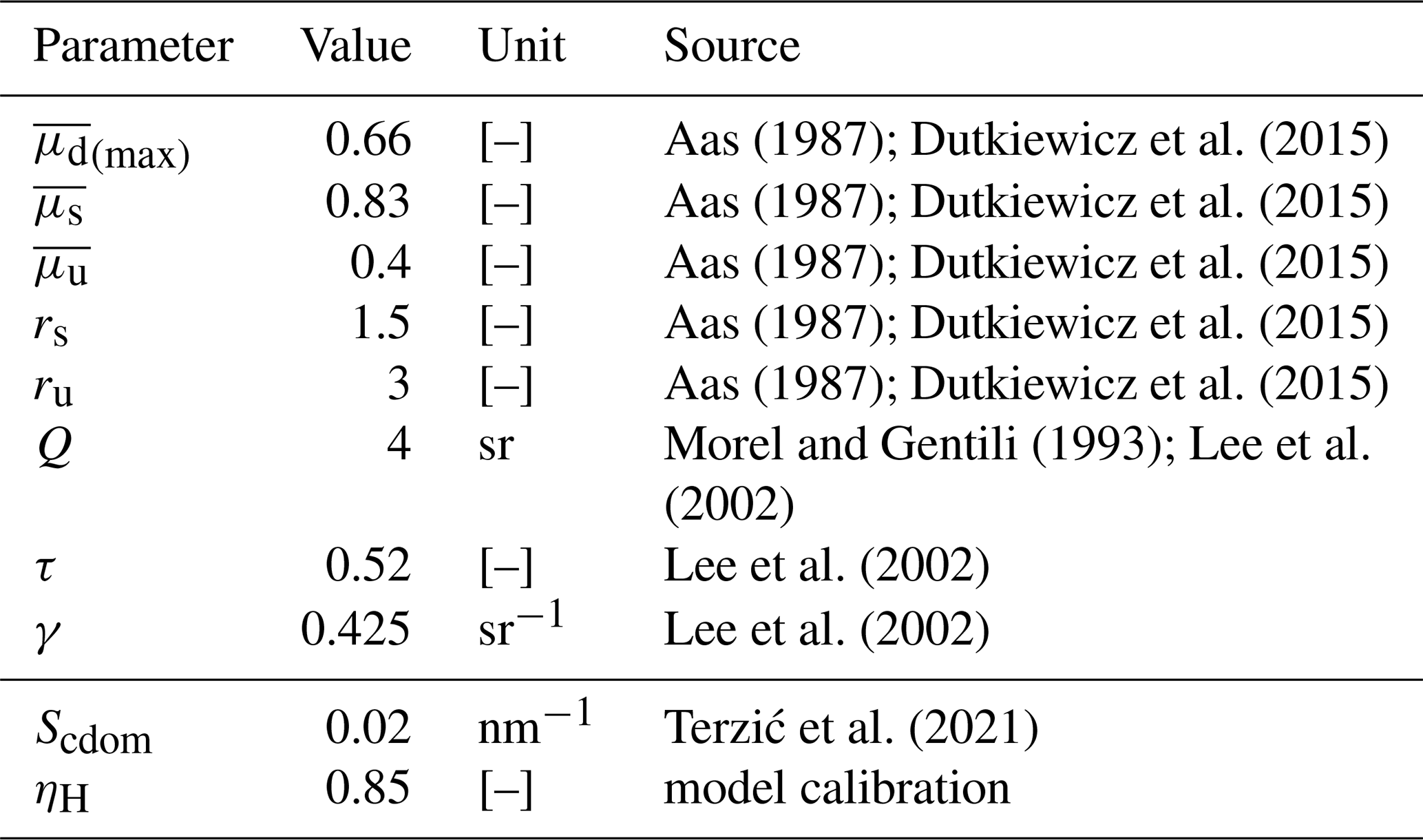
With τ the radiance transmittance of the interface and γ the internal reflection coefficient (Bai et al., 2020). R_RS is the quantity that is then comparable to remote-sensing data. Representative values of the coefficients Q, τ and γ can be found in Table 1.

Aas (1987); Dutkiewicz et al. (2015)Aas (1987); Dutkiewicz et al. (2015)Aas (1987); Dutkiewicz et al. (2015)Aas (1987); Dutkiewicz et al. (2015)Aas (1987); Dutkiewicz et al. (2015)Morel and Gentili (1993); Lee et al. (2002)Lee et al. (2002)Lee et al. (2002)Terzić et al. (2021)

Table 1 Model parameters for the Black Sea implementation of the RT model.

The RT model described in this section can be used as an observation operator for the physical-biogeochemical framework, as it serves as a link between the modelling framework and the observations. We talk then of a one-way configuration, when information from the RT module is not used by the other components of the modelling framework. The RT module is two-way coupled if the simulated irradiances are used in the simulation of temperature and primary production in the coupled model. In this article, we consider the two-way configuration of the coupled model. For reference, the one-way coupling was used in Macé et al. (2025).

2.2 Integration within the NEMO framework

The total scalar irradiance budget E_tot is computed by the RT module over its entire spectral range and is used as the source term of Eq. (10) which describes the evolution of temperature T through the computation of the heat budget. In the classic NEMO radiative schemes, E_tot is derived only from the downward stream of irradiance computed over two to four wavebands. In this formulation, the three streams of irradiance appear in the equation and the amount of wavebands is increased due to the finer spectral resolution, as in Eq. (11).

$$\begin{array}{}\text{(10)}& {\displaystyle \frac{\partial T}{\partial t}}={\displaystyle \frac{{\mathit{\eta }}_{\mathrm{H}}}{c_p{\mathit{\rho }}_{\mathrm{0}}}}{\displaystyle \frac{\partial E_{\text{tot}}}{\partial z}}\text{(11)}& {\displaystyle }{E}_{\text{tot}}=\sum _{\mathit{\lambda }}\left({\displaystyle \frac{E_{\mathrm{d}}\left(\mathit{\lambda }\right)}{\stackrel{\mathrm{‾}}{{\mathit{\mu }}_{\mathrm{d}}}}}+{\displaystyle \frac{E_{\mathrm{s}}\left(\mathit{\lambda }\right)}{\stackrel{\mathrm{‾}}{{\mathit{\mu }}_{\mathrm{s}}}}}-{\displaystyle \frac{E_{\mathrm{u}}\left(\mathit{\lambda }\right)}{\stackrel{\mathrm{‾}}{{\mathit{\mu }}_{\mathrm{u}}}}}\right)\end{array}$$

with c_p the heat capacity of water, ρ₀ the density of water and η_H a constant dimensionless tuning factor. ΔE_d(λ), ΔE_s(λ) and ΔE_u(λ) respectively represent the difference in irradiance between the top and bottom of the model grid cell. The parameter η_H is a tuning parameter meant to account for the fraction of absorbed irradiance that is actually used to heat water. In reality, some of the energy that is lost as light propagates in seawater is used by phytoplankton for photosynthesis or to degrade particles and minerals (Del Vecchio and Blough, 2002). In general, the parameter η_H should be very close to 1, as virtually all radiation participates in the heating of sea water (Mobley et al., 2015). Here, it is also added as a way to tune the temperature feedback and compensate temperature biases that could arise. It should be calibrated accordingly with observations for each use case. The technical description of the temperature feedback within the code is presented in Appendix B. This temperature feedback is proposed as an additional scheme for RT that can be used in place of the default schemes defined in the traqsr.F90 source file (e.g. two- or three-band models). This scheme is activated by setting the flag ln_qsr_RT = .true. in the namtra_qsr namelist. The parameter η_H must be set in the nam_RADTRANS namelist.

2.3 Inherent Optical Properties

Solving Eqs. (1)–(3) requires information on the profiles of seawater IOPs: coefficients of spectral absorption a, forward scattering b_f, and backscattering b_b. These variables are estimated by a biogeochemical model coupled with NEMO or could be forced into the model. In the three-stream RT model, we account for four optically active constituents that contribute to absorption and scattering: pure water, phytoplankton, detritic non-algal particles, and coloured dissolved organic matter (CDOM). We assume that the latter only contributes to absorption (Dutkiewicz et al., 2015; Álvarez et al., 2023). IOPs are derived from the sum of optical properties of seawater constituents that contribute to absorption and scattering.

$$\begin{array}{}\text{(12)}& {\displaystyle }\begin{array}{rl}a(\mathit{\lambda },z)& =a_{\mathrm{w}}(\mathit{\lambda },z)+a_{\text{phy}}(\mathit{\lambda },z)+a_{\text{prt}}(\mathit{\lambda },z)\\ & +a_{\text{cdom}}(\mathit{\lambda },z)\end{array}\text{(13)}& {\displaystyle }{b}_{\mathrm{f}}(\mathit{\lambda },z)=b_{\text{f,w}}(\mathit{\lambda },z)+b_{\text{f,phy}}(\mathit{\lambda },z)+b_{\text{f,prt}}(\mathit{\lambda },z)\text{(14)}& {\displaystyle }{b}_{\mathrm{b}}(\mathit{\lambda },z)=b_{\text{b,w}}(\mathit{\lambda },z)+b_{\text{b,phy}}(\mathit{\lambda },z)+b_{\text{b,prt}}(\mathit{\lambda },z)\end{array}$$

Many studies have focused on the optical properties of pure seawater (a_w, b_f,w, and b_b,w), and these are now well documented (Pope and Fry, 1997; Morel et al., 2007; Mason et al., 2016). Outside of the visible range, high absorption by seawater does not allow radiation to propagate further than a few metres. In the visible range, absorption is lower and the contribution of other constituents becomes relevant. We use the absorption and scattering spectra from lab experiments described in Pope and Fry (1997), and we consider symmetric seawater scattering as in Gregg and Rousseaux (2016), with equal scattering and backscattering. Absorption and scattering spectra are considered accurate, and are provided in Fig. 1.

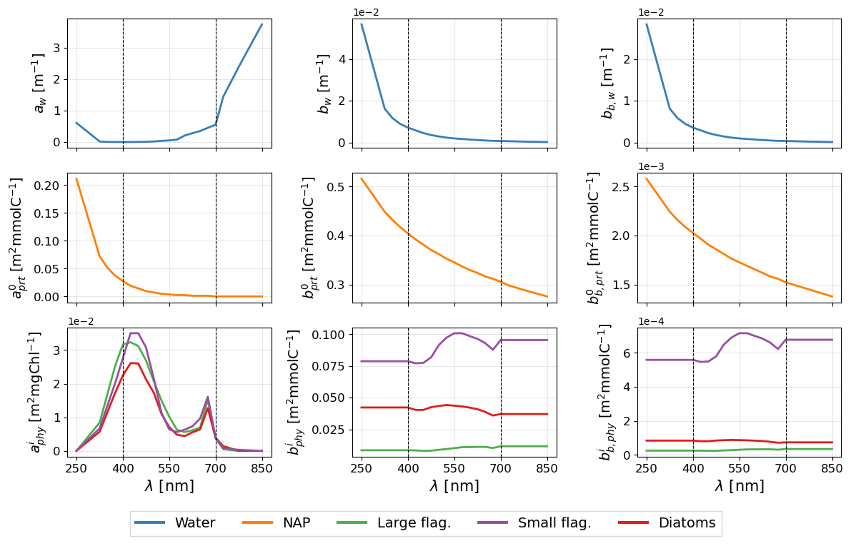
Figure 1 Spectra for the optical properties for water (top) (Pope and Fry, 1997), non-algal particles (centre) (Gallegos et al., 2011; Álvarez et al., 2022) and the three PFTs defined in BAMHBI: diatoms, small flagellates and large flagellates (bottom) (adapted from Dutkiewicz et al., 2015; Álvarez et al., 2022).

The absorption and scattering by phytoplankton (a_phy, b_f,phy, and b_b,phy) are the sum of the contributions of the phytoplankton species considered in the model, as in Eqs. (15)–(17). In biogeochemical models, phytoplankton species are typically grouped in phytoplankton functional types (PFTs) based on common traits and affinities for light or nutrients. For each PFT, absorption and scattering are computed from phytoplankton concentration and reference spectra. The number of PFTs considered in the model can be adjusted depending on the application of the model. Examples of spectra for PFTs that are considered in the use case of this article are presented in Fig. 1.

$$\begin{array}{}\text{(15)}& {\displaystyle }{a}_{\text{phy}}(\mathit{\lambda },z)=\sum _i{a}_{\text{phy}}^i\left(\mathit{\lambda }\right){\text{CHL}}^i\left(z\right)\text{(16)}& {\displaystyle }{b}_{\text{f,phy}}(\mathit{\lambda },z)=\sum _i{b}_{\text{f,phy}}^i\left(\mathit{\lambda }\right)C_{\text{chl}}^i\left(z\right)\text{(17)}& {\displaystyle }{b}_{\text{b,phy}}(\mathit{\lambda },z)=\sum _i{b}_{\text{b,phy}}^i\left(\mathit{\lambda }\right)C_{\text{chl}}^i\left(z\right)\end{array}$$

Where $a_{\text{phy}}^i$ is the reference absorption in units of m² mg Chl⁻¹, $b_{\text{f,phy}}^i$ and $b_{\text{b,phy}}^i$ are the reference scattering in units of m² mmol C⁻¹, CHLⁱ is the chlorophyll concentration for each PFT in units of mg Chl m⁻³ and $C_{\text{chl}}^i$ is the carbon content in each PFT in units of mmol C m⁻³. Phytoplankton absorption and scattering spectra are taken from the results of the literature review presented in Álvarez et al. (2022), that includes field observations in the Mediterranean Sea. We may therefore expect uncertainties arising from the difference in the definition of PFTs across basins and models.

The optical properties of non-algal particles (a_prt, b_f,prt, and b_b,prt) are derived from the concentration of detritus, or non-living particulate organic carbon (POC) as in Eqs. (18)–(20). It acts as a proxy for particle concentration, under the assumption that the particles are uniform in size and shape (Dutkiewicz et al., 2015). The reference coefficients ($a_{\text{prt}}^{\mathrm{0}}$, $b_{\text{f,prt}}^{\mathrm{0}}$, and $b_{\text{b,prt}}^{\mathrm{0}}$) are derived from Gallegos et al. (2011) and Álvarez et al. (2022) and their spectra are provided in Fig. 1. This model aggregates data from various field campaigns to provide a model of absorption and scattering by non-algal particles.

$$\begin{array}{}\text{(18)}& {\displaystyle }{a}_{\text{prt}}(\mathit{\lambda },z)=a_{\text{prt}}^{\mathrm{0}}\left(\mathit{\lambda }\right)\text{POC}\left(z\right)\text{(19)}& {\displaystyle }{b}_{\text{f,prt}}(\mathit{\lambda },z)=b_{\text{f,prt}}^{\mathrm{0}}\left(\mathit{\lambda }\right)\text{POC}\left(z\right)\text{(20)}& {\displaystyle }{b}_{\text{b,prt}}(\mathit{\lambda },z)=b_{\text{b,prt}}^{\mathrm{0}}\left(\mathit{\lambda }\right)\text{POC}\left(z\right)\end{array}$$

Absorption by CDOM (a_cdom) is calculated from a reference profile at a prescribed wavelength. We choose the 412 nm wavelength as the reference here as data for irradiance streams are often available in this waveband. The reference profile can either be forced into the model of derived from an estimation of CDOM concentration provided by a biogeochemical model. CDOM absorption is then propagated in other wavebands with the following exponential law.

$$\begin{array}{}\text{(21)}& a_{\text{cdom}}\left(\mathit{\lambda }\right)=a_{\text{cdom}}\left({\mathit{\lambda }}_{\text{ref}}\right)e^{-S_{\text{cdom}}(\mathit{\lambda }-{\mathit{\lambda }}_{\text{ref}})}\end{array}$$

With a_cdom the reference forcing profile at λ_ref=412 nm and S_cdom the slope factor describing the exponential decrease in absorption in longer wavebands (Twardowski et al., 2004; Kitidis et al., 2006; Dutkiewicz et al., 2015). Thus CDOM principally absorbs in short wavelengths. A literature review on S_cdom values can be found in Terzić et al. (2021). The values for S_cdom and all the other parameters of the RT model need to be specified by the user depending on the application case of the model.

2.4 Stochastic version of the radiative transfer model

In addition to the deterministic version of the RT module, we provide a stochastic version of the RT model, that offers the possibility to consider uncertainties in the modelling of IOPs. The stochastic version of the model relies on the introduction of stochastic perturbations in the parameterisation of the IOPs, based on the generic approach developed by Brankart et al. (2015) that describes its use within the NEMO model. This approach has later been used in Garnier et al. (2016) and Popov et al. (2024), showing its ability to generate variable dispersions that are consistent with uncertainties in biogeochemical variables through the perturbation of biogeochemical parameters. It was presented in Macé et al. (2025) where the RT module was used in a one-way coupled configuration (i.e., as an observation operator). Perturbations in the IOPs are meant to account both for uncertainties in the specific coefficients for absorption and scattering (as in Eqs. 15–21) and on uncertainties in chlorophyll, non-algal particles, and CDOM concentrations fed to the RT model. First-order autoregressive processes are used to generate 2D stochastic perturbation fields that are multiplied by the 2D fields of IOPs. The same perturbation is applied to all vertical levels. The method for perturbing the IOPs is detailed in Macé et al. (2025). We use log-normal distributions for the perturbations to be consistent with the tendency of optical variables to follow log-normal distributions (Vervatis et al., 2021). Transformations to derive the mean μ₀ and standard deviation σ₀ of the initial Gaussian distribution are given following Eqs. (22) and (23) with σ the standard deviation of the final log-normal distribution centred on 1.

$$\begin{array}{}\text{(22)}& {\displaystyle }{\mathit{\mu }}_{\mathrm{0}}=-{\displaystyle \frac{{\mathit{\sigma }}^{\mathrm{2}}}{\mathrm{2}}}\text{(23)}& {\displaystyle }{\mathit{\sigma }}_{\mathrm{0}}^{\mathrm{2}}=\ln (\mathrm{1}+{\mathit{\sigma }}^{\mathrm{2}})\end{array}$$

3 Framework for application in the Black Sea

The RT module presented in Sect. 2, including its stochastic version, has been tested in the Black Sea where NEMO-BAMHBI is run in forecasting and reanalysis mode in the frame of the Copernicus Marine Service. Its inclusion as an additional module to the BAMHBI model, which upgrades the current version of BAMHBI, is presented in this section. The RT model has been calibrated thanks to Biogeochemical (BGC)-Argo floats that have been deployed in the Black Sea for more than a decade. The IOPs necessary to compute the spectral irradiance are provided based on NEMO-BAMHBI variables. We introduce the coupling of the RT module with the BAMHBI framework, through the computation of IOPs and the surface radiative forcing.

In the following, we present a comparison of model runs using two schemes for the modelling of light.

• The three-stream radiative transfer model, introduced in Sect. 2 with Eqs. (1)–(21), hereafter called RT model.

• The attenuation scheme embedded in the BAMHBI model, that simulated light attenuation in three wavebands. It is briefly presented for reference in Sect. 3.1 with Eqs. (24) and (25), and hereafter called “simple optics”.

3.1 The BAMHBI model

The BiogeochemicAl Model for Hypoxic and Benthic Influenced areas (BAMHBI) is a marine biogeochemical model that describes the cycles of carbon, nitrogen, phosphorus, silicon and oxygen through the modelling of the marine foodweb from bacteria up to mesozooplankton (Grégoire et al., 2008; Grégoire and Soetart, 2010). A complete technical description of the BAMHBI model can be found in Grégoire et al. (2026). It solves three PFTs, two zooplankton types, and the microbial loop with several classes of detritic materials. The BAMHBI model is appropriate to model low-oxygen environments, explicitly representing the anoxic layer in the case of the Black Sea.

The current version of BAMHBI uses a simpler optics model that only simulates direct downward streams of light in three large wavebands, as described in Capet (2014). The visible spectral range is split into two bands, differentiating radiation between a short and a long waveband. The third band is in the infrared range. The absorption and scattering of light by the three phytoplankton groups and organic particles is considered as described in Grégoire et al. (2026) and the absorption of CDOM is parameterised as a function of salinity to represent the higher CDOM absorption found at river mouths. Surface radiation is forced from the regional configuration of an atmospheric model. At sea surface, the reflected fraction of irradiance, due to surface albedo, is removed to obtain radiation just below sea surface. Below the surface, a single irradiance stream E_fo is attenuated following Beer's law with an absorption coefficient a_fo derived from chlorophyll concentration, particulate organic carbon (POC), and salinity, in each of the three wavebands. The reference “simple optics” configuration is therefore defined with Eqs. (24) and (25), with a_fo.w, a_fo.chl, a_fo.poc and a_fo.cdom the respective absorption coefficients by seawater, chlorophyll, detritus, and CDOM.

$$\begin{array}{}\text{(24)}& {\displaystyle }{a}_{\text{fo}}=a_{\text{fo.w}}+a_{\text{fo.chl}}+a_{\text{fo.poc}}+a_{\text{fo.cdom}}\text{(25)}& {\displaystyle \frac{\mathrm{d}{E}_{\text{fo}}\left(z\right)}{\mathrm{d}z}}=-a_{\text{fo}}{E}_{\text{fo}}\left(z\right)\end{array}$$

We aim to build on top of the current version of BAMHBI described in Grégoire et al. (2026) by extending it with the three-stream RT scheme described in Sect. 2 as an additional optional module. The code for the version of BAMHBI extended with RT modelling is described in Appendix B. When BAMHBI is used with the RT module, it provides the IOPs to solve the direct and diffuse spectral radiation according to Eqs. (1)–(6). Three PFTs are considered: dinoflagellates, smaller flagellates, and diatoms. These species are dominant in the Black Sea (Silkin et al., 2021). Data for the reference spectra are adapted from Álvarez et al. (2022) to match the PFTs simulated in BAMHBI. Specific absorption and scattering spectra for phytoplankton are provided in Fig. 1. a_phy, b_phy, and b_b,phy are therefore calculated as the sum of contributions from these three PFTs following Eqs. (15)–(17). The optical properties of non-algal particles are computed using POC that is explicitly simulated in BAMHBI, following Eqs. (18)–(20).

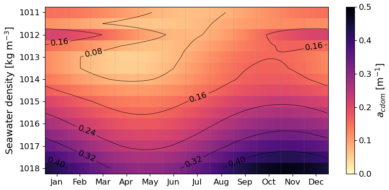
CDOM is not explicitly simulated in BAMHBI, which does not allow to compute its contribution to absorption. Here we decide to directly force CDOM absorption into the model. This forcing is built using BGC-Argo data in the Black Sea between 2017 and 2020. Among the collected data, we use profiles of chlorophyll concentration and particulate backscattering coefficient at 700 nm to derive the optical properties of phytoplankton and non-algal particles. We use CDOM fluorescence (fDOM) profiles to impose the shape of CDOM absorption profiles, assuming that the absorption capability of CDOM is uniform in the vertical dimension. The relationship imposed in this forcing is therefore $a_{\text{cdom}}=A\times \text{fDOM}$, with the coefficient A constant on the vertical and to be determined independently for each profile. Since BGC-Argo floats provide measurements of downward irradiance in three wavebands (centred on 380, 412 and 490 nm), we use the 1D test model to optimise CDOM absorption to best match the data. Given the large amount of available BGC-Argo profiles, we maintain seasonality in the resulting CDOM absorption forcing. Rather than having a forcing depending on depth, we create a lookup table that defines a_cdom based on density (ρ) and seasonality, to exhibit seasonal and spatial variations in the composition of seawater. A Hovmöller representation of this table is shown in Fig. 2 with a further description of the method used to derive this contribution in Appendix A. Table 1 provides the values of the parameters used in this NEMO-BAMHBI configuration.

Figure 2 CDOM absorption forcing with regard to seawater density and day of the year.

When coupled, the RT model provides BAMHBI the scalar irradiance that is available to phytoplankton for photosynthesis. It is defined as the integrated scalar irradiance in the visible range (i.e. between 400 and 700 nm) as in Eq. (26). E₀ (in W m⁻²) is the fraction of irradiance available to phytoplankton and is therefore defined from the three streams of irradiance. In situ observations of PAR (photosynthetically active radiation, in $\mathrm{\mu }\mathrm{mol}{\mathrm{s}}^{-\mathrm{1}}{\mathrm{m}}^{-\mathrm{2}}$) are also often available and can be related to E₀ when approximating conversion rates, making it a useful variable for model validation. Following Thimijan and Heins (1983), we use the approximation for daylight conditions described in Eq. (27).

$$\begin{array}{}\text{(26)}& {\displaystyle }{E}_{\mathrm{0}}\left(z\right)=\underset{\mathrm{400}\mathrm{nm}}{\overset{\mathrm{700}\mathrm{nm}}{\int }}\left[{\displaystyle \frac{E_{\mathrm{d}}(\mathit{\lambda },z)}{\stackrel{\mathrm{‾}}{{\mathit{\mu }}_{\mathrm{d}}}}}+{\displaystyle \frac{E_{\mathrm{s}}(\mathit{\lambda },z)}{\stackrel{\mathrm{‾}}{{\mathit{\mu }}_{\mathrm{s}}}}}+{\displaystyle \frac{E_{\mathrm{u}}(\mathit{\lambda },z)}{\stackrel{\mathrm{‾}}{{\mathit{\mu }}_{\mathrm{u}}}}}\right]\mathrm{d}\mathit{\lambda }\text{(27)}& {\displaystyle }\text{PAR}=\mathrm{4.6}\times E_{\mathrm{0}}\end{array}$$

3.2 MAR surface forcing

The RT model needs information on the spectral irradiance at sea surface as a boundary condition. Before reaching the sea surface, the solar irradiance propagates through the atmosphere, where it is already divided into direct and scattered streams. This information is then propagated in the water column according to the IOPs. To provide these boundary conditions, we use spectral shortwave fluxes simulated over the Black Sea area with a regional atmospheric model (Gallée et al., 2013; Grailet et al., 2025). MAR (Modèle Atmosphérique Régional) is a regional climate model used for both weather forecasting and climate studies. For this study, the atmosphere over the Black Sea has been simulated by the MAR version 3.14, which runs with the ECMWF radiative transfer scheme ecRad v1.5.0 (Hogan and Bozzo, 2018). Operational since 2017, ecRad is a flexible radiation scheme which allows users to easily tune its sub-components, such as cloud and gas optics. In particular, ecRad v1.5.0 is capable of running with high-resolution gas optics schemes pre-computed with the ecCKD tool (Hogan and Matricardi, 2022), and the CAMS aerosol specification (Bozzo et al., 2017). As a result, the atmospheric model is able to simulate aerosol optical depth. Aerosol mixing ratios for ecRad are prepared from climatological data. Since late 2022, it has also been capable of producing spectral shortwave fluxes in user-defined bands. Grailet et al. (2025) demonstrated that running MAR v3.14 with ecRad and a high-resolution ecCKD gas optics scheme for the shortwave range can produce realistic spectral shortwave fluxes with respect to ground observations. The spectral bands can be as small as 5 nm wide, as long as they are not finer in resolution than the inner spectral bands of the ecCKD model. The ecRad scheme is also able to separate direct and diffuse irradiances that are later fed to the ocean model.

To simulate the Black Sea, MAR has been configured with a 15 km grid resolution and 24 pressure levels in sigma coordinates that extend from the surface to the lower stratosphere. It has been forced at its lateral boundaries by ERA5 reanalyses (Hersbach et al., 2020) and has been tuned to use a high resolution ecCKD gas-optics scheme in the shortwave range, to produce fine spectral shortwave fluxes. The output spectral bands have been configured to be equivalent to the 33 wavebands used in the ocean RT model, ranging between 250 and 4000 nm. For consistency, we also choose to force ocean physics of the model with outputs from the same MAR simulation: sea level pressure, humidity, 2 m temperature, wind speed and precipitation. The MAR radiative fluxes have been compared against ERA5 reanalyses and PAR ground observations at the Kichinev AERONET station (Moldova). Against ground observations, MAR achieves high correlation (>0.9) and low bias. This validation is not presented in detail here as it is not the focus on the paper. A thorough evaluation of MAR spectral fluxes over a European location is provided in Grailet et al. (2025).

It should be noted that any potential bias in the forcing would not significantly influence the fields of sea surface reflectance that are produced. In fact, reflectance is computed as the ratio of upwelling irradiance to downwelling irradiance (see Eq. 7). This equation can also be understood as the normalisation of upwelling irradiance, influenced by absorption and backscattering, by the forced downwelling irradiance. Despite a difference in incident downwelling irradiance, the fraction of irradiance that is backscattered remains the same, and therefore the ratio between upwelling and downwelling irradiance at sea surface would remain rather similar.

Radiative forcing consists of downward direct E_d.forc and scattered E_s.forc irradiance streams on the sea surface for each wavelength and grid location of the domain. We derive the boundary conditions described in Eqs. (4) and (5) by accounting for sea surface albedo A, taken from the mean monthly albedo dataset for the Atlantic Ocean at 40° N described in Payne (1972).

$$\begin{array}{}\text{(28)}& {\displaystyle }{E}_{\text{d0}}=(\mathrm{1}-A)E_{\text{d.forc}}\text{(29)}& {\displaystyle }{E}_{\text{s0}}=(\mathrm{1}-A)E_{\text{s.forc}}\end{array}$$

3.3 Description of the use case configuration

Based on the initial scheme with simple optics and the three-stream RT scheme, we define three BAMHBI configurations that are described here and analysed in Sect. 4:

• Simple optics: using the one-stream scheme from Capet (2014), detailed in Sect. 3.1. The simple optics scheme is the one that runs with the current version of BAMHBI (Grégoire et al., 2026).

• RT: using the updated “radtrans” model from Dutkiewicz et al. (2015), a three-stream model in thirty-three wavebands, as described in Sect. 2, coupled with NEMO-BAMHBI.

• Stochastic RT: using the stochastic mode of the RT model, presented in Sect. 2.4, and therefore accounting for uncertainties in the modelling of IOPs. The corresponding experiments consist of a 50-member ensemble used to compare time series of sea surface reflectance with in situ data.

With the inclusion of the three-stream RT scheme and the new surface radiative forcing, the deterministic and stochastic RT configurations presented in this article make an extension of the NEMO-BAMHBI modelling framework. The RT module takes inputs from BAMHBI and external forcings, and its outputs are used by both NEMO and BAMHBI. It includes the computation of three new state variables that correspond to the three streams of irradiance, and a diagnostic variable that is the sea surface reflectance.

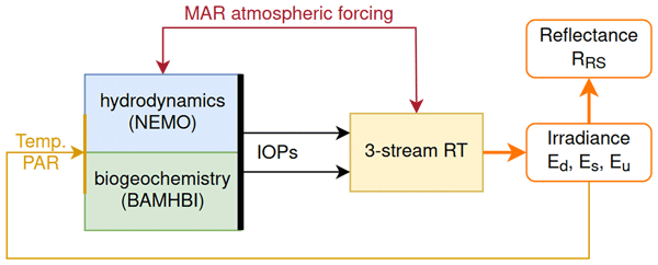
In all experiments, BAMHBI is coupled with NEMO 4.2 on the same horizontal and vertical grids. We use a NEMO configuration for the Black Sea with a horizontal resolution of 15 km and 59 vertical levels distributed unevenly. The layers are thinner close to the surface and thicker in the deeper parts of the basin. Biogeochemical forcings such as river inputs and atmospheric deposition of nutrients (phosphorus, nitrate and ammonium) are based on climatology data. The model is forced with river runoffs that are based on climatology. We assume that there are no exchanges with the Sea of Azov, and the exchanges with the Sea of Marmara at the Bosphorus Strait are set following Stanev and Beckers (1999). In the RT configurations, we consider 33 wavebands ranging between 250 and 4000 nm with a finer 25 nm resolution in the visible range. Temperature and E₀ feedbacks are activated with NEMO and BAMHBI, respectively. In this configuration, the parameter η_H (see Eq. 10) transcribing the fraction of absorbed irradiance that is used to heat the water column is set to 0.85 after calibration of the model with a 1D test model in the Black Sea. Figure 3 provides an overview of the coupled modelling framework for experiments using the RT module.

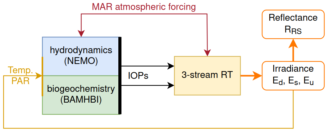
Figure 3 Coupling of the 3-stream RT model within the NEMO-BAMHBI framework. Forcing for physics and surface radiation are provided by a regional MAR simulation (see Sect. 3.2). In a configuration without a biogeochemical model, the IOPs would be forced from external data into the three-stream RT module.

The parameters for the RT module specific to the use case are specified in the nam_RADTRANS namelist. They consist of the parameters defined in Table 1 along with the forced inputs:

• The wavebands and spectral range to be simulated

• The parameters described in Sect. 2: r_s, r_u, μ_d, μ_s, μ_u, Q, τ, γ, η_H

• The absorption and scattering spectra for water, phytoplankton and non-algal particles

• The reference absorption profile for CDOM absorption and the slope coefficient S_cdom

• The surface radiative forcing (downward direct and scattered streams)

4 RT modelling in the Black Sea

This section describes the application of the RT model to the Black Sea using the NEMO-BAMHBI framework. We first investigate the consequences of substituting the RT scheme in the computation of temperature and chlorophyll. This is done through comparison with BGC-Argo and satellite data, and with the former simple optics configurations when available. We then elaborate on the computation of radiometric variables, with an outlook on the uncertainties that arise from the parameterisation of the IOPs. We highlight the benefit of a RT model for linking simulations with observations with the example of a chlorophyll estimate derived from the RT simulated reflectance as estimated in ocean colour inversion algorithms.

4.1 In-water irradiance

In the simple optics configuration, E₀ is simulated from two wavebands in the visible range and with a simple one-stream irradiance model. With the RT configuration, we simulate the irradiance at a higher spectral resolution, providing a more detailed representation of the spectral irradiance. Scatter plots of downwelling irradiance at 380, 412 and 490 nm, simulated by the RT model and observed by BGC-ARGO (between 2017 and 2020) are presented in Fig. 4. In this figure, downwelling irradiances are normalised by their surface values, respectively from observations and model, to focus on radiation absorption independently from potential surface radiation biases. Regressions are computed to evaluate the agreement between sub-surface datasets. We use hourly model outputs in order to consistently match in situ data despite the sub-daily variability of irradiance. In the model, the downwelling irradiance is defined as the sum of the direct and downward scattered streams of irradiance. The data shown are the logarithms of normalised irradiances in order to compare orders of magnitude and give weight to both higher values at the surface and lower values in the depth. We find that the simulation of the irradiance streams is very consistent with the observed data despite an underestimation of irradiance at 380 nm. The agreement in the 412 and 490 nm wavebands is very good with regression slopes close to 1. At 380 and 412 nm, and close to the surface, attenuation seems larger in the model that in BGC-Argo profiles. This corresponds to the spectral range in which CDOM dominates absorption. The bias is larger at 380 nm and decreases with the wavelength while RMSEs are of similar magnitude.

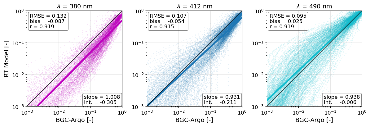
Figure 4 Logarithm of normalised downwelling irradiance from BGC-Argo data and the RT model in the RT configuration at the location of BGC-Argo floats between 2017 and 2020, for the upper 100 m. Irradiance measurements are normalised by the closest available value to the surface. The indexes of the BGC-Argo floats used are 6901866, 6903240 and 7900591. RMSE, correlation coefficient (r), regression slope and intercept are displayed for each wavelength. Scatter plots show 19 556, 25 628 and 43 268 points respectively for the 380, 412 and 490 nm wavebands.

BGC-Argo profiles also provide PAR data, which can be converted to scalar irradiance E₀. It should be noted that the method used to compute E₀ is not the same in both configurations, leading to differences at sea surface even though the forcing is the same. In the simple optics configuration, E₀ is defined as 46 % of the total solar radiation, while in the three-stream model it is defined as the integration of solar radiation between 400 and 700 nm. The surface E₀ tends to be higher in the RT configuration. To analyse the attenuation of E₀ profiles, we focus here on normalised profiles with regard to the surface values. Figure 5 presents a scatter plot with data from normalised E₀ profiles simulated by the simple optics and the RT configurations with BGC-Argo data between 2017 and 2020. The agreement with BGC-Argo data for normalised E₀ is very good, with a regression slope in the scatter plot of over 0.9. Since this slope is lower than 1, the difference between model outputs and BGC-Argo data is explained by a higher absorption in the model close to the surface and too low in depth. The use of a RT model has a rather neutral effect on the simulation of E₀ profiles, with lower biases and similar errors. The performance of both models remains close and the change in scheme maintains the simulation of E₀.

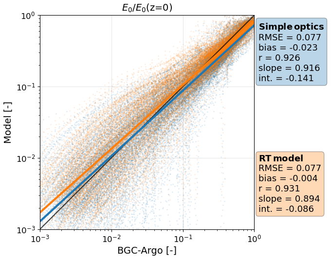
Figure 5 Logarithm of normalised E₀ derived from BGC-Argo PAR data with the simple optics and RT configurations at the location of BGC-Argo floats between 2017 and 2020, for the upper 100 m. RMSE, bias, correlation coefficient (r), regression slope and intercept are displayed. Scatter plots show 36 376 points. Normalisation is performed relative to the maximum value of the E₀ profile, which is the closest data from sea surface.

4.2 Simulation of temperature profiles

In this section, we assess the influence of solving radiative transfer with a three-stream RT scheme on temperature. In the coupling with NEMO, the irradiance streams are used to compute the evolution of temperature in the model following Eq. (10). This implies that a change in the irradiance streams influences physics, which in turn influences the biogeochemistry and IOPs. Calibration of the η_H parameter, which intervenes in Eq. (10), is performed in such a way that the temperature profiles in the RT configuration remains consistent with BGC-Argo profiles for our Black Sea configuration. As such, we do not expect large differences between the simple optics and RT configurations. While η_H should normally be close to one, model validation against in situ data suggested to lower this value to match temperature profiles.

To evaluate the influence of this feedback on temperature from the RT to the physics, we consider the sea surface temperature (SST) from both model configurations and from BGC-Argo data, where it is defined as the average temperature in the top 5 m. This allows the inclusion of BGC-Argo data profiles that do not have samples right under the surface. The left panel of Fig. 6 shows a scatter plot of the data from 418 profiles between 2017 and 2020. It evidences the good agreement between modelled SST and in situ data, with correlations higher than 0.99 with both configurations. Statistics for bias and RMSE are presented in Table 2.

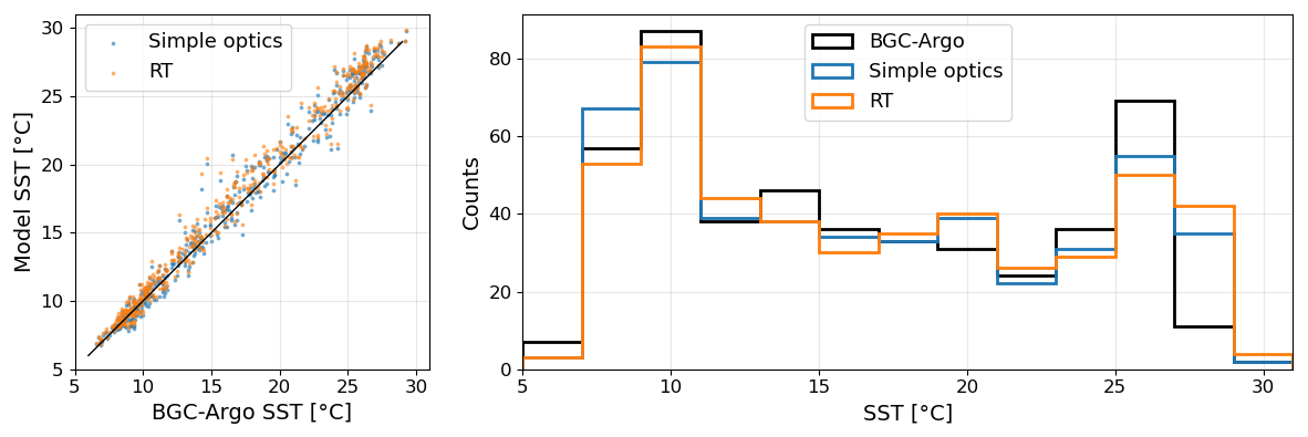
Figure 6 Scatter plot and distributions of SST from BGC-Argo floats between 2017 and 2020 and compared to the simple optics and RT configurations, respectively in blue and orange. Bins are taken following the vertical grid of the model. 478 profiles are considered.

Table 2 Bias, RMSE and correlation of SST, normalised E₀ and surface chlorophyll from simulated variables against BGC-ARGO data. Profiles are taken from floats 6901866, 6903240 and 7900591 between 2017 and 2020.

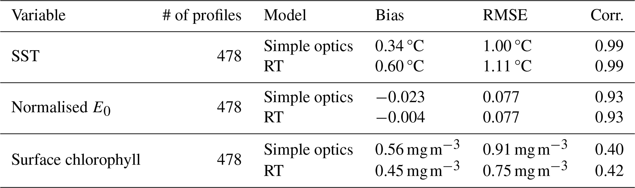
The right-hand side panel of Fig. 6 shows the distributions of SST in the three datasets that are compared, showing that distributions of SST remain rather similar. Here, the bias and RMSE in SST slightly increase between the simple optics and the RT configuration. The differences remain rather small compared to sea temperatures and are considered acceptable to validate the feedback loop from the RT model to the physics. Several other diagnostics have been checked, although not shown in this paper as it is not the core of the work. The simulation of the cold intermediate layer cold content (CCC) and the mixed layer depth remain consistent over the four years of simulation, as well as thermocline and halocline depths.

4.3 Simulation of chlorophyll

As for temperature, the IOPs of the upper ocean layers dictate the amount of light received by the lower layers, and therefore the ability for phytoplankton to develop ialong the water column. Figure 7 compares the distributions of surface chlorophyll simulated in the RT configuration and from BGC-Argo data. For comparison, results from the simple optics configuration are given. The BGC-Argo chlorophyll dataset is corrected following Ricour et al. (2021), to reduce bias in chlorophyll profiles. The statistics for this comparison are presented in Table 2.

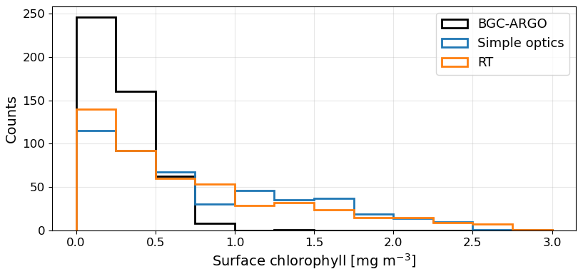
Figure 7 Distributions of surface chlorophyll from BGC-Argo floats (in black) between 2017 and 2020. Distributions of matching surface chlorophyll from the simple optics and RT configurations are respectively shown in blue and orange. 478 profiles are represented here for the simple optics and RT configurations. Bin width is here set to 0.25 mg m⁻³.

The use of the RT module slightly improves the simulation of surface chlorophyll, although some bias remains. The series of surface chlorophyll is better correlated with the measured data, and the RMSE decreases by 0.16 mg m⁻³. As shown in Fig. 7, the model still tends to overestimate surface chlorophyll concentration on average with a positive bias that remains. One of the reasons for this bias is the overestimation of blooms in the biogeochemical model in winter and spring, which is not fully corrected by using the RT module.

4.4 Sea surface reflectance

The most important addition that comes with the RT configuration is the simulation of sea surface reflectance fields. We use remote-sensing data at the basin scale to assess the ability of the model to produce distributions of sea surface reflectance that are consistent with observations. Figures 8–10 respectively present the monthly distributions of R_RS at λ=490, 555 and 670 nm in simulated and remote-sensing data, in 2018. Data are taken from the daily satellite product throughout the basin. In the beginning of the year, we notice that the distribution of reflectances at 490 nm is more spread out in the satellite data than in the simulation. The model is able, on average, to simulate the correct R_RS(490), but is not always able to reach higher and lower values for reflectance. Noticeably in February, some high values of reflectance are missing. We believe they correspond to localised high reflectances on the northeastern coast of the basin that appear in the satellite data and are underestimated in the model (not shown in the figures). From May to July, the model largely underestimates R_RS(490). This corresponds to the period during which coccolithophores bloom in the Black Sea (Kubryakov et al., 2021). This signal is not picked up by the model, which explains the bias for those three months. From August and until the end of the year, distributions from the model are mostly in agreement with the data despite a noticeable overestimation of sea surface reflectance, hinting at the fact that the model is more reliable when simulating reflectance outside of blooming conditions.

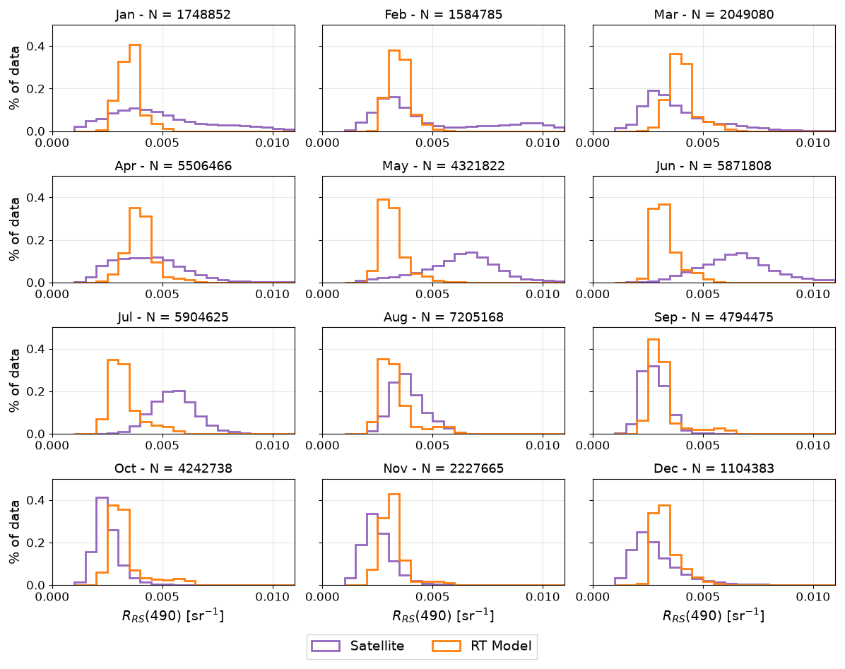
Figure 8 Monthly distributions of sea surface reflectance at 490 nm in 2018 across the Black Sea basin, from the RT configuration (in orange) and remote-sensing (in blue). Simulated reflectance is interpolated at the location of available remote-sensing data.

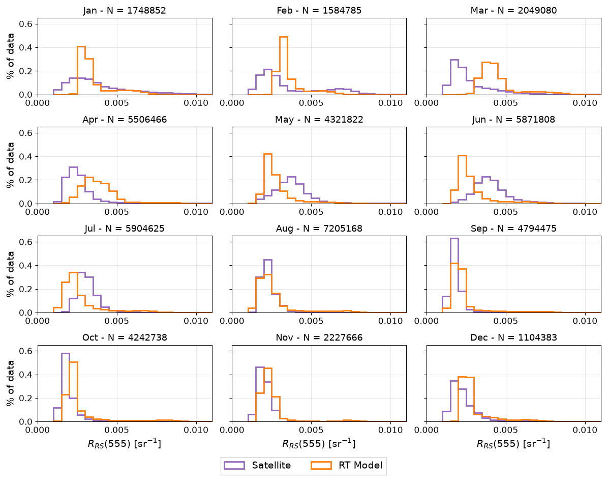
Figure 9 Monthly distributions of sea surface reflectance at 555 nm in 2018 across the Black Sea basin, from the RT configuration (in orange) and remote-sensing (in blue). Simulated reflectance is interpolated at the location of available remote-sensing data.

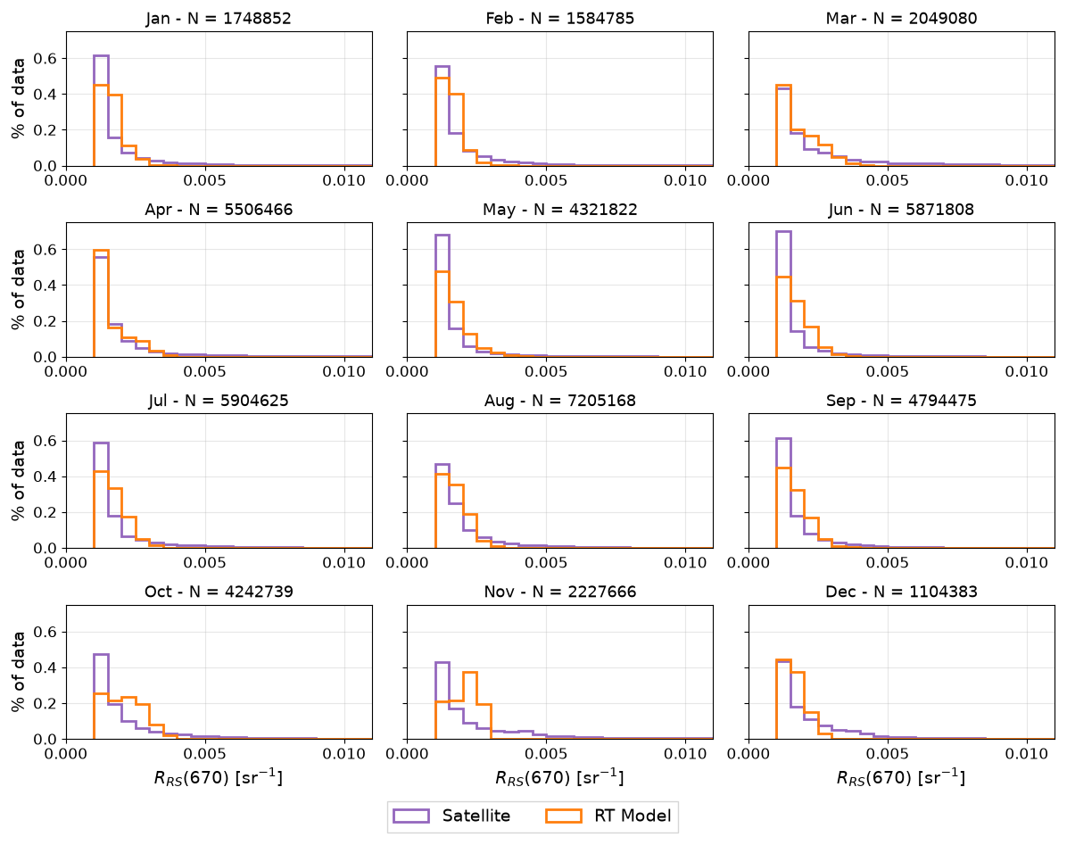
Figure 10 Monthly distributions of sea surface reflectance at 670 nm in 2018 across the Black Sea basin, from the RT configuration (in orange) and remote-sensing (in blue). Simulated reflectance is interpolated at the location of available remote-sensing data.

At 555 nm (Fig. 9), we also notice a thinner spread in the simulated reflectances compared to the satellite data at the beginning of the year. The March and April panels seem to indicate that a bloom is observed later in the model than in the observations. The influence of the coccolithophore bloom that is not picked up by the model is less intense at 555 nm, and becomes nearly insignificant at 670 nm. Then, we find distributions of reflectances that are consistent with observations from August and until the end of the year. At 670 nm, we notice lower reflectances in particular because of higher absorption by water. The distributions are consistent for most of the year until some differences appear in the autumn. At this wavelength, the influence of phytoplankton and CDOM is much lower. Non-algal particles are the main driver of optical properties. The overestimation of reflectances in autumn could indicate concentrations of non-algal particles that are higher in the model than observed, thus leading to increased backscattering and reflectance signal.

In general, the model is able to simulate the main trends in sea surface reflectance at the basin scale. The agreement is best at longer wavelengths such as 670 nm, where the influence of CDOM and phytoplankton is lower. At 490 and 555 nm, some features are misrepresented. The main differences come from the intensity of the blooms and their timing. The model presents less variability compared to the satellite product, keeping the simulated reflectances close to their mean seasonal values. The 490 nm wavelength falls within the spectral range of high backscattering by phytoplankton, allowing us to assess the influence of blooms on the simulated reflectance with this band. The 555 nm wavelength also provides valuable information on blooms in the basin, with also a lower influence of CDOM than at 490 nm. In the 670 nm waveband, the agreement between simulated reflectances and observations appears to be better throughout the year.

We compare for the whole basin in Fig. 11 that shows maps of R_RS at 490 and 555 nm for the 27 October 2018 on the left and central panels. This date is chosen because of the absence of clouds that limits the spatial coverage of the satellite product, and to illustrate a situation where we observe bias in the reflectances, but not significantly in the reflectance-derived chlorophyll. This brings the idea that working with sea surface reflectance ratios could provide a better agreement between model and observations. As expected, we notice higher reflectances in the northwestern shelf where the biological activity is higher for most of the year. In late October, outside of blooming conditions in the deep basin, we notice a rather low bias when comparing with remote-sensing data. This bias is here positive, which is in agreement with the pattern evidenced in Figs. 8 and 9. The bias is greater on the shelf where the increase in reflectance in the model (compared to the deeper areas of the basin) is likely too high compared to observations. It should be noted that the bias on the shelf is rather high, of the same order of magnitude as the absolute values of reflectances.

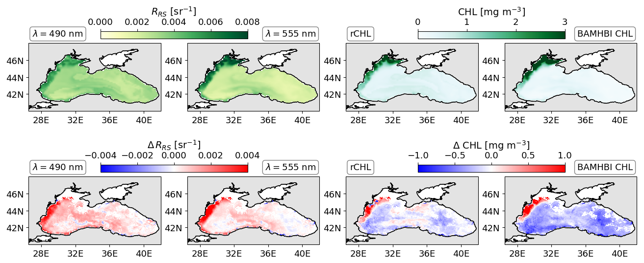
Figure 11 On the top row, maps of simulated R_RS(490) (1st column), R_RS(555) (2nd column), rCHL (3rd column) and BAMHBI chlorophyll (4th column) for the 27 October 2018. On the bottom row, difference with the remote-sensing product.

4.5 Reflectance-derived surface chlorophyll

Algorithms have been developed to derive biological quantities from reflectance fields, in particular to take advantage of remote-sensing data. In the Black Sea, Zibordi et al. (2015) proposed a method to provide surface chlorophyll concentration fields based on reflectance. This method combines a band-ratio algorithm and a neural network approach that is mainly used for more complex coastal waters. This combined method is used by the Copernicus Marine Service to provide surface chlorophyll products for the Black Sea. Using the reflectance simulated by our RT model, we can mimic the band-ratio algorithm in order to compute a new estimate of surface chlorophyll concentration (Kajiyama et al., 2018). This algorithm uses the 490 and 555 nm wavelengths, respectively representative of blue and green. In the following, we refer to this surface chlorophyll estimate as reflectance-derived chlorophyll rCHL:

$$\begin{array}{}\text{(30)}& \log \left(\text{rCHL}\right)=\sum _{k=\mathrm{0}}^{\mathrm{3}}{c}_k\times {\left[\log \left({\displaystyle \frac{R_{\text{RS}}\left(\mathrm{490}\right)}{R_{\text{RS}}\left(\mathrm{555}\right)}}\right)\right]}^k\end{array}$$

The coefficients c_k are provided in Kajiyama et al. (2018) for the Western Black Sea. We extrapolate and use these coefficients for the entire basin here. Reflectance-derived chlorophyll is not independent of the chlorophyll dynamically simulated in BAMHBI because the latter intervenes in the computation of IOPs. However, it provides a quantity that is more closely linked to satellite data by its very definition, using reflectance data. Since Q is parameterised with a constant value, it does not appear in Eq. (30). Although the BDRF coefficient Q should spectrally vary, we assume that it does not differ significantly between close wavebands, so that Q can be removed from the equation.

The right-hand side panels of Fig. 11 show the resulting field of rCHL for the 27 October 2018 and the deviation with the satellite product. In this case, our model tends to underestimate the surface chlorophyll concentration in the deep basin and overestimate it in coastal areas. Although the coastal overestimation is rather consistent seasonally, the underestimation in the deep basin occurs primarily during autumn and winter, whereas a slight overestimation tends to occur in spring and summer, in agreement with the distributions of surface chlorophyll presented in Fig. 12.

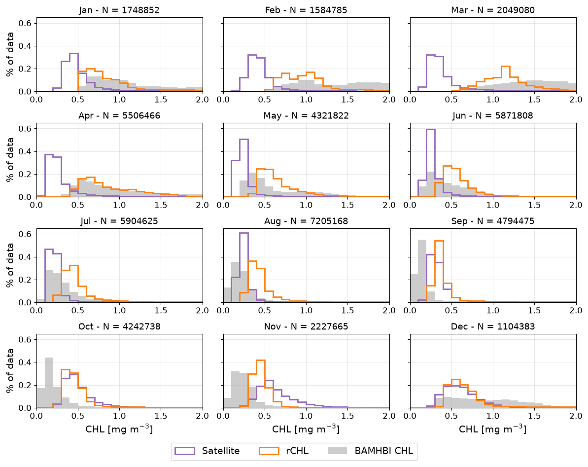
Figure 12 Monthly distributions of reflectance-derived chlorophyll in 2018 across the Black Sea basin from the RT configuration (in orange) against BAMHBI chlorophyll (in grey) and remote-sensing surface chlorophyll (in blue). Simulated rCHL from the RT configuration is interpolated at the location of available remote-sensing data.

When comparing the distributions of rCHL from our simulation and from the satellite product in Fig. 12, we notice patterns that are very similar to those observed with sea surface reflectance at 490 nm. In this figure, we display both rCHL and the chlorophyll computed dynamically in BAMHBI for reference, considering the mean optical depth of the Black Sea of 10 m (Peneva and Stips, 2005). Chlorophyll concentration can first represent blooms in winter, but then overestimates the magnitude. The estimate of surface chlorophyll remains higher than observations during summer until it agrees well with data between September and the end of the year. We notice that the distributions of rCHL are very different from those of the BAMHBI chlorophyll, which is often too high compared to the remote-sensing data. rCHL agrees better with the satellite product than BAMHBI chlorophyll for most of the year. It should also be noted that, surprisingly, the coccolithophore bloom that is identified in the satellite product of sea surface reflectance does not appear in the surface chlorophyll signal. With the band-ratio algorithm, increases in reflectance in both wavebands cancel out, providing low concentrations. In such conditions, we could assume that the satellite product may be biased.

Figure 13 shows the seasonal evolution of the RMSE between the satellite chlorophyll and the model estimated chlorophyll in the simple optics and RT configurations, along with the reflectance-derived chlorophyll rCHL from the RT configuration. The correlations with the satellite product for all three series are very similar, close to 0.45. Although a change in the RT scheme does not significantly influence surface chlorophyll as computed by BAMHBI, such as illustrated in Fig. 7, we notice a large drop in RMSE for rCHL. The improvement is particularly important during the early spring bloom and is also significant during the rest of the year. Finally, the standard deviation in the surface chlorophyll datasets is much higher than with rCHL. This seems to indicate that rCHL does not tend to overestimate or underestimate surface chlorophyll as much as BAMHBI chlorophyll. The overestimation during blooms is lowered and the underestimation outside of blooms is less visible. On average, it produces better estimates and thus leads to a decreased error throughout the year.

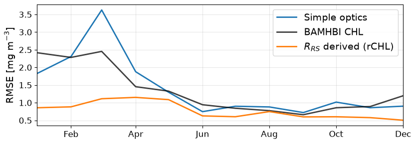
Figure 13 RMSE for chlorophyll over 2018 across the whole basin. Chlorophyll from the simple optics and RT configurations are presented. In the RT configuration, reflectance-derived chlorophyll (R_RS, in orange) is computed following the inversion algorithm used to produce for satellite data in the Black Sea. Chlorophyll from BAMHBI in the RT configuration is shown in black.

4.6 Stochastic model runs

In the stochastic version of the RT model, the optical properties of phytoplankton, non-algal particles and CDOM are perturbed following the experiments described in Macé et al. (2025). We perturb IOPs with first order autoregressive processes with a time correlation of one month and a space correlation of approximately 75 km. The perturbations are defined with a standard deviation of 50 % for absorption and scattering by phytoplankton and non-algal particles, as in Garnier et al. (2016) for the perturbation of biogeochemical parameters. We use a standard deviation of 50 % for the CDOM reference absorption profile a_ref based on the collection of CDOM profiles gathered from BGC-Argo floats described in Appendix A. The standard deviation for the slope S_cdom is taken at 30 % according to the range of values presented in Terzić et al. (2021). For each of the 50 members, we average the reflectances over each month in order to create composites. We compare the outputs of the stochastic configuration of the model with observations from the Galata and Gloria observation towers from the AERONET-OC network (Zibordi et al., 2006, 2009). They provide in situ measurements of water-leaving irradiance close to the western coast of the Black Sea, from which sea surface reflectance is derived. We use data from the Galata platform to compare our reflectance fields over the year 2018 as in the reflectance spectra presented in Fig. 14. In addition to the in situ measurements performed at the Galata station, we also compare it to remote-sensing reflectance provided by the Copernicus Marine Service at the location of the Galata station. We also take advantage of the large dataset provided by this station to explore how the introduction of uncertainties in the RT model is useful when it comes to comparing sea surface reflectance, using the stochastic RT configuration. Figure 14 shows the monthly distribution of the surface spectral reflectance simulated by the stochastic RT module and observed by satellite and at the Galata station. The standard deviation of the ensemble and the extreme values are shown. For observations, values are averaged in each monthly composite and the variability of reflectance within a month is shown using an error bar of one standard deviation length around the average monthly values.

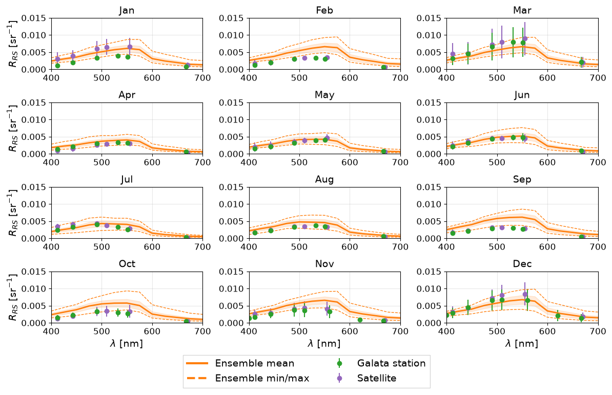
Figure 14 Monthly composites of sea surface reflectance spectra in 2018 at the Galata station (43.045° N, 28.193° E, Romania). Remote-sensing data are taken at the closest grid point to the Galata station. For observations, points represent the average R_RS for the month and bars represent one standard deviation in the data of the month. Model results are taken from the stochastic RT configuration with the ensemble mean in bold lines, the ensemble standard deviation in shaded, and the ensemble minimum and maximum in dotted lines.

In the observations, we notice few differences between the average in situ and remote-sensing data, but rather in the extrema reached, indicating a wider distribution of the data in the remote-sensing product. Therefore, both datasets are rather consistent. The model is able to reproduce the main patterns of R_RS spectra for 2018 in agreement with both sources of data, although some seasonal bias remains. In 2018, in situ data show two early blooms in January and March that are both picked up by the model. However, the simulated reflectance remains high in February between the blooms, indicating a potential merging of these blooms in the model, that is unable to separate them. The extrema members of the ensemble are able to get close to the observations, but the ensemble mean does not fully capture the extent of the variability induced by the blooms. In spring and summer, the simulated reflectance is in agreement with the data, with observations falling within one standard deviation of the ensemble mean. In autumn, the ensemble tends to overestimate R_RS with observations falling at the limit of the ensemble spread, but outside of one standard deviation. The agreement becomes good again at the end of the year with observations close to the ensemble mean in December. The model also represents the gradual increase in reflectance from October to December. The maximum of reflectance is observed around 550 nm, in agreement with both datasets.

5 Discussion

We present a spectral RT model that simulates the propagation of irradiance along the upward and downward vertical directions in three streams. The main outputs of the RT model are the spectral irradiances and the sea surface reflectance, which are quantities measured by radiometric sensors onboard satellites, BGC-Argo floats, and coastal stations. It links simulated variables and observations of sea surface reflectance, avoiding the use of uncertain inversion algorithms. To perform this study, we use the model described in Dutkiewicz et al. (2015) without changing its main features. Some additional changes could be brought to the model without major consequences for the current applications. First, the scattered stream of irradiance E_s does not contain any information that is directly comparable with the data sources that we have been using in this study. E_s could only become relevant if scattering in situ data were used in the comparison. For the comparison with remote-sensing data, this stream could be removed from the model in its future iterations. Then, the definition of IOPs could be further updated. We have already adapted the method for the computation of absorption and scattering by non-algal particles and CDOM to the Black Sea use case. We could also imagine the inclusion suspended minerals (SPM) that could be particularly relevant in the sediment charged waters close to river mouths. SPM aggregates suspended particles of organic and inorganic origin, and we would expect its contribution to be larger in longer wavebands (Grégoire et al., 2023). In the current formulation, model parameterisation is made such as the organic part of SPM is accounted for in the optical properties of non-algal particles. The missing contribution is also compensated in the optical properties of CDOM, as they are derived from other contributions. The explicit addition of SPM would require further model parameterisation; including aggregation, and recalibration of the non-algal particles and CDOM contributions.

The RT model is integrated into the NEMO hydrodynamical model, where it is used in the computation of temperature since the heat source in the energy conservation equation is taken from the simulated irradiance streams. The vertical propagation of the spectral irradiance is governed by the seawater IOPs that determine the amount of light that is absorbed and scattered in the forward and backward directions. The water IOPs need to be provided to the RT model, either from a coupled biogeochemical model or from external datasets. The origin of IOP data is here critical as their definition is also a major challenge when working with such a model. Many assumptions introduce uncertainties at different levels. The definition of PFTs is already a strong assumption as it lumps phytoplankton species within few groups, that share the same properties. The optical properties for such groups vary with the species (size, chlorophyll content) and with basins. As such, the use of specific absorption and scattering properties based on studies performed in other basins might be an obstacle to the proper representation of optical properties in the Black Sea. Since these coefficients play a major role in the simulation of irradiance streams, their importance of their definition is paramount.

The RT model and its stochastic version are tested in the Black Sea where they are coupled with NEMO and the biogeochemical model BAMHBI. The quality of the simulated radiometric variables, along with temperature and chlorophyll, is assessed through comparison with satellite and BGC-Argo data. The modelling of in-water irradiance is very consistent with observations, showing low to moderate bias and a high correlation, as demonstrated in Fig. 4 and Table 2. We notice stronger absorption in the model than in the observations for irradiance streams in shorter wavebands, especially close to the surface. As such, more irradiance is absorbed by the surface waters which may contribute to the increased SST observed in the model. In shorter wavebands, CDOM is the main contributor to irradiance absorption. This gap in absorption may indicate that CDOM absorption is too high, and that the forcing created for this work could be improved for surface waters. The quality of the simulated surface chlorophyll is improved by substituting the RT model with a mean error slightly lower over the basin, as represented in Fig. 13. We note a slight improvement in the simulation of E₀ as in Fig. 5, which is consistent with the good representation of irradiance streams. SST performances are slightly degraded with the RT model and the feedback on temperature (Fig. 6), while remaining in an acceptable range of error when compared to in situ data. It is important to note that this change does not significantly influence stratification in the model, thus preserving the main hydrodynamical features of the basin in the simulation.

The RT model explicitly simulates spectral radiometric quantities, enriching the modelling capabilities of the coupled model by providing spectral irradiance and sea surface reflectance. This is a key milestone towards comparison between simulation outputs and remotely-sensing products. In general, comparisons are performed using remote-sensing surface chlorophyll products that require the use of inversion algorithms (e.g. Kajiyama et al., 2018). Such algorithms tend to come with uncertainties, as they extrapolate from limited data onto larger basins. They also reduce the initially rich datasets of reflectance into a single surface chlorophyll estimate. The simulation of sea surface reflectance is a first step toward the direct simulation of what is observed by satellites. Figures 8–10 show that the model is able to capture the main seasonal patterns of sea surface reflectance, but still have localised errors, in particular in blooming conditions. At longer wavelengths such as 670 nm (Fig. 10), where water and non-algal particles dominate the optical properties, the simulated distributions of irradiance are more consistent with observations. This waveband is particularly interesting as it is less commonly used in ocean colour algorithms than blue or green wavebands. It is a waveband where the contribution of particles is dominant, thus highlighting the contribution of this constituent.

We then notice seasonal patterns in the distributions of reflectances at 490 and 555 nm. Between August and December, which corresponds to the period of low biological activity, the agreement between simulated and observed distributions is good, showing that the model is able to simulate reflectances in a consistent way outside of blooming conditions. In this period, we can validate to some extent the parameterisation of optical properties of CDOM and particles. Early in the year, between January and March, simulated reflectances are less spread out than remote-sensing reflectances. The model is not able to capture extremes in reflectances and even tends to overestimate reflectances in March and April, after the spring bloom. Then, the coccolithophore bloom that causes high reflectances at 490 nm between May and July is missing in the model, with distributions that are shifted towards the lower reflectances. This pattern is also visible at 555 nm at a lower magnitude.

The simulation of reflectances also allows us to mimic inversion algorithms by using them on the simulated fields. As such, it provides a relevant framework for estimating uncertainties associated with surface chlorophyll, both in the model and in the satellite products. More generally, we gain information and a better representation of optics through the simulation of reflectances. However, it is subject to the same limitations in the quality of the remote-sensing signal. In the case of large uncertainties on the absorption and scattering coefficients, the comparison can become arbitrary in the same way it can happen in the case of mismatches with the biogeochemical model when using inversion algorithms. A stochastic version of this RT model that accounts for the uncertainties in the IOPs is also provided to estimate the uncertainties that originate from the coupled model itself, by offering to perturb IOPs. Figure 14 shows reflectance spectra over a year in a coastal setting, exhibiting higher uncertainties during blooms. In such periods, such as in December or March, we notice that the uncertainty with the remote-sensing data is also high, sometimes of higher magnitude than model uncertainty. Further analyses would be required to extend the work presented in Macé et al. (2025) on the propagation of uncertainties within the modelling framework to carefully evaluate the relative importance of uncertainties in the data and in the model, but these initial results hint at the new capabilities offered by the simulation of reflectances in the model.

The modelling of sea surface reflectance opens the way towards the direct assimilation of radiometric data. In general, surface chlorophyll is the satellite product assimilated in biogeochemical models (e.g. Santana-Falcón et al., 2020), with in situ data such as BGC-Argo profiles also assimilated in studies (e.g. Teruzzi et al., 2021). There have been first attempts to assimilate optical properties (e.g. Ciavatta et al., 2014) or reflectance data (e.g. Jones et al., 2016) that show promising results. Given the complex relationship between reflectances and other biogeochemical variables, approaches such as Ensemble Kalman Filter (EnKF) seem appropriate as they aim at directly representing cross-covariances. The stochastic version of the RT model is particularly relevant in this context as it provides a tool to estimate model uncertainty, which is critical information for data assimilation. The estimation of uncertainties in the outputs of the RT model has already been discussed in Macé et al. (2025), where ensemble simulations were run to evaluate the consequences of the introduction of uncertainties in the IOPs. Other sources of uncertainty in the fully coupled modelling framework would have to be evaluated, such as the many empirical parameters used in biogeochemistry or the intrinsic model variability. Other methods are being evaluated for uncertainties such as the use of neural networks to estimate the distribution of IOPs by inverting the RT equation, as in Soto López et al. (2025). A combination of different approaches could be explored in the future, for instance, with this method being used to quantify the sources of uncertainty and ensemble modelling being used to evaluate the propagation of uncertainties in the RT model.

The use of the RT model significantly increases the computation time within the NEMO framework. RT is computed individually at each time step, each waveband and for each ocean water column in the model. We find that the computation time is approximately doubled with 33 wavebands compared to the simple optics configuration. While this may not be an issue for short runs that span a couple of years in regional configurations, the inclusion of this RT model becomes costly for long-term simulations, global or high-resolution runs, in particular if ensembles are simulated. The computation time could be reduced by reducing the spectral resolution or by only considering backscattering and not forward scattering, thus simplifying Eqs. (1)–(3). In the configuration used for the test case, it is necessary to run the RT model at each time step because of the connections to hydrodynamics and biogeochemistry in the computation of temperature and E₀. However, users interested in simulating sea surface reflectance with a more simple one-way coupled configuration could run it less often to provide the desired outputs. Despite the increased computation time, the use of this system is relevant for modelling spectral irradiance and reflectance in specific wavebands to focus on water constituents.

6 Conclusion

In this paper, we propose a module to represent marine optics and RT in the NEMO framework, based in large part on the model described in Dutkiewicz et al. (2015). As such, it can be coupled to any biogeochemical model that is itself coupled with NEMO. This model simulates three streams of irradiance with improved spectral resolution, constituting a tool for simulating in-water irradiance and sea surface reflectance. These variables are particularly relevant for model calibration and validation, as it unlocks access to a large amount of both in situ and remote-sensing data. It also complements the simulation of biogeochemical variables by providing optical quantities that are more closely related to products such as satellite surface chlorophyll. A stochastic version of the RT model is also provided as a tool to evaluate uncertainties in the IOPs and their influence on the simulation of radiometric fields.

We use our RT module with the NEMO-BAMHBI modelling framework for the Black Sea, upgrading its capabilities by enabling the simulation of radiometric variables. It is an important development in the context of operational oceanography, as the NEMO-BAMHBI system is used by the Copernicus Marine Service to predict the Black Sea biogeochemistry. The RT model is fully coupled with the physical and biogeochemical components of the model, following extensive calibration of the feedback loops for the simulation of temperature and primary production. The inclusion of this new RT scheme maintains the simulation of physics and biogeochemistry, while providing enriched information on spectral irradiance, which is directly used for the computation of E₀. The comparison with sea surface reflectance from remote-sensing data reveals that the module is able to simulate the main seasonal and spatial patterns in the basin. It complements the biogeochemical variables in providing information on blooms. At this stage, some features are still not captured or remain poorly represented in the model. This leaves room for improvement in our ability to model bio-optics in the Black Sea, by building on top of the present work.

The improved spectral resolution of the RT model opens new perspectives in line with algorithms that have been used to derive biogeochemical products from remote-sensing reflectances. The products of surface chlorophyll or suspended particulate matter, for instance, rely on specific wavebands that have to be modelled to truly match model outputs with the datasets that are provided. The recent hyperspectral missions PACE (NASA) and PRISMA (Italian Space Agency) are now providing reflectance data at very high resolution, and models that are able to increase their spectral resolution will also be valuable to make the most of hyperspectral data (Chowdhary et al., 2019). By gathering data on a much larger number of wavebands, new algorithms could be developed to better dissociate the water constituents. More generally, this opens up further possibilities for the assimilation of reflectance data.

Appendix A: Model calibration using a 1D test model

We first used a 1D test model to calibrate the three-stream RT model that is coupled with the NEMO-BAMHBI system, using the radiative transfer scheme with BGC-Argo data. This version of the model is fast and efficient computation-wise, allowing to easily compute single profiles of irradiances E_d, E_s, and E_u, as well as sea surface reflectance for a single waveband. It does not include any original or significant model development as it is a simple transcription of the existing model presented in Dutkiewicz et al. (2015) into a Jupyter Notebook environment. This notebook is provided with this article as an additional tool that can be used to easily simulate profiles in a simple 1D and non time-dependent framework (Macé, 2025b). The aim was to keep this testing framework as simple as possible. As inputs, it requires the model parameters defined in Table 1, the absorption and scattering spectra of optically active constituents, and an assumption on phytoplankton composition. By default, it is set as if small flagellates, large flagellates, and diatoms are present in equal proportions. This setting can be changed in the model. The model then needs BGC-Argo data that include chlorophyll and particle backscattering at 700 nm to derive seawater IOPs. The vertical resolution is also defined in the inputs, along with the wavelengths in which the computation should be performed. The surface radiative forcing is taken here from MAR data for the Black Sea, with a sample of these data for 2018 provided with the files. RT is computed for all the profiles of the float within the prescribed time range, and results are displayed for sea surface reflectance along BGC-Argo track, and irradiances and IOP profiles.

We use this simple model to simulate profiles based on BGC-Argo data. BGC-Argo floats are drifting buoys that provide both physical and biogeochemical data by collecting profiles every five to ten days. The calibration of the optical properties of phytoplankton and non-algal particles, as well as CDOM absorption was performed using a collection of test profiles ran with this model. IOPs can be derived from measurements of chlorophyll a, CDOM or backscattering coefficients in available wavebands (typically 700 nm). Some floats additionally provide profiles of PAR and irradiance in selected wavebands. We can therefore use the surface radiation to run our 1D model and evaluate its ability to reproduce the full measured profiles.

By automatising the simulation of the three streams of irradiance over several wavebands and profiles, we are able to evaluate biases in the model formulation or in the estimation of IOPs. Perturbations can also be added to the IOPs in order to find the best representation of the optical properties of seawater. By extension, this process could be repeated with data sources other than BGC-Argo data to increase the representativeness and reliability of the calibration. Since the buoys are drifting, we are unable to perform the simulation for the same location at different times. While it allows to cover a larger domain, it offers limited possibility to cover the temporal variability in optical properties.

In particular, the forcing for CDOM absorption was created using this testing model. We use a collection of 625 profiles from BGC-Argo buoys 6901866 and 6903240, that include profiles of irradiances in three wavebands (380, 412 and 490 nm), chlorophyll, particulate backscattering coefficient at 700 nm and CDOM. The profiles considered for this calibration were measured between June 2015 and July 2022. The objective of this calibration was to derive the contribution of CDOM to radiation attenuation in the reference waveband λ_ref=412 nm. Each contribution to absorption is derived according to the following protocol:

• Absorption by seawater is constant and directly known from the model forcing.

• Absorption by phytoplankton is derived from the absorption spectra (see Fig. 1) and chlorophyll concentrations from BGC-Argo profile. As we cannot discriminate between PFTs using BGC-Argo data, we assume here that chlorophyll is equally distributed among them.

• Absorption by particles is derived from backscattering coefficients at 700 nm and the absorption spectra in Fig. 1.

• An optimisation loop runs with CDOM absorption as the unknown to match the downwelling irradiance profile at 490 nm. The shape of the CDOM absorption profile is constrained by the shape of the CDOM profile from BGC-Argo, as described in Sect. 3.1.

This protocol provides a CDOM absorption profile for each BGC-Argo profile. We associate each a_cdom value to the time of the year and sea water density and interpolate it to cover the whole year and range of seawater densities commonly found in the Black Sea. The resulting forcing is presented in Fig. 2.

Appendix B: Code organisation and model versions

The up-to-date NEMO-BAMHBI, which does not include the three-stream RT module, can be found on the public Gitlab of the MAST group from the university of Liège (Vandenbulcke and Grailet, 2025). The code for the version of BAMHBI with which the three-stream radiative transfer model has been coupled is provided in the Zenodo archive (see data availability section: Macé, 2025a). The code for radiative transfer can be found in the MY_SRC/METEO directory and is split into three files:

1. radtrans.F90 contains the main functions for the computation of RT.

2. radtrans_params.F90 contains the input of parameters for the computation of RT.

3. traqsr.F90 contains the temperature scheme for the coupling with NEMO, as defined in Sect. 2.2.

The parameters for using the RT module must be defined in the namelist_cfg file, in the nam_RADTRANS namelist. The parameters to be set there are as defined in Sect. 3.3. In addition, the coupling from the RT module towards NEMO for the computation of temperature has to be activated by setting the flag ln_qsr_RT = .true. in the namtra_qsr namelist. The GEO_LR directory then hosts the absorption and scattering spectra that are necessary to compute RT in the spectra_water.dat, spectra_particles.dat, spectra_plankton.dat, and cdom_sinusoidal.dat files. The surface radiative forcing is taken from the MAR configuration, for which all the data are not made available because of the large size of the dataset. Any atmospheric output containing direct and diffuse radiation is compatible with this configuration.

When the RT module is coupled with BAMHBI, concentrations of the three PFTs and of POC are taken to derive seawater IOPs. Information on water density is taken directly from NEMO to derive CDOM absorption. Then, the irradiance streams are used to compute E₀ that is fed back into the biogeochemical model within the UpdateLight routine of the BAMHBI/bamhbi.F90 file. In the case where the user only wants to use the three-stream RT module as an observation operator and keep using another RT scheme to derive E₀ and temperature, another scheme must be defined in the BAMHBI/bamhbi.h90 file to compute E₀. For physics, another scheme must be chosen (consistent, if possible) in the namtra_qsr namelist.

The radiometric outputs are defined in the traqsr.F90 source file. They can include sea surface reflectance and irradiance streams in relevant wavelengths (i.e. typically those that are measured by satellite sensors of in situ stations). In addition, the ln_radtrans_diags flag is defined in the nam_RADTRANS namelist to output secondary variables such as IOPs or their decomposition by optically active constituent. The output field and file structures must then be defined accordingly for each experiment.

The RT module can also be used without coupling a biogeochemical model. In this case, the nam_RADTRANS_inputs namelist is used to provide external data of chlorophyll and POC concentrations. Together with the absorption and scattering spectra, they are used to derive seawater IOPs. In this configuration, the computation of absorption by CDOM remains unchanged and is derived from the seawater density that is computed in NEMO.

When using the stochastic version of the model, the inputs for perturbations (standard deviations, temporal, and spatial correlations) must be provided in the namsto namelist. When perturbations are activated, they are applied during the computation of the RT scheme, of which the code is located in the radtrans.F90 file.