DIRECT 1.0: a diffusion-based generative model for dense sea surface temperature reconstructions from sparse satellite observations

Satellite sea surface temperature (SST) observations are frequently obscured by cloud cover, creating large gaps that must be reconstructed for many oceanographic and climate applications. Because multiple high-resolution SST fields may be consistent with the same sparse observations, this reconstruction problem is inherently ambiguous. Nevertheless, most existing approaches remain deterministic, producing a single estimate that is often overly smooth, may contain unrealistic artifacts, and provides limited or unreliable uncertainty estimates. To address these limitations, we introduce DIRECT, a conditional generative framework for dense SST reconstruction that models the full distribution of plausible solutions rather than a single deterministic estimate. DIRECT is based on a rectified flow-matching formulation, conditioned on temporal context and day-of-year seasonality, and trained on sparse Level-3 observations. It presents an observation-guided rectification that anchors the generative trajectory to measured pixels at every integration step. By sampling multiple reconstructions, DIRECT produces an ensemble of physically plausible SST fields, enabling both an accurate mean reconstruction and spatially resolved uncertainty estimates. The latter is adjusted with a simple post-hoc variance term to avoid under-dispersed uncertainty estimates. Experiments on three Level-3 SST datasets (Mediterranean, Adriatic, and Atlantic) show that DIRECT sets a new state-of-the-art, reducing Root Mean Square Error by 6 %–14 % compared with the strongest published method, while better preserving mesoscale structure. Further analysis of spatial scale correlations indicates that DIRECT maintains physically consistent textures even when reconstructing large, completely unobserved regions. Performance improvements remain robust across a wide range of cloud-coverage conditions, enabling reliable SST reconstruction from sparse satellite observations.

1 Introduction

Sea surface temperature (SST) is a key variable at the ocean–atmosphere interface, regulating exchanges of heat, moisture, and momentum and influencing atmospheric convection, storm development, and large-scale climate variability such as ENSO and monsoon systems (Rahman and Rahaman, 2024; Li et al., 2024; Garcia-Soto et al., 2021; Ricchi et al., 2023). SST is therefore recognized as an essential climate variable (Bojinski et al., 2014) and is widely used in climate monitoring, numerical weather prediction, ocean reanalysis, and marine ecosystem studies (Senatore et al., 2020; Donlon et al., 2007).

Global SST observations are primarily obtained from satellite-based infrared (IR) and microwave radiometers on low-Earth-orbit and geostationary platforms (O'Carroll et al., 2019). IR instruments provide fine spatial detail, but their usable coverage is strongly limited by clouds. At a given time, cloud systems can hide large coherent areas of the ocean surface, resulting in structured gaps that persist across space and time. These gaps present a challenge for downstream applications that require spatially complete SST fields (climatological datasets, surface boundary conditions for atmospheric models, etc.).

Early SST reconstruction methods based on statistical interpolation and low-rank decompositions (e.g., Optimal Interpolation, EOFs, Taburet et al., 2019; Alvera-Azcárate et al., 2005) recover large-scale variability but are limited in representing fine-scale and nonlinear ocean dynamics, due to linearity and stationarity assumptions. Recent learning-based methods have substantially improved reconstruction quality by exploiting spatial and temporal correlations in the data. Convolutional autoencoders such as DINCAE/DINCAE2 (Barth et al., 2020, 2022) provide uncertainty surrogates but often produce overly smooth fields and underestimate mesoscale variability. Transformer-based architectures, including MAESSTRO (Goh et al., 2024) and CRITER (Zupančič Muc et al., 2025), improve the modeling of long-range dependencies but remain fundamentally deterministic, producing a single best-guess reconstruction that struggles to capture ambiguity under heavy cloud cover, complicates uncertainty estimation, and may introduce unrealistic structured artifacts (Fig. 1, bottom-right).

In machine learning, particularly in computer vision, diffusion-style generative models have achieved state-of-the-art performance in image restoration by learning full conditional distributions rather than point estimates (Croitoru et al., 2023; Li et al., 2023; Xing et al., 2024). Pixel re-injection as in RePaint (Lugmayr et al., 2022) and subsequent refinements (Liu et al., 2024) has been successfully exploited to enforce observation consistency during sampling for inpainting. However, these methods typically operate on single images and do not address spatiotemporally structured gaps, physical masks (e.g., land), or calibrated uncertainty in geophysical fields. A growing body of work applies diffusion-style generative models to Earth-science reconstruction tasks. Barth et al. (2024) demonstrate diffusion-based gap-filling for satellite ocean color (chlorophyll a), producing ensembles and evaluating uncertainty reliability. For SST specifically, CARE-SST (Choo et al., 2025) applies a denoising diffusion probabilistic model (DDPM, Ho et al., 2020) style approach with historical context to reconstruct cloud-contaminated SST. Related efforts also extend diffusion-based reconstruction to broader ocean-temperature settings using observation-guided sampling and simulation pretraining (Song et al., 2025). In atmospheric data assimilation, physics-guided diffusion frameworks incorporate physical regularization to improve coherence under sparse observations (Wang et al., 2025). Two concurrent studies extend this direction to global, climate-scale reconstruction: Qian et al. (2026) pretrain a spatiotemporal diffusion prior on climate-model simulations and reanalysis to reconstruct monthly historical temperature and precipitation fields from sparse instrumental records, while Li et al. (2026) perform diffusion posterior sampling to fuse coarse-resolution microwave retrievals with sparse in situ measurements into global ensemble SST estimates. While these works establish promise of generative modeling for geosciences, a crucial difference to the work presented in this paper is that they operate on a single shot or coarse temporal context (Choo et al., 2025; Qian et al., 2026), rely on guidance schemes without explicit temporal encoding (Song et al., 2025; Li et al., 2026), require gap-free training data (Qian et al., 2026; Choo et al., 2025) and do not target calibrated per-pixel uncertainty for dense spatiotemporal reconstruction (Wang et al., 2025).

In this study we propose DIRECT, a diffusion-inspired generative model for dense SST reconstruction from partially observed sparse satellite measurements. DIRECT formulates SST gap-filling as a conditional flow-matching task (Lipman et al., 2023), where a deterministic probability flow transforms noise realizations into physically consistent SST fields conditioned on sparse measurements, temporal context, and seasonal information. The model integrates (i) a backbone equipped with SST-specific global conditioning, (ii) a spatio-temporal context representation that preserves the temporal origin of auxiliary information, and (iii) an observation-guided rectification mechanism that maintains consistency with measured pixels throughout the reconstruction process. By sampling multiple reconstructions, DIRECT produces both an accurate mean estimate and spatially resolved uncertainty, which is further automatically calibrated to avoid ensemble collapse. The main contributions are:

• We formulate dense SST reconstruction as a conditional flow-matching problem, integrating spatiotemporal context, seasonal conditioning, and hard observation consistency within a unified end-to-end generative model.

• We develop a temporal offset encoding strategy for auxiliary context frames.

• We design a lightweight post-hoc uncertainty calibration procedure that compensates for ensemble under-dispersion and improves the reliability of per-pixel uncertainty estimates without altering the training objective.

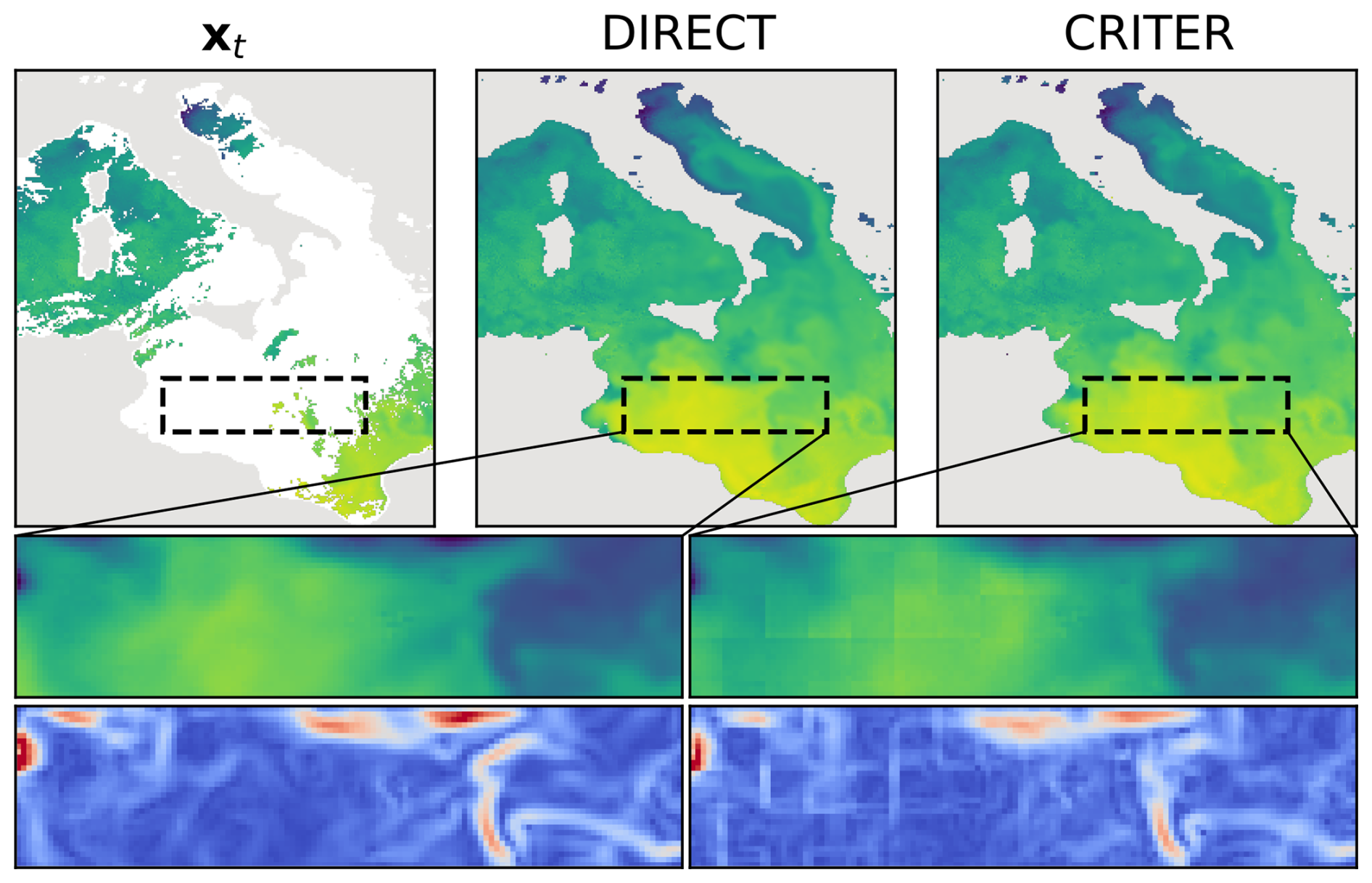
Figure 1 DIRECT reconstructs spatially coherent temperature fields from sparse observation inputs and preserves smooth mesoscale structure in reconstructed regions. DIRECT further addresses the problem of physically inconsistent reconstructions – notice that the blocky high-frequency gradients emerging in CRITER (Zupančič Muc et al., 2025, bottom right), which are absent in DIRECT reconstructions (bottom left).

A preliminary version of this work was presented in Rovšček et al. (2026), which the present work extends in several ways. The reconstruction method has been revised following extended evaluation under operationally realistic conditions, resulting in a simpler and more robust formulation. The experimental evaluation is broadened to include an additional state-of-the-art baseline (CARE-SST, Choo et al., 2025), a stratified performance analysis across low, moderate, and high cloud-coverage regimes, and a probabilistic assessment of the reconstructed ensemble via the Continuous Ranked Probability Score. Additionally, a series of new ablation studies examines the individual contributions of seasonal context, mask-aware conditioning, temporal encoding design, and future context availability for near-real-time operational applications.

2 DIRECT architecture and implementation

We begin by introducing key notations and definitions. Let $\mathbf{X}=\mathit{\{}{\mathit{x}}_{\mathrm{1}},{\mathit{x}}_{\mathrm{2}},\mathrm{\dots }{\mathit{x}}_T\mathit{\}}=\mathit{\{}{\mathit{x}}_t{\mathit{\}}}_{t=\mathrm{1}}^T$ denote a sequence of SST measurements ${\mathit{x}}_t\in {\mathbb{R}}^{W\times H}$, and $\mathbf{M}=\mathit{\{}{\mathit{m}}_t{\mathit{\}}}_{t=\mathrm{1}}^T$ a sequence of corresponding binary masks ${\mathit{m}}_t\in \mathit{\{}\mathrm{0},\mathrm{1}{\mathit{\}}}^{W\times H}$, with ones indicating valid observations, and let m_l be a constant binary mask, with zeros indicating land. Our task is to recover a sequence of dense (gap-free) reconstructed fields $\mathit{\{}{\mathit{\mu }}_t{\mathit{\}}}_{t=\mathrm{1}}^T$ along with per-pixel uncertainty estimates $\mathrm{\Sigma }=\mathit{\{}{\mathit{\sigma }}_t{\mathit{\}}}_{t=\mathrm{1}}^T$. Here, W denotes the width and H the height, in pixels, of the SST frame.

Reconstructing SST fields is fundamentally a spatio-temporal inference task because ocean surface temperatures evolve continuously under physical constraints. Consequently, measurements acquired close in time to day t are typically informative for recovering missing values, whereas observations from more distant times tend to contribute less. Previous work (Barth et al., 2022; Zupančič Muc et al., 2025) showed that most relevant temporal information is contained within a three-day window centered at the target frame. Following these findings, we use observations from days t−1, t, and t+1 when reconstructing missing regions at time t.

Because adjacent context frames may themselves be partially observed, we densify the temporal context by opportunistically replacing missing pixels with observations from nearby days. For a pixel that is missing at time t−1, we use the closest available observation from t−2 or t−3. Analogously, missing pixels at t+1 are filled from t+2 or t+3. The resulting filled context frames are denoted as ${\mathit{x}}_{t-\mathrm{1}}^{\prime }$ and ${\mathit{x}}_{t+\mathrm{1}}^{\prime }$. Note that this search depth Δ_filled=3 is distinct from the three-day context window, and extends the total temporal footprint of the input to days t−3 through t+3. A value drawn from an earlier day substitutes for the state at t−1 and stays informative only over the timescale on which SST remains temporally autocorrelated, so the same short temporal decorrelation that motivates a narrow context window also bounds the depth over which substitution is meaningful. To retain the temporal origin of each filled value, we associate every context frame with a one-hot encoded mask. For the past context, ${\mathbf{M}}_{t-\mathrm{1}}\in \mathit{\{}\mathrm{0},\mathrm{1}{\mathit{\}}}^{\mathrm{3}\times W\times H}$ encodes whether a pixel originates from day t−1, t−2, or t−3. For the future context, ${\mathbf{M}}_{t+\mathrm{1}}\in \mathit{\{}\mathrm{0},\mathrm{1}{\mathit{\}}}^{\mathrm{3}\times W\times H}$ similarly encodes offsets t+1, t+2, or t+3. Since each pixel is filled from the temporally nearest valid frame, these channels are mutually exclusive, while a null vector $[\mathrm{0},\mathrm{0},\mathrm{0}]$ denotes a pixel that remains invalid (land or persistent cloud cover) after the search. The central frame is represented by a two-channel mask ${\mathbf{M}}_t\in \mathit{\{}\mathrm{0},\mathrm{1}{\mathit{\}}}^{\mathrm{2}\times W\times H}$, which distinguishes observed from missing (or land) pixels at time t. We define the temporal context fields as ${\mathbf{C}}_{\mathrm{1}t}=[{\mathit{x}}_{t-\mathrm{1}}^{\prime },{\mathit{x}}_t,{\mathit{x}}_{t+\mathrm{1}}^{\prime }]$ and the corresponding masks as ${\mathbf{C}}_{\mathrm{2}t}=[{\mathbf{M}}_{t-\mathrm{1}},{\mathbf{M}}_t,{\mathbf{M}}_{t+\mathrm{1}}]$, whose construction for a general search depth is summarized in Algorithm 1. Together, these form the complete spatio-temporal context ${\mathbf{C}}_t=({\mathbf{C}}_{\mathrm{1}t},{\mathbf{C}}_{\mathrm{2}t})$. Following good practices of prior work (Barth et al., 2022; Zupančič Muc et al., 2025), we additionally include the day-of-year (DoY) d_t as seasonal context information. Figure 2 shows an example of context information.

Algorithm 1 Temporal context construction for target day t. The accumulator f marks pixels that have already been assigned a temporal origin, and s_j marks pixels filled from offset j. Because s_j is nonzero only where f=0, the origin channels are mutually exclusive by construction.

Input:

SST sequence X, mask sequence M, target day t, search depth Δ_filled

Output:

context fields C_1t, temporal-origin masks C_2t

1:

Past context:

2:

${\mathit{x}}_{t-\mathrm{1}}^{\prime }\leftarrow \mathbf{0}$,  f←0

3:

for j=1 to Δ_filled do

4:

${\mathit{s}}_j\leftarrow {\mathit{m}}_{t-j}\odot (\mathrm{1}-\mathit{f})$ {pixels first filled from day t−j}

5:

${\mathit{x}}_{t-\mathrm{1}}^{\prime }\leftarrow {\mathit{x}}_{t-\mathrm{1}}^{\prime }+{\mathit{x}}_{t-j}\odot {\mathit{s}}_j$

6:

${\mathbf{M}}_{t-\mathrm{1}}\left[j\right]\leftarrow {\mathit{s}}_j$

7:

$\mathit{f}\leftarrow \mathit{f}+{\mathit{s}}_j$

8:

end for

9:

Future context: ${\mathit{x}}_{t+\mathrm{1}}^{\prime },{\mathbf{M}}_{t+\mathrm{1}}\leftarrow$ as above, with x_t+j and m_t+j

10:

Central frame:

11:

M_t[1]←m_t {observed}

12:

${\mathbf{M}}_t\left[\mathrm{2}\right]\leftarrow \mathrm{1}-{\mathit{m}}_t$ {missing or land}

13:

${\mathbf{C}}_{\mathrm{1}t}\leftarrow [{\mathit{x}}_{t-\mathrm{1}}^{\prime },{\mathit{x}}_t,{\mathit{x}}_{t+\mathrm{1}}^{\prime }]$

14:

${\mathbf{C}}_{\mathrm{2}t}\leftarrow [{\mathbf{M}}_{t-\mathrm{1}},{\mathbf{M}}_t,{\mathbf{M}}_{t+\mathrm{1}}]$

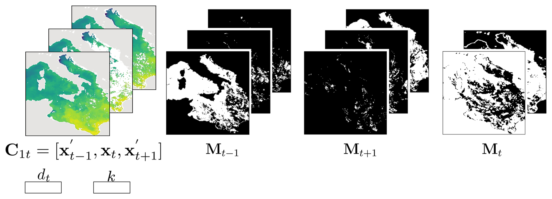
Figure 2 Context information fields provided to DIRECT at input. DIRECT uses a three-day SST window ${\mathbf{C}}_{\mathrm{1}t}=[{\mathit{x}}_{t-\mathrm{1}}^{\prime },{\mathit{x}}_t,{\mathit{x}}_{t+\mathrm{1}}^{\prime }]$, with corresponding one-hot encoded masks M_t−1 and M_t+1 indicating the temporal origin of filled pixels, and M_t marking observed versus missing values in the central frame. Additional conditioning is provided by the day-of-year (d_t) and the flow timestep k.

2.1 A flow-matching architecture

We frame the SST reconstruction as a conditional flow matching problem (Lipman et al., 2023), where the reconstruction trajectory is represented as a deterministic transport from an initial simple noise distribution toward the target data distribution. The process involves simulating a stochastic differential equation, for which the Euler integration at iteration step $k\in [\mathrm{0},\mathrm{1}]$ is

$$\begin{array}{}\text{(1)}& {\widehat{\mathit{x}}}_t^{(k+\mathrm{\Delta })}={\stackrel{\mathrm{̃}}{\mathit{x}}}_t^{\left(k\right)}+\mathrm{\Delta }\cdot {\mathit{v}}_{\mathit{\theta }}\left({\stackrel{\mathrm{̃}}{\mathit{x}}}_t^{\left(k\right)}\right|{\mathbf{C}}_t,k,d_t),\end{array}$$

where Δ is the integration step, ${\mathit{v}}_{\mathit{\theta }}\left({\stackrel{\mathrm{̃}}{\mathit{x}}}_t^{\left(k\right)}\right|{\mathbf{C}}_t,k,d_t)$ is the rectified flow network, with C_t representing the aggregated spatio-temporal context, d_t the day-of-the-year variable, and ${\stackrel{\mathrm{̃}}{\mathit{x}}}_t^{\left(k\right)}$ the previous iteration reconstruction ${\widehat{\mathit{x}}}_t^{\left(k\right)}$ with observed values re-injected via the FUSE operation (Fig. 3), i.e.,

$$\begin{array}{}\text{(2)}& {\stackrel{\mathrm{̃}}{\mathit{x}}}_t^{\left(k\right)}=\text{FUSE}\left({\widehat{\mathit{x}}}_t^{\left(k\right)}\right)=({\widehat{\mathit{x}}}_t^{\left(k\right)}\odot (\mathrm{1}-{\mathit{m}}_{\text{t}})+{\mathit{x}}_t\odot {\mathit{m}}_{\text{t}})\odot {\mathit{m}}_l,\end{array}$$

where ⊙ is the Hadamard (element-wise) product. By re-injecting the clean observations at every step, the learned updates of the network v_θ are restricted only to regions with missing SST values.

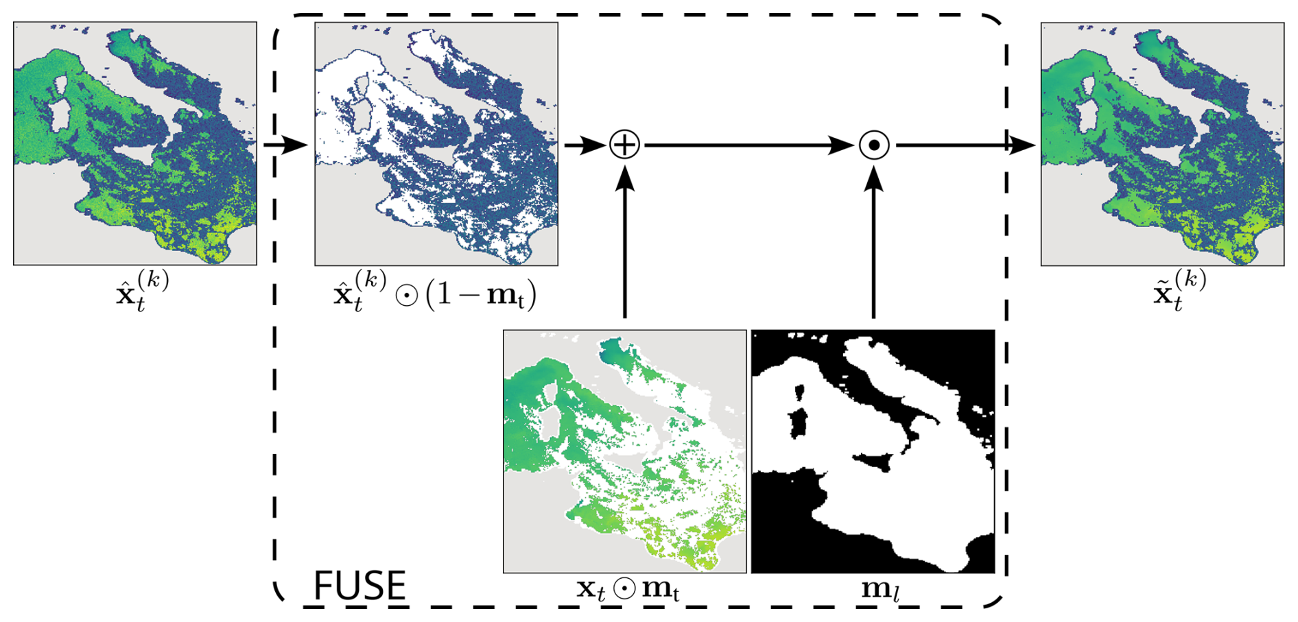
Figure 3 The FUSE operation. At each integration step k, the current estimate ${\widehat{\mathit{x}}}_t^{\left(k\right)}$ is merged with the original observations x_t. This ensures that measured pixels remain preserved (non-corrupted) while the model updates the missing regions.

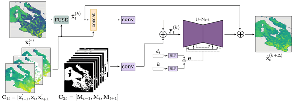
Figure 4 illustrates the architecture of the rectified flow network ${\mathit{v}}_{\mathit{\theta }}\left({\stackrel{\mathrm{̃}}{\mathit{x}}}_t^{\left(k\right)}\right|{\mathbf{C}}_t,k,d_t)$. The current reconstruction state ${\stackrel{\mathrm{̃}}{\mathit{x}}}_t^{\left(k\right)}$ and the temporal SST context C_1t are concatenated and projected into a feature representation through a 1×1 convolution. In parallel, the temporal-origin masks C_2t are independently embedded using a separate 1×1 convolution and subsequently added to the feature tensor. The resulting representation defines the network input ${\mathit{y}}_t^{\left(k\right)}\in {\mathbb{R}}^{\mathrm{128}\times W\times H}$. The backbone follows the U-Net design of (Lipman et al., 2024), where the encoder progressively increases the feature dimensionality across four resolution levels with channel widths (128, 256, 384, 512). The highest-resolution stage uses five residual blocks, while the remaining stages use three residual blocks each. Self-attention is applied only at the lowest spatial resolution.

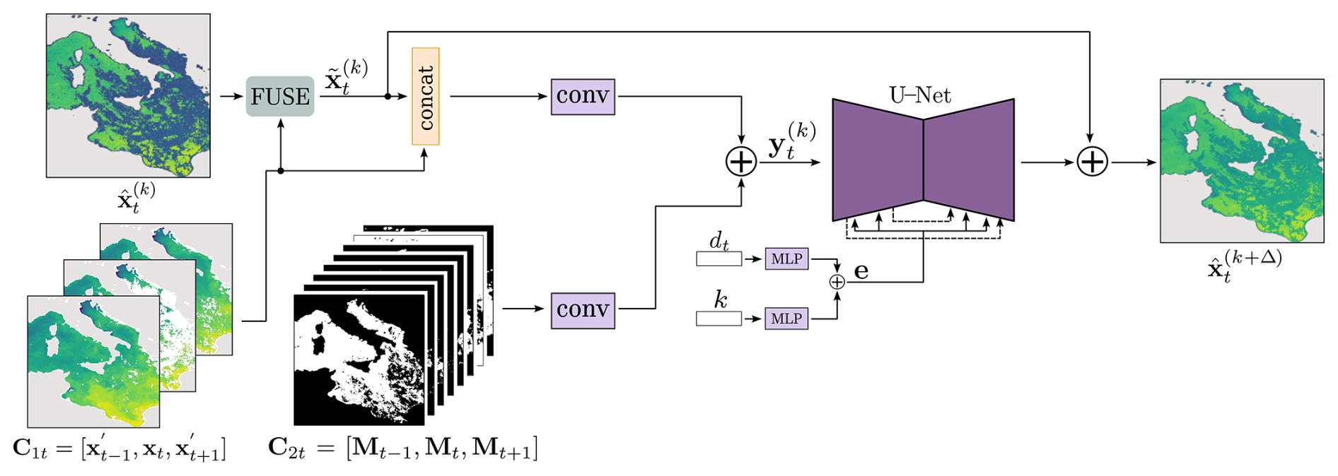
Figure 4 Overview of the DIRECT architecture. The SST field ${\widehat{\mathit{x}}}_t^{\left(k\right)}$ estimated at kth iteration is accompanied by the temporal context C_1t and the time-stamp masks C_2t, seasonal context d_t, and the current flow iteration value k. The FUSE rectified reconstruction ${\stackrel{\mathrm{̃}}{\mathit{x}}}_t^{\left(k\right)}$ is concatenated with context frames C_1t and summed with the embedded origin masks C_2t to form the network input. Token e modulates the U-Net via FiLM (Perez et al., 2018). The network output updated the initial SST estimate into ${\widehat{\mathit{x}}}_t^{(k+\mathrm{\Delta })}$ by Euler integration.

Feature modulation is performed using FiLM conditioning (Perez et al., 2018). A global conditioning vector e∈ℝ⁵¹² is constructed by summing two embeddings: (i) Seasonal information is encoded from the day-of-year variable d_t using its sine-cosine representation $\left[\sin \right(d_t\frac{\mathrm{2}\mathit{\pi }}{\mathrm{365.25}}),\cos (d_t\frac{\mathrm{2}\mathit{\pi }}{\mathrm{365.25}}\left)\right]$, mapped through a two-layer MLP; and (ii) The current flow iteration variable k is encoded separately using sinusoidal embeddings and an additional two-layer MLP. The resulting conditioning token modulates feature maps throughout all residual blocks of the U-Net.

2.2 Probabilistic reconstruction

To obtain probabilistic SST estimates, the reconstruction process is repeated N=16 times using different Gaussian initializations in the missing regions, producing an ensemble of reconstructions $\mathbf{S}=\mathit{\{}{\widehat{\mathit{x}}}_{t,n}{\mathit{\}}}_{n=\mathrm{1}}^N$. Ideally, the ensemble spread should approximate the posterior uncertainty at each pixel. However, we observed that the ensemble variance occasionally becomes under-dispersed at isolated spatial locations. To address this effect, we model the ensemble as a mixture of Gaussians, each centered at ensemble member with a small constant variance ${\mathit{\sigma }}_{\mathrm{0}}^{\mathrm{2}}$ across all pixels. The final reconstruction is thus obtained by moment-matching the mixture with a single Gaussian, i.e.,

$$\begin{array}{}\text{(3)}& {\mathit{\mu }}_t=<\mathbf{S}>;{\mathit{\sigma }}_t^{\mathrm{2}}=\text{var}\left(\mathbf{S}\right)+{\mathit{\sigma }}_{\mathrm{0}}^{\mathrm{2}},\end{array}$$

where the constant ${\mathit{\sigma }}_{\mathrm{0}}^{\mathrm{2}}$ is estimated on the validation set (explained in the next section).

2.3 Training procedure

To enable training with incomplete data, DIRECT is trained by a modified self-supervised flow-matching objective. The training samples are created by sampling cloud masks m_m from other days and applying them to the central day, yielding ${\mathit{x}}_t^{\prime \prime }={\mathit{x}}_t\odot {\mathit{m}}_m$ (Fig. 5). Thus, a ground truth direction vector ${\mathit{u}}_t={\mathit{x}}_t-{{\stackrel{\mathrm{̃}}{\mathit{x}}}^{\prime \prime }}_t^{\left(\mathrm{0}\right)}$ is constructed from the original observed field (x_t) and the simulated observed field with missing values initialized by noise (${{\stackrel{\mathrm{̃}}{\mathit{x}}}^{\prime \prime }}_t^{\left(\mathrm{0}\right)}$). The flow iteration variable k is sampled at uniform from interval [0,1], leading to the following loss at field indexed by time-step t:

$$\begin{array}{}\text{(4)}& {\mathcal{L}}_t={\displaystyle \frac{\mathrm{1}}{N_t}}\sum _{i=\mathrm{1}}^{N_t}\left[{\left({\mathit{v}}_{\mathit{\theta }}\left({\stackrel{\mathrm{̃}}{\mathit{x}}}_t^{\left(k\right)}\right|{\mathbf{C}}_t,k,d_t{)}_{\left(i\right)}-{\mathit{u}}_{t,i}\right)}^{\mathrm{2}}{\mathit{m}}_{t\left(i\right)}\right],\end{array}$$

where $N_t=\left|{\mathit{m}}_t\right|$ is the number of observed pixels in the ground truth SST field. Note that because complete cloud-free data is unavailable, we cannot supervise in the originally clouded regions. As such, this simulation-based approach allows the model to learn the underlying spatial correlations from the available data.

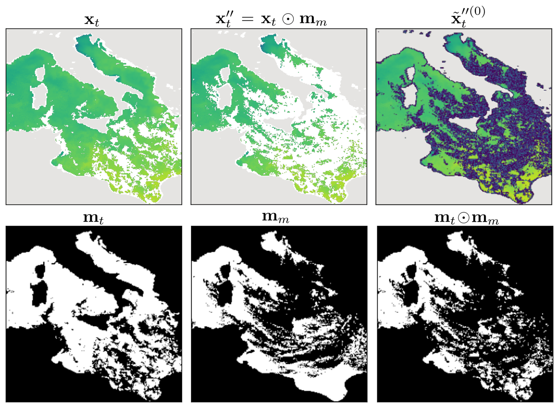
Figure 5 First row: ground truth incomplete central day observation (x_t), simulated central day observation (${\mathit{x}}_t^{\prime \prime }$), noised initialized simulated central day observation (${{\stackrel{\mathrm{̃}}{\mathit{x}}}^{\prime \prime }}_t^{\left(\mathrm{0}\right)}$). Second row: mask denoting valid observations in ground truth observation (m_t), sampled mask from a different day (m_m), mask denoting observed regions in the simulated central day observation (m_t⊙m_m).

After training the model, the training set (or validation if available) can be reconstructed and the regularization variance ${\mathit{\sigma }}_{\mathrm{0}}^{\mathrm{2}}$ estimated as follows. Following (Zupančič Muc et al., 2025) we define per-pixel scaled reconstruction error as

$$\begin{array}{}\text{(5)}& \mathit{ϵ}={\displaystyle \frac{{\mathit{x}}_t-{\mathit{\mu }}_t}{{\mathit{\sigma }}_t}}.\end{array}$$

For a well-calibrated estimator, this error should follow a unit-variance, zero-centered Gaussian, i.e., μ_ϵ→0 and σ_ϵ→1, where μ_ϵ and σ_ϵ are the empirical mean and standard deviation of ϵ, calculated over the training (or validation) set. The regularization variance ${\mathit{\sigma }}_{\mathrm{0}}^{\mathrm{2}}$ can thus be estimated by minimizing the KL divergence (Kullback and Leibler, 1951) between the zero-mean, unit Gaussian and the empirical Gaussian obtained from Eq. (5), which yields the following loss

$$\begin{array}{}\text{(6)}& {\mathcal{L}}_{{\mathit{\sigma }}_{\mathrm{0}}^{\mathrm{2}}}={\mathit{\mu }}_{\mathit{ϵ}}^{\mathrm{2}}+{\mathit{\sigma }}_{\mathit{ϵ}}^{\mathrm{2}}-\log {\mathit{\sigma }}_{\mathit{ϵ}}^{\mathrm{2}}.\end{array}$$

3 Training, Validation and Testing Data

To assess DIRECT, we adopt three datasets corresponding to Mediterranean, Adriatic and Atlantic regions. These regions were chosen because they exhibit very diverse oceanographic regimes. Mediterranean basin contains several characteristic sub-basins, including regions of freshwater influence, frontal systems and regions with submesoscale and mesoscale eddy activity. Adriatic has a shallow shelf in the north, highly influenced by local freshwater discharges, while its southern part is deeper and exposed to Atlantic and Levantine medium waters entering through Otranto strait from the Ionian sea. Finally, the Atlantic region is essentially an open ocean, marked by intense cyclonic activity and cloudiness. All datasets are based on level-3 (L3) multi-sensor SST products and are provided as daily fields remapped onto uniform regular grids. For each dataset, we employ chronological splits to prevent temporal leakage: first 90 % of the samples are used for training, further 5 % are used for validation (to monitor model performance and guide design choices), and final 5 % are used for testing.

1. The Mediterranean SST_MED_SST_L3S_NRT_OBSERVATIONS_010_012 (E.U. Copernicus Marine Service Information, 2024c) dataset consists of daily SST observations over the Central Mediterranean from 1 January 2008 to 31 December 2021, remapped to a 0.0625°×0.0625° grid.

2. The Adriatic SST_MED_PHY_L3S_MY_010_042 (E.U. Copernicus Marine Service Information, 2024a) dataset contains daily SST fields over the Adriatic Sea from 25 August 1981 to 31 December 2022, remapped to a 0.05°×0.05° grid.

3. The Atlantic SST_ATL_PHY_L3S_MY_010_038 (E.U. Copernicus Marine Service Information, 2024b) dataset spans an open-ocean region in the North Atlantic from 1 January 1982 to 1 January 2022, remapped to a 0.05°×0.05° grid.

Following Zupančič Muc et al. (2025), we apply a coverage threshold to the central observation in each input triplet to filter out samples with excessive cloud cover. A sample is discarded if more than a dataset-specific percentage of the central frame is missing: 100 % for the Mediterranean, 60 % for the Adriatic, and 75 % for the Atlantic dataset. After filtering, we obtain 5114 valid samples for the Mediterranean, 7800 for the Adriatic, and 3454 for the Atlantic dataset.

4 Results

4.1 Performance measures

We report the Root Mean Squared Error (RMSE) calculated over three specific regions: the region with observed data (RMSE_obs), the region in which we occluded the data (RMSE_mis), and the two regions combined for overall evaluation (RMSE_all). While RMSE_obs is included for completeness, it is not particularly informative: due to the FUSE rectification step (Eq. 2), observed pixels are replaced with their measured values at every flow integration step, leading to near-zero error. Nevertheless, note that many competing methods also reconstruct this part of the data, necessarily increasing the errors also in the observed regions. The metric of primary interest is therefore RMSE_mis, which reflects the quality of reconstruction in the occluded regions.

4.2 Comparison with state-of-the-art

DIRECT is evaluated against four recent SST reconstruction approaches: DINCAE2 (Barth et al., 2022), CARE-SST (Choo et al., 2025), MAESSTRO (Goh et al., 2024), and CRITER (Zupančič Muc et al., 2025). We follow the evaluation procedure introduced by Zupančič Muc et al. (2025), in which each test sample is evaluated under 10 independently sampled cloud-mask realizations applied to the central frame. Final performance scores are obtained by averaging the reconstruction errors across all repetitions and all samples in the test dataset.

Results in Table 1 show that across all three datasets, DIRECT achieves the lowest reconstruction error among all considered methods. Relative to DINCAE2, DIRECT reduces RMSE_mis by 52 % on the Adriatic dataset, 27 % on the Mediterranean, and 7 % on the Atlantic dataset. Improvements over MAESSTRO are even greater, ranging from 41 % on the Atlantic to more than 62 % on both the Mediterranean and Adriatic datasets. Notably, because CARE-SST was originally designed for fully-observed ground truth, we adapted its training objective to our self-supervised formulation (Sect. 2.3) to enable learning from incomplete data. Even with this adaptation, DIRECT achieves RMSE_mis by 55 % lower on the Mediterranean, 51 % on the Adriatic, and 36 % on the Atlantic. Compared to CRITER, the strongest published baseline, DIRECT further reduces reconstruction error in occluded regions by 14 % on the Adriatic, 8 % on the Mediterranean, and 6 % on the Atlantic. The quantitative improvements are also reflected in the spatial consistency of the reconstructed SST fields. Figures 6, 7, and 8 show DIRECT and CRITER reconstruction examples from the Mediterranean, Adriatic, and Atlantic datasets, respectively. Across the Mediterranean and Adriatic examples, DIRECT better recovers the underlying SST structure under a wide variety of cloud shapes and coverage levels. For the Atlantic domain, where cloud cover is typically more extensive and ocean variability more energetic, CRITER reconstructions often exhibit visible patch artifacts, a byproduct of its patch-based processing. DIRECT avoids such artifacts due to its fully convolutional diffusion backbone and produces more spatially consistent fields even under extreme occlusions. For additional figures refer to Appendix A. For subsequent experiments, we retain CRITER as the sole baseline, since it consistently outperforms DINCAE2 and MAESSTRO.

(Goh et al., 2024)(Choo et al., 2025)(Barth et al., 2022)(Zupančič Muc et al., 2025)(Goh et al., 2024)(Choo et al., 2025)(Barth et al., 2022)(Zupančič Muc et al., 2025)(Goh et al., 2024)(Choo et al., 2025)(Barth et al., 2022)(Zupančič Muc et al., 2025)

Table 1 Comparison of DIRECT to current state-of-the-art methods. All of the reported reconstruction errors are in °C, where the two numbers in parentheses correspond to the 10 % and 90 % percentiles. Bold indicates the best result per column within each dataset.

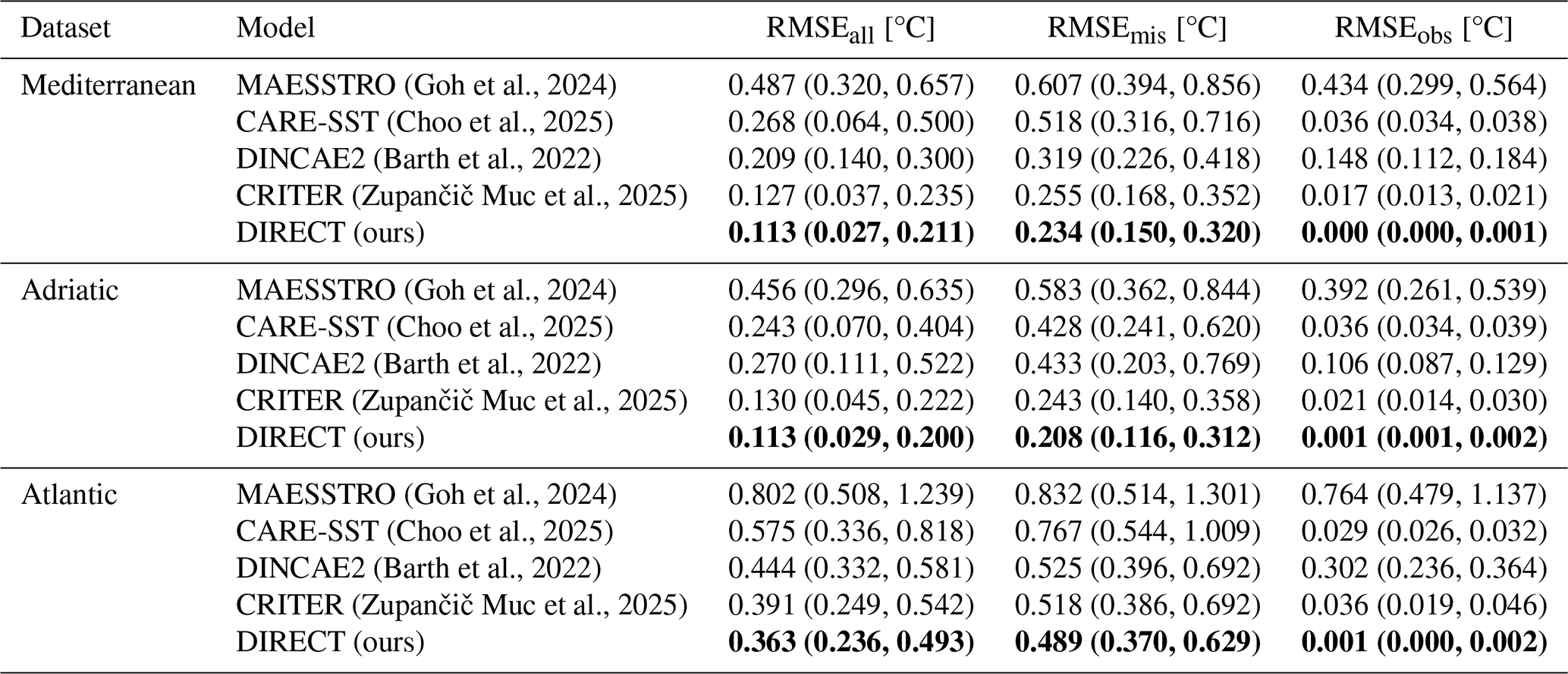
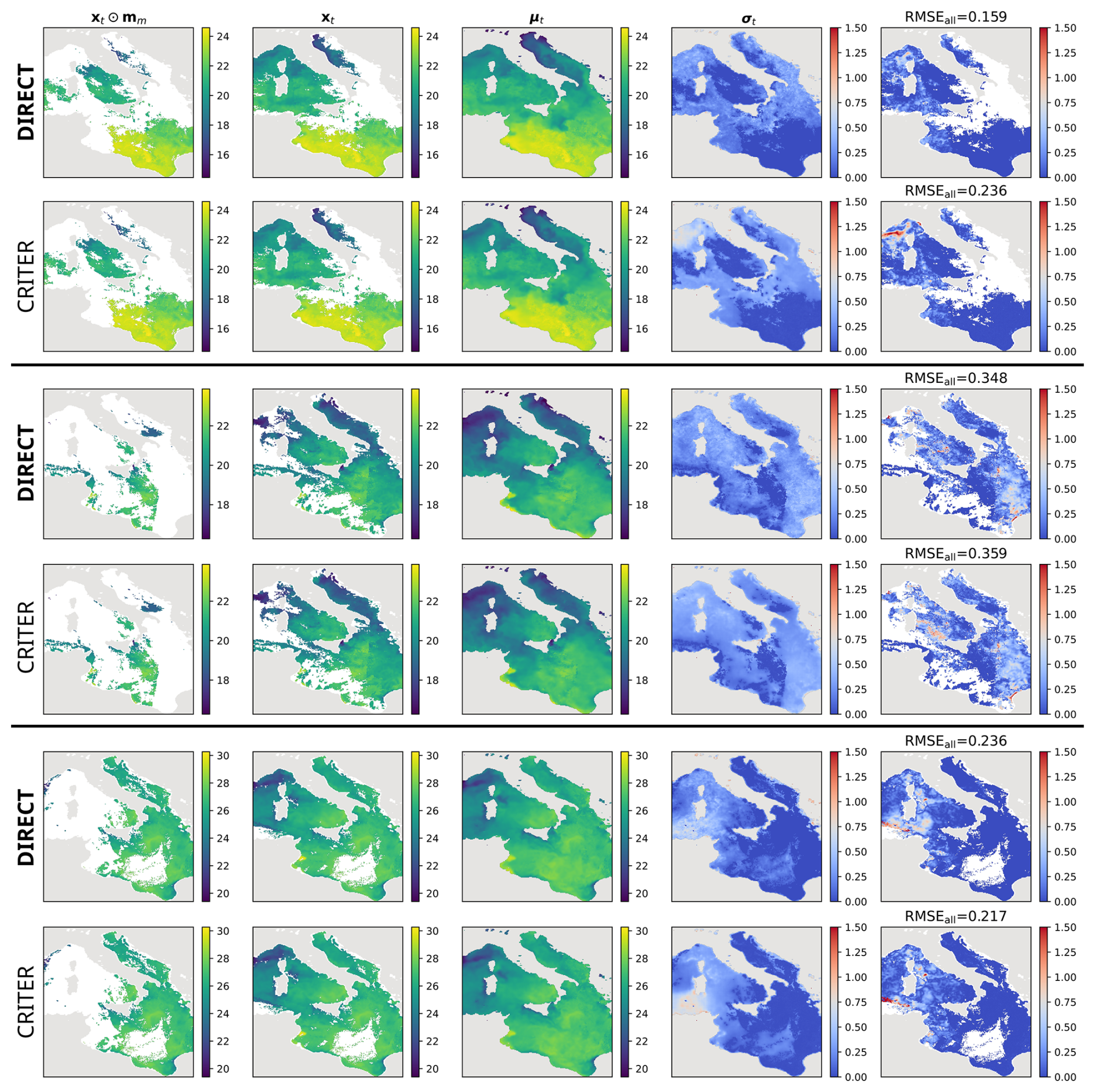
Figure 6 Comparison of DIRECT and CRITER reconstructions on the Mediterranean region. The columns show (from left to right): the partially observed input (x_t⊙m_m), the ground truth x_t, the reconstruction μ_t, the estimated uncertainty σ_t, and the absolute reconstruction error (RMSE_all). All values are in °C.

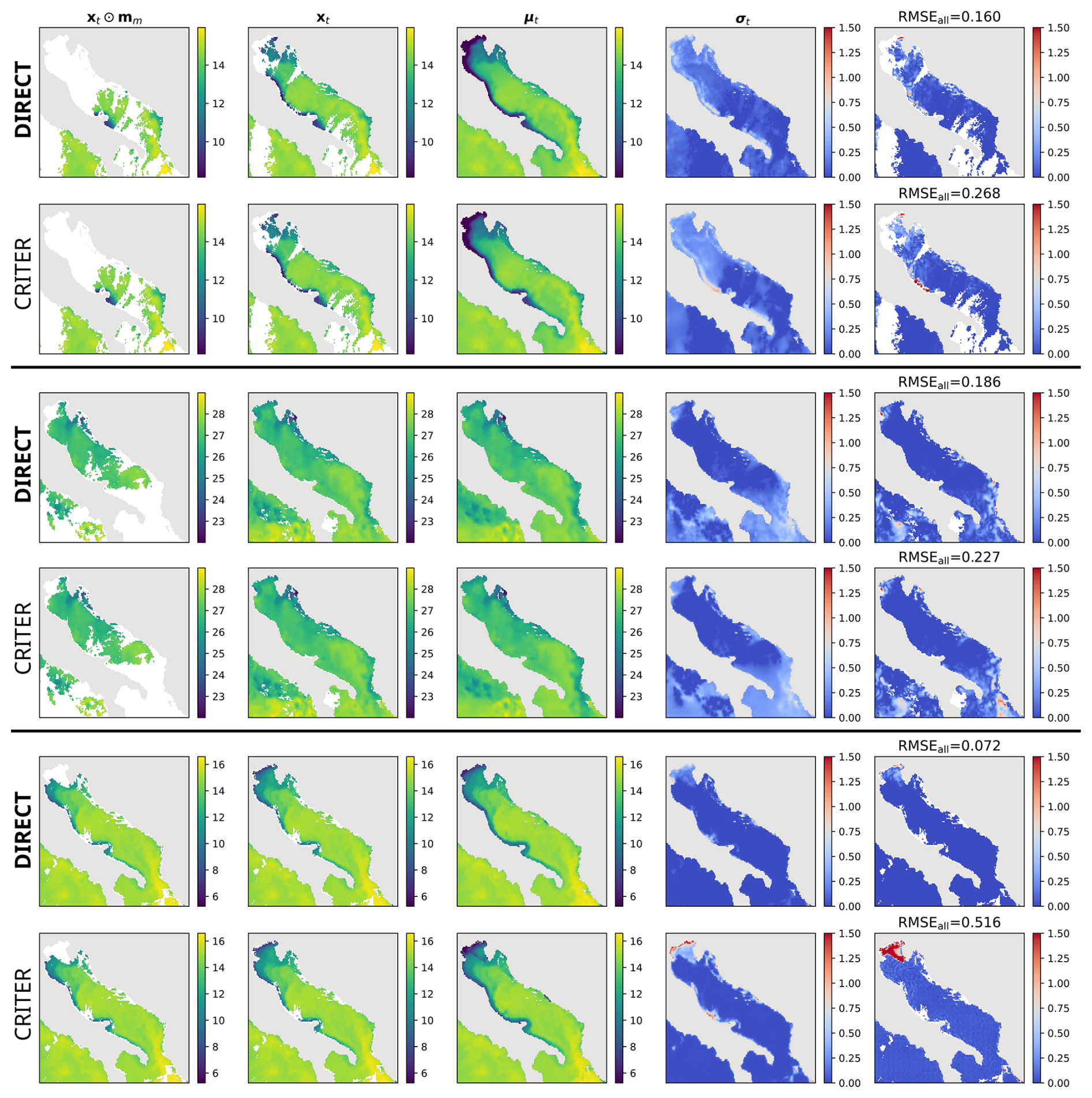
Figure 7 Comparison of DIRECT and CRITER reconstructions on the Adriatic region. The columns show (from left to right): the partially observed input (x_t⊙m_m), the ground truth x_t, the reconstruction μ_t, the estimated uncertainty σ_t, and the absolute reconstruction error (RMSE_all). All values are in °C.

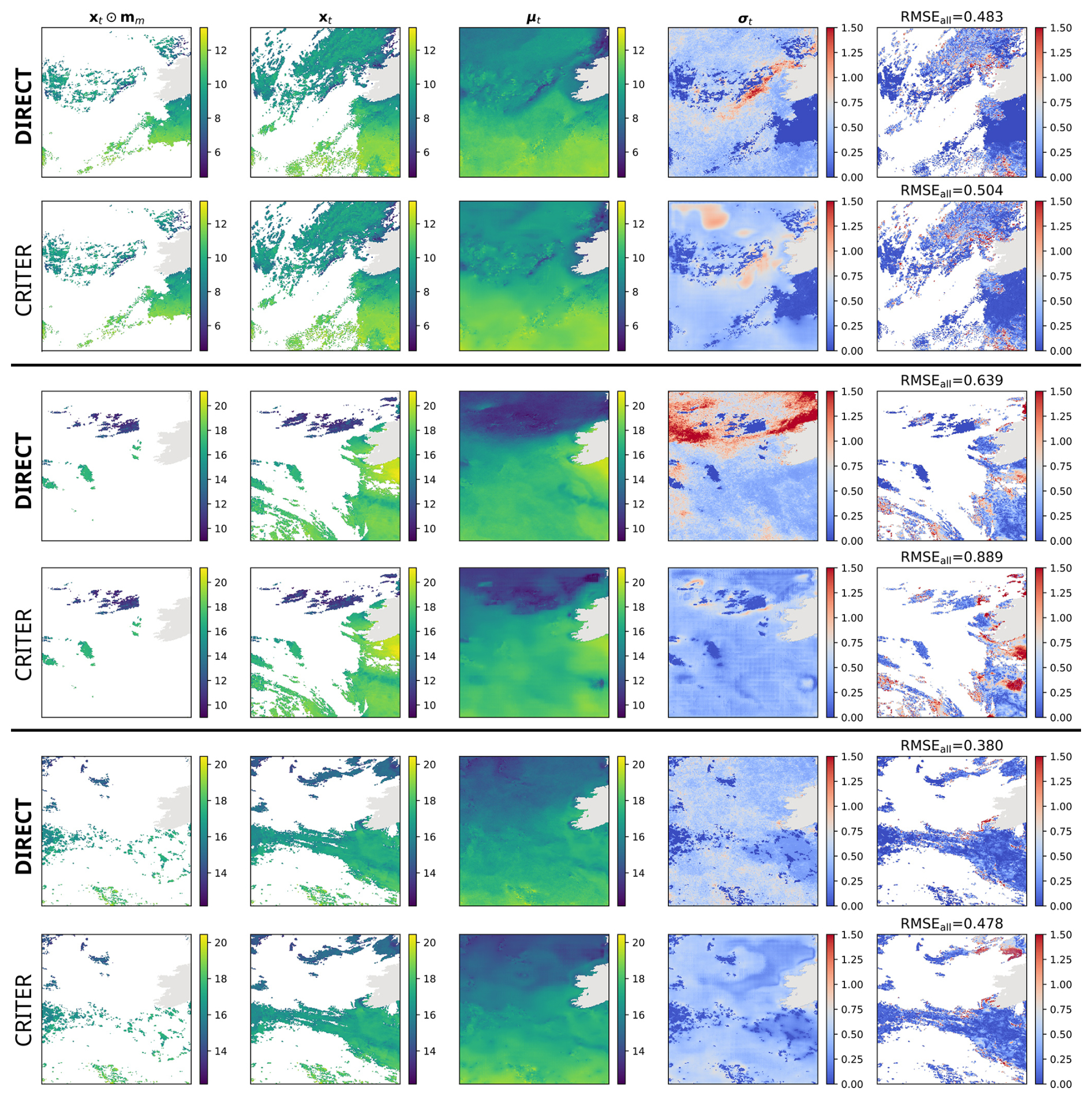
Figure 8 Comparison of DIRECT and CRITER reconstructions on the Atlantic region. The columns show (from left to right): the partially observed input (x_t⊙m_m), the ground truth x_t, the reconstruction μ_t, the estimated uncertainty σ_t, and the absolute reconstruction error (RMSE_all). All values are in °C.

4.2.1 Comparison with operational L4 products

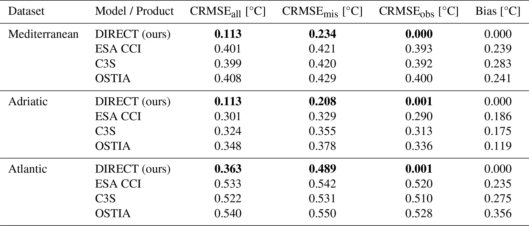
We compare DIRECT against operational gap-free Level-4 (L4) SST products, based on variational data assimilation and optimal interpolation, distributed by the Copernicus Marine Service: the reprocessed OSTIA analysis (E.U. Copernicus Marine Service Information (CMEMS), 2026b), the ESA SST CCI and C3S reprocessed analyses (E.U. Copernicus Marine Service Information (CMEMS), 2026a). Each product was co-located with SST from our three domain datasets and evaluated as a candidate reconstruction against the same L3 reference used throughout. This comparison should be read as a measure of agreement with our L3 reference, not of reconstruction accuracy. The L4 products also ingest in situ data and data from the same sensors as our L3 source, meaning the pixels we synthetically withhold were in general available to the L4 products. Their error over these pixels is therefore not an out-of-sample gap-filling error as it is for DIRECT. The L4 products additionally carry a systematic offset relative to our L3 reference (Table 2, bias column); to prevent this offset from dominating the comparison, we estimate a per-day mean bias over the observed region, subtract it from each L4 field, and report the resulting centered RMSE (CRMSE).

Table 2 shows that, even after this bias removal, DIRECT remains closer to the L3 reference than any of the operational products in all three regions. Relative to the best-performing L4 product in each region, CRMSE_mis is lower by 44 % on the Mediterranean, 37 % on the Adriatic, and 8 % on the Atlantic, indicating that the remaining gap reflects a difference in spatial structure rather than a mean offset. Note that this does not imply that DIRECT is correspondingly more accurate than objective analysis as a technique; it reflects that DIRECT is trained to reconstruct this specific high-resolution L3 product, whereas the L4 analyses target foundation SST and cross-sensor, temporally consistent fields rather than fidelity to any one regional L3 source. A fair skill comparison would evaluate both against independent in-situ observations such as Argo profiles, which neither assimilates, a direction we leave to future work.

Table 2 Comparison of DIRECT against operational gap-free L4 products, evaluated against the same L3 reference. Note that CRMSE_mis is an error against withheld, independent data only for DIRECT; the L4 analyses ingest the same sensors as our L3 reference, so these pixels were in general available to them. Bias is calculated over the observed region. Errors in °C. Bold indicates the lowest error per column within each dataset.

4.2.2 Comparison under varying cloud coverage

To assess the robustness of DIRECT to varying levels of missing data, we evaluate reconstruction performance across three cloud-coverage regimes, defined by the fraction of missing pixels in the central observation x_t relative to all sea pixels. We define low coverage in the interval [0 %, 60 %], moderate coverage in the interval (60 %, 75 %], and high coverage in the interval (75 %, 100 %]. The test sets span a wide range of coverage: 8.3 %–99 % for the Mediterranean, 3.3 %–95 % for the Adriatic, and 39 %–99 % for the Atlantic.

Figure 9 shows the reconstruction errors (RMSE_all, RMSE_mis, RMSE_obs) for DIRECT and CRITER across the three regimes, where, as before, RMSE_obs is reported for completeness, but provides little insight due to the injection of ground truth values at observed locations. Across all cloud-coverage levels and for all three regions, DIRECT consistently outperforms CRITER. On the Mediterranean, RMSE_mis is reduced by 8 %, 6 %, and 10 % in the low-, medium-, and high-coverage regimes, respectively. Improvements are even greater on the Adriatic, with reductions of 16 %, 12 %, and 9 %. On the Atlantic, where occlusions are more extreme and the problem is inherently more challenging, smaller yet meaningful improvements of 2 %, 4 %, and 6 % are achieved.

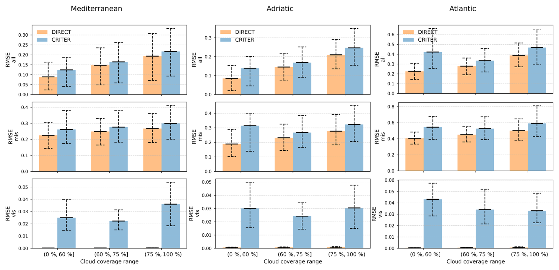
Figure 9 Reconstruction error comparison of DIRECT and CRITER under varying levels of cloud coverage (low, moderate, and high) on the Mediterranean, Adriatic, and Atlantic datasets. The error bars indicate the 10 % percentile, mean, and the 90 % percentile of the error.

4.2.3 Uncertainty estimation and bias analysis

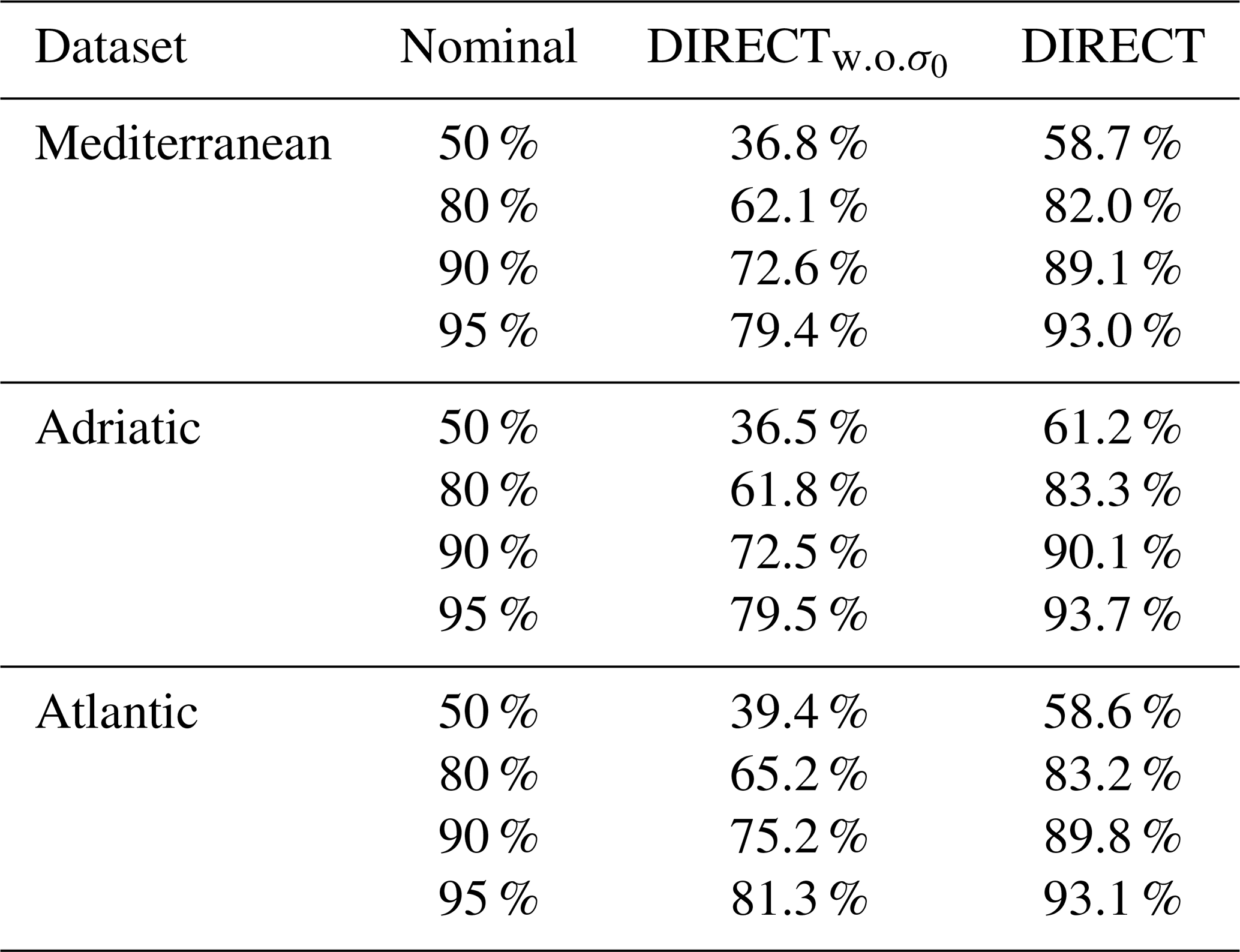
We evaluate the reliability of ensemble-based uncertainty estimates over the withheld regions using two complementary measures: the scaled error ϵ of Eq. (5) and the empirical coverage of the nominal 50 %, 80 %, 90 %, and 95 % central prediction intervals, where a withheld pixel is covered at level p when ∣ϵ∣≤z_p for the standard-normal quantile z_p. Results for the raw ensemble and after correction are given in Tables 3 and 4. Without the correction (${\text{DIRECT}}_{\mathrm{w}.\mathrm{o}.{\mathit{\sigma }}_{\mathrm{0}}}$), the ensemble is under-dispersed, with σ_ϵ>1.7 and coverage below nominal at every level and in all three regions. The two measures together indicate two distinct effects. Coverage is depressed across the full range of levels, including the central 50 % interval, which reflects a broad under-dispersion of the ensemble. At the same time, the large σ_ϵ points to pronounced ensemble collapse at a sparse set of pixels, where the samples become nearly identical and the predicted variance is far too small. The learned regularization constant σ₀ (0.135 for Mediterranean, 0.101 for Adriatic, 0.298 for Atlantic), added in Eq. (3), addresses both effects. It raises the overall spread, correcting the global under-dispersion, and places a floor on the variance at collapsed pixels. With the correction, σ_ϵ falls close to one and coverage approaches nominal at the 80 %, 90 %, and 95 % levels across all datasets. As a single global offset applied uniformly across pixels and probability levels, σ₀ does not achieve exact calibration everywhere: the corrected 50 % intervals slightly over-cover (about 59 %–61 %) and the 95 % intervals slightly under-cover (about 93 %–94 %), since one constant cannot adapt to spatially varying error regimes or to the tails of the distribution. Overall, σ₀ accounts for 34 %, 25 %, and 36 % of the total variance across the Mediterranean, Adriatic, and Atlantic datasets, respectively.

Table 3 Uncertainty estimation analysis of DINCAE2, CRITER, and DIRECT. Mean standardized error (μ_ϵ), standard deviation (σ_ϵ), and bias are reported for each dataset. Bold indicates the value closest to the ideal in each column within a dataset (μ_ϵ→0, σ_ϵ→1, bias →0).

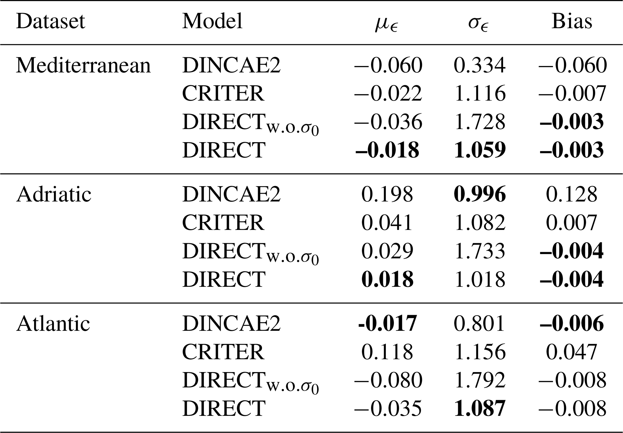
Table 4 Empirical coverage of nominal central prediction intervals, before (${\text{DIRECT}}_{\mathrm{w}.\mathrm{o}.{\mathit{\sigma }}_{\mathrm{0}}}$) and after (DIRECT) the σ₀ correction.

4.2.4 Power spectrum density analysis

To evaluate how well DIRECT preserves spatial variability across scales, we perform a power spectral density (PSD) analysis (Stoica et al., 2005) on a region of interest (ROI) in the central Mediterranean and compare it with CRITER (Zupančič Muc et al., 2025). Time frames for which the ROI is fully observed are first identified, after which cloud masks are sampled, obscuring between 51 % and 100 % of the ROI. Both models reconstruct the full SST field from these masked inputs. For each reconstruction, we first remove the large-scale spatial background by subtracting a least-squares linear plane fitted over the ROI, which suppresses the anisotropic low-wavenumber trend. We then compute the 2D gradient magnitude $\left|\right|\mathrm{\nabla }{\mathit{\mu }}_t^{\text{ROI}}|{|}_{\mathrm{2}}$ and the isotropic PSD using a FFT with a Blackman–Harris window (Harris, 1978).

Figures 10d and 11d show that both models reproduce the large-scale spectral structure of the SST field and follow the ground-truth spectrum closely from the largest scales down to intermediate wavenumbers. At higher wavenumbers both models depart from the ground truth and settle at similar energy levels. For CRITER, however, this small-scale energy is largely non-physical: the gradient-magnitude fields (Figs. 10c and 11c) reveal grid-like block artifacts, a byproduct of patch-based processing. In contrast, DIRECT's energy profile reflects coherent, albeit slightly smoothed, oceanic structures. The same gradient-magnitude fields show no discontinuity tracing the boundary between observed and reconstructed regions (Fig. 11c), indicating that the FUSE re-injection does not introduce a visible seam despite anchoring the output to measured pixels at every step. DIRECT therefore provides a more physically faithful representation of the continuum, avoiding both the spurious grid-like artefacts that inflate the PSD of patch-based baselines and the boundary artifacts that might be expected from observation re-injection.

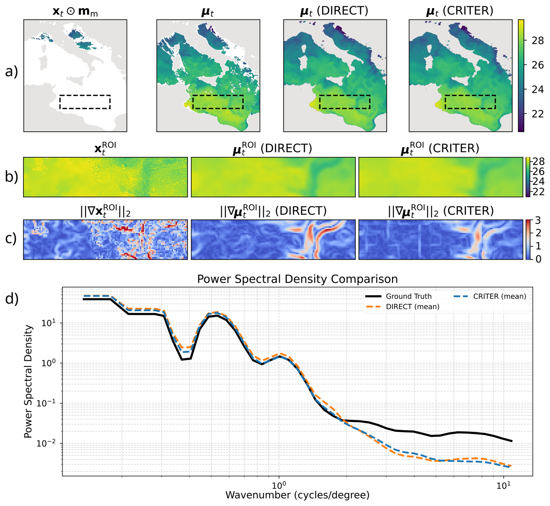
Figure 10 Power spectral density (PSD) analysis for a selected region of interest (ROI). (a) Masked SST input, ground truth field, and reconstructions from DIRECT and CRITER. (b) Zoomed views of the ROI. (c) Gradient magnitudes $\left|\right|\mathrm{\nabla }{\mathit{\mu }}_t^{\text{ROI}}|{|}_{\mathrm{2}}$ highlighting structural differences. (d) Isotropic PSD computed from the plane-detrended ROI fields using an FFT with a Blackman–Harris window. The displayed curves represent the average spectral density across 10 independent mask realizations.

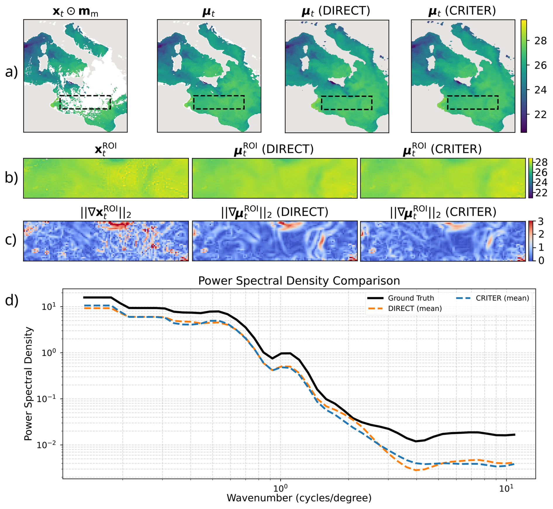
Figure 11 Power spectral density (PSD) analysis for a selected region of interest (ROI). (a) Masked SST input, ground truth field, and reconstructions from DIRECT and CRITER. (b) Zoomed views of the ROI. (c) Gradient magnitudes $\left|\right|\mathrm{\nabla }{\mathit{\mu }}_t^{\text{ROI}}|{|}_{\mathrm{2}}$ highlighting structural differences. (d) Isotropic PSD computed from the plane-detrended ROI fields using an FFT with a Blackman–Harris window. The displayed curves represent the average spectral density across 10 independent mask realizations.

4.2.5 Analysis of spatial scale correlation

To assess the preservation of spatial structure and mesoscale variability beyond pixel-wise error, we analyze the spatial correlation properties using empirical semivariograms (Matheron, 1963). Semivariance is computed as

$$\begin{array}{}\text{(7)}& \mathit{\gamma }\left(d\right)={\displaystyle \frac{\mathrm{1}}{\mathrm{2}N\left(d\right)}}\sum _{i,j\in \mathcal{P}\left(d\right)}(p_i-p_j{)}^{\mathrm{2}},\end{array}$$

where 𝒫(d) denotes the set of N(d) pixel pairs separated by distance d, and p_i is the observation value of x_t at ith pixel. For statistical robustness, the analysis is averaged over 10 independent mask realizations sampled from the Mediterranean dataset.

As shown in Figs. 12 and 13, both models effectively capture local correlations (short lags). At intermediate to larger spatial lags, however, clearer differences appear. In the hidden region variograms, DIRECT consistently reproduces the growth of semivariance with distance more faithfully, while CRITER exhibits less stable long-range behavior, suggesting a struggle to maintain spatial coherence over large obscured gaps. When considering the full valid SST domain, the performance gap narrows significantly. In this setting, both DIRECT and CRITER follow the ground truth semivariance almost perfectly, with virtually no observable difference between the two models. This convergence is expected, as the calculation includes observed pixels. The results highlight that while both models are highly reliable when observations are present, DIRECT provides a more physically consistent spatial texture when reconstructing larger completely unobserved areas.

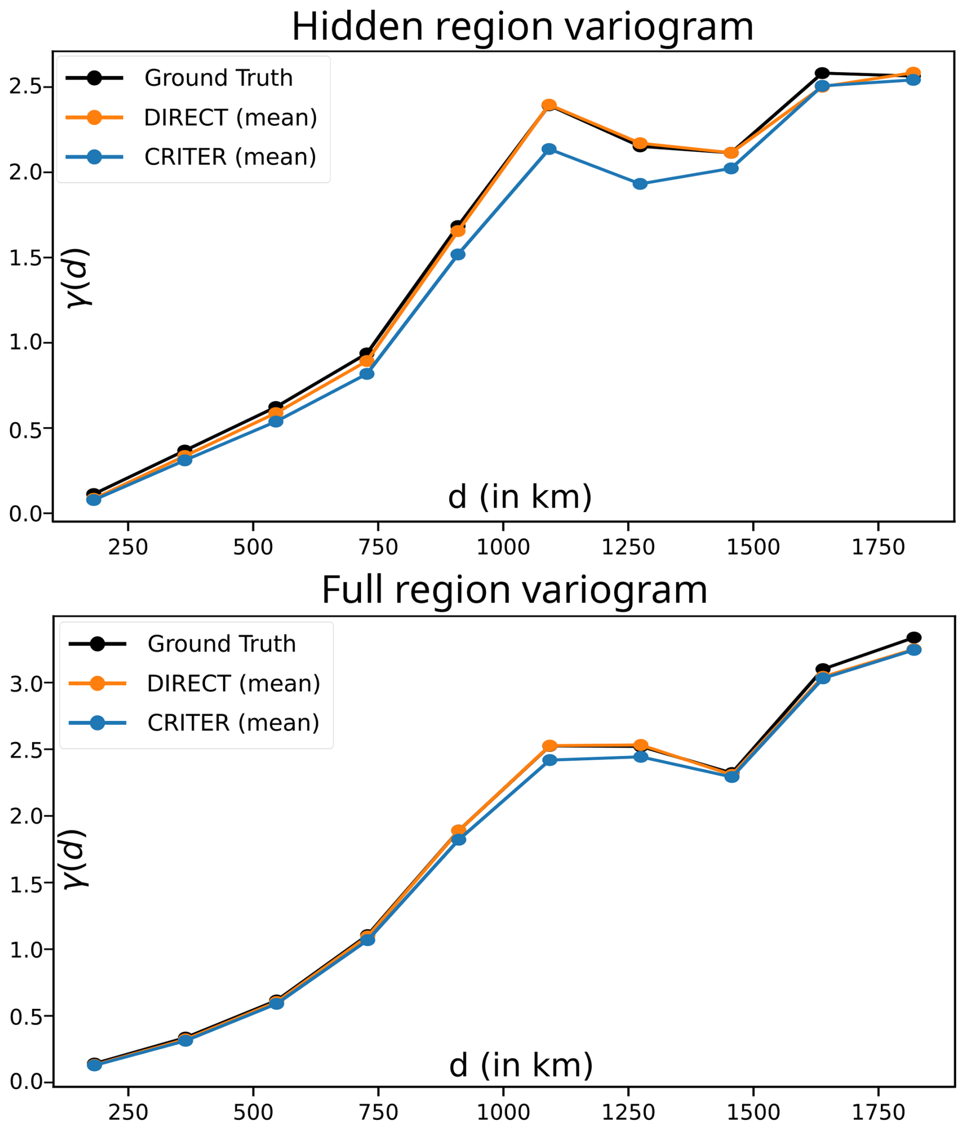
Figure 12 Visualization of the spatial scales and correlation properties analysis. Top plot: empirical semivariograms computed exclusively over hidden regions. Bottom plot: semivariograms computed over the full SST domain. Each curve represents the mean semivariance across 10 different mask realizations.

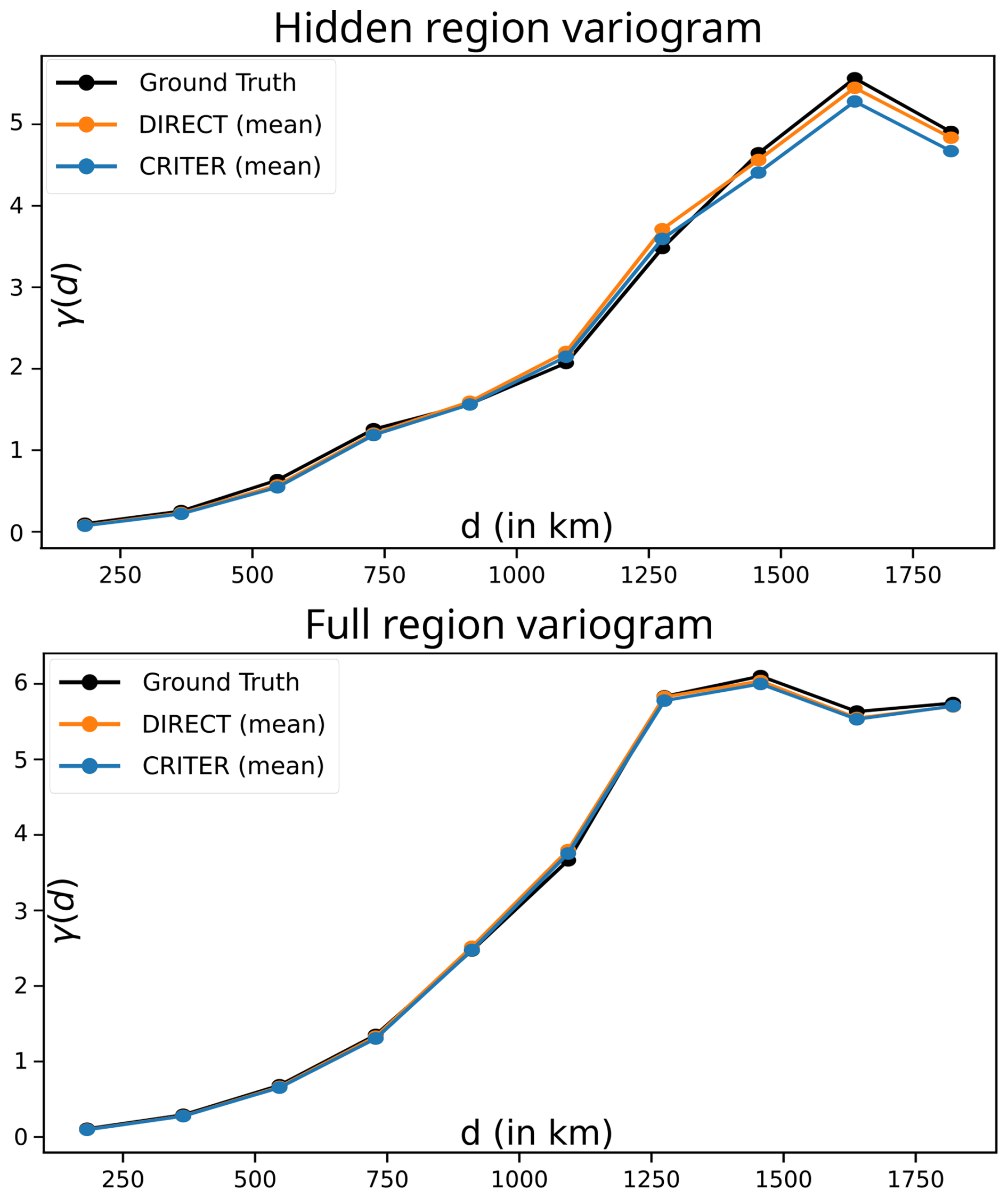
Figure 13 Visualization of the spatial scales and correlation properties analysis. Top plot: empirical semivariograms computed exclusively over hidden regions. Bottom plot: semivariograms computed over the full SST domain. Each curve represents the mean semivariance across 10 different mask realizations.

4.2.6 Continuous Ranked Probability Score (CRPS)

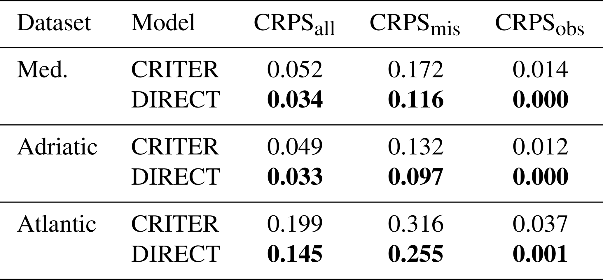
The Continuous Ranked Probability Score (CRPS) (Matheson and Winkler, 1976) was evaluated over all three regions, and results are shown in Table 5. This provides a measure for evaluating probabilistic predictions by comparing the entire forecast distribution against the observed value. Unlike traditional deterministic error metrics, which assess only the mean reconstruction, the CRPS quantifies accuracy, statistical reliability, and sharpness of the predictive distribution. Rather than simply assessing whether DIRECT obtains a plausible distribution, the CRPS allows us to qualify if the produced ensemble actually explores the inherent uncertainty in the reconstruction and if probabilities derived from the ensemble are reliable. For DIRECT, the CRPS is computed empirically from the reconstruction ensemble. As CRITER does not produce an ensemble but instead predicts a per-pixel mean and variance, we compute its CRPS by drawing samples from the corresponding per-pixel Gaussian. Across all three regions, DIRECT achieves lower CRPS than CRITER, indicating that its ensemble provides a sharper and better-calibrated predictive distribution. As with the pointwise reconstruction errors, CRPS over the missing pixels is highest in the Atlantic region, reflecting the more extensive cloud cover and more energetic ocean variability.

Table 5 Continuous Ranked Probability Score of CRITER and DIRECT over the whole region, the missing region, and the observed region. The values are in °C. Med. denotes the Mediterranean dataset. Bold indicates the best result per column within each dataset.

4.3 Ablation study

Ablation studies were performed on the Mediterranean dataset, unless stated otherwise, to expose the influences of individual parts.

4.3.1 Importance of input rectification (FUSE)

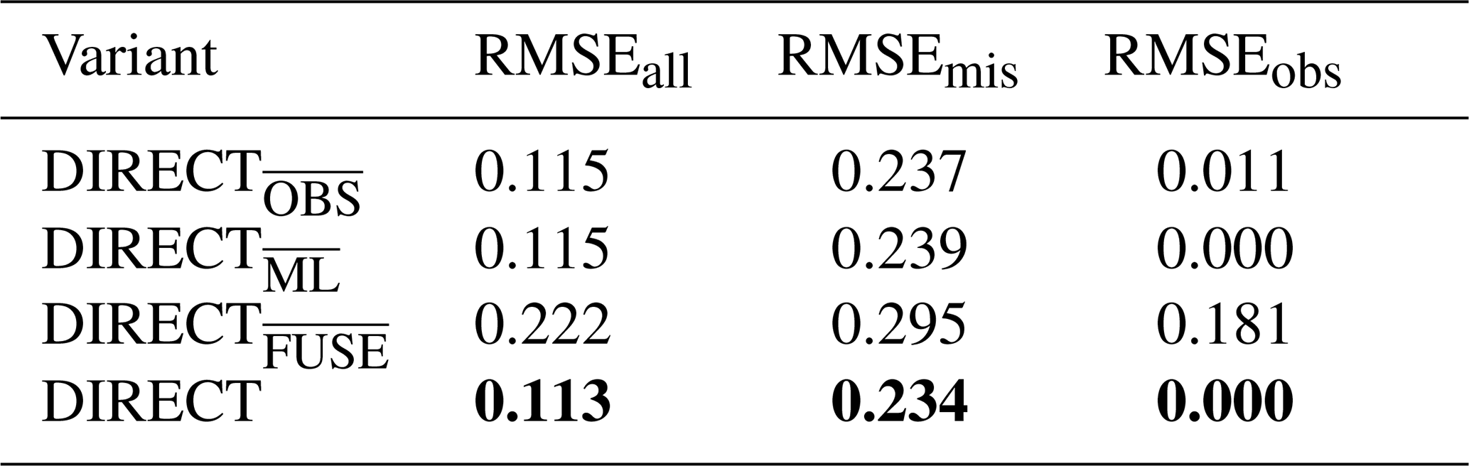
We study the effect of the FUSE procedure (Eq. 2) by comparing DIRECT with three ablated variants: one without injecting observed SST values (${\text{DIRECT}}_{\stackrel{\mathrm{‾}}{\text{OBS}}}$), one without zeroing land pixels (${\text{DIRECT}}_{\stackrel{\mathrm{‾}}{\text{ML}}}$), and one without any rectification (${\text{DIRECT}}_{\stackrel{\mathrm{‾}}{\text{FUSE}}}$). Results in Table 6 show that completely disabling FUSE causes a large drop in reconstruction accuracy, with RMSE_mis increased by more than 20 %. Restoring only the injection of SST values (${\text{DIRECT}}_{\stackrel{\mathrm{‾}}{\text{ML}}}$) or only the masking of land pixels (${\text{DIRECT}}_{\stackrel{\mathrm{‾}}{\text{OBS}}}$) recovers much of this loss (only a 2 % increase for both), indicating that both corrections help anchor the generative process and prevent errors from accumulating across integration steps. The best results are obtained when both corrections are applied, confirming that the full FUSE procedure provides complementary benefits and stabilizes the flow integration process.

Table 6 Performance of DIRECT variants. All of the reported reconstruction errors are in °C. Bold indicates the best result per column within each dataset.

4.3.2 Importance of seasonal context

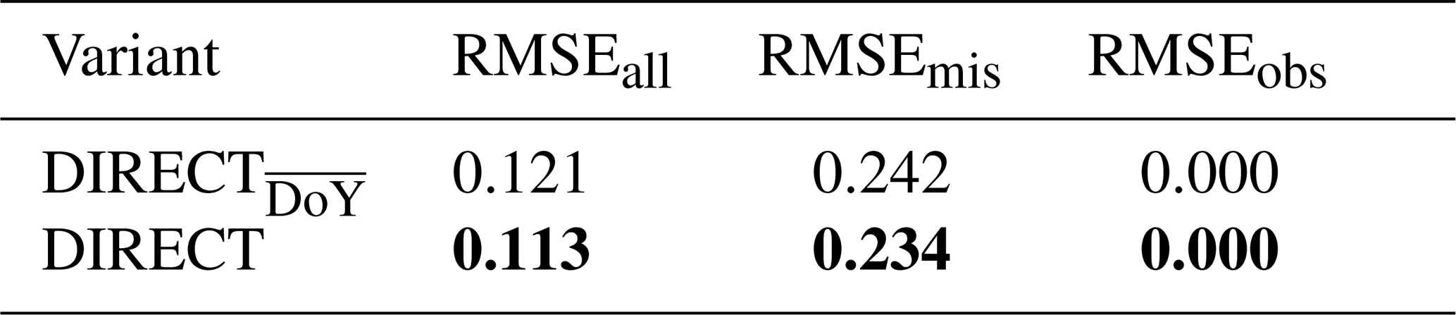
Similarly to DINCAE2 (Barth et al., 2022) and CRITER (Zupančič Muc et al., 2025), DIRECT incorporates seasonal context through the sine and cosine of the day-of-year d_t, which encode the annual cycle. To evaluate the contribution of this information, we trained a variant ${\text{DIRECT}}_{\stackrel{\mathrm{‾}}{\text{DoY}}}$ that excludes DoY embeddings. As shown in Table 7, removing seasonal context increases RMSE_mis from 0.234 to 0.242, corresponding to a relative degradation of about 3 %. Although the effect is modest, this indicates that DoY features provide useful information.

Table 7 Performance of DIRECT and ${\text{DIRECT}}_{\stackrel{\mathrm{‾}}{\text{DoY}}}$, which is without the day-of-year information. All of the reported reconstruction errors are in °C. Bold indicates the best result per column within each dataset.

4.3.3 Influence of mask-aware conditioning

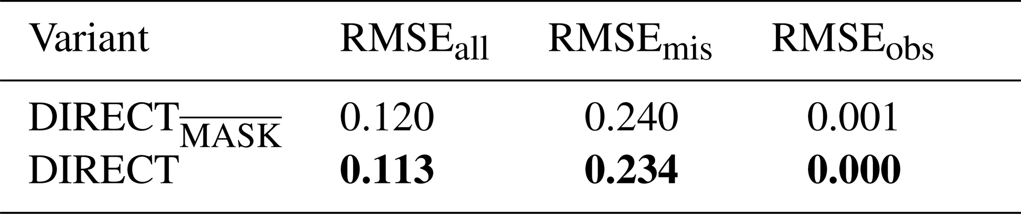
DIRECT incorporates one-hot encoded masks that distinguish between observed pixels, filled pixels originating from temporally shifted frames, and missing or land pixels. To evaluate the importance of these masks, we trained a variant ${\text{DIRECT}}_{\stackrel{\mathrm{‾}}{\text{MASK}}}$ that excludes all mask information. As shown in Table 8, removing mask-aware conditioning increases RMSE_mis from 0.234 to 0.240, a relative degradation of about 3 %. Although the effect is modest, the masks provide a consistent benefit by guiding the model to focus on reliable inputs.

Table 8 Performance of DIRECT and ${\text{DIRECT}}_{\stackrel{\mathrm{‾}}{\text{MASK}}}$, which does not utilize one hot encoded masks. All of the reported reconstruction errors are in °C. Bold indicates the best result per column within each dataset.

4.3.4 One-hot encoding vs. offset masks

In the default DIRECT formulation, temporal origins of filled pixels are encoded using one-hot masks with three channels per auxiliary frame. As an alternative, we evaluate DIRECT_OFFSETS, which replaces the one-hot representation with a single binary mask and an integer offset map that encodes the temporal origin directly: −1, −2, and −3 indicate pixels sourced from t−1, t−2, and t−3, respectively, while a value of 0 marks missing or invalid pixels. The offset map for the future frame (t+1) is constructed in the same way, with values +1, +2, and +3. Table 9 confirms that both approaches perform similarly, with the one-hot representation giving a slight edge (less than 1 %). This suggests that compressed offset maps are a viable alternative when reducing input channels is desirable.

Table 9 Performance of DIRECT and DIRECT_OFFSETS. All of the reported reconstruction errors are in °C. Bold indicates the best result per column within each dataset.

4.3.5 Influence of reconstruction ensemble size

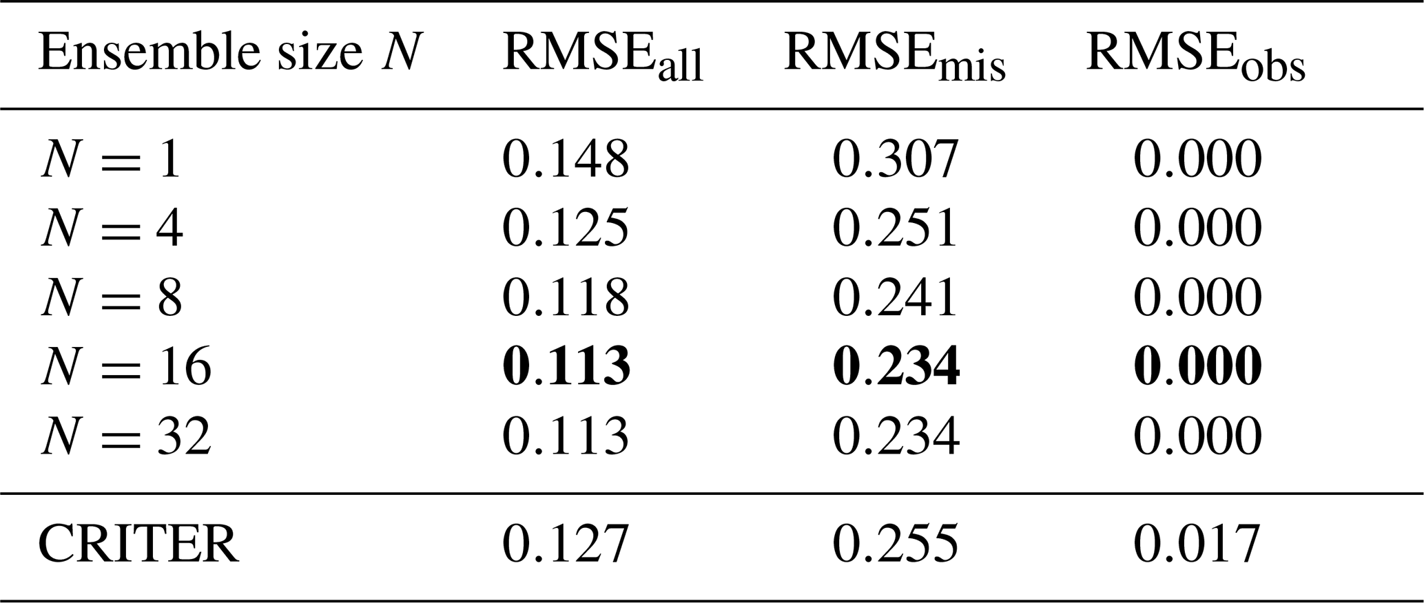
Because DIRECT is a generative model, multiple reconstructions can be sampled for a single input by varying the initial noise seed. As per Sect. 2.2, these samples are averaged to produce the final reconstruction. Table 10 shows that averaging just N=4 reconstructions already reduces RMSE_mis by 18 % compared to N=1, and crucially, this already outperforms the deterministic state-of-the-art CRITER. Our default N=16 yields a 23 % improvement compared to N=1. Although larger ensembles (e.g. N=32) are comparable with our default, they also increase inference time, making 16 samples practical and effective.

Figure 14 illustrates the ensemble characteristics. The mean field provides a stable and accurate reconstruction, while the per-pixel standard deviation captures uncertainty in obscured regions. The residuals ${\mathbf{\Delta }}_n={\mathit{\mu }}_t-{\widehat{\mathit{x}}}_{t,n}$ (Rows 2–4) highlight the diverse high-frequency fluctuations present in individual samples.

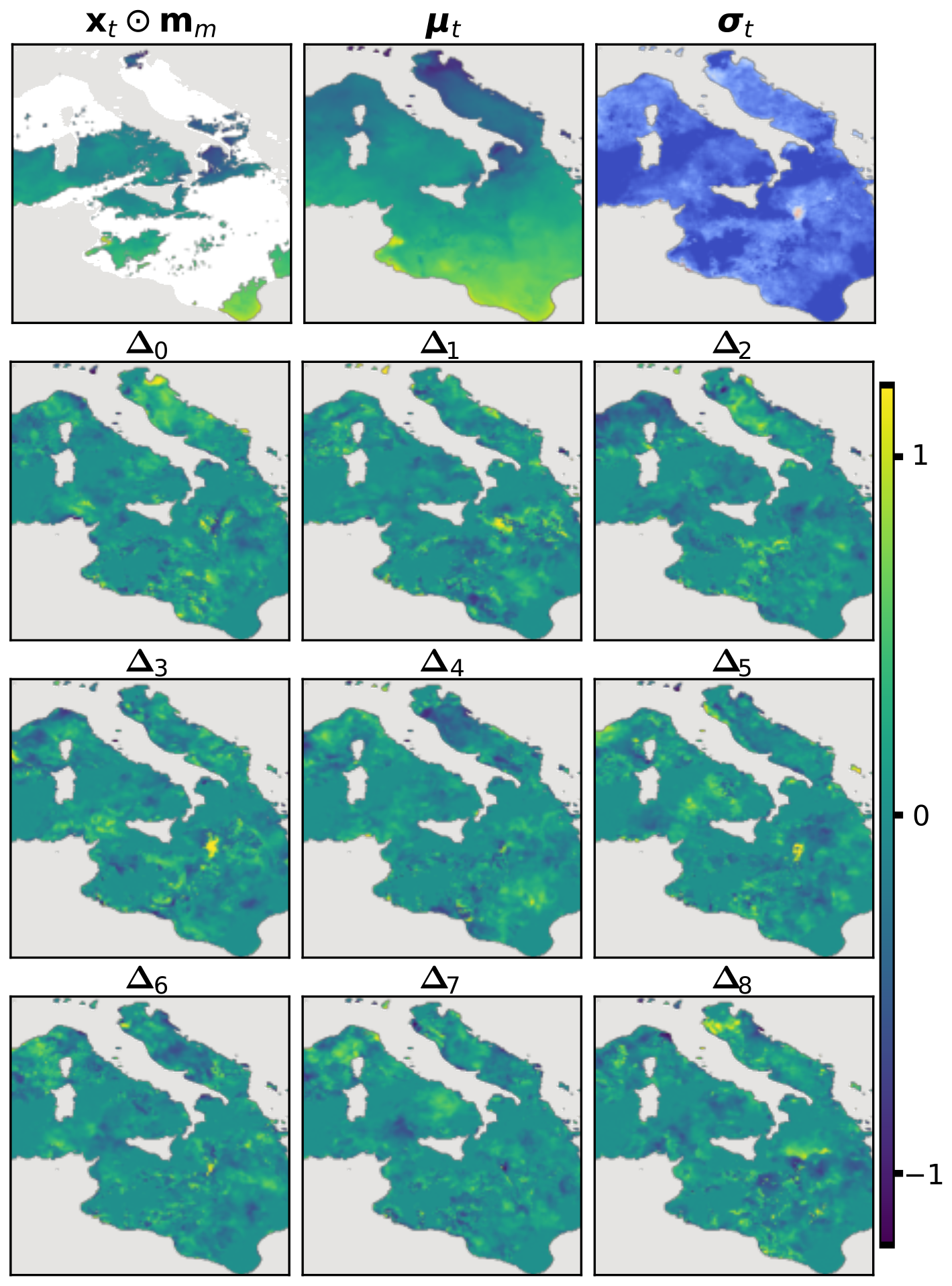
Figure 14 A visualization of a reconstruction ensemble. The first row shows the masked input, the ensemble mean (μ_t) and the per-pixel uncertainty (σ_t). Rows 2–4 visualize the residual fields ${\mathit{\mu }}_t-{\widehat{\mathit{x}}}_{t,n}$ for nine independent samples, illustrating the high-frequency structural diversity.

Table 10 Performance impact of ensemble size N on reconstruction accuracy. All of the reported reconstruction errors are in °C. Bold indicates the default configuration used throughout the paper.

4.3.6 Influence of multi-pass reconstruction

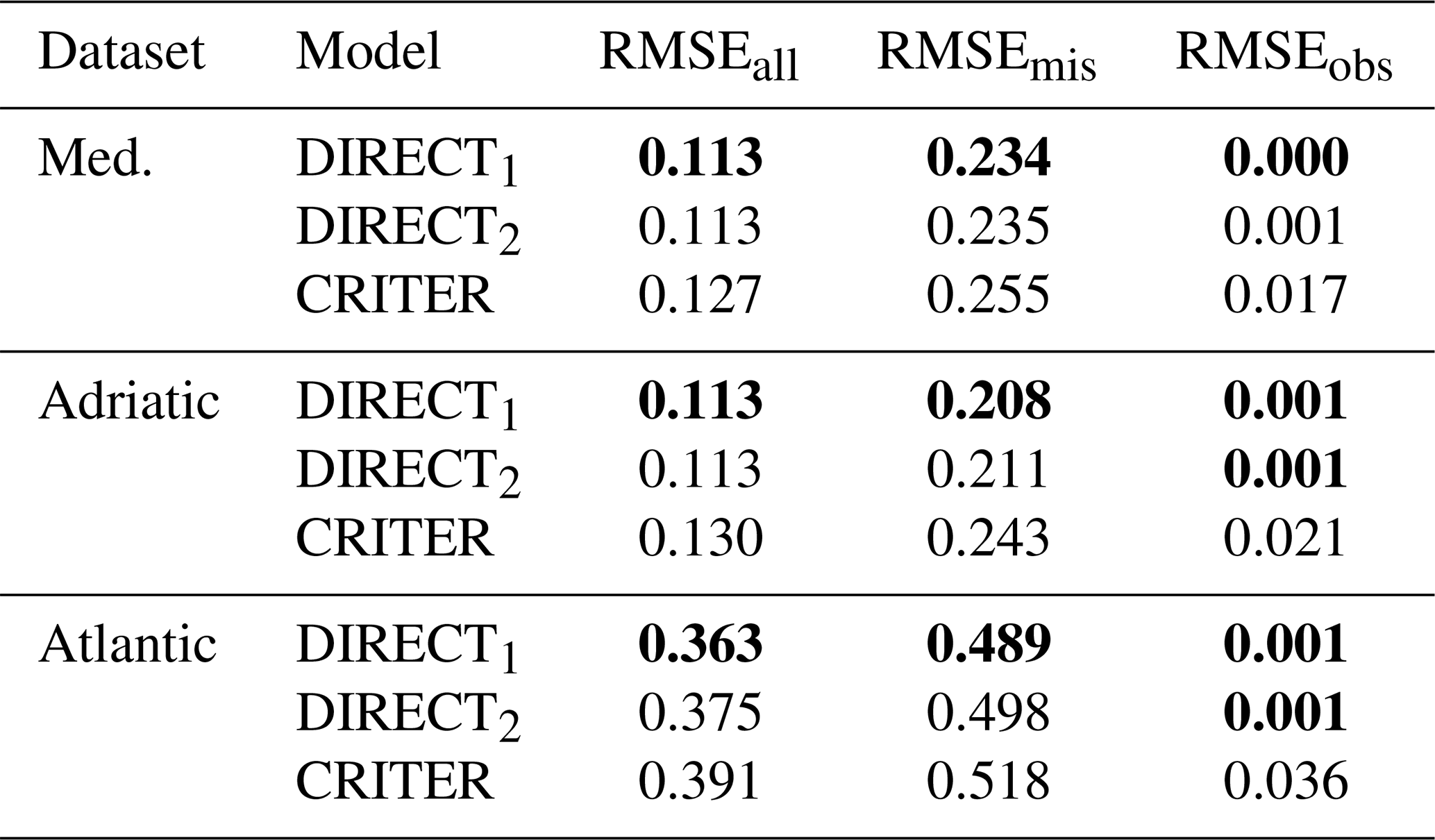
We evaluated a multi-pass inference strategy to test whether iteratively refining the temporal context improves the final reconstruction. In the default single-pass formulation (DIRECT₁), missing measurements in the temporal context (days t−1 and t+1) are opportunistically filled using the closest available observations. In the multi-pass formulation (${\text{DIRECT}}_{N_p}$), we attempt to improve the central day's estimate by running the reconstruction of the entire time-series in multiple passes, substituting the missing values in the context days with the model's own predictions from the previous pass.

However, as summarized in Table 11, the two-pass strategy (DIRECT₂) yields performance comparable to, or slightly worse than, the single-pass baseline (DIRECT₁) across all datasets. In the Mediterranean and Adriatic regions, the reconstruction error in missing regions (RMSE_mis) increases slightly from 0.234 to 0.235 and from 0.208 to 0.211, respectively. On the Atlantic dataset – which is characterized by persistent, large-scale cloud cover – the error increases from 0.489 to 0.498.

These results indicate that substituting the initial fallback context with the model's own first-pass estimates propagates reconstruction uncertainties and errors rather than providing a cleaner conditioning signal.

Table 11 Influence of the multi-pass strategy (DIRECT₂), compared to the single-pass (DIRECT₁) and CRITER. All reported reconstruction errors are in °C. Med. denotes the Mediterranean dataset. Bold indicates the best result per column within each dataset.

4.3.7 Influence of future temporal context

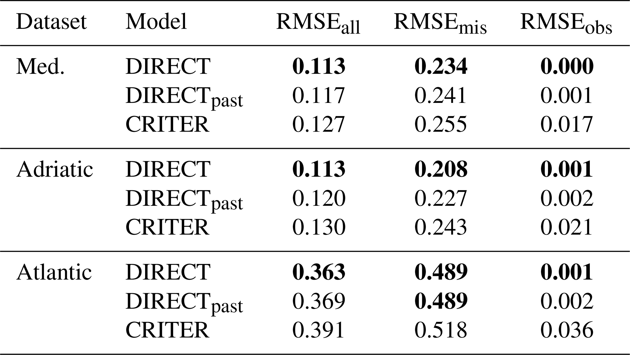
In our default formulation, DIRECT utilizes a temporal context spanning both past and future observations (t−1 and t+1) to reconstruct the central day t. This bidirectional approach is standard for historical gap-filling tasks, as it allows the model to smoothly interpolate the evolution of ocean dynamics. However, for Near Real-Time (NRT) operational settings, future observations are strictly unavailable. To evaluate DIRECT's viability in such scenarios, we trained a past-only variant (DIRECT_past) that conditions the network solely on the preceding frame (t−1) and the central frame (t).

Table 12 compares DIRECT_past against the default DIRECT. As expected, removing the future context leads to a slight degradation in performance compared to the default model. In the Mediterranean and Adriatic regions, the reconstruction error in missing regions (RMSE_mis) increases from 0.234 to 0.241, and from 0.208 to 0.227, respectively. On the Atlantic dataset, performance remains unchanged. This confirms that future information naturally aids the model in accurately resolving the temporal evolution of highly dynamic ocean events.

Crucially, despite lacking future temporal anchoring, DIRECT_past still consistently outperforms the state-of-the-art CRITER across all three regions. This demonstrates that DIRECT's generative prior and observation-guided rectification remain highly effective even under strict constraints, making the architecture highly suitable for daily operational NRT applications.

Table 12 Influence of future temporal context. The past-only variant (DIRECT_past) is compared to the default model (DIRECT) and the CRITER baseline. All reported reconstruction errors are in ^∘C. Med. denotes the Mediterranean dataset. Bold indicates the best result per column within each dataset.

4.3.8 Incorporating microwave observations

DIRECT operates on high-resolution infrared L3 observations, which are unavailable under cloud cover. Microwave radiometers, however, do retrieve SST through clouds, albeit at substantially coarser spatial resolution, and therefore offer a potential source of information beneath clouds. Because DIRECT ingests its spatio-temporal context through a lightweight input projection, additional observation sources can be added with minimal architectural change. To demonstrate this, we conducted a preliminary experiment on the Mediterranean dataset using the daily microwave optimally-interpolated SST product MW OI SST v5.1 (Remote Sensing Systems, 2022), regridded and co-located to our domain. The microwave field is supplied as an additional input by embedding it through a separate convolution branch and summing it with the projected context, mirroring the treatment of C_2t (denoted DIRECT_MW).

As shown in Table 13, the microwave variant leaves reconstruction accuracy essentially unchanged, with RMSE_mis marginally lower than the default model. We attribute the small effect to the coarse resolution of the microwave product relative to the infrared L3 fields. The purpose of the experiment is not to demonstrate an accuracy gain but to show that DIRECT is readily extensible to heterogeneous observation sources. A more careful treatment of the resolution mismatch and observation-specific uncertainty, together with an evaluation in regimes of persistent, large-scale cloud cover where cloud-penetrating observations are expected to be most valuable, is a promising direction that we leave to future work.

Table 13 Effect of incorporating microwave (MW) observations on the Mediterranean dataset. All reported reconstruction errors are in °C. Med. denotes the Mediterranean dataset.

5 Discussion

DIRECT reconstructs an L3 satellite product, which is itself a retrieval carrying sensor noise and residual cloud contamination. Our metrics are computed against this product, thus the reported residuals combine reconstruction error with the observation error already present in the reference. The FUSE step re-injects the measured pixels at every integration step and thus inherits their noise, a deliberate trade-off in exchange for hard observation consistency. The model does not depend critically on this choice: the variant that disables observation re-injection (${\text{DIRECT}}_{\stackrel{\mathrm{‾}}{\text{OBS}}}$, Sect. 4.3.1) still reconstructs the missing regions to state-of-the-art accuracy, showing that performance is driven by the generative prior rather than the re-injection alone. Both training and evaluation use cloud masks from other days, which enables learning without cloud-free ground truth. Two consequences follow. Cloud occurrence is coupled to the atmospheric state and hence to SST variability, thus the missingness is not strictly independent of the field being reconstructed. And because we synthetically withhold observed pixels, the evaluation measures reconstruction skill against a known reference rather than validating under genuine cloud conditions. The temporal context uses a fixed three-day window, following prior evidence that most relevant temporal information lies within a few surrounding days. This is limited when informative observations fall outside the window, most notably during cloud systems that persist over many days. Cloud-penetrating microwave observations are well suited to these conditions, and our preliminary experiment (Sect. 4.3.8) shows that DIRECT incorporates such a source with minimal architectural change, making a more thorough integration targeted at persistent-cloud regimes a natural next step. Finally, two aspects bound reconstruction quality. The ensemble mean is stable and accurate, but averaging acts as a low-pass filter that attenuates part of the fine-scale variability present in individual samples. The uncertainty is calibrated with a single global variance offset, which removes the dominant under-dispersion and brings coverage close to nominal (Sect. 4.2.3) but cannot correct calibration that varies across space or across the tails. Spatially adaptive calibration, and a training-time scoring-rule objective in place of the post-hoc correction, are promising routes to sharper estimates.

6 Conclusions

We presented DIRECT, a diffusion-inspired generative model for reconstructing dense SST fields from partially observed satellite measurements. By formulating SST gap-filling as a conditional flow-matching task, DIRECT departs from deterministic reconstruction and instead produces an ensemble of physically plausible realizations, enabling both accurate reconstructions and spatially resolved uncertainty estimation. The model combines temporal context, seasonal conditioning, and observation-guided rectification within a single end-to-end framework, and is trained directly on sparse observations without cloud-free ground truth. Experimental results across Mediterranean, Adriatic, and Atlantic datasets show that DIRECT consistently outperforms current state-of-the-art methods, reducing reconstruction error in occluded regions by 6 %–14 % relative to the strongest existing method (CRITER, Zupančič Muc et al., 2025) and by up to 62 % compared to other recent methods, while better preserving mesoscale spatial structure and producing well-calibrated uncertainty estimates. Its performance is robust across cloud-coverage regimes and holds under a past-only configuration, making it suitable for operational near-real-time use. Extending the architecture to multivariate oceanographic data is a promising direction toward a more holistic, physically constrained generative model.

Appendix A: Additional qualitative comparison figures

This section presents additional reconstruction figures obtained with DIRECT and CRITER (Zupančič Muc et al., 2025). A more detailed discussion can be found in Sect. 4.2.

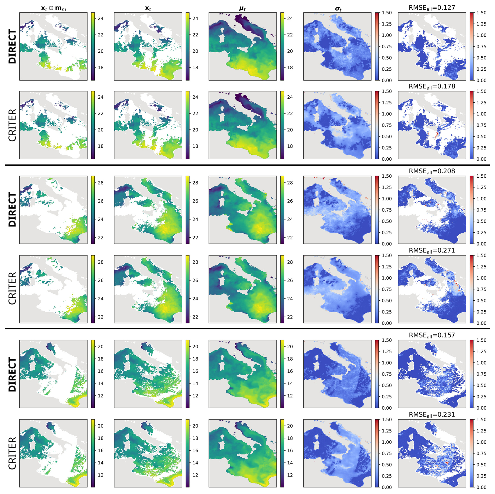
Figure A1 Comparison of DIRECT and CRITER reconstructions on the Mediterranean region. The columns show (from left to right): the partially observed input (x_t⊙m_m), the ground truth x_t, the reconstruction μ_t, the estimated uncertainty σ_t, and the absolute reconstruction error (RMSE_all). All values are in °C.

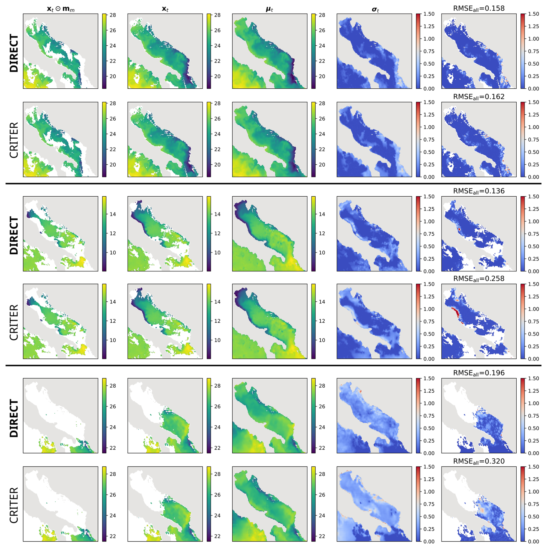
Figure A2 Comparison of DIRECT and CRITER reconstructions on the Adriatic region. The columns show (from left to right): the partially observed input (x_t⊙m_m), the ground truth x_t, the reconstruction μ_t, the estimated uncertainty σ_t, and the absolute reconstruction error (RMSE_all). All values are in °C.

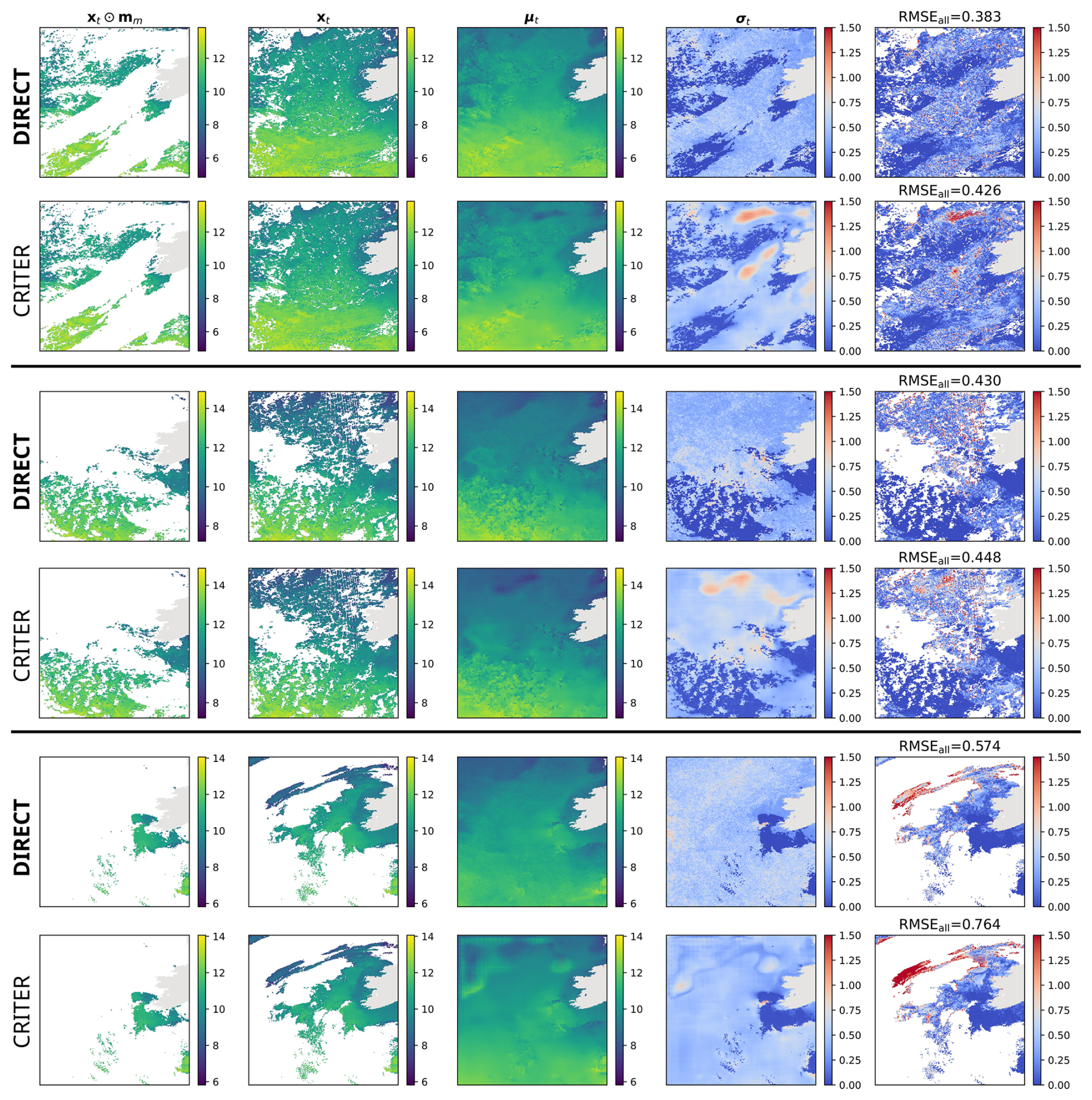
Figure A3 Comparison of DIRECT and CRITER reconstructions on the Atlantic region. The columns show (from left to right): the partially observed input (x_t⊙m_m), the ground truth x_t, the reconstruction μ_t, the estimated uncertainty σ_t, and the absolute reconstruction error (RMSE_all). All values are in °C.