GWSWEX v1.0: a dual-solver 1D unsaturated zone model for mass-conservative groundwater recharge and runoff computation in distributed hydrological modelling

Faithful numerical representation of the coupled groundwater (GW)–unsaturated-zone (UZ)–surface-water (SW) dynamics at regional scales is constrained by the structural extremes currently available: fully three-dimensional Richards-equation solvers resolve variably saturated flow rigorously but at a per-evaluation cost that forecloses ensemble calibration and multi-decadal projection, whereas conceptual bucket schemes cannot track a moving groundwater head, represent capillary rise, or impose a soil-moisture-dependent evapotranspiration (ET) stress. This study introduces GWSWEX (Groundwater–Surface Water EXchange), a vertically resolved, process-based UZ model designed to sit between an external GW model and an external SW model within an integrated modelling chain. Its principal innovations are two interchangeable solvers behind a single unified API: an explicit operator-split bucket-sequence solver with CFL-adaptive sub-stepping and an implicit mixed-form Richards solver with Picard linearisation, sharing the same Mualem–van Genuchten constitutive relations and piecewise-linear drainable-volume function for a freely moving groundwater head; the per-step storage budget closes to floating-point tolerance in the explicit solver and to a small, well-characterised residual in the implicit solver, enabling a coupled GW–UZ–SW iteration to converge without under-relaxation. Verification against HYDRUS-1D across six soil profiles under two contrasting forcing scenarios shows sub-centimetre to near-centimetre groundwater-head accuracy under smooth daily forcing, with eleven of twelve basic-scenario cases attaining an RMSE at or below the 2 cm discretisation step and a wet-phase mean RMSE of approximately 4 cm (implicit) and 8 cm (explicit) under intensive hourly forcing; an iterated one-at-a-time sensitivity analysis characterises the empirical parameters and the structural limits of the layered-bucket abstraction, while a parallel-ensemble benchmark shows both solvers completing a thousand-column ensemble six to twelve times faster than parallelised HYDRUS-1D, at sub-linear run-time scaling exponents of approximately 0.92–0.93 that render ensemble-grade calibration and multi-decadal projection tractable on mainstream consumer-grade hardware.

1 Introduction

The integrated representation of GW, UZ, and SW dynamics has been a recurring requirement of regional-scale hydrology since at least the foundational studies of Freeze (1972), and is now embedded in regulatory frameworks such as the EU Water Framework Directive (Bates et al., 2008; Barthel, 2014). Within this continuum the unsaturated zone occupies a distinctive position: it partitions precipitation between infiltration and runoff, governs the timing and magnitude of groundwater recharge, and controls the soil-moisture state on which actual evapotranspiration depends, thereby regulating both drought and flood signals as they propagate between the atmosphere, the river network and the aquifer (Beven, 2012; Clark et al., 2015a; Barthel and Banzhaf, 2016; Mensah et al., 2022; Banerjee and Ganguly, 2023; Moeck et al., 2024; Tsypin et al., 2025). Despite this central role, reviews of process representations in regional and Earth-system models continue to report the lower UZ–GW boundary as free or restricted drainage and the GW–SW exchange as poorly represented (Sophocleous, 2002; Clark et al., 2015a; Fan et al., 2019; Gleeson et al., 2021).

Two structurally distinct families of models bracket the present landscape. At one end, fully integrated 3-D Richards-class models (Kollet and Maxwell, 2006; Brunner and Simmons, 2012; Paniconi and Putti, 2015; Maxwell et al., 2015) resolve the variably saturated subsurface rigorously, but at a per-evaluation cost that, even with massive parallelism (Hwang et al., 2014), precludes the multi-decadal simulation, the Bayesian calibration, projection ensembles, and sensitivity studies that are routine elsewhere in the geosciences (Dogan and Motz, 2005; Farthing and Ogden, 2017); Beven (2019), building on observations dating to Beven (1989), further argues that, in many regional-scale contexts, the Richards equation is at once too detailed (over-weighting capillary forces) and not detailed enough (ignoring preferential and non-equilibrium flow; see also Beven and Germann, 2013). At the other end, the layered-bucket and conceptual schemes that underpin most regional integrated hydrological models achieve tractability at the cost of the vertical structure that faithful GW–UZ–SW coupling requires; they cannot represent a freely moving groundwater head as a prognostic state, capillary rise from a shallow water table into a depleting root zone, or an ET stress that responds to the local soil-moisture profile rather than a column average. The classification offered by Hrachowitz and Clark (2017) is a useful frame here: the requirement is for a process-based middle of the modelling spectrum, neither so reductive as to reduce to a calibrated water balance, nor so universal as to carry the full computational burden of a 3-D Richards solver.

A growing middle-ground literature (Bizhanimanzar et al., 2019, 2020; Burek et al., 2020; Brandhorst et al., 2021; Oad et al., 2025) and recent reviews of the GW–SW exchange landscape (Gupta and Kumar Sharma, 2023; Banerjee and Ganguly, 2023; Woessner, 2023; Ahmadi, 2024) confirm that the gap between integrated 3-D models and bucket-style conceptual models has narrowed but not closed; the reduced-order semi-continuum approaches now being explored for the unsaturated zone (Kmec et al., 2023) remain some distance from the integrated-modelling chains in which they would operate. What remains largely missing is an openly available, vertically resolved, process-based UZ component that simultaneously: (i) tracks a freely moving groundwater head within a layered, heterogeneous column and exposes it as a prognostic state to an external GW model; (ii) couples GW, UZ, and SW within a single mass-conservative framework; (iii) relies on physically interpretable constitutive relations rather than empirical surrogates; (iv) absorbs sharp atmospheric forcing without operator intervention through adaptive or unconditionally stable time-stepping; and (v) is element-parallel and computationally frugal enough for multi-decadal simulations, ensemble-grade calibration, projection, and sensitivity analyses. A second, equally consequential but less technical gap concerns reproducibility: barriers to source-code sharing and fragmented developer communities continue to limit the cumulative growth of the field (Clark et al., 2017); as Duethmann et al. (2020) illustrate, the community consequently struggles to explain why two well-regarded models diverge in their projections.

The reduced-order couplers closest to the present work occupy the same intermediate position, yet each stops short of the combination that GWSWEX assembles: conceptual unsaturated storages coupled to a saturated-zone solver under a hydrostatic-equilibrium assumption (Bizhanimanzar et al., 2019, 2020), a methodological 1-D Richards–Boussinesq coupling in an interpreted language (Brandhorst et al., 2021), an empirical drainage lower boundary calibrated against a 2-D reference (Oad et al., 2025), and the conceptual soil storage of an openly released regional and global model (Burek et al., 2020). A capability comparison against these couplers and against representative unsaturated-zone, integrated, and conceptual models (Table 1) situates the position that GWSWEX is designed to occupy, the detailed model-by-model assessment being deferred to Sect. 4.6.

Table 1 Capability comparison of GWSWEX with representative unsaturated-zone, integrated, and conceptual models.

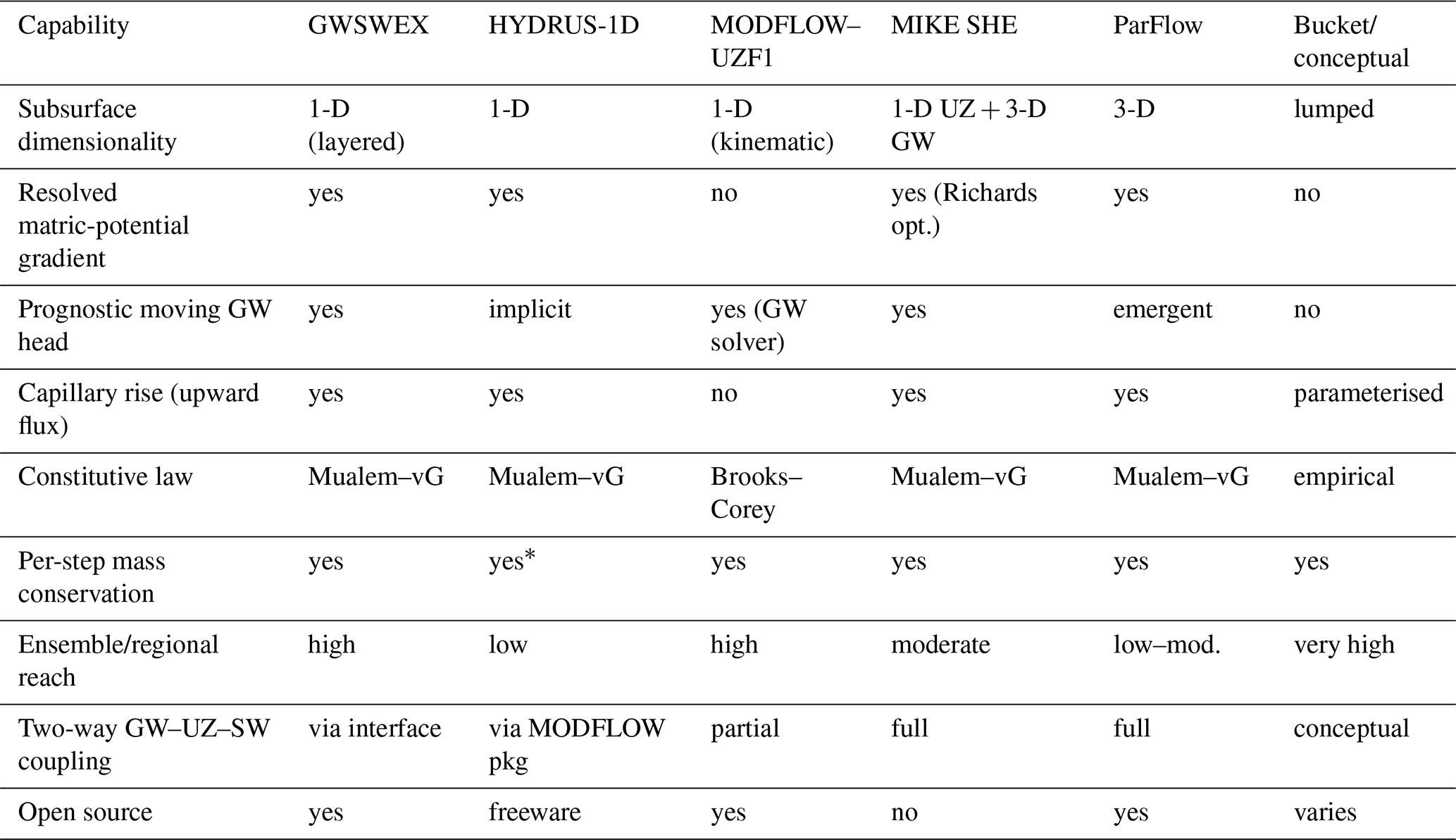
^* HYDRUS-1D conserves mass at converged Picard iterates but convergence is fragile in low-K_sat ponded columns.

This paper introduces GWSWEX (Groundwater–Surface Water EXchange), a vertically resolved, dual-solver UZ coupler designed to address both gaps. Section 2 presents the model concept and the verification, sensitivity, and performance methodology; Sect. 3 reports the results; Sect. 4 discusses them; Sect. 5 draws inferences from the findings. Appendix A carries the full model-physics; Appendix B the software architecture. The complete model code, input files, experiment-definition, and analysis notebooks are available in the open-source repository (Kootanoor Sheshadrivasan, 2026).

2 Methodology

GWSWEX Model description

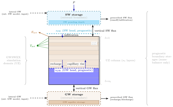
GWSWEX (Groundwater–Surface Water EXchange) is a vertically resolved, process-based UZ coupler. Its design philosophy is deliberately one of controlled compromise: rather than competing with fully three-dimensional Richards-class solvers on vertical-flux fidelity, it retains the matric-potential gradient and a prognostic moving groundwater head that conceptual bucket schemes discard, while preserving the per-element computational frugality, the physical interpretability of its constitutive relations, and the numerical robustness across forcing regimes that ensemble-grade regional application demands. Each model element is represented as a layered 1-D soil column with three prognostic storages: GW head, per-layer UZ storage, and SW (ponding) depth. The model is intended to sit between an external GW model and an external SW model in an integrated modelling chain, receiving lateral GW and SW exchange fluxes from those models as boundary conditions; all vertical fluxes (infiltration, gravity drainage, capillary redistribution, soil evaporation, root water uptake, recharge to GW, exfiltration to SW) are resolved internally and mass-conservatively at each step; Fig. 1 illustrates the column structure, the prognostic storage hierarchy, and the principal vertical and lateral flux pathways.

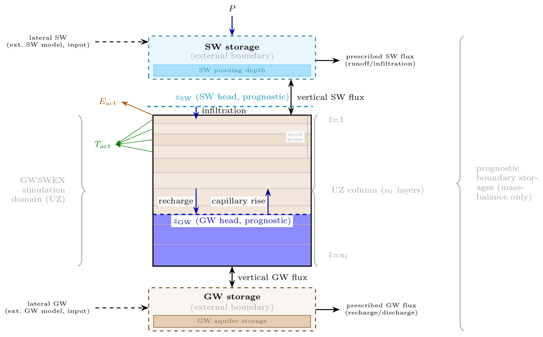
Figure 1 Column-element architecture of GWSWEX. Centre: layered UZ column (simulation domain). Top and bottom: prognostic SW and GW boundary storages. Dashed lines: prognostic SW head z_SW and GW head z_GW. Internal arrows: infiltration, recharge, capillary rise, surface evaporation E_act, and root-zone transpiration T_act (inter-layer gravity drainage and capillary redistribution omitted for clarity). Bidirectional outer arrows: aggregate column–storage exchange. Solid outward arrows from the storage boxes: prescribed SW and GW fluxes to coupled external models. Dashed arrows from the left: lateral SW and GW inputs.

The principal design choices are:

• Two interchangeable solvers behind a single API. The hydrological regime space encountered in a regional coupled domain is too broad for any single 1-D solver to cover with uniform fidelity: infiltration-dominated wet phases with sharp wetting fronts and surface ponding demand a numerically robust scheme under near-saturated conditions, while extended drought and deep-water-table recession phases demand a scheme that can advance over long time steps without instability. An explicit operator-split bucket-sequence solver with CFL-adaptive sub-stepping addresses the former; an implicit mixed-form Richards solver with Picard linearisation and Thomas-algorithm tridiagonal inversion addresses the latter. Both are offered as peers behind a single model API, share the same vertical discretisation, the same Mualem–van Genuchten constitutive relations (Mualem, 1976; van Genuchten, 1980), and the same coupling interface; the complete numerical formulations are in Appendix A.

• Freely moving groundwater head in a layered, heterogeneous column. Each element is discretised into an arbitrary number of layers, each with its own van Genuchten parameters, and the groundwater head is recovered from a piecewise-linear drainable-volume function that integrates layer-specific yield across material boundaries, permitting full vertical heterogeneity in a mass-conservative and analytically invertible formulation.

• Soil-moisture-dependent ET partitioning. Both solvers apply a Laio-type four-saturation-threshold stress function (Laio et al., 2001) to partition potential evaporation and transpiration into actual fluxes at each step. The implicit solver evaluates the actual demand at each Picard iterate, so that the sink responds to the head profile being solved for; the explicit solver evaluates it after gravity drainage but before capillary redistribution, reflecting the timescales at which these processes operate.

• Strict per-step mass conservation for robust iterative coupling. The per-step storage budget closes to floating-point tolerance in the explicit solver and to a small, well-characterised residual in the implicit solver, so that the outer GW–UZ–SW coupling iteration can converge without additional under-relaxation.

• Modular Modern Fortran kernel with a Python API. The per-element independence of the column physics is exploited via OpenMP work-sharing across elements; the user-facing layer is a Python package that provides Pydantic-validated configuration, NetCDF I/O, checkpointing, and the lateral coupling interface (Appendix B).

GWSWEX targets the class of regional integrated modelling problems in which the UZ must be represented faithfully, with vertically resolved storage, a moving groundwater head, and mass-conservative flux accounting, at a per-element computational cost low enough for ensemble calibration, sensitivity studies, and multi-decadal projections on consumer-grade hardware. Fully integrated 3-D Richards-class models retain their structural advantage wherever the three-dimensional transient solution is the governing concern; the gap they leave at the regional-ensemble end of the spectrum is the design space GWSWEX is built to fill.

2.1 Groundwater head and soil moisture simulation accuracy

The evaluation reported here is a code-to-code verification rather than a field validation: it isolates the numerical fidelity and per-step mass conservation of the two solvers under controlled synthetic forcing with perfectly known parameters and boundary conditions, thereby separating the behaviour of the numerical schemes from the atmospheric, parameter, and boundary uncertainties that a field comparison would introduce; a verification against measured field data is the natural successor experiment, as discussed in Sect. 4.4.

The verification compares the explicit and implicit GWSWEX solvers against HYDRUS-1D (Šimůnek et al., 2008) as a representative iterative implicit Richards-equation reference for vertical 1-D variably saturated flow at the column scale. HYDRUS-1D is configured through the phydrus Python wrapper (Collenteur et al., 2021) (v0.2.0, modified for Python 3.9 onwards; https://github.com/veethahavya-CU-cz/phydrus, last access: 2 September 2026) with its native Feddes ET stress function (Feddes et al., 1978); per-case input files, experiment definitions and comparison notebooks accompany the open-source repository (Kootanoor Sheshadrivasan, 2026).

The choice of HYDRUS-1D over a saturated-zone model with a UZ package (e.g. MODFLOW–UZF, MODFLOW–SWB) or a fully integrated model (e.g. MIKE SHE, ParFlow) follows from the scope: since GWSWEX is introduced here as a 1-D UZ component intended for coupling to external GW and SW models rather than as an integrated solver, the verification must isolate per-column physics from any particular saturated-zone formulation. HYDRUS-1D is the natural reference for both GWSWEX solvers. For the implicit solver the case is direct: HYDRUS-1D is a standalone column code solving the same 1-D mixed-form Richards equation under the same Mualem–van Genuchten constitutive relations, making it a like-for-like reference for constitutive physics, ET partitioning and capillary-rise representation. For the explicit solver the two GWSWEX solvers share the same constitutive relations, column geometry and layering, forcing, and boundary-condition specification, so the explicit solver is benchmarked against the same physically faithful column reference as its implicit peer, the residual isolating the cascade abstraction rather than any constitutive mismatch; and HYDRUS-1D is the most widely used and widely cited software for unsaturated-zone modelling, with a long and proven track record as the community reference standard against which new UZ schemes are routinely compared. A downstream coupled-modelling demonstration against an integrated GW–UZ–SW reference is the natural successor experiment and is signalled in Sect. 4.5.

Two forcing setups probe complementary regimes, each acting as a stress-test intended for evaluating the models. The basic setup is a 65 d, daily-interval experiment with a 5 d warmup, 30 d wet phase and 30 d dry phase on a 3 m column (n_l=150, Δz=0.02 m), groundwater head initialised at 1.5 m depth and a root zone growing linearly from 0.05 to 0.60 m. Wet-phase precipitation is tuned per soil to raise the groundwater head substantially without surface ponding, probing the slow-recharge, deep-GWH, capillary-fringe regime that dominates field-scale water budgets and exercising the gravity-drainage and ET-driven capillary-recession behaviour of both solvers under smooth daily forcing. The intensive setup is a 32 d, hourly-interval experiment with warmup/wet/dry/cooldown windows of 72/240/288/168 h on a 1.5 m column (n_l=150, Δz=0.01 m), groundwater head initialised at 1.20 m depth and a fixed 0.60 m root zone. Wet-phase precipitation is just high enough to drive the groundwater head to the surface and produce ponding, probing the saturation-excess regime (Dunne and Black, 1970) in which sustained recharge raises a shallow water table to meet the surface rather than the infiltration-excess mechanism (Horton, 1933) of a deep water table under rainfall exceeding surface K_sat (confirmed mechanistically in Sect. 4.1), and exercising the dynamic top-boundary switching of the implicit solver and the saturated-column branch of the explicit solver. For this setup, HYDRUS-1D is likewise run with the atmospheric boundary condition's surface-reservoir option enabled, so that ponded water accumulates there as a genuine state variable rather than being shed as runoff, making its peak-ponding and ponded-duration diagnostics directly comparable to GWSWEX's explicit SW store; the basic setup instead uses the runoff-shedding option, which is immaterial there because ponding does not occur by construction.

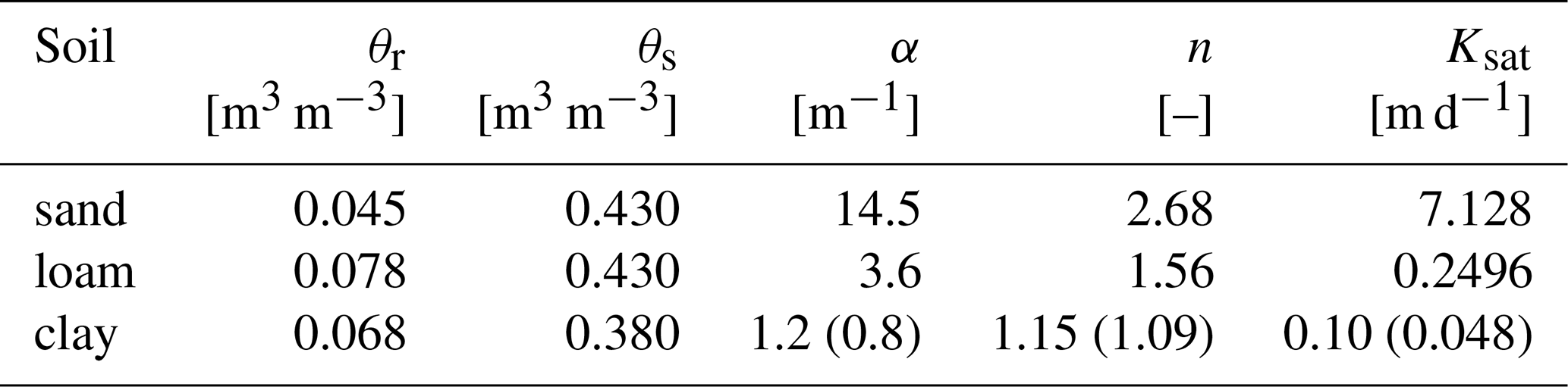
Each setup is run on six soil profiles drawn from the Carsel and Parrish (1988) catalogue: the three single-material columns sand, loam, and clay; and the three layered profiles sand-over-loam, sand-over-clay, and loam-over-clay. Per-soil precipitation and reference-ET rates are scaled so that the nominal GWH amplitude is comparable across soils despite the order-of-magnitude differences in K_sat between the catalogue endpoints. The clay van Genuchten parameters are relaxed slightly toward loam (Table 2, originals in parentheses) because the catalogue defaults render basic-clay unresponsive on a 65 d horizon; the relaxed clay remains the lowest-K_sat soil in the catalogue by an order of magnitude, and the relaxation is applied uniformly to both solvers. The full configuration is summarised in Tables 2, 3, and 4.

Table 2 van Genuchten–Mualem hydraulic parameters of the three constituent soils. The clay row carries the relaxation toward the loam end of the catalogue described in the text; the original Carsel–Parrish values are given in parentheses for the three relaxed parameters. The Mualem pore-connectivity parameter λ=0.5 for all three soils.

The two layered profiles partition the column from the surface downward as follows: sand-over-loam carries sand over the upper one third and loam below; sand-over-clay carries sand over the upper two thirds and clay below; loam-over-clay carries loam over the upper two thirds and clay below.

Table 3 Spatial domain, vertical discretisation, groundwater-head initialisation, root-zone schedule and phase windows of the basic and intensive setups.

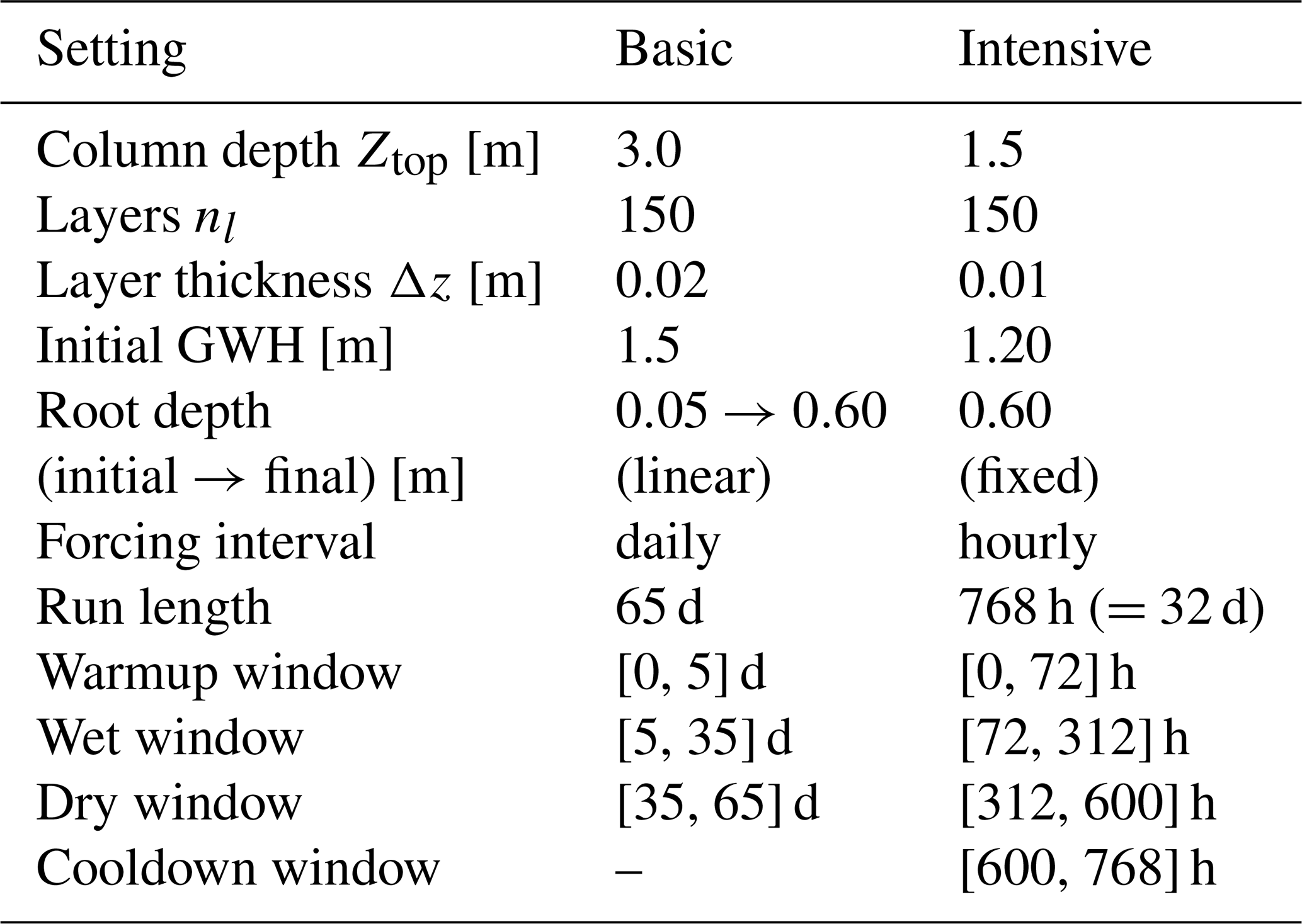
Table 4 Per-soil constant atmospheric forcing rates (precipitation P, potential bare-soil evaporation E_p, potential transpiration T_p) imposed in the wet and dry windows of each setup. Basic-setup rates are in cm d⁻¹; intensive-setup rates are in mm h⁻¹.

For each of the twenty-four (soil × setup × solver) cases, the comparison notebooks produce the GWH time series and its residual against HYDRUS-1D; zone-averaged saturation in four physically meaningful depth intervals (root zone, transmission zone, capillary fringe, and full UZ); soil-moisture profile snapshots at the phase transition times; cumulative actual evaporation and transpiration; cumulative precipitation, infiltration, and runoff; and the cumulative intrinsic mass-balance residual. The primary scalar score is the GWH RMSE against HYDRUS-1D over the full simulation horizon, with the Nash–Sutcliffe efficiency (Nash and Sutcliffe, 1970) reported as a secondary score. The same RMSE and NSE are also computed separately for the wet and dry phases of each setup (basic: wet [5, 35] d, dry [35, 65] d; intensive: wet [72, 312] h, dry [312, 600] h, warmup and cooldown excluded), so that the gravity-drainage and the ET/capillary-rise branches of the model can be diagnosed independently. HYDRUS-1D returns NaN for the GWH diagnostic during ponded sub-intervals (no sign change in the head profile inside the column) and is clipped at the surface (≥0 cm) before any comparison; these timesteps are masked from all RMSE and NSE computations. GWSWEX folds ponded water into surface storage rather than into the GWH diagnostic, so its GWH trajectory is physically defined throughout and is likewise clipped at the surface for visual consistency.

2.2 Sensitivity analysis

The sensitivity of the GWSWEX groundwater-head trajectory to the empirical parameters of the two solvers was investigated through an iterated one-at-a-time (OAT) coordinate-descent calibration carried out for every (soil, setup, solver) cell. An OAT design is an axis-aligned local screening protocol whose strengths and limits relative to variance-based global designs are well established (Saltelli and Annoni, 2010; Razavi and Gupta, 2015; Pianosi et al., 2016); it is adopted here for its physical interpretability across twenty-four cells and its tractable per-cell budget, with the inferential constraints discussed in Sect. 4.2. The full per-case calibrated configurations and supporting discussion are provided with the open-source repository.

For each of the twenty-four cells, the parameters of Table 5 were varied independently through a discrete grid whose levels were chosen by physical bracketing rather than uniform sub-division.

Table 5 OAT parameter sweep grid. Green–Ampt and ET-stress parameters apply to both solvers; remaining parameters are solver-specific. Scoring: wet, dry, dry + cool are phase-windowed GWH RMSE; overall is full-run RMSE (physical rationale in the text). Laio thresholds satisfy $s_{\mathrm{h}}\le s_{\mathrm{w}}\le s_{\mathrm{e}}\le s^{*}\le \mathrm{1}$.

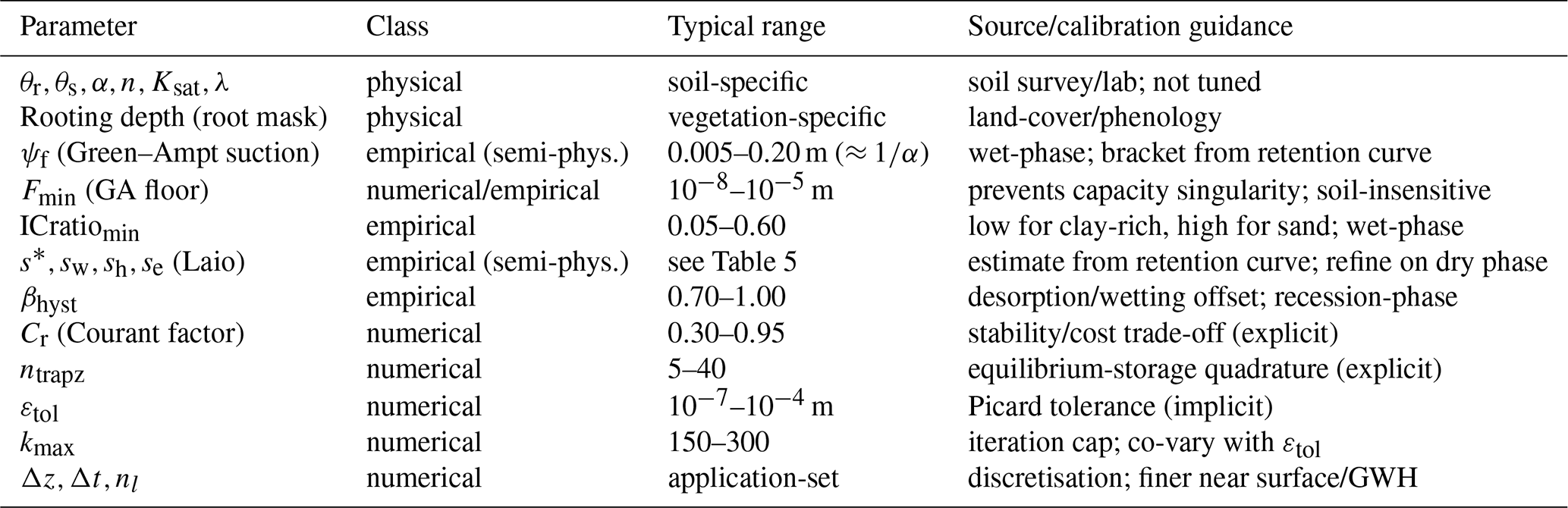
The model parameters fall into three classes that the user should treat differently in practice. The constitutive parameters of the Mualem–van Genuchten relations and the rooting depth are physically based, and are measured or transferred from soil and vegetation surveys rather than tuned; the infiltration, inter-layer-connectivity, ET-stress and hysteresis parameters are empirical or semi-physical parameters whose plausible ranges are bracketed by the retention curve and whose optima are mildly soil-dependent; the Courant safety factor, the equilibrium-storage quadrature resolution, and the Picard convergence controls are purely numerical, set for stability and computational cost rather than to represent a physical process. Table 6 summarises this classification together with a typical range and a calibration note for each parameter.

Table 6 Classification of GWSWEX parameters with typical ranges and calibration guidance.

Acceptance in the coordinate-descent procedure is evaluated against a phase-targeted metric rather than a single whole-run RMSE: each parameter family is active in a specific portion of the simulation, and is therefore scored against the phase RMSE that exercises it (Table 5, rightmost column). The Green–Ampt and inter-layer connectivity parameters govern infiltration and wetting-front propagation and are scored against wet-phase RMSE; the Laio thresholds govern dry-phase ET partitioning and capillary rise and are scored against dry-phase RMSE; the explicit hysteresis blend β_hyst modulates the desorption branch traversed during recession and is scored against the combined dry-plus-cooldown RMSE; the Picard convergence controls, the Courant safety factor C_r and the equilibrium-storage quadrature resolution n_trapz act throughout and are scored against full-run RMSE. Convergence termination always uses overall RMSE: descent terminates when the overall RMSE does not improve by at least 0.5 % within a pass or after a maximum of three passes. The per-parameter acceptance threshold is τ_accept=0.02 for the basic setup and 0.05 for the intensive setup, expressed as a fraction of the current best value of the targeted phase metric; the asymmetric margin reflects the larger trial-to-trial variance in the intensive case driven by sharper GWH movement and surface ponding events.

The constitutive functions, the form of the ET stress function (Laio for GWSWEX, Feddes for HYDRUS-1D, neither tuned), the root-growth schedule, and the spatial and temporal discretisations are held fixed across the entire study. The Laio thresholds $\mathit{\{}{s}^{*},s_{\mathrm{w}},s_{\mathrm{h}},s_{\mathrm{e}}\mathit{\}}$ are treated as calibratable parameters because they are practically dependent on the nature of soil and vegetation. The limitations of the iterated OAT design itself are discussed in Sect. 4.2.

2.3 Computational performance benchmark

The benchmark addresses how the run-time of each code grows with the number of independent catchment elements. Four ensemble sizes are tested, $n_{\mathrm{e}}\in \mathit{\{}\mathrm{1},\mathrm{10},{\mathrm{10}}^{\mathrm{2}},{\mathrm{10}}^{\mathrm{3}}\mathit{\}}$, with each element an independent 1-D column under identical geometry, materials, initial conditions and forcing.

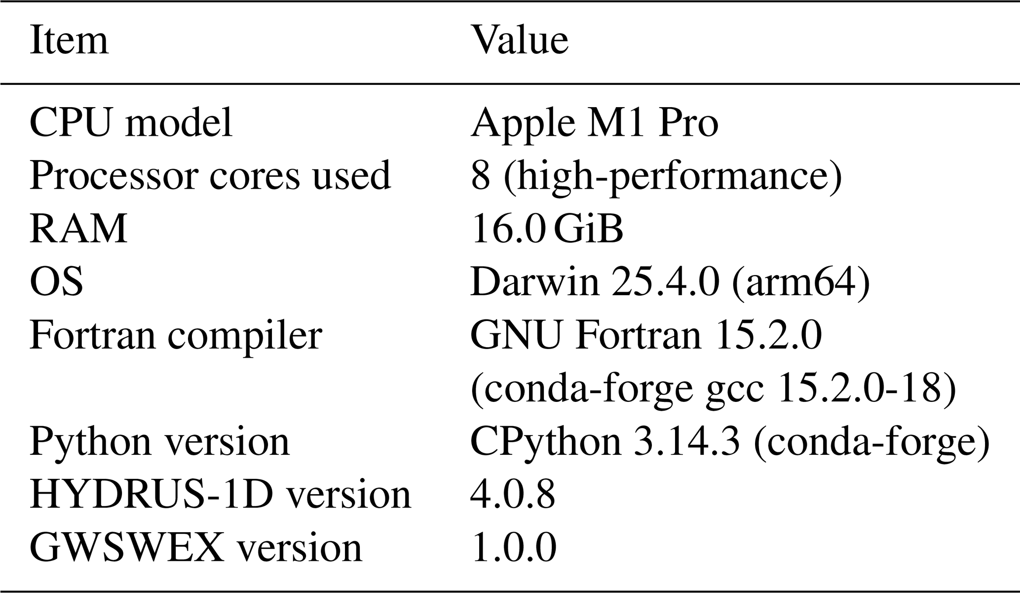
HYDRUS-1D simulates one column at a time (Šimůnek et al., 2008), so for n_e>1 the columns are distributed across 8 worker processes from a shared queue. GWSWEX runs all n_e columns simultaneously across 8 cores via OpenMP. Both configurations use the same 8 high-performance cores of an Apple M1 Pro (the 2 remaining low-power cores are excluded because mixing them into a tightly synchronised parallel loop introduces idle waiting at each synchronisation point). The full machine configuration is summarised in Table 7.

Table 7 Hardware and software environment for the computational performance benchmark.

The benchmark uses the intensive-sand-loam profile (Table 2), 32 simulated days at hourly macro-step (N=768 steps), with the same forcing as the verification experiment (Kootanoor Sheshadrivasan, 2026). The profile choice preserves direct continuity with the single-element accuracy comparison in Sect. 3.1 and exercises both material layers in physically distinct regimes: the sand upper layer drives rapid gravity drainage, while the loam lower layer presents the slower capillary dynamics that govern GWH recession.

The measured time covers initialisation, time-stepping and output for each code. For each (n_e, code) combination, three independent trials were executed; the reported time is the median elapsed run-time, with the inter-trial range reflecting trial-to-trial variability. Recorded metrics are: total elapsed run-time τ(n_e) [s]; total processor time summed across cores [s]; peak working memory [MiB]; and total output written [MiB]. An empirical scaling exponent β is estimated from a log–log fit, $\log \mathit{\tau }=\mathit{\beta }\log n_{\mathrm{e}}+\log a$, over n_e≥10; β=1 indicates run-time proportional to ensemble size, β<1 that each additional column costs proportionally less than the last as the fixed parallel-setup cost is shared across more columns. Benchmark scripts accompany the open-source repository.

3 Results

3.1 Groundwater head and soil moisture simulation accuracy

Groundwater-head accuracy. Table 8 reports the GWH RMSE and NSE of GWSWEX against HYDRUS-1D for each of the twenty-four (soil × scenario × solver) simulations, and Figs. 2 and 3 plot the corresponding trajectories, demonstrating GWH rise under wet-phase gravity drainage and recession under dry-phase evapotranspiration and capillary-rise feedback across contrasting soil hydraulic regimes. Across the basic scenario, eleven of twelve simulations attain GWH RMSE ≤2 cm and NSE ≥0.85, capturing the daily-interval trajectory to within the discretisation step (Δz=2 cm). The intensive-scenario residuals are larger and concentrated in the simulations dominated by a low-K_sat clay layer; the intensive-sand and intensive-sand-over-loam HYDRUS-1D references additionally truncate prematurely under solver nonconvergence, with the corresponding dry-phase entries in Fig. 5 marked “n/a”. The physical and numerical origins of these residuals and truncations are examined in Sect. 4.4.

Table 8 End-to-end GWH RMSE [cm] and NSE of GWSWEX against HYDRUS-1D, full simulation horizon.

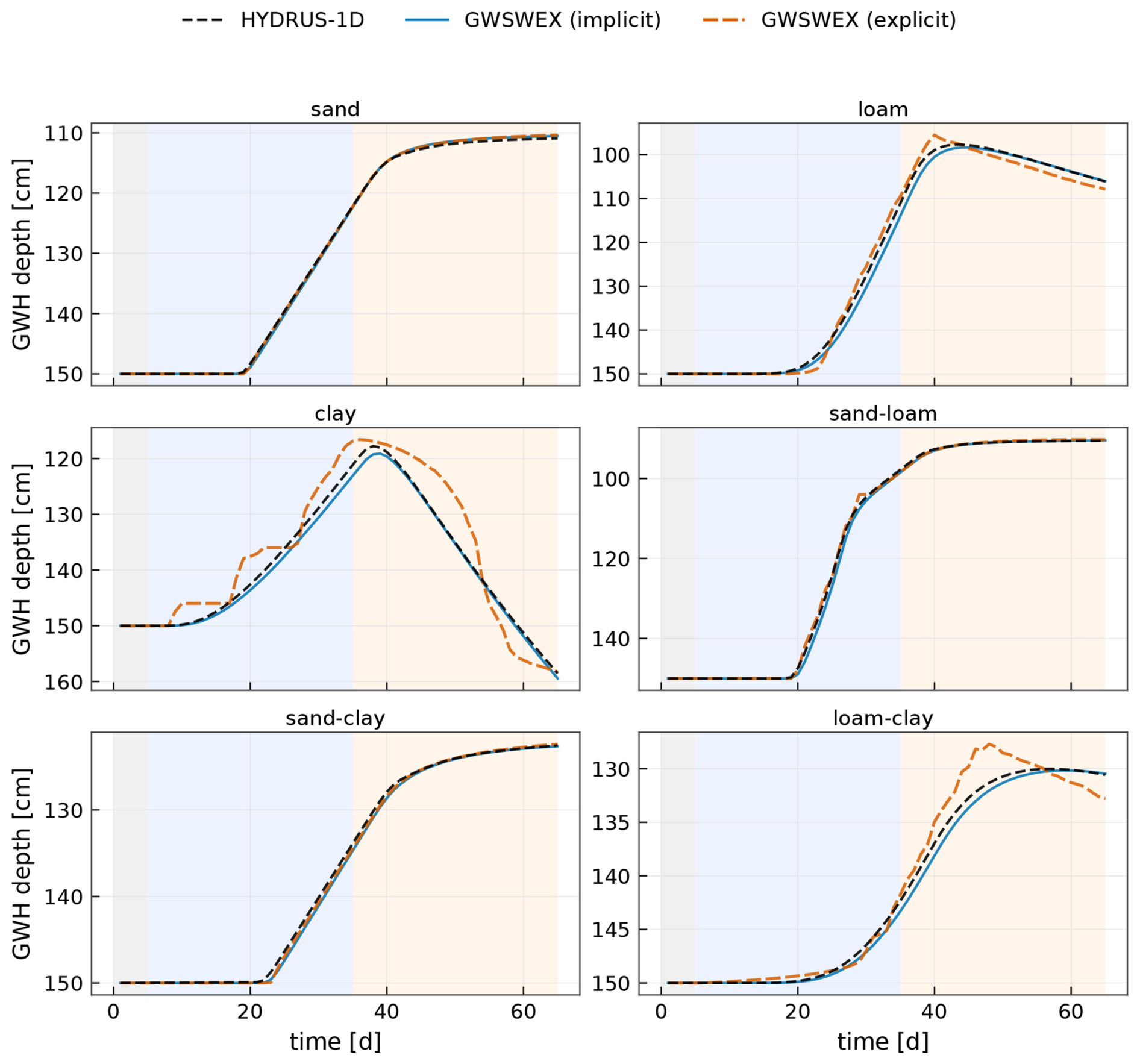
Figure 2 Simulated GWH trajectories for the basic scenario (daily, 65 d); one row per soil. HYDRUS-1D reference overplotted with GWSWEX implicit and explicit traces; shading marks warmup, wet, and dry phases; depth axis inverted. The wet-phase rise tracks the gravity-drainage mass partition and the dry-phase recession the ET-driven capillary demand on the saturated zone, the two solvers bracketing the HYDRUS-1D reference across the soil-hydraulic range.

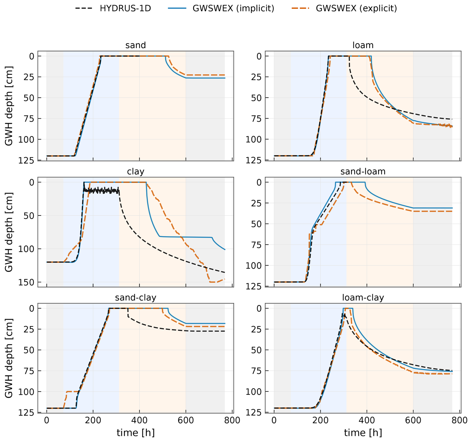
Figure 3 Simulated GWH trajectories for the intensive scenario (hourly, 768 h); one row per soil. HYDRUS-1D reference overplotted with GWSWEX implicit and explicit traces; shading marks warmup, wet, dry, and cooldown phases; depth axis inverted. The wet-phase rise tracks the gravity-drainage mass partition and the dry-phase recession the ET-driven capillary demand on the saturated zone, the two solvers bracketing the HYDRUS-1D reference across the soil-hydraulic range.

The per-step internal mass-balance residual closes to floating-point tolerance for the explicit solver away from cap events. For the implicit solver the cumulative residual is small: of order 0.2 cm on the basic-loam reference (per-step maximum approximately 0.5 cm), comparable to HYDRUS-1D itself and arising principally from the start-of-step evaluation of boundary fluxes.

Hydrological process metrics. Figure 4 resolves each (soil, scenario, source) simulation into three process-level metrics (wet-phase GWH rise with lag-to-peak in the intensive scenario; peak surface ponding and ponded duration; signed dry-phase GWH recession rate), and Fig. 5 splits each simulation's GWH-RMSE between the wet phase, the dry phase and the full horizon excluding warmup and cooldown. The wet-phase rise agrees across all twenty-four simulations to within or close to the discretisation step. In the intensive scenario, both GWSWEX solvers report higher peak ponding and longer ponded duration than HYDRUS-1D in the four simulations where HYDRUS completes the full horizon (loam, clay, sand-over-clay, loam-over-clay); this difference is a structural consequence of how the two codes partition the post-saturation net atmospheric flux between surface-storage accumulation and continued surface infiltration feeding the internal evapotranspiration sinks, as analysed in Sect. 4.1. For intensive-sand and intensive-sand-over-loam the HYDRUS reference terminates mid-run, so the apparent ponded-duration excess in those panels reflects coverage rather than a model difference. The dry-phase recession matches HYDRUS to tenths of $\mathrm{cm}/\mathrm{d}$ across the basic scenario but is under-estimated by GWSWEX by approximately 25 %–30 % in the most demanding clay-bearing intensive simulations. The mechanisms behind these patterns are discussed in Sect. 4.1.

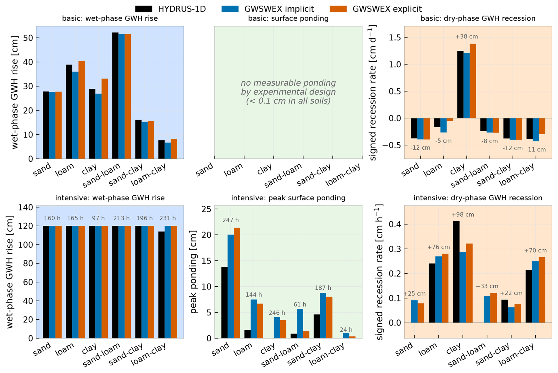
Figure 4 Per-simulation hydrological-process metrics; rows: basic (top) and intensive (bottom); columns: wet-phase GWH rise (left), peak surface ponding (middle), signed dry-phase GWH recession rate (right, positive = deepening). Bars per soil compare HYDRUS-1D, GWSWEX implicit, and GWSWEX explicit. Annotations: mean lag-to-peak (intensive wet-rise), mean ponded duration above 0.1 cm (intensive ponding), and mean signed dry-phase GWH change (recession). The ranking of wet-phase rise reads off the soil-hydraulic structure, while the dry-phase recession is positive (deepening) only where wet-phase moisture is retained in the upper zones and met by capillary rise from the groundwater head, as in clay.

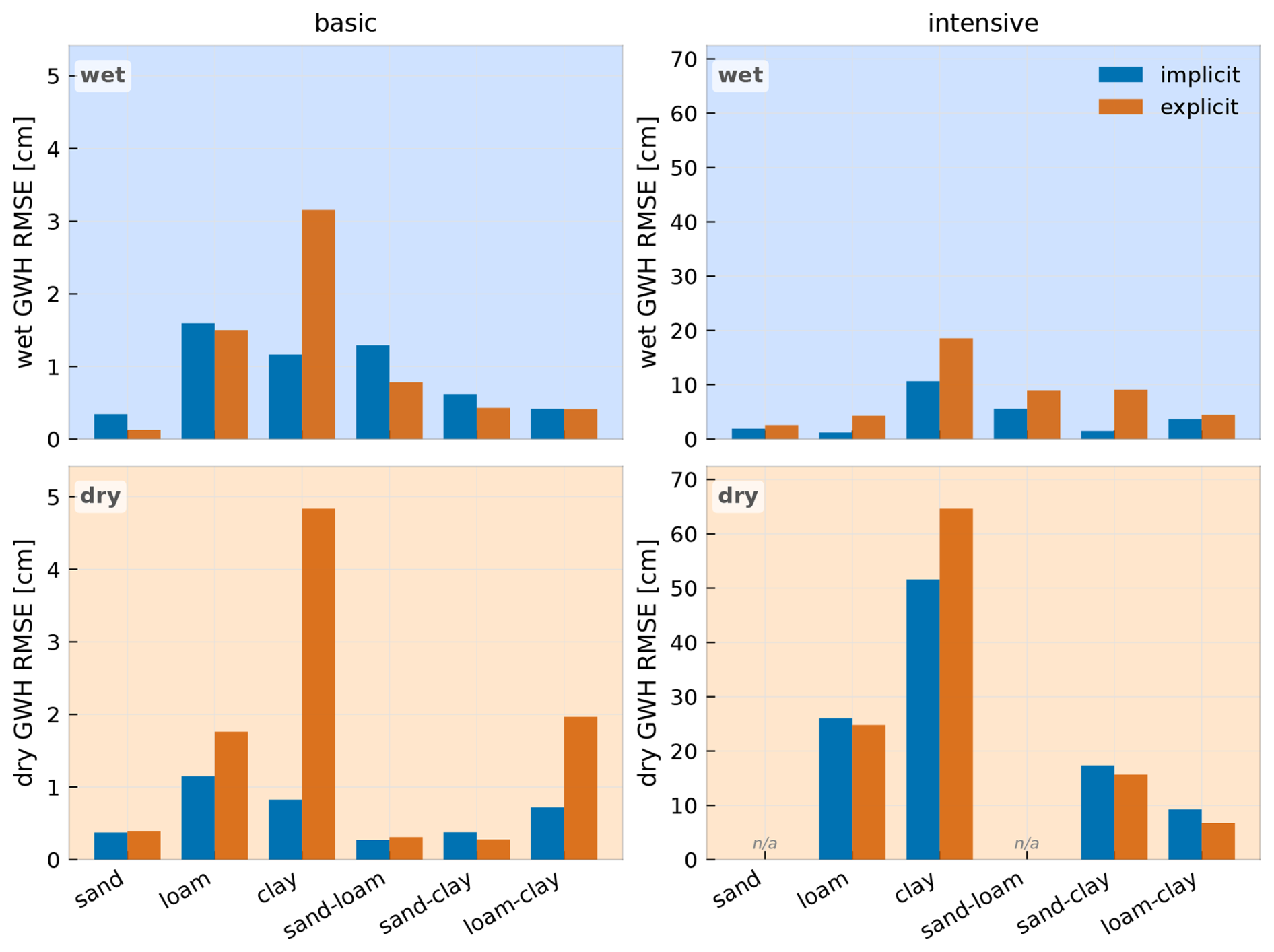
Figure 5 Phase-resolved GWH RMSE [cm] of GWSWEX against HYDRUS-1D by soil profile; rows: wet phase (top), dry phase (bottom); columns: basic scenario (left), intensive scenario (right). Cells marked “n/a” denote HYDRUS-1D truncation under nonconvergence. The wet-phase errors are uniformly small, locating the principal GWSWEX–HYDRUS divergence in the dry-phase ET and capillary-rise branch of the low-K_sat intensive profiles.

Vertical soil moisture distribution. Figures 6 and 7 report zone-averaged volumetric water content for each scenario. Figure 6 traces the downward propagation of infiltrated water through each depth zone and the response of the capillary fringe to GWH dynamics across the wet and dry phases; Fig. 7 contrasts the rapid wetting–drying cycles in the root zone with the slower transmission-zone response that mirrors the GWH trajectory, and the column-mean trace therein confirms storage conservation on the macro-step scale. By design, the basic forcing briefly saturates the UZ at the onset of the dry phase without sustained ponding, while the intensive forcing produces episodic ponding in the lower-K_sat profiles; both GWSWEX solvers reproduce this regime separation. The largest GWSWEX–HYDRUS departures concentrate in the deeper zones of the low-K_sat intensive simulations (intensive-clay, intensive-loam-over-clay, intensive-sand-over-clay), where the cascade reproduces the wet-phase saturation of the deeper zone but recedes more slowly through the dry phase. Column-internal mechanisms behind these signatures are interpreted in Sect. 4.1.

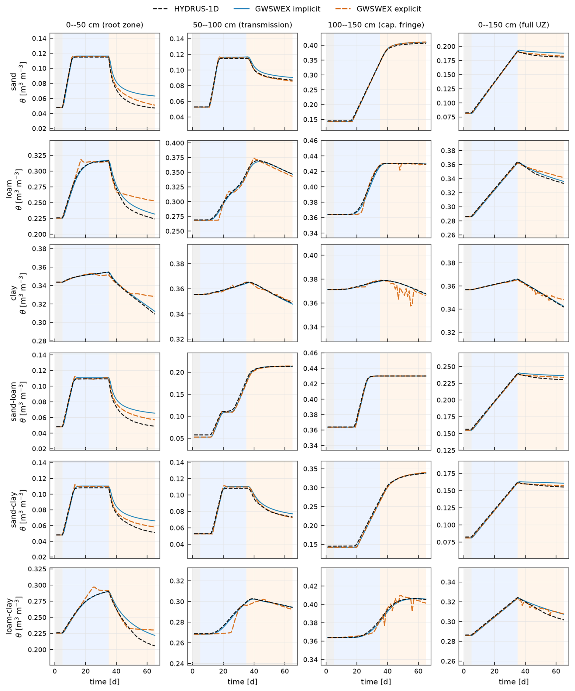
Figure 6 Zone-averaged volumetric water content θ (m³ m⁻³) for the basic scenario; rows: six soil profiles; columns: root zone (0–50 cm), transmission zone (50–100 cm), capillary fringe (100–150 cm), full-UZ mean (0–150 cm). Shading marks warmup, wet, and dry phases. The root zone tracks the daily forcing pulses, the transmission zone responds with a one- to three-day delay, the physical origin of the negative basic-scenario dry-phase recession rates, and the capillary fringe carries the slow monotone groundwater-head signal.

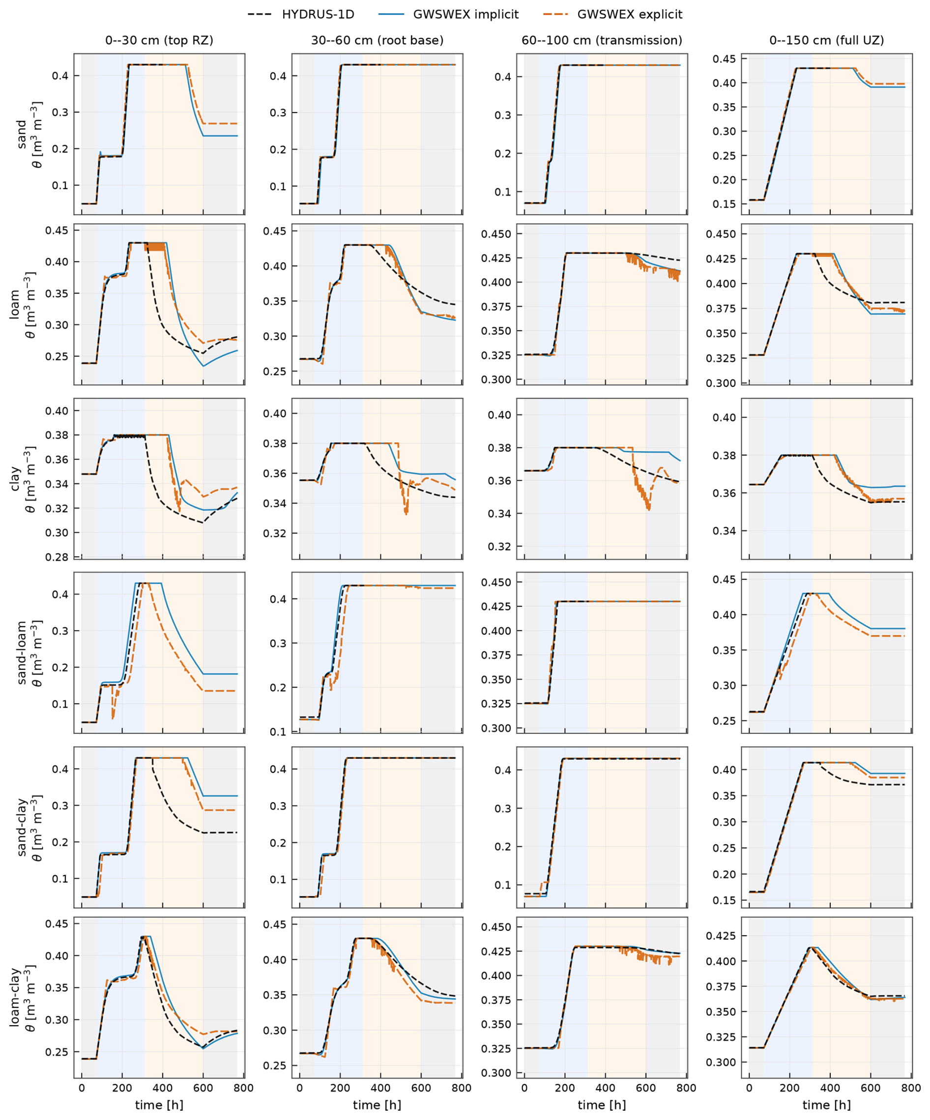
Figure 7 Zone-averaged θ (m³ m⁻³) for the intensive scenario; columns: top root zone (0–30 cm), root base (30–60 cm), transmission zone (60–100 cm), full-UZ mean (0–150 cm). Shading as in Fig. 6. The upper zones cycle hourly with the forcing while the deeper transmission zone follows the groundwater head; the largest GWSWEX–HYDRUS departures concentrate in the deeper zones of the low-K_sat profiles, localising the residual to the saturated–unsaturated capillary coupling, and the full-UZ mean confirms storage conservation on the macro-step scale.

3.2 Sensitivity of groundwater head dynamics to process parameterisation

Figure 8 summarises the per-parameter outcome of the OAT campaign as a heatmap of per-axis improvement in overall GWH RMSE for each simulation, expressed as a percentage of the pre-tuning baseline and ordered by sweep acceptance. Parameters are grouped left-to-right into wet-targeted (ICratio_min, ψ_f, F_min), dry-targeted (s^*, s_w, s_h, s_e, β_hyst) and numerical (C_r, n_trapz, ε_tol, k_max) families; rows are ordered solver × soil with the implicit block above the explicit block. Blank entries were either swept and rejected or are outside the solver-specific parameter set. The phase-targeted attribution is best read against Fig. 5; the per-family interpretation, the physical role of each parameter, and the inferential constraints of the OAT design are deferred to Sect. 4.2.

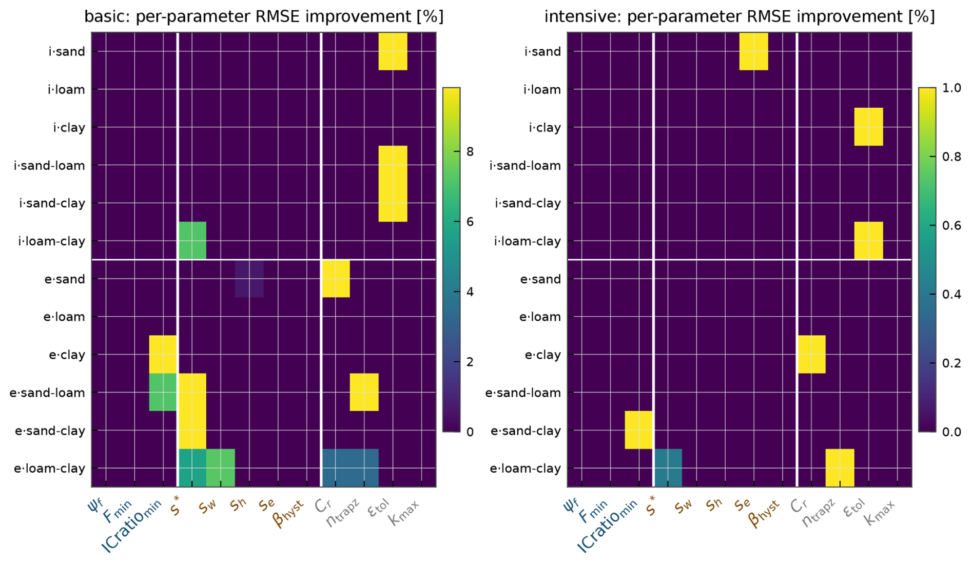
Figure 8 Per-parameter percentage reduction in overall GWH RMSE attributable to each accepted OAT adjustment. Columns: basic (left), intensive (right). Rows: solver × soil, implicit block above explicit block. Parameter groups (left to right, white dividers): wet-phase-active controls (infiltration, inter-layer connectivity), dry-phase-active controls (ET stress thresholds, hysteresis), numerical controls. Blank entries: swept-and-rejected or outside the solver-specific parameter set.

3.3 Computational performance

The benchmark protocol of Sect. 2.3 is applied across four ensemble sizes $n_{\mathrm{e}}\in \mathit{\{}\mathrm{1},\mathrm{10},{\mathrm{10}}^{\mathrm{2}},{\mathrm{10}}^{\mathrm{3}}\mathit{\}}$ for HYDRUS-1D and both GWSWEX solvers, each using 8 parallel cores. Median elapsed run-time, peak RAM and total disk output are reported in Table 9, and the corresponding scaling curves in Fig. 9.

Table 9 Median elapsed run-time τ [s] (three trials; range = min..max), total processor time [s] (summed across all cores), peak working memory (RAM) [MiB] and total output written to disk [MiB] for each code and ensemble size n_e.

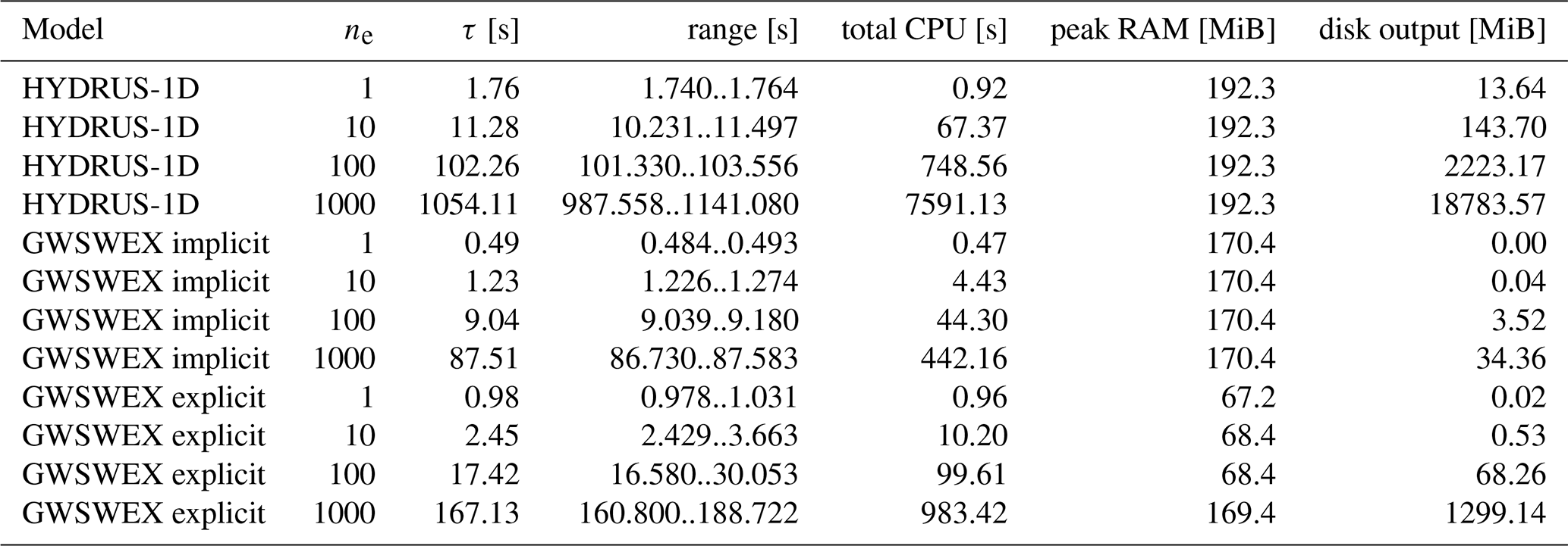
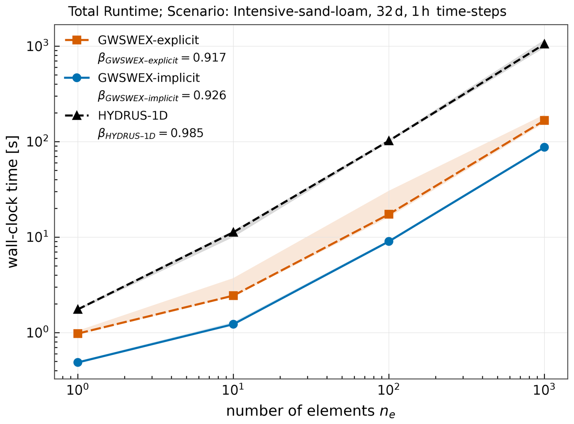
Figure 9 Total elapsed run-time τ(n_e) on log–log axes for HYDRUS-1D (8 parallel workers) and the GWSWEX solvers (8 parallel cores) on the intensive-sand-loam profile. Points: trial medians; shaded bands: trial min–max. Dashed annotations: power-law scaling exponent β fitted over n_e≥10.

At the single-column scale both GWSWEX solvers complete the 32 d, 768-step intensive sand-loam run faster than HYDRUS-1D, and at the largest tested ensemble (n_e=1000) the contrast widens by an order of magnitude. HYDRUS-1D's run-time at large n_e is dominated not by physics computation but by text-format output: at n_e=1000 the 8 parallel workers collectively produce approximately 18.4 GiB of plain-text result files and queue behind each other for disk access, so total run-time climbs roughly five-fold relative to the single-column case even though physics computation itself scales sub-linearly. GWSWEX holds intermediate state in working memory and writes output two to three orders of magnitude more compactly, so its run-time scales with physics rather than disk throughput. The explicit-to-implicit run-time ratio of approximately 1.9 reflects the additional sub-steps the CFL stability criterion forces in the sand layer. All three configurations make near-full use of their cores (utilisation approximately 90 %, 63 % and 73 % for HYDRUS-1D, GWSWEX implicit and GWSWEX explicit respectively); working memory is modest throughout.

The run-time scaling exponents from log–log power-law fits over $n_{\mathrm{e}}\in \mathit{\{}\mathrm{10},\mathrm{100},\mathrm{1000}\mathit{\}}$ are reported in Table 10. All three are below 1; HYDRUS-1D's exponent of 0.985 is indistinguishable from linear because its disk-output volume grows in direct proportion to n_e and is not absorbed by the parallelism, whereas the GWSWEX exponents (0.926 implicit, 0.917 explicit) are meaningfully lower. Extrapolating to n_e=10⁴ elements, representative of a moderately discretised regional catchment, gives approximately 1.0×10⁴ s for HYDRUS-1D against 7.4×10² s for GWSWEX implicit and 1.4×10³ s for GWSWEX explicit, a factor of roughly 7–14 in favour of GWSWEX. The operational implications are taken up in Sect. 4.3.

Table 10 Power-law run-time scaling exponents β fitted by log-log regression over $n_{\mathrm{e}}\in \mathit{\{}\mathrm{10},\mathrm{100},\mathrm{1000}\mathit{\}}$. β=1 would indicate run-time growing in direct proportion to ensemble size; β<1 means run-time grows more slowly than linearly, so each additional column costs proportionally less as the ensemble grows.

4 Discussion

Before turning to the individual process representations, it is instructive to connect the principal design choices of GWSWEX to the quantitative outcomes they produce. The compact in-memory handling of state and output, in place of per-step text files, is what allows run-time to scale with the physics rather than with disk throughput, yielding the sub-linear scaling exponents of approximately 0.92 to 0.93 reported in Sect. 3.3 against the effectively linear exponent of the file-bound reference. The provision of two interchangeable solvers behind a shared state is what permits a regime-matched accuracy, the implicit scheme being the closer match under smooth, deep-water-table forcing and the explicit cascade under sharp wetting fronts, as the phase-resolved errors of Sect. 3.1 make explicit. The strict per-step storage closure is what potentially allows the outer GW–UZ–SW coupling iteration to proceed without under-relaxation, while the piecewise-linear drainable-volume function recovers a moving groundwater head across material boundaries without recourse to a dynamic specific-yield closure. These linkages are developed in the subsections that follow.

4.1 Hydrological process representations

The phase-resolved metrics of Figs. 4 and 5 localise where GWSWEX matches HYDRUS-1D and which physical mechanisms drive the residual deviations.

Wet phase. In the basic scenario, the GWH rises monotonically over the 30 d window and the ranking of total rise reads off the soil-hydraulic structure: layered profiles combining a permeable upper layer with a high-storage substrate (sand-over-loam) deliver the most water to the saturated zone, while profiles with a low-K_sat retarder between the rooting zone and the GWH (loam-over-clay) deliver the least, and all three models agree to within the discretisation step. In the intensive scenario, every column saturates to the surface within the wet window, so the GWH-rise metric collapses onto the column depth and differentiation is carried by time to saturation. Clay floods fastest despite its low K_sat, and the layered loam-over-clay and sand-over-clay are the slowest. The mechanism is saturation-excess (Dunne and Black, 1970) rather than infiltration-excess (Horton, 1933): precipitation sits well below K_sat in every simulation by design, so Hortonian overland flow is ruled out and saturation is reached by filling the pore-air deficit ahead of the wetting front. The clay retention curve (n≈1.15) concentrates moisture close to θ_s at hydrostatic equilibrium, leaving a small deficit, whereas the layered profiles must first fill the much larger deficit of the upper sand or loam layer. Both solvers match HYDRUS-1D to within a few hours in every simulation except explicit-clay, where the cascade's CFL-driven sub-stepping slows resolution of the steep wetting front. The wet-phase fidelity establishes that the gravity-flow branch of GWSWEX captures the wet-phase mass partition correctly across the catalogue, irrespective of layering.

Surface ponding. Ponding is absent by construction in the basic scenario. In the intensive scenario, the comparison is meaningful only for the four simulations in which HYDRUS completes the full horizon (loam, clay, sand-over-clay, loam-over-clay): in each, both GWSWEX solvers report higher peak ponding and longer ponded duration than HYDRUS-1D, with the discrepancy largest in the low-K_sat profiles. Both codes retain a genuine surface reservoir here (HYDRUS-1D is run with its surface-layer atmospheric boundary condition enabled for this setup, precisely so that ponded water accumulates rather than being shed as runoff), so the discrepancy is not one of storage versus loss. The discrepancy reduces to a structural difference in how the two codes handle evapotranspiration once the column saturates. Per-step mass-balance accounting on the intensive-loam saturated window – where the soil column is at θ_s, the bottom boundary is effectively no-flow, and no runoff occurs – shows the following. GWSWEX takes evaporation and transpiration at the full prescribed potentials (E_act=E_p, T_act=T_p), keeps the column at θ_s throughout (no UZ or GW storage change), and routes exactly the residual $P-E_{\text{act}}-T_{\text{act}}$ into the surface-water store – the only mass-conservative outcome once the soil pore space is full and surface storage is the only remaining outlet. HYDRUS-1D, by contrast, withdraws water from its soil-column evapotranspiration sink at a rate substantially in excess of its prescribed potential transpiration once the column is saturated (approximately 8.4× larger on intensive-loam); this excess internal withdrawal is fed by continued surface infiltration at the same rate, so only a small residual raises the surface head and the HYDRUS-1D peak ponding stays at ∼16 mm against GWSWEX's ∼75 mm. The peak-ponding gap therefore tracks how much of the post-saturation net atmospheric flux each code routes through surface storage versus through continued surface infiltration feeding the internal evapotranspiration sink. The observed ratio of actual to prescribed root-water uptake in HYDRUS-1D over the intensive-loam saturated window is approximately v_Root≈8.4 r_Root (against T_act=T_pot on the GWSWEX side). We examined the HYDRUS-1D user manual, the SINK.FOR source code, and the root-uptake literature (Feddes et al., 1978; Šimůnek et al., 2008) in an effort to identify the code path or model feature responsible for this excess; the standard Feddes stress function bounds the reduction factor α(h)≤1, so T_act≤T_pot by construction, and the textbook Feddes model does not predict uptake in excess of the prescribed potential. Our investigation did not yield a definitive explanation for the observed behaviour, which we therefore report as an empirical observation rather than attribute to a specific mechanism. On the GWSWEX side both solvers are mass-conservative, and their surface-water output correctly represents the post-saturation $P-E_{\text{act}}-T_{\text{act}}$ residual. The practical implication is that any application coupling GWSWEX's surface-water output directly to an external routing or runoff model should expect the native-macro-step ponding-depth series to read persistently higher and hold longer than a HYDRUS-1D reference in the saturated-column regime, and any column-water-balance comparison that uses peak-ponding magnitude or ponded duration as a diagnostic should bear this in mind. More broadly, the unresolved HYDRUS-1D-side behaviour above underscores that the present code-to-code verification, while apt to present the model's workings and its per-column mass-conservation properties, is not in itself an adequate benchmark of GWSWEX: a full-fledged validation against an integrated or coupled hydrological model under real-world field conditions is required to properly benchmark the surface-water and evapotranspiration partition, and is the natural successor experiment signalled in Sect. 4.5 and 4.4.

Dry-phase recession. The dry phase is governed by capillary rise from the GWH, root-zone ET extraction, and slow capillary-fringe relaxation, and is where the two models diverge most consequentially. Two structural mechanisms drive the residual. First, the ET-stress closures are asymmetric: the Feddes parameterisation (Feddes et al., 1978) used by HYDRUS-1D is a function of the matric pressure head h at every node along the rooting profile, weighted by a prescribed root-density distribution and integrated up to the potential transpiration; the Laio closure (Laio et al., 2001) used by GWSWEX is a function of the zone-averaged effective saturation s over the rooted zone treated as a single reservoir. Although h and s are in principle one-to-one through the van Genuchten retention, the zone averaging discards vertical structure, and in clay-rich profiles the Feddes wilting head $h_{\mathrm{4}}\approx -\mathrm{1.5}\times {\mathrm{10}}^{\mathrm{4}}$ cm corresponds to a saturation well below Laio's s_w, so HYDRUS continues to extract transpiration into a regime where Laio has already throttled it; the dry-phase capillary demand on the saturated zone is therefore larger in HYDRUS than in GWSWEX. Both closures are empirical, and neither is a gold standard. Second, capillary rise from the GWH to the root zone is mediated in the cascade through the inter-layer connectivity ratio and the equilibrium-storage quadrature, both coarser than the node-based head-gradient computation in HYDRUS-1D, and the difference accumulates over the recession horizon when the GWH is far from the root zone.

These two mechanisms account for the recession patterns visible in Fig. 4. In the basic scenario, only clay exhibits a positive (deepening) recession because it alone retains wet-phase moisture in the upper zones against gravity drainage and so satisfies the dry-phase ET demand by capillary rise from the GWH; the cascade and the Richards solver agree on this depletion to tenths of $\mathrm{cm}/\mathrm{d}$, while the other five simulations show negative recession rates as wet-phase recharge that has not yet reached the saturated zone continues to propagate downward. In the intensive scenario, GWSWEX under-estimates the HYDRUS recession by approximately 30 % on intensive-clay and by smaller amounts on loam-over-clay and intensive-loam, the joint signature of the closure asymmetry and the cascade's coarser saturated-to-unsaturated upward-flux representation. Part of the dry-phase residual in clay-bearing intensive simulations also reflects HYDRUS-1D's own numerical limitations in low-K_sat columns under hourly forcing (see Sect. 4.4) rather than a one-sided GWSWEX defect. Intensive-sand and intensive-sand-over-loam report no usable dry-phase recession against HYDRUS because the modified-Picard solver terminates during the dry phase under sustained low-K_sat ponding.

The zone-resolved saturation traces of Figs. 6 and 7 corroborate this picture: in the basic scenario the root-zone trace tracks the daily forcing pulses, the transmission zone responds with a 1–3 d delay (the physical origin of the negative basic-dry-phase recession rates), and the capillary-fringe trace carries the slow monotone GWH signal; in the intensive scenario the upper two zones cycle hourly with the forcing while the deeper transmission zone responds to the GWH, and the column-mean trace confirms storage conservation on the macro-step scale. The largest GWSWEX–HYDRUS departures concentrate in the deeper zones of the low-K_sat intensive simulations, localising the residual intensive-clay GWH error to the saturated–unsaturated capillary coupling in the lower column.

The verification also confirms that the implicit and explicit solvers are best understood as peers whose strengths emerge across different forcing–soil regimes. The implicit Picard scheme is the more accurate match wherever the GWH trajectory is smooth and the gravity-drainage CFL constraint of the explicit cascade would force inefficiently small sub-steps (the loam, clay, and loam-over-clay basic simulations and the intensive loam-over-clay simulation). The explicit cascade is the more accurate match wherever the response is dominated by a sharp wetting front that the implicit macro-step under-resolves (principally the basic sand-bearing profiles). The case for offering both solvers is therefore not a default-and-fallback hierarchy but a recognition that the regime space encountered by a regional integrated model is too broad for any single 1-D scheme to cover with uniform fidelity.

4.2 Physical interpretation of process-parameter sensitivity

The per-family discussion of the OAT outcomes summarised in Fig. 8 is best read alongside the phase-resolved RMSEs of Fig. 5.

Wet-phase controls: infiltration and inter-layer connectivity. During the wet phase the dominant process is downward propagation of the wetting front, and the parameters governing its speed and mass partition are the most influential wet-phase controls. The inter-layer connectivity floor ICratio_min is the dominant wet-phase lever for the explicit cascade, and its optimum is strongly soil-dependent: clay-rich profiles benefit from low floors because the cascade must not over-couple adjacent layers across a low-K_sat medium that physically supports steep moisture gradients, while loam and loam-bearing layered profiles prefer high floors so that redistribution tracks the daily forcing. The implicit solver does not enter ICratio_min into its Picard residual, and the OAT sweeps confirm this empirically. The Courant safety factor C_r is scored against overall RMSE but its physical effect is concentrated in the wet phase: the intensive loam-over-clay simulation, where successive C_r and ICratio_min moves account for the campaign's largest single per-simulation RMSE reduction, illustrates the mechanism most clearly. The Green–Ampt suction head ψ_f and floor F_min are effectively inert across the grid because the experimental design avoids regimes in which precipitation exceeds K_sat.

Dry-phase controls: ET partitioning and capillary recession. In the dry phase the GWH falls under combined drainage and ET-driven capillary rise, and the Laio thresholds that partition PE between transpiration and bare-soil evaporation become the dominant controls. The thresholds $\mathit{\{}{s}^{*},s_{\mathrm{w}},s_{\mathrm{h}},s_{\mathrm{e}}\mathit{\}}$ are case-sensitive and do not collapse to a single best value across soils, reflecting that the effective saturation at which plants begin to stress is a joint function of retention curve and root architecture, neither prescribed by the van Genuchten parameterisation alone. The OAT campaign consistently finds 5 %–30 % dry-phase RMSE reductions by adjusting these thresholds, with no meaningful solver asymmetry. The explicit hysteresis blend β_hyst is effectively insensitive because the cascade does not track a full scanning loop at the module level.

Solver-specific implicit parameter: Picard convergence. The Picard tolerance ε_tol is the only meaningful implicit parameter in field-scale runs. Tightening from 10⁻⁵ closes a small late-recession bias in most basic-scenario simulations because a looser tolerance allows slow accumulation of head error during long dry-phase capillary drainage. The intensive clay and sand-over-clay cases prefer a deliberately looser tolerance (10⁻⁴): tighter tolerances drive the iteration count to the cap and trigger non-converged Picard exits that perturb the head trajectory more than a converged-but-loose solution does. This is a known failure mode of iterative Richards solvers in low-K_sat ponded settings and is the principal reason for the bounded k_max default; the cap is co-varied with ε_tol so a tightened residual criterion can be met within the allocated iteration budget.

The iterated OAT design is a deliberate compromise between interpretability and tractability across twenty-four simulations. The parameter responses it probes are, moreover, markedly nonlinear and mutually interacting, in that the influence of any one parameter on the groundwater-head error depends jointly on the soil, the forcing regime, and the values already assigned to the other parameters. Three caveats apply: OAT is blind to parameter interactions, the coordinate-descent acceptance is greedy, and per-parameter credit is sweep-order dependent. The basic-clay-explicit simulation illustrates the ordering effect directly: C_r delivers a large RMSE reduction only after ICratio_min has been reduced to its low-K value. A variance-based global campaign (Morris, 1991; Sobol', 2001) would partition variance more honestly between main effects and interactions (Saltelli and Annoni, 2010; Pianosi et al., 2016) at a compute cost outside the scope of an introductory verification. The structural ceilings in Sect. 4.4 are robust to search method because they are bounded by physical-discretisation arguments rather than by the optimiser; the per-parameter attributions reported here are evidence-of-relevance rather than a global ranking.

4.3 Operational implications for regional integrated modelling

Three operational implications follow from the performance results. First, the GWSWEX speed advantage is present even at the single-column scale, and the divergence from HYDRUS-1D in Fig. 9 reflects a structural difference in how the two models handle output, not an artefact of the parallelisation strategy. Second, the scaling exponents in Table 10 show the advantage compounds with domain size: HYDRUS-1D's exponent of 0.985 is indistinguishable from linear scaling because its disk-output volume grows in direct proportion to n_e and that I/O cost is not absorbed by parallelism, whereas the GWSWEX exponents of 0.926 (implicit) and 0.917 (explicit) are meaningfully lower; at n_e=10⁴, representative of a moderately discretised regional catchment, the gap corresponds to a factor of roughly 7–14 in run-time. Third, the strict per-step water-balance closure of both solvers is directly relevant to coupled modelling: in a regional GW–UZ–SW coupling the UZ module is called repeatedly within each coupling step as the groundwater head and surface-water levels are iterated to mutual consistency, and a UZ solver with a large mass-balance residual would inject spurious recharge or capillary-rise fluxes at each call, either destabilising the outer iteration or requiring under-relaxation at the cost of slower convergence. The small per-step residual of GWSWEX avoids this and allows the coupling iteration to converge without additional damping.

4.4 Limitations

Three classes of limitation bound the present results: limits of the verification design, structural ceilings of the GWSWEX abstraction, and modelling extensions still to be added.

Limits of the verification design. HYDRUS-1D is a defensible reference for vertical 1-D variably saturated flow on a single column but is not a gold standard for plot-scale hydrology. Its mixed-form Richards equation inherits the known limitations of the Richards model (Gray and Hassanizadeh, 1991) (single matric-potential continuum, no preferential or macropore flow), the Feddes ET closure shares the empirical character of Laio, and lateral redistribution and bidirectional UZ–SZ coupling at the field scale are outside its representation. The modified-Picard discretisation is known to converge poorly in clay-rich columns under ponded conditions (Vogel and Ippisch, 2008; Farthing and Ogden, 2017; Zha et al., 2019), so the GWSWEX–HYDRUS gap in the intensive-clay, intensive-sand and intensive-sand-over-loam cells reflects the joint uncertainty of two structurally limited solvers rather than a one-sided GWSWEX deficit. The intensive-sand and intensive-sand-over-loam HYDRUS runs terminate at t≈16.7 d and t≈13.3 d: with $P/K_{\text{sat}}\approx \mathrm{9}\times {\mathrm{10}}^{-\mathrm{3}}$, once the column saturates the Darcy head gradient demanded by the flux collapses to near zero, the Picard mass-matrix diagonal $C^k/\mathrm{\Delta }t$ vanishes simultaneously across the column, and convergence fails for any admissible time-step (Miller et al., 1998; Šimůnek et al., 2008; Farthing and Ogden, 2017). Loam and clay-bearing intensive runs survive because their lower K_sat keeps $P/K_{\text{sat}}$ non-trivial (approximately 0.09 for intensive-loam) and the Picard diagonal retains structure throughout. The available HYDRUS workarounds (run-off boundary, h_CritS cap, free-drainage lower boundary) each suppress rather than resolve the regime, motivating the structural alternatives pursued by fully-integrated surface-subsurface models (Kollet and Maxwell, 2006; Brunner and Simmons, 2012) and successive updates to the HYDRUS-for-MODFLOW coupling (Twarakavi et al., 2008; Beegum et al., 2018; Zeng et al., 2019). HYDRUS-1D's diagnostic output declares “Hydrus-1D Simulation Successful” through the phydrus interface even when the engine has issued “the numerical solution has not converged” to its native run information; the truncations were detected by inspecting the final time stamp in the engine's node-information output and are reflected here, but a comparison relying solely on the wrapper-reported success flag would silently include HYDRUS values for time intervals the solver never simulated.

The intensive-clay reference is also affected by a less obvious HYDRUS-1D artefact that shapes how the largest GWSWEX–HYDRUS GWH residual should be read. The relaxed clay parameters carry a van Genuchten exponent n=1.15, hence m≈0.13, producing a near-flat retention curve close to saturation and a specific moisture capacity $C\left(h\right)=\partial \mathit{\theta }/\partial h$ roughly two orders of magnitude smaller than in loam in the wet-phase saturation range. The HYDRUS-1D modified-Picard scheme converges on the water-content tolerance tolth (default ${\mathrm{10}}^{-\mathrm{3}}{\text{m}}^{\mathrm{3}}{\text{m}}^{-\mathrm{3}}$); with $C\left(h\right)\approx \mathrm{4}\times {\mathrm{10}}^{-\mathrm{3}}{\text{m}}^{-\mathrm{1}}$ in the wet-phase clay column the implied head precision is Δh∼0.25 m. The relaxed-clay air-entry value ($\mathrm{1}/\mathit{\alpha }\approx \mathrm{0.83}$ m) places the entire unsaturated column inside the capillary fringe, so C(h) is in this near-flat regime at every node. The HYDRUS-1D GWH is recovered from the topmost h=0 sign change in the head profile; a head field mass-balanced in θ but underdetermined in h then produces apparent GWH jumps of order 5–15 cm between consecutive hourly outputs. The GWSWEX GWH is recovered from integrated drainable volumes and does not exhibit this artefact; a meaningful share of the apparent intensive-clay GWH RMSE is therefore an artefact of HYDRUS-1D's head inference under low C(h), and the zone-averaged water content (Fig. 7), which matches GWSWEX implicit to within the discretisation step, is the more reliable diagnostic in this regime.

The synthetic verification design is also intrinsically limited: a design that holds forcing, soil parameters and boundary conditions perfectly known tests only the consistency of two numerical implementations of an idealised conceptual model, not its real-world adequacy; a campaign against measured field data, isolating the additional uncertainties of atmospheric forcing, parameter estimation and lateral boundary conditions, is the natural successor experiment and is next the focus of ongoing work.

Structural ceilings of GWSWEX. Three simulation regimes resist further tuning improvements and bound the OAT campaign rather than reflecting calibration deficits. The intensive-clay regime is the most decisive: HYDRUS-1D attempts to resolve the strong matric-potential gradient that builds up against a slow infiltration front in low-K_sat media, while a layered-bucket cascade cannot represent a head gradient sharper than its layer thickness, and the rapid GWH cycling repeatedly excites the very mode the cascade cannot resolve. The intensive-loam and intensive-sand-over-loam regimes exhibit the same mechanism under prolonged surface ponding. A small additional structural difference is that GWSWEX applies PE uniformly through the wet phase while HYDRUS-1D suppresses it whenever a precipitation flux is present (an implicit canopy-interception assumption), contributing a ∼1 cm cumulative-AE difference but too small to dominate the GWH RMSE. Candidate physical fixes for the discretisation gap (per-module K_unsat refresh, harmonic-mean inter-layer conductivity, sub-layer head reconstruction) are enumerated in the open-issues note provided with the repository (Kootanoor Sheshadrivasan, 2026); each trades structural fidelity for one of the cascade's principal virtues (frozen-coefficient simplicity, mass-conservative monotone fluxes, robustness in ponded settings) and belongs to a subsequent revision.

Model extensions. The current model treats each element as an independent 1-D column and does not represent lateral UZ flow, retention-curve hysteresis, snow accumulation and melt, canopy interception, or non-equilibrium and preferential flow. The two priority process-physics extensions are: a richer ET partitioning module, motivated by the OAT campaign's consistent 5 %–30 % dry-phase RMSE reductions from Laio-threshold tuning indicating that the dry-phase residual is ET-dominated; and improved capillary-rise representation, where the inter-layer connectivity ratio and equilibrium-storage quadrature degrade under sharp wetting fronts in low-K_sat media. A retention-curve hysteresis module (Kool and Parker, 1987) would relieve β_hyst of its surrogate role; lateral UZ flow is partly mitigated by the lateral source/sink interface; snow and preferential-flow modules are second-tier extensions for cold-region and strongly macroporous settings. The corresponding methodological extensions are a guided UZ-discretisation utility, a variance-based global sensitivity campaign, and a measured-field-data verification campaign. A longer-horizon architectural consideration is the porting of the model kernel to the Kokkos heterogeneous-compute framework, which would enable GPU and accelerator execution while preserving per-element modularity and the dual-solver architecture, and would position GWSWEX for large-scale regional coupling and large ensemble uncertainty-quantification campaigns using advanced hardware.

4.5 Implications for coupling

The intended use of GWSWEX is as a per-element UZ coupler between GW and SW models, exchanging recharge, capillary rise and net surface fluxes through the lateral source/sink interface at each macro-step. Three consequences of the present results bear on that use case. First, the dual-solver architecture maps onto the temporal regime heterogeneity any coupled simulation encounters: the explicit solver is the natural choice during ponding-prone, high-frequency-forcing windows where CFL-adaptive sub-stepping is required, and the implicit solver during smooth, deep-GWH windows where unconditional stability permits long macro-steps. The interface described in Appendix B performs this transition in-place, preserving the full model state, so the coupled system does not need to restart. This temporal flexibility is not available in single-solver couplers. Second, the per-step mass-balance closure of both solvers means the iterative coupling protocol enabled by the lateral source/sink interface can proceed without the additional under-relaxation that lossier schemes would demand. Third, GWSWEX accepts a variable number of UZ layers and a variable per-layer thickness on a per-element basis: the same coupled domain can carry a fine stack near the surface, around the climatological GWH range, or at elements interacting with surface-water bodies, alongside a coarser stack in low-activity elements. This places vertical- and temporal-discretisation design decisions in the user's hands that fixed-stack, single-solver couplers do not require but also do not permit.

4.6 Comparison with related work

GWSWEX occupies an intentional position in the spectrum between fully integrated 3-D models such as Kollet and Maxwell (2006); Camporese et al. (2010); Brunner and Simmons (2012); Kuffour et al. (2020); Li et al. (2025) and conceptual or water-balance bucket models such as Sutanudjaja et al. (2018); Burek et al. (2020): a process-based, vertically resolved 1-D UZ representation that retains the physical interpretability of the constitutive relations while remaining computationally light enough to run per-element in a regional outer iteration. The trade-off taxonomy of Fatichi et al. (2016), between fidelity, parameter identifiability, computational cost and operational reach, captures the design space, and the choices made here, namely vertical 1-D physics, two interchangeable solvers behind a shared kernel state and a single user-facing API, per-element OpenMP, a lateral source/sink interface, and an openly released code base, prioritise per-element cost and parameter interpretability over the full three-dimensional fidelity of the more complex models, while retaining the matric-potential gradient and the prognostic groundwater head that conceptual bucket schemes do not represent. Comparable mid-spectrum 1-D efforts adopt similar architectural compromises for similar reasons but stop short of the combination of openness, modularity, and flexibility that GWSWEX assembles. Bizhanimanzar et al. (2019) couple a conceptual UZ in MOBIDIC to MODFLOW with a hydrostatic-equilibrium soil-moisture assumption and a power-type recharge closure; the scheme is fast and gives a useful baseline for shallow water tables, but the hydrostatic assumption forecloses on the matric-potential gradient and the moving wetting front by construction, and the implementation is presented as a conceptual modification rather than as a released, reusable code base. Brandhorst et al. (2021) provide an explicit comparison of iterative and non-iterative coupling between a 1-D mixed-form Richards UZ and a 2-D Boussinesq aquifer in MATLAB together with a dynamic specific-yield closure, with code on Zenodo; the conceptual proximity to the present design is high, but the model is a methodological vehicle in an interpreted language rather than a usable model. Oad et al. (2025) test quadratic and linear drainage bottom boundary conditions in HYDRUS-1D against a 2-D HydroGeoSphere reference and show that a 1-D vertical model can reproduce horizontal-aquifer-induced GWH fluctuations once the drainage BC is calibrated; the demonstration is valuable, but the approach substitutes an empirical drainage parameterisation for an explicit GW solver whereas GWSWEX exposes the lateral exchange directly to an external GW solver through the source/sink interface and so neither requires nor calibrates a drainage closure of its own.

Several GW–UZ–SW couplers in the same architectural family warrant specific mention. GSFLOW (Regan and Niswonger, 2021) couples the PRMS soil-zone module to MODFLOW with a daily time step and a Hortonian-plus-Dunnean infiltration partition; the code is openly distributed by the U.S. Geological Survey, but the UZ representation is reservoir-based per HRU and does not resolve the matric-potential gradient, and the daily step precludes the sub-daily ponding-prone forcing regimes the GWSWEX explicit solver is designed for. MIKE-SHE (Hughes and Liu, 2008; DHI, 2024) offers either a 2-layer simplified UZ or a 1-D Richards UZ on each cell coupled to a 3-D GW solver; its 1-D Richards option is the closest functional analogue to the GWSWEX implicit solver, but the closed-source commercial distribution forecloses on community contributions, on reproducibility of published results from source, and on the ensemble-grade calibration that motivates the present design. The HYDRUS-package-for-MODFLOW lineage (Beegum et al., 2018; Zeng et al., 2019) delivers a 1-D Richards UZ coupled to MODFLOW with iteratively updated specific yield; the model physics is notable and the academic version is widely used, but the GUI-and-binary distribution model and the convergence fragility of the underlying Picard iteration under wet-then-rapid drying forcings, also documented in the present HYDRUS-1D runs (Sect. 4.4), together limit its applicability to large ensemble sizes. Within MODFLOW itself, the UZF1 package (Niswonger et al., 2006) solves a kinematic-wave approximation of vertical unsaturated flow by the method of characteristics with Brooks–Corey conductivity, omitting the matric-potential gradient and therefore upward capillary fluxes by construction; this is appropriate for deep, freely draining settings but is restrictive for the shallow-water-table regimes for which GWSWEX is designed, where capillary rise is a quantitatively important term of the ET-and-GWH balance. The companion SWB code (Westenbroek et al., 2018) provides a daily Thornthwaite–Mather soil-water-balance preprocessor for MODFLOW recharge inputs; it is a useful complement upstream of a MODFLOW simulation but does not perform two-way GW–UZ–SW coupling and does not track a prognostic groundwater head.

Beyond the MODFLOW family, an adjacent group of openly released models pursues modularity and performance portability on areas similar to the one GWSWEX prioritises. The Simulator for Hydrologic Unstructured Domains (Shu et al., 2020) couples 1-D unsaturated flow, 2-D groundwater flow and a finite-volume overland and channel network on unstructured meshes; like GWSWEX it builds regional capability on a vertically 1-D unsaturated representation, but it solves the integrated surface–subsurface system directly rather than serving as a per-element unsaturated-zone coupler to external GW and SW solvers. ParFlow (Kollet and Maxwell, 2006; Kuffour et al., 2020) solves the full 3-D variably saturated Richards equation with multigrid-preconditioned Krylov methods and scales to thousands of cores, setting the reference standard for the integrated 3-D class; its per-evaluation cost rules out ensemble-grade calibration in the regional regimes targeted here, and it offers no reduced-order option for the long smooth-forcing windows of a regional simulation. The recently released SERGHEI-RE (Li et al., 2025) provides interchangeable iterative (modified Picard) and non-iterative (predictor–corrector) Richards schemes within a Kokkos-based performance-portable C$++$ framework, confirming that the dual-solver design choice is a converging trend; it differs from GWSWEX in that it solves the full 3-D Richards equation and its two schemes span the same physical fidelity rather than an explicit-cascade–implicit-Richards continuum, and its integration with the broader SERGHEI surface-flow framework is staged rather than complete in this release. The modular-process philosophy of SUMMA (Clark et al., 2015b, c) and the multi-scale parameter regionalisation of mHM (Samaniego et al., 2017) target the flux-parameterisation and parameter-regionalisation axes rather than the time-discretisation axis, and their UZ representations do not resolve the matric-potential gradient. CWatM (Burek et al., 2020) and PCR-GLOBWB (Sutanudjaja et al., 2018) exemplify the open, modular, Python-based global hydrology stack whose software-engineering practices map directly onto the practices adopted here; their UZ representations remain conceptual storages without a moving prognostic groundwater head, and they target coarser resolutions and different policy questions.

GWSWEX therefore differs from these adjacent efforts in the combination it assembles: a dual-solver kernel that spans the explicit-cascade–implicit-Richards continuum behind a shared state and a single user-facing API, an OpenMP-parallel modern-Fortran core exposed to Python through f2py behind a strongly-typed configuration layer and a documented NetCDF I/O schema, a prognostic groundwater head recovered as a piecewise-linear drainable-volume integral that lets the iterative coupling proceed without a dynamic specific-yield closure, and a lateral source/sink interface that lets the same model be driven by external GW and/or SW solvers without modification of the kernel while preserving per-step mass-balance closure. The model description in this paper, together with the openly archived code release and the verification artefacts, is intended to make each of these matters inspectable and reproducible at the level of the source.

The fully coupled 3-D solvers retain a structural advantage no reduced-order coupler can reproduce: they admit lateral capillary and saturated-zone flow inside the variably saturated continuum, resolve perched and seasonal saturated zones from local topography and material contrasts without operator intervention, and close the GW–UZ–SW mass budget without an outer iteration. The cost of these advantages is the per-evaluation expense documented in Sect. 3.3 and discussed in Sect. 4.3 and the parameter-identifiability burden discussed by Fatichi et al. (2016) and Clark et al. (2015a). The class of problems for which GWSWEX is the natural instrument, namely ensemble simulation and calibration, multi-decadal projection, and sensitivity studies across large spatial domains, is precisely the class for which the per-evaluation cost and identifiability burden of fully coupled 3-D models are prohibitive.

5 Conclusions

GWSWEX has been introduced as a vertically resolved, dual-solver, process-based unsaturated-zone coupler addressing the gap between fully integrated 3-D models that resolve the entire variably-saturated subsurface at considerable computational cost and conceptual or water-balance bucket models that omit the vertical UZ physics altogether. It was verified against HYDRUS-1D on twenty-four (soil × scenario × solver) simulations drawn from the Carsel–Parrish catalogue (Carsel and Parrish, 1988) under two contrasting forcing scenarios, and the sensitivity of its empirical parameters was characterised through an iterated one-at-a-time coordinate-descent campaign across the same cases. The results support five headline conclusions.

First, GWSWEX faithfully reproduces gravity-driven UZ–GWH physics. Both solvers match HYDRUS-1D to within or close to the discretisation step in every basic simulation (RMSE ≤2 cm in eleven of twelve), and the wet-phase agreement in the intensive scenario is uniformly tight (mean GWH-RMSE 4.0 cm implicit and 8.0 cm explicit against absolute GWH excursions of order 1 m). The wet-phase performance, where gravity drainage and infiltration dominate, is essentially HYDRUS-equivalent across the entire catalogue.

Second, the dual-solver architecture is justified on physical grounds. The implicit and explicit solvers are not a default and a fallback: each is the more accurate match to HYDRUS-1D in the regime for which it is designed, namely the implicit Picard scheme for smooth forcing and deep groundwater heads, and the explicit CFL-adaptive cascade for sharp wetting fronts and ponded surfaces. Carrying both behind a single API at no run-time cost for the unused path lets a coupled-modelling user honour the regime heterogeneity of a regional domain at no architectural cost.

Third, the limits of the model are characterised. The structural ceilings in the clay-bearing intensive simulations are inherent to a layered-bucket abstraction that cannot resolve matric-potential gradients steeper than the layer thickness; the OAT campaign provides the evidence that further empirical tuning would be over-fitting. A separate share of the intensive-clay residual is attributable to the modified-Picard solver in HYDRUS-1D itself, known to converge poorly in low-K_sat columns under sharp wetting fronts (Farthing and Ogden, 2017; Vogel and Ippisch, 2008), so the 40 cm GWSWEX–HYDRUS gap reflects the combined limitations of both solvers, not a one-sided GWSWEX deficit. The dry-phase residual arises partly from the ET closure (where neither code is a gold standard) and partly from the cascade's capillary-flux representation; both are addressed in Sect. 4.4.

Fourth, the model is computationally tractable at regional ensemble scales. At n_e=10³ both solvers complete the 32 d intensive benchmark 6–12 times faster than parallelised HYDRUS-1D on the same core count; extrapolating the fitted scaling to n_e=10⁴ gives a factor of 7–14 in wall time. The advantage arises from element-parallel OpenMP execution and compact in-memory output that eliminates the disk-throughput bottleneck dominating HYDRUS-1D's run-time at large ensembles. Sub-linear exponents (β≈0.92–0.93 for GWSWEX against 0.99 for HYDRUS-1D) confirm the per-column cost decreases with ensemble size, the property that makes ensemble-grade calibration and multi-decadal projection feasible at the regional scale.

Fifth, the path forward is clear and tractable. Closing the dry-phase residual calls for a structural revision of the inter-layer capillary flux representation and a richer ET closure with diurnal cycle and canopy interception. Closing the structural ceilings in low-K_sat ponded regimes calls for one of the candidate fixes enumerated in Sect. 4.4. Beyond those, lateral UZ flow, retention-curve hysteresis, snow, and interception, and full coupling demonstrators with MODFLOW and Delft3D Flexible Mesh are the natural next steps. The verification campaign should be extended in parallel to a measured-field-data benchmark and a second 1-D Richards reference, lifting the principal limitations of the present synthetic-only design.

GWSWEX provides a credible, physically interpretable, and computationally tractable UZ component for regional integrated modelling, at a per-element computational effort low enough for ensemble-grade calibration, projection, and sensitivity studies on consumer-grade computers. The dual-solver design, the strict mass-conservation discipline, and the open-source release of code and verification campaign are intended to make it a reusable starting point for both UZ-component research and downstream coupled-modelling applications.

Appendix A: Model physical description

The complete governing equations, spatial and temporal discretisations, solver formulations, and per-process flux derivations for both the explicit and implicit solvers are provided in this appendix. The complete per-module pseudocode and full derivations are also carried in the open-source repository accompanying the paper; notation, equation numbering, and module conventions are consistent throughout.

A1 Overview

GWSWEX is a vertically resolved, dual-solver hydrological model that couples GW, UZ, and SW dynamics in independent layered soil columns at plot scale and above (see Fig. 1 for the storage and flux architecture of a single column element). Each model element represents a single column and is solved in isolation; lateral interactions between elements are not internal to GWSWEX but are prescribed by the external GW and SW models with which GWSWEX is coupled, and are passed in as element-wise lateral source/sink rates.

The model evolves three storage variables, all expressed in depth units [L]:

• UZ^[l], the volumetric water content per unit area of unsaturated layer l, which is the primary prognostic quantity of the explicit solver;

• GW, the elevation of the groundwater head within the column, which is the lower boundary condition for the UZ and the prognostic for any externally coupled GW model;

• SW, the depth of ponded water at the surface, which is the upper boundary condition and the prognostic for any externally coupled SW model.

The implicit solver evolves the matric pressure head h^[l] at each layer centroid and recovers UZ^[l], GW, and SW from the converged head profile at the end of each step. Both solvers share the same spatial discretisation and the same boundary-condition specification.

The model is unit-agnostic: the kernel never assumes any particular system of units and treats every quantity as a dimensionless number. The user is free to assign whatever length and time units are convenient, provided that those units are applied consistently to every input, namely to layer geometry, hydraulic parameters, forcing rates, lateral source/sink rates, and reported diagnostics alike. The Python layer carries a pair of declared units along with the model and uses them only for input validation, plotting, and output labelling; no internal conversion is performed and no internal SI representation is assumed. The model is also spatially agnostic in the sense that no element-to-element communication is implemented in the kernel; the embarrassingly parallel structure of the per-element solve is exploited via OpenMP.

A2 Shared spatial framework

A2.1 Vertical discretisation

Each element is discretised into n_l layers between the ground surface $z_{\text{bot}}^{\left[\mathrm{0}\right]}$ alias z_top and the domain bottom $z_{\text{bot}}^{\left[n_l\right]}$, which is typically the top of the first confining unit i.e. the bottom of the model domain is impervious; any pervious or semi-pervious nature needs to be handled via the GW model. Layers are numbered top-down (layer 1 is the uppermost) and each is assigned a single soil material from a user-defined material library that fixes its van Genuchten parameters $({\mathit{\theta }}_{\mathrm{r}},{\mathit{\theta }}_{\mathrm{s}},\mathit{\alpha },n)$ and saturated hydraulic conductivity K_sat, together with the Mualem pore-connectivity exponent λ. The unconfined specific yield is taken as $S_{\mathrm{y}}^{\left[l\right]}={\mathit{\theta }}_{\mathrm{s}}^{\left[l\right]}-{\mathit{\theta }}_{\mathrm{r}}^{\left[l\right]}$, the drainable porosity at the groundwater head.

At any time the GW elevation partitions the column into saturated layers below and unsaturated layers above. The GW boundary layer l_GW is the shallowest layer whose bottom lies at or below the current groundwater head:

$$\begin{array}{}\text{(A1)}& l_{\text{GW}}=min\left(l\in \mathrm{1}\mathrm{\dots }{n}_l:z_{\text{bot}}^{\left[l\right]}\le {\text{GW}}_t\right).\end{array}$$

The active (unsaturated) thickness of each layer is

$$\begin{array}{}\text{(A2)}& d_{\mathrm{a}}^{\left[l\right]}=\left\{\begin{array}{ll}{z}_{\text{top}}^{\left[l\right]}-z_{\text{bot}}^{\left[l\right]},& l<l_{\text{GW}},\\ z_{\text{top}}^{\left[l\right]}-{\text{GW}}_t,& l=l_{\text{GW}},\\ \mathrm{0},& l>l_{\text{GW}},\end{array}\right.\end{array}$$

and the corresponding effective pore volume is ${\text{ePV}}^{\left[l\right]}=d_{\mathrm{a}}^{\left[l\right]}{\mathit{\theta }}_{\mathrm{s}}^{\left[l\right]}$. Layers below l_GW contribute zero to the unsaturated bookkeeping.

A2.2 Drainable-volume function

Because $S_{\mathrm{y}}^{\left[l\right]}$ may differ across layers, converting between a GW elevation and the corresponding drainable water volume requires explicit integration through the layers the groundwater head traverses. The drainable GW volume per unit area below an elevation h is

$$\begin{array}{}\text{(A3)}& \begin{array}{rl}{V}_{\text{GW}}\left(h\right)& =\sum _{l=\mathrm{1}}^{n_l}{S}_{\mathrm{y}}^{\left[l\right]}\cdot max(\mathrm{0},min(h,z_{\text{top}}^{\left[l\right]})-z_{\text{bot}}^{\left[l\right]})\\ & +S_{\mathrm{y}}^{\left[\mathrm{1}\right]}\cdot max(\mathrm{0},h-z_{\text{top}}^{\left[\mathrm{1}\right]}),\end{array}\end{array}$$

a piecewise-linear function whose inverse $V_{\text{GW}}^{-\mathrm{1}}\left(V\right)$ is well defined within each layer and is used throughout the solver to update the groundwater head whenever a volume change is applied:

$$\begin{array}{}\text{(A4)}& {\text{GW}}_t=V_{\text{GW}}^{-\mathrm{1}}\left(V_{\text{GW}}\right({\text{GW}}_{t-\mathrm{1}})\pm \mathrm{\Delta }V).\end{array}$$

Using V_GW and $V_{\text{GW}}^{-\mathrm{1}}$ rather than a single-layer specific yield is essential for vertically heterogeneous columns: a volume change large enough to push the groundwater head across a material boundary must account for the different specific yields of the layers traversed, and a single-layer approximation cannot self-correct for the resulting bias.

A2.3 Constitutive relations

Both solvers use the van Genuchten (1980) retention curve,

$$\begin{array}{}\text{(A5)}& \mathit{\theta }\left({\mathit{\psi }}_m\right)={\mathit{\theta }}_{\mathrm{r}}+{\displaystyle \frac{{\mathit{\theta }}_{\mathrm{s}}-{\mathit{\theta }}_{\mathrm{r}}}{{\left[\mathrm{1}+\left(\mathit{\alpha }\right|{\mathit{\psi }}_m|{)}^n\right]}^m}},m=\mathrm{1}-\mathrm{1}/n,\end{array}$$

and the Mualem capillary-bundle conductivity expression (Mualem, 1976),

$$\begin{array}{}\text{(A6)}& K\left({\mathit{\psi }}_m\right)=K_{\text{sat}}{S}_{\mathrm{e}}^{\mathit{\lambda }}{\left[\mathrm{1}-{\left(\mathrm{1}-S_{\mathrm{e}}^{\mathrm{1}/m}\right)}^m\right]}^{\mathrm{2}},S_{\mathrm{e}}={\displaystyle \frac{\mathit{\theta }-{\mathit{\theta }}_{\mathrm{r}}}{{\mathit{\theta }}_{\mathrm{s}}-{\mathit{\theta }}_{\mathrm{r}}}},\end{array}$$

with ψ_m≤0 in the unsaturated zone and the GW surface as the zero-potential datum.

A3 Explicit solver: operator-split bucket sequence

The explicit solver advances the model state through a sequence of single-process flux modules. Within each effective time step the modules are executed one after the other, each operating on the storage state left behind by its predecessor and ordered by physical response timescale (gravity drainage on minutes to hours, evapotranspiration on hours, capillary redistribution on hours to days). This is sequential-state, or Lie–Trotter/Godunov, operator splitting (Trotter, 1959; Godunov, 1959): the splitting error is first-order in the (sub-)step duration Δt and is directly controlled by the adaptive sub-stepping introduced below. All forcings enter the kernel as rates [L T⁻¹] and are integrated over Δt inside the relevant module, so the total volume delivered over a macro-step is preserved exactly regardless of how the macro-step is sub-divided.

A3.1 CFL adaptive sub-stepping

The forward-Euler treatment of the inter-layer drainage flux is conditionally stable. The Courant–Friedrichs–Lewy condition (Courant et al., 1928) requires that the volume drained from any layer in a single (sub-)step does not exceed a Courant-number fraction of that layer's pore capacity; otherwise the layer storage overshoots its physical bounds, an artefact familiar from explicit advection schemes (LeVeque, 1992). When adaptive sub-stepping is enabled, the macro step Δt is divided into a sequence of variable-length sub-steps δt_i such that ${\sum }_i\mathit{\delta }{t}_i=\mathrm{\Delta }t$ exactly, with δt_i chosen at the start of each sub-step from the current moisture and geometry state.

The dominant constraint is the gravity-drainage CFL on each active layer,

$$\begin{array}{}\text{(A7)}& \mathit{\delta }{t}_{\text{CFL}}^{\left[l\right]}=C_{\mathrm{r}}\cdot {\displaystyle \frac{{\text{ePV}}^{\left[l\right]}}{K_{\text{unsat}}^{\left[l\right]}}},l=\mathrm{1},\mathrm{\dots },l_{\text{GW}},C_{\mathrm{r}}\in (\mathrm{0},\mathrm{1}],\end{array}$$

where ePV^[l] is the effective pore volume of the active part of layer l, $K_{\text{unsat}}^{\left[l\right]}$ is its current unsaturated conductivity, and C_r is a user-specified Courant safety factor (default 0.9). A dry layer with $K_{\text{unsat}}^{\left[l\right]}\to \mathrm{0}$ is non-constraining; a near-saturated layer drives sub-stepping. Two further mechanisms may shorten the sub-step independently of gravity drainage: an intense surface flux can over-fill the top layer in a single step,

$$\begin{array}{}\text{(A8)}& \mathit{\delta }{t}_{\mathrm{P}}^{\left[\mathrm{1}\right]}=C_{\mathrm{r}}\cdot {\displaystyle \frac{max({\text{ePV}}^{\left[\mathrm{1}\right]}-{\text{UZ}}_t^{\left[\mathrm{1}\right]},\mathit{ϵ})}{max(P_{\text{rate}},\mathit{ϵ})}},P_{\text{rate}}>\mathrm{0},\end{array}$$

and a strongly negative lateral GW withdrawal can drive GW to the domain bottom,

$$\begin{array}{}\text{(A9)}& \mathit{\delta }{t}_{\text{lat}}=C_{\mathrm{r}}\cdot {\displaystyle \frac{max({\text{GW}}_t-z_{\text{bot}}^{\left[n_l\right]},\mathit{ϵ})}{max\left(\right|{\text{GW}}_{\text{lateral}}|,\mathit{ϵ})}},{\text{GW}}_{\text{lateral}}<\mathrm{0},\end{array}$$

where ϵ is a small floor preventing division by near-zero. The safe sub-step duration is the minimum across all applicable constraints,

$$\begin{array}{}\text{(A10)}& \mathit{\delta }{t}_{\text{CFL}}^{\left(i\right)}=min(\underset{l:K_{\text{unsat}}^{\left[l\right]}>\mathrm{0}}{min}\mathit{\delta }{t}_{\text{CFL}}^{\left[l\right]},\mathit{\delta }{t}_{\mathrm{P}}^{\left[\mathrm{1}\right]},\mathit{\delta }{t}_{\text{lat}}),\end{array}$$

clipped to a user-defined floor δt_min and to the remaining macro-step interval t_rem,

$$\begin{array}{}\text{(A11)}& \mathit{\delta }{t}_i=min(max(\mathit{\delta }{t}_{\text{min}},\mathit{\delta }{t}_{\text{CFL}}^{\left(i\right)}),t_{\text{rem}}),t_{\text{rem}}\leftarrow t_{\text{rem}}-\mathit{\delta }{t}_i.\end{array}$$

Re-evaluating the CFL at the start of every sub-step is preferable to pre-computing a fixed sub-division: as drainage proceeds and K_unsat falls, longer sub-steps are admitted automatically, and the cost of sub-stepping concentrates in the wet phases where it is needed.

In what follows, Δt denotes the effective step duration: the full macro-step when sub-stepping is disabled, or the current sub-step δt_i when it is enabled. The solver sequence below is executed once per (sub-)step.

A3.2 Geometry freeze and frozen-coefficient approximation

To eliminate the circular dependency between the per-process flux modules and the evolving groundwater head, all geometry-derived quantities (l_GW, $d_{\mathrm{a}}^{\left[l\right]}$, ePV^[l], ${\text{UZ}}_{\text{eq}}^{\left[l\right]}$) are held fixed from the start of precipitation partitioning through to the end of capillary redistribution. Only GW_t accumulates changes in place during this window. The geometry is recomputed once at the geometry-resolution step at the end of each (sub-)step. The mismatch between the frozen geometry and the evolving GW_t is first-order in Δt and is fully resolved at geometry resolution; the frozen-coefficient error in K_unsat is similarly localised to one δt_i.

Two targeted departures from a strict frozen-coefficient scheme are retained: in the gravity-drainage module, when a layer receives inflow during active infiltration, $K_{\text{unsat}}^{\left[l\right]}$ is re-evaluated from the post-inflow moisture state and the effective conductivity is taken as the arithmetic mean of the pre- and post-inflow values, which removes a flux-blocking artefact at fine layer resolution where a previously dry layer would otherwise transmit almost nothing; and in the capillary-redistribution module, donor conductivities are re-evaluated between Gauss–Seidel sweeps so that layers wetted by an earlier sweep can supply water more effectively in subsequent ones.

A3.3 Sequence

The per-process sequence executed within a (sub-)step is summarised in Fig. A1 and described step by step below. All updates are performed in place; the storage state passed to step k is the state left by step k−1. The notation matches that of the previous subsections; deferred edge cases and diagnostic-output equations are documented in the source repository. The CFL adaptive sub-step evaluation, the optional lateral-flux injection, and the geometry update at the start of the (sub-)step gate the entry into either of two branches: a UZ-active branch, in which precipitation partitioning, gravity drainage, the optional ET sinks, capillary redistribution and a final geometry resolution are executed in order; and a saturated-column branch, in which a top-cap flux to surface storage is applied and surface inputs interact directly with the saturated zone, with a re-activation gate that returns control to a partial UZ cascade as soon as the groundwater head drops below the surface.

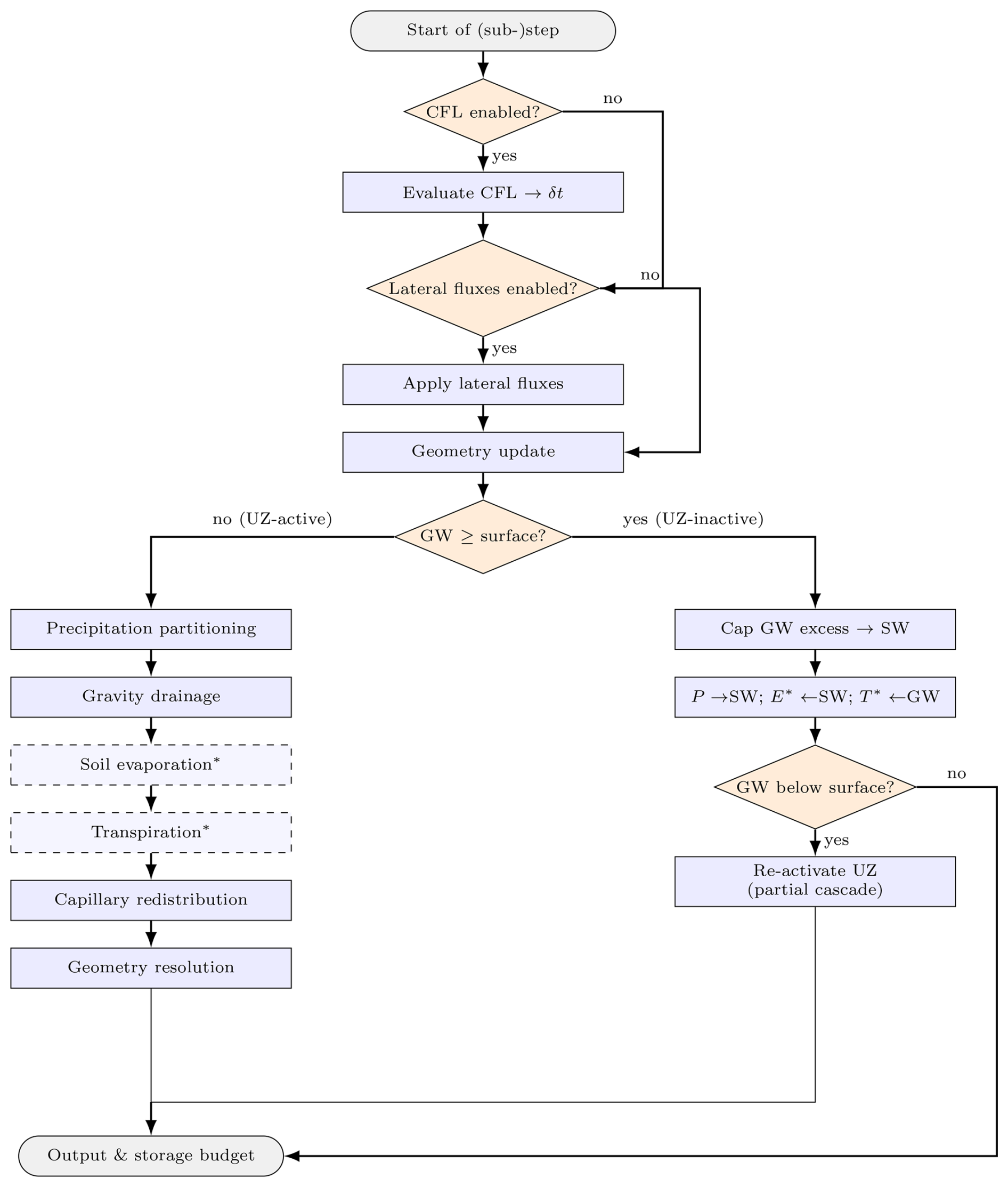
Figure A1 Per-(sub-)step control flow of the explicit operator-split bucket-sequence solver. After CFL adaptive sub-stepping and the optional lateral-flux injection, the saturation gate selects either the UZ-active branch (precipitation partitioning, gravity drainage, optional ET sinks, capillary redistribution, geometry resolution) or the saturated-column branch (top-cap to SW, surface-input rerouting, re-activation gate). Optional modules are dashed; an asterisk marks modules that are skipped when the corresponding forcing channel is disabled.

Lateral fluxes. Any prescribed lateral SW and GW source/sink rates are applied first, before any vertical flux is computed. Lateral fluxes are the coupling channel through which an external SW model and an external GW model communicate with GWSWEX, and are treated as instantaneous source/sink terms acting on the SW and GW storages respectively:

$$\begin{array}{}\text{(A12)}& \begin{array}{rl}& {\text{SW}}_t={\text{SW}}_{t-\mathrm{1}}+{\text{SW}}_{\text{lateral}}\cdot \mathrm{\Delta }t,\\ & {\text{GW}}_t=max(z_{\text{bot}}^{\left[n_l\right]},{\text{GW}}_{t-\mathrm{1}}+{\text{GW}}_{\text{lateral}}\cdot \mathrm{\Delta }t),\end{array}\end{array}$$

where SW_lateral and GW_lateral [L T⁻¹] are the net lateral rates (positive into the column). When this module is disabled, ${\text{SW}}_t={\text{SW}}_{t-\mathrm{1}}$ and ${\text{GW}}_t={\text{GW}}_{t-\mathrm{1}}$.

Geometry update. The GW boundary layer index, the active layer thicknesses, the effective pore volumes and the per-layer hydrostatic-equilibrium storage are recomputed from the current GW_t. The boundary layer is the shallowest layer whose bottom lies at or below the groundwater head,

$$\begin{array}{}\text{(A13)}& l_{\text{GW}}=min(l\in \mathrm{1},\mathrm{\dots },n_l:z_{\text{bot}}^{\left[l\right]}\le {\text{GW}}_t),\end{array}$$

and the active thickness and effective pore volume of each layer follow as

$$\begin{array}{}\text{(A14)}& d_{\mathrm{a}}^{\left[l\right]}=\left\{\begin{array}{ll}{z}_{\text{top}}^{\left[l\right]}-z_{\text{bot}}^{\left[l\right]},& l<l_{\text{GW}},\\ z_{\text{top}}^{\left[l\right]}-{\text{GW}}_t,& l=l_{\text{GW}},\\ \mathrm{0},& l>l_{\text{GW}},\end{array}\right.{\text{ePV}}^{\left[l\right]}=d_{\mathrm{a}}^{\left[l\right]}\cdot {\mathit{\theta }}_{\mathrm{s}}^{\left[l\right]}.\end{array}$$

The hydrostatic-equilibrium storage ${\text{UZ}}_{\text{eq}}^{\left[l\right]}$ is the integral of the van Genuchten retention curve over the active depth of the layer, taken with the GW surface as the zero-potential datum. Letting ${\mathit{\psi }}_{m,\text{top}}^{\left[l\right]}={\text{GW}}_t-z_{\text{top}}^{\left[l\right]}$ and, for l<l_GW, ${\mathit{\psi }}_{m,\text{bot}}^{\left[l\right]}={\text{GW}}_t-z_{\text{bot}}^{\left[l\right]}$ (and ${\mathit{\psi }}_{m,\text{bot}}^{\left[l_{\text{GW}}\right]}=\mathrm{0}$), the equilibrium storage is

$$\begin{array}{}\text{(A15)}& {\text{UZ}}_{\text{eq}}^{\left[l\right]}=\underset{{\mathit{\psi }}_{m,\text{bot}}^{\left[l\right]}}{\overset{{\mathit{\psi }}_{m,\text{top}}^{\left[l\right]}}{\int }}\mathit{\theta }\left({\mathit{\psi }}_m\right)\mathrm{d}{\mathit{\psi }}_m,l\le l_{\text{GW}},\end{array}$$

with θ(ψ_m) given by the van Genuchten retention curve from the previous subsection, and ${\text{UZ}}_{\text{eq}}^{\left[l\right]}=\mathrm{0}$ for l>l_GW. The integral is evaluated by composite trapezoidal quadrature with a user-controlled number of sub-intervals n_trapz. When lateral fluxes are disabled and the previous step's geometry resolution did not change GW_t, this update is exact-equal to the carried-forward geometry and is skipped as an optimisation.

Precipitation partitioning. Existing surface water and incident precipitation are combined as the total water available at the surface,

$$\begin{array}{}\text{(A16)}& P=P_{\text{rate}}\cdot \mathrm{\Delta }t,{\text{SW}}_{\text{avail}}={\text{SW}}_t+P,\end{array}$$

and the infiltration capacity is computed from a Green–Ampt expression (Ampt and Green, 1911; Ma et al., 2023),

$$\begin{array}{}\text{(A17)}& \mathrm{\Delta }\mathit{\theta }={\mathit{\theta }}_{\mathrm{s}}^{\left[\mathrm{1}\right]}-{\mathit{\theta }}_{t-\mathrm{1}}^{\left[\mathrm{1}\right]},f_{\text{cap}}=K_{\text{sat}}^{\left[\mathrm{1}\right]}\left(\mathrm{1}+{\displaystyle \frac{{\mathit{\psi }}_{\mathrm{f}}\mathrm{\Delta }\mathit{\theta }}{F}}\right),\end{array}$$

with ψ_f [L] a calibratable suction-head parameter (approximately $\mathrm{1}/{\mathit{\alpha }}^{\left[\mathrm{1}\right]}$ from the van Genuchten curve), Δθ the saturation deficit of the top layer, and F [L] a cumulative-infiltration tracker maintained across steps as a proxy for the wetting-front depth. The actual infiltration over the step is bounded by the capacity, by the available surface water, and by the column sink capacity,

$$\begin{array}{}\text{(A18)}& {\displaystyle }\begin{array}{rl}\text{infiltration}& =min(f_{\text{cap}}\cdot \mathrm{\Delta }t,{\text{SW}}_{\text{avail}},{\text{ePV}}^{\left[\mathrm{1}\right]}\\ & -{\text{UZ}}_{t-\mathrm{1}}^{\left[\mathrm{1}\right]}+S_{\mathrm{y}}^{\left[\mathrm{1}\right]}\cdot (z_{\text{top}}^{\left[\mathrm{1}\right]}-{\text{GW}}_t)),\end{array}\text{(A19)}& {\displaystyle }{\text{SW}}_t={\text{SW}}_{\text{avail}}-\text{infiltration}.\end{array}$$

The third bound is the total unsaturated-zone storage deficit, the unsaturated pore space in the top layer plus the column-wide GW storage capacity, and ensures that ponded water can infiltrate even when the top-layer pore space is already filled by the capillary fringe. The infiltrated volume enters the gravity-drainage module as the inflow to the top layer.

Gravity drainage. Gravity-driven vertical flow is solved sequentially from the top layer downward. For each active layer $l=\mathrm{1},\mathrm{\dots },l_{\text{GW}}$, the inflow is either the surface infiltration (l=1) or the exfiltration from the layer above. The unsaturated conductivity is initially evaluated at the pre-inflow moisture state through the Mualem–van Genuchten relation,

$$\begin{array}{}\text{(A20)}& \begin{array}{rl}& S_{\mathrm{e}}^{\left[l\right]}={\displaystyle \frac{{\text{UZ}}_{t-\mathrm{1}}^{\left[l\right]}/d_{\mathrm{a}}^{\left[l\right]}-{\mathit{\theta }}_{\mathrm{r}}^{\left[l\right]}}{{\mathit{\theta }}_{\mathrm{s}}^{\left[l\right]}-{\mathit{\theta }}_{\mathrm{r}}^{\left[l\right]}}},\\ & K_{\text{unsat}}^{\left[l\right]}=K_{\text{sat}}^{\left[l\right]}\cdot (S_{\mathrm{e}}^{\left[l\right]}{)}^{\mathit{\lambda }}{\left[\mathrm{1}-(\mathrm{1}-(S_{\mathrm{e}}^{\left[l\right]}{)}^{\mathrm{1}/m^{\left[l\right]}}{)}^{m^{\left[l\right]}}\right]}^{\mathrm{2}}.\end{array}\end{array}$$

If the layer receives nonzero inflow during active surface infiltration, K is re-evaluated at the post-inflow state and the effective conductivity is taken as the arithmetic mean of the two estimates,

$$\begin{array}{}\text{(A21)}& K_{\text{eff}}^{\left[l\right]}=\frac{\mathrm{1}}{\mathrm{2}}(K_{\text{pre}}^{\left[l\right]}+K_{\text{post}}^{\left[l\right]}),{\text{TC}}^{\left[l\right]}=K_{\text{eff}}^{\left[l\right]}\cdot \mathrm{\Delta }t,\end{array}$$

otherwise $K_{\text{eff}}^{\left[l\right]}=K_{\text{pre}}^{\left[l\right]}$. The transfer capacity TC^[l] is the maximum volume per unit area that conductivity alone permits to drain from layer l during the step.

A dynamic inter-layer connectivity ratio ${\text{ICratio}}^{\left[l\right]}\in [{\text{ICratio}}_{\text{min}}^{\left[l\right]},\mathrm{1}]$ modulates the effective drainage rate by tracking the fraction of the layer depth reached by the wetting front. Its underlying state is an infiltration-front tracker IC^[l] that advances or retreats by one transfer capacity per (sub-)step depending on whether the layer is receiving inflow:

$$\begin{array}{}\text{(A22)}& \begin{array}{rl}{\text{IC}}^{\left[l\right]}=& \left\{\begin{array}{ll}min({\text{IC}}^{\left[l\right]}+{\text{TC}}^{\left[l\right]},d_{\mathrm{a}}^{\left[l\right]}),& {\text{inflow}}^{\left[l\right]}>\mathrm{0},\\ max({\text{IC}}^{\left[l\right]}-{\text{TC}}^{\left[l\right]},\mathrm{0}),& \text{otherwise},\end{array}\right.\\ & {\text{ICratio}}^{\left[l\right]}=max({\displaystyle \frac{{\text{IC}}^{\left[l\right]}}{d_{\mathrm{a}}^{\left[l\right]}}},{\text{ICratio}}_{\text{min}}^{\left[l\right]}).\end{array}\end{array}$$

The floor ${\text{ICratio}}_{\text{min}}^{\left[l\right]}$ represents the structural macropore connectivity that persists in the absence of recent wetting and is one of the principal calibration parameters of the explicit solver.

The intermediate UZ state after inflow is ${\text{UZ}}_t^{\left[l\right]}={\text{UZ}}_{t-\mathrm{1}}^{\left[l\right]}+{\text{inflow}}^{\left[l\right]}$. Only the storage above hydrostatic equilibrium is allowed to drain (capillary water is held), and the exfiltration is bounded by the transfer capacity, by the free water above equilibrium, and by the connectivity ratio,

$$\begin{array}{}\text{(A23)}& \begin{array}{rl}{\text{UZ}}_{\text{free}}^{\left[l\right]}& ={\text{UZ}}_t^{\left[l\right]}-{\text{UZ}}_{\text{eq}}^{\left[l\right]},{\text{exfiltration}}^{\left[l\right]}\\ & =min({\text{TC}}^{\left[l\right]},max({\text{UZ}}_{\text{free}}^{\left[l\right]},\mathrm{0}\left)\right)\cdot {\text{ICratio}}^{\left[l\right]}.\end{array}\end{array}$$

The intermediate state of the upper layers is then ${\text{UZ}}_t^{\left[l\right]}-={\text{exfiltration}}^{\left[l\right]}$ for $l=\mathrm{1},\mathrm{\dots },l_{\text{GW}}-\mathrm{1}$, and the exfiltration from the boundary layer recharges GW directly,

$$\begin{array}{}\text{(A24)}& {\text{GW}}_t=V_{\text{GW}}^{-\mathrm{1}}\left(V_{\text{GW}}\right({\text{GW}}_t)+{\text{exfiltration}}^{\left[l_{\text{GW}}\right]}).\end{array}$$

The Green–Ampt cumulative infiltration tracker is updated for the next step,

$$\begin{array}{}\text{(A25)}& F=\left\{\begin{array}{ll}min(F,F_{\text{min}})+\text{infiltration},& {\text{SW}}_{\text{avail}}>\mathrm{0},\\ min(F,F_{\text{min}})-{\text{exfiltration}}^{\left[\mathrm{1}\right]},& \text{otherwise},\end{array}\right.\end{array}$$

where F_min [L] is a small floor that prevents the singularity in f_cap at the start of an event.

Soil evaporation. When evaporation is enabled, the potential demand $E_{\text{pot}}=E_{\text{rate}}\cdot \mathrm{\Delta }t$ is applied first to the surface storage, without stress limitation,

$$\begin{array}{}\text{(A26)}& \begin{array}{rl}& E_{\text{SW}}=min(E_{\text{pot}},{\text{SW}}_t),{\text{SW}}_t-=E_{\text{SW}},\\ & E_{\text{residual}}=E_{\text{pot}}-E_{\text{SW}},\end{array}\end{array}$$

and then to the top UZ layer with a Laio-type stress function (Laio et al., 2001) in the saturation $s^{\left[\mathrm{1}\right]}={\text{UZ}}_t^{\left[\mathrm{1}\right]}/{\text{ePV}}^{\left[\mathrm{1}\right]}$,

$$\begin{array}{}\text{(A27)}& E_{\text{lim}}=\left\{\begin{array}{ll}\mathrm{0},& s^{\left[\mathrm{1}\right]}\le s_{\mathrm{h}},\\ E_{\text{residual}}\cdot {\displaystyle \frac{s^{\left[\mathrm{1}\right]}-s_{\mathrm{h}}}{s_{\mathrm{e}}-s_{\mathrm{h}}}},& s_{\mathrm{h}}<s^{\left[\mathrm{1}\right]}\le s_{\mathrm{e}},\\ E_{\text{residual}},& s^{\left[\mathrm{1}\right]}>s_{\mathrm{e}},\end{array}\right.\end{array}$$

with s_h the hygroscopic-point saturation (below which water is bound too tightly to the matrix to evaporate) and s_e a capillary-continuity threshold (below which liquid continuity from the soil to the surface is disrupted). Both can be estimated from the retention curve as $s_{\mathrm{h}}\approx {\mathit{\theta }}_{\mathrm{r}}^{\left[\mathrm{1}\right]}/{\mathit{\theta }}_{\mathrm{s}}^{\left[\mathrm{1}\right]}$ and $s_{\mathrm{e}}\approx {\text{UZ}}_{\text{eq}}^{\left[\mathrm{1}\right]}/{\text{ePV}}^{\left[\mathrm{1}\right]}$, with user override retained for soils whose retention curve does not adequately represent these thresholds. The actual UZ evaporation is then bounded by the water above residual,

$$\begin{array}{}\text{(A28)}& E_{\text{UZ}}=min(E_{\text{lim}},{\text{UZ}}_t^{\left[\mathrm{1}\right]}-{\mathit{\theta }}_{\mathrm{r}}^{\left[\mathrm{1}\right]}\cdot d_{\mathrm{a}}^{\left[\mathrm{1}\right]}),{\text{UZ}}_t^{\left[\mathrm{1}\right]}-=E_{\text{UZ}},\end{array}$$

and the actual evaporation reported for the step is $E_{\text{act}}=E_{\text{SW}}+E_{\text{UZ}}$.

Transpiration. When transpiration is enabled, the potential demand $T_{\text{pot}}=T_{\text{rate}}\cdot \mathrm{\Delta }t$ is partitioned uniformly across the rooted layers of the element. Each model element carries a binary root mask ${\mathrm{1}}_{\text{root}}^{\left[l\right]}\in \mathit{\{}\mathrm{0},\mathrm{1}\mathit{\}}$, set at initialisation by intersecting the per-vegetation-type rooting depth with the layer geometry, and re-evaluated whenever a dynamic root-growth schedule is supplied. Writing $n_{\text{root}}={\sum }_l{\mathrm{1}}_{\text{root}}^{\left[l\right]}$ for the number of rooted layers, the per-layer demand is $T_{\text{pot}}^{\left[l\right]}=T_{\text{pot}}/n_{\text{root}}$ for each rooted layer l with l≤l_GW. The uniform partition reflects the resolution at which the root system is represented: the model knows the rooting depth but not the within-zone root-density profile, and any non-uniform weighting at that level of detail would be unsupported by the input it carries. Each layer's demand is reduced by a Laio stress function in s^[l],

$$\begin{array}{}\text{(A29)}& T_{\text{lim}}^{\left[l\right]}=\left\{\begin{array}{ll}\mathrm{0},& s^{\left[l\right]}\le s_{\mathrm{w}},\\ T_{\text{pot}}^{\left[l\right]}\cdot {\displaystyle \frac{s^{\left[l\right]}-s_{\mathrm{w}}}{s^{*}-s_{\mathrm{w}}}},& s_{\mathrm{w}}<s^{\left[l\right]}\le s^{*},\\ T_{\text{pot}}^{\left[l\right]},& s^{\left[l\right]}>s^{*},\end{array}\right.\end{array}$$

with s_w the wilting-point saturation and s^* the saturation at incipient stomatal closure. Each layer's actual UZ extraction is bounded by the water above residual,

$$\begin{array}{}\text{(A30)}& T_{\text{UZ}}^{\left[l\right]}=min(T_{\text{lim}}^{\left[l\right]},{\text{UZ}}_t^{\left[l\right]}-{\mathit{\theta }}_{\mathrm{r}}^{\left[l\right]}\cdot d_{\mathrm{a}}^{\left[l\right]}),{\text{UZ}}_t^{\left[l\right]}-=T_{\text{UZ}}^{\left[l\right]}.\end{array}$$

If the root system extends into the saturated zone, the demand from those layers is taken directly from GW and bounded by the available drainable volume,

$$\begin{array}{}\text{(A31)}& \begin{array}{rl}& T_{\text{GW}}=min(\sum _{l=l_{\text{GW}}}^{n_l}{T}_{\text{pot}}^{\left[l\right]},V_{\text{GW}}({\text{GW}}_t\left)\right),\\ & {\text{GW}}_t=V_{\text{GW}}^{-\mathrm{1}}\left(V_{\text{GW}}\right({\text{GW}}_t)-T_{\text{GW}}),\end{array}\end{array}$$

and the actual transpiration is $T_{\text{act}}={\sum }_l{T}_{\text{UZ}}^{\left[l\right]}+T_{\text{GW}}$.

Capillary redistribution. When net surface infiltration in the current (sub-)step is below a small threshold (infiltration<ϵ), the model performs a multi-sweep, conductivity-limited capillary redistribution that relaxes the storage profile toward ${\text{UZ}}_{\text{eq}}^{\left[l\right]}$ and represents capillary rise from the GW into the depleted UZ. The module is gated off during active infiltration to prevent the simultaneous downward percolation and upward capillary pull from producing numerical oscillations.

Each sweep proceeds upward from the boundary layer l_GW to layer 1 and uses Gauss–Seidel ordering: each updated storage is immediately visible to subsequent moves. At the start of each sweep the current capillary deficit of each layer is recomputed,

$$\begin{array}{}\text{(A32)}& {\text{cap\_deficit}}^{\left[l\right]}=max({\text{UZ}}_{\text{eq}}^{\left[l\right]}\cdot {\mathit{\beta }}_{\text{hyst}}-{\text{UZ}}_t^{\left[l\right]},\mathrm{0}),\end{array}$$

with ${\mathit{\beta }}_{\text{hyst}}\in (\mathrm{0},\mathrm{1}]$ a hysteresis damping factor that scales the equilibrium target to account for the difference between the desorption curve (on which UZ_eq is built) and the wetting curve being followed during capillary rise. For the boundary layer the supply comes from GW and is bounded only by the deficit and the available drainable volume,

$$\begin{array}{}\text{(A33)}& {\text{cap\_flux}}^{\left[l_{\text{GW}}\right]}=min({\text{cap\_deficit}}^{\left[l_{\text{GW}}\right]},V_{\text{GW}}({\text{GW}}_t\left)\right),\end{array}$$

with GW_t and ${\text{UZ}}_t^{\left[l_{\text{GW}}\right]}$ updated in place. For each upper layer the donor is the layer immediately below; the donor's conductivity is re-evaluated from its current moisture state, the conductivity-limited transfer capacity is ${\text{TC}}_{\text{cap}}^{[l+\mathrm{1}]}=K_{\text{cap}}^{[l+\mathrm{1}]}\cdot \mathrm{\Delta }t$, and the capillary flux is

$$\begin{array}{}\text{(A34)}& \begin{array}{rl}{\text{cap\_flux}}^{\left[l\right]}=& min({\text{cap\_deficit}}^{\left[l\right]},{\text{TC}}_{\text{cap}}^{[l+\mathrm{1}]},\\ & {\text{UZ}}_t^{[l+\mathrm{1}]}-{\mathit{\theta }}_{\mathrm{r}}^{[l+\mathrm{1}]}\cdot d_{\mathrm{a}}^{[l+\mathrm{1}]}),\end{array}\end{array}$$

with the recipient gaining and the donor losing the same amount. Repeated sweeps allow water to propagate upward through several layers within a single (sub-)step, acting as a Picard-like relaxation of the upward Darcy flow under the frozen geometry.

Geometry resolution. After all flux modules have executed, the geometry is recomputed from the updated GW_t. If the groundwater head has reached or risen above the surface, the above-surface drainable volume is routed to SW and the column is fully saturated,

$$\begin{array}{}\text{(A35)}& \begin{array}{rl}{\text{If GW}}_t\ge z_{\text{top}}^{\left[\mathrm{1}\right]}:& {\text{SW}}_t+=({\text{GW}}_t-z_{\text{top}}^{\left[\mathrm{1}\right]})\cdot S_{\mathrm{y}}^{\left[\mathrm{1}\right]},\\ & {\text{GW}}_t=z_{\text{top}}^{\left[\mathrm{1}\right]},{\text{UZ}}_t^{\left[l\right]}=\mathrm{0}\forall l.\end{array}\end{array}$$

The boundary layer index, the active thicknesses, the effective pore volumes, and the equilibrium storages are recomputed under the procedure of the geometry-update step. Layers newly exposed by a falling groundwater head (i.e. l_GW has increased over the (sub-)step) are initialised at residual moisture,

$$\begin{array}{}\text{(A36)}& {\text{UZ}}_t^{\left[l\right]}={\mathit{\theta }}_{\mathrm{r}}^{\left[l\right]}\cdot d_{\mathrm{a}}^{\left[l\right]},l=l_{\text{GW,prev}}+\mathrm{1},\mathrm{\dots },l_{\text{GW}},\end{array}$$

which is the physically consistent, mass-conservative value: the drainable fraction $S_{\mathrm{y}}^{\left[l\right]}\cdot (z_{\text{top}}^{\left[l\right]}-z_{\text{bot}}^{\left[l\right]})$ has already been removed from GW by the process that drove the drop, and only the irreducible ${\mathit{\theta }}_{\mathrm{r}}^{\left[l\right]}$ remains in the now-exposed pore space. Layers newly submerged by a rising groundwater head (l_GW has decreased) have their drainable contribution returned to GW,

$$\begin{array}{}\text{(A37)}& \begin{array}{rl}& V_{\text{sub}}=\sum _{l=l_{\text{GW}}+\mathrm{1}}^{l_{\text{GW,prev}}}max({\text{UZ}}_t^{\left[l\right]}-{\mathit{\theta }}_{\mathrm{r}}^{\left[l\right]}\cdot \left(z_{\text{top}}^{\left[l\right]}-z_{\text{bot}}^{\left[l\right]}\right),\mathrm{0}),\\ & {\text{GW}}_t=V_{\text{GW}}^{-\mathrm{1}}\left(V_{\text{GW}}\right({\text{GW}}_t)+V_{\text{sub}}),\end{array}\end{array}$$

with their UZ entries cleared to zero. Finally, any over-saturation accumulated by the sequence of flux operations is capped by transferring the excess to GW,

$$\begin{array}{}\text{(A38)}& \begin{array}{rl}{\text{If UZ}}_t^{\left[l\right]}>{\text{ePV}}^{\left[l\right]}:& {\text{GW}}_t+={\displaystyle \frac{{\text{UZ}}_t^{\left[l\right]}-{\text{ePV}}^{\left[l\right]}}{S_{\mathrm{y}}^{\left[l\right]}}},\\ & {\text{UZ}}_t^{\left[l\right]}={\text{ePV}}^{\left[l\right]}.\end{array}\end{array}$$

This safety net catches residual numerical overshoot from sequential flux accumulation and is the only post-hoc mass redistribution in the sequence; all other flux limits are structural and embedded in the per-module formulae through min and max operators.

Output and per-step storage budget. At the end of each macro-step the storage changes are compared with the accumulated boundary fluxes to produce per-step diagnostics: GW recharge $r_{\text{GW}}=\mathrm{\Delta }{V}_{\text{GW}}^{\text{int}}/\mathrm{\Delta }t$ from the internal GW volume change net of any lateral exchange, SW runoff $r_{\text{SW}}=max(\mathrm{\Delta }{\text{SW}}^{\text{int}},\mathrm{0})/\mathrm{\Delta }t$, and a mass-balance residual

$$\begin{array}{}\text{(A39)}& {\mathit{ϵ}}_{\text{MB}}=P-E_{\text{act}}-T_{\text{act}}-\mathrm{\Delta }{V}_{\text{GW}}^{\text{int}}-\mathrm{\Delta }{\text{SW}}^{\text{int}}-\mathrm{\Delta }\text{UZ},\end{array}$$

where ΔUZ includes a residual-saturated-zone correction that returns the θ_r⋅z_sat water held in fully saturated layers (which sits outside both ∑_lUZ^[l] and V_GW) to the storage-change accounting. With the correction in place, the column budget $\text{total}={\sum }_l{\text{UZ}}^{\left[l\right]}+V_{\text{GW}}+\text{SW}+{\sum }_l{\mathit{\theta }}_{\mathrm{r}}^{\left[l\right]}\cdot z_{\text{sat}}^{\left[l\right]}$ closes at every macro-step, and ϵ_MB is at floating-point tolerance away from any cap event.

A3.4 Saturated-column branch

Whenever the column is fully saturated at the start of the step (${\text{GW}}_t\ge z_{\text{top}}^{\left[\mathrm{1}\right]}$ after lateral fluxes), the per-process sequence above cannot execute because all ePV^[l]=0. A reduced branch is taken instead. Any GW volume above the surface is first capped to SW at $S_{\mathrm{y}}^{\left[\mathrm{1}\right]}$. All precipitation is then added to SW directly; evaporation is drawn from SW first and from GW as the residual; transpiration is drawn from GW (bounded by $K_{\text{sat}}^{\left[\mathrm{1}\right]}\cdot \mathrm{\Delta }t$, the maximum extraction rate the surface can sustain), since the roots are submerged. A re-activation gate then checks whether transpiration has lowered the groundwater head below the surface; if so, Phase B's precipitation deposit is reversed (otherwise it would be double-counted), all newly exposed layers are initialised at residual moisture, and a partial sequence (precipitation partitioning, gravity drainage, capillary redistribution, geometry resolution) resumes for the remainder of the (sub-)step.

A4 Implicit solver: mixed-form Richards equation

The implicit solver replaces the operator-split sequence with a single, unconditionally stable solve of the one-dimensional mixed-form Richards equation (Celia et al., 1990),

$$\begin{array}{}\text{(A40)}& C\left(h\right){\displaystyle \frac{\partial h}{\partial t}}={\displaystyle \frac{\partial }{\partial z}}\left[K\left(h\right)\left({\displaystyle \frac{\partial h}{\partial z}}+\mathrm{1}\right)\right]-S(z,t),\end{array}$$

where h is the matric pressure head (negative in the UZ, non-negative below the groundwater head), $C\left(h\right)=\partial \mathit{\theta }/\partial h$ is the specific moisture capacity (the analytic derivative of the VG retention curve), K(h) is the Mualem–van Genuchten conductivity, and S(z,t) is a distributed sink representing soil evaporation and root water uptake. In the saturated zone the unconfined drainable porosity $S_{\mathrm{y}}={\mathit{\theta }}_{\mathrm{s}}-{\mathit{\theta }}_{\mathrm{r}}$ replaces C(h) to regularise the linear system; this is the physically correct groundwater-head storage capacity for unconfined conditions and supersedes earlier formulations that used a small specific storativity for numerical regularisation alone.

A4.1 Spatial and temporal discretisation

Each layer is represented by its centroid $z_{\mathrm{c}}^{\left[l\right]}$; head, water content, conductivity, and capacity are all evaluated at the centroid. The Darcy flux between adjacent centroids l and l+1 uses an upstream (donor-cell) weighting of the per-node conductivities (Forsyth and Kropinski, 1997),

$$\begin{array}{}\text{(A41)}& K_{\mathrm{1}/\mathrm{2}}^{[l+\mathrm{1}/\mathrm{2}]}=\left\{\begin{array}{ll}{K}^{\left[l\right]},& q^{[l+\mathrm{1}/\mathrm{2}]}\ge \mathrm{0}\left(\text{downward flow}\right),\\ K^{[l+\mathrm{1}]},& q^{[l+\mathrm{1}/\mathrm{2}]}<\mathrm{0}\left(\text{upward flow}\right),\end{array}\right.\end{array}$$

where the flow direction is taken from the previous Picard iterate. Upstream weighting is preferred over the more familiar thickness-weighted harmonic mean (Haverkamp and Vauclin, 1979) because the harmonic mean stalls wetting fronts entering a dry layer: when one of the two adjacent conductivities is small, the harmonic mean collapses with it and the interface becomes effectively impermeable, even though the upstream (wet) layer is fully able to deliver water. Donor-cell weighting picks the conductivity of whichever cell is supplying the flux, which is monotone, conservative, and consistent with the physical picture of a wetting front advancing into dry soil. The temporal scheme is fully implicit (backward Euler), so the discretisation is unconditionally A-stable and admits arbitrarily large macro-steps; the only stability constraint is on Picard convergence, not on the time step.

A4.2 Picard linearisation and TDMA

The nonlinearity in K(h) and C(h) is removed by Picard iteration (Picard, 1890). At each iteration k, K^k, C^k and θ^k are evaluated at the current head iterate h^k; the mixed-form linearisation of Celia et al. (1990) then approximates the accumulation term as

$$\begin{array}{}\text{(A42)}& {\displaystyle \frac{{\mathit{\theta }}^{n+\mathrm{1}}-{\mathit{\theta }}^n}{\mathrm{\Delta }t}}\approx {\displaystyle \frac{C^k(h^{k+\mathrm{1}}-h^k)}{\mathrm{\Delta }t}}+{\displaystyle \frac{{\mathit{\theta }}^k-{\mathit{\theta }}^n}{\mathrm{\Delta }t}},\end{array}$$

in which the second term is a mass-balance correction that carries the residual of the previous Picard iterate forward; once the iterate has converged ($h^{k+\mathrm{1}}\to h^k$ and so ${\mathit{\theta }}^{k+\mathrm{1}}\to {\mathit{\theta }}^k$), the accumulation reduces exactly to $({\mathit{\theta }}^{n+\mathrm{1}}-{\mathit{\theta }}^n)/\mathrm{\Delta }t$ regardless of how many Picard iterations were taken. This is what gives the mixed-form formulation its mass-conservation guarantee at the converged iterate, in contrast to the strictly head-based form which can lose mass at coarse step sizes (Celia et al., 1990).

Substituting the upstream-weighted discretisation of the Darcy flux into the mixed-form Richards equation gives, for each interior layer l, a tridiagonal equation

$$\begin{array}{}\text{(A43)}& a^{\left[l\right]}{h}^{k+\mathrm{1},[l-\mathrm{1}]}+b^{\left[l\right]}{h}^{k+\mathrm{1},\left[l\right]}+c^{\left[l\right]}{h}^{k+\mathrm{1},[l+\mathrm{1}]}=d^{\left[l\right]},\end{array}$$

with coefficients

$$\begin{array}{}\text{(A44)}& \begin{array}{rl}& a^{\left[l\right]}={\displaystyle \frac{K_{\mathrm{1}/\mathrm{2}}^{[l-\mathrm{1}/\mathrm{2}]}}{\mathrm{\Delta }{z}^{\left[l\right]}\mathrm{\Delta }{z}_{\text{up}}^{\left[l\right]}}},c^{\left[l\right]}={\displaystyle \frac{K_{\mathrm{1}/\mathrm{2}}^{[l+\mathrm{1}/\mathrm{2}]}}{\mathrm{\Delta }{z}^{\left[l\right]}\mathrm{\Delta }{z}_{\text{dn}}^{\left[l\right]}}},\\ & b^{\left[l\right]}=-\left({\displaystyle \frac{C^{k,\left[l\right]}}{\mathrm{\Delta }t}}+a^{\left[l\right]}+c^{\left[l\right]}\right),\\ & d^{\left[l\right]}=-{\displaystyle \frac{C^{k,\left[l\right]}{h}^{k,\left[l\right]}}{\mathrm{\Delta }t}}+{\displaystyle \frac{{\mathit{\theta }}^{k,\left[l\right]}-{\mathit{\theta }}^{n,\left[l\right]}}{\mathrm{\Delta }t}}\\ & -{\displaystyle \frac{K_{\mathrm{1}/\mathrm{2}}^{[l-\mathrm{1}/\mathrm{2}]}-K_{\mathrm{1}/\mathrm{2}}^{[l+\mathrm{1}/\mathrm{2}]}}{\mathrm{\Delta }{z}^{\left[l\right]}}}+S^{\left[l\right]},\end{array}\end{array}$$

where $\mathrm{\Delta }{z}_{\text{up}}^{\left[l\right]}=z_{\mathrm{c}}^{[l-\mathrm{1}]}-z_{\mathrm{c}}^{\left[l\right]}$ and $\mathrm{\Delta }{z}_{\text{dn}}^{\left[l\right]}=z_{\mathrm{c}}^{\left[l\right]}-z_{\mathrm{c}}^{[l+\mathrm{1}]}$ are the centroid-to-centroid distances above and below layer l, and the constant −1 in the gravity term of the Richards equation produces the inter-layer conductivity difference in d^[l] (downward gravity flow is the difference between the conductivities of the two interfaces bracketing the layer, divided by the layer thickness). The boundary rows are modified to carry the prescribed top and bottom fluxes (or heads) as detailed in the next subsection. The resulting tridiagonal system is solved in 𝒪(n_l) operations per iteration by the Thomas algorithm (Conte and de Boor, 1980).

Iteration is terminated when ${max}_l|h^{k+\mathrm{1},\left[l\right]}-h^{k,\left[l\right]}|<{\mathit{\epsilon }}_{\text{tol}}$, with a user-controlled cap k_max on the number of iterations to guard against pathological forcings. Typical values are ${\mathit{\epsilon }}_{\text{tol}}={\mathrm{10}}^{-\mathrm{6}}$ m and k_max=100; in practice convergence is reached in 3 to 8 iterations under the warm-start strategy described below.

A4.3 Boundary conditions and groundwater-head determination

The top boundary switches dynamically between Neumann (prescribed flux) and Dirichlet (prescribed head) modes within each macro-step. While the surface is unsaturated, the top boundary carries a Neumann flux equal to the net atmospheric forcing plus any re-infiltration from the previous step's surface ponding,

$$\begin{array}{}\text{(A45)}& q_{\text{top}}=P_{\text{rate}}-E_{\text{rate}}+{\displaystyle \frac{{\text{SW}}_n}{\mathrm{\Delta }t}},\end{array}$$

so that ponded water from the previous macro-step can re-infiltrate at the maximum rate the soil can accept. If the Picard iterate would otherwise drive h^[1]>0 (i.e. the surface saturates), the boundary is switched to Dirichlet h^[1]=0 and the iteration is restarted; the actual infiltration I_actual is then recovered from the layer-1 mass balance at convergence. The post-step surface storage and runoff diagnostic follow as

$$\begin{array}{}\text{(A46)}& \begin{array}{rl}& {\text{SW}}_{n+\mathrm{1}}=max(P_{\text{rate}}\cdot \mathrm{\Delta }t+{\text{SW}}_n-I_{\text{actual}},\mathrm{0}),\\ & r_{\text{SW}}=min(P_{\text{rate}},max(P_{\text{rate}}-I_{\text{actual}}/\mathrm{\Delta }t,\mathrm{0}\left)\right),\end{array}\end{array}$$

with the runoff rate clipped to $\mathrm{0}\le r_{\text{SW}}\le P_{\text{rate}}$ so that no precipitation is lost or invented in the boundary diagnostic. The explicit and implicit solvers report runoff on the same convention. The bottom boundary is a no-flux Neumann condition representing an impermeable base.

The groundwater head is not prescribed: it is recovered after each macro step by scanning the converged head profile from the column base upward to find the shallowest layer k^* such that h^[k]≥0 for all $k=k^{*},\mathrm{\dots },n_l$ (i.e. the top of the contiguous saturation propagating up from the base). If $k^{*}=\mathrm{1}$ the entire column is saturated and the groundwater head elevation is set to the top of layer 1; otherwise it is obtained by linear interpolation of h across the unsaturated–saturated interface between the unsaturated centroid $k^{*}-\mathrm{1}$ above and the saturated centroid k^* below,

$$\begin{array}{}\text{(A47)}& {\text{GW}}_{n+\mathrm{1}}=z_{\mathrm{c}}^{\left[k^{*}\right]}+{\displaystyle \frac{h^{\left[k^{*}\right]}}{h^{\left[k^{*}\right]}-h^{[k^{*}-\mathrm{1}]}}}(z_{\mathrm{c}}^{[k^{*}-\mathrm{1}]}-z_{\mathrm{c}}^{\left[k^{*}\right]}).\end{array}$$

The contiguous-from-bottom requirement is essential because the top node can carry h^[1]≥0 either because the table has reached the surface or because the Dirichlet boundary has imposed surface ponding on an otherwise unsaturated column; treating h^[1]≥0 as a unique indicator of full saturation would snap GW to the surface elevation the first time the top layer ponds and would destroy the UZ–GW partition.

A4.4 Evapotranspiration as distributed sinks

In the implicit solver, soil evaporation and transpiration enter the Richards equation as the distributed sink term S(z,t), with evaporation acting on the surface layer and transpiration distributed uniformly across the rooted layers using the same binary root mask ${\mathrm{1}}_{\text{root}}^{\left[l\right]}$ described for the explicit solver. It must be noted that the same Laio-type four-saturation-threshold function used in the explicit solver is evaluated at each Picard iterate against the current head profile, so that the actual sink applied to the linear system is consistent with the head being solved for rather than lagged from the previous macro-step. The two solvers therefore use one and the same constitutive description of root-zone water stress; the difference is purely numerical (per-process reduction of the potential demand in the explicit solver versus per-iterate reduction inside the implicit solve) and the residual difference between the two ET trajectories is itself a useful diagnostic of how strongly the soil-water dynamics deviate from local equilibrium.

A4.5 Warm-start, mass conservation, and step-size choice

The converged head profile of step n is used as the initial Picard iterate for step n+1, which substantially reduces the iteration count when forcing varies smoothly. The mixed-form linearisation is mass-conservative at converged Picard iterates; residual mass-balance errors arise principally from the start-of-step evaluation of boundary fluxes (which freezes the atmospheric and lateral rates over each macro-step rather than re-evaluating them inside the iteration). Because the scheme is unconditionally stable, the macro step is bounded only by the required temporal fidelity of the application and by the user's tolerance for that boundary-flux splitting error; in practice the implicit solver is run at step sizes that are an order of magnitude larger than the explicit-solver sub-steps without loss of accuracy.

Appendix B: Software architecture

The implementation is laid out as four loosely coupled layers, each with a single concern. The intent is that an end user can drive the model entirely from the topmost layer with no Fortran knowledge, and that a developer can extend the model by adding modules within one layer without touching the others. The full module-by-module architecture is documented in the open-source repository accompanying the paper; the user- and developer-facing aspects of the design are described below.

B1 Layered structure

•  

  Layer 1: Model kernel. A modern Fortran 2008/18 module that owns the global model singleton (a derived type aggregating all per-element state, parameter, and accumulator arrays), provides the macro-step entry point, and dispatches per element to either the explicit or implicit solver based on a single integer field set at initialisation. The per-element loop is parallelised with OpenMP; the work-sharing schedule is configurable and the unit of parallelism is the element column, which is the natural granularity given that the per-element solver work (CFL sub-step count under the explicit solver, Picard iteration count under the implicit solver) varies markedly across the domain. The kernel is the only module visible to the f2py wrapper; everything else is internal.

•  

  Layer 2: Physics and process modules. Small, single-concern Fortran modules with a strictly acyclic dependency graph. The shared modules host the constitutive relations (van Genuchten retention, Mualem conductivity, specific moisture capacity C(h)), the geometry computations, and the mass-balance accumulators; the inter-node conductivity used inside the implicit Picard loop follows the upstream donor-cell weighting described in Appendix A. The solver-specific modules implement the operator-split sequence and CFL sub-stepping for the explicit solver, and the Richards assembly, TDMA, Picard iteration, ET sink and groundwater-head location for the implicit solver. Pure and elemental procedures are used wherever possible to enable vectorisation and OpenMP worksharing.

•  

  Layer 3: f2py wrapper. A thin Fortran translation layer that exposes scalar and array arguments which f2py can marshal to and from Python. No derived types cross the boundary. Each setter is dimension-free on the Python side (f2py infers element, layer, and material counts from array shapes) and accepts only the user-supplied parameters: derived quantities such as $m=\mathrm{1}-\mathrm{1}/n$ and $S_{\mathrm{y}}={\mathit{\theta }}_{\mathrm{s}}-{\mathit{\theta }}_{\mathrm{r}}$ are computed inside the kernel and are never user inputs.

•  

  Layer 4: Python user-facing API. A GWSWEXmodel class manages the full lifecycle: configuration construction and validation through Pydantic models, input pre-processing and broadcasting, the macro-step loop, NetCDF I/O, checkpointing, and restart, and post-processing utilities. Configuration is built up incrementally through init_*, add_*, set_* calls and is committed by a single init() call, which validates the cross-references between the spatial, temporal, initial-condition, solver, and parameter components, derives any quantities the kernel needs (such as the binary root mask from the per-vegetation rooting depth), allocates the kernel and pushes the resolved configuration across the f2py boundary. On successful return from init() the underlying Pydantic objects are frozen (further mutation raises AttributeError); a failure inside init() leaves the configuration objects mutable so that the user can correct the offending input and retry without rebuilding the entire model. Defaults for every empirical parameter live exclusively in the Pydantic models; the Fortran kernel declares no defaults of its own and accepts only explicitly supplied values, ensuring that all parameter choices are traceable in Python source. The Python layer carries the user's chosen length and time units along with the model and uses them for input validation, plotting, and output labelling, but does not perform any internal unit conversion; the kernel works in whatever consistent unit system the user supplies.

B2 End-user workflow

The minimal end-user entry point is the demonstration script included in the repository; a complete simulation fits in roughly 50 lines. The pattern is always the same:

(1) construct GWSWEXmodel(name, T, L) with the chosen length and time units; (2) build the spatial domain (init_space, add_material, add_vegetation); (3) build the temporal domain (init_time); (4) set initial conditions (set_initial_conditions); (5) choose the solver and parameters (set_solver(solver=“explicit” | “implicit”, ...), set_model_params(...)); (6) provide the forcing series (set_forcing(precip, pet, ptt, lat_gw, lat_sw)); (7) allocate the kernel (init, which performs all cross-component validation, derives the binary root mask, freezes the configuration and pushes it across the f2py boundary), step it (run for the full sweep, or run_step(t) inside a user loop for fine-grained control), and tear it down (deinit).

State and diagnostics are retrieved through get_state() (per-element GWH, GWV, SW, UZ and θ in user units) and get_mass_balance()/mass_balance_history (per-step accumulators in the same user units). Built-in CF-1.8 NetCDF output is enabled by default and can be disabled by passing write_output=False. Checkpointing is provided through save_checkpoint(filepath) and load_checkpoint(filepath), which round-trip every kernel state field needed to resume a run with arbitrary new forcings under either solver, including (for the implicit solver) the converged head profile required for the Picard warm-start.

The choice of solver is a single keyword argument to set_solver. All other configuration (geometry, materials, vegetation, ICs, forcing, lateral exchange) is solver-agnostic; in particular, any analysis, post-processing, plotting, or coupling utility built against the Python API works identically for both solvers. The solver can also be changed mid-simulation, on an initialised kernel, through a single switch_solver call: storage state and accumulators are preserved across the boundary, and the kernel internally translates between the implicit head profile and the explicit unsaturated-storage convention so that the destination solver resumes from the same physical state. This in-place switching mechanism makes per-cell or per-phase solver assignment in a coupled regional model possible without tearing down and rebuilding the kernel; the alternative full-reconfigure path (deinit() followed by a new init() with the alternative set_solver call) remains available for cases that require a different domain or set of materials alongside the solver change.

B3 Extension points

The layered structure places the typical extension entry points predictably:

Adding a new soil constitutive law (e.g. an alternative retention curve): add a pure function to the shared physics module, add a selector field and the corresponding parameter group to the Pydantic configuration, and dispatch on the selector inside the constitutive evaluation calls in the relevant solver module(s). No other module changes are required.

Adding a new ET stress function (e.g. Feddes et al., 1978 alongside Laio et al., 2001): add the function to the shared physics module, add a stress_model selector to the corresponding Pydantic parameter model, and dispatch on the selector inside the explicit-solver evaporation/transpiration routines and the implicit-solver ET-sink routine.

Adding a new flux module to the explicit sequence (e.g. preferential flow, snowmelt routing): create a new Fortran module under the explicit-solver directory, expose any new state through the shared types module and the f2py wrapper, insert a single call at the appropriate point in the explicit solver driver, and add a Pydantic model and Python set_* method for the new parameters. The CFL evaluator should be extended with any new stability constraint the new module introduces.

Extending the implicit solver (e.g. an alternative inter-node conductivity weighting, a different Picard relaxation strategy, or an additional sink term in the Richards assembly): modify the relevant pure procedure inside the implicit-solver module (constitutive evaluation, TDMA assembly, or sink injection), expose any new control parameter through the shared types module, the f2py wrapper, and the corresponding Pydantic model, and update the warm-start logic only if the new feature changes the shape of the carry-over head profile. The Picard outer loop, the convergence test $\Vert \mathit{\delta }h{\Vert }_{\mathrm{\infty }}<{\mathit{\epsilon }}_{\text{tol}}$, and the post-step groundwater-head recovery routine are insulated from these changes.

External coupling (e.g. to an external SW model and an external GW model that exchange fluxes with GWSWEX at different intervals): use set_lateral(gw, sw) immediately before each run_step(t) to inject the externally computed lateral rates, and read GWSWEX's reciprocal accumulators (acc_recharge, acc_runoff, acc_lat_gw, acc_lat_sw) from get_mass_balance() after each step. The Python layer treats lateral fluxes purely as configurable per-step inputs, so the coupling protocol, whether explicit, iterative, or operator-split, is decided by the driving framework rather than by GWSWEX itself.

B4 Build and reproducibility

The build system is Meson with meson-python for PEP-517 wheels and f2py for the Fortran–Python bridge. The compilation order is set by the acyclic module dependency graph: shared modules first (constants, types, physics, geometry, mass balance), then the explicit-solver and implicit-solver modules in either order, then the kernel, all linked into a static library; f2py then compiles the wrapper against that library to produce the Python extension module imported by the user-facing API. Both solvers are linked into the same artefact and dispatched at run time, so unused code paths incur no runtime cost. The OpenMP element loop is the only source of parallelism inside the kernel; the thread count is controlled either by the standard OMP_NUM_THREADS environment variable, by passing omp_threads=N to set_solver, or by GWSWEXmodel.set_omp_threads(N) at any point in the model lifecycle (the call routes through to omp_set_num_threads after init, and is recorded in the solver configuration before it). The accompanying pytest suite exercises both solvers end-to-end and includes regression tests for the long-run per-step storage budget.