Modelling wind farm effects in HARMONIE-AROME (cycle 43.2.2) – Part 2: wind turbine database and application to Europe

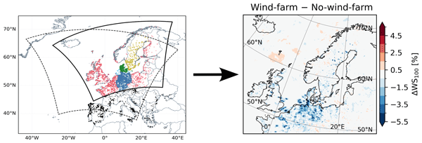
Wind farm parameterizations (WFPs) are used to include the effects of operating wind farms on near-surface weather variables simulated by weather forecasting. In the first part of this series of papers, we implemented and evaluated two WPFs in the HARMONIE-AROME numerical weather prediction model (Fischereit et al., 2024). In this second part, we apply them in HARMONIE-AROME to perform sequential weather forecasts for Northern Europe with a lead time of 48 h every 12 h for two separate months. Combined, the selected summer and winter months are shown to represent the 30-year wind climate (wind speed, wind direction, and stability) in the forecast area reasonably well.

A European wind turbine database is constructed as an input for the forecasts by combining eight different sources, harmonizing and filling gaps in the combined data set, filling missing data using random forest-based models, and associating wind farm information with individual turbines using a developed wind farm splitting algorithm. The final product and the algorithms are published for open access.

We included scenarios for the forecasts with both on- and offshore turbines, as well as only offshore turbines, and analyzed the impact of wind farms on the hub height wind and near-surface temperature forecast. The forecasts using the WFPs show strong reductions in hub height wind speed near the wind farms. Wind forecast using the WFP of Fitch et al. (2012) compares best with observations for all sites, especially for mast and lidar sites close to wind farms. Onshore turbines have a non-negligible wake effect both in terms of strength and area, and must, therefore, be included for accurate wind forecasting. The differences in wind speed between forecasts ignoring wind farms and with a WFP included are statistically significant for many on- and offshore farms. The impact of wind farms on near-surface temperature is small on average over the 2 months, but can be considerable during certain periods. The two WFPs cause opposing signs of impact, i.e., warming versus cooling during nighttime.

1 Introduction

The increasing size and number of wind farms in some places on Earth has been demonstrated to impact many aspects of the lower atmosphere weather. This includes effects on hub height wind (Cañadillas et al., 2020; Platis et al., 2020), 10-m wind (Christiansen and Hasager, 2005), temperature and humidity (Platis et al., 2020, 2023) and ocean waves (Larsén et al., 2024), indicating that to be more accurate, weather forecasts must consider the effects of wind farms on the atmosphere. To do so, several numerical weather prediction (NWP) models now include wind farm parameterizations (WFPs) (Fischereit et al., 2022a).

In this study, we use the NWP model HARMONIE-AROME (abbreviated HARMONIE in the following), which is used by at least 11 national weather services in Europe. In previous studies by van Stratum et al. (2022) and Fischereit et al. (2024), two wind farm parameterizations were implemented in HARMONIE: the wind farm parameterization developed by Fitch et al. (2012) and the Explicit Wake Parameterization (EWP) developed by Volker et al. (2015). In Fischereit et al. (2024), the first part of this series of articles, the two WFPs were compared and preliminarily validated against flight measurements and Weather Research and Forecasting (WRF) model simulations. They showed reasonable good performance compared to observations in selected case studies. Many studies have compared the EWP and the WFP by Fitch et al. (2012) (e.g. Pryor et al., 2020; Larsén and Fischereit, 2021; Ali et al., 2023; Fischereit et al., 2024); however, only a few have compared the results for longer simulations and against measurements. In this paper, longer forecasts are made with the goal of assessing the impact of the WFPs on weather forecasts with both WFPs.

Although there have been many studies using WFPs implemented in the WRF model (see the review by Fischereit et al., 2022a), only very few studies have used them in HARMONIE (van Stratum et al., 2022; Fischereit et al., 2024; Dirksen et al., 2022) or other operational NWP models. Out of those few, van Stratum et al. (2022) and Dirksen et al. (2022) have used HARMONIE in hindcast mode, i.e., using reanalysis data as initial and boundary conditions and not assimilating any observations. In this study, we use extensive data assimilation and global forecasting data as boundary conditions, combined with the last forecast as initial conditions (warm start) to ensure realistic NWP forecasting conditions, in a setup similar to the operational NWP forecasts at the Danish Meteorological Institute (DMI).

NWP forecasts are used for power forecasts, making it important to investigate the wind farm wake effects on wind speed. In addition to this focus, we also focus on temperature at 2 m height, since this is an important parameter for the public. Wind turbines and wind farms have been shown to affect near-surface temperature. In particular, during stable conditions, often at nighttime, a warming of the land surface temperatures (Xia et al., 2019) and near-surface temperature (Wu and Archer, 2021) as well as at hub height (Platis et al., 2020) has been found from measurements and modelling. However, the mechanism for the warming is not yet fully understood, due to the lack of appropriate measurements. Some studies attribute the warming to the enhanced mixing reaching the surface (Platis et al., 2020), while Wu and Archer (2021) found from measurements in the wake of a single turbine over land that the increased mixing does not reach the surface and is instead only enhanced above hub-height due to increased shear and blade-induced turbulence. Instead, they proposed that a near-surface warming was the result of a convergence of downward heat fluxes in stable conditions with or without ground-based inversion. However, the enhanced mixing above hub-height drives this convergence. Xia et al. (2019) also found in their modelling study with the WFP by Fitch et al. (2012) in WRF that vertical divergence of heat fluxes is an important mechanism but also 3-dimensional temperature advection. Furthermore, Xia et al. (2019) found that surface heat fluxes were changed, while Wu and Archer (2021) did not find that in their measurements for a single turbine. However, they also argue that the impact of multiple turbines might be different from that of a single turbine due to overlapping wakes. Thus, while the mechanism is not yet fully understood, it seems clear that stability, and particularly in lower rotor lapse rate (Wu and Archer, 2021), is an important determinant of temperature changes near the ground, with stable conditions leading to warming. Furthermore, the location of an inversion (near-surface, below rotor, at hub-height) seems to be a controlling factor (Platis et al., 2018; Wu and Archer, 2021) as well as the wind speed itself (Quint et al., 2025). Furthermore, the turbine size seems to play a role: for higher turbines, the impacts remain aloft (Golbazi et al., 2022). We will investigate how these wind farm-induced near-surface temperature changes manifest in HARMONIE.

All WFPs require the location and characteristics, such as hub height, rotor diameter, thrust, and power curves, of wind turbines whose effect is to be simulated. However, to our knowledge, no database of that type exists yet for Europe. Therefore, the second goal of this manuscript is to present a method to generate a European wind turbine database (WTD). Having this comprehensive WTD at hand allows not only to compare the results of the two parameterizations, but also to compare the impact of including onshore wind farms, which has not been done in previous studies. Compared to offshore turbines, the impact of onshore turbines is expected to be smaller, due to higher background turbulence levels. However, long wind farm wakes longer than 50 km have also been simulated onshore in the United States (Lundquist et al., 2019). In this study, we will investigate whether the inclusion of onshore turbines alters the forecasted fields, which may indicate that these should not be ignored for a more accurate NWP.

The manuscript is structured as follows: Sect. 2 describes the new wind turbine database. Section 3 describes the model setup of HARMONIE for the simulations using the WTD. In Sect. 4, the forecasts are evaluated against measurements, and in Sect. 5, the wind farm impacts both on wind speed and on temperature are analyzed. In Sect. 6 we discuss the results and conclude in Sect. 7. In the appendices, additional information on the retrieval and processing of some of the data for the WTD is given (Sect. A1 for OpenStreetMap and Sect. A2 for Emodnet). In Sect. A3 the representativeness of the selected simulation period is discussed. Additional simulation results, such as monthly averages of wind speed and daytime temperature, are presented in Sects. A4 and A6. Finally, the methodology of the applied significance test for spatially and temporally autocorrelated data is described in Sect. A5.

2 A European wind turbine database

The geographic location and the turbine characteristics (especially hub height, rotor diameter, and thrust coefficient) are required to represent the impact of wind turbines and wind farms on atmospheric flow. In recent years, significant efforts have been made to create freely available regional or global databases of wind turbine locations and characteristics (e.g. Open Power System Data, 2020; Dunnett et al., 2020; Zhang et al., 2021; Hoeser and Kuenzer, 2022) or as part of commercial products (e.g. The Wind Power, 2021). However, to our knowledge, there is no single source that combines sufficient information about wind turbine locations and detailed turbine specifications (including geometric properties as well as thrust and power curves) on turbine level over the whole of Europe, including on- and offshore areas. This lack of data makes it difficult to accurately include turbine effects in operational NWP. In addition, for operational NWP this information should be kept up-to-date.

To overcome these challenges, various data sources (both for wind turbine characteristics and location information) were post-processed and combined to create a homogenized European wind turbine dataset for NWP models. Along with the derived database, we publish the algorithm to create the database (Imberger et al., 2025) so it is possible to update it. In Sect. 2.1, the different data sources are summarized, and the wind farm splitting algorithms (WFSA) are introduced that make use of wind farm aggregated turbine information and openly available turbine location data from OpenStreetMap (OSM) to derive turbine-level information. In Sect. 2.2, we summarize how to obtain the turbine characteristics, which includes a statistical regression model based on the Random forests method (Ho, 1995) to fill in missing values in the turbine specification information.

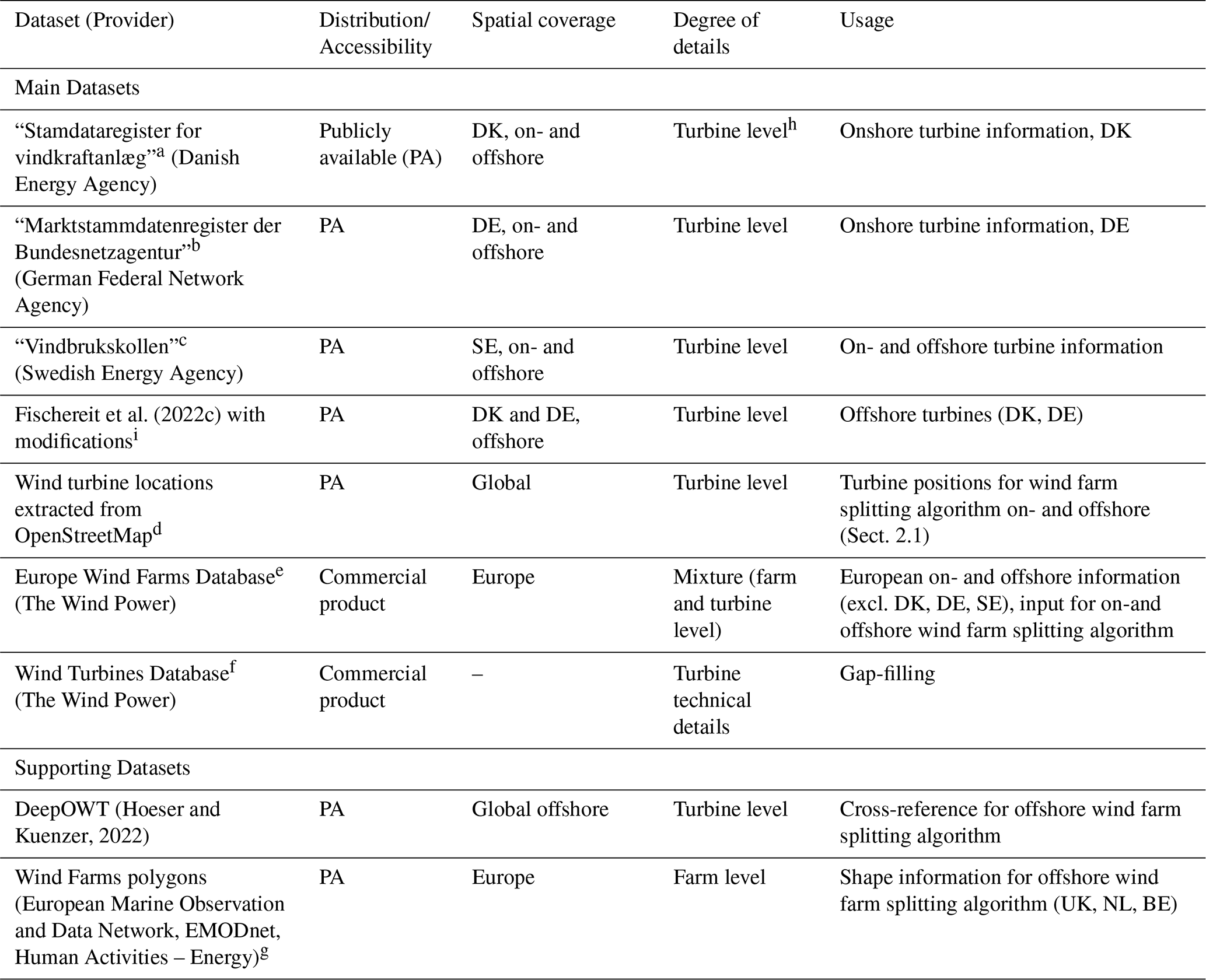
Fischereit et al. (2022c)Hoeser and Kuenzer, 2022

Table 1 Data sources used for deriving the European wind turbine dataset. DK: Denmark, DE: Germany, SE: Sweden, UK: United Kingdom, BE: Belgium, NL: The Netherlands. PA: Publicly Available.

^a https://ens.dk/service/statistik-data-noegletal-og-kort/data-oversigt-over-energisektoren (last access: 20 October 2021)
^b https://www.marktstammdatenregister.de/MaStR/Einheit/Einheiten/OeffentlicheEinheitenuebersicht (last access: 19 October 2021)
^c https://vbk.lansstyrelsen.se/en (last access:: 24 March 2022)
^d https://www.openstreetmap.org, last access: 1 October 2022 using query described in Appendix A1
^e https://www.thewindpower.net/store_continent_en.php?id_zone=1001, last access: 1 October 2021, European subset of global data product purchased in October 2021
^f https://www.thewindpower.net/store_manufacturer_turbine_en.php?id_type=4, last access: 1 October 2021, Turbine technical database product purchased in October 2021
^g https://emodnet.ec.europa.eu/geoviewer/ (last access: 24 March 2022)
^h Only installed capacities larger than 6 kW.
ⁱ Dutch Gemini I and II farms removed, Baltic Sea wind farms Wikinger (DE), Arkona (DE), Baltic 1 and 2 (DE), Rødsand (DK), Nysted (DK), Kriegers Flak (DK), Anholt (DK), Middelgrunden (DK) as well as Rønland (DK) and Nissum Bredning (DK), Danish Limfjord (DK), added. Available as tabulated data in (Imberger et al., 2025)

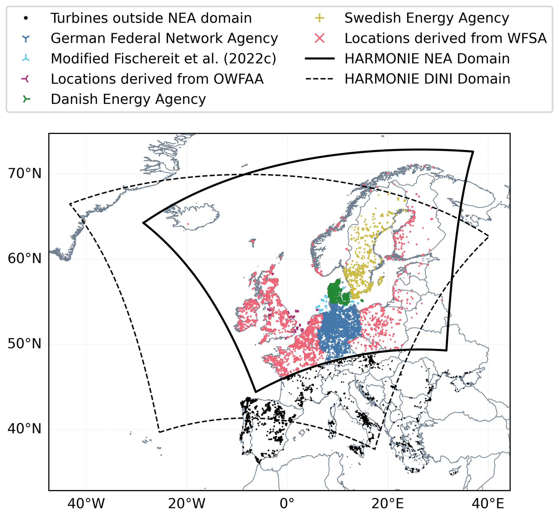
Figure 1 Wind turbine locations after post-processing and combining the different data sources listed in Table 1 within the different operational HARMONIE domains at Danish Meteorological Institute (DMI, black lines). The domain with a solid outline is the Northern Europe DMI domain A (NEA), mainly used in this study. Dashed outline is the Denmark-Ireland-Netherlands-Iceland (DINI) domain used for the sensitivity test in Sect. 5.4. Modified Fischereit et al. (2022c) refers to the dataset presented in that publication with modifications (cf. Table 1). Turbines available in the WTD, but located outside the NEA domain, are displayed as black dots.

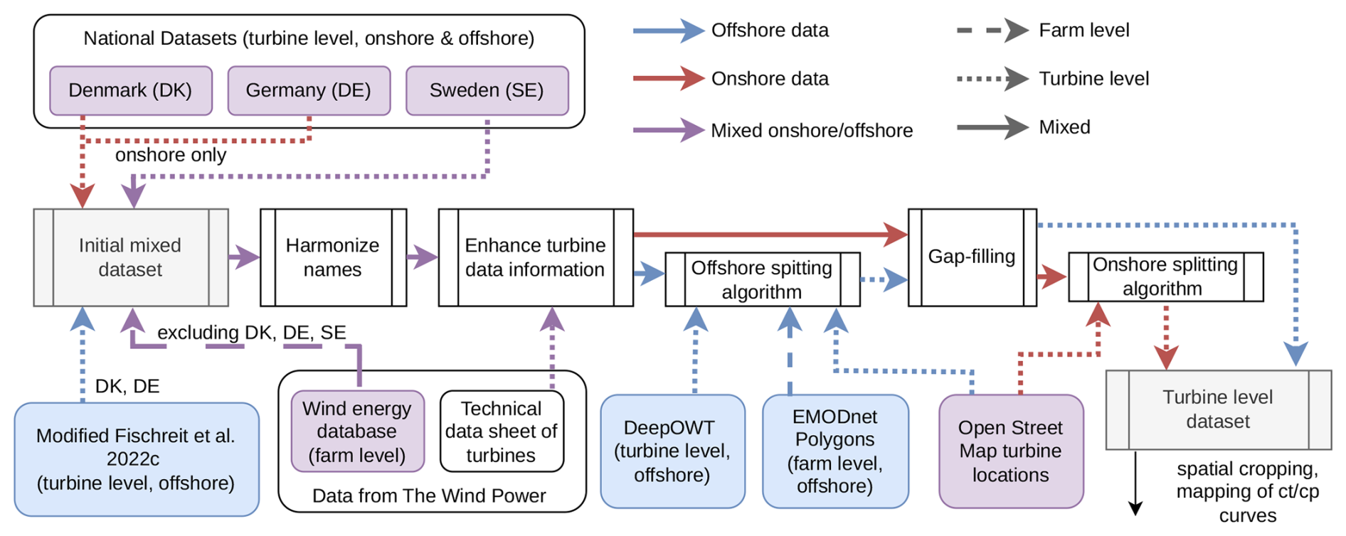
Figure 2 Illustration of the workflow behind the wind farm database connecting the different input sources in Table 1 to the final merged, gap-filled, turbine-level wind farm dataset.

2.1 Wind turbine locations

Depending on the country and region, information about wind turbine locations is obtained from different data sources (Fig. 1). An overview of all main and supporting datasets is provided in Table 1, while Fig. 2 illustrates their connection to the database generation workflow. For onshore locations in Denmark, Germany, and Sweden, input from the national datasets from the Danish Energy Agency, German Federal Network Agency, and Swedish Energy Agency is used, respectively. Tailored data cleaning and processing steps (among others, spatial filtering, treatment of commissioning/decommissioning of turbines, removal of obvious nonphysical values, omitting corrupted data locations, etc.) are required due to the different reporting strategies of the different agencies. For details, the reader is referred to the repository of the wind turbine database creation algorithm (Imberger et al., 2025).

The modified dataset from Fischereit et al. (2022c) is used for offshore wind turbine locations around Denmark because it underwent additional manual checks. The national and custom datasets already provide turbine locations and specifications at the turbine level. Outside the regions mentioned above, wind turbine specifications are obtained from the European Wind Farms Database (EWFD). However, this database mostly offers wind farm-level information, such as aggregated installed capacity, number of turbines per farm, and the latitude/longitude of the wind farm, rather than details for individual turbines. This can be problematic, especially for very large wind farms in terms of area and capacity, because the entire wind farm could be mapped to a single grid cell in the NWP model, potentially causing unrealistic spikes and numerical instabilities. To address this, two wind farm splitting algorithms were developed here, one for onshore locations (WFSA) and one for offshore locations (OWFSA).

For onshore wind farms, wind farm shape information is rarely available, and thus, a more generic splitting algorithm is applied. Starting from the wind farm locations in the EWFD, the WFSA searches radially for the nearest wind turbine locations in the OSM database until the number of turbines specified in the EWFD is reached. The central wind farm coordinate is then replaced by the corresponding turbine locations. If the algorithm does not converge (that is, fewer than the reported number of turbines found within an 85 km radius in the OSM database), only the found turbines are included in the dataset. Turbine specifications from the EWFD associated with the wind farm are propagated to all individual turbine positions. While it is expected that the splitting in highly dense wind farm clusters or very stretched and irregular wind farms will have challenges, the large amount of wind farm locations in the EWFD (more than 3500 listed wind farms) makes it difficult to design universally applicable algorithms with an in-depth quality check of all cases. This will add different degrees of uncertainty to the WFSA-derived turbine locations (see also Discussion in Sect. 6).

For offshore wind farms, on the other hand, wind farm shape and layout information is more commonly available (mostly in the form of geospatial shapefiles). For our workflow for the OWFSA, we make use of wind farm layout information from the European Marine Observation and Data Network (EMODnet) Human Activities – Energy (see details in Table 1 and Appendix A2 for a depiction of the raw data) to more accurately map the farm-level information from EWFD to individual turbines provided by OSM. It must be noted that some polygons in EMODnet were merged based on visual inspection to increase alignment with EWFD information (cf. Appendix A2). During the development of the database, small inaccuracies in the reporting of the turbine locations can discard otherwise valid turbines because they just fall outside the borders of the EMODnet polygons. To circumvent this, we follow an iterative approach over different buffer zones (0, 0.00025, 0.0005, 0.0014, and 0.0025°). The steps and magnitudes were calibrated based on wind farms in the Belgian–Dutch offshore area, where the wind farms are placed very close to each other. While derived in the Belgian offshore region, those buffers are applied to all polygons in the EMODnet dataset. During each iteration, the number of OSM turbines is compared to the number of turbines expected by EMODnet and declared as a match if within a tolerance of three turbines (to cope with occasionally misreported turbines in OSM or the number of turbine information in the EWFD and EMODnet database). EWFD farm-level information is then mapped to all identified turbines. If no match has been found, the polygon buffer is increased, and the check is repeated. For EWFD farm-level data that is still without a match, we consult a second turbine-level dataset that is only available offshore (DeepOWT, deep learning derived global offshore wind turbines, Hoeser and Kuenzer (2022), cf. Table 1) and repeat the algorithm for the list of buffer zones. As the final step, we perform a last iteration with the OSM data, but with a polygon buffer of 0.02° to address cases where the farm-level center point information has been reported with insufficient accuracy in the EWFD. Farm-level information that still remains unmapped indicates a too large information mismatch in terms of the reported number of turbines or location information among the three products (OSM, EWFD, EMODnet) and thus has been dropped from the dataset. This happens in a couple of wind farms (13 out of 62 offshore farms) in Finland, the UK, Ireland, the Netherlands, and Norway. However, relative to the total installed capacity associated with the 62 farms, this equates to less than 5 % (if we use the Wind Power data as a reference), thus, it affects mostly smaller farms either in terms of rated power per turbine or number of turbines. Due to the generic nature of the algorithm, this is an acceptable deviation. In total, the developed wind turbine database includes more than 84 000 turbines.

After all wind farm information has been processed (including the mapping of turbine characteristics, see Sect. 2.2), a spatial filter has been applied based on the outlines of HARMONIE's domain (Northern Europe DMI domain A (NEA) or Denmark-Ireland-Netherlands-Iceland (DINI), including a buffer of 0.2°, to the border, see Fig. 1 for the spatial extent of the domain) to only include turbine information within the simulation domain. After applying the spatial filter, around 59 000 turbines are left in the NEA domain, and more than 75 000 in the DINI domain.

2.2 Turbine characteristics

Creating a homogeneous dataset of turbine characteristics presents several challenges. The first is heterogeneous data formatting. To deal with this, we harmonized the manufacturer and turbine model names via automatic and manual filtering and conversion to fixed naming conventions. The second involved suspicious and unrealistic values. We implemented filters to exclude such data points from the final dataset. The third, and perhaps the most challenging, is data gaps. Here, the datasets have missing or incomplete information about the turbines (some of these arise from the second challenge above). To deal with this challenge, we gap-filled these variables. First, by looking up the variables in a technical table (“Wind Turbines Database” in Table 1) with information about many turbine models using the harmonized turbine model names, we performed the look-up. Secondly, we gap-filled the continuous variables by fitting regression models using the Random Forest method. The following sub-section shows the results when applied to turbines in the NEA domain.

2.2.1 Harmonization of names

The harmonization of manufacturer names involved fixing and unifying capitalization and combining names for manufacturers that have merged. We unified the turbine model names by selecting the most frequently used format for that manufacturer. For example, the strings “V126-3.6 MW” and “V126-3600” are both converted to the chosen standard format for Vestas “V126/3600”. Although further harmonization is possible, the harmonization already resulted in a reduction of unique manufacturer values from 198 to 127 and unique turbine models from 3871 to 1278.

2.2.2 Filtering the data

A set of filters was created to detect and remove unrealistic values from the dataset. These filters were used for rated power, P_rated, rotor diameter, D, hub height, H, and the commissioning year, Y.

• P_rated and D were removed (set to NaN) when P_rated < 10 kW and when the ratio $r=P_{\text{rated}}/\left(\mathrm{1000}{D}^{\mathrm{2}}\right)$ is outside the range [0.1,1.0].

• The turbine model, H and D were removed for unrealistically large H or D for older Y, physically impossible hub-height to diameter ratios, and very small rotors and hub heights:

  • $Y<\mathrm{1980}\wedge H$ > 40 m

  • $Y<\mathrm{1980}\wedge D$ > 30 m

  • $Y<\mathrm{2000}\wedge H$ > 140 m

  • $Y<\mathrm{2000}\wedge D$ > 100 m

  • H < 15 m

  • D < 12.5 m

  • $H/D$ < 0.5

2.2.3 Missing data

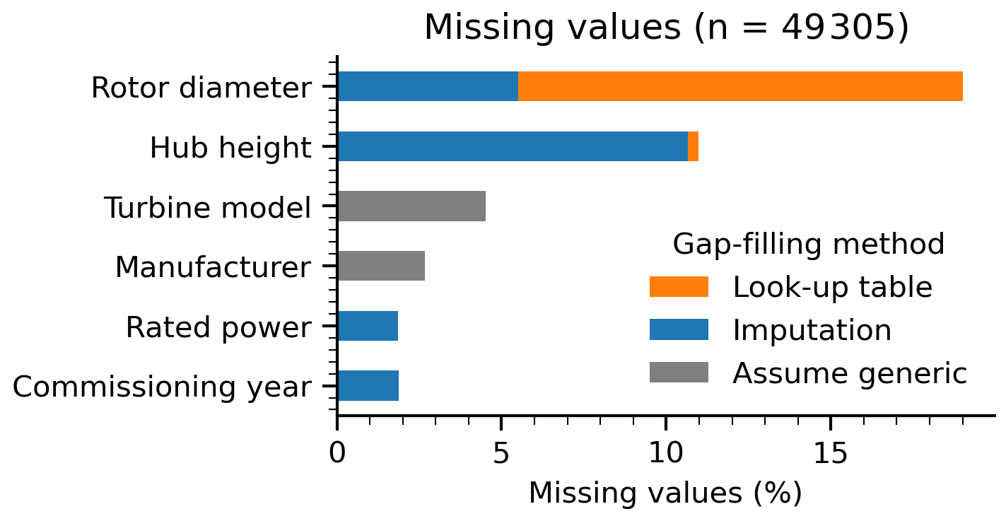
Out of the about 84 000 wind turbines in the full database, each with its 6 defining variables (rotor diameter, hub height, turbine model, manufacturer, rated power and commissioning year), about 49 000 turbines are missing at least one of the 6 variables and many are missing more than one, including preexisting missing values and data removed during filtering. Figure 3 shows the proportion of these missing values in the database spatially filtered to the NEA domain (Sect. 2.1). The figure also shows what proportion of the missing values were filled by a look-up-table, imputed via statistical modeling and assumed generic. The rotor diameters and hub heights are the most frequently missing information. However, while we were able to fill most rotor diameters by look-up, hub heights generally had to be imputed. We do not attempt to gap-fill the missing manufacturer and turbine model data. Instead, missing values for these two variables are assigned to new generic classes, described further in Sect. 2.2.7.

Figure 3 Proportion of missing values in the full European wind turbine database.

2.2.4 Gap-filling via look-up tables

The turbine technical database (The Wind Power, 2021) was used to look up missing rotor diameters and hub heights using the harmonized turbine model names. While a single rotor diameter is associated with each turbine model, the database lists both a minimum and maximum hub height, which can have a large spread. As the final hub height, we used the average of the minimum and maximum hub height, but only when they differed by 9 m or less. This was a somewhat arbitrary choice based on the assumption that the imputation by regression would be better in case a larger discrepancy between the minimum and maximum was present in the database.

2.2.5 Imputation via regression models

To gap-fill the remaining missing values for the rotor diameter, hub height, rated power, and commissioning year, a series of four regression models was trained on the gap-free data, one model for each of the four variables. The four variables were used both as target variables and explanatory variables, adding three more variables only used as explanatory: longitude, latitude, and country. We chose to include these extra variables with the assumption that regional differences may exist in the sizes of turbines, which the regression models could capture. The correlation between these seven variables is shown in Fig. 4. Rated power is, for obvious reasons, strongly correlated with the rotor diameter, but strong correlations are, in general, present between all four variables to be imputed. The variables associated with spatial information are not strongly correlated, except for a weak correlation with each other.

Figure 4 Correlation matrix between the various variables used for the gap-filling models.

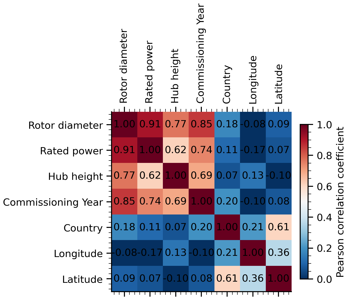
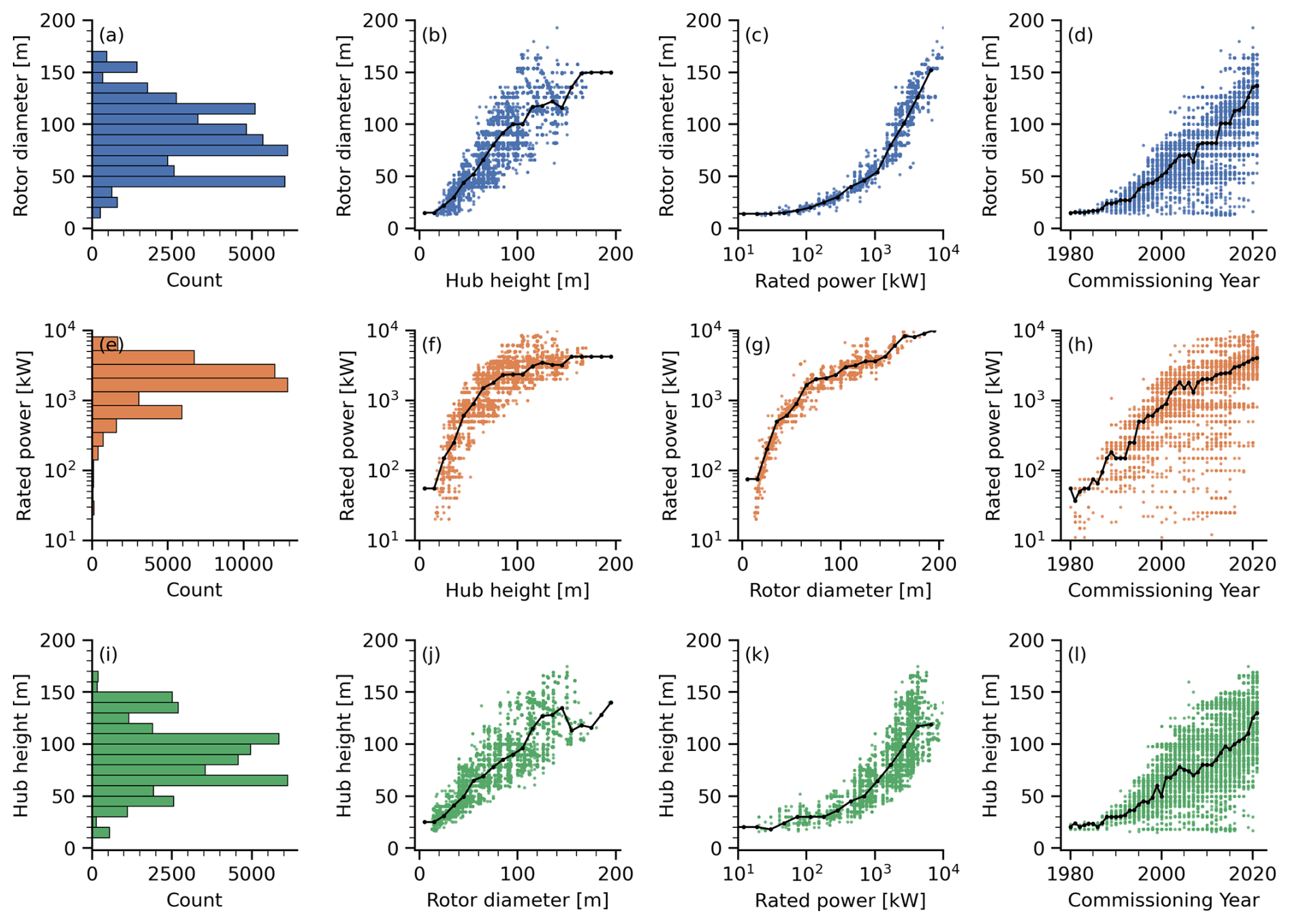
Figure 5 Rotor diameter, rated power and hub height distributions and relationships in the turbine dataset. Top, middle, and bottom rows represent each variable. First column (plots a, e, and i) displays histograms; Middle plots (b, c, f, g, j, and k) illustrate co-variation between variables: rotor diameter with hub height and rated power; rated power with hub height and rotor diameter; and hub height with rotor diameter and rated power. Last column (plots d, h, and l) show variation over commissioning year. Black lines indicate median values within variable bins.

Figure 5 shows the distributions of the rotor diameter, rated power, and hub height, as well as their relationships with the other variables. The evolution of the commissioning year shows, for instance, the growth in turbine size over time.

We sequentially filled data gaps, starting with rated power, followed by rotor diameter, hub height, and commissioning year. For each variable, a random forest regression model was trained in Python (Scikit-Learn v1.5.2) using default parameters. The remaining six variables served as explanatory features, with missing predictors temporarily imputed using binned medians of another variable. These binned medians, shown as black dots and lines in Fig. 5, were applied sequentially, prioritizing hub height, rotor diameter, rated power, and commissioning year as needed.

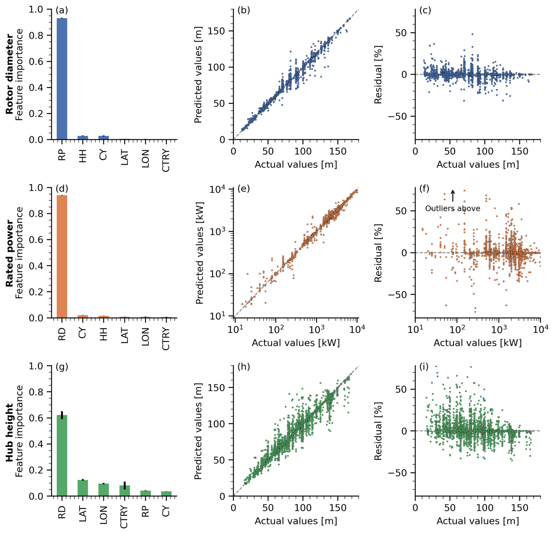
Figure 6 Feature importance and model evaluation for gap-filling models of rotor diameter, rated power, and hub height. (a, d, and g): Feature importance of explanatory variables – rotor diameter (RD), hub height (HH), rated power (RP), commissioning year (CY), country (CTRY), latitude, and longitude (LAT and LON). Bars represent the mean and standard deviation of feature importance estimated by MDI across 100 random forest estimators. (b, e, and h): Scatter plots of actual versus predicted values. (c, f, and i): Model residuals (errors) in percent relative to actual values.

After removing two samples with all relevant variables missing, the dataset contained 49 303 turbines. We trained the regression models on 80 % of the full dataset and used them to impute the missing values. The mean decrease in impurity ((MDI) Breiman et al., 2017) was used to assess the feature importance in these final models. Figure 6 shows, for rotor diameter, rated power, and hub height, the feature importance for the explanatory variables and plots of the scatter and residuals between the model predictions and the actual values for the 20 % held-out samples together with mean scores from the five-fold cross-validation.

Table 2 Cross-validation results for four gap-filling regression models, showing mean evaluation metrics: r², RMSE, MAE, and MAPE—based on a five-fold split of 2937 samples from the gap-free dataset, selected to minimize overfitting and bias.

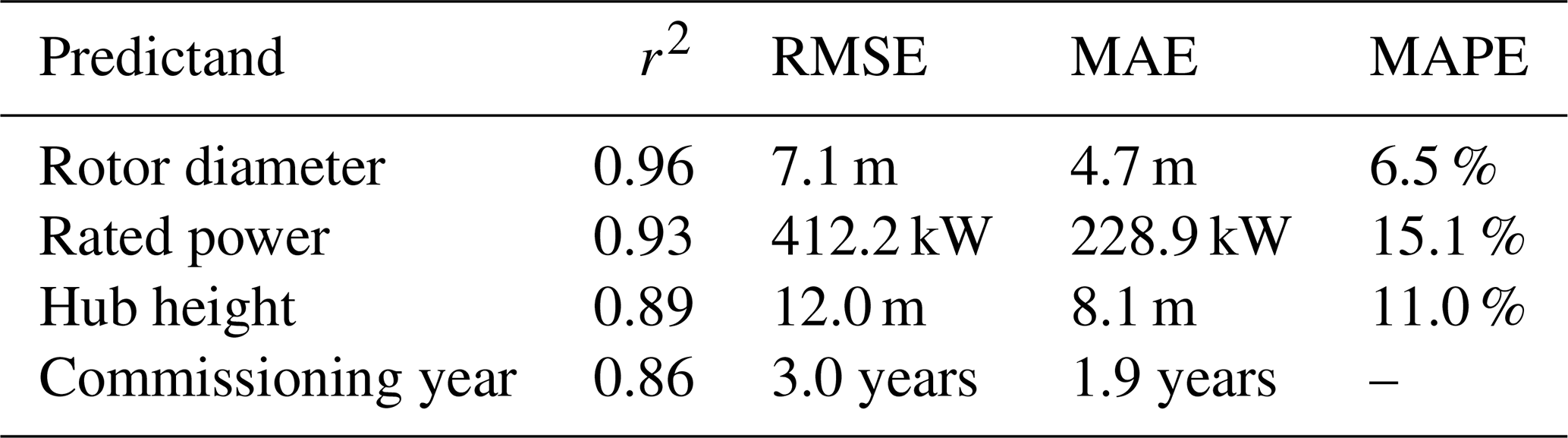
While we used the full dataset (80 % of it) to train the gap-filling models, we expect these models to be overfitted to the data (something to remedy in future versions). This occurs because numerous samples in the dataset are identical copies of the same turbine from various locations, leading to considerable redundancy. Among these, only 2937 unique combinations of rotor diameter, rated power, and hub height existed, with additional redundancy due to identical rotors being installed at varying hub heights. For this reason, over-fitting and data leakage (repeated samples in train and test data) should be a consideration. To provide a better estimate of the accuracy of the gap-filling, we carried out a cross-validation on this smaller subset of 2937 samples (instead of the whole dataset). The cross-validation consisted of randomly splitting the samples into five equally sized groups (five-fold split), training the models on four groups, holding out the last group, and then using the trained models to predict the samples in the last group (cross-validation). This is repeated five times sequentially, using all groups as the hold-out group. Only the samples where the target variable is present were used for the cross-validation. The evaluation results are presented in Table 2.

Rotor diameter and rated power are strongly correlated, each dominating the feature importance measure for predicting the other. The cross-validation shows that rotor diameter is generally accurately predicted, with a mean absolute error of 4.7 m or 6.5 %. Still, Fig. 6 shows that some larger outliers above 30 % exist. For rated power, the non-linear relationship between rotor diameter and power (and hub height and power) results in much greater errors (MAPE of 15.1 %), with rather extreme outliers (70 % and more in some cases) present in Fig. 6, especially for the lower range of rated powers. The rotor diameter is the most important feature for the model predicting hub heights, with smaller contributions from the other variables. The cross-validation shows a mean error of 8.1 m (11 %), but residuals show heteroscedasticity and a tendency for errors to be (relatively) larger for smaller heights.

2.2.6 A few insights from the wind turbine database

The WTD comprises approximately 7 % offshore and 93 % onshore turbines. Offshore turbines are newer and, on average, have 2.5× higher installed capacities. Models by Vestas, Enercon, Siemens, and Gamesa (now Siemens-Gamesa) account for two-thirds of the turbines and an even larger share of total capacity. The most common model, Vestas V90/2000, represents about 5 % of the dataset (see Fig. 7).

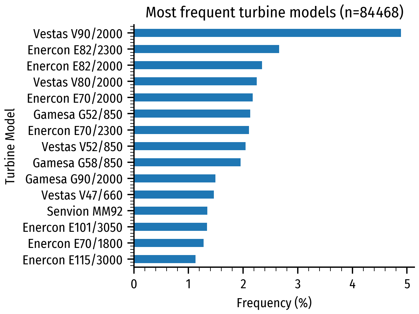
Figure 7 Frequency of turbines in the dataset after gap-filling and splitting all wind farms into individual turbine entries.

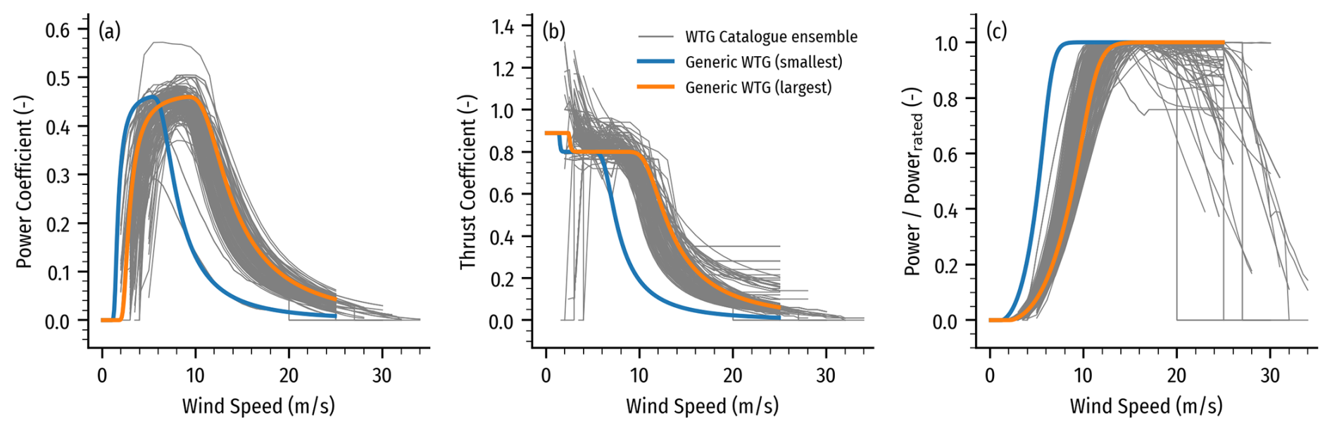
Figure 8 Turbine operational curves: (a) power coefficient curves, (b) thrust coefficient curves, and (c) power curve relative to the rated power. The grey lines show all curves for all different turbine models. The blue and orange lines show the generic curves using PyWake's standard_power_ct_curve function (PyWake-Team, 2022), respectively, for the smallest and largest turbines in the turbine dataset.

2.2.7 Turbine power and thrust curves

Turbine power and thrust curves must be known for each turbine to account for its speed-dependent drag on the wind field in the NWP model. For the 213 largest and most frequently occurring turbines (about 80 % of the turbines), we used a collection of proprietary turbine curves provided in the WindPro software (EMD International, 2023) to associate the class with accurate curves (grey lines in Fig. 8). In all cases, we used the curves representing standard operating conditions, corresponding to the normal turbine control mode and a standard air density of 1.225 kg m⁻³.

We assigned the remaining less frequent turbine models (20 % of turbines) to the generic turbine class. About $\mathrm{3}/\mathrm{4}$ of these generic turbines were assigned to this class due to being an infrequent turbine model, and $\mathrm{1}/\mathrm{4}$ were assigned due to the turbine model being unknown. For this generic turbine class, we assigned standard power and thrust curves as defined by the standard_power_ct_curve (PyWake-Team, 2022) in PyWake version 2.5.0 (Pedersen et al., 2023). We used the default settings, including wind speed cut-ins and cut-outs at 3 to 25 m s⁻¹, an air density of 1.225 kg m⁻³, a maximum power coefficient of 0.49, and a turbulence intensity of 0.1. The power curves for the individual turbines in this generic class are then calculated based on their nominal power and rotor diameter. In Fig. 8, the blue and orange lines indicate how these generic curves behave for the smallest and largest turbines in the WTD.

In some cases, the gap-filled rotor diameter and rated power were inconsistent with the associated power curve assigned to the turbine class. This would occasionally result in power coefficients exceeding thrust coefficients, causing modeling errors. So, in those cases, we limited the power (absolute or coefficient) to the lower value of the two and ensured that the power coefficient always stayed below the thrust coefficient.

3 The HARMONIE modeling system

We use the WTD (Sect. 2) within the forecasting model HARMONIE cycle 43.2.2. For our long model runs, the setup of HARMONIE corresponds to the setup used operationally at DMI until May 2024. Details of the setup are given in part 1 of this series of articles (Fischereit et al., 2024). In summary, we use a horizontal resolution of 2.5 km and 65 vertical levels running from the surface up to 10 hPa. The lowest 9 model levels, along with the rotor spans of the wind turbines in the WTD, are shown in Fig. 9. The geographical extent of the NEA domain used for the simulations is highlighted in Fig. 1. Due to the horizontal resolution of 2.5 km, multiple turbines can be present within a single grid cell, depending on the distance between individual turbines within the farm. If multiple turbines are present, their individual effects on the velocity tendency, and, depending on the parameterization, the turbulent kinetic energy (TKE) tendency, are summed up. Some more details on the WFP implementations are given below.

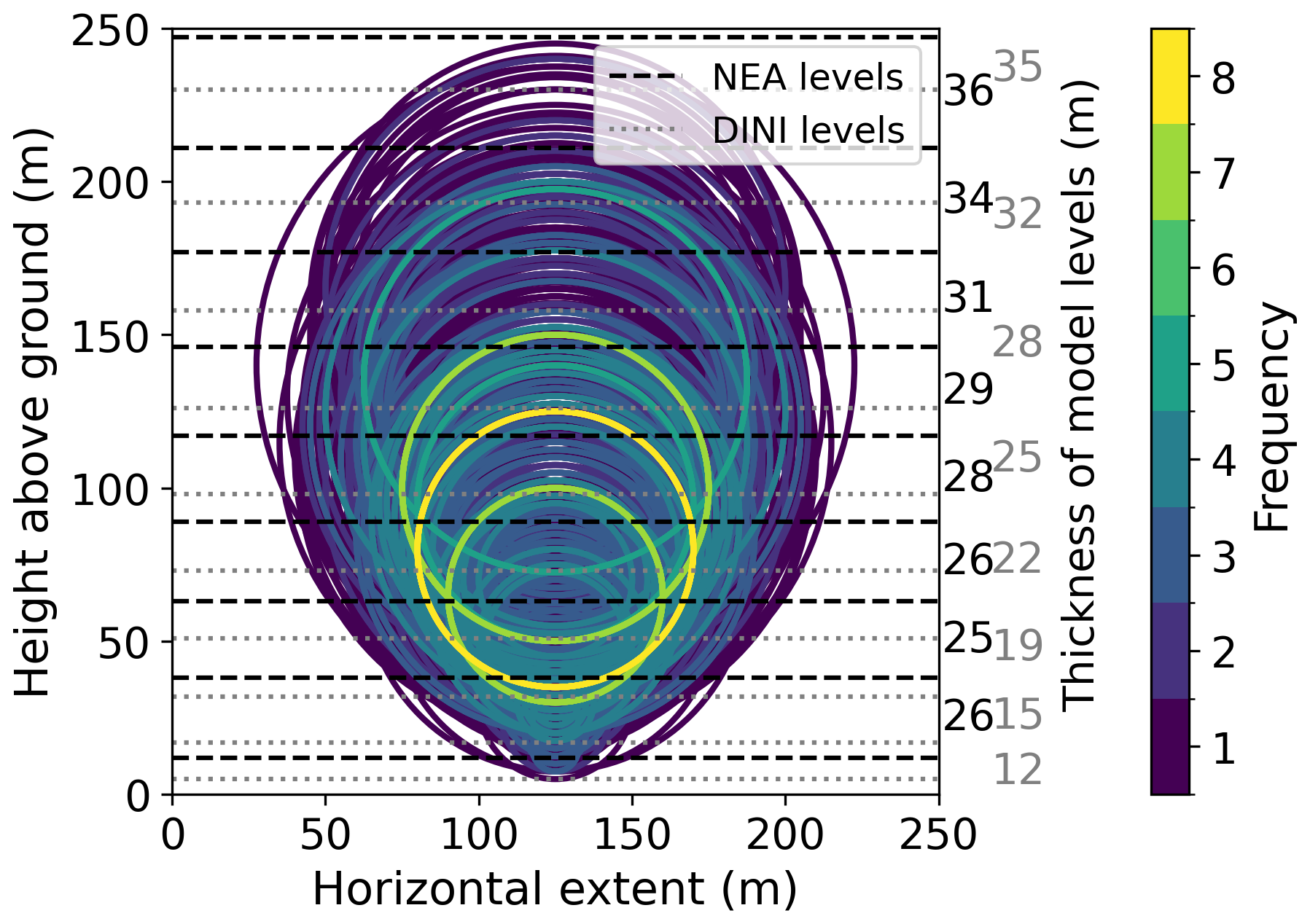
Figure 9 Height of the lowest HARMONIE model levels and turbine rotors included in the domain for the NEA simulations, color-coded by occurrence frequency in the WTD. Dashed lines show levels of the NEA domain used for our month-long simulations; dotted lines show levels of the DINI domain used in the vertical sensitivity study (Sect. 5.4). The numbers on the right indicate the thickness of each model level for NEA (black) and DINI (gray).

The HARMONIE model in the described setup is used to perform a series of sequential forecasts for two separate months: a winter month (February 2020) and a summer month (August 2022). We used the open-source CLIMatological REPresentative PERiods (CLIMREPPER) software package (DTU Wind, 2025) to assess the representativeness of the chosen periods. Overall, the combination of both months represents well the 30-year average conditions for wind speed, wind direction, and stability. In particular, compared to the climatological average, February 2020 was windier, with more westerly winds and more neutrally stratified. In contrast, August 2022 had weaker winds and more very stable and very unstable conditions than the climatological average. Therefore, putting the 2 months together resulted in conditions similar to the 30-year average. More details are given in Sect. A3.

We make 48 h long forecasts every 12 h with 3 h cycles in between for those months. This means that between 48 h forecasts, a sequence of 3 h forecasts is performed, where each forecast is initialized from the final hour of the preceding one. The purpose of this is to have more frequent data assimilation, making the NWP model stay close to the atmospheric state. Prior to these forecasts, we use an 8-day spin-up period with 3 h cycles. This long spin-up period is needed for the 3dVar data assimilation. We assimilate surface synoptic observation (SYNOP) pressures, radiosonde winds, temperatures and humidities, buoy pressures, aircraft winds and temperatures (AMDAR), and several types of surface and near-surface data. The lateral boundary conditions are taken from the Integrated Forecasting System (IFS) global model at ECMWF every hour. More details of the settings can be found in Fischereit et al. (2024).

The forecasts are run for four different scenarios, which are summarized in Table 3. One 48 h-long forecast for August 2022 without wind farms (NWF) failed. To make the analysis consistent, this forecast has been removed from all other scenarios.

Fitch et al. (2012)Volker et al. (2015)Fitch et al. (2012)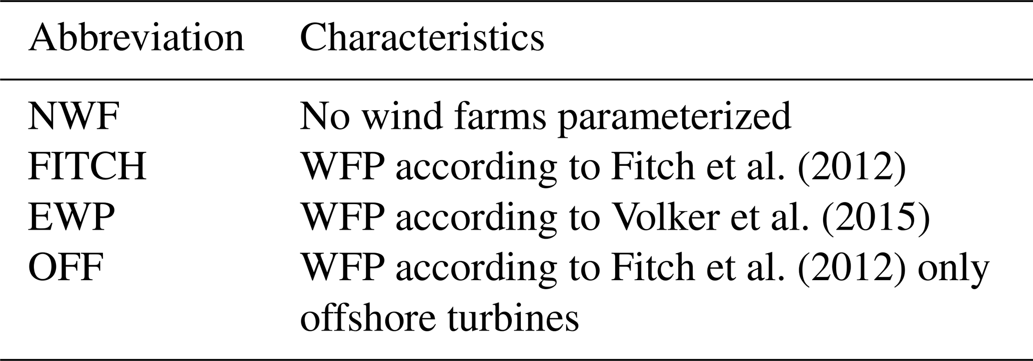

Table 3 Applied scenarios and their abbreviations.

Details of the implementation of the EWP and Fitch schemes in HARMONIE are given in van Stratum et al. (2022) and Fischereit et al. (2024). Note that the tuning parameter α that determines the relative amount of TKE injected by the FITCH WFP is set to 1 in the HARMONIE model. The HARMONIE model uses a different planetary boundary layer scheme compared to the MYNN-scheme in the WRF model, where a relative amount of α = 0.25 was recommended (Archer et al., 2020). In a recent study, Agarwal et al. (2026) found that the optimal choice of the relative TKE amount depends on the PBL scheme. Thus, the optimal choices for the WRF and HARMOINE models might differ.

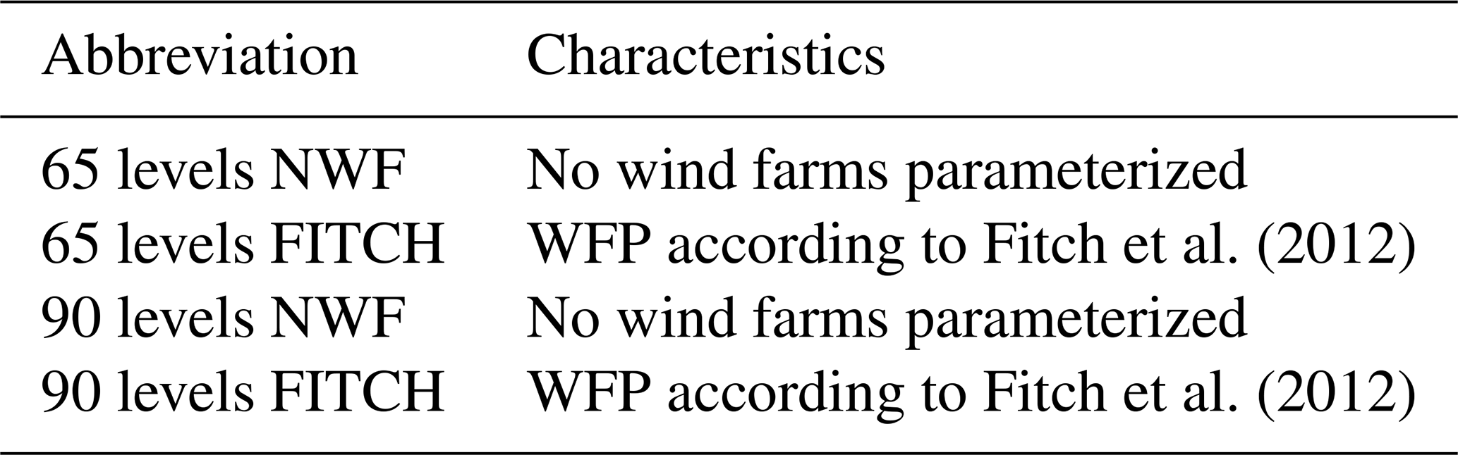
The vertical resolution of the original HARMONIE operational setup NEA is relatively coarse, with inter-layer separations ranging from 25 to 35 m in levels intersecting the rotor. Tomaszewski and Lundquist (2020) found that a coarse vertical resolution can impact the magnitude of the surface effects of operating turbines. To assess the effect of the vertical resolution, we therefore performed a sensitivity study using the higher-resolution Harmonie domain currently used operationally at DMI, called DINI, with 90 vertical levels. The DINI domain is outlined as a dashed black line in Fig. 1 and the denser vertical levels are highlighted in Fig. 9. For the larger DINI domain, we performed a set of 4 simulations (Table 4): For both the 65-level and 90-level vertical resolution, we performed simulations without wind farms (NWF) and with the Fitch parameterization (FITCH). We simulated 1 week (08.05.–17.05.2025) with 1 week of spin-up beforehand. The DINI setup is only used in Sect. 5.4, for all other forecasts we use the NEA setup.

Fitch et al. (2012)Fitch et al. (2012)

Table 4 Applied scenarios and their abbreviations for the DINI domain to study the sensitivity to the number of vertical levels.

4 Model evaluation with masts and lidars

The evaluation of the HARMONIE model forecasts with mast observations is generally very limited so far, but especially with a focus on wind energy applications. Kangas et al. (2016) developed a verification system with several masts in Europe. However, they focused on the evaluation of radiation fluxes, which are not directly relevant for wind energy applications, and only included early spring 2014 as the evaluation period. Kalverla et al. (2019) evaluated three different weather models, among them HARMONIE, against mast and lidar observations at the Dutch offshore site IJmuiden for 30 cases. They found that the HARMONIE-derived wind profiles had the smallest wind speed bias out of the three models, but, like the other models, performed worse during stable conditions. van Stratum et al. (2022) evaluated the performance of a one-year HARMONIE simulation with the Fitch WFP close to existing wind farms using both lidar and mast measurements. They concluded that the inclusion of a WFP clearly improved the model simulations close to wind farms. However, they also highlighted that in some areas, the background meteorological conditions were not well captured. The same issue was highlighted in the first part of this paper series (Fischereit et al., 2024) for selected case studies with aircraft measurements.

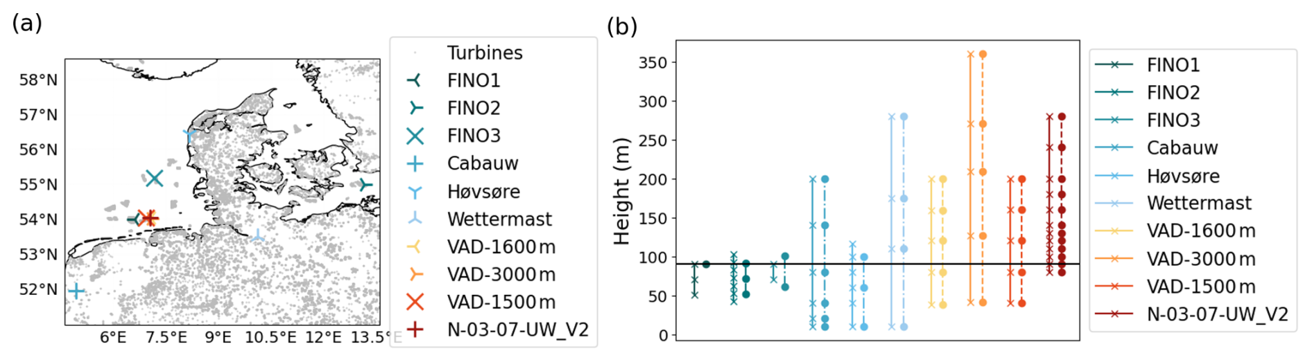
Figure 10 (a) Locations of the observations (blueish colors for masts, reddish colors for lidars) used for validation. (b) Measurement heights for wind speed (solid lines with crosses) and wind direction (dashed lines with dots) following filtering of heights with too low data availability (see text). Horizontal black line indicates height of the wind-rose bias plots in Fig. 13.

Table 5 Availability [%] of observations for the 2 months at the six masts and four lidars for all heights.

Here, we used measurements from 6 masts (3 offshore (the Forschungsplattformen in Nord- und Ostsee, FINO 1,2,3) and 3 onshore (Cabauw, Høvsøre and Hamburg Wettermast)) located in Denmark and Northern Germany and 4 lidars installed in the German Bight (Fig. 10a) to evaluate the performance of the HARMONIE model forecasts for the two selected months in this study. The lidar datasets were downloaded from the data hub of Preliminary Investigation of Sites (PINTA portal) provided by the Bundesamt für Seeschifffahrt und Hydrographie (BSH) and were part of preliminary site investigations for the new wind farm development areas N-3.7 and N-3.8 east and west of Gode Wind 1. Two different lidar types were used. Two Streamline XR lidar were placed on a wind turbine in the west of Gode Wind 1 (VAD-1500m) and on a transmission station in the east of Gode Wind 1 (VAD-1600m, VAD-3000m), respectively. A Velocity Azimuth Display (VAD) scanning pattern with several azimuth positions and different distances from the lidar position (1500 m towards west, 1600 and 3000 m towards east) and defined elevation angles between 40 and 200 m was performed to retrieve radial wind speeds and derive wind speeds and wind directions from those. In addition, a Windcube V2 lidar was placed on the transmission system, which measured the vertical wind profile in 80 to 280 m height close to development area N-3.7 (N-03-07-UW_V2). More lidar measurements were performed, but were not analysed here, since they probed the atmosphere in similar areas. More details on the performed measurements can be found in Neumann et al. (2020).

Measurement heights are shown in Fig. 10b for wind speed (solid lines with crosses) and wind direction (dashed lines with dots). Basic data cleaning was performed for all measurements, including the removal of flagged data, and tests for plausibility and for flat line following Ramon et al. (2020). The cleaning is performed on individual heights. The different datasets can be accessed as described in the “Code and data availability” section.

4.1 Average profiles

We interpolate the forecasts with the different scenarios (Table 3) to the location and height of the measurement, and average the wind speed and direction for all forecasts and all lead times (Sect. 3). For each measurement location, any timestamps missing at one height are removed from all heights and from the corresponding forecasts to ensure consistent wind profiles with the same timestamps in all heights. If a height has 10 % lower data availability than the others, it is removed entirely to maximize the overall mean data availability rate. Table 5 shows the availability of wind speed after cleaning for the 2 months for the masts and the lidars, respectively, and Fig. 10b shows the heights after filtering.

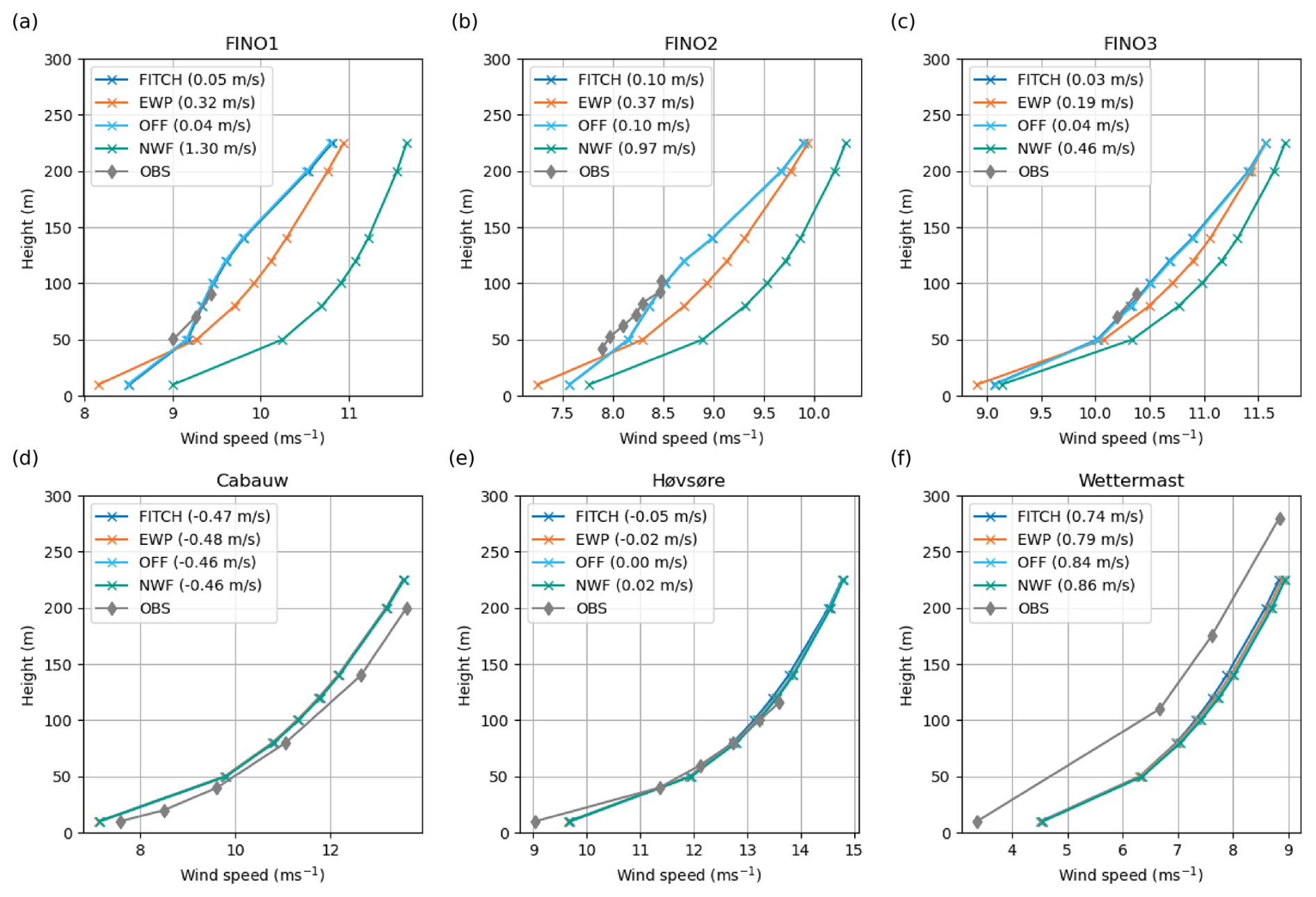
Figure 11 Time-averaged profiles from the forecasts and from mast measurements for both months. Mean biases over all heights are shown for the different scenarios. Note that the x axis varies from site to site and FITCH and OFF are almost identical.

Figure 12 Same as Fig. 11, but for the lidar sites.

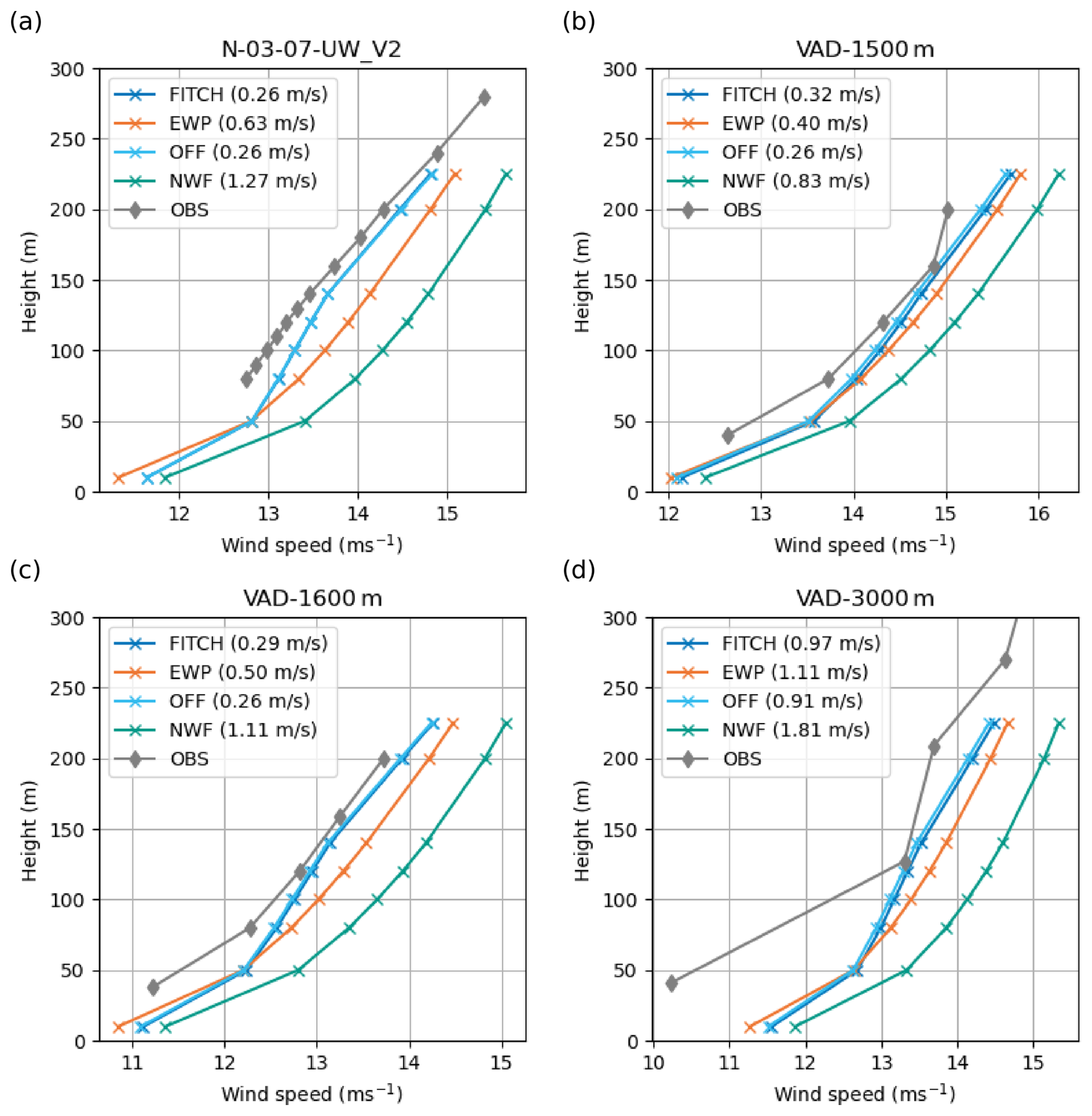
The comparison between the forecasts and measurements for the wind speed is presented in Fig. 11 for the masts and Fig. 12 for the lidars. The legend entries show the mean biases over all heights for the different scenarios and sites. Overall, the forecasts agree well with the observations, especially the FITCH scenario. Largest differences are visible for Hamburg Wettermast, where wind speeds are overestimated by around 0.8 m s⁻¹ at all heights, and Cabauw, where wind speeds are underestimated by around 0.4 m s⁻¹. For those two masts and for Høvsøre, all simulation scenarios are almost identical, since there are no big wind farms located in their direct vicinity.

At the sites that are strongly influenced by wind farms, i.e., the FINO masts and lidar sites, the forecasts without wind farms (NWF) clearly overestimate the wind speed (Figs. 11 and 12). To quantify this effect, biases are derived by linearly interpolating to the measurement heights and subtracting the measured wind speed from the simulated wind speed. The biases, as given in the individual legend entries, show that from the winds simulated by two wind farm parameterizations, the forecasts with the WFP by Fitch et al. (2012) FITCH and OFF are closer to observations than EWP for all sites. FITCH and OFF are almost identical at the offshore sites, indicating that the effect of onshore turbines is minimal on average. It is interesting to note that the wind profiles from the various scenarios do not converge to the same value for the wind farm-influenced site even at 300 m above ground.

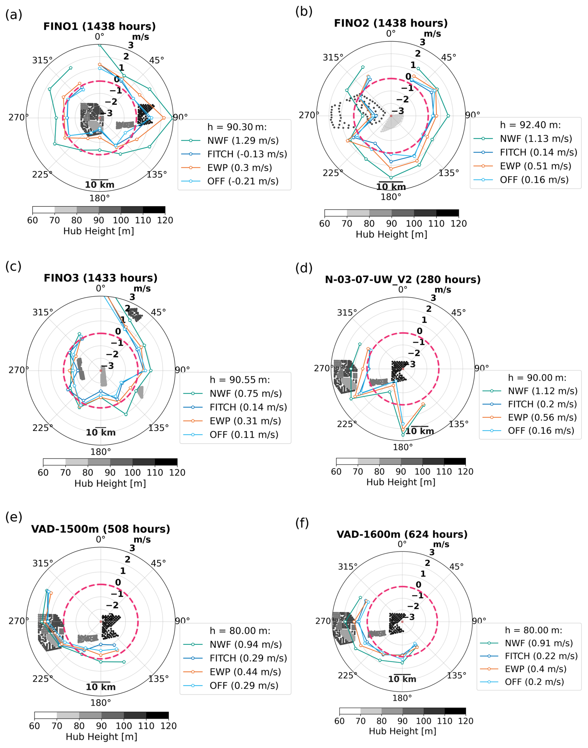
Figure 13 Directional bias (simulation minus measurements) of the different simulation scenarios (colored lines) for measurement sites close to wind farms. Bold dashed magenta circle highlights zero bias. Lines within the magenta circle indicate negative biases, while lines outside indicate positive biases. The averaged bias over all directions is shown in the legend. Dots show the location and hub height of wind turbines in the vicinity of each site, which is shown as a red dot in the center of the plot. The total duration of observational data for each site is shown in the subtitle. Sectors with fewer than 10 occurrences in either the observations or the simulations are not shown.

4.2 Wind-rose biases

The largest effects of the wind farm parameterizations are expected downwind from wind turbines close to hub height. Thus, in addition to the mean profiles in Figs. 11 and 12, directional biases are calculated and shown in Fig. 13 for the sites in close proximity to wind farms. The observations were cleaned to ensure that both wind speed and wind direction at a height close to 90 m are available for a particular time stamp. A height of 90 m has been chosen, since many observations are available around this height (Fig. 10b) and it is close to hub height of older offshore turbines. Note that for some masts, wind speed and wind direction are measured at slightly different heights (Fig. 10b). After the cleaning, the mean wind speed for each sector is computed using the data for each scenario and for the observations binned in 30° wind direction sectors. Figure 13 shows the difference between the measured and observed mean wind speeds for each scenario in each sector.

The wind-rose biases highlight again that the forecasts using a wind farm parameterization generally perform better close to the wind farms since they are closer to the magenta dashed zero-bias circle in Fig. 13. Averaged over all wind directions, the simulations using WFP by Fitch et al. (2012) show the smallest bias again (see legend entries) for all sites.

For some wind directions, the NWF scenario already underestimates the wind speed (see e.g. 180° at FINO1). Thus, already the background meteorology is not well simulated for that particular site and direction. Adding the wind farm parameterization to those forecasts causes an even larger underestimation of the wind speed due to the wake effect. Similar challenges have been reported in other studies already, as discussed above.

FINO2 is a special case since the wind turbines of Kriegers Flak, which are visible to the west of FINO2 in Fig. 13b, were built in September 2021, i.e., in between the simulations for February 2020 and August 2022. However, since the same wind turbine database from November 2021 (Sect. 2) is used for both months, FITCH and EWP naturally underestimate the wind speed from that sector. But also NWF underestimates the wind speed from that direction, indicating that the background meteorology is again not well matched. The same issue exists for Fig. 11, but is less prominent, since an average over all wind directions is shown.

Table 6 Area in km² with reduced wind speed ΔWS due to the presence of the wind turbines SCEN−NWF. For comparison, the area of Denmark is 43 000 km².

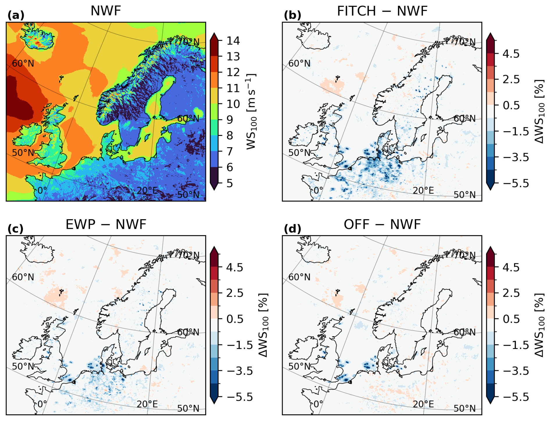
Figure 14 (a) Average wind speed at a height of 100 m for February 2020 and August 2022 for the simulation without wind farms (NWF) and normalized difference with respect to NWF to simulations with (b) FITCH WFP, (c) EWP WFP and (d) FITCH WFP for offshore turbines only.

5 Results

5.1 Wind turbine impacts on wind forecasts

Figure 14a shows the simulated wind speed at a height of 100 m averaged over all forecasts for both February 2020 and August 2022 for the scenario without wind farms (NWF). Characteristic higher wind speeds are visible over the sea, coastal areas, and mountainous areas. The wind turbines are imprinted in the FITCH simulations as areas of lower wind speeds (Fig. 14b) both on- and offshore. Compared to FITCH, EWP calculates smaller wind speed differences that cover smaller areas (Fig. 14c). This can also be seen from Table 6, where the wake-affected area based on different thresholds of relative differences between the scenarios with wind farms and the scenario without wind farms is shown. This finding agrees with previous studies (e.g. Fischereit et al., 2024; Pryor et al., 2020). The more vague differences in wind speeds in areas without wind farms are discussed at the end of this section.

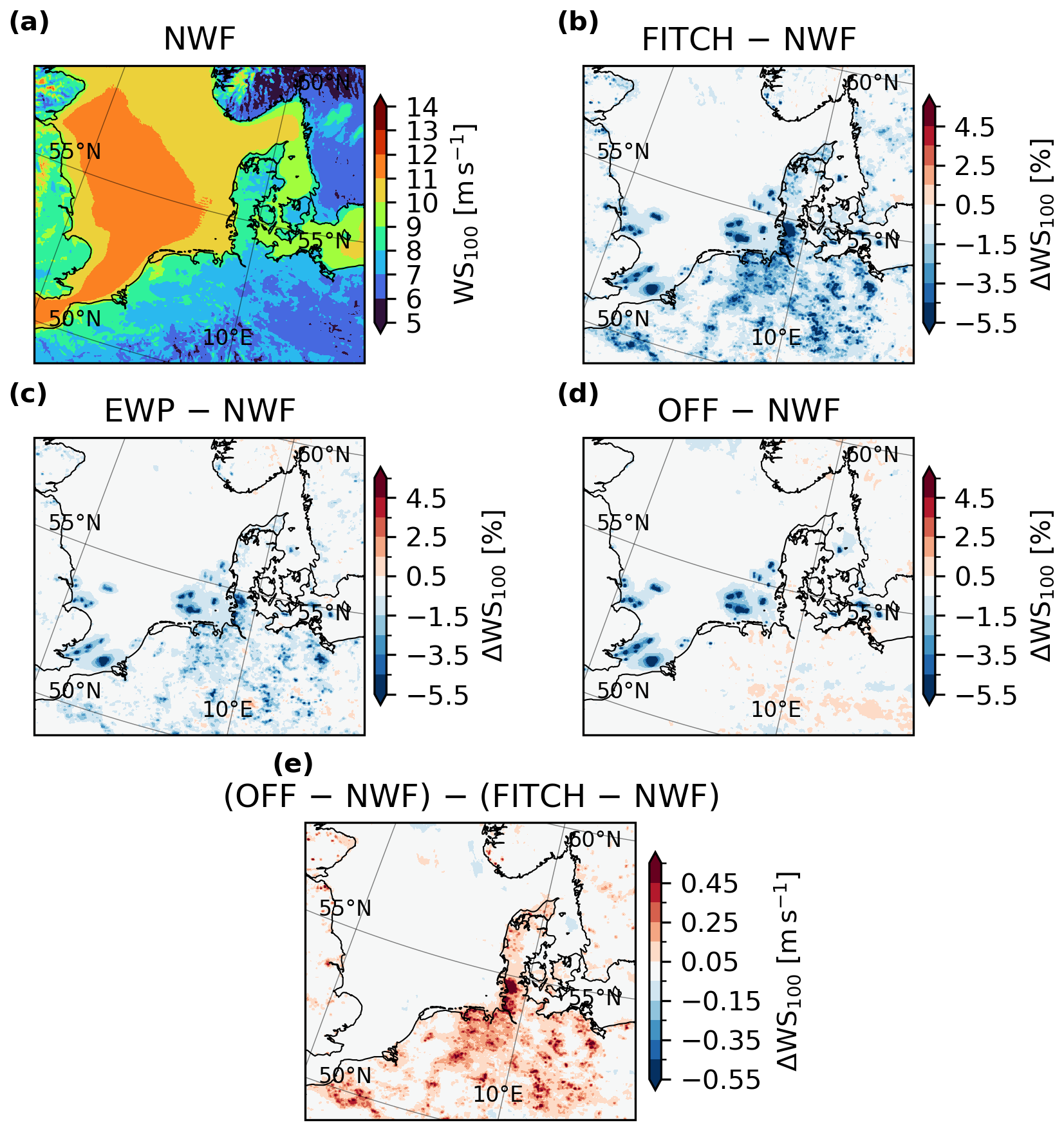
Figure 15 (a) Average wind speed at a height of 100 m for February 2020 and August 2022 for the simulation without wind farms (NWF) and normalized difference with respect to NWF to simulations with (b) FITCH WFP, (c) EWP WFP, (d) FITCH WFP for offshore turbines only and (e) the absolute difference between (d) and (b); zoom into the North Sea and Danish Baltic.

Excluding onshore turbines vastly overestimates wind resources onshore (Fig. 14b vs Fig. 14d). Figure 15 presents a zoomed-in version of areas with high wind turbine built-out, the North Sea, the Danish part of the Baltic Sea, and northern Germany, and also includes the difference between the two FITCH scenarios that only differ in the inclusion of onshore turbines (Fig. 15e). This also highlights, in absolute numbers, that the wind resources are greatly overestimated onshore if only the offshore turbines are included. Hence, onshore turbines should be included for accurate power forecasts for all European turbines. The impact of missing onshore turbines stretches a bit offshore in the German Bight, thus affecting also the power forecast for near-shore turbines. However, there are no systematic long-distance remote effects and thus power forecasts for wind farms further offshore are not affected on the 2 month average by not including onshore turbines, as could also be seen in Sect. 4 for the studied offshore sites. While wind deficits from onshore turbines can be quite strong, they especially contribute to waked areas < 1.5 % and < 3 % and less to wake areas with deficits smaller than 5 % (Table 6). This is because of the faster wake recovery onshore, which rapidly reduces peak wind deficits at the wind farms. Individual wind farms are “connected” through areas of lower wind speeds, both for FITCH and EWP. This indicates that already under the current built-out, these wind farms affect each other's wind resources. Thus, wind farm wake effects must be considered for accurate power forecasts.

Differences between the forecasts with and without wind farms are visible also in regions without wind farms, e.g., south of the Faroe Islands in Fig. 14. Those differences are mostly < 1.5 % and are of a random nature. It is expected that for longer averaging times, those differences will vanish completely, and only the wind farm effect signal will be left. This can be seen by comparing the two-month average in Fig. 14 to the averages of the individual months (Sect. A4), where the differences are much bigger. These areas of different wind speed arise because differences between the model simulations linked to weather systems and their associated fronts are slightly displaced between the simulations. This effect is seen most clearly in areas with few observations, where the data assimilation has a weaker impact, enabling the simulations to drift further apart. Since February 2020 was relatively stormy (Sect. A3), areas of higher and lower wind speeds are also imprinted on the two-month average in Fig. 14. From a weather forecasting point of view, these differences are considered noise because they are random and not systematic (see analysis in Sect. 5.2). In that way, they act as a perturbed ensemble member outside the wind farm area.

5.2 Statistical significance of wind speed changes by wind farms

While there is a strong systematic impact of the wind farms on the wind speed at a height of 100 m, it remains unresolved whether these differences (Sect. 5.1) are actually statistically significant or could arise by chance. Since the data is auto-correlated both spatially and temporally, and the underlying distribution is not known, standard significance tests, like Student's t-test, cannot be applied. Instead, we implemented the significance test suggested by Wilks (1997) and Marchand et al. (2006). The tests rely on bootstrap resampling of blocks of a particular length. We describe the method in brief in Sect. A5.

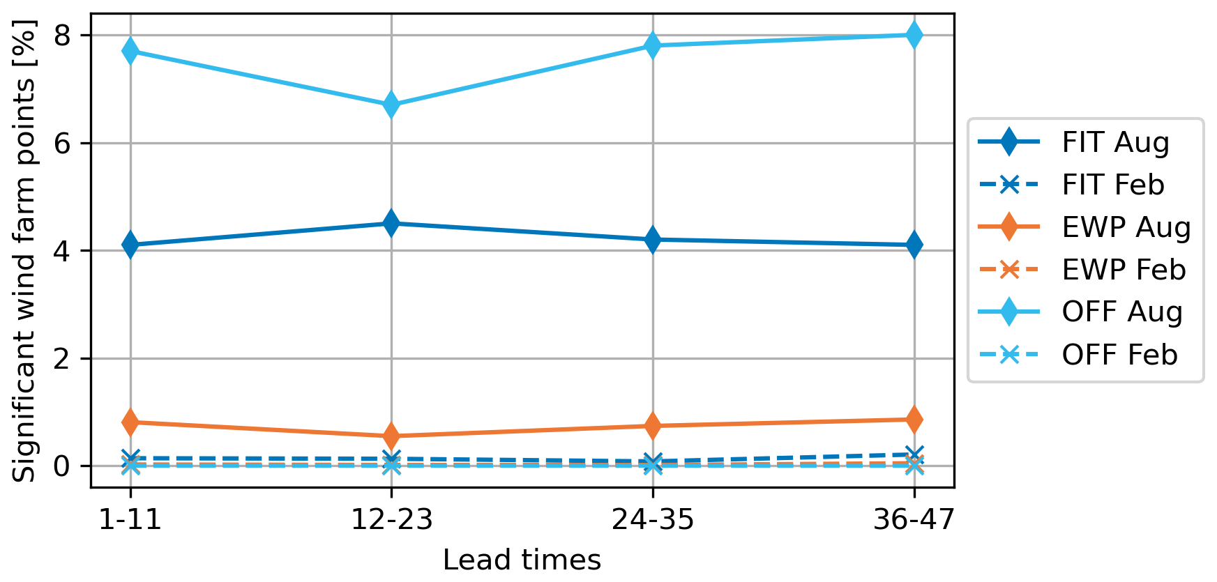
Figure 16 Relative number of significant grid points with respect to the number of grid points with wind turbines for different lead times for different scenarios (colors) and the 2 months (solid lines are August 2022 and dashed lines are February 2020).

To apply the described method, the first step is to produce a continuous time series of the forecast data. For that, the forecasts are split into different lead times: 1–11, 12–23, 24–35, 36–47, separately for February 2020 and August 2022. This gives four continuous time series for each month. We then calculate the block length for each lead-time. Using these pre-calculated block lengths, we perform the bootstrap resampling for each of the three scenarios, (1) FITCH, (2) EWP, and (3) OFF, and NWF, respectively. To test how many bootstrap samples n_b are required, we tested n_b = 2500, 4000, 7500, 10 000 for one scenario (FITCH) and one lead time (1–11) and calculated the number of significant grid points relative to the number of grid points with wind turbines. Thus, this ratio shows, for how many grid points with wind turbines in the domain, the WFP has a statistically significant effect on the modelled wind speed. The results are relatively stable around 4 % for all tested values of n_b. This means that the number of significant grid points doesn't change much for the tested number of bootstrap samples. Thus, to limit computational costs, we chose 4000 for all lead times and scenarios.

The number of significant grid points with respect to grid points with wind farms is also relatively constant for all lead times (Fig. 16). Overall, August has more significant points than February due to the stormier conditions and smaller wake effects in February 2022 (Sect. A3).

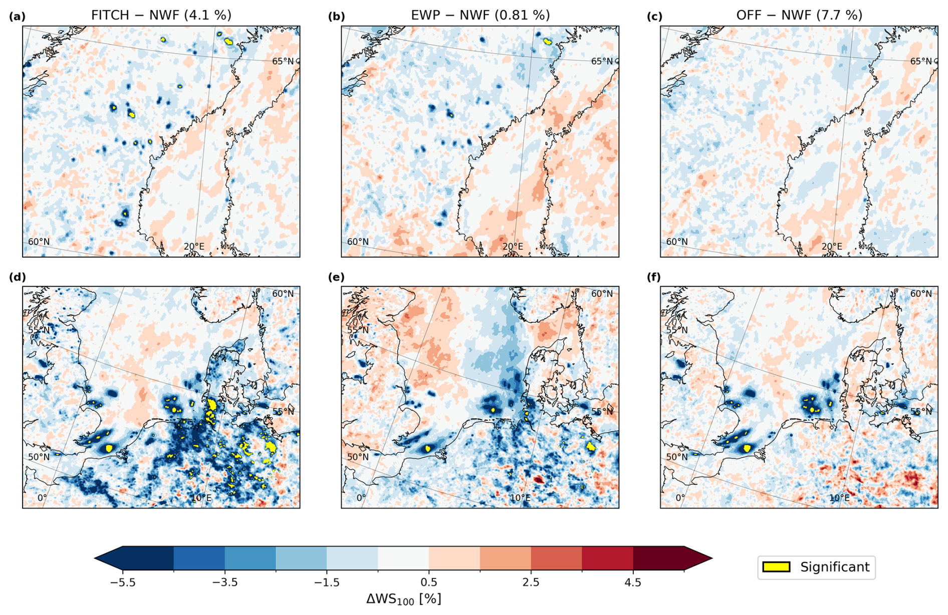
Figure 17 Statistically significant grid points (yellow) for the three scenarios with wind farm parameterizations (FITCH, EWP, OFF) compared to the NWF scenario for the lead time 1–11 h for August 2022 for (a,b,c) focusing on Northern Sweden and (d,e,f) focusing on the North Sea region and the Danish Baltic. The percentage number shows the number of significant grid points relative to the number of grid points with wind turbines for the entire domain. Colors in the background show normalized differences with respect to NWF for the different wind farm parameterizations.

The results for the lead time 1–11 h for August 2022 for the three scenarios are shown spatially in Fig. 17 as yellow areas. Statistically significant differences exist both for onshore and offshore farms for FITCH (Fig. 17a and d). Overall, a smaller number of significantly different grid points were found for EWP. The percentages are calculated based on the number of statistically significant grid points compared to the number of grid cells with wind farms. This latter number is significantly smaller for the scenario “OFF”, which leads to higher relative values compared to FITCH. Overall, the significant areas are quite small. However, if comparable results were found for forecasts longer than one month, the size of the statistically-significant areas would grow. The background wind speed in 100 m height is quite patchy, since we only use 1 month of data for averaging compared to 2 months with 48 h forecasts every 12 h in Sect. 5.1. However, as this test shows, these effects are of a random nature and not statistically significant, and thus would disappear for longer averaging times.

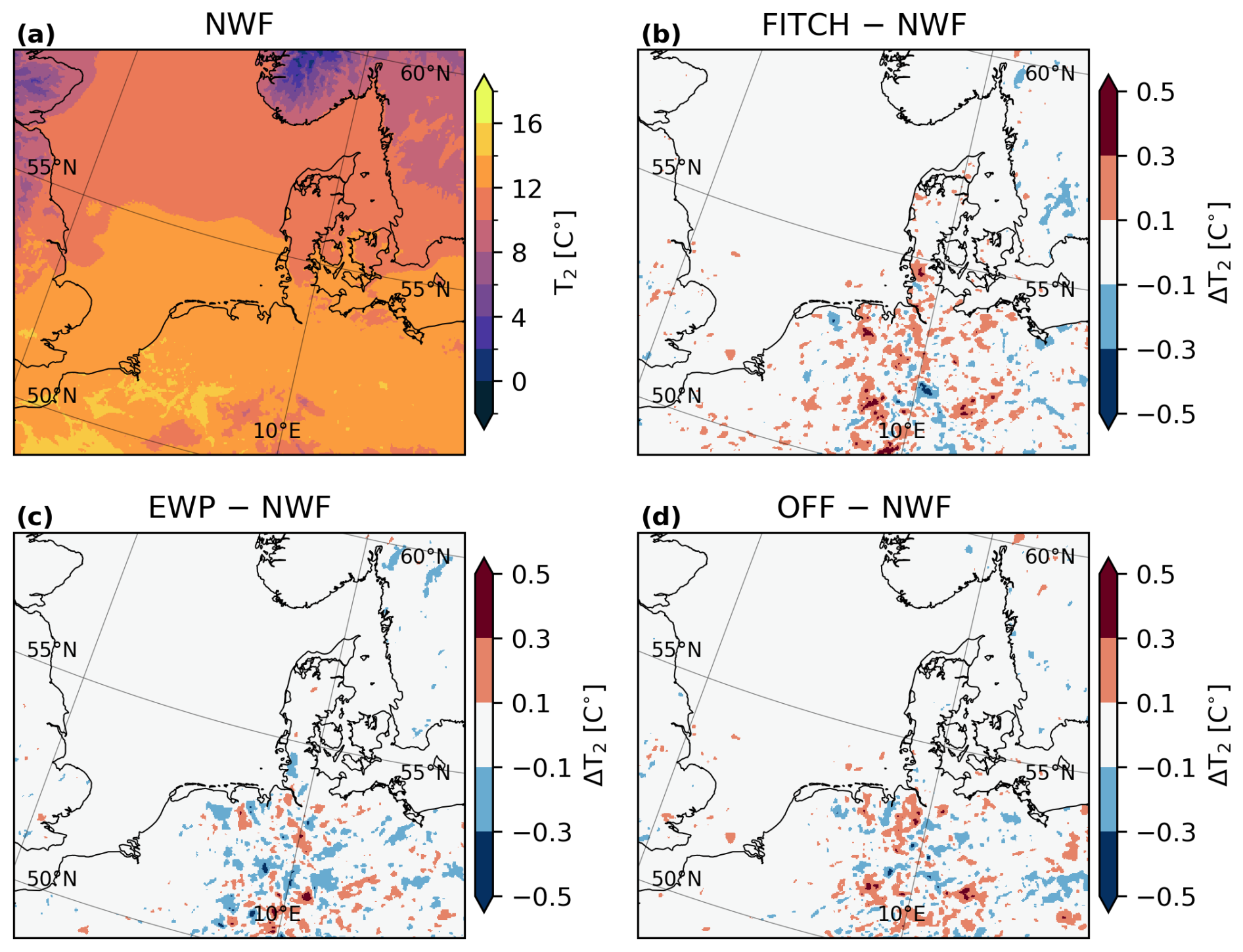
Figure 18 (a) Average 2 m temperature for February 2020 and August 2022 for the simulation without wind farms (NWF) and difference to simulations with (b) FITCH WFP, (c) EWP WFP and (d) FITCH WFP for offshore turbines only zoomed into the North Sea and Danish Baltic.

5.3 Impacts on 2 m temperature

Figure 18 shows the average 2 m temperature for NWF for all forecasts during February 2020 and August 2022 combined. Overall, the magnitude of the mean temperature differences due to the presence of the wind farms is small, i.e., ΔT₂ < ± 0.75 K for the 2-month average (Fig. 18b-d) and mostly confined to land areas. These impacts found in the HARMONIE model simulations are similar, but slightly bigger than the temperature impacts found by Quint et al. (2025) in the WRF model for their case with 100 % of TKE added. Comparing to this scenario makes sense, since in HARMONIE the amount of TKE added by the WFP is always 100 % (Sect. 3). The temperature impact is likely bigger in the HARMONIE simulation because smaller turbines are used in our simulations: Golbazi et al. (2022) found that smaller turbines exhibit surface warming, while bigger turbines produce less warming or even cooling depending on the amount of added TKE (Golbazi et al., 2022; Quint et al., 2025).

Systematic warming is detected below the big offshore wind farms in the North and Baltic Sea for FITCH (Fig. 18b and d). However, also many patches of warming and cooling can be seen over land, even when comparing the scenario without onshore turbines to the NWF scenario (OFF – NWF, Fig. 18d). The differences between OFF and NWF over land are likely due to noise, i.e., slight differences in incoming radiation due to differences in clouds in NWF and OFF. Applying the same significance test as in Sect. 5.2 to 2 m temperature, no significantly different areas were found for the 2 months individually for the full day.

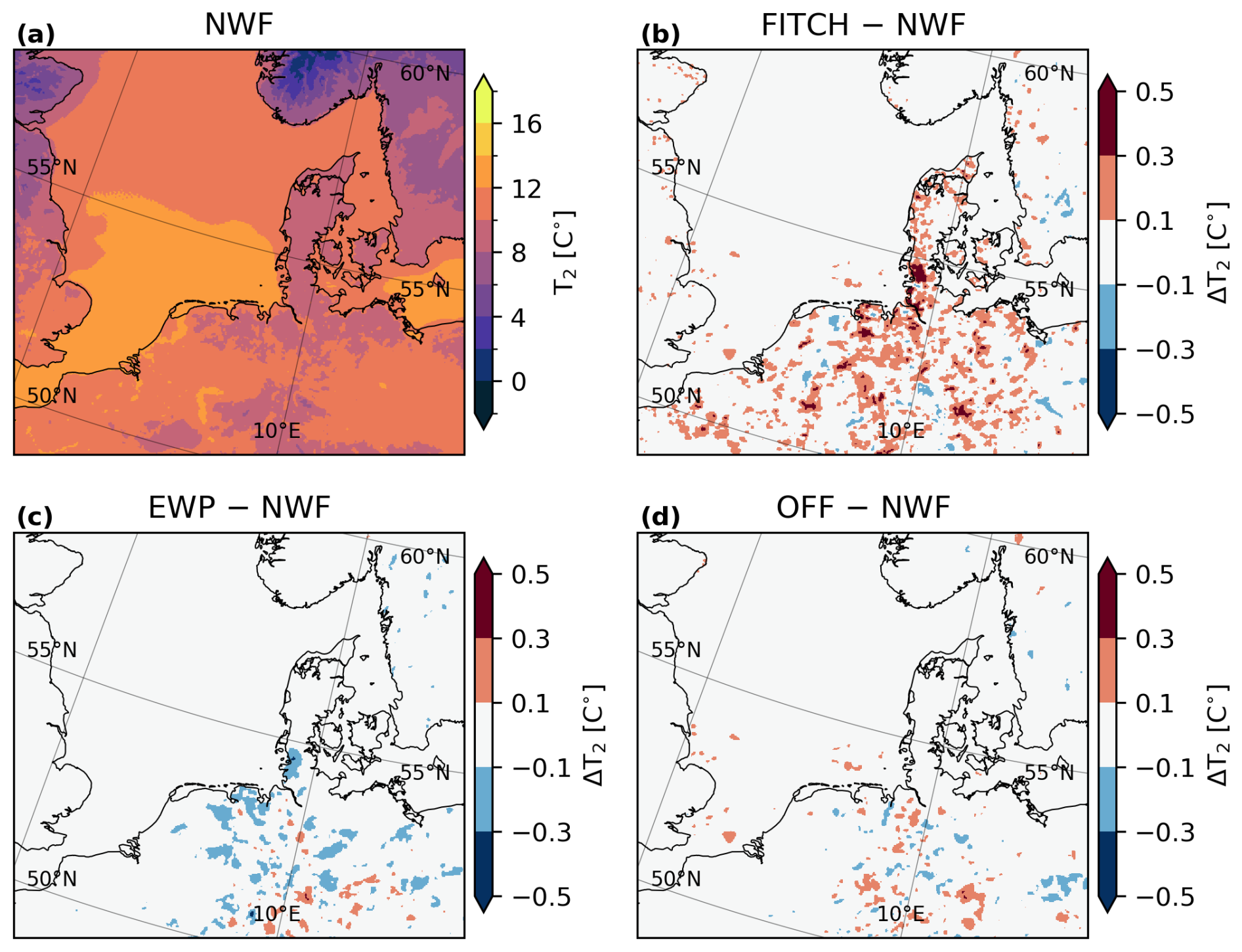
Figure 19 As Fig. 18, but averaged during nighttime (00:00–04:00 UTC) conditions only.

The systematic warming is even more pronounced under nighttime conditions, defined as the average between 00:00 and 04:00 UTC (Fig. 19b and d). This is in line with previous studies as summarized in Sect. 1. During nighttime, the noise effects onshore in OFF are less extensive (Fig. 19d), compared to all day (Fig. 18d) and especially daytime (12:00–16:00 UTC, Fig. A8d), indicating that the differences onshore are likely due to differences in incoming radiation.

Comparison of the results for EWP and FITCH shows differences offshore: Although FITCH shows warming on average below the wind farms, as discussed previously, EWP does not show any effect. This is likely due to the lack of explicit mixing in EWP compared to FITCH, since enhanced mixing in the upper part of the rotor area is an important driver of temperature changes near the ground (Xia et al., 2019; Wu and Archer, 2021; Quint et al., 2025, Sect. 1). Furthermore, onshore opposing effects are simulated with EWP, especially at night (Fig. 19b and c): EWP overall simulates more cooling, while FITCH simulates more warming. It is difficult to determine which parameterization is correct, since “control” measurements without turbine effects do not exist. However, current literature seems to agree that during stable conditions, a warming effect near the surface is expected (Sect. 1), indicating that an explicit TKE source should be added to EWP to be able to simulate those effects.

5.4 Sensitivity with respect to the number of vertical model levels

Tomaszewski and Lundquist (2020) used WRF model simulations to investigate the effect of the vertical model resolution by comparing results with 10 and 30 m resolutions. Their study found that they could only reproduce the nighttime warming in the simulations with 10 m vertical grid spacing, while 30 m grid spacing caused a cooling effect. Although we already see nighttime warming with the NEA set-up used for the preceding analysis, we investigate whether the temperature impacts found remain the same with increased vertical resolution.

The HARMONIE NEA set-up that we have used in the analysis so far has a relatively coarse vertical resolution, ranging from 26 to 36 m in the height covered by wind turbine rotor area (Fig. 9, black dashed lines). To test the impact of higher vertical resolution, we use the currently operational DINI setup, which has slightly more vertical levels than NEA: 90 as opposed to 65. This results in layer thicknesses ranging from 12 to 35 m in the rotor area (Fig. 9, gray dotted lines). It would have been ideal to introduce even more additional levels, but because of the resources required to calculate new structure functions for the data assimilation system when the resolution is changed, that was not feasible in practice. Details of the DINI setup and scenarios are given in Table 4.

Figure 20 shows the difference in 2 m temperature of FITCH – NWF for 65 levels and 90 levels. As discussed previously (Sect. 5.1), the differences between FITCH and NWF in regions far from the direct impact of wind farms likely arise from small differences propagating through the model and are expected to disappear if averaged over longer. As this analysis averages over only a week, they are larger here than for the month-long simulations. Similarly, the differences between the 65- and 90-level results in these regions are unlikely to have physical significance.

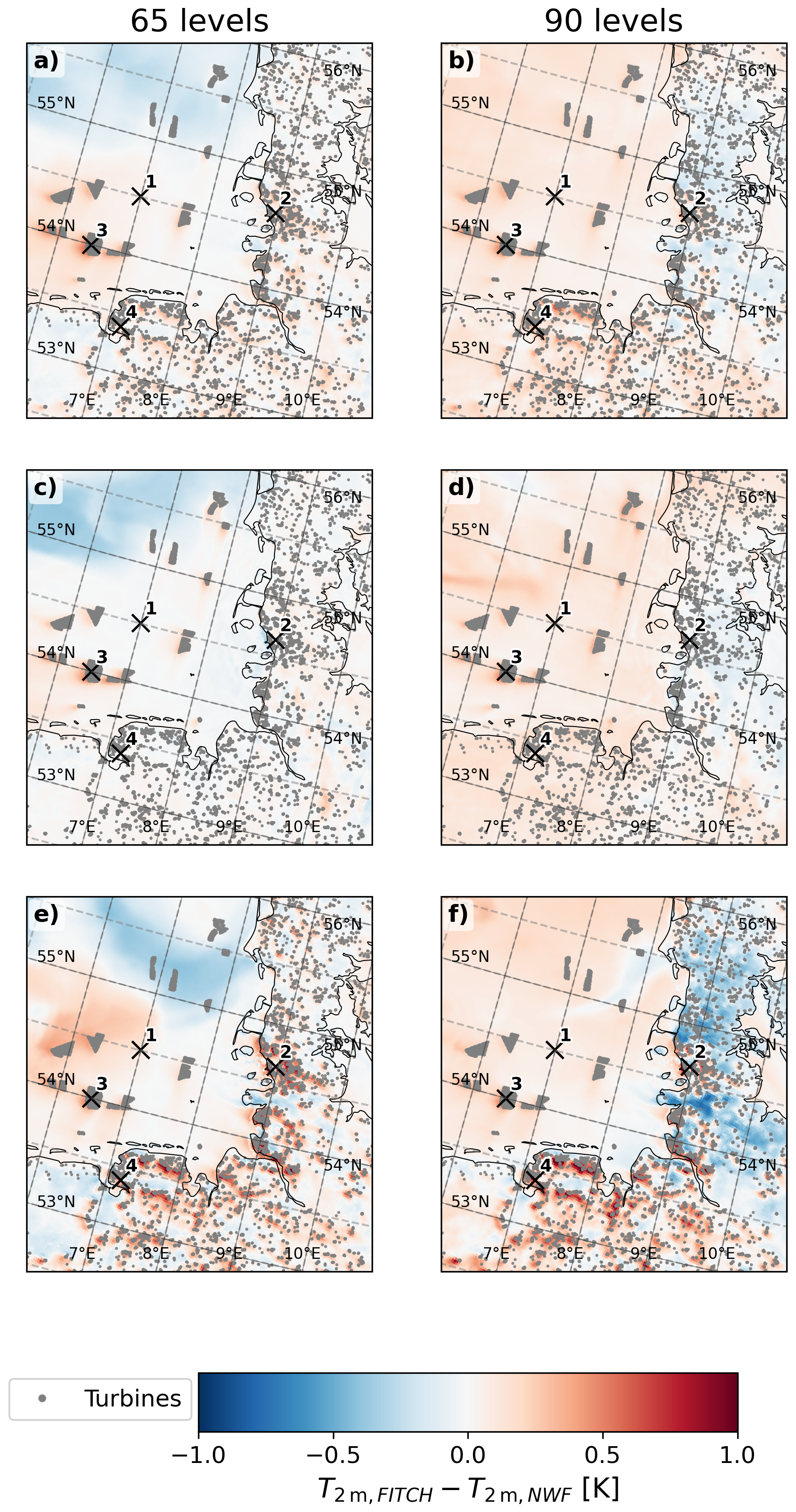
Figure 20 2 m temperature difference for FITCH-NWF for (a, c, and e) 65 levels and (b, d, and f) 90 levels averaged (a, b) over the full week 8–17 May 2025 and (c, d) over daytime (12:00–16:00 UTC) and (e, f) over nighttime conditions (00:00–04:00 UTC) only. Turbines are shown as gray dots, and the four crosses highlight locations used in Fig. 21.

However, the focus here is to look at the effect of wind farms in their vicinity. Comparing the wake areas, the same temperature patterns can be observed for both level configurations: warming in the wake of most offshore farms during all averaging times and warming of onshore turbines, especially during the night. Thus, the conclusions in Sect. 5.3 are confirmed by the simulations with more levels across the rotors.

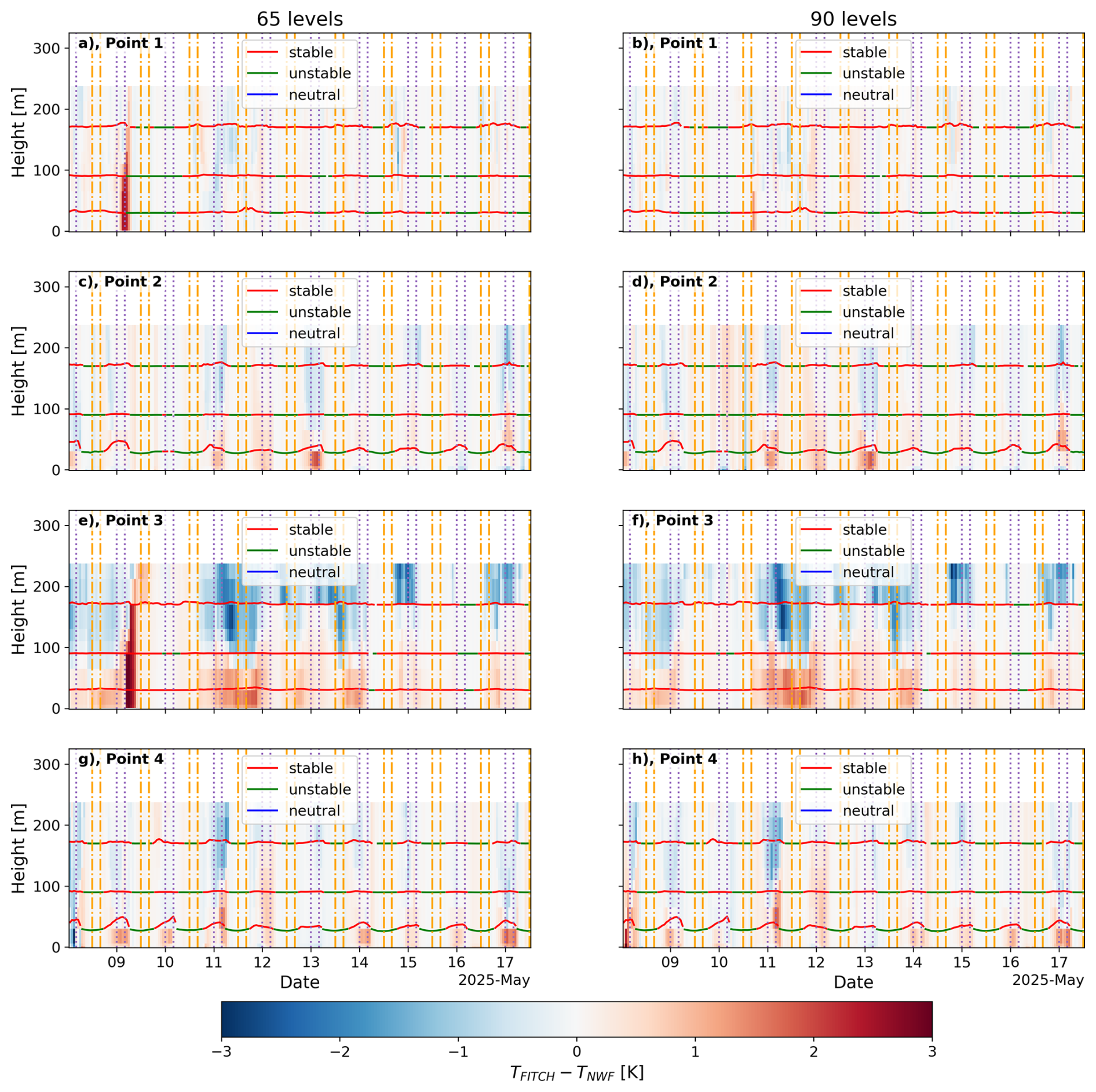
Figure 21 Timeseries of temperature profile difference of FITCH minus NWF for four points (rows) highlighted in Fig. 20 for the (a, c, e, and g) 65 levels and (b, d, f, and h) 90 levels. The background color shows the temperature difference at each altitude and date. The horizontal lines highlight the color-coded virtual potential temperature gradient (γ)-derived stability for three heights (10–50, 80–100 and 140– 200 m) and shown at the center of these layers. Purple dotted vertical lines highlight periods used for nighttime averages (00:00–04:00 UTC) and orange dash-dotted vertical lines highlight daytime average periods (12:00–16:00 UTC).

To look into more detail, Fig. 21 shows time-series of profiles of the temperature difference between FITCH and NWF during the simulated week for 4 locations, which are highlighted in Fig. 20. Point 1 is an offshore point far away from wind farms, point 2 is an onshore point in an area with surface warming in Northern Germany, point 3 is located within an offshore wind farm area, and point 4 is located onshore close to the coast in Northern Germany. In addition, the static stability at three heights is calculated using the virtual potential temperature (θ_v) gradient γ (Eq. 1) following Platis et al. (2022), who found this to be a robust measure for stability in the German Bight:

$$\begin{array}{}\text{(1)}& {\displaystyle }& {\displaystyle }\mathit{\gamma }\approx {\displaystyle \frac{\mathrm{\Delta }{\mathit{\theta }}_{\mathrm{v}}}{\mathrm{\Delta }z}}\text{(2)}& {\displaystyle }& {\displaystyle }{\mathit{\theta }}_{\mathrm{v}}=T_{\mathrm{v}}\cdot {{\displaystyle \frac{p_{\mathrm{0}}}{p}}}^{R_{\mathrm{d}}/c_p}\end{array}$$

with virtual temperature $T_{\mathrm{v}}=T\cdot (\mathrm{1}+\mathrm{0.61}\cdot q)$, temperature T, specific humidity q, pressure p, height z and constants R_d = 287.05 $\mathrm{J}{\mathrm{kg}}^{-\mathrm{1}}{\mathrm{K}}^{-\mathrm{1}}$, c_p = 1004.0 $\mathrm{J}{\mathrm{kg}}^{-\mathrm{1}}{\mathrm{K}}^{-\mathrm{1}}$, p₀ = 1000 hPa. γ is negative during convective conditions, zero for neutral and positive for stable conditions. γ is calculated over 3 layers: 10–50, 80–100, and 140–200 m to characterize the stability of the lower atmosphere, across the lower half of the rotor and the upper half of the rotor, respectively. This has been done, since Wu and Archer (2021) found that the stability across the lower rotor is especially important for determining the surface impacts of turbines. To calculate the stability, the NWF scenarios are used.

At the offshore location within the farm (Point 3, Fig. 20), a clear trend of warmer temperatures near the ground and cooler temperatures at and above hub height is visible during stable conditions (Fig. 21e). This is in line with the current literature as discussed in Sects. 5.3 and 1. This can be seen to a smaller extent also for the two onshore farms (Fig. 21c, d, g, and h), but the warming at the onshore locations (Points 2 and 4) is confined to a shallower layer. In addition, while the stability can be classified as stable during almost the entire simulation period for the offshore location within the wind farm (Point 3), onshore, during the day, the conditions are unstable, and the warming effect vanishes. At the offshore location far away from the wind farm (Point 1), we do not see this systematic effect of warming near the surface and cooling above 100 m, confirming that this is really a wind farm effect. These conclusions hold true for both the simulations with 65 levels and 90 levels and thus show that the wind farm effect on temperature in the HARMONIE model is not sensitive to the density of vertical levels near the ground and in the heights covered by the rotor area.

6 Discussion

A European wind turbine database (WTD) was developed and applied for 2 months of forecasts with the operational NWP model HARMONIE-AROME. The creation of such a detailed wind turbine database comes with major challenges, which we have tried to address. This includes, among others, dealing with limited data availability, challenges in reporting (e.g., registration at administrative centers instead of the actual location in some cases), data inconsistencies (e.g., slightly different numbers of turbines for the same farm in different datasets), gaps, and nonconcurrent update intervals of different sources by different partners. The nonconcurrent update intervals, particularly if applied without version control, further impose challenges on reproducibility. Under those background conditions, the current WTD provides a good first version with a range of elements that could be improved. One area is the integration of more turbine-level national datasets instead of generic reconstruction algorithms where they exist. While those are not necessarily more complete or more quality-assessed, they still provide the best first-hand information on installed capacities within a region or country. Furthermore, our onshore wind farm splitting algorithm (radial expansion until convergence) is currently very simplistic. More sophisticated clustering algorithms (like k-means or DBSCAN as used in, e.g., Dunnett et al., 2020) that can make use of existing background information like the total number of wind farms and turbines per farm could be explored for this purpose. In the end, however, any splitting algorithm should be restricted to regions where more reliable, turbine-level, and ideally open-source information is not available.

Another source of uncertainty in the WTD comes with the geospatial location of the individual turbines. Depending on the methodology and diligence applied behind the location information data in OSM and the national datasets (particularly if manual inputs are involved), discrepancies with e.g., image-derived methods of turbine locations can emerge. The database has been compared with satellite-derived turbine locations (Mikovits and Öberseder, 2025), and some mismatches have been found. While the current algorithm already partially incorporates Synthetic Aperture Radar (SAR)-derived turbine location information offshore (see Sect. 2.1) other products that are based on, for example, digital orthophotographs (geometrically corrected aerial photographs, see e.g. Kleebauer et al. (2024) and references therein) or the previously mentioned report (Mikovits and Öberseder, 2025) could help to improve turbine level positions over land.

Finally, improvements are possible to fill the gaps in missing information on the rated power, rotor diameter, hub height, and year of commission. In the current version of the database, the sequential application of random forest regression models for gap-filling can lead to overfitting and physical inconsistencies. Because the sequential regression approach treats the imputation of each variable independently, it fails to fully respect their joint distributions. Furthermore, the regression models currently output continuous values – such as estimating a rated power of 9.75 MW – rather than snapping to the discrete, real-world specifications of existing turbine models, and the current workflow does not include post-imputation outlier detection and correction.

To mitigate these effects and ensure only realistic turbine models are generated, future iterations of the dataset will utilize a three-pronged gap-filling approach:

1. Maximized look-ups. We will first increase direct turbine model look-ups wherever possible by utilizing additional data resources.

2. Classification. We will treat the gap-filling primarily as a classification problem, estimating the exact turbine model based on the available known information.

3. Constrained Imputation. For the remaining truly ambiguous records, we will utilize Multiple Imputation by Chained Equations (MICE). This chained process iteratively estimates missing variables rather than treating them as independent problems, which better preserves their joint distributions. Crucially, the imputation will be constrained to the space of real turbine configurations, snapping each simulated record to the nearest feasible, physically consistent turbine in our dataset.

Additionally, the generic power and thrust curves assigned in the database currently assume a turbulence intensity (TI) of 0.1 for all locations following the default value in the PyWake function PyWake-Team (2022). This value is close to the TI value of 0.12 defined for the lowest turbine class in IEC 61400. Future versions of the database could further improve accuracy by varying the assumed TI between offshore and different onshore environments.

The WTD has been used for 2-months of forecasts to evaluate the effect of wind turbines on the weather forecast. We chose a summer and a winter month to make the period more representative. The representativeness of these 2 months for the 30-year climate 1994–2023 was evaluated using CLIMREPPER (Sect. 3). While the representativeness is already pretty good, with Perkins skill scores above 0.8, the selected months had stronger and more westerly winds and were more neutrally stratified than the climatic average. This could slightly impact the representativeness of the results since the wind farm wake length depends both on stability and wind speed, and also the thrust coefficient depends on wind speed. Overall, simulating a longer period would improve the representativeness.

A longer simulation period would also likely average out the noise effects that are still visible in the forecast data comparison (e.g. Sect. 5.1). The noise effects are due to weather systems and their associated fronts being slightly displaced between the simulations with and without wind farms, especially in areas with few observations, where the impact of the data assimilation upon the analysis from which the model starts has less impact. From a weather forecasting point of view, these noise differences are not concerning since they are random and not systematic. In that way, they act as any other perturbed ensemble member outside the wind farm area. We assessed which differences are statistically significant between simulations with wind farms and without wind farms (Sect. 5.2). Since the test required continuous data as input, it was only possible to apply it to the two individual months separately. Even with this limited data, several onshore farms, especially in Scandinavia and northern Germany, as well as offshore farms, yielded significantly different wind speed values within the wake area close to the farms. This shows that both onshore and offshore wind farms should be considered to accurately forecast wind speed for power forecasts at hub height. The significance analysis is important and often not included in previous studies.

The forecasts were validated against mast and lidar data at different heights and show good agreement in general, especially with the WFP by Fitch et al. (2012). This can be seen both for the average profiles and the directional biases in wind speed around hub height. The directional discretization of the analysis can cause large differences in the circular bias plot even for small directional differences between observations and simulations. A possible way to mitigate this is to use several different discretization options and show the median and variance of the results. In addition to that, more validation with other masts and lidars, and automatic weather stations should be included in the future. Verification against fields other than wind should also be a possible future study.

For the main part of the analysis, we use the HARMONIE forecasting setup in operations at DMI until May 2024 for our simulations to make the results and conclusions as relevant for weather forecasting as possible. However, the vertical resolution of that operational setup (Fig. 9) is not ideal for wind energy applications since it is quite coarse (∼ 26 m) in the boundary layer. Studies, like by Tomaszewski and Lundquist (2020) and summarized in Fischereit et al. (2022a) suggest that the wind turbine rotor should be intersected by at least 3 vertical model levels to accurately represent wind farm surface effects in the WRF model. Due to the different dynamical core and boundary layer parameterization, this conclusion is not directly applicable to the HARMONIE model. To assess whether the wind farm effects on surface temperature are sensitive to the number of levels, we conducted a week-long simulation with the current operational model setup. The resolution of this setup is higher close to the ground (Fig. 9), but at the top of the rotor of currently existing wind turbines, the resolution is equally coarse. Such large rotors span multiple vertical levels anyway, so maintaining a high resolution in that height might not be as relevant. Our sensitivity study also showed no systematic difference between the old and the new level configuration, providing confidence in the presented results.

7 Summary and conclusions

Wind farms affect their surroundings by extracting momentum from the atmosphere for electricity production and thereby altering the wind and turbulence field in the boundary layer. These alterations can then cause changes in other relevant weather forecasting variables. Therefore, their effects should be included in numerical weather prediction models, especially considering the expected growth in the number and size of wind farms built in the future. Thus, in the first part of this series of papers, a wind farm parameterization was added to the NWP model HARMONIE-AROME, and its implementation was verified against observations and WRF model simulations (Fischereit et al., 2024). In the present paper, this work was extended by analyzing a series of 48 h forecasting twice per day for 2 months (February 2020 and August 2022) with different wind farm parameterizations covering central and northern Europe. It was confirmed that these 2 months are relatively climatologically representative for the 30-year period 1994–2023.

A wind turbine database for on- and offshore turbines was developed by combining eight different sources, including national datasets, a commercial dataset, OpenStreetMap, and European Marine Observation and Data Network (EMODnet). Extensive work was carried out to harmonize and gap-fill the combined dataset, including filling missing data via random-forest-based models and associating wind farm information with individual turbines via developed wind farm splitting algorithms. The respective algorithms are published (Imberger et al., 2025) and can thus be reused and extended. There is potential for further development and refinement as discussed in Sect. 6.

The forecasts for the 2 months were performed for four scenarios using the WTD: A scenario with no-wind-farms, a scenario with all on- and offshore turbines parameterized with the WFP by Fitch et al. (2012) (FITCH) and a corresponding scenario with the Explicit Wake Parameterization (EWP, Volker et al., 2015) and finally a scenario, where only the offshore turbines are included parameterized using FITCH. Compared to mast and lidar measurements, the forecasts with FITCH perform particularly well. The results indicate that 100 m wind speeds are reduced by more than 5 % in large areas (Table 6). Onshore turbines also alter 100-m wind speeds over a big area, indicating that they also need to be accurately represented for an accurate wind power forecast. EWP usually provides smaller wind deficits over smaller areas, in line with previous studies (Pryor et al., 2020; Fischereit et al., 2022c). Using a significance test for spatially and temporally correlated data, we confirmed that the differences in 100 m wind speed close to the wind farms are indeed statistically significant in contrast to other areas within the model domain, where noise effects arose. Overall, more statistically significant points were found for FITCH than for EWP, likely due to the stronger wake effect. Since significant points were found both for on- and offshore farms, this analysis underpins the need for including onshore turbines, which is often ignored in mesoscale studies with wind farm parameterizations in Europe.

We also assessed the impact of wind farms on 2 m temperature changes. Temperatures are altered in the presence of wind farms, especially at night, when conditions are more stable. EWP and FITCH provide opposing temperature signals. The sensitivity studies with a different number of levels confirmed that the results obtained with the FITCH WFP are robust. While the differences in temperature around the farms are clearly visible, in contrast to the 100 m wind speed, they are not statistically significant at the 90-percentile confidence interval using 4000 bootstrap samples (Sect. 6). In addition, the impacts of wind farms on other parameters, such as clouds and precipitation, should be investigated in the future, since they are relevant for general weather forecasting.

Appendix A

A1 Overpass API Map Query

The following query has been used to query open street map data:

[out:json][timeout:{t}][date:"{ts}"];
(
 node["generator:method"="wind_turbine"]
  ({minlat},{minlon},{maxlat},{maxlon});
 node["generator:source"="wind"]
  ({minlat},{minlon},{maxlat},{maxlon});
 node["generator:type"="horizontal_axis"]
  ({minlat},{minlon},{maxlat},{maxlon});
);
out meta;
>;
out meta qt;

with minlat = 34.05°, maxlat = 72.876°, minlon = −29.1°, maxlon = 37.1°, time-out t of 900 s and temporal snapshot ts of November 2021 (2021-11-01T00:00:00Z). For more details, the reader is referred to the code base repository (Imberger et al., 2025).

A2 EMODnet EWFD data: Overview and modifications applied

Figure A1 depicts the spatial extent of the raw EMODnet wind farm polygon data at the time of download (24 March 2022).

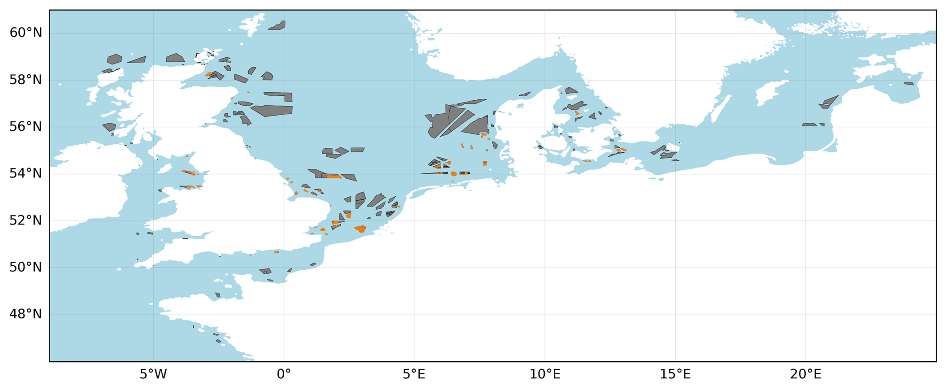
Figure A1 Depiction of the raw EMODnet wind farm polygon data: Polygons labeled as “Production” (existing farms) are highlighted in orange while polygons labeled as “Approved”, “Constructed”, “Planned” or “Dismantled” are displayed in gray.

The following wind farms in the EMODnet database have been merged to a single polygon by aggregating installed capacity, area, and number of turbines:

• (Belgium) Borssele Kavel III and Borssele Kavel IV to Borssele III + IV

• (Belgium) C-Power¹ (Zone A) and C-Power (Zone B) to C-Power

• (Belgium) Belwind phase 2 (Nobelwind) (Zone 2) and Belwind phase 2 (Nobelwind) (Zone 1) to Belwind phase 2

• (United Kingdom) Robin Rigg East and Robin Rigg West to Robin Rigg

• (United Kingdom) Hornsea Project 1 (Heron East) Wind Farm, Hornsea Project 1 (Heron West) Wind Farm and Hornsea Project 1 (Njord) Wind Farm to Hornsea Project 1

• (United Kingdom) Walney Extension 3 and Walney Extension 4 to Walney Extension

The following polygons were removed because of redundancy within EMODnet itself

• (Belgium) Borssele

The following wind farms level information in EWFD were merged to a single farm by aggregating installed capacity, area, and number of turbines:

• (Belgium) three entries related to Thorntonbank

• (United Kingdom) Greater Gabbard Extension and Greater Gabbard 2

• (United Kingdom) two entries related to Walney Extension

• (United Kingdom) Hornsea Project One - Heron Wind and Hornsea Project One – Njord

For more details, the reader is referred to the code base repository (Imberger et al., 2025).

A3 Representativeness of the selected simulation period

We used the open-source CLIMatological REPresentative PERiods (CLIMREPPER) software package (DTU Wind, 2025) to assess the representativeness of the chosen periods. CLIMREPPER “provides algorithms for the determination of climatological representative periods for statistical-dynamical downscaling applications or for general quantification of the climatological representativeness of a period of interest” (DTU Wind, 2025). It stems from existing studies (Technical University of Denmark and Max-Planck-Institute, 2020; Fischereit et al., 2022c, b) and has now been remodeled, generalized to use ERA5 data, and made open source.

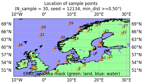
Figure A2 Sample locations used to derive the representativeness of the 2 months selected.

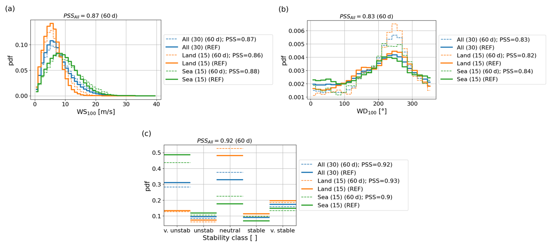
Figure A3 Probability density functions (pdf) for (a) wind speed at 100 m (WS₁₀₀), (b) wind direction at 100 m (WD₁₀₀) and (c) stability class for (dashed lines) February 2020 and August 2022 combined (60 d) and for (solid bold lines) 1994–2023 climatic average (REF) for (orange) mean over 30 different locations (Fig. A2) and (green) land locations and (blue) water locations based on the ERA5 land-mask value of 0.5. PSS is the Perkins skill score (Eq. A1.)

Two months were selected for this study: February 2020 and August 2022. These 2 months were selected to capture both winter and summer conditions. To evaluate their representativeness for the climate of the NEA domain, 30 sample points within the domain were randomly selected (Fig. A2). For each sample point, the 30-year (1994–2023) binned climatological probability density function (pdf) Z^c(i) with bins i were calculated for the 100 m wind speed (WS₁₀₀) and wind direction (WD₁₀₀), and the stability from ERA5 (Hersbach et al., 2018). Stability is calculated by deriving the Monin–Obukhov length from ERA5 according to ECMWF (2024) and then applying the stability categories as presented in Holtslag et al. (2014). Then the same binned pdfs are calculated for the two sample months (February 2020 and August 2022, $Z_{N\left(t\right)=\mathrm{02.2020}+\mathrm{08.2022}}^{\mathrm{s}}\left(i\right)$).

Figure A3 shows both the climatological pdfs (solid bold line) and the pdfs of the 2 months (dashed line) for the three variables (a) WS₁₀₀, (b) WD₁₀₀, and (c) stability class. The pdfs of the 2 months compare well with the climatological pdfs, especially for wind speed. This is confirmed by the Perkins skill score (PSS, Perkins et al., 2007). As described in Fischereit et al. (2022c), the PSS evaluates how well two discrete pdfs, Z^c(i) and $Z_{N\left(t\right)}^{\mathrm{s}}\left(i\right)$, overlap for each bin i:

$$\begin{array}{}\text{(A1)}& \text{PSS}(l,t)=\sum _{i=\mathrm{1}}^{n}min\left[Z^{\mathrm{c}}(i,l),Z_{N\left(t\right)}^{\mathrm{s}}(i,t,l)\right].\end{array}$$

where Z^c(i,l) is the discrete daily climatological pdf at a certain location l for all hourly sample times T, i.e. $Z^{\mathrm{c}}(i,l)=Z_T^{\mathrm{s}}(i,l)=Z^{\mathrm{s}}(i,T,l)$. $Z_{N\left(t\right)}^{\mathrm{s}}(i,t,l)$ is the daily sample pdf for a certain number of sample days N made up of t days within T. The value of PSS is close to zero for almost no overlap of the two pdfs and approaches one for a perfect match. According to Perkins et al. (2007), a good agreement between two pdfs can be defined for PSS>0.8 and a near-perfect agreement for PSS>0.9. The PSS for wind speed (0.87), wind direction (0.83), and stability (0.92) confirm that the 2 months are relatively well suited to represent the 30-year climate, although they are not a perfect match. Overall, slightly higher wind speeds, more westerly wind directions, and more neutral and less very unstable and very stable situations are included in the 2 months compared to the 30-year average.

Figure A4 As Fig. A3, but only for February 2020 (29 d).

Figure A5 As Fig. A3, but only for August 2022 (31 d).

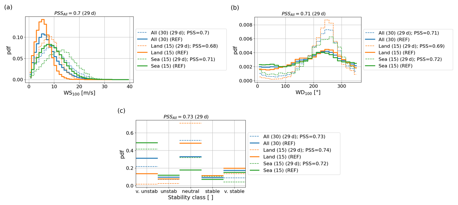
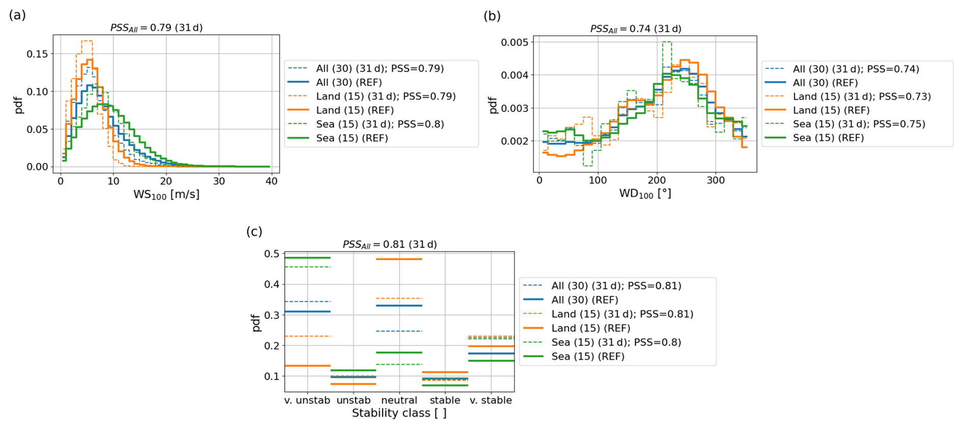
Similar plots for the 2 months separately (Fig. A4 and A5) show that in February 2020, winds were much stronger, more westerly, and the atmosphere more neutrally stratified compared to the climatological average. On the contrary, August 2022 had weaker winds and more very stable and very unstable conditions than the climatological average. Therefore, putting the 2 months together resulted in conditions similar to the 30-year average.

A4 Monthly averages

In this section, we show the monthly averages for wind speed at a height of 100 m in February 2020 (Fig. A6) and in August 2022 (Fig. A7) separately.

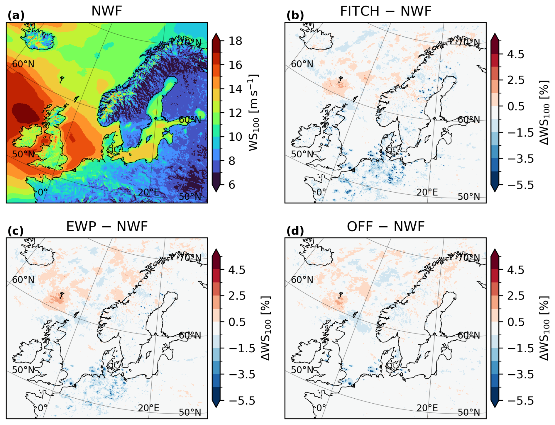
Figure A6 Same as Fig. 14, but only for February 2020.

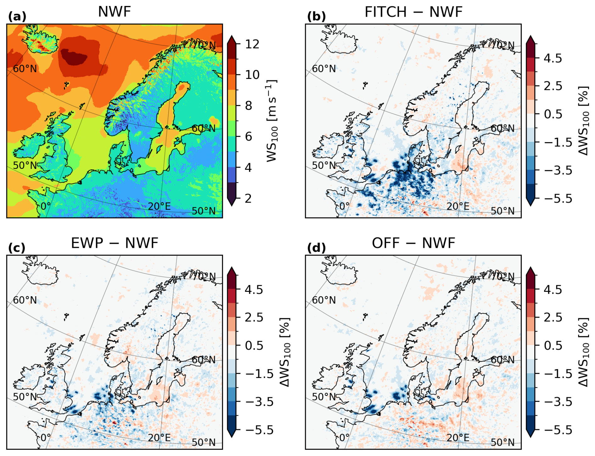
Figure A7 Same as Fig. 14, but only for August 2022.

A5 Applied significance test for spatially and temporally autocorrelated data

Standard significance tests, like Student's t-test, cannot be applied to spatially and temporally autocorrelated data and with an unknown underlying distribution. Thus, we use the significance test suggested by Wilks (1997) and Marchand et al. (2006). We describe the method in brief in the following, following Marchand et al. (2006) closely.

The main goal of these tests is to check whether two sets Y and Z of length n_y and n_z have the same distributions, i.e., if they come from a common parent distribution and thus are not statistically significantly different. First, the two sets are combined into a single set $\mathit{X}=\mathit{Y}\cup \mathit{Z}$ and the true population distribution is approximated by a large number n_b of bootstrap re-samples Y^∗ and Z^∗ with replacement from that combined set. The length of the two bootstrap resamples corresponds to the length of each set (n_y and n_z, respectively). Based on the normalized standard difference between the two bootstrap resamples, a distribution of the test statistic can be calculated as it produces n_b values of d^∗:

$$\begin{array}{}\text{(A2)}& d^{\ast }={\displaystyle \frac{\stackrel{\mathrm{‾}}{z}-\stackrel{\mathrm{‾}}{y}}{\stackrel{\mathrm{‾}}{\mathit{\sigma }}\sqrt{\mathrm{1}/n_z+\mathrm{1}/n_y}}}\end{array}$$

with $\stackrel{\mathrm{‾}}{z}-\stackrel{\mathrm{‾}}{y}$ being the difference of the means between Y^∗ and Z^∗ and the estimated standard deviation

$$\begin{array}{}\text{(A3)}& \stackrel{\mathrm{‾}}{\mathit{\sigma }}={\left({\displaystyle \frac{{\sum }_{i=\mathrm{1}}^{n_z}(z_i-\stackrel{\mathrm{‾}}{z}{)}^{\mathrm{2}}+{\sum }_{j=\mathrm{1}}^{n_y}(y_j-\stackrel{\mathrm{‾}}{y}{)}^{\mathrm{2}}}{n_z+n_y-\mathrm{2}}}\right)}^{\mathrm{1}/\mathrm{2}}\end{array}$$

The same test statistic d can be calculated from the original sample sets Y and Z. Since d^∗ is a distribution, we can determine if d falls inside or outside of the confidence interval of the d^∗. If it falls outside, we can reject the null hypothesis that the two sets come from a common parent distribution. Here we use the 90-percentile confidence interval.

To account for the temporal correlation within this time series Wilks (1997) developed a “moving blocks” bootstrap resampling technique. The idea is to derive a characteristic block length L for each grid point. Then, random samples x_i are selected from Z and a block of length L is taken with replacement from Z containing x_i. This process is repeated until the new sample is the same length as the original sample of Y. The final problem is to determine the size of the block length L. It has “to be large enough to capture the temporal correlation structure of the time series data. If too small a block length is used, the bootstrap blocks are treated as being independently sampled when in fact they are not, leading to the bootstrap underestimating the variability in the distribution of the d^∗ statistic” (Marchand et al., 2006). Here we follow Wilks (1997) method for first-order autoregressive [AR(1)] processes and determine the block-length iteratively using the lag+1 autocorrelation.

A6 Daytime temperature average

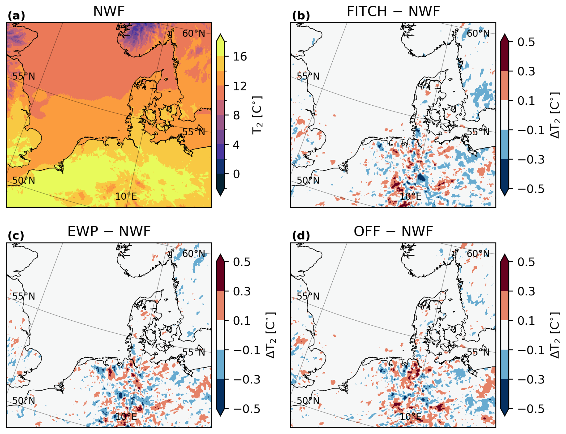
Figure A8 As Fig. 18, but averaged during daytime (12:00–16:00 UTC) conditions only.