SDMBCv2 (v1.0): correcting systematic biases in RCM inputs for future projection

Regional Climate Models (RCMs) offer enhanced spatial resolution and a more realistic depiction of local climate processes. However, they often inherit systematic biases from their driving Global Climate Models (GCMs), which can compromise the accuracy of downscaled climate projections. To address this, bias correction techniques have been widely employed to adjust GCM and RCM outputs, particularly for climate impact and adaptation studies. Traditional methods, however, typically correct surface variables independently and lack physical and dynamical consistency. Bias correcting GCM boundary conditions prior to RCM simulation ensures a more coherent, physically and dynamically consistent, regional climate simulation with reduced errors. This study evaluates the effectiveness of such an approach using a calibration/validation framework, demonstrating significant error reduction during the validation (out-of-sample) period compared to uncorrected GCM data. We present an updated version of the open-source Python package, Sub-Daily Multivariate Bias Correction (SDMBC) v2, designed to correct RCM input variables using both reanalysis and raw GCM datasets. Enhancements include support for future climate projections, flexible horizontal and vertical interpolation for compatibility with diverse datasets, and a fully Python-based architecture optimized for parallel processing and high-performance computing. This paper illustrates the software's capabilities and provides a practical application example.

1 Introduction

The growing need to address the limitations of Global Climate Models (GCMs) in regional and hydrological contexts has led to the widespread use of downscaling approaches. These methods refine coarse-resolution GCM outputs into finer resolutions suitable for regional applications, such as water resource management and climate change adaptation. Dynamical downscaling employs Regional Climate Models (RCMs) with boundary conditions derived from GCMs, offering a more realistic representation of local physical processes that influence variables such as near-surface air temperature and precipitation. The enhanced resolution provided by RCMs aids in designing new infrastructure standards, assessing water vulnerability, evaluating drought risk, and gaining crucial insights into human health risks.

Despite the advantages of RCMs, they inherit biases from the driving GCMs, resulting in significant errors and artifacts that can diminish the benefits of dynamical downscaling (Rocheta et al., 2017; Kim et al., 2021; Risser et al., 2024). The propagation of GCM biases into RCM outputs through the RCM input boundaries raises concerns about the fidelity and reliability of future climate projections. To address this issue, bias correction techniques have been developed and widely applied.

In the context of dynamical downscaling, bias correction can be implemented either before or after running the RCM. Post-downscaling bias correction can be applied to the variables of interest to climate data users, such as surface air temperature and precipitation. This approach builds a model that closely represents the observed climate using statistical relationships between reanalysis and simulations. It remains a widely used approach due to its relatively simple bias correction process and low computational cost (Mehrotra and Sharma, 2015; Cannon, 2018; Tabari et al., 2021). In line with these attempts, to simplify this process, various software toolkits have been developed. Cannon (2016) developed an R package supporting multiple bias correction techniques, from simple quantile mapping to advanced methods that correct multivariate relationships between surface variables. Mehrotra et al. (2018) developed an R package that supports bias correction approaches for multiple surface variables across different time scales, focusing on low-frequency precipitation variability using a nested approach. While these packages simplify the bias correction process, enabling users to easily correct variables and analyze model performance, they can present challenges due to artifacts in downscaled signals and assumptions of time invariance when correcting output variables directly (Rahimi et al., 2024).

Pre-downscaling bias correction, on the other hand, involves adjusting the GCM's climatological statistics towards reanalysis data to remove biases from the GCM datasets. Several approaches for bias correction have been employed, ranging from simple scaling (Xu and Yang, 2012; Bruyere et al., 2014) to more complex techniques that attempt to mimic observed multi-scale relationships in simulations (Rocheta et al., 2017; Kim et al., 2021, 2023a). These methods correct RCM input boundary conditions and have been shown to improve the accuracy of output variables, particularly for extreme events (Kim et al., 2023a). Furthermore, Kim et al. (2023b) demonstrated that multivariate bias-corrected boundary conditions better represent compound events where multiple extremes occur simultaneously at the same location. Although this approach, while effective, may disrupt the physical consistency between variables in the GCM boundary conditions when correcting statistics of the simulated variables toward those of reanalysis data, the RCM will re-establish its own internal relationships between variables in the downscaled outputs, which are physically consistent and interpretable (Rahimi et al., 2024).

A recent study developed a multivariate bias correction approach at the sub-daily time scale to correct the rainfall diurnal cycle, which is crucial for simulating extreme events. They used quantile mapping (QM) to adjust the probability distribution of the scale factor, highlighting that sub-daily correction of the RCM input boundary conditions can improve diurnal precipitation patterns and other statistics compared with daily correction (Kim et al., 2023c).

In brief, pre-downscaling bias correction shows improved performance, particularly for extreme events, while ensuring the physical and dynamical consistency of RCM outputs. Despite these advantages, this bias correction process requires large matrices and complex mathematical formulations, making it challenging for users to apply and limiting the benefits of correcting atmospheric variables before downscaling. To resolve this issue, a previous study developed a Python package that corrects full atmospheric fields at a sub-daily time scale before generating RCM input boundary conditions, focusing on the historical period (Kim et al., 2023d). However, it was limited in application due to its Fortran-based script with inefficient data handling in the previous implementation, resulting in high memory usage when processing large datasets, and a fixed input format, which needs pre-processing that requires users to have fairly advanced programming skills.

This study focuses on the sub-daily multivariate bias correction of GCM simulations before dynamical downscaling to address these issues, making the software applicable to most GCMs for simulating future climate and maximizing the capabilities of bias correction.

This study developed a Python package, Sub-Daily Multivariate Bias Correction (SDMBC) v2, for future projections, which corrects the full atmospheric fields and sea surface temperature of GCM datasets for both historical and future climate. It supports high-performance computing, enabling parallel and efficient bias correction using several recently published packages. It includes several bias correction approaches at multiple time scales, from sub-daily to seasonal. The package is primarily written in Python for efficiency in processing multiple input files, with the core bias correction process remaining in Fortran due to its superior numerical calculation capabilities. The Fortran subroutines are compiled into a Python-accessible module via F2PY, included with NumPy, facilitating efficient interaction between Fortran and Python.

This paper describes the updated software package that simplifies the bias correction process. The paper is organized as follows: Sect. 2 describes the bias correction approaches, Sect. 3 provides general details of implementing the bias correction method in the Python package, Sect. 4 presents the experiment design, Sect. 5 presents the results, and Sect. 6 concludes the study.

2 Bias correction approaches

A recent study developed a sub-daily multivariate bias correction approach to address the limitation of RCMs in reproducing observed sub-daily rainfall intensities, particularly the diurnal cycle of precipitation (Kim et al., 2023c). This approach combines QM and a multivariate bias correction method to adjust biases in the distributions at a sub-daily time scale, as well as the inter-variable relationships among atmospheric variables at multiple time scales before dynamical downscaling, aiming to enhance the simulation of extreme events and the diurnal precipitation cycle within the RCM domain. Users can define the statistical attributes that should be corrected from: mean, standard deviation, and dependence attributes, lag1 auto-, and lag0 cross-correlation. The input variables are corrected at multiple time scales using a nesting approach, and the bias correction processes are repeated a predefined number of times. The nesting approach, which corrects temporal persistence as a form of the weighting factors, has shown improvement in the simulation of extreme events (Johnson and Sharma, 2012), and a total number of iterations has been set to one as a default to avoid overcorrecting that can occur during the bias correction process (Mehrotra and Sharma, 2012). More information on this approach can be found in Kim et al. (2023c). To evaluate the bias correction techniques employed in this study, two time periods were selected. For calibration, a 31-year sample spanning from 1959 to 1989 was chosen from both the GCM and observed data to compute the bias correction factors. These factors were then applied to data from a separate period for validation, 1990 to 2020, to assess whether the bias correction performs effectively when applied outside the calibration sample.

Figure 1 A schematic diagram of SDMBCv2.

3 Bias correction of historical and future simulation package, SDMBCv2

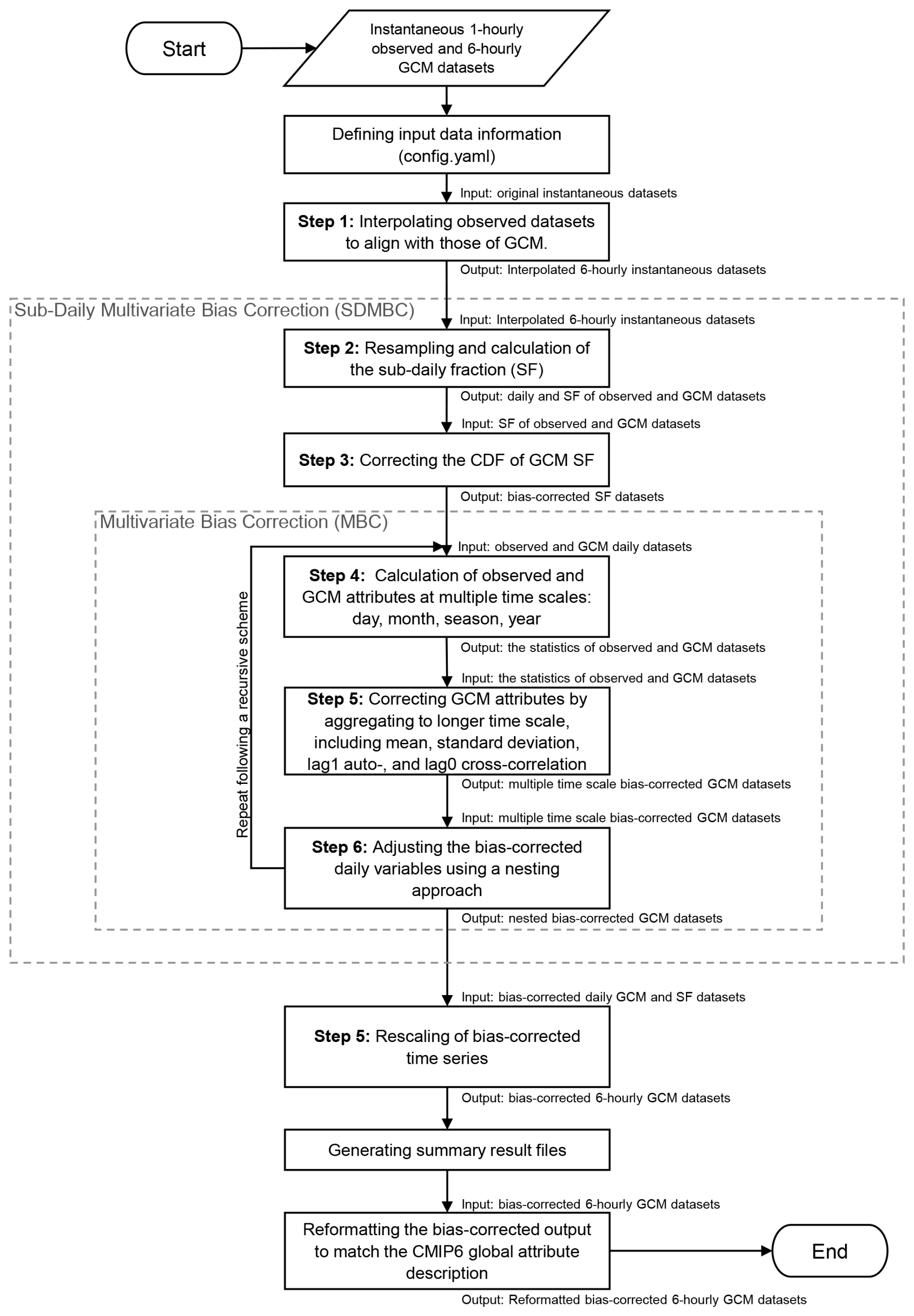
The SDMBCv2 developed here represents the next generation of SDMBC, providing bias-corrected atmospheric variables for both future and historical periods. This section outlines the application of bias correction methods to the instantaneous input datasets, encompassing interpolation and reformation (see Fig. 1). It details the input requirements, interpolation processes, implementation of bias corrections, and the output formats available in the package.

3.1 User-defined input information for interpolation

Before applying bias correction, users first need to interpolate the reanalysis dataset to match the spatial and temporal resolution of the target GCM. This preprocessing step ensures that both datasets share a consistent grid structure, facilitating seamless integration. The software developed in this study automates this process through horizontal and vertical interpolation, with input and output specifications managed via a configuration file (“config_interp.yaml”).

The interpolation procedure involves resampling key atmospheric variables – including specific humidity (q, kg kg⁻¹), temperature (t, K), zonal wind (u, m s⁻¹), meridional wind (v, m s⁻¹), and sea surface temperature (sst), which define the lateral and lower boundary conditions of the model. Here, 6-hourly instantaneous values are used.

For horizontal interpolation, the software employs bilinear or conservative remapping techniques, depending on the variable, utilizing the xESMF library and Climate Data Operators (CDO) for high-precision grid transformations. Vertical interpolation is performed by aligning the input dataset's coordinate system with the target model's levels, incorporating geopotential height information to ensure consistency. To optimize performance and scalability, the script is designed to handle large datasets efficiently using Dask for parallel processing. This implementation enhances computational efficiency while maintaining accuracy, ensuring the interpolated reanalysis datasets are well aligned with the GCM for subsequent bias correction and climate simulations.

Interpolation is necessary for the reanalysis dataset during both calibration and validation periods to enable proper bias correction functioning.

3.2 Overview of bias correction for a historical period

Once the input datasets have been accurately interpolated, the next step involves applying bias correction to the GCM variables. This process ensures that the climatological statistics of the GCM data are aligned with those of the reanalysis dataset, improving the reliability of the corrected outputs. The bias correction procedure consists of multiple key steps and follows an approach similar to that implemented in the SDMBC package. A concise overview of this methodology is provided in the following section, with further technical details available in the SDMBC documentation and Kim et al. (2023d).

3.2.1 Reanalysis and GCM attributes calculation

Prior to bias correction, both reanalysis and GCM 6-hourly instantaneous datasets are aggregated to a daily time scale by computing the mean of the 6-hourly values. During this process, sub-daily fractions (SF), representing the contribution of each 6 h value to the daily average, are calculated and stored for subsequent use in downscaling bias-corrected daily variables back to their original 6-hourly resolution. The software includes a QM approach to correct scaling factors, adjusting the distribution of GCM outputs to align with the cumulative distribution function (CDF) of the reanalysis. Users can specify the use of sub-daily bias correction in the configuration file, enabling this adjustment process.

Key statistical attributes are computed using a centered moving window approach (Sharma and Lall, 1999) for both observed and GCM variables using the resampled daily time series. A detailed description of the transformation function applied in this study is provided in Kim et al. (2023c).

3.2.2 Correction of GCM attributes

To correct the raw daily GCM variables, we first adjust their climatological mean and standard deviation. This is achieved by replacing the GCM mean with the reanalysis mean, then normalizing by the GCM standard deviation and rescaling with the reanalysis standard deviation. The transformed time series are subsequently standardized, after which adjustments are applied to preserve both auto- and cross-correlation structures using a simplified multivariate autoregressive model (Salas, 1980).

Following these adjustments, the bias-corrected daily series are aggregated to longer temporal scales, including monthly and seasonal periods. The corrected values are then rescaled to maintain consistency in mean and standard deviation. Additionally, the bias-corrected variables are integrated into a hierarchical nesting framework (Kim et al., 2023a), where daily GCM data incorporate bias correction effects observed at coarser temporal scales. This approach ensures that persistence characteristics are retained across time scales. The bias-corrected values at multiple time scales serve as weighting factors for the uncorrected daily GCM data, as outlined by Srikanthan and Pegram (2009). These bias correction steps are iteratively applied in a recursive manner, with the total number of iterations defined by the user. In this study, we perform one iteration, as noted in Sect. 2.

Finally, the bias-corrected daily series are rescaled to a 6-hourly resolution using the sub-daily fractions calculated previously. A detailed description of these procedures is provided in Fig. 1.

3.3 Overview of bias correction for a future projection

The next step involves applying bias correction parameters to future GCM variables. This process aims to align the climatological statistics of the future GCM data with those of the differences between GCM and reanalysis in the current period. The following sections provide an overview of the bias correction methodology applied to future GCM data, with further details available in the relevant documentation.

3.3.1 Calculation of future GCM attributes

Future GCM 6-hourly instantaneous datasets are first aggregated to a daily time scale by averaging the 6-hourly values, following the same approach used for historical data. Users can enable sub-daily bias correction for future periods through the configuration file, allowing for refined adjustments. Key statistical attributes – including climatological mean, standard deviation, lag-1 auto-correlation, and lag-0 cross-correlation – are then computed for future GCM variables across multiple time scales, ranging from daily to seasonal periods.

3.3.2 Correction of future GCM attributes

Bias correction parameters derived from the historical period are applied to future simulations. For sub-daily correction, the same QM approach used for historical data is implemented. This involves determining the difference between the CDFs of reanalysis and current-climate GCM data and using this difference to correct future GCM values under the assumption that biases present in the current period will persist in future simulations. The correction process begins by correcting the future GCM climatological mean, achieved by subtracting the difference between the current GCM and reanalysis climatological means. The standard deviation is then corrected by scaling it according to the ratio of the reanalysis standard deviation to the current GCM standard deviation. Additionally, auto- and cross-correlation coefficients are adjusted to preserve observed dependencies within nested and multivariate bias correction frameworks. The bias correction parameters derived from historical periods can be applied recursively, with the total number of iterations defined by users. Further details on these procedures are available in Kim et al. (2023d).

3.4 Output data information

The bias-corrected GCM datasets used for generating RCM input boundaries include four three-dimensional atmospheric variables at each vertical level, along with sea surface temperature. The package allows these outputs to be automatically reformatted to match the original file structure, provided users specify this option in the configuration file. As a result, the bias-corrected outputs retain the same NetCDF format as the original GCM data, simplifying the integration into existing RCM workflows. This ensures seamless integration into RCM workflows, allowing users to employ the same scripts or procedures previously used with raw GCM inputs.

4 Experiment design

This section presents the datasets and experimental design employed in the study, as well as the evaluation metrics used.

4.1 Datasets and experimental setup

To evaluate the performance of SDMBCv2, we used the Australian Community Climate and Earth System Simulator Earth System Model Version 1.5 (ACCESS-ESM1.5) (Ziehn et al., 2020) as the source GCM. ACCESS-ESM1.5 operates on an N96 Gaussian grid with a spatial resolution of approximately 1.875° longitude × 1.25° latitude and includes 38 vertical levels. ERA5, the fifth-generation reanalysis dataset from the European Centre for Medium-Range Weather Forecasts (Hersbach et al., 2020), was used as the reference. It provides a horizontal resolution of approximately 31 km and includes 37 pressure levels.

Bias correction was applied to key variables required for regional climate model boundary conditions: specific humidity q (kg kg⁻¹), temperature ta (K), zonal wind u (m s⁻¹), and meridional wind v (m s⁻¹), and sea surface temperature sst (K).

The SDMBCv2 package first harmonized the spatial and temporal resolutions between the GCM and ERA5 datasets through a two-step interpolation process: conservative remapping was used for specific humidity to ensure moisture mass conservation, while bilinear interpolation was applied to the remaining variables. Vertical interpolation was performed to align the ERA5 levels with the vertical structure of ACCESS-ESM1.5. SST regridding was also necessary to ensure consistency with the GCM grid.

Both datasets were preprocessed to ensure identical spatiotemporal dimensions prior to bias correction. This alignment ensures that corrected GCM variables can be seamlessly used as input boundary conditions for regional climate models. It is important to note that all other model variables remain unchanged and that boundary conditions are established only after bias correction is applied.

The bias correction process was conducted over two distinct periods: 1959–1989 (calibration) and 1990–2020 (validation), with 31-year periods selected to allow one year for spin-up in downscaling applications, resulting in a 30-year climatology.

4.2 Performance assessment

The impact of bias correction was evaluated using two primary statistical metrics: Mean Absolute Error (MAE) and Bias. The MAE quantifies the average absolute difference between model simulations and observed values across all grid cells and is defined as:

$$\begin{array}{}\text{(1)}& \text{MAE}={\displaystyle \frac{\mathrm{1}}{N}}\sum _{n=\mathrm{1}}^N\left|X_n^{\text{mod}}-X_n^{\text{obs}}\right|,\end{array}$$

where N is the total number of grid cells, $X_n^{\text{mod}}$ and $X_n^{\text{obs}}$ represent the climatological values from the GCM and reanalysis at each grid cell, respectively.

Bias, representing the systematic deviation between model simulations and reanalysis, is calculated as:

$$\begin{array}{}\text{(2)}& \text{Bias}={\displaystyle \frac{\mathrm{1}}{N}}\sum _{n=\mathrm{1}}^N\left(X_n^{\text{mod}}-X_n^{\text{obs}}\right).\end{array}$$

Bias values are computed individually for each grid cell.

Additionally, the Kolmogorov-Smirnov (K–S) test was employed to statistically evaluate the similarity between the probability distributions of model simulations and reanalysis. The K–S test measures the maximum absolute difference (L) between the cumulative distribution functions (CDFs) of the model (F_g(x)) and observed (F_o(x)) data:

$$\begin{array}{}\text{(3)}& L=\left|F_{\mathrm{g}}\left(x\right)-F_{\mathrm{o}}\left(x\right)\right|.\end{array}$$

The null hypothesis of the K–S test is that both samples originate from populations with identical distributions. The null hypothesis is rejected if the calculated test statistic (L) exceeds the critical value ($L_{\text{critical}}=c\left(\mathit{\alpha }\right)\sqrt{\frac{n_{\mathrm{1}}+n_{\mathrm{2}}}{n_{\mathrm{1}}{n}_{\mathrm{2}}}}$), where n₁ and n₂ denote the sample sizes of the model and reanalysis, respectively, and c(α) is a constant determined by the significance level α. Alternatively, rejection occurs if the p-value is less than 0.05.

5 Results

This section presents an evaluation of the bias correction performance across multiple time scales. We assess the correction performance by comparing key climatological statistics during both the calibration and validation periods against reanalysis datasets. Although the SDMBCv2 package produces bias-corrected outputs across full vertical levels and spatial domains, this study focuses on selected grid cells for vertical analysis and lower atmospheric levels for horizontal. The evaluation is based on several diagnostic metrics, including the climatological mean, standard deviation, lag-1 autocorrelation, multivariate dependence, and sub-daily distribution characteristics.

5.1 Bias-corrected GCM datasets: calibration

This section assesses the performance of the bias correction during the calibration period. The primary goal is to evaluate whether the SDMBCv2 framework reduces biases in key statistical properties across various time scales.

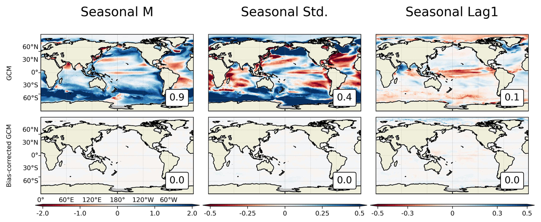
Figure 2 Seasonal bias map of sea surface temperature (SST) for both GCM and bias-corrected data in calibration periods from 1959 to 1989. The number at the bottom right shows the mean absolute error.

Figure 2 presents bias maps of the seasonal statistics used to evaluate seasonal variability in SST, where seasonal-scale diagnostics highlight the dominant systematic biases, comparing uncorrected and bias-corrected GCM outputs against ERA5 for the calibration period. The upper panels display the biases in the raw GCM, while the lower panels illustrate the results after bias correction with SDMBCv2.

The raw GCM exhibits a strong negative bias in the seasonal mean, particularly in the Southern Ocean, with a domain-averaged mean absolute bias of 0.9 °C. The standard deviation is also notably overestimated in several key regions, including the tropical Atlantic and Pacific, with an average bias of 0.4 °C. Biases in lag-1 autocorrelation are generally lower in magnitude but still evident in convectively active regions, with localized deviations exceeding 0.3. Such errors can influence the representation of SST persistence and feedback in coupled models.

In contrast, the bias-corrected SST fields show near-zero deviations across all three metrics indicating good agreement with the reference.

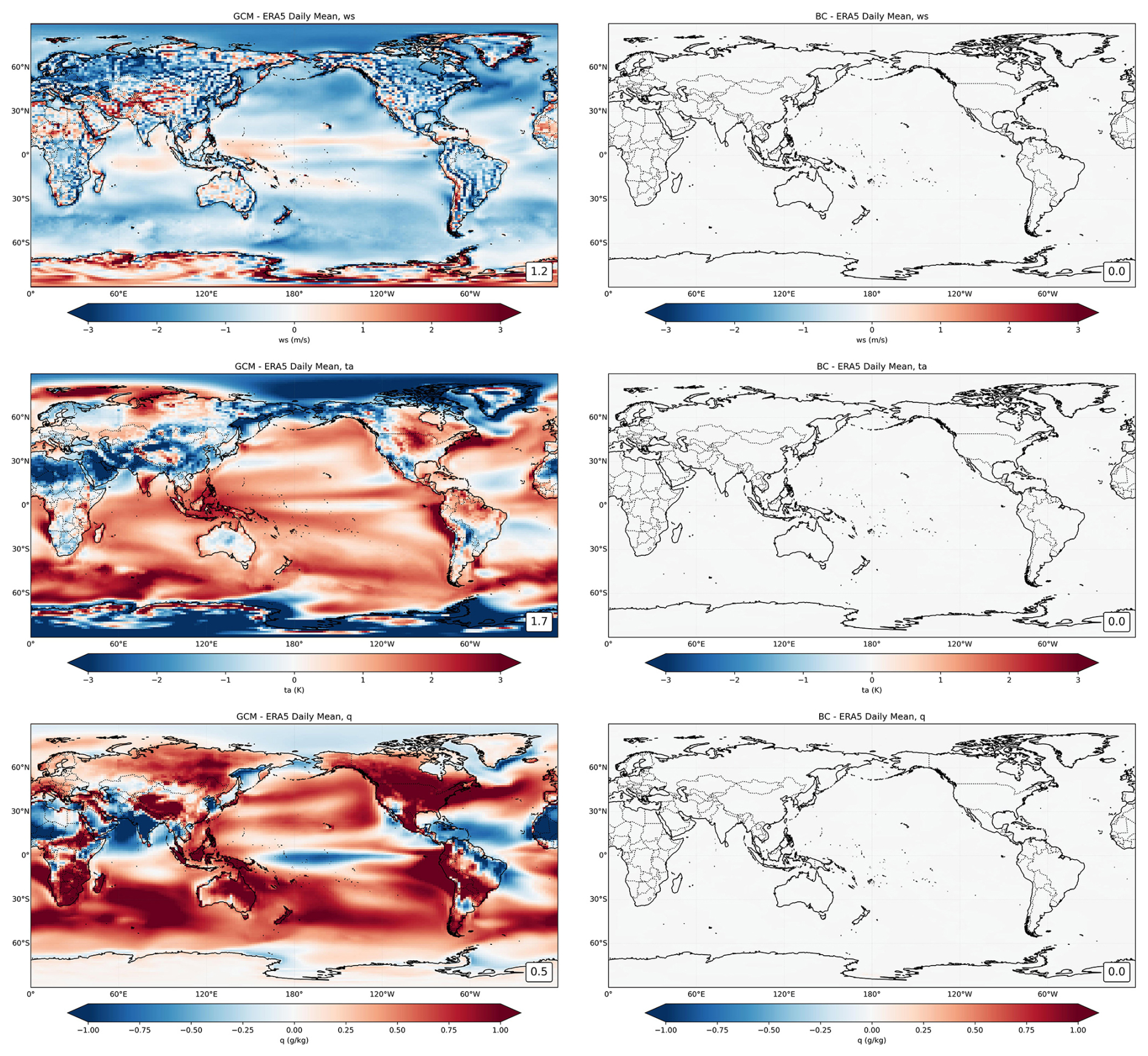
Figure 3 Climatological mean bias maps comparing ERA5 with GCM outputs before (left panels) and after (right panels) bias correction (BC), evaluated at the lowest model level on a daily time scale for the calibration period (1959–1989). The panels show results for wind speed (ws), air temperature (ta), and specific humidity (q). The number at the bottom right shows the mean absolute error.

Figure 3 presents bias maps of the climatological mean, comparing ERA5 to both the uncorrected and bias-corrected GCM outputs for three atmospheric variables at the lowest model level on a daily time scale across the entire domain.

The left panels reveal substantial biases in the original GCM outputs, including an obvious underestimation of wind speed, widespread warm biases in air temperature, and excessive specific humidity, particularly across the tropics and mid-latitudes. These systematic errors can propagate through regional climate models, degrading their performance. For instance, underestimated wind speed may suppress key processes like moisture transport and convective uplift, while overestimated temperature and humidity can amplify convective feedback, potentially distorting projections of extreme events such as heatwaves or intense precipitation.

In contrast, the right panels demonstrate the effectiveness of SDMBCv2 in eliminating these biases. The post-correction fields show negligible residual errors across all three variables.

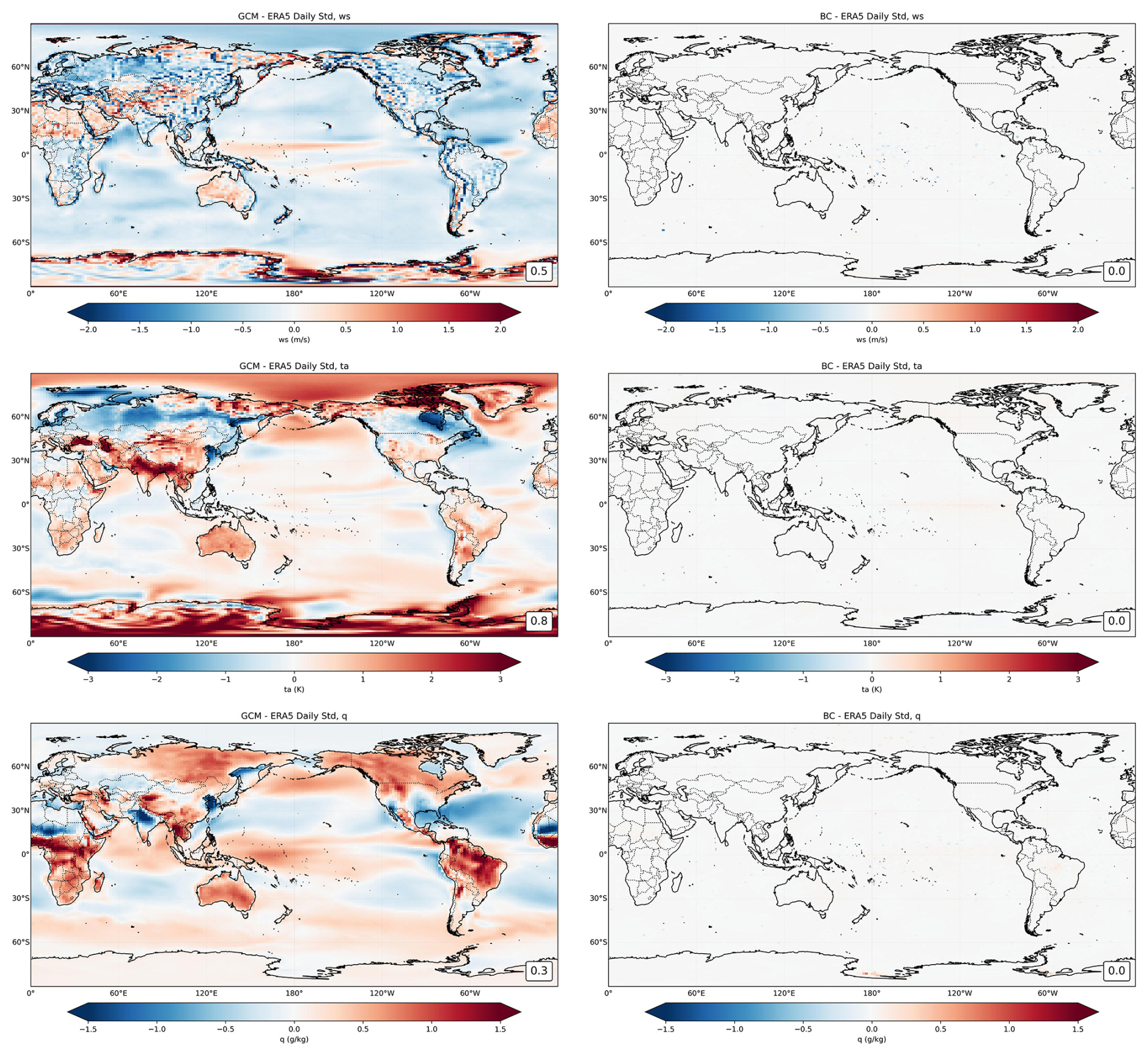
Figure 4 As in Fig. 3, but for standard deviation.

Figure 4 presents bias maps of the standard deviation, corresponding to the climatological mean comparisons shown in Fig. 3. These maps illustrate how the SDMBC framework improves the representation of daily variability in key atmospheric variables. The results show that the uncorrected GCM exhibits notable deficiencies. Wind speed variability is underestimated, particularly across mid-latitude regions, potentially suppressing the simulation of wind-driven processes such as turbulence, vertical mixing, and mesoscale circulation. Specific humidity also shows strong positive biases in the tropics, indicating an overrepresentation of moisture variability. Such biases can exaggerate convective activity and lead to unrealistic intensification of extreme rainfall events in downscaling applications. On the other hand, biases in variability are substantially reduced after bias correction across most regions, with near-zero deviations in wind speed, temperature, and specific humidity.

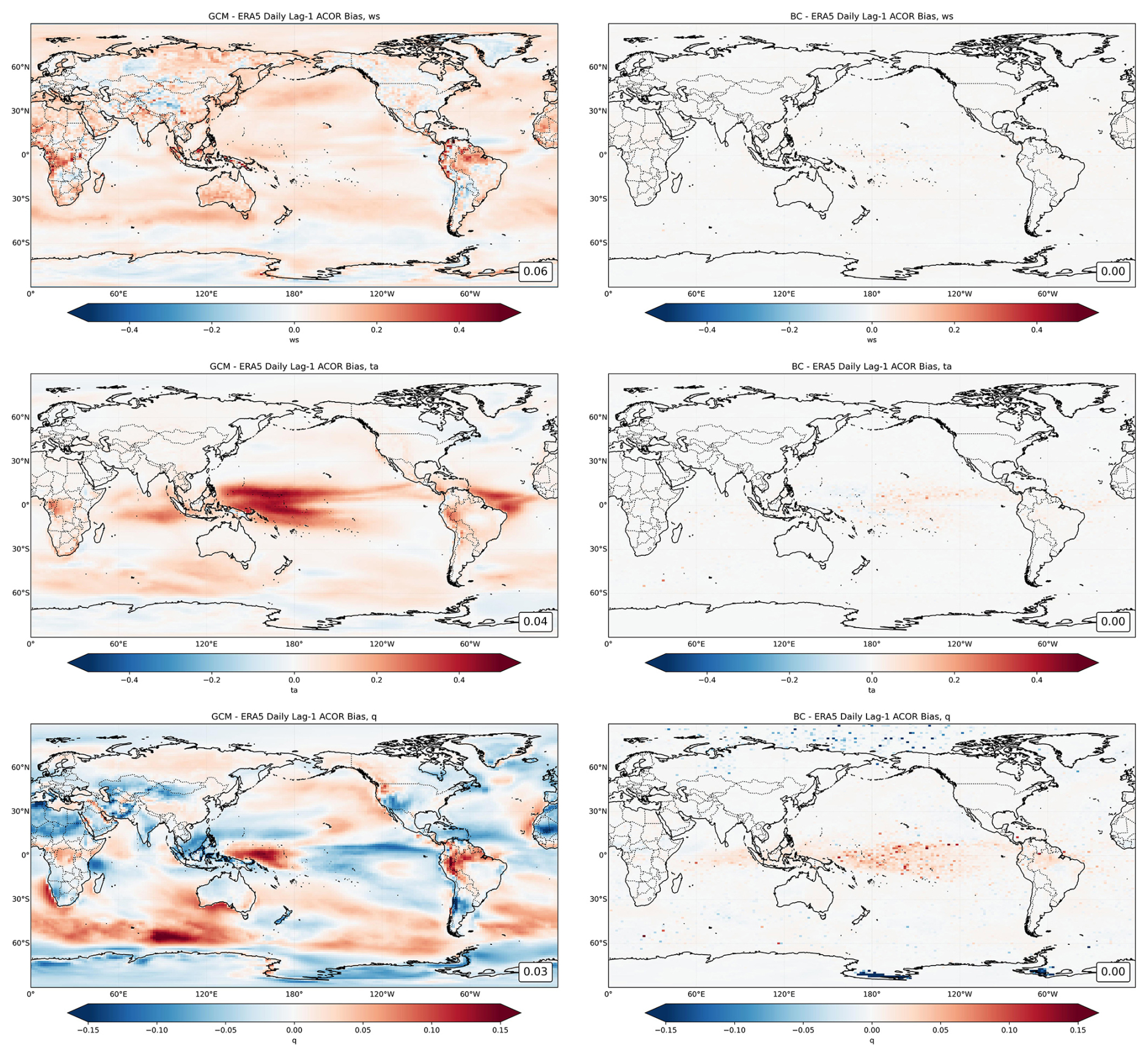
Figure 5 As in Fig. 3, but for lag1 auto-correlation. Domain-averaged MAE values are shown; very small errors (∼ 10⁻³) appear as 0.00 due to rounding.

Figure 5 compares lag-1 autocorrelation between the uncorrected GCM and the bias-corrected GCM at a daily timescale. The results indicate that the uncorrected GCM displays widespread positive biases in lag-1 autocorrelation, especially for air temperature over tropical regions and for specific humidity in convective zones. These positive biases indicate that the model overestimates short-term memory, potentially leading to an unrealistic persistence of extreme events such as prolonged heatwaves or wet spells. Conversely, positive biases in wind speed autocorrelation are also evident, suggesting that the model overrepresents the continuity of wind motion, which could influence the simulation of storms and large-scale circulation features.

Following bias correction, these spurious persistence patterns are largely removed. The corrected fields show near-zero biases across most regions, indicating that SDMBCv2 successfully adjusts not only the mean and variability but also the temporal correlation structure of atmospheric variables – an essential feature for improving the realism of climate simulations used in downscaling.

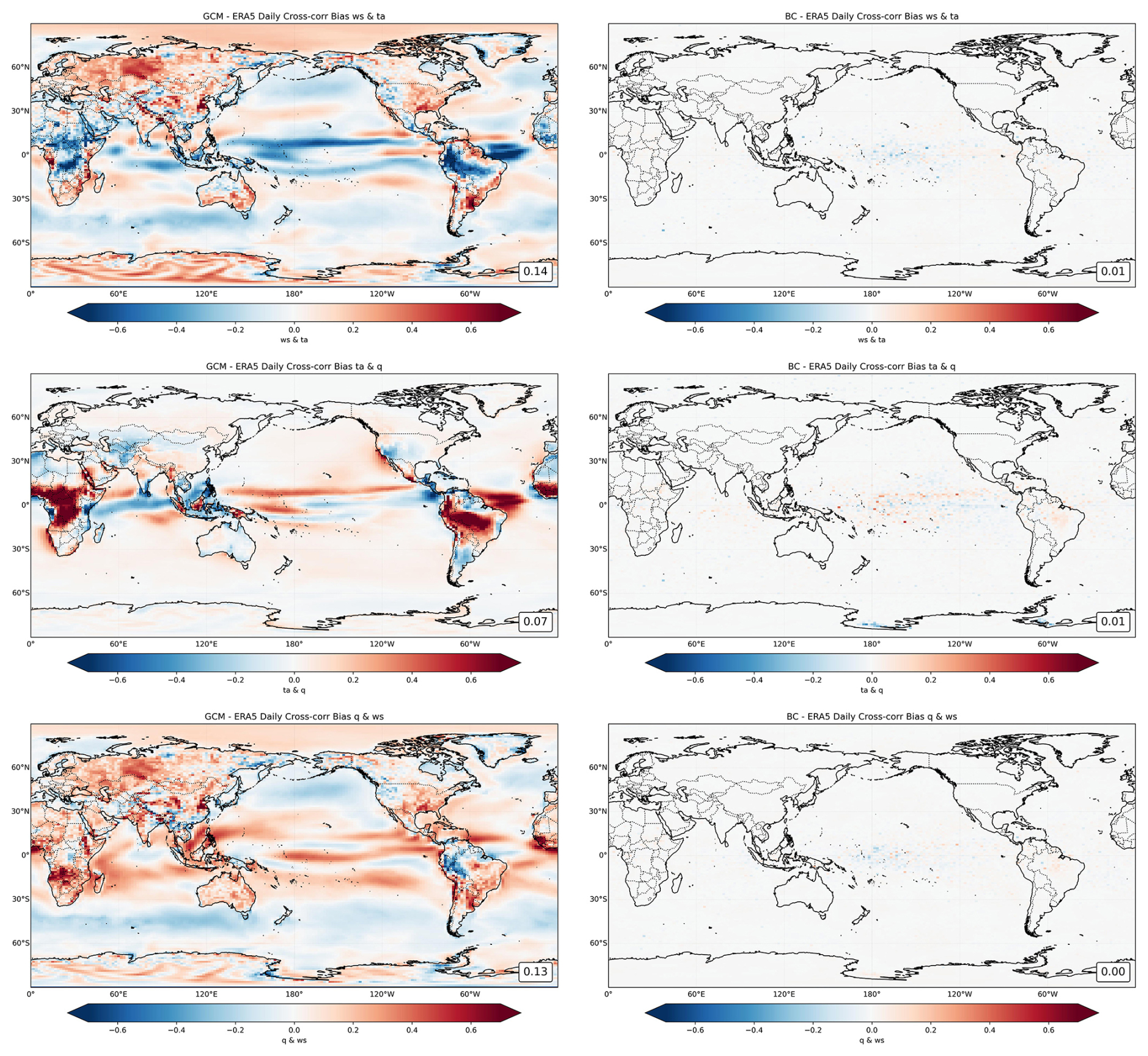
Figure 6 As in Fig. 3, but for lag0 cross-correlation.

Figure 6 presents bias maps for lag-0 cross-correlation, similar to Fig. 3. The uncorrected GCM exhibits notable cross-correlation biases, particularly in regions influenced by deep convection and strong large-scale circulation. For example, a positive bias in the cross-correlation between air temperature and specific humidity (ta and q) over tropical regions suggests an overestimated coupling between thermal and moisture fields. This could lead to exaggerated feedback in moist convection, ultimately distorting projections of heat stress and precipitation extremes. Similarly, the cross-correlations between wind speed and temperature (ws and ta), and wind speed and specific humidity (ws and q), display substantial regional biases, which may degrade the representation of energy and moisture fluxes essential for storm development and atmospheric stability.

In contrast, the bias-corrected outputs demonstrate near-zero deviations across most regions, indicating that SDMBCv2 effectively restores realistic inter-variable relationships.

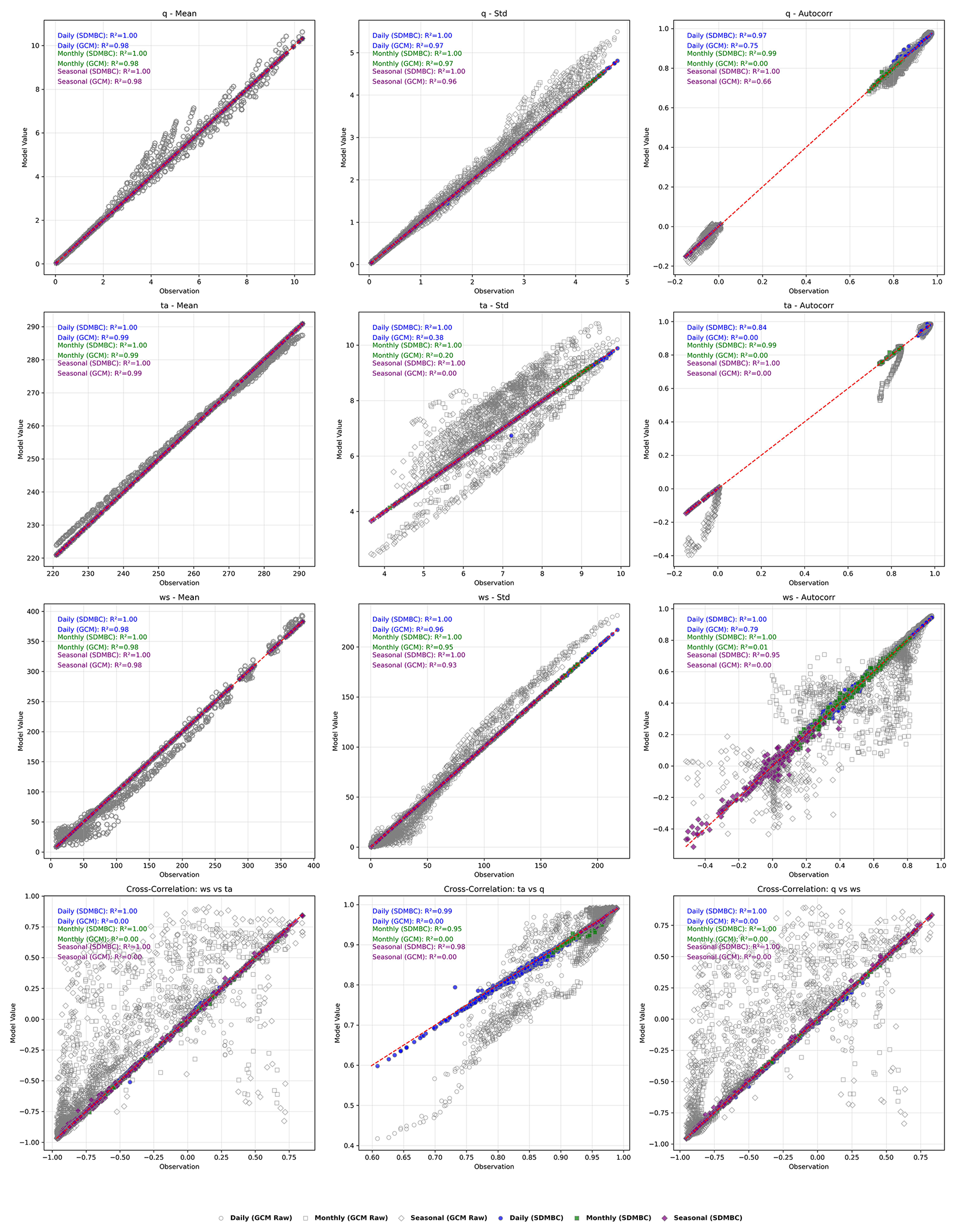
Figure 7 Scatter plot of atmospheric variables for climatological statistics across the vertical levels in the sampled domain in calibration periods from 1959 to 1989.

Figure 7 presents scatter plots comparing observed values with both uncorrected and bias-corrected GCM outputs for key atmospheric variables across 24 vertical levels within the study domain. To ensure reliability, levels where specific humidity approaches zero (i.e., here below 10⁻⁴), where statistical moments become unstable, were excluded from the analysis, following guidance from prior studies (Kim et al., 2023d).

The figure evaluates the impact of bias correction across multiple statistical measures: mean, standard deviation, lag1 auto-correlation, and lag0 cross-correlation, at different temporal scales, including daily, monthly, and seasonal. The results demonstrate a clear improvement following bias correction. Furthermore, the figure shows that the uncorrected GCM variables exhibit significant biases in inter-variable relationships, potentially leading to unrealistic atmospheric behavior. These biases can distort essential physical interactions such as moisture transport, energy exchange, and convective processes, ultimately affecting the reliability of regional climate projections. In contrast, the bias-corrected GCM variables align well with observed data, with most points clustering near the 45° line.

5.2 Bias-corrected GCM datasets: validation

This section evaluates the performance of the bias correction during the validation period (1990–2020), using the same spatial domain and variables applied during calibration. As in the calibration phase, the analysis includes sea surface temperature (SST) and key atmospheric variables, with selected grid cells examined to assess bias correction performance across vertical levels. The goal is to determine whether the improvements achieved during the calibration period are maintained over a distinct, independent time window and whether SDMBCv2 continues to reduce biases across multiple time scales and statistical dimensions.

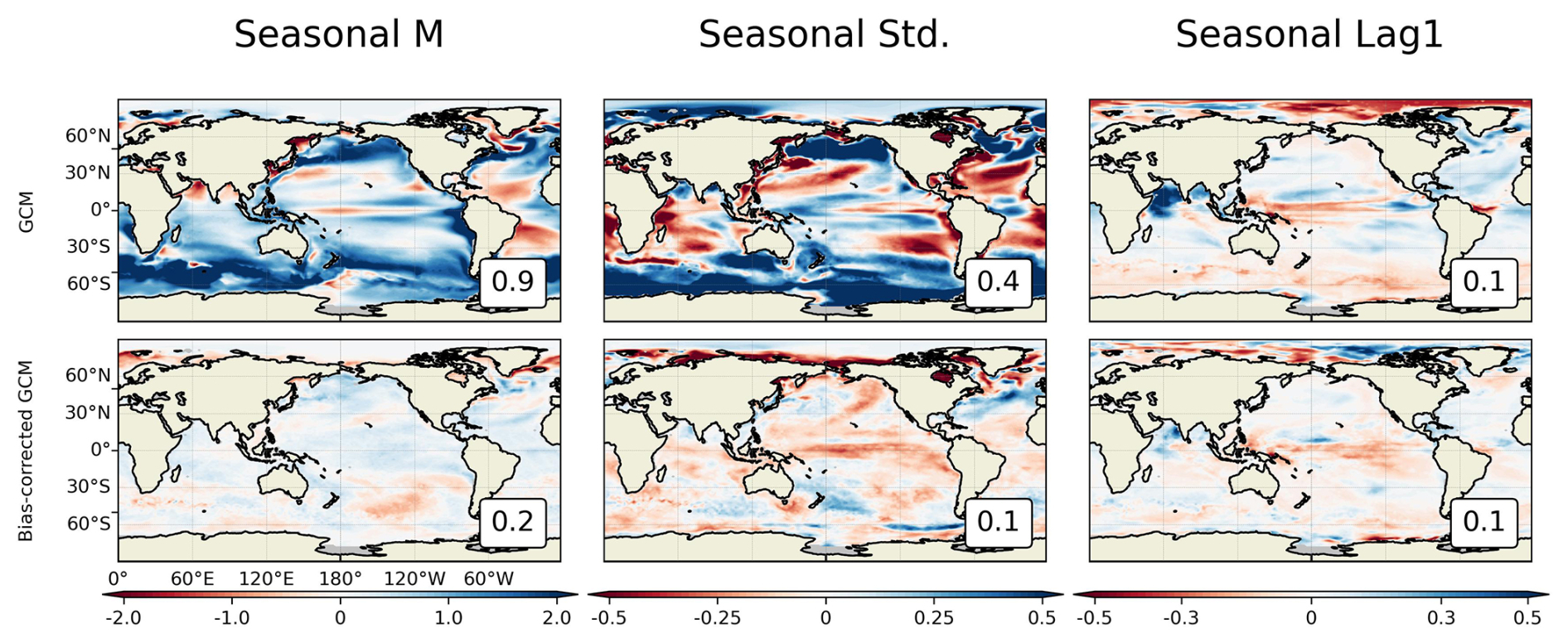
Figure 8 Seasonal bias map of sea surface temperature (SST) for both GCM and bias-corrected data in validation periods from 1990 to 2020. The number at the bottom right shows the mean absolute error.

Figure 8 illustrates seasonal SST bias maps comparing uncorrected and bias-corrected GCM outputs against ERA5 during the validation period. The results show substantial biases in the seasonal mean of the uncorrected GCM, particularly in the Southern Ocean and equatorial Pacific, where the mean absolute bias reaches approximately 0.9 °C. Following bias correction, these discrepancies are substantially reduced, with the global mean absolute bias decreasing to 0.2 °C. Notable improvements are observed in both high-latitude and tropical regions, where accurate SST representation is essential for resolving coupled ocean-atmosphere processes. The correction also reduces the bias in seasonal standard deviation from 0.4 °C in the raw GCM to 0.1 °C, with marked improvements in regions influenced by upwelling and in the North Atlantic. Furthermore, modest improvements are evident in seasonal lag-1 autocorrelation.

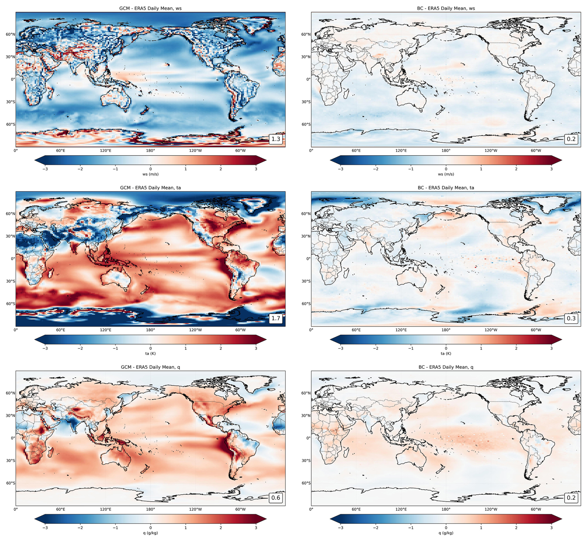
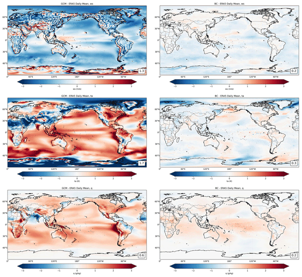
Figure 9 Bias maps of the climatological mean during the validation period (1990–2020), comparing uncorrected (GCM) and bias-corrected GCM outputs (BC) against ERA5 for three key atmospheric variables at the lowest model level. The left panels illustrate the raw GCM, while the right panels show the results after applying SDMBCv2. The number at the bottom right shows the mean absolute error.

Consistent with the calibration results, the uncorrected GCM from Fig. 9 exhibits substantial biases in all three variables: wind speed (ws) is strongly underestimated, air temperature (ta) shows widespread warm biases and specific humidity (q) is excessively high in tropical and mid-latitude regions. On the other hand, following bias correction, mean biases are considerably reduced across all regions. The post-correction fields show small residual errors, with global mean absolute biases reduced from 1.3 to 0.2 m s⁻¹ for wind speed, from 1.7 to 0.3 K for temperature, and from 0.6 to 0.2 g kg⁻¹ for specific humidity. These improvements confirm the robustness and generalizability of SDMBCv2 in reducing mean-state errors beyond the calibration period.

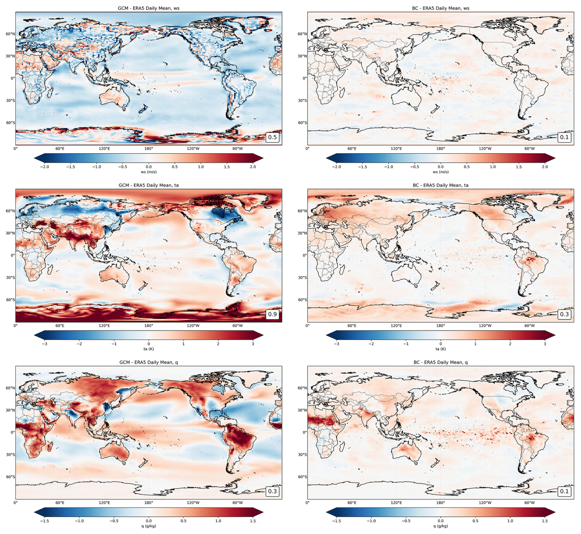
Figure 10 As in Fig. 9, but for standard deviation.

Figure 10 displays bias maps of the daily standard deviation during the validation period. The uncorrected GCM underestimates variability in the wind speed, with a global mean absolute bias of 0.5 m s⁻¹. Air temperature and specific humidity also exhibit widespread overestimation of variability, particularly in high-latitude and monsoon-influenced regions, with mean absolute biases of 0.9 K and 0.3 g kg⁻¹, respectively. On the other hand, after bias correction, variability biases are substantially reduced across the domain. The corrected fields show global mean absolute biases of 0.1 m s⁻¹ for wind speed, 0.3 K for temperature, and 0.1 g kg⁻¹ for specific humidity. Improvements are particularly evident in dynamically active regions, including the North Pacific, East Asia, and the Intertropical Convergence Zone, where realistic variability is essential for credible regional climate projections. However, some regions – such as parts of Africa – show a shift from negative to positive variability bias after correction; possible reasons for this are explored in the Discussion section. Overall, these results confirm the effectiveness of SDMBCv2 in adjusting not only mean-state conditions but also the amplitude of daily variability during an independent validation period.

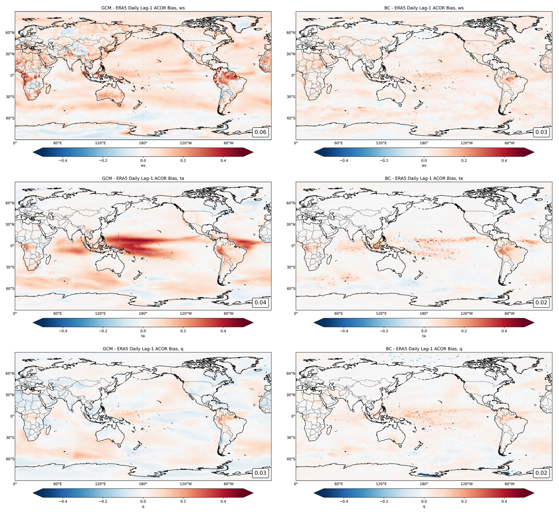
Figure 11 As in Fig. 9, but for lag1 auto-correlation.

Figure 11 presents bias maps of lag-1 autocorrelation for the validation period (1990–2020). Similar to the calibration period, the uncorrected GCM exhibits notable positive biases in temporal persistence, particularly for air temperature across the tropical oceans and for specific humidity in convective regions. These elevated autocorrelations suggest an overestimation of short-term memory effects, which can lead to unrealistic persistence of heat or moisture-related extremes, such as multi-day heatwaves or prolonged wet periods. Following bias correction, these biases are largely mitigated. The corrected outputs exhibit small deviations across most regions, demonstrating that SDMBCv2 can adjust the temporal structure of atmospheric variables and preserve the observed persistence characteristics during the independent validation period.

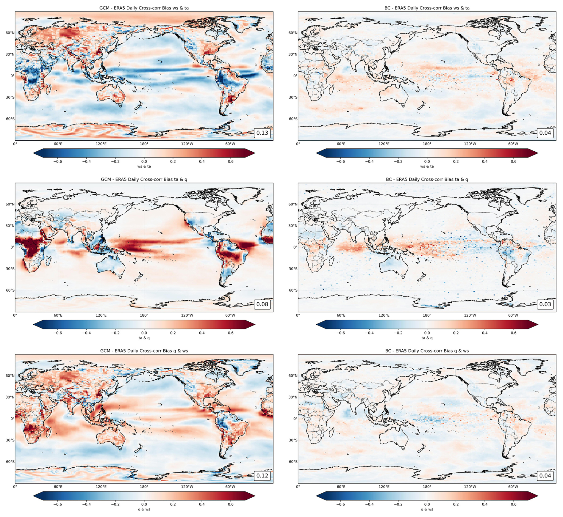
Figure 12 As in Fig. 9, but for cross-correlation.

Figure 12 shows bias maps of lag-0 cross-correlation for the validation period. In the uncorrected GCM, strong biases are evident in all variable pairings used in this study. These biases are most pronounced over tropical regions and convectively active zones, where the model tends to overestimate coupling strength. Such distortions can lead to unrealistic feedback in energy and moisture exchanges, ultimately affecting storm development, cloud formation, and precipitation processes.

After applying bias correction, cross-correlation biases are substantially reduced across most regions. The corrected fields exhibit only small bias, indicating that SDMBCv2 preserves key inter-variable dependencies and improves the physical consistency of atmospheric states. These results confirm the framework's ability to correct not only univariate statistical features but also the multivariate structure critical for realistic climate simulations.

Figure 13 As in Fig. 7, but for validation periods from 1990 to 2020.

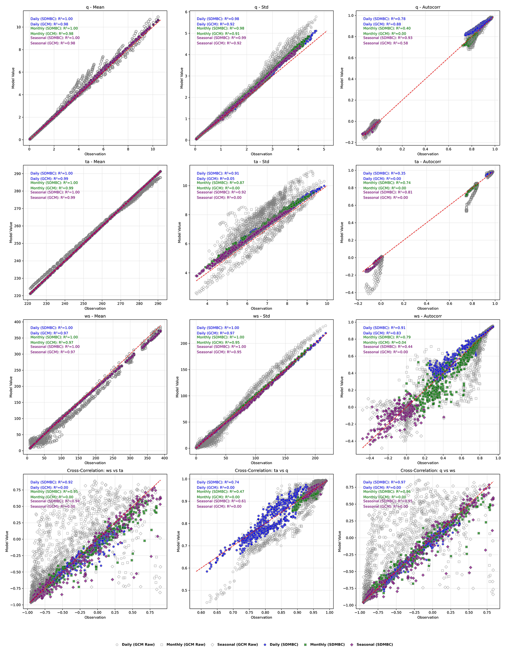
Figure 13 presents scatter plots similar to those in Fig. 7 but for the validation period (1990–2020). The results show that the bias-corrected GCM outputs consistently align more closely with reanalysis across all metrics, exhibiting improved accuracy and reduced dispersion compared to the raw GCM data. The uncorrected GCM outputs display considerable biases in both univariate and multivariate statistics. In contrast, the SDMBCv2-corrected outputs exhibit strong clustering around the 1:1 reference line across most metrics and time scales, indicating a well-aligned statistical structure with reanalysis.

Table 1 Percentage of grid cells passing the Kolmogorov–Smirnov (K–S) test at the 5 % significance level, comparing the distribution of GCM outputs (uncorrected and SDMBC-corrected) to ERA5 at four 6-hourly time steps (00:00, 06:00, 12:00, 18:00) during the calibration and validation periods. Variables tested include wind speed (ws), air temperature (ta), and specific humidity (q).

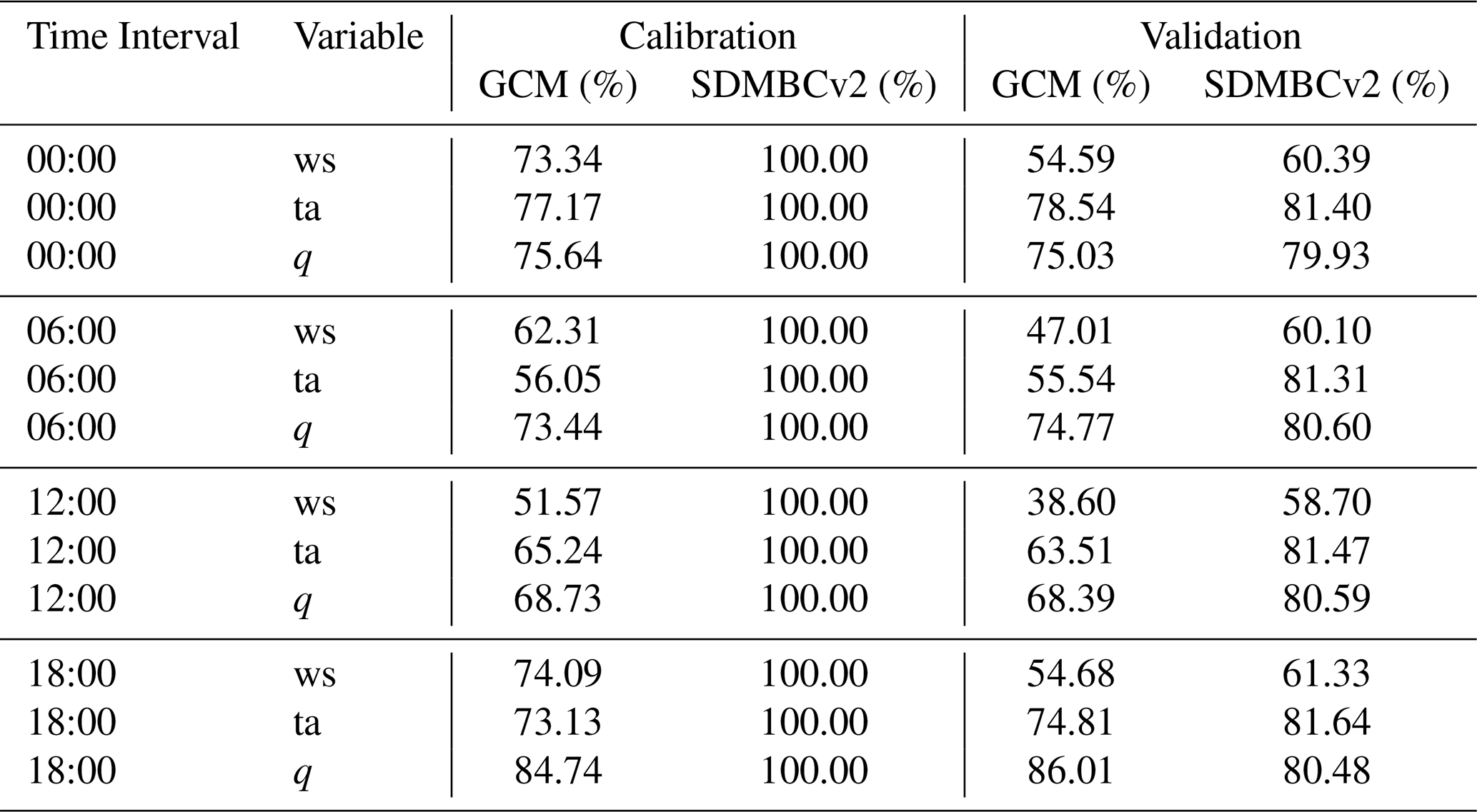
The results in Table 1 show a substantial improvement in distributional agreement with reanalysis following bias correction. During the calibration period, 100 % of sampled grid cells pass the K–S test for all variables and time steps after applying SDMBCv2, compared to notably lower rates in the raw GCM outputs. For example, raw GCM pass rates for wind speed range between 51 %–74 %.

During the validation period, SDMBCv2 improves distributional performance across most variables and time steps. For air temperature (ta), the percentage of grid cells passing the K–S test exceeds 81 % at all time steps after bias correction, compared to 56 %–78 % in the uncorrected GCM. Specific humidity (q) also shows consistent improvement at most times, with pass rates rising from 68 %–75 % in the raw GCM to 80 %–81 % following correction. However, at 18, the bias-corrected q pass rate (80.48 %) is slightly lower than that of the uncorrected GCM (86.01 %). This marginal reduction may reflect the challenge of correcting humidity distributions in regions with high variability and complex diurnal moisture cycles, where even small shifts in distribution shape can affect K–S test sensitivity.

For wind speed (ws), SDMBCv2 improves the pass rate by 5–20 percentage points at each time step, though the corrected values (58 %–61 %) remain modest compared to temperature and humidity.

6 Discussion and conclusion

This study evaluated the performance of the SDMBCv2 software, a Python package designed for sub-daily multivariate bias correction of GCM outputs used as boundary conditions for regional climate modeling. We focused on reducing systematic biases in atmospheric variables and SST across daily, monthly, and seasonal time scales. Our assessment involved comprehensive statistical evaluations against ERA5 reanalysis, using multiple metrics to test the consistency of corrected outputs during calibration (1959–1989) and an independent validation period (1990–2020).

The results consistently demonstrated that SDMBCv2 substantially reduces biases in GCM data, thereby improving the realism and reliability of simulated climate fields. Across all evaluated variables (wind speed, air temperature, and specific humidity) and statistical measures (mean, standard deviation, lag-1 autocorrelation, and lag-0 cross-correlation), the bias-corrected data exhibited marked improvement over the raw GCM simulations.

The analysis of climatological mean biases revealed that SDMBCv2 substantially corrects systematic errors in uncorrected GCM outputs. Large negative biases in wind speed, widespread warm biases in temperature, and excessive humidity across tropical and mid-latitude regions were minimized post-correction. These corrections have important implications, particularly for simulating climate extremes, where inaccuracies in atmospheric states can lead to unreliable projections of heatwaves, convective storms, and moisture-driven events.

SDMBCv2 also proved highly effective in adjusting variability metrics. Notably, the standard deviation biases were greatly reduced, reflecting an improved representation of temporal fluctuations essential for simulations of weather variability and associated phenomena, such as storm tracks, convective events, and boundary-layer processes. However, certain regions, notably parts of Africa, showed some residual or even increased variability biases post-correction. Several potential reasons were considered as follows. The observed standard deviation in these regions is very low (e.g., due to low moisture variability or stable conditions), and the correction may overcompensate when adjusting GCM variability. Multivariate corrections can induce indirect changes to a variable due to its coupling with others (e.g., correcting q in relation to ta). If temperature or wind speed is also adjusted in a way that enhances moisture variability, it could introduce an increased standard deviation in specific humidity, even if the raw bias was negative. It is also possible that the raw GCM's low variability was an artifact of its dynamics, whereas SDMBCv2 aligns its variability more closely with ERA5. While SDMBCv2 incorporates threshold-based safeguards to limit corrections under low-variability conditions (e.g., constraints on minimum variable magnitude and variance, and conditional skipping of variance adjustment when both model and observed variability are low), residual biases may still occur due to multivariate coupling effects, and these aspects require further exploration.

Another crucial strength of SDMBCv2 is its ability to maintain observed temporal and multivariate structures in GCM outputs. Lag-1 autocorrelation analysis indicated significant reductions in biases related to temporal persistence, highlighting the software's capability to prevent unrealistic short-term memory effects in the climate system. Additionally, SDMBCv2 maintained accurate cross-correlations among variables where uncorrected simulations showed substantial errors. For instance, the original GCM overestimated the coupling between air temperature and specific humidity, potentially inflating convective feedback; SDMBCv2 effectively corrected these interdependencies.

The validation period results further confirmed the robustness and generalizability of SDMBCv2. Bias corrections derived from the calibration period remained effective when applied to an independent validation period, maintaining similar levels of accuracy and consistency across multiple metrics. The Kolmogorov–Smirnov (K–S) tests provided strong statistical confirmation, showing marked improvements in distributional alignment between the corrected GCM outputs and ERA5. Specifically, the SDMBC-corrected datasets demonstrated generally high rates of passing the K–S test across all variables and times, contrasting sharply with the relatively poor performance of the raw GCM data.

Despite the notable improvements provided by SDMBCv2, several challenges remain. First, the correction quality inherently depends on the accuracy and reliability of the reanalysis benchmark (here, ERA5). Areas with limited in-situ observations or regions reliant primarily on satellite-based or modeled reanalysis products may present inherent uncertainties that propagate into the correction. Secondly, while SDMBCv2 generally preserves multivariate physical relationships, complex interactions in dynamically active or convectively dominant regions can pose challenges, potentially leading to locally increased biases. These aspects highlight the necessity for cautious interpretation of corrected outputs and further methodological refinements to address specific regional issues. Also, the perfect K–S test performance in the calibration period reflects the construction of the quantile mapping framework, while reduced pass rates in the independent validation period highlight the limited temporal transferability under changing conditions, including synoptic variability and potential non-stationarity of model biases. Although the bias-corrected fields mostly outperform the raw GCM, future work should investigate robustness across different calibration periods.

Future work should aim at reducing residual uncertainties and further enhancing the robustness of multivariate corrections. Integrating multiple observational datasets, potentially including satellite retrievals, could help provide more robust reference climatologies, particularly in poorly observed regions. Additionally, exploring advanced correction methodologies that better handle skewed or intermittent variables may further refine the representation of variability and extremes (Mehrotra and Sharma, 2019, 2021). It should also be worth noting that this study applies bias correction without explicitly preserving long-term trends, prioritizing the reduction of systematic biases in the baseline climatology. Future work may explore the integration of trend-preserving approaches, where appropriate, depending on the reliability of model-simulated climate change signals and the requirements of specific applications.

In conclusion, SDMBCv2 provides a powerful, flexible, and reliable tool for addressing systematic biases in GCM boundary conditions for regional climate modeling. SDMBCv2 facilitates improved climate modeling efforts, directly benefiting applications such as infrastructure planning, water resource management, and climate risk assessments. Continued development and refinement of this software promise further improvements in the fidelity and utility of regional climate simulations.