Comparison of two Euler equation sets in a Discontinuous Galerkin solver for atmospheric modelling (BRIDGE v0.9)

The implementation of a “classical” Discontinuous Galerkin (DG) solver for atmospheric flows is presented that is designed for efficient use in numerical weather prediction, climate simulations, and meteorological research both on the whole sphere and for limited area modeling. To this purpose the horizontally explicit, vertically implicit (HEVI) approach is used together with implicit-explicit (IMEX)-Runge-Kutta (RK) time integration schemes and a moderate spatial approximation order (order 4 or 5). Two Euler equation sets using mass, momentum and either density weighted potential temperature θ or total energy E as prognostic variables are compared by several idealised test cases. Details of the formulation of the Euler equations in covariant form using the Ricci tensor calculus, the linearisations needed for HEVI (especially for the total energy set), boundary conditions for an IMEX-RK scheme, and filtering for numerical stabilisation are given. Furthermore, the implementation of distributed memory parallelisation, the tensor product representation for prismatic grid cells, and optimisations for the HEVI formulation, are outlined. These developments lead to the so-called BRIDGE code, which will serve as a code base for a later DG extension of the well established ICON model. From the used idealised test cases, which are standard benchmarks for dynamical core development for the atmosphere, we conclude that the equation set using total energy E has better well-balancing properties than the set using θ. This result can be confirmed by a normal mode stability analysis. However, in some tests the set using E suffers more from non-linear instabilities that can only be partially solved by filtering.

1 Introduction

Among the numerous different methods to numerically solve partial differential equations, the Discontinuous Galerkin (DG) method has attracted a certain attention in many disciplines (fluid mechanics, elastomechanics, acoustics, electrodynamics, …) during the last decades since its first invention at the beginning of the 1970's (for a historical overview see Hesthaven and Warburton, 2008). The DG method allows to use quite arbitrary grid cells (triangles, prisms, hexagons, …) on arbitrary unstructured grids and runs efficiently on massively parallel computers due to very compact stencils. From a more numerical point of view DG methods can easily achieve higher order approximations, which highly increases accuracy for well resolved fields. However, in particular in fluid flows the fields are sometimes (or often) underresolved – here, another property of the DG method, namely its ability to treat every prognostic variable in a locally conserving manner (or better say: the flux divergence terms do not violate local conservation) helps in improving the physical consistency. Furthermore, DG methods in principle allow explicit time integration schemes, therefore one has a certain flexibility in the choice of an appropriate (explicit or implicit or combined) time discretisation.

After a few preliminary studies at the Deutscher Wetterdienst (DWD) about the usability of the DG method for atmospheric models (Brdar et al., 2012; Schuster et al., 2014; Baldauf, 2020, 2021) it was decided to start a new model development at DWD, called BRIDGE (Basic Research for ICON with DG Extension) (Baldauf and Prill, 2025). The new implementation is intended to be part of a DG version of the established ICON model (Zängl et al., 2015) later on. Therefore, its design aims to closely resemble and seamlessly integrate with ICON's Fortran codebase. The starting point for BRIDGE was the application of a DG scheme to solve the shallow water equations on a triangular grid on the sphere by Baldauf (2020) (in the following denoted as B20), and the solution of the Euler equations in terrain-following coordinates via the horizontally explicit, vertically implicit (HEVI) approach in a DG solver using implicit-explicit (IMEX)-Runge-Kutta (RK) time integration schemes by Baldauf (2021) (in the following denoted as B21). One result of these preliminary studies was that a spatial approximation order of about 4 seems to be adequate; grid irregularities don't play a role any more, but the cells are still small enough to benefit from local conservation. Additionally, the results showed that grid staggering is not necessary any more, a fact that simplifies coupling of parameterizations and coupling with geometrically separated subsystems like land, lake or ocean models.

One question in the design of a new dynamical core for atmospheric models is the choice of the prognostic variables, here in particular for the non-hydrostatic, compressible Euler equations (also see the different versions proposed in Giraldo et al., 2010 or Reddy et al., 2023). Since a DG scheme in general allows a better separation between the equation formulation and the pure numerical implementation this question seems less serious and is less a basic design issue than for other discretisation schemes (as e.g. finite difference schemes). Of course, one wants to keep the local conservation properties of the finite volume part of a DG scheme, therefore a flux form of the equations using density like variables (mass density, momentum instead of velocity, …) is preferred. However, it turns out, at least for the “classical” DG formulation used in the following, that the choice in particular of the thermodynamic variable is less arbitrary than expected. In B21, the density weighted potential temperature ρΘ was used, a choice that is made by several atmospheric simulation models as ICON (Zängl et al., 2015). Here, the use of ρΘ will be compared with the use of total energy density E (i.e. the sum of kinetic, potential and internal energy contributions), the latter is the preferred variable in computational fluid dynamics (CFD) simulation models.

The motivation to use total energy E of course stems from the fact that energy is one of the most fundamentally conserved variables in physics. Its conservation can be derived from time invariance of the physical laws (Noether's theorem), formulated as the first law in thermodynamics. Total energy further has the advantage to be quite unambiguously defined (there is no doubt about how to calculate kinetic, potential, internal, latent, … energy parts). On the other hand, if one restricts oneself to reversible processes and if the air does not change its constituents, the use of ρΘ implies local conservation of entropy (since in this case specific entropy s is related to potential temperature via s=c_plog Θ, where c_p is the specific heat capacity at constant pressure). Interestingly, local conservation of ρΘ still holds in the presence of diffusion (see Eqs. 6, 7, below), although entropy is not conserved for an irreversible process. However, in the more interesting atmospheric processes with change of moisture constituents, ρΘ is no longer an exactly conserved quantity. Beyond this, the definition of Θ is no longer unique in a moist atmosphere due to several possibilities which thermodynamic coefficients (R, c_p) should be used (the dry values or the moist values? Existence of other chemical or aerosol components, …). Although this is not a fundamental problem, it can become a practical one, if several parameterisations are coupled with a dynamical core (see also Reddy et al., 2023 for a few more properties of these two variable choices).

Therefore the purpose of this article is twofold. First, a DG implementation of a solver for atmospheric flows (BRIDGE) is presented that is designed for efficient use in numerical weather prediction, climate simulations, and meteorological research both on the whole sphere and for limited area modeling. Second, the influence of the choice of the prognostic variable ρΘ or total energy E in this framework will be investigated.

The article is organized as follows: Sect. 2 presents the two Euler equation sets in covariant (i.e. coordinate system independent) form and explains the concrete coordinate systems used in BRIDGE. Although there exist several attempts worldwide to develop DG based atmospheric models, our approach is different to most of them by using prismatic grid cells, to later on support the ICON user community. Our consistent usage of the covariant formalism allows to formulate the Euler equations on arbitrary manifolds while keeping basic DG properties, an aspect that might be of interest for other modelling communities, too. Section 3 explains the HEVI approach and in particular gives the needed linearisations for the energy form of the Euler equations. Our determination of the linearisation coefficients is slightly different from some other HEVI methods by omitting several terms, which can lead to a slightly higher efficiency. Several implementation details about parallelisation, usage of tensor products, and optimisations of the HEVI scheme are presented, too. The treatment of boundary conditions in IMEX time integration schemes is explained in Sect. 4. Filtering is used to prevent (mostly non-linear) instabilities and is explained in Sect. 5. Finally, Sect. 6 presents results from several atmospheric test cases.

2 Analytic formulations

2.1 Two Euler equation sets

In the following we write the Euler equations in covariant form, therefore valid in every arbitrary coordinate system. To this purpose we make extensive use of the Ricci tensor formalism (see B20, B21 and references therein), in particular we use the Einstein summation convention and sum over similar upper (contravariant) and lower (covariant) indices. Mass conservation is expressed by the continuity equation

$$\begin{array}{}\text{(1)}& {\displaystyle \frac{\partial \mathit{\rho }}{\partial t}}+{\mathrm{\nabla }}_k{M}^k=\mathrm{0}\end{array}$$

with mass density ρ and momentum density M^k. ∇_k denotes the covariant derivative; occasionally we use the denotation with a semicolon for it, e.g. ${\mathrm{\nabla }}_k{M}^i\equiv M_{;k}^i$.

The momentum balance equation is expressed as follows:

$$\begin{array}{}\text{(2)}& {\displaystyle \frac{\partial M^i}{\partial t}}+{\mathrm{\nabla }}_k{T}^{ik}=S_{\left(M\right)}^i\end{array}$$

with the momentum flux tensor for inviscid flow

$$\begin{array}{}\text{(3)}& T^{ik}=M^i{v}^k+p{g}^{ik},\end{array}$$

where $v^k=M^k/\mathit{\rho }$ denotes the velocity, p the pressure, and with the momentum source term consisting of buoyancy and Coriolis force

$$S_{\left(M\right)}^i=-\mathit{\rho }{g}^{ik}{\mathrm{\nabla }}_k\mathrm{\Phi }-\mathrm{2}{g}^{ij}{E}_{jkl}{\mathrm{\Omega }}^k{M}^l.$$

Here, Φ is the gravitational potential, Ω^k are the components of the angular velocity of the earth, g^ij the contravariant components of the metric tensor, E_jkl are the covariant components of the totally antisymmetric Levi-Civita tensor of rank 3 (analogous to the 2nd rank tensor given in B20).

In case of diffusion due to (turbulent) viscosity we add

$$\begin{array}{}\text{(4)}& T_{\left(D\right)}^{ik}=-\mathit{\rho }{K}_a\mathrm{2}{D}^{ik}-\mathit{\rho }{K}_b{g}^{ik}{\mathrm{\nabla }}_l{v}^l\end{array}$$

to the above momentum flux T^ik with the symmetric deformation tensor

$$D^{ik}={\displaystyle \frac{\mathrm{1}}{\mathrm{2}}}\left(g^{il}{\mathrm{\nabla }}_l{v}^k+g^{kl}{\mathrm{\nabla }}_l{v}^i\right).$$

As in B21, we use K_a=K_M and $K_b=-\frac{\mathrm{2}}{\mathrm{3}}{K}_{\mathrm{M}}$ with the kinematic shear viscosity K_M. In the test cases of Sect. 6 we either set $K_{\mathrm{M}}=\mathrm{const}.$ or use a mixing length approach

$$\begin{array}{}\text{(5)}& K_{\mathrm{M}}=l_{\mathrm{t}}^{\mathrm{2}}D,D=\sqrt{\mathrm{2}{D}_{ij}{D}^{ij}}\end{array}$$

(note the typo in the definition of the scalar shear D in B21). Here, l_t denotes a turbulent length scale (we specify one in Sect. 6.3).

In the following we will consider two variants of the energy balance:

2.1.1 Equation set “ρΘ”

Equation set “ρΘ” uses the density weighted potential temperature ϑ=ρΘ as the prognostic variable (this is the approach used in B21)

$$\begin{array}{}\text{(6)}& {\displaystyle \frac{\partial \mathit{\vartheta }}{\partial t}}+{\mathrm{\nabla }}_k{f}_{\left(\mathit{\vartheta }\right)}^k=S_{\left(\mathit{\vartheta }\right)},\end{array}$$

with the ϑ-flux for the pure Euler equations

$$f_{\left(\mathit{\vartheta }\right)}^k=v^k\mathit{\vartheta }.$$

In case of diffusion we add

$$\begin{array}{}\text{(7)}& f_{(\mathit{\vartheta },D)}^k=-\mathit{\rho }{K}_{\mathrm{H}}{g}^{kl}{\mathrm{\nabla }}_l\mathrm{\Theta }.\end{array}$$

This expression is motivated by the fact that there is no turbulent heat flux in a neutrally stratified atmosphere. In this article we use the simple (but generally not correct) assumption that the diffusion coefficient for heat K_H has the same value as K_M.

The pressure results from the equation of state for an ideal gas

$$p=p_{\mathrm{ref}}{\left({\displaystyle \frac{\mathit{\vartheta }{R}_d}{p_{\mathrm{ref}}}}\right)}^{c_p/c_v}$$

with a reference pressure usually chosen as p_ref=10⁵ Pa.

At the moment we only consider adiabatic processes (more specific: we have no energy sources/sinks due to latent heat release, chemical reactions, radioactive decay or radiation absorption/emission). Therefore, it holds S_(ϑ)=0.

2.1.2 Equation set “E”

As an alternative to Eq. (6) we use the balance equation for the total energy density E

$$\begin{array}{}\text{(8)}& {\displaystyle \frac{\partial E}{\partial t}}+{\mathrm{\nabla }}_k{f}_{\left(E\right)}^k=S_{\left(E\right)}.\end{array}$$

For adiabatic processes, we have no energy sources: S_(E)=0.

The total energy is the sum of kinetic, potential and internal energy $E=E_{\mathrm{kin}}+E_{\mathrm{pot}}+E_{\mathrm{int}}$ with components

$$\begin{array}{rl}{E}_{\mathrm{kin}}& ={\displaystyle \frac{\mathrm{1}}{\mathrm{2}}}{\displaystyle \frac{\mathrm{1}}{\mathit{\rho }}}{g}_{jk}{M}^j{M}^k,E_{\mathrm{pot}}=\mathit{\rho }\mathrm{\Phi }\left(\mathit{r}\right),\\ & E_{\mathrm{int}}=c_v\mathit{\rho }T.\end{array}$$

For given prognostic variables we can first determine the internal energy $E_{\mathrm{int}}=E-E_{\mathrm{kin}}-E_{\mathrm{pot}}$ and then calculate the temperature T. The pressure follows from the ideal gas equation

$$\begin{array}{}\text{(9)}& p=R\mathit{\rho }T\end{array}$$

with the individual gas constant R for air. Pressure also has a simple relationship with the internal energy

$$p={\displaystyle \frac{R}{c_v}}{E}_{\mathrm{int}}$$

and can be expressed by the prognostic variables via

$$\begin{array}{}\text{(10)}& p={\displaystyle \frac{R}{c_v}}\left(E-{\displaystyle \frac{\mathrm{1}}{\mathrm{2}}}{\displaystyle \frac{\mathrm{1}}{\mathit{\rho }}}{g}_{jk}{M}^j{M}^k-\mathit{\rho }\mathrm{\Phi }\right).\end{array}$$

The energy flux for the Euler equations is expressed as

$$\begin{array}{}\text{(11)}& f_{\left(E\right)}^k=v^k(E+p).\end{array}$$

In case of viscosity and heat conduction we add two diffusive flux contributions

$$\begin{array}{}\text{(12)}& {\displaystyle }{f}_{(E,Dk)}^k=v^j{g}_{jl}{T}_{\left(D\right)}^{kl},\text{(13)}& {\displaystyle }{f}_{(E,Dh)}^k=-K_{\mathrm{H}}\mathit{\rho }{c}_p{\displaystyle \frac{T}{\mathrm{\Theta }}}{g}^{kj}{\mathrm{\nabla }}_j\mathrm{\Theta }.\end{array}$$

The contribution $f_{(E,Dk)}^k$ can be derived from the full momentum flux tensor $T^{ik}+T_{\left(D\right)}^{ik}$ when considering the prognostic equation for the kinetic energy (see e.g. Landau and Lifshitz, 1987). Analogously, the contribution $f_{(E,Dh)}^k$ can be derived from the prognostic equation of the internal energy E_int using Eq. (7), note that this form exactly agrees with those given in Straka et al. (1993). In both these derivations, there occur source terms that contribute to changes of internal energy. However, the total energy is conserved. Written in the above given variables we can reformulate

$$\begin{array}{}\text{(14)}& f_{(E,Dh)}^k=-K_{\mathrm{H}}{g}^{kj}\left({\mathrm{\nabla }}_j{E}_{\mathrm{int}}-{\displaystyle \frac{c_p}{c_v}}{\displaystyle \frac{E_{\mathrm{int}}}{\mathit{\rho }}}{\mathrm{\nabla }}_j\mathit{\rho }\right).\end{array}$$

2.2 Use of a reference state

As in B21 we subtract a stationary, resting, and horizontally homogeneous reference state (denoted with subscript 0) that is in hydrostatic balance, and write the above prognostic equations for the deviations (denoted with a tilde), e.g. $\stackrel{\mathrm{̃}}{\mathit{\rho }}=\mathit{\rho }-{\mathit{\rho }}_{\mathrm{0}}$. In general, this improves the well-balancing problem in numerical discretisations of the pressure gradient and the buoyancy term in the momentum balance. Note that this reference state is not used for the linearisation later on in the HEVI scheme. In particular, for equation set “E” we subtract the reference state energy

$$\begin{array}{}\text{(15)}& E_{\mathrm{0}}={\mathit{\rho }}_{\mathrm{0}}\mathrm{\Phi }\left(\mathit{r}\right)+c_v{\mathit{\rho }}_{\mathrm{0}}{T}_{\mathrm{0}}={\mathit{\rho }}_{\mathrm{0}}\mathrm{\Phi }\left(\mathit{r}\right)+{\displaystyle \frac{c_v}{R}}{p}_{\mathrm{0}}.\end{array}$$

One possible choice is the isothermal atmosphere

$$\begin{array}{}\text{(16)}& T_{\mathrm{0}}\left(z\right)=T_{\mathrm{00}}=\mathrm{const}.,p_{\mathrm{0}}\left(z\right)=p_{\mathrm{ref}}(z=\mathrm{0})e^{-\frac{g}{R{T}_{\mathrm{00}}}z}.\end{array}$$

with the gravitational acceleration $g=\partial \mathrm{\Phi }/\partial z$ and ρ₀ following from the ideal gas Eq. (9). However, if not otherwise noted, we use the reference state

$$\begin{array}{}\text{(17)}& T_{\mathrm{0}}\left(z\right)=T_{\mathrm{ref},\mathrm{0}}+\mathrm{\Delta }{T}_{\mathrm{ref}}\left(e^{-\frac{z}{H_{\mathrm{ref}}}}-\mathrm{1}\right)\end{array}$$

from Zängl (2012), with $T_{\mathrm{ref},\mathrm{0}}=\mathrm{300}$ K, ΔT_ref=75 K, H_ref=10 000 m and the pressure at bottom $p_{\mathrm{ref}}(z=\mathrm{0})={\mathrm{10}}^{\mathrm{5}}$ Pa.

2.3 Coordinate systems

The above equations only use tensors (or products of two pseudo-tensors) and therefore are valid in every arbitrary coordinate system. As noted in B21, it is advantageous to rewrite these equations in the so-called strong-conservation form, because this reduces numerical violation of local conservation due to metric correction terms. This means that we now have two distinct coordinate systems K and K^′, where K^′ is “smoother” than K. For our purposes, K is a terrain-following coordinate system, whereas K^′ just follows the sphere (or even a flat plane). By this we can identically reformulate the scalar Eqs. (1), (6), or (8) as

$$\begin{array}{}\text{(18)}& {\displaystyle \frac{\partial \sqrt{g}\mathit{\varphi }}{\partial t}}+{\displaystyle \frac{\partial \sqrt{g}{f}_{\left(\mathit{\varphi }\right)}^k}{\partial x^k}}=\sqrt{g}{S}_{\left(\mathit{\varphi }\right)},\end{array}$$

where ϕ is ρ, ϑ or E, respectively, $f_{\left(\mathit{\varphi }\right)}^k$ is the related flux component, and S_(ϕ) is the related source term, and the momentum Eq. (2) (or any other prognostic equation for a vector field) as

$$\begin{array}{}\text{(19)}& {\displaystyle \frac{\partial \sqrt{g}{M}^{i^{\prime }}}{\partial t}}+{\displaystyle \frac{\partial }{\partial x^k}}\sqrt{g}{T}^{i^{\prime }k}=\sqrt{g}\left(S_{\left(M\right)}^{i^{\prime }}-{\mathrm{\Gamma }}_{l^{\prime }{k}^{\prime }}^{i^{\prime }}{T}^{l^{\prime }{k}^{\prime }}\right),\end{array}$$

with the scalar metric density g=detg_ij and the Christoffel symbol of second kind ${\mathrm{\Gamma }}_{l^{\prime }{k}^{\prime }}^{i^{\prime }}$.

Apart from these two types of prognostic equations we also have to deal with derivative variables for the treatment of diffusion via the BR1 scheme (Bassi and Rebay, 1997, also see Gassner et al., 2018). For these we use the form given in B21, Sect. 2.4, i.e. we consider the covariant derivative ϕ_;j of a scalar ϕ or the covariant derivative $M_{;j}^l$ of a vector field (with terrain-following components) M^l where the derivation is done by the terrain-following coordinate x^j.

Practically, we use the following sequence of coordinate systems and the related transformations¹:

1. For all input and output purposes, we use spherical coordinates

   $$x^{i^{\prime \prime }}=(\mathit{\lambda },\mathit{\varphi },z),z=r-r_{\mathrm{sphere}}$$

   on a sphere with given radius r_sphere. The metric properties of these coordinates and their transformations from/to Cartesian coordinates $x=x^{{\mathrm{1}}^{\prime \prime \prime }}$, $y=x^{{\mathrm{2}}^{\prime \prime \prime }}$, $z=x^{{\mathrm{3}}^{\prime \prime \prime }}$ are given in B20, Appendix A.

   Alternatively, for idealized tests we can use flat Cartesian coordinates. For convenience we also denote them as

   $$x^{i^{\prime \prime }}=(\mathit{\lambda },\mathit{\varphi },z),$$

   with the simple transformations from/to Cartesian coordinates

   $$x=R_x\mathit{\lambda },y=R_y\mathit{\varphi },z=z,R_x,R_y=\mathrm{const}.$$

2. On the sphere a triangulation is performed, i.e. all horizontal (2-dim.) grid cells are triangles. We map each of these spherical triangles onto unit triangles by a local gnomonial projection (Läuter et al., 2008) and call the related coordinate the local or unit coordinate² $x^{i^{\prime }}$ (note that there is no change in the vertical coordinate, i.e. $x^{{\mathrm{3}}^{\prime }}=x^{{\mathrm{3}}^{\prime \prime }}$). Consequently every triangle uses its own mapping and has its own coordinate system and related base vectors (and is therefore an example of a differentiable manifold). This means that tensor components change from one triangle to another. The gnomonial projection has the important property that points (in particular quadrature points) of both common edges of neighbouring spherical triangles are mapped to the same distances along the unit triangle edges.

   The metric properties of these coordinates and transformations between $x^{i^{\prime }}$ and $x^{i^{\prime \prime }}$ are given in B20, Appendix C (note that a slightly different notation of primes is used there).

3. To consider orography, we introduce terrain-following coordinates xⁱ, as in B21. They are defined by

   $$\begin{array}{}\text{(20)}& x^{\mathrm{1}}=x^{{\mathrm{1}}^{\prime }},x^{\mathrm{2}}=x^{{\mathrm{2}}^{\prime }},x^{\mathrm{3}}=f(x^{{\mathrm{1}}^{\prime }},x^{{\mathrm{2}}^{\prime }},x^{{\mathrm{3}}^{\prime }}).\end{array}$$

   The (user-defined) stretching function f may also depend on the orography $h_{\mathrm{oro}}(x^{{\mathrm{1}}^{\prime }},x^{{\mathrm{2}}^{\prime }})$ and the model top height H_top.

We use the usual transformation rules for (2nd rank) tensors to transform metric properties from one coordinate system to the next one,

$$g^{ij}={\displaystyle \frac{\partial x^i}{\partial x^{i^{\prime }}}}{\displaystyle \frac{\partial x^j}{\partial x^{j^{\prime }}}}{g}^{i^{\prime }{j}^{\prime }},g_{ij}={\displaystyle \frac{\partial x^{i^{\prime }}}{\partial x^i}}{\displaystyle \frac{\partial x^{j^{\prime }}}{\partial x^j}}{g}_{i^{\prime }{j}^{\prime }},$$

and for the Christoffel symbols (which are not tensors)

$${\mathrm{\Gamma }}_{jk}^i={\displaystyle \frac{\partial x^i}{\partial x^{i^{\prime }}}}{\displaystyle \frac{\partial x^{j^{\prime }}}{\partial x^j}}{\displaystyle \frac{\partial x^{k^{\prime }}}{\partial x^k}}{\mathrm{\Gamma }}_{j^{\prime }{k}^{\prime }}^{i^{\prime }}+{\displaystyle \frac{\partial x^i}{\partial x^{l^{\prime }}}}{\displaystyle \frac{{\partial }^{\mathrm{2}}{x}^{l^{\prime }}}{\partial x^j\partial x^k}}.$$

Note that throughout the entire DG framework (i.e. apart from input/output) we only use the terrain-following coordinate xⁱ as the independent coordinate (e.g. for derivatives) and the unit coordinate $x^{i^{\prime }}$ for the momentum components. Therefore, the above denotation of coordinates matches with the strong conservation form Eqs. (18) and (19) given above.

Finally, a remark should be made about the shallow atmosphere approximation in contrast to the deep version. In the deep case, nothing else must be done in the above described approach. However, all test cases below on the sphere use the shallow atmosphere approximation, and this approximation is still used by many global forecast models worldwide due to slight efficiency reasons. This means that in all metric properties in the above coordinate system 1. the radial coordinate $x^{{\mathrm{3}}^{\prime \prime }}+r_{\mathrm{sphere}}$ is replaced by the constant earth radius r_sphere. Consequently, all partial derivatives of the metric tensor by the radial coordinate vanish: ${\partial }_{{\mathrm{3}}^{\prime \prime }}{g}_{i^{\prime \prime }{j}^{\prime \prime }}=\mathrm{0}$. This implies that those components of the Christoffel symbol vanish for which at least one index is equal to 3: ${\mathrm{\Gamma }}_{j^{\prime \prime }{k}^{\prime \prime }}^{i^{\prime \prime }}=\mathrm{0}$ if $i^{\prime \prime }=\mathrm{3}$ or $j^{\prime \prime }=\mathrm{3}$ or $k^{\prime \prime }=\mathrm{3}$. These metric properties are then transformed to the subsequent coordinate systems. This procedure automatically generates the right metric properties for a shallow atmosphere (in particular the right divergence and advection terms, see e.g. Baldauf et al., 2014). The only thing left to do is to apply the so-called traditional approximation, i.e. to skip some Coriolis terms. This is done by setting the radial unit component of the earth rotation velocity vector only: ${\mathrm{\Omega }}^{{\mathrm{1}}^{\prime }}={\mathrm{\Omega }}^{{\mathrm{2}}^{\prime }}=\mathrm{0}$, ${\mathrm{\Omega }}^{{\mathrm{3}}^{\prime }}=\mathrm{\Omega }\sin \mathit{\varphi }$, with the geographical latitude ϕ and the earth angular velocity $\mathrm{\Omega }=\mathrm{7.29212}\times {\mathrm{10}}^{-\mathrm{5}}$ rad s⁻¹. The gravitational potential in the shallow case sounds Φ(r)=gz with either the radial direction z in spherical coordinates or the vertical direction z in Cartesian coordinates, and the gravitational acceleration g=9.80665 m s⁻².

3 The HEVI-DG discretisation

3.1 The HEVI approach and related linearisations

In most meteorological model applications, the grid cells, at least near the ground, have a much smaller vertical than horizontal extent. Therefore, the time step restrictions related to the vertically expanding fast sound waves in particular are severe. We use the well-known HEVI approach to overcome this and again follow B21. To this purpose, the fluxes are split into an explicitly treated part f_ex that contains all horizontal and the nonlinear vertical contributions, and an implicitly treated vertical, linear part f_im. The source terms are analogously split into slow, explicitly treated and fast and linear, implicitly treated parts. In its most general form these equations (independently from its tensorial rank, i.e. either the scalar Eq. 18 or the vector Eq. 19) can be written for any prognostic variable q^(σ) as

$$\begin{array}{}\text{(21)}& \begin{array}{rl}{\displaystyle \frac{\partial \sqrt{g}{q}^{\left(\mathit{\sigma }\right)}}{\partial t}}& +{\displaystyle \frac{\partial }{\partial x^k}}\sqrt{g}{f}_{\mathrm{ex}}^{\left(\mathit{\sigma }\right)k}+{\displaystyle \frac{\partial }{\partial x^{\mathrm{3}}}}\sqrt{g}{f}_{\mathrm{im}}^{\left(\mathit{\sigma }\right)\mathrm{3}}\\ & =\sqrt{g}{S}_{\mathrm{ex}}^{\left(\mathit{\sigma }\right)}+\sqrt{g}{S}_{\mathrm{im}}^{\left(\mathit{\sigma }\right)}.\end{array}\end{array}$$

The upper index σ enumerates the N_σ prognostic variables. It should be noted that the sequence of coordinate systems described in Sect. 2.3 always maps to unit cells (unit prisms in BRIDGE), therefore, we directly can identify the scalar metric density with the Jacobian $J\equiv \sqrt{g}$, as it is usually denoted in the finite element or DG/CG literature.

In the following sections we define the implicitly treated terms. To keep consistency, all remaining (mostly nonlinear) terms are treated explicitly (e.g. Giraldo et al., 2013). Therefore, we have

$$\begin{array}{}\text{(22)}& \begin{array}{rl}{f}_{\mathrm{ex}}^{\left(\mathit{\sigma }\right)\mathrm{1}}& =f^{\left(\mathit{\sigma }\right)\mathrm{1}},f_{\mathrm{ex}}^{\left(\mathit{\sigma }\right)\mathrm{2}}=f^{\left(\mathit{\sigma }\right)\mathrm{2}},\\ & f_{\mathrm{ex}}^{\left(\mathit{\sigma }\right)\mathrm{3}}=f^{\left(\mathit{\sigma }\right)\mathrm{3}}-f_{\mathrm{im}}^{\left(\mathit{\sigma }\right)\mathrm{3}},\\ & S_{\mathrm{ex}}^{\left(\mathit{\sigma }\right)}=S^{\left(\mathit{\sigma }\right)}-S_{\mathrm{im}}^{\left(\mathit{\sigma }\right)},\end{array}\end{array}$$

where f^(σ)j and S^(σ) are the complete (nonlinear) flux and source terms, and with the vertical flux and source term linearisations of the implicit terms

$$\begin{array}{}\text{(23)}& f_{\mathrm{im}}^{\left(\mathit{\sigma }\right)\mathrm{3}}=\sum _{{\mathit{\sigma }}^{\prime }=\mathrm{1}}^{\mathrm{2}{N}_{\mathit{\sigma }}}{\displaystyle \frac{\mathit{\delta }{f}^{\left(\mathit{\sigma }\right)\mathrm{3}}}{\mathit{\delta }{q}^{\left({\mathit{\sigma }}^{\prime }\right)}}}{q}^{\left({\mathit{\sigma }}^{\prime }\right)},S_{\mathrm{im}}^{\left(\mathit{\sigma }\right)}=\sum _{{\mathit{\sigma }}^{\prime }=\mathrm{1}}^{\mathrm{2}{N}_{\mathit{\sigma }}}{\displaystyle \frac{\mathit{\delta }{S}^{\left(\mathit{\sigma }\right)}}{\mathit{\delta }{q}^{\left({\mathit{\sigma }}^{\prime }\right)}}}{q}^{\left({\mathit{\sigma }}^{\prime }\right)}.\end{array}$$

The linearisation coefficients $\mathit{\delta }{f}^{\left(\mathit{\sigma }\right)\mathrm{3}}/\mathit{\delta }{q}^{\left({\mathit{\sigma }}^{\prime }\right)}$ and $\mathit{\delta }{S}^{\left(\mathit{\sigma }\right)}/\mathit{\delta }{q}^{\left({\mathit{\sigma }}^{\prime }\right)}$ can depend on the variables q^(σ), which are generally taken from a previous time step. In these sums, q^(σ) either can be the N_σ=5 prognostic variables ($q^{\left(\mathrm{1}\right)}=\stackrel{\mathrm{̃}}{\mathit{\rho }}$, q⁽²⁾=M¹, …) or, in anticipation of possible diffusion terms, the N_σ=5 vertical derivative variables ($q^{\left(\mathrm{6}\right)}={\stackrel{\mathrm{̃}}{\mathit{\rho }}}_{;\mathrm{3}}$, $q^{\left(\mathrm{7}\right)}=M_{;\mathrm{3}}^{\mathrm{1}}$, …). Giraldo et al. (2024) demonstrate that this linear HEVI approach (denoted as “LHEVI-PS” there) has superior efficiency properties (at similar numerical stability) compared to other HEVI schemes that treat all nonlinear terms in an implicit manner.

3.1.1 Linearisation for the equation set “ρΘ”

All the linearisations needed for equation set “ρΘ” are described in B21; see Sect. 2.5.1 therein for the pure Euler equations and Sect. 2.5.2 for the related diffusion terms. We notice that these linearisations are not done in a strict mathematical sense, but in a way that the linear state is relatively close to the actual state of the atmosphere and keeps near hydrostatic balance as much as possible.

3.1.2 Linearisation for the equation set “E”

The terms that are responsible for sound expansion are the pressure gradient in the momentum equation and the velocity divergence in the thermodynamic equation (here: the total energy equation). Additionally, an implicit treatment of the buoyancy term helps in stabilizing gravity wave expansion.

Therefore, we first have to look at the pressure deviation $\stackrel{\mathrm{̃}}{p}$ in the momentum equation. From Eq. (10) and the reference state energy, Eq. (15), we get

$$\begin{array}{}\text{(24)}& \stackrel{\mathrm{̃}}{p}=p-p_{\mathrm{0}}={\displaystyle \frac{R}{c_v}}\left(\stackrel{\mathrm{̃}}{E}-{\displaystyle \frac{\mathrm{1}}{\mathrm{2}}}{\displaystyle \frac{\mathrm{1}}{\mathit{\rho }}}{M}_j{M}^j-\stackrel{\mathrm{̃}}{\mathit{\rho }}\mathrm{\Phi }\right).\end{array}$$

Though this is an exact expression, $\stackrel{\mathrm{̃}}{E}$ arises only in a linear manner, the same holds for $\stackrel{\mathrm{̃}}{\mathit{\rho }}$ in the third term. This is the main reason why there is no problem with using the potential energy: any shift in the geopotential exactly cancels in the first and third term. At a first glance, a linearisation just in these two variables $\stackrel{\mathrm{̃}}{\mathit{\rho }}$ and $\stackrel{\mathrm{̃}}{E}$ (i.e. without the kinetic energy term) should be sufficient for an implicit and therefore stable treatment of the vertically expanding sound waves. However, since the full pressure gradient is important, it turns out that the kinetic energy term must be linearised, too, in the momentum derivatives of the momentum flux to get a stable behaviour.

So, for the pure Euler equations (set “E”) we express the fluxes (3), (11) by the prognostic variables $\stackrel{\mathrm{̃}}{\mathit{\rho }}$, $M^{j^{\prime }}$ and $\stackrel{\mathrm{̃}}{E}$ and can derive the following linearisations just by differentiation: for the mass flux

$$\textcolor{red}{}$$

for the momentum fluxes

$$\begin{array}{}\text{(25)}& \textcolor{red}{}\end{array}$$

and for the energy flux

$${\displaystyle }\textcolor{red}{}$$

We want to emphasize that these linearisation coefficients depend on the actual or at least recent state $q^{\left(\mathit{\sigma }\right)}=q_{\mathrm{0}}^{\left(\mathit{\sigma }\right)}+{\stackrel{\mathrm{̃}}{q}}^{\left(\mathit{\sigma }\right)}$ of the atmosphere and not only on the reference state $q_{\mathrm{0}}^{\left(\mathit{\sigma }\right)}$. As discussed above not every term is necessary for a stable treatment of sound and gravity waves and in fact we only use the underlined terms. In particular, we neglect linearisations by E or ρ in the energy flux and skip terms that are quadratic in the momentum variables in general. The omittance of these terms is mainly done by efficiency reasons; they also seem to have in general only a minor influence. We have found experimentally that one can even set $\frac{\mathit{\delta }{T}^{i^{\prime }\mathrm{3}}}{\mathit{\delta }{M}^{{\mathrm{3}}^{\prime }}}=\mathrm{0}$ without detrimental effects, because this omission can slightly reduce a nonlinear instability when the vertical momentum $M^{{\mathrm{3}}^{\prime }}$ starts to oscillate. However we have seen (e.g. by the simple 1D test case in Sect. 6.1 with a horizontal base flow), that the following two terms need a special treatment, which otherwise would lead to strong overshooting of vertical velocity near the top and bottom boundaries. First, the underlined term denoted as “factor $\mathrm{1}/\mathrm{2}$” stems from the kinetic energy (by the pressure term in the momentum flux) and, as a quadratic term in the velocity, it is taken only with a factor $\mathrm{1}/\mathrm{2}$. Second, the term ∼E_kin in Eq. (25) should be omitted, too. These particular choices are motivated by the fact that the implicit momentum flux then exactly results in the pressure perturbation (use Eq. 24)

$$\begin{array}{rl}{f}_{\mathrm{im}}^{\left(M^{i^{\prime }}\right)\mathrm{3}}& ={\displaystyle \frac{\mathit{\delta }{T}^{i^{\prime }\mathrm{3}}}{\mathit{\delta }\mathit{\rho }}}\stackrel{\mathrm{̃}}{\mathit{\rho }}+{\displaystyle \frac{\mathit{\delta }{T}^{i^{\prime }\mathrm{3}}}{\mathit{\delta }{M}^{k^{\prime }}}}{M}^{k^{\prime }}+{\displaystyle \frac{\mathit{\delta }{T}^{i^{\prime }\mathrm{3}}}{\mathit{\delta }E}}\stackrel{\mathrm{̃}}{E}\\ & ={\displaystyle \frac{R}{c_v}}\left(-\stackrel{\mathrm{̃}}{\mathit{\rho }}\mathrm{\Phi }-{\displaystyle \frac{\mathrm{1}}{\mathrm{2}\mathit{\rho }}}{M}_{k^{\prime }}{M}^{k^{\prime }}+\stackrel{\mathrm{̃}}{E}\right)g^{i^{\prime }\mathrm{3}}=\stackrel{\mathrm{̃}}{p}{g}^{i^{\prime }\mathrm{3}},\end{array}$$

which helps to improve hydrostatic well-balancing in the implicit part. We want to remark that this is a slightly different linearisation strategy as e.g. used in Souza et al. (2023) or Giraldo et al. (2024).

Apart from these flux term linearisations we only have one source term to linearise, namely the buoyancy term in the momentum equation with

$${\displaystyle \frac{\mathit{\delta }{S}_{\left(M\right)}^{{\mathrm{3}}^{\prime }}}{\mathit{\delta }\mathit{\rho }}}=-g^{{\mathrm{3}}^{\prime }{\mathrm{3}}^{\prime }}{\mathrm{\nabla }}_{{\mathrm{3}}^{\prime }}\mathrm{\Phi }.$$

All other implicit source term coefficients in Eq. (23) are set to zero.

In case of diffusion, we get the linearisations as follows. There is no diffusion term in the continuity equations. The diffusive term in the momentum equation does not depend on the thermodynamic variable, therefore we use the same as for equation set “ρΘ”. The diffusive energy flux $f_{(E,Dh)}^{\mathrm{3}}$, Eq. (14), can be linearised by the prognostic and vertical derivative variables to give

$$\begin{array}{rl}{f}_{(E,D,\mathrm{lin})}^{\mathrm{3}}& ={\displaystyle \frac{\mathit{\delta }{f}_{E,D}^{\mathrm{3}}}{\mathit{\delta }\mathit{\rho }}}\stackrel{\mathrm{̃}}{\mathit{\rho }}+{\displaystyle \frac{\mathit{\delta }{f}_{E,D}^{\mathrm{3}}}{\mathit{\delta }{M}^{j^{\prime }}}}{M}^{j^{\prime }}+{\displaystyle \frac{\mathit{\delta }{f}_{E,D}^{\mathrm{3}}}{\mathit{\delta }E}}\stackrel{\mathrm{̃}}{E}\\ & +{\displaystyle \frac{\mathit{\delta }{f}_{E,D}^{\mathrm{3}}}{\mathit{\delta }{\mathit{\rho }}_{;\mathrm{3}}}}{\stackrel{\mathrm{̃}}{\mathit{\rho }}}_{;\mathrm{3}}+{\displaystyle \frac{\mathit{\delta }{f}_{E,D}^{\mathrm{3}}}{\mathit{\delta }{M}_{;\mathrm{3}}^k}}{M}_{;\mathrm{3}}^k+{\displaystyle \frac{\mathit{\delta }{f}_{E,D}^{\mathrm{3}}}{\mathit{\delta }{E}_{;\mathrm{3}}}}{\stackrel{\mathrm{̃}}{E}}_{;\mathrm{3}},\end{array}$$

with the linearisation coefficients

$$\begin{array}{c}{\displaystyle }\begin{array}{rl}{\displaystyle \frac{\mathit{\delta }{f}_{E,D}^{\mathrm{3}}}{\mathit{\delta }\mathit{\rho }}}& =-K_{\mathrm{H}}{g}^{\mathrm{3}j}\left[-\left(\mathrm{1}+{\displaystyle \frac{c_p}{c_v}}\right){\displaystyle \frac{\mathrm{1}}{{\mathit{\rho }}^{\mathrm{3}}}}{M}^{k^{\prime }}{M}_{k^{\prime }}{\mathit{\rho }}_{;j}\right.\\ & \left.+{\displaystyle \frac{c_p}{c_v}}{\displaystyle \frac{E}{{\mathit{\rho }}^{\mathrm{2}}}}{\mathit{\rho }}_{;j}-g{\displaystyle \frac{\partial x^{{\mathrm{3}}^{\prime }}}{\partial x^j}}+{\displaystyle \frac{\mathrm{1}}{{\mathit{\rho }}^{\mathrm{2}}}}{M}_{;j}^k{M}_k\right],\end{array}\\ {\displaystyle \frac{\mathit{\delta }{f}_{E,D}^{\mathrm{3}}}{\mathit{\delta }{M}^{j^{\prime }}}}=-K_{\mathrm{H}}{g}^{\mathrm{3}j}\left[\left(\mathrm{1}+{\displaystyle \frac{c_p}{c_v}}\right){\displaystyle \frac{\mathrm{1}}{{\mathit{\rho }}^{\mathrm{2}}}}{\mathit{\rho }}_{;j}{M}_{j^{\prime }}-{\displaystyle \frac{\mathrm{1}}{\mathit{\rho }}}{M}_{;j}^k{\displaystyle \frac{\partial x^{k^{\prime }}}{\partial x^k}}{g}_{k^{\prime }{j}^{\prime }}\right],\\ {\displaystyle }\begin{array}{rl}{\displaystyle \frac{\mathit{\delta }{f}_{E,D}^{\mathrm{3}}}{\mathit{\delta }E}}& =K_{\mathrm{H}}{g}^{\mathrm{3}j}{\displaystyle \frac{c_p}{c_v}}{\displaystyle \frac{\mathrm{1}}{\mathit{\rho }}}{\mathit{\rho }}_{;j},\\ & {\displaystyle \frac{\mathit{\delta }{f}_{E,D}^{\mathrm{3}}}{\mathit{\delta }{\mathit{\rho }}_{;\mathrm{3}}}}=-K_{\mathrm{H}}{g}^{\mathrm{33}}\left[{\displaystyle \frac{\mathrm{1}}{\mathrm{2}}}{\displaystyle \frac{\mathrm{1}}{{\mathit{\rho }}^{\mathrm{2}}}}{M}^{k^{\prime }}{M}_{k^{\prime }}-\mathrm{\Phi }-{\displaystyle \frac{c_p}{c_v}}{\displaystyle \frac{E_{\mathrm{int}}}{\mathit{\rho }}}\right],\end{array}\\ {\displaystyle \frac{\mathit{\delta }{f}_{E,D}^{\mathrm{3}}}{\mathit{\delta }{M}_{;\mathrm{3}}^k}}=K_{\mathrm{H}}{g}^{\mathrm{33}}{\displaystyle \frac{\mathrm{1}}{\mathit{\rho }}}{M}_k,{\displaystyle \frac{\mathit{\delta }{f}_{E,D}^{\mathrm{3}}}{\mathit{\delta }{E}_{;\mathrm{3}}}}=-K_{\mathrm{H}}{g}^{\mathrm{33}}.\end{array}$$

Note that we skip all linearisations related to the inherently quadratic diffusive momentum flux contribution f_E,Dk. Up to now, we have not seen stability problems by not treating f_E,Dk implicitly.

All these linearisation coefficients are calculated (“updated”) only after every 50 timesteps, to reduce the effort of performing the expensive LU decomposition. This is supported by the fact that we only use SDIRK IMEX-RK schemes, where the diagonal RK coefficients of the implicit part are all the same. Therefore, we can use the same matrices for the implicit back-substitution, matrix-vector multiplications for all RK stages during 50 time steps. However, for the baroclinic instability test, Sect. 6.6, and the Held and Suarez (1994) test, Sect. 6.7, the time steps are so large, that a higher frequency of every 10 timesteps is partly necessary for numerical stability.

3.2 The DG scheme

In this section, we describe the basic steps towards a “classical” DG-scheme (Cockburn and Shu, 1989; Cockburn et al., 1989, 1990; Hesthaven and Warburton, 2008) for the Euler equations in strong conservation form. Here, we only present the basic formulation, details about the HEVI formulation can be found in B21. The 3D domain is divided into N_hc×N_vc non-overlapping prismatic cells ${\mathrm{\Omega }}_{jk}=E_j\times I_k$, where the index $j=\mathrm{1},\mathrm{\dots },N_{\mathrm{hc}}$ enumerates the cells in the horizontal directions. and $k=\mathrm{1},\mathrm{\dots },N_{\mathrm{vc}}$ enumerates in the vertical direction. This means that the BRIDGE code makes the common assumption of an unstructured columnar mesh (prismatic cells): each grid cell of the horizontal mesh corresponds to a vertical column extending radially upward. As mentioned in Sect. 3.1, we assume that the coordinate transformation already maps onto unit cells in the system K. Therefore, the vertical interval is the unit interval $I_k=[-\mathrm{1},+\mathrm{1}]$ and in the horizontal we have unit triangles $E_j=\mathit{\left\{}\right(x^{\mathrm{1}},x^{\mathrm{2}}\left)\right|-\mathrm{1}\le x^{\mathrm{1}}\le \mathrm{1},-\mathrm{1}\le x^{\mathrm{2}}\le x^{\mathrm{1}}\mathit{\}}$.

The weak form is achieved by multiplication of the general Eq. (21) with a test function v over the cell Ω_jk and integration by parts

$$\begin{array}{}\text{(26)}& \begin{array}{rl}{\displaystyle \frac{\mathrm{d}}{\mathrm{d}t}}& \underset{{\mathrm{\Omega }}_{jk}}{\int }\sqrt{g}{q}^{\left(\mathit{\sigma }\right)}v\mathrm{d}V=-\underset{\partial {\mathrm{\Omega }}_{jk}}{\int }\sqrt{g}v{f}_{\mathrm{ex}}^{\left(\mathit{\sigma }\right)k,\mathrm{num}}{n}_k\mathrm{d}a\\ & -\underset{\partial {\mathrm{\Omega }}_{jk}}{\int }\sqrt{g}v{f}_{\mathrm{im}}^{\left(\mathit{\sigma }\right)\mathrm{3},num}{n}_{\mathrm{3}}\mathrm{d}a\\ & +\underset{{\mathrm{\Omega }}_{jk}}{\int }\sqrt{g}{f}_{\mathrm{ex}}^{\left(\mathit{\sigma }\right)k}{\displaystyle \frac{\partial v}{\partial x^k}}\mathrm{d}V+\underset{{\mathrm{\Omega }}_{jk}}{\int }\sqrt{g}{f}_{\mathrm{im}}^{\left(\mathit{\sigma }\right)\mathrm{3}}{\displaystyle \frac{\partial v}{\partial x^{\mathrm{3}}}}\mathrm{d}V\\ & +\underset{{\mathrm{\Omega }}_{jk}}{\int }\sqrt{g}{S}_{\mathrm{ex}}^{\left(\mathit{\sigma }\right)}v\mathrm{d}V+\underset{{\mathrm{\Omega }}_{jk}}{\int }\sqrt{g}{S}_{\mathrm{im}}^{\left(\mathit{\sigma }\right)}v\mathrm{d}V,\end{array}\end{array}$$

where n denotes the surface unit normal vector that is directed outwards of cell Ω_jk, dV is the volume element, and da the surface element.

As mentioned earlier, the classical BR1 scheme is used to handle the second-order diffusive terms. Therefore, the original set of equations is reformulated into a system of coupled first-order equations and 3N_σ auxiliary variables representing gradients are introduced.

For the numerical flux of the variable q^(σ) in direction n (which directs from “_L” to “_R”) we use the local Lax-Friedrichs (LF) flux (also known as Rusanov flux)

$$\begin{array}{}\text{(27)}& \begin{array}{rl}& f^{\left(\mathit{\sigma }\right)k,\mathrm{num}}{n}_k\equiv f^{\left(\mathit{\sigma }\right)\mathrm{num}}(q_{\mathrm{R}},q_{\mathrm{L}},\mathit{n})\\ & ={\displaystyle \frac{\mathrm{1}}{\mathrm{2}}}\left(f_{\mathrm{R}}^{\left(\mathit{\sigma }\right)j}+f_{\mathrm{L}}^{\left(\mathit{\sigma }\right)j}\right)n_j-{\displaystyle \frac{\mathit{\lambda }\left(\mathit{n}\right)}{\mathrm{2}}}(q_{\mathrm{R}}^{\left(\mathit{\sigma }\right)}-q_{\mathrm{L}}^{\left(\mathit{\sigma }\right)}).\end{array}\end{array}$$

Note that the LF-flux has the usual antisymmetry property $f^{\left(\mathit{\sigma }\right)\mathrm{num}}(q_{\mathrm{L}},q_{\mathrm{R}},-\mathit{n})=-f^{\left(\mathit{\sigma }\right)\mathrm{num}}(q_{\mathrm{R}},q_{\mathrm{L}},\mathit{n})$, which guarantees local conservation on a cell-wise level. This flux is used both for the hyperbolic explicit part and for the implicit part with suitable “diffusion velocities” λ_ex and λ_im, respectively (Blaise et al., 2016). The diffusion velocity for the Euler equations at the edge with unit normal vector n is known to be the sum of the speed of sound and the absolute value of the advective velocity

$$\begin{array}{rl}{\mathit{\lambda }}_{\mathrm{tot}}\left(\mathit{n}\right)& =G{c}_{\mathrm{snd}}+\left|n_i{v}^i\right|,c_{\mathrm{snd}}=\sqrt{{\displaystyle \frac{c_p}{c_v}}{\displaystyle \frac{p}{\mathit{\rho }}}},\\ & G=\sqrt{n_i{n}_j{g}^{ij}}.\end{array}$$

The derivation in particular of the metric factors is done analogous to those in B20 (Appendix D) for the shallow-water equations. According to Blaise et al. (2016), λ_tot is split into explicit and implicit contributions

$${\mathit{\lambda }}_{\mathrm{ex}}\left(\mathit{n}\right)=\left|G{c}_{\mathrm{snd}}{n}_{\mathrm{hor}}\right|+\left|n_i{v}^i\right|,{\mathit{\lambda }}_{\mathrm{im}}\left(\mathit{n}\right)={\mathit{\lambda }}_{\mathrm{tot}}\left(\mathit{n}\right)-{\mathit{\lambda }}_{\mathrm{ex}}\left(\mathit{n}\right).$$

n_hor denotes the horizontal part of n.

As mentioned in Sect. 2.3, every triangle uses its own coordinate base vectors, therefore we have to transform the horizontal, physical flux components f¹ and f² and the diffusion velocity λ at the horizontal edges of two neighbouring prisms, so that each cell can calculate its own numerical flux, as is described in B20, Sect. 3. Note that such a transformation does not interfere at all with the purely vertical implicit treatment of the HEVI approach. Furthermore, this symmetric flux transformation does not violate the local conservation property (see the proof in B20, Appendix E). In contrast, in the application of the BR1 scheme for diffusion, we exchange the derivative variables instead of the related “pseudo fluxes”. The reason for this different treatment is that the flux calculations of the Euler equations (in particular the additional diffusion terms) is relatively expensive, therefore it is efficient to calculate them only once and then transform to the neighbouring cell face. A flux has one tensorial rank more than its related prognostic variable, therefore the transformation is a bit costlier than it would be for the variable itself. Conversely in case of the derivative variables, the “pseudo flux” calculation is computationally cheap and it is therefore better to perform the flux calculation twice without the transformation.

The linear system of equations (LSE) resulting from the implicit part of the HEVI equations is given in B21, Sect. 3. This LSE defines one stage for an IMEX-RK time integration scheme. In contrast to the SSP3(4,3,3) scheme that was preferably used in B21, here we will mostly use the SSP3(3,3,2) scheme (Pareschi and Russo, 2005), whose implicit part is L-stable and whose explicit part is a strong stability preserving (SSP) 3rd order RK scheme, too (although we don't really benefit from the SSP property at the moment, since an Euler forward step is not stable by itself). Although its overall accuracy is only second order, we use it in BRIDGE due to higher efficiency because, firstly, this 3-stage scheme saves one implicit solve per timestep compared to the 4-stage SSP3(4,3,3) scheme, and secondly it allows a larger Courant number of about 0.12 for the linear advection equation with two velocities compared to about 0.08 for SSP3(4,3,3) (see B21, Table 1).

3.3 Remarks about the numerical implementation

3.3.1 Remarks about parallelization

One advantage of DG methods is their high computational intensity because of their high-order polynomial approximations and the large number of degrees of freedom in each element. Additionally, the locality of DG – requiring only face-neighbour data – allows for excellent weak and strong scaling on distributed-memory systems via domain decomposition. MPI (Message Passing Interface) enables DG parallelization with ghost exchanges for faces in two different forms:

In the first variant, one process calculates the numerical flux from the double-valued surface states and communicates the fluxes back to the neighbouring process (Krais et al., 2021). This parallelization strategy does not offer performance advantages for BRIDGE, as the fluxes for one side are not uniform due to the mapping: Since we use local coordinates on the sphere, we get different numerical fluxes for the right and the left cell.

Therefore, the BRIDGE code implementation employs the second variant, where only the trace of the solution has to be sent to the neighbouring partition while the partition boundary fluxes are evaluated twice (Kronbichler et al., 2019; Landmann, 2008). Note that this is not related to the previous remark about process-local flux recalculation in Sect. 3.2. We use non-blocking MPI communication calls to overlap communication and computation.

3.3.2 Sum factorization techniques

As mentioned in Sect. 3.2, the BRIDGE code makes use of a two-dimensional (2D) spatial mesh and a (transformed) vertical axis. This approach is common in geophysical PDE simulations, as it avoids the high computational cost of full 3D. Consequently, the discrete finite element space of the BRIDGE code is a product space built from horizontal finite elements with polynomial expansion ${\mathrm{\Pi }}_m^{\left(\mathit{\sigma }\right)}(x^{\mathrm{1}},x^{\mathrm{2}})$ and vertical finite elements with polynomial expansion $P_n^{\left(\mathit{\sigma }\right)}\left(x^{\mathrm{3}}\right)$ (potentially differently chosen for each variable q^(σ)). In each cell the solution is represented as a linear combination of an M_h×M_v-tensor product base by $N_{\mathrm{h}}^{\left(\mathit{\sigma }\right)}$ horizontal base functions ${\mathrm{\Pi }}_m^{\left(\mathit{\sigma }\right)}(x^{\mathrm{1}},x^{\mathrm{2}})$ and $N_{\mathrm{v}}^{\left(\mathit{\sigma }\right)}$ vertical base functions $P_n^{\left(\mathit{\sigma }\right)}\left(x^{\mathrm{3}}\right)$ with $M_{\mathrm{h}}={\sum }_{\mathit{\sigma }=\mathrm{1}}^{N_{\mathit{\sigma }}}{N}_{\mathrm{h}}^{\left(\mathit{\sigma }\right)}$, $M_{\mathrm{v}}={\sum }_{\mathit{\sigma }=\mathrm{1}}^{N_{\mathit{\sigma }}}{N}_{\mathrm{v}}^{\left(\mathit{\sigma }\right)}$

$$\begin{array}{}\text{(28)}& \begin{array}{rl}{q}_{jk}^{\left(\mathit{\sigma }\right)}(\mathit{r},t)& =\sum _{m=\mathrm{1}}^{N_{\mathrm{h}}^{\left(\mathit{\sigma }\right)}}\sum _{n=\mathrm{1}}^{N_{\mathrm{v}}^{\left(\mathit{\sigma }\right)}}{Q}_{jk,mn}^{\left(\mathit{\sigma }\right)}\left(t\right){\mathrm{\Pi }}_m^{\left(\mathit{\sigma }\right)}(x^{\mathrm{1}},x^{\mathrm{2}})P_n^{\left(\mathit{\sigma }\right)}\left(x^{\mathrm{3}}\right),\\ & \mathit{r}={\mathit{r}}_{jk}\left(x^i\right).\end{array}\end{array}$$

For the sake of readability, we omit the superscript index (σ) in the following where it is not explicitly needed, and restrict ourselves to a single component of the vector-valued FE space.

The matrix representation of this construction is with Kronecker products. Albeit triangles do not utilize the full potential of tensor product representations, this product form enables the BRIDGE code to make extensive use of sum factorization techniques, which are widely used in hp-FEM codes (Karniadakis and Sherwin, 2005; Kronbichler and Kormann, 2017; Kronbichler et al., 2019). For the application of derivative matrices we have, for example,

$${\displaystyle }\left[\begin{array}{c}{I}_{\mathrm{vrt}}\otimes D_{\mathrm{hrz},\mathrm{1}}^{\mathrm{co}}\\ I_{\mathrm{vrt}}\otimes D_{\mathrm{hrz},\mathrm{2}}^{\mathrm{co}}\\ D_{\mathrm{vrt}}^{\mathrm{co}}\otimes I_{\mathrm{hrz}}\end{array}\right]\stackrel{\mathrm{̃}}{I}\mathit{u}.$$

Here, I_hrz and I_vrt denote the N_h×N_h and N_v×N_v identity matrix, respectively. $\stackrel{\mathrm{̃}}{I}$ denotes the interpolation from a finite element basis with nodes in the q_hrz×q_vrt quadrature points to an arbitrary (nodal) basis. The matrices $D_{\mathrm{hrz},\mathrm{1}/\mathrm{2}}^{\mathrm{co}}\in {\mathbb{R}}^{q_{\mathrm{hrz}}\times q_{\mathrm{hrz}}}$, $D_{\mathrm{vrt}}^{\mathrm{co}}\in {\mathbb{R}}^{q_{\mathrm{vrt}}\times q_{\mathrm{vrt}}}$ are defined as the gradient of Lagrange polynomials with nodes in the quadrature points. In practice, the multiplication with the interpolation matrix $\stackrel{\mathrm{̃}}{I}$ does not count (it is shared with the calculation of the volume source term). Furthermore, the above equation describes derivative operations in a general finite element setup. Interpolation is trivial in the case of collocation, where the solution variables are stored at the nodes of the quadrature rule (often called Discontinuous Galerkin Spectral Element Method, DGSEM).

Similar formulations exist for other matrix-vector-multiply operations, e.g. integration. In terms of computational complexity, assuming $n:=N_{\mathrm{h}}=N_{\mathrm{v}}=q_{\mathrm{hrz}}=q_{\mathrm{vrt}}$ for the number of degrees of freedom and the number of quadrature points, the number of multiplications and additions is reduced to 3n³+3n² in contrast to n⁴ for a naive implementation.

3.3.3 Block-tridiagonal solve

The LSE has a block-tridiagonal structure and is directly solved with a generalized Thomas algorithm. At first, each such block is a (N_σN_vN_h)×(N_σN_vN_h) matrix. As can be seen both from the LSE coefficients (Sect. 3.1 in B21) and from the boundary conditions (Sect. 4.3 in B21), all these block matrices decouple in the horizontal directions if one uses collocation. We use Gauss-Legendre quadrature in the vertical and the Gauss-Legendre-like quadrature rules of Williams et al. (2014) on the triangle. Therefore, we consider N_h blocks consisting only of (N_σN_v)×(N_σN_v) matrices instead. For a 4th order scheme with N_h=10 base functions on a triangle this reduces the effort for an LU decomposition by a factor of $N_{\mathrm{h}}^{\mathrm{3}}=\mathrm{1000}$ and for the matrix-vector multiplication to calculate the new state in every RK stage by a factor of $N_{\mathrm{h}}^{\mathrm{2}}=\mathrm{100}$. Since the number of equations increases by a factor of N_h=10, the overall efficiency gain by using collocation is about a factor of 10.

3.3.4 “Sparse” Kronecker products

As an extension to the above Kronecker product implementation, both, the horizontal (explicit) and the HEVI-DG scheme in the BRIDGE code can exploit the fact that basis functions vanish on a cell face if the corresponding interpolation node does not reside on this face. Internal interpolation nodes in this case provide zero columns in the corresponding matrices.

In the horizontal discretisation not all polynomials have support on each face when the nodes are located on the boundary, for example, in a method with Gauß-Lobatto quadrature. This can be exploited to reduce the cost of face integration, which is otherwise the dominant cost of an explicit solver. There is, however, the disadvantage that in contrast to the Gauß-Legendre method numerical integration is only exact for polynomials of order up to 2N−1 when using a Gauß-Lobatto quadrature with N+1 nodes. To align both approaches, mixed quadratures have been proposed in the literature (Chaillat et al., 2022).

In the HEVI-DG scheme, there is another option to exploit the sparsity of the matrices in the Kronecker product: The HEVI formulation makes no assumptions on the vertical FE approximation, therefore we can use non-collocated finite elements in the vertical dimension. Choosing interpolation points suited for the evaluation of the surface integrals, the vertical FE basis is split into exterior functions {1,N_v} and interior functions $\mathit{\{}\mathrm{2},\mathrm{\dots },N_{\mathrm{v}}-\mathrm{1}\mathit{\}}$. We have $P_n(\pm \mathrm{1})\ne \mathrm{0}$ for exterior functions only in the coefficient matrices and may avoid calculation of zero entries during matrix assembly. Algebraically, the numerical solution of the block tridiagonal system

$${\displaystyle }\mathit{\{}{\stackrel{\mathrm{̃}}{A}}^{\mathit{\sigma }{\mathit{\sigma }}^{\prime }},{\stackrel{\mathrm{̃}}{B}}^{\mathit{\sigma }{\mathit{\sigma }}^{\prime }},{\stackrel{\mathrm{̃}}{C}}^{\mathit{\sigma }{\mathit{\sigma }}^{\prime }}\mathit{\}}$$

with N_h blocks of size N_σN_v can be solved in a computationally efficient manner as follows, see, e.g. Rueda-Ramírez et al. (2021) for a similar application:

Reordering rows and columns into exterior and interior indices yields a block matrix

$${\displaystyle }A=\left[\begin{array}{cc}B& C\\ D& E\end{array}\right]\left[\begin{array}{c}{x}_{\mathrm{1}}\\ x_{\mathrm{2}}\end{array}\right]=\left[\begin{array}{c}{f}_{\mathrm{1}}\\ f_{\mathrm{2}}\end{array}\right],$$

where E (interior indices) is an easily invertible block diagonal matrix and B (exterior indices) is a block tridiagonal matrix with blocks of size n₁:=2N_σ. We then solve the system with the Schur complement $B-C{E}^{-\mathrm{1}}D$:

$${\displaystyle }\left[\begin{array}{cc}B-C{E}^{-\mathrm{1}}D& \mathrm{0}\\ D& E\end{array}\right]\left[\begin{array}{c}{x}_{\mathrm{1}}\\ x_{\mathrm{2}}\end{array}\right]=\left[\begin{array}{c}{f}_{\mathrm{1}}-C{E}^{-\mathrm{1}}{f}_{\mathrm{2}}\\ f_{\mathrm{2}}\end{array}\right].$$

This approach (static condensation) gets more efficient for higher order, i.e. where n₁ is small.

The drawback of such a partly collocated FE discretisation is that interpolation operations and products with the mass matrix become slightly more expensive. We have

$${\displaystyle }\textcolor{red}{}$$

where S_hrz and S_vrt denote the values of all horizontal and vertical basis functions evaluated in the quadrature points. The (inexact) mass matrix, which is diagonal for discretely orthogonal basis functions, now reads in the case of horizontal-only collocation, when the quadrature points coincide with the node locations (“partly trivial interpolation matrices”, we have S_hrz≡I_hrz):

$${\displaystyle }M=(S_{\mathrm{vrt}}^T\otimes I_{\mathrm{hrz}})D(S_{\mathrm{vrt}}\otimes I_{\mathrm{hrz}}).$$

3.3.5 Remarks on p-adaptivity

One of the notable advantages of the DG approach is its ability to undergo p-refinement or p-coarsening. In other words, it can increase the polynomial degree p on elements to improve accuracy without altering the mesh. In this paragraph, we will briefly discuss the potential and limitations of the HEVI scheme in relation to p-adaptivity. Here, the focus is less on varying the polynomial order between different columns of prism elements. Instead, we consider discretizations in which different variables, or different layers within the same column, may be approximated by finite element components of different polynomial order.

Summarizing the above remarks, the evaluation of surface integrals is cheaper for DG with boundary-located nodes. However, apart from the issue of under-integration, this can be primarily exploited in the vertical direction: In the horizontal directions, the HEVI scheme requires collocated FE for computational efficiency. Besides, mass-matrix operations and interpolation are particularly cheap for collocated FE.

Decoupling of HEVI linear equation systems in the horizontal directions, i.e. collocation, implies an identical nodal finite element basis for the whole vertical column. This severe limitation for p-adaptivity is even further extended by the fact that individual low-order equation components (e.g. prognostic variables, auxiliary variables, tracer fields, etc.) would require additional interpolation. On the other hand, using the highest necessary quadrature order for different groups of equation components for all terms prohibits computational savings by low-order elements. Finally, heterogeneity between columns brings time-step restrictions for the explicit solver.

Consequently, a p-adaptive scheme is only computationally feasible in the vertical direction, where the HEVI-DG approach does not make assumptions about the finite element space. From a meteorological perspective, using a varying polynomial order in the vertical direction could be sensible, since the upper atmosphere contains much less water vapor than the troposphere below. Investigating this approach is left to future studies.

4 Boundary conditions in HEVI schemes using IMEX-RK methods

At least for budget equations of the type Eq. (18) (scalar case) or Eq. (19) (vector case) the following general statement can be made: “Boundary conditions determine the fluxes at the boundary”. However, in a HEVI discretisation or more general in an IMEX time integration method every flux is split into two partial fluxes

$$\begin{array}{}\text{(29)}& {\displaystyle \frac{\partial q}{\partial t}}+\text{div}{\mathit{f}}^{\mathrm{ex}}+\text{div}{\mathit{f}}^{\mathrm{im}}=S^{\mathrm{ex}}+S^{\mathrm{im}}.\end{array}$$

Thus, boundary conditions (BCs) only hold for the sum of the two fluxes $({\mathit{f}}^{\mathrm{ex}}+{\mathit{f}}^{\mathrm{im}})\cdot \mathit{n}$.

In particular for free-slip conditions, where several boundary fluxes (for mass, heat, tangential momentum, …) should vanish, B21 proposed to apply this “flux=0” condition for both flux parts (ex and im) independently and derived separate BCs for them. The motivation behind this was to have correct free slip conditions for every stage of an IMEX-RK scheme. This independent application seemed necessary, since the RK coefficients for a certain RK stage are different, in general, for the explicit and implicit part. This especially works fine for the (hyperbolic) Euler equations (i.e. without diffusion) since, by this procedure, the BCs for the explicit and implicit parts are identical. In contrast, the diffusive fluxes would in fact require different BCs for the explicit and implicit fluxes by this approach. Although it could be demonstrated in B21 that this leads to the desired vanishing of boundary fluxes, there are examples where the fields near the boundary show a non-physical spatially oscillating behaviour and the derivative variables do not approach the correct boundary values.

In fact it seems impossible to derive such BCs that produce the correct boundary condition for every RK stage in an IMEX-RK scheme. The only answer to this problem seems to abandon the requirement of getting the correct BCs for every stage: what is only required at the end of the day is the correct boundary behaviour for the final RK stage. This is much easier to fulfil: if the RK coefficients for the final IMEX-RK stage (the “corrector” step) are the same for the explicit and implicit part, b^ex=b^im (we call this here the IMEX-RK “final stage condition”), then one can set the physically correct BCs separately both for the explicit and implicit fluxes, because in this case they will hold for the sum f^ex+f^im, too.

There exist several IMEX-RK schemes in the literature that fulfil this “final stage condition”: e.g. SSP3(3,3,2), SSP3(4,3,3), ARK2(2,3,2), ARS2(2,3,2) and ARS3(2,3,3) (here we mention only those schemes inspected in Lock et al. (2014)). However this property does not hold for the schemes Trap2(2,3,2), strong carryover UJ3(1,3,2), or ARS3(4,4,3). We note here, that this “final stage condition” is also mentioned in Giraldo et al. (2024), where it is used to preserve linear invariants in IMEX-RK schemes.

The deeper reason why this works is the fundamental linear behaviour of the DG discretisation: the explicit and implicit flux parts (although they can be arbitrarily nonlinear) are included in the budget equation in a linear manner through the divergence term (Eq. 29), the weak form essentially consists of linear scalar products, and all quadratures (together with the Jacobian) are linear operations of the function values and are done similarly for the explicit and implicit parts. Finally, in particular the Lax-Friedrichs flux combines the right hand and left hand physical (ex and im) fluxes in a linear manner.

Perhaps one additional remark: mostly BCs are set in a weak manner in a DG-scheme (as it is also done in B21), which treats the BC in the same approximation order as the solution of the PDE. Therefore, the variables do not immediately jump to their expected boundary values but relax towards them. Nevertheless, the BC itself (e.g. vanishing of certain numerical fluxes in a free-slip condition) is fulfilled in every time step with any of the above proposed IMEX-RK schemes that fulfil the “final stage condition”.

4.1 “flux=0” boundary conditions for the frictionless Euler equations (with energy)

The BCs for the free-slip (i.e. flux=0) conditions for equation set “E” in the inviscid case are determined as in B21 (Sect. 4.1.1 there): the LF flux for mass density vanishes when the reflection condition (in this section “L” means outside and “R” inside of a boundary)

$$\begin{array}{}\text{(30)}& M_{\mathrm{L}}^{\mathrm{3}}=-M_{\mathrm{R}}^{\mathrm{3}}\end{array}$$

and the mirror condition

$${\mathit{\rho }}_{\mathrm{L}}={\mathit{\rho }}_{\mathrm{R}}$$

are fulfilled. Note that the latter also leads to vanishing numerical diffusion flux of the LF-numerical flux. Likewise the LF-flux momentum flux components $T_{\mathrm{1}}^{\mathrm{3}}$ and $T_{\mathrm{2}}^{\mathrm{3}}$ vanish with the additional mirror conditions

$$M_{\mathrm{1},\mathrm{L}}=M_{\mathrm{1},\mathrm{R}},M_{\mathrm{2},\mathrm{L}}=M_{\mathrm{2},\mathrm{R}}.$$

These conditions also lead to mirror conditions for kinetic energy $E_{\mathrm{kin},\mathrm{L}}=E_{\mathrm{kin},\mathrm{R}}$ and potential energy $E_{\mathrm{pot},\mathrm{L}}=E_{\mathrm{pot},\mathrm{R}}$. Therefore, once we have finally prescribed the mirror condition for total energy

$$E_{\mathrm{L}}=E_{\mathrm{R}},$$

the condition for the remaining internal energy $E_{\mathrm{int},\mathrm{L}}=E_{\mathrm{int},\mathrm{R}}$ follows directly. Since internal energy is only a function of pressure, the same applies to pressure, too, p_L=p_R, so that the LF-flux for total energy (with the physical energy flux (11)) vanishes. To summarize: the only physical BC is M³=0 (discretised by the reflection condition (30)) and there are no BCs for ρ, M₁, M₂, and E (i.e. they are discretised by the above mirror conditions). Of course, we have to express these BCs by our prognostic variables (contravariant unit components of momentum and deviations from the base state for ρ and E), which leads to a linear system of equations. This can easily be solved for the outside boundary values .._L as a function of the inside values .._R (similar to B21).

4.2 “flux=0” boundary conditions for the viscous Euler equations

Free-slip conditions for a viscous and heat conducting medium seem to be a contradiction, however, they are sometimes used in idealized test cases like the Straka et al. (1993) test; also see a few remarks in B21 about this point.

Now, we derive the BCs for the derivative variables, needed for the diffusive fluxes. From the BCs for the prognostic variables, given in the previous section, we can immediately derive kinematic conditions for their two horizontal covariant derivatives, namely

$$\begin{array}{}\text{(31)}& M_{;\mathrm{1}}^{\mathrm{3}}=\mathrm{0},M_{;\mathrm{2}}^{\mathrm{3}}=\mathrm{0},\end{array}$$

and no conditions for the variables ${\mathit{\rho }}_{;\mathrm{1}},{\mathit{\rho }}_{;\mathrm{2}},M_{\mathrm{1};\mathrm{1}},M_{\mathrm{1};\mathrm{2}},M_{\mathrm{2};\mathrm{1}},M_{\mathrm{2};\mathrm{2}}$, and furthermore no conditions for either $E_{;\mathrm{1}},E_{;\mathrm{2}}$ or ${\mathit{\eta }}_{;\mathrm{1}},{\mathit{\eta }}_{;\mathrm{2}}$ for equation set “E” or “ρΘ”, respectively.

In contrast to B21, we set no condition for ρ^;3, because the continuity equation does not contain a diffusive mass flux contribution, and since under influence of gravity the hydrostatic equilibrium dominates, which clearly induces ${\mathit{\rho }}^{;\mathrm{3}}\ne \mathrm{0}$ at the ground. Nevertheless, we can conclude from Eqs. (31) and (30) that we also have

$$v_{;\mathrm{1}}^{\mathrm{3}}=\mathrm{0},v_{;\mathrm{2}}^{\mathrm{3}}=\mathrm{0}.$$

From the diffusive momentum flux components, only the two horizontal components $T_{\mathrm{1}}^{\mathrm{3}}$ and $T_{\mathrm{2}}^{\mathrm{3}}$ must vanish. Since

$$T_{i\left(D\right)}^k=-\mathit{\rho }{K}_a\left(v_{;i}^k+v_i^{;k}\right)-\mathit{\rho }{K}_b{\mathit{\delta }}_i^k{v}_{;j}^j,$$

the terms ∼K_b vanish for these two components, and with the above, we can directly conclude the two BCs

$$v_{\mathrm{1}}^{;\mathrm{3}}=\mathrm{0},v_{\mathrm{2}}^{;\mathrm{3}}=\mathrm{0},$$

or alternatively

$$M_{\mathrm{1}}^{;\mathrm{3}}=M_{\mathrm{1}}{\displaystyle \frac{{\mathit{\rho }}^{;\mathrm{3}}}{\mathit{\rho }}},M_{\mathrm{2}}^{;\mathrm{3}}=M_{\mathrm{2}}{\displaystyle \frac{{\mathit{\rho }}^{;\mathrm{3}}}{\mathit{\rho }}}.$$

There is only one remaining momentum derivative variable M^3;3 which obviously does not need to be set to fulfil any physical condition. In fact, a diffusion equation only allows setting one variable (here M³=0) but not additionally its derivative.

For the Euler equation set “ρΘ”, we can conclude from Eq. (7) that the vertical diffusive heat flux $f_{\mathit{\vartheta },D}^{\mathrm{3}}$ vanishes, if the BC

$${\mathit{\vartheta }}^{;\mathrm{3}}=\mathit{\vartheta }{\displaystyle \frac{{\mathit{\rho }}^{;\mathrm{3}}}{\mathit{\rho }}}$$

holds.

For equation set “E” we still have to define a BC for E^;3 for a vanishing diffusive energy flux $f_{E,Dk}^{\mathrm{3}}+f_{E;Dh}^{\mathrm{3}}$ (Eqs. 12 and 13). First, $f_{E,Dk}^{\mathrm{3}}=v^j{T}_j^{\mathrm{3}}$ already vanishes by the former BCs due to v³=0 and $T_{\mathrm{1}}^{\mathrm{3}}=\mathrm{0},T_{\mathrm{2}}^{\mathrm{3}}=\mathrm{0}$. Second, from the requirement $f_{E,Dh}^{\mathrm{3}}=\mathrm{0}$, we can derive from its form Eq. (14) a BC for the vertical derivative of the inner energy

$$E_{\mathrm{int}}^{;\mathrm{3}}={\displaystyle \frac{c_p}{c_v}}{E}_{\mathrm{int}}{\displaystyle \frac{{\mathit{\rho }}^{;\mathrm{3}}}{\mathit{\rho }}}.$$

The boundary behaviour of the other two energy contributions $E_{\mathrm{kin}}^{;\mathrm{3}}$ and $E_{\mathrm{pot}}^{;\mathrm{3}}$ can be directly derived from the former BCs. We get from the fact that there are no BCs for ρ and ρ^;3 that

$$E_{\mathrm{pot}}^{;\mathrm{3}|L}=E_{\mathrm{pot}}^{;\mathrm{3}|R}.$$

To derive the conditions for the kinetic energy derivative we have to express several co- and contravariant components and derivatives by the above BCs (e.g. $M_{\mathrm{3}}=(M^{\mathrm{3}}-g^{\mathrm{31}}{M}_{\mathrm{1}}+g^{\mathrm{32}}{M}_{\mathrm{2}})/g^{\mathrm{33}}$) and finally get

$$E_{\mathrm{kin}}^{;\mathrm{3}}=E_{\mathrm{kin}}{\displaystyle \frac{{\mathit{\rho }}^{;\mathrm{3}}}{\mathit{\rho }}}.$$

In total we get the BC

$$\begin{array}{}\text{(32)}& E^{;\mathrm{3}}=E_{\mathrm{kin}}{\displaystyle \frac{{\mathit{\rho }}^{;\mathrm{3}}}{\mathit{\rho }}}+E_{\mathrm{pot}}^{;\mathrm{3}}+{\displaystyle \frac{c_p}{c_v}}{E}_{\mathrm{int}}{\displaystyle \frac{{\mathit{\rho }}^{;\mathrm{3}}}{\mathit{\rho }}}.\end{array}$$

As in the previous section we formulate these BCs as reflection or mirror conditions, e.g. from Eq. (32) we get the reflection condition

$$\begin{array}{}\text{(33)}& E_{\mathrm{L}}^{;\mathrm{3}}=-E_{\mathrm{R}}^{;\mathrm{3}}+\mathrm{2}{\left[E_{\mathrm{kin}}{\displaystyle \frac{{\mathit{\rho }}^{;\mathrm{3}}}{\mathit{\rho }}}+E_{\mathrm{pot}}^{;\mathrm{3}}+{\displaystyle \frac{c_p}{c_v}}{E}_{\mathrm{int}}{\displaystyle \frac{{\mathit{\rho }}^{;\mathrm{3}}}{\mathit{\rho }}}\right]}_{\mathrm{R}}.\end{array}$$

This results in an equation system between the inner (R) and outer (L) variables. In the free-slip case this equation system is linear and can be solved (at least numerically) easily for the outer variables.

A final remark: we have assumed in the previous derivation that the diffusion coefficients are set by a mirror condition $K_{\mathrm{H},\mathrm{L}}=K_{\mathrm{H},\mathrm{R}}$, $K_{\mathrm{M},\mathrm{L}}=K_{\mathrm{M},\mathrm{R}}$.

4.3 Linearisations of the BCs for the HEVI scheme

For the vertically implicit solver we still need a linearisation of these BCs. This is relatively easy for most of the variables, we just demonstrate it here for the most complicated variable, the vertical derivative of the energy. To this purpose we write its BC (Eq. 32) in the BRIDGE variables leading to

$$\begin{array}{rl}{E}^{;\mathrm{3}}& =g^{\mathrm{3}k}\left[\left(\mathrm{1}-{\displaystyle \frac{c_p}{c_v}}\right){\displaystyle \frac{\mathrm{1}}{\mathrm{2}}}{\displaystyle \frac{\mathrm{1}}{\mathit{\rho }}}{g}_{i^{\prime }{j}^{\prime }}{M}^{i^{\prime }}{M}^{j^{\prime }}{\displaystyle \frac{{\mathit{\rho }}_{;k}}{\mathit{\rho }}}\right.\\ & \left.+\left(\mathrm{1}-{\displaystyle \frac{c_p}{c_v}}\right){\mathit{\rho }}_{;k}\mathrm{\Phi }\left(\mathit{r}\right)+\mathit{\rho }{\mathrm{\Phi }}_{;k}+{\displaystyle \frac{c_p}{c_v}}E{\displaystyle \frac{{\mathit{\rho }}_{;k}}{\mathit{\rho }}}\right].\end{array}$$

The following are all derivatives by the prognostic variables (ρ, $M^{k^{\prime }}$, E) and the covariant derivative variables:

$$\begin{array}{c}{\displaystyle }\begin{array}{rl}{\displaystyle \frac{\partial E^{;\mathrm{3}}}{\partial \mathit{\rho }}}& =g^{\mathrm{3}k}{\mathrm{\Phi }}_{;k}-{\displaystyle \frac{c_p}{c_v}}E{\displaystyle \frac{g^{\mathrm{3}k}{\mathit{\rho }}_{;k}}{{\mathit{\rho }}^{\mathrm{2}}}},\\ & {\displaystyle \frac{\partial E^{;\mathrm{3}}}{\partial {\mathit{\rho }}_{;\mathrm{3}}}}=\left(\mathrm{1}-{\displaystyle \frac{c_p}{c_v}}\right)g^{\mathrm{33}}\mathrm{\Phi }+{\displaystyle \frac{c_p}{c_v}}E{g}^{\mathrm{33}}{\displaystyle \frac{\mathrm{1}}{\mathit{\rho }}},\end{array}\\ {\displaystyle \frac{\partial E^{;\mathrm{3}}}{\partial M^{k^{\prime }}}}=\mathrm{0},{\displaystyle \frac{\partial E^{;\mathrm{3}}}{\partial M_{;\mathrm{3}}^k}}=\mathrm{0},{\displaystyle \frac{\partial E^{;\mathrm{3}}}{\partial E}}={\displaystyle \frac{c_p}{c_v}}{g}^{\mathrm{3}k}{\displaystyle \frac{{\mathit{\rho }}_{;k}}{\mathit{\rho }}},{\displaystyle \frac{\partial E^{;\mathrm{3}}}{\partial E_{;\mathrm{3}}}}=\mathrm{0}.\end{array}$$

In contrast to the flux and source term linearisations, for the BCs we found a linearisation only around the reference state to be sufficient.

5 Filtering

In strongly nonlinear problems some sort of regularization is needed for higher order methods. This holds in particular for DG methods, as emphasized by “... DG methods tend to demonstrate remarkable instabilities, ...” (Michoski et al., 2016, p. 407), and “Spectral element models typically use some kind of filtering because this method, like the spectral method, is not immune to aliasing errors that arise from the nonlinear terms” (Giraldo, 2001). One widespread and computationally cheap method is filtering (Hesthaven and Warburton, 2008, Sect. 5.3), i.e. one tries to damp amplitudes for higher polynomial degrees (i.e. low pass filtering). This is done in a “postprocessing step” after each (IMEX-)RK step (as done e.g. in Meister et al., 2012). Therefore filtering itself has no stability issue. Filtering works best, i.e. the low pass properties are fulfilled correctly, when an orthogonal modal base ${\mathit{\varphi }}_l^{\left(m\right)}\left(\mathit{r}\right)$ is used. This means to transform the amplitudes from the original polynomial (nodal or modal) base into this orthogonal modal base $Q_k^{\left(m\right)}={\sum }_j{T}_{kj}{Q}_j$, to apply filter coefficients $Q_l^{\left(m\right)\mathrm{filt}}={\sum }_k{F}_{lk}^{\left(m\right)}{Q}_k^{\left(m\right)}$, and to transform back, resulting in the final filter matrix $\mathbf{F}={\mathbf{T}}^{-\mathrm{1}}\cdot {\mathbf{F}}^{\left(m\right)}\cdot \mathbf{T}$ (e.g. Hesthaven and Warburton, 2008).

Of course, such a postprocessing filter step must not destroy the local conservation properties of the DG scheme. This is obviously the case, if the lowest modal base function ${\mathit{\varphi }}_{\mathrm{1}}\left(\mathit{r}\right)=\mathrm{const}.$, and the related filter coefficient F₁₁=1. The local conservation holds since due to the assumed orthogonality, all other base functions are “massless”. Orthogonality is always defined by a scalar product, and it is important to use just the scalar product that is induced by the weak form (Eq. 26) of the DG method, i.e. that is induced by the metric density (or the Jacobian) $J\equiv \sqrt{g}$, therefore

$$(f,g)=\underset{V}{\int }\mathrm{d}vJ\left(\mathit{r}\right)f\left(\mathit{r}\right)g\left(\mathit{r}\right)$$

or its discrete analogue using a quadrature rule. Since the metric density is spatially varying in general, during the initialization phase of the simulation such an orthogonal base is determined independently for each grid cell by a Gram-Schmidt orthogonalisation procedure. Then the filter matrix F is determined for each grid cell, and the simulation can be started.

For practical reasons, we employ an exponential filter of the form

$$F_{jj}^{\left(m\right)}=e^{-\mathit{\alpha }{\mathit{\eta }}^{\mathrm{2}s}},\mathit{\eta }={\displaystyle \frac{j-N_{\mathrm{c}}}{N}},$$

to define the filter coefficients F^(m) in the orthogonal modal space; see, e.g., the classical reference on filters for spectral approximations Vandeven (1991) and Hesthaven and Warburton (2008) for applications to DG methods.

N denotes the spatial order of the DG scheme (i.e. maximum polynomial degree plus one). The other constants α, N_c, s must be chosen depending on the problem. If one roughly relates a polynomial with a certain degree and a Fourier component with the same number of zeros, then in particular for N_c=1 one can derive a certain similarity between this exponential filter and a hyper-diffusion operator of the form ∼α∇^2s.

It should be emphasized that $F_{jj}^{\left(m\right)}$ is not a spectral (idempotent) projector with sharp modal truncation. Its effect depends on the frequency with which the filter is applied, which makes a time-step-independent interpretation more difficult than for other stabilization approaches, such as hyper-diffusion. Nevertheless, this simple spectral filter preserves the relevant conservation property while selectively targeting the highest modes, and we consider it sufficient for the present purpose.

Another remark should be made about the order of the scheme. If a filter is used with $F_{\mathrm{11}}^{\left(m\right)}=F_{\mathrm{22}}^{\left(m\right)}=\mathrm{\dots }=F_{nn}^{\left(m\right)}=\mathrm{1}$ and $F_{ll}^{\left(m\right)}<\mathrm{1}$ for l>n then the whole DG scheme is limited to order n. Therefore, formally an exponential filter does not retain high order. However, if the above requirement is not fulfilled, one could let converge all filter coefficient towards 1 according to Δx in a suitable manner (analogous to the case of hyper-diffusion, where one can retain convergence by setting the numerical diffusion coefficient α proportional to a suitable power of Δx).

In the test cases of Sect. 6.6 and 6.7 (both using the inviscid Euler equations and mainly dealing with a baroclinic instability) it turns out that additionally to an exponential “base” filter, which is applied in every grid cell, one should use a stronger filter in selected grid cells that are “marked” by a so called oscillatory sensor, also called discontinuity sensor or smoothness indicator (Persson and Peraire, 2006; Cernetic et al., 2023). This sensor is calculated as the ratio between the sum of the squares of those amplitudes related to the highest polynomial degree and the sum of the squares of all amplitudes (i.e. again one transforms to an orthogonal base, but for this sensor there is no need to consider the metrics). Therefore, unrealistic and suspicious oscillations deliver relatively high values of the sensor.

Finally we want to make a general remark about filtering in DG schemes for atmospheric flows. Since filtering is a post-processing step outside of the DG time step, it inevitably disturbs the highly important balancing between the buoyancy term and the pressure gradient. We have found that a too strong filtering is therefore not only detrimental for accuracy but also for numerical stability. To some extent this additional constraint limits the effectiveness of filtering in DG schemes for atmospheric flows compared to other fluid simulations where well-balancing is of less importance.

6 Numerical results

To demonstrate the applicability of the presented DG solver we will carry out a number of idealised test cases, which have been set as a certain standard in the validation of dynamical cores for atmospheric models. For some of these tests we additionally need upper and/or lateral damping layers to prevent non-physical wave reflection at artificial and therefore non-physical boundaries. Here we use the damping layer formulations given in B21. Some test cases use a vertical grid stretching. This is included in the terrain-following coordinate (20) and we use the quadratic stretching function f described in B21, too. Although the BRIDGE code also allows Gauß-Lobatto quadratures (see Sect. 3.3), for the following tests we only use Gauß-Legendre quadratures.

6.1 Stationary 1D (vertical) flow

The first striking difference between the two variants of the Euler equations can be seen in one of the simplest test cases: the simulation of the Euler equations in an only 1D vertical column setup with constant grid spacing Δz and very simple initial conditions. In the setup the model top lies at H_top=10 km, Δz=1 km. The atmosphere is initialized isothermally (i.e. height independent temperature) with T=250 K and at rest (one can choose a non-vanishing horizonal base velocity u just to check the correct behaviour of the free slip boundary condition, but this does not influence the otherwise purely vertical dynamics of this test). The reference state is also chosen isothermal with T₀=200 K (Eq. 16) (it is only important that it is not identical with the initial state, of course, larger deviations between these two values will lead to larger signals). The matrices for the HEVI solver are updated every 50 time steps; related jumps in the solutions can be recognized in the time series in Fig. 2. Using smaller values (down to 1) only has a small influence on w and an almost negligible influence to T (not shown). All simulations have been performed with the SSP3(3,3,2) IMEX-RK scheme and a quite small time step Δt=0.2 s.

Figure 1 shows snapshots of w and T for the equation set “ρΘ” and for a 4th order DG scheme at several output times. One recognizes the increase in the amplitudes; the simulation crashed several hundred time steps later. To reduce this problem, Blaise et al. (2016) and Orgis et al. (2017) proposed the so-called source term filtering (STF) (see B21 for the implementation in the HEVI approach). Using STF avoids the linear instability: the vertical velocity w does not grow exponentially any more; in fact, it remains at least at a constant perturbation level. However, STF still leads to an almost linear temporal growth in temperature perturbations that can lead to a model break (at least for 3rd and 4th order) after several 100 000 time steps due to a nonlinear instability mechanism. This can be seen in Fig. 2, which shows the maximum absolute values of w (top) and temperature T (bottom) over time for both equation sets (“ρΘ” left, “E” right), different spatial approximation orders ($\mathrm{3},\mathrm{4},\mathrm{5}$) and with or without STF.

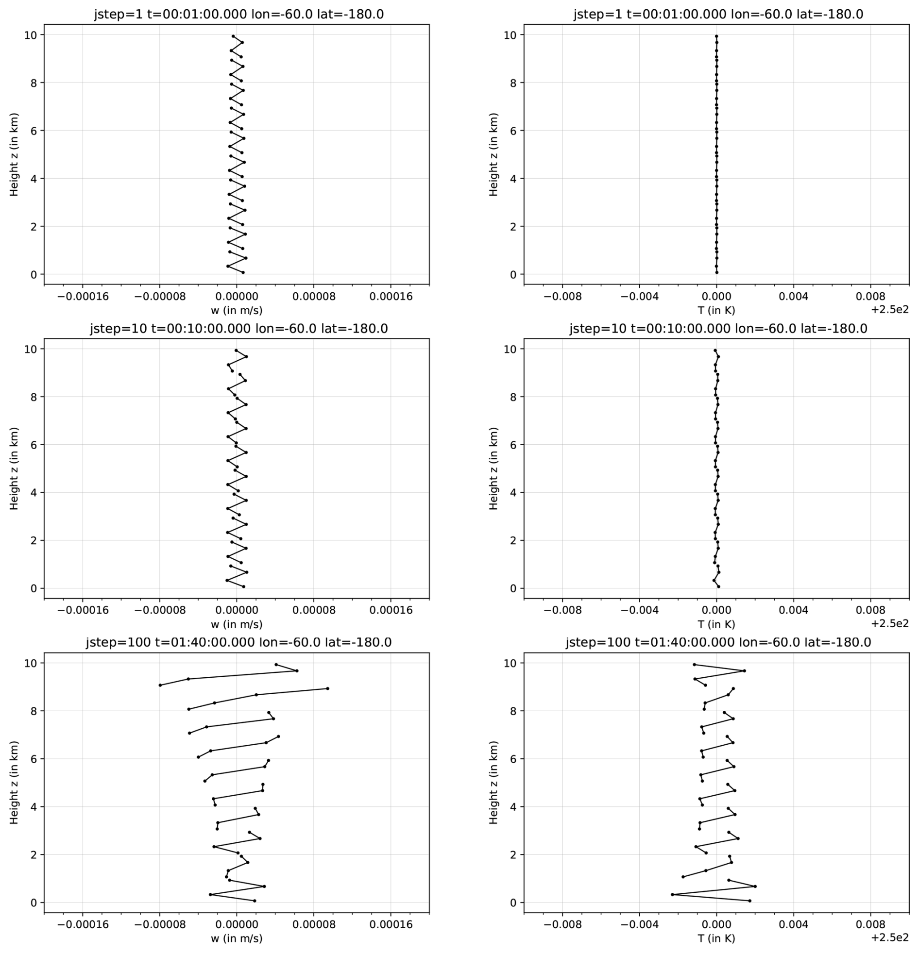
Figure 1 1D vertical Euler equations for Euler equation set “ρΘ” with 3rd degree polynomials and without source term filtering (STF). Solutions after 1, 10, and 100 time steps (top, middle, bottom row). Left: vertical velocity w, Right: temperature T. The dots denote the solution on the cell quadrature points.

In contrast, using the Euler equations with E (again first without STF) leads to simulations where w perturbations in fact tend towards 0 after several thousands of time steps. Consequently this does not lead to an increase in temperature perturbations and the simulation remains stable, at least for all considered orders 3, 4, and 5.

Running the Euler equations using E with STF has no influence on stability, and leads to quite similar results after 100 000 time steps compared to the runs without STF. However, it can lead to slightly larger amplitudes in w and T during the first time steps. In contrast, later on (after several 100 time steps) STF can lead to a quicker convergence of w towards 0.

These simulation results are in good agreement with a normal mode stability analysis given in Appendix B. The linear instability arising in the “ρΘ” system in fact can be resolved by STF over a large range of temperature stratifications. However, the equation set “E” behaves closer to the physical stability/instability behaviour, whereas the “ρΘ” set does not.

We have checked (not shown) that proper convergence is, of course, achieved in the case of stable simulations (i.e. in the case of the Euler equations using E), which means that the perturbations in w and in T are reduced by the appropriate order when reducing Δz and Δt, i.e. well-balancing problems do not violate convergence, as expected.

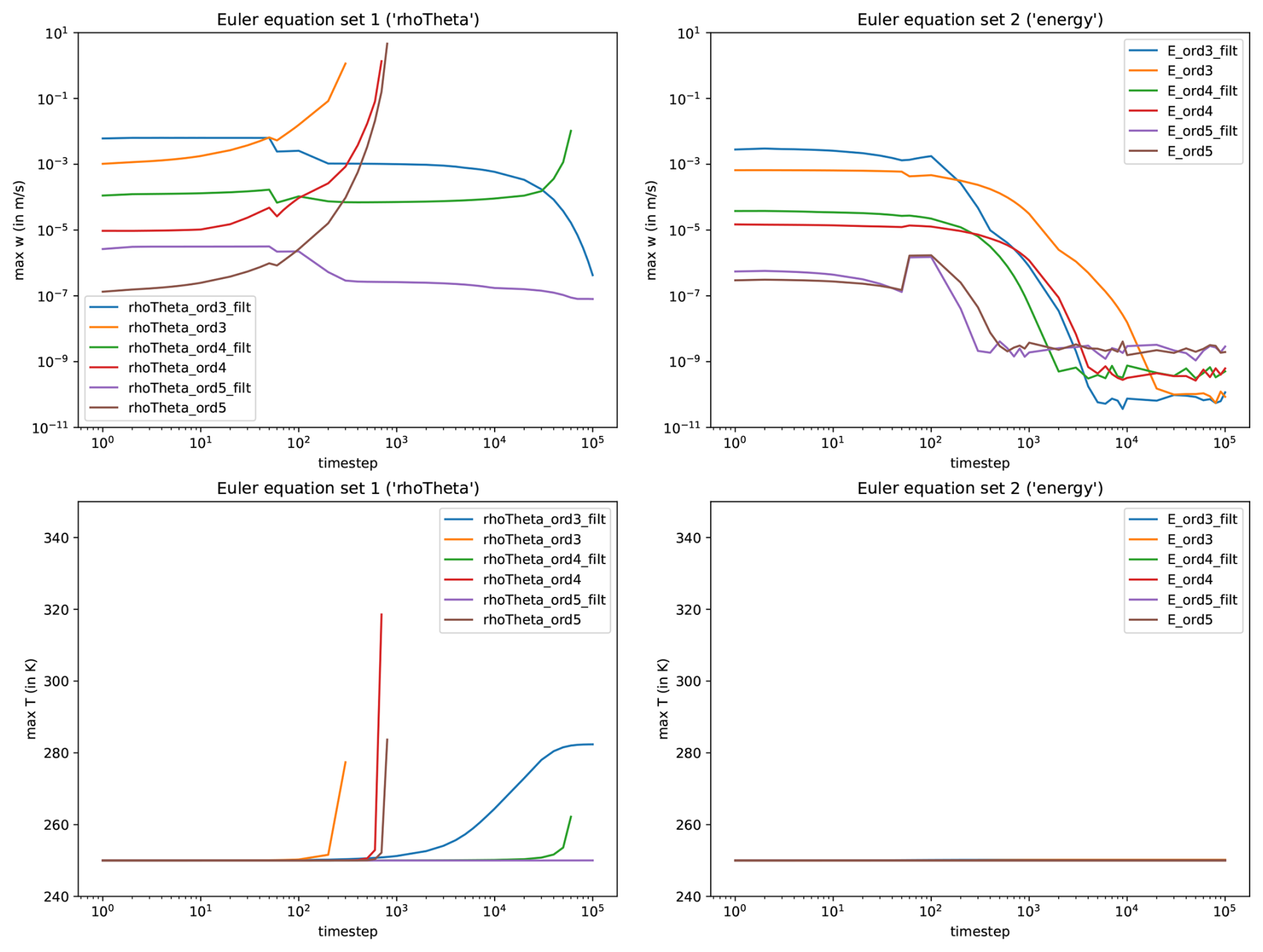
Figure 2 1D vertical Euler equations. Top: maximum absolute value of vertical velocity w over timestep, bottom: maximum value of temperature T over timestep. Left: Euler equation set “ρΘ”, Right: Euler equation set “E”. Shown are values for spatial DG order 3, 4, and 5 and with STF (lines denoted with “..._filt”) or without STF.

If not mentioned otherwise, the following simulations with equation set “ρΘ” always use STF whereas no STF is used for equation set “E”. Also we will use horizontally a 4th order (i.e. polynomial degree 3) DG spatial discretisation; this is the lowest order that reduces grid imprinting problems in shallow water equations to an acceptable level (Baldauf, 2020). Vertically we will use a 5th order scheme (i.e. polynomial degree 4). This is motivated by the results of Fig. 2, where the overall well-balancing effects are acceptably small.

6.2 Flow over mountains – linear case

To demonstrate the correctness of the terrain-following coordinate formulation, we consider a 2D flow over very low mountains on a flat plane, for which a linearised analytic solution exists (Smith, 1980, here we use the version from Baldauf, 2008). The setup is analogous to B21 (see Sect. 5.2 for details): a couple of mountains with a maximum height of 10 m are set in a stably stratified atmosphere with constant Brunt–Väisälä frequency N=0.01 s⁻¹, with constant inflow velocity of u₀=10 m s⁻¹, and without Coriolis force. We use $(\mathrm{2}\cdot \mathrm{140})\times \mathrm{16}$ grid cells (where one Δx-interval comprises two triangles, i.e. we use the quasi-2D methodology for our triangle cell stripe of Appendix A), horizontal grid spacing is Δx=1 km, the vertical grid is stretched. Figure 3 shows that the simulation of both equation sets agree quite well with the analytic solution near the ground. As it can be expected, the damping layer reduces the simulated vertical velocity near the model top. We used a time step of Δt=0.2 s for equation set “ρΘ”, whereas equation set “E” tolerates a slightly larger time step of 0.25 s (to be more precise: set “ρΘ” runs stable for Δt until 0.23 s, whereas set “E” runs stable until 0.26 s).

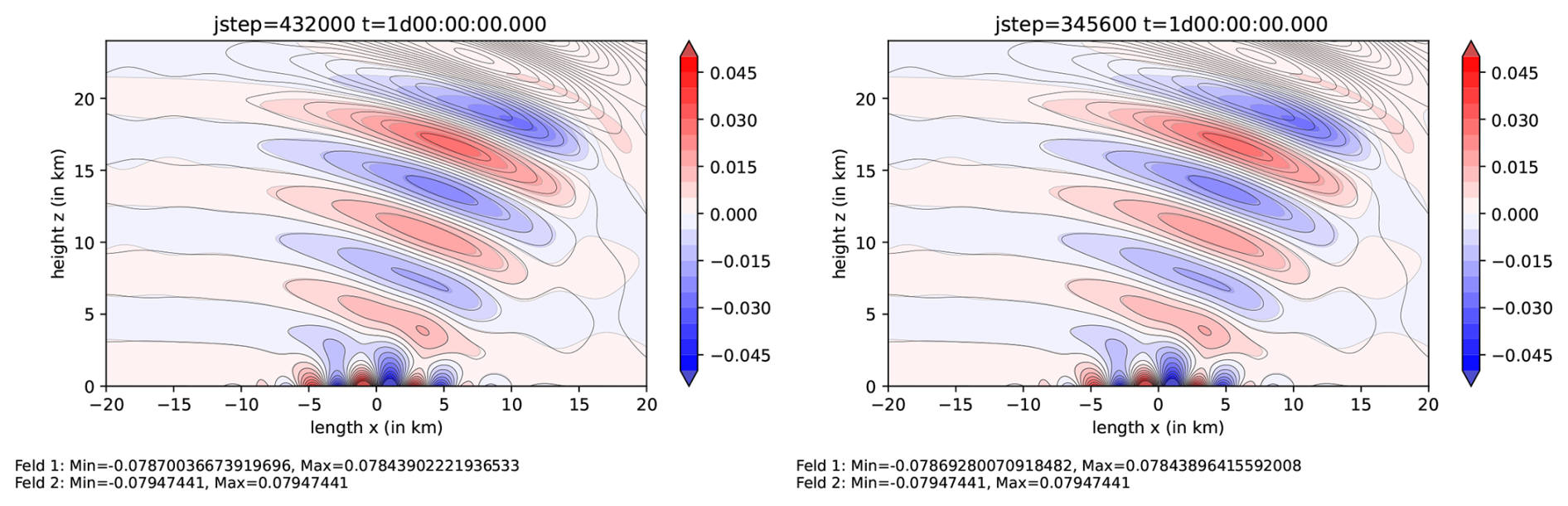
Figure 3 Linear 2D flow over mountain test. Vertical velocity $w=v^{{\mathrm{3}}^{\prime \prime }}$ after t=24 h. Black lines: analytic solution, shaded and grey, dashed lines: simulation. Left: Euler equation set “ρΘ”, Right: Euler equation set “E”.

6.3 Flow over mountains – steep case

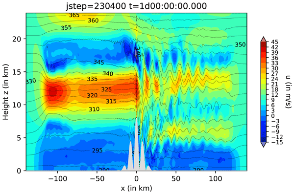
To demonstrate the quite stable behaviour of the DG method even over very steep terrain, we consider a similar test setup as in B21 (Sect. 5.5.1, see some further setup details there). A couple of mountains with a maximum height of 8 km and a very steep maximum slope angle of about 72° is set into an atmosphere with inflow velocity u=10 m s⁻¹, a stable temperature stratification with a constant Brunt–Väisälä frequency of N=0.01 s⁻¹, and without Coriolis force (Ω=0). We again use the quasi-2D methodology for our triangle cell stripe of Appendix A, with a horizontal grid spacing Δx=4 km and a vertical grid stretching. Such steep and high mountains generate a non-stationary solution due to gravity wave breaking, see Fig. 4 after 23 and 24 h of simulation time. In reality this wave breaking generates turbulence that damps it. Therefore, a simple Prandtl mixing length turbulence model (5) is used with a height-dependent (more precisely, z is the vertical distance from the bottom orography) turbulent length scale

$$l_{\mathrm{t}}={\displaystyle \frac{\mathit{\kappa }z}{\mathrm{1}+\frac{\mathit{\kappa }z}{l_{\mathrm{B}}}}},$$

where we have chosen a constant Blackadar length scale l_B=40 m and the von-Kármán-constant κ=0.4. No additional filtering was applied. We note that B21 used a Smagorinsky model, whereas here we decided for the Prandtl model since it seems to generate slightly more realistic ranges for the diffusion coefficient K_M=K_H, see Fig. 4, bottom row (negative values of K_M are an inter-/extrapolation artifact of the plotting tool, in the BRIDGE code any possible negative value is clipped away).

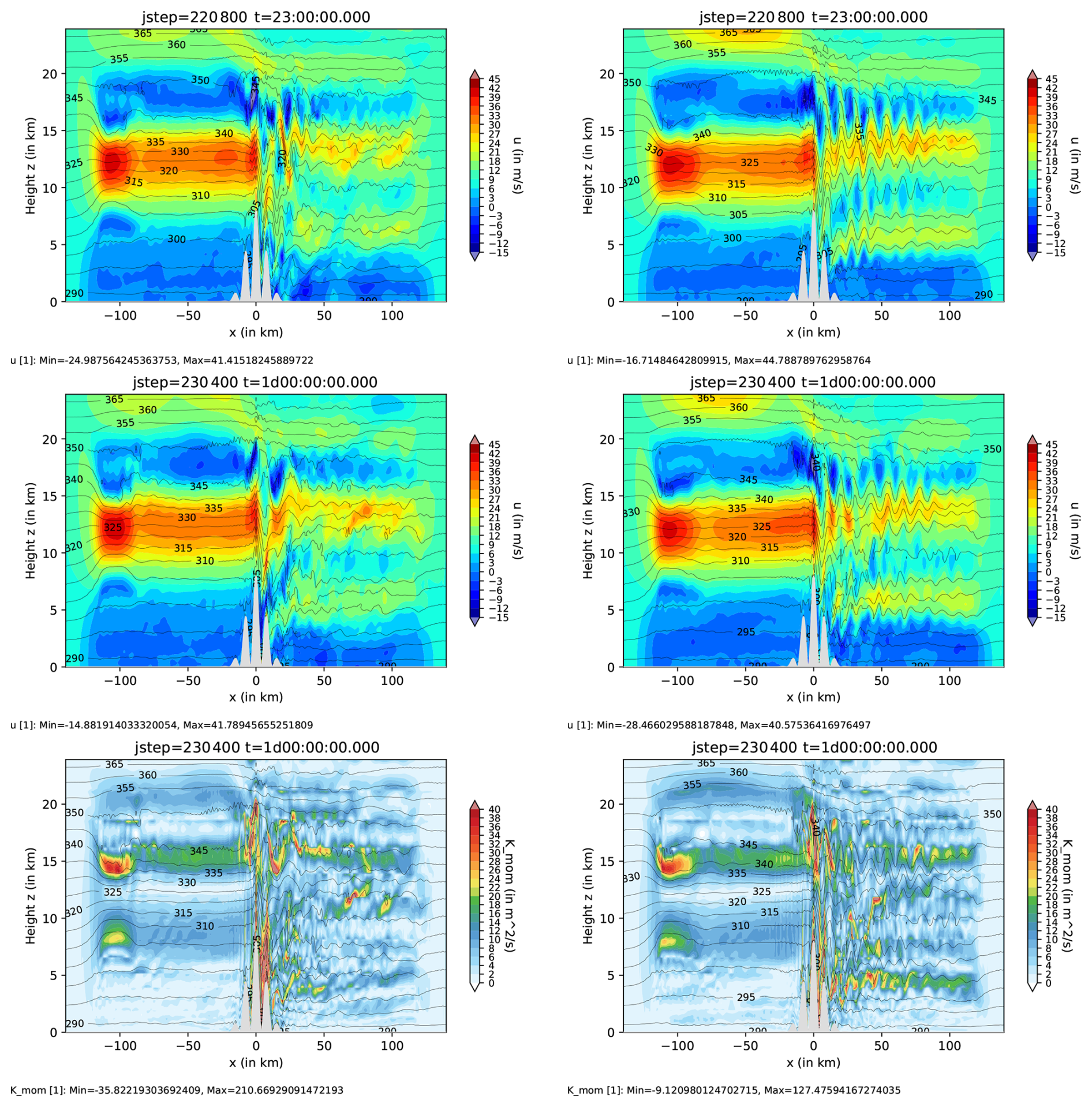
Figure 4 2D flow over steep mountains. Top: horizontal velocity component u (shaded) and potential temperature Θ (isolines) after t=23 h, middle: the same after t=24 h, bottom: diffusion coefficient K_M (shaded) and potential temperature Θ(isolines) for t=24 h. Left: Euler equation set “ρΘ”, Right: Euler equation set “E”.

Both equation sets “ρΘ” and “E” roughly show a similar qualitative behaviour (Fig. 4, left and right, respectively). The main difference is a more pronounced lee wave pattern in equation set “E”. Note that a closer similarity between both solutions cannot be expected in such a chaotic flow regime.

6.4 Density current

A strongly nonlinear 2D test case simulating a falling cold bubble was defined by Straka et al. (1993). When the bubble hits the ground and evolves in both horizontal directions, Kelvin-Helmholtz instability generates several vortices. The simulation is diffusion-limited by a constant diffusion coefficient $K_{\mathrm{M}}=K_{\mathrm{H}}=\mathrm{75}$ m² s⁻¹. The BRIDGE setup uses a grid spacing of $\mathrm{\Delta }x=\mathrm{\Delta }z=\mathrm{400}$ m (again we use the quasi-2D methodology of Appendix A), with a time step of 0.06 s using the SSP3(3,3,2) scheme for the Euler equations with diffusion terms. This results in horizontal and vertical Courant numbers of $C=(c+|v\left|\right)\frac{\mathrm{\Delta }t}{\mathrm{\Delta }{x}^i}\approx \mathrm{0.05}$. Otherwise, remarks given in B21, Sect. 5.4, about boundary conditions and details about the diffusion term also apply here. The reference state is given by Eq. (17). Figure 5 shows the potential temperature after 900 s, which for both equation sets is in a good agreement with Straka et al. (1993). Note, that our grid spacing is 16 times larger than the benchmark simulation and demonstrates the benefit of using higher order methods just for diffusion-limited flows. The total mass in the whole domain is neither increasing nor decreasing during the simulations, i.e. the jumps are below machine precision. Total energy (for the equation set “E”) in the domain is slightly increasing with a relative change of $+\mathrm{7}\times {\mathrm{10}}^{-\mathrm{14}}$ during the simulation (i.e. over 15 000 time steps). The relative changes in the domain integral of ϑ (for equation set “ρΘ”) are also below machine precision.

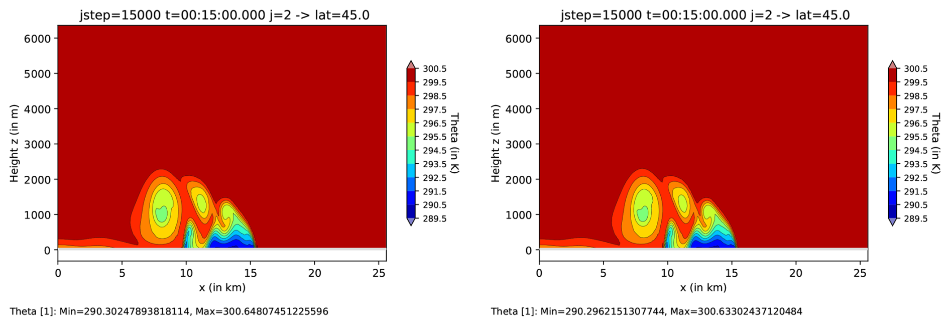
Figure 5 Density current, cold bubble test. Potential temperature Θ after 15 min. Left: Euler equation set “ρΘ”, Right: Euler equation set “E”. The contours are the same as in Fig. 1 of Straka et al. (1993).

6.5 Linear sound and gravity wave expansion on the sphere

To demonstrate the proper convergence properties of the BRIDGE code, an analytical solution is needed. Baldauf et al. (2014) present a linearised analytic solution for the compressible, non-hydrostatic Euler equations for the expansion of sound and gravity waves in a spherical shell of thickness H=10 km around a “small earth” with radius $\mathrm{6371.229}/\mathrm{50}$ km. These waves are excited by a weak warm bubble set at the north pole. The simulation is performed using various icosahedral grids with an average grid spacing of 5.681, 2.840, 1.420, 0.710°, and 3, 6, 12, 24 vertical grid cells, respectively (in the ICON nomenclature: an R2B2L3, R2B3L6, R2B4L12, R2B5L24 grid, the grid spacing is identified as the average square root of all triangle areas on the sphere). The further setup is described in Baldauf et al. (2014) for test scenario (A) with one exception: here we use a temperature perturbation ΔT=0.001 K that is smaller by a factor of 10. The reason for this is the strong reduction of errors in a 4th order DG scheme, which otherwise would exhibit visible deviations from the proper convergence due to non-linear contributions in the Euler equations. To calculate the error measures, the BRIDGE output is compared with the analytic solution on every quadrature point in the 3D spherical shell. The analytic solution itself was precalculated on a structured grid on a latitude-z-plane and is then linearly interpolated to every quadrature point (this structured grid is so highly resolved that no detrimental effect on the convergence rate by this linear interpolation is visible). Figure 6 shows error measures for vertical velocity $w=v^{{\mathrm{3}}^{\prime \prime }}$ and temperature T after 75 min of simulation time. In general, we expect 4th order convergence since we use horizontally 3rd order polynomials. Although for the time integration the only 3rd order SSP3(4,3,3) scheme was used here, we think that the time step is small enough that the overall convergence rate is determined by the spatial discretisation instead of the temporal discretization. For equation set “E” the L₁ error for w in fact shows exact 4th order convergence, whereas L₂ and even more L_∞ are not yet in their convergent regime (note that these fully 3D simulations quickly become very time consuming for higher resolutions). In contrast, equation set “ρΘ” shows much higher errors for w for coarse (vertical) resolutions than set “E”, as can be expected by the results of Sect. 6.1. This might be the reason why one seemingly sees a higher than 4th order convergence. The temperature even seems to converge in 5th order for both equation sets. We conclude that the vertical discretisation order dominates the convergence behaviour of the temperature field, in contrast to the vertical velocity field, which seems to be dominated by the horizontal convergence order.

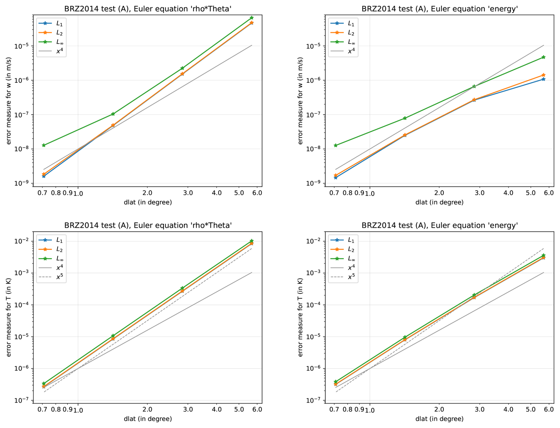
Figure 6 Linear sound/gravity wave test on the sphere, L₁, L₂, L_∞ of vertical velocity w (top) and of temperature (bottom). Left: Euler equation set “ρΘ”, Right: Euler equation set “E”. The grey, straight lines denote 4th order convergence behaviour; dashed lines denote 5th order.

Figure 7 shows a work precision diagram, i.e. the L₂ error of the vertical velocity against wall clock time, both for BRIDGE and for the ICON model (Zängl et al., 2015). All these runs have been performed on AMD EPYC 7502 32-Core Processors with 2.5 GHz (which are the current so-called login nodes at the DWD), BRIDGE mostly runs on 192 processors (384 processors for the highest resolution) and ICON on three different processor configurations for the grids R2B5L12, R2B6L24, R2B7L48. All wall clock times are converted as if running on 192 processors. In this test BRIDGE obviously outperforms ICON by far. However, this is of course due to the very smooth fields that only occur in this test case. In other words, higher order schemes necessarily must outperform the standard second order schemes in this test case.

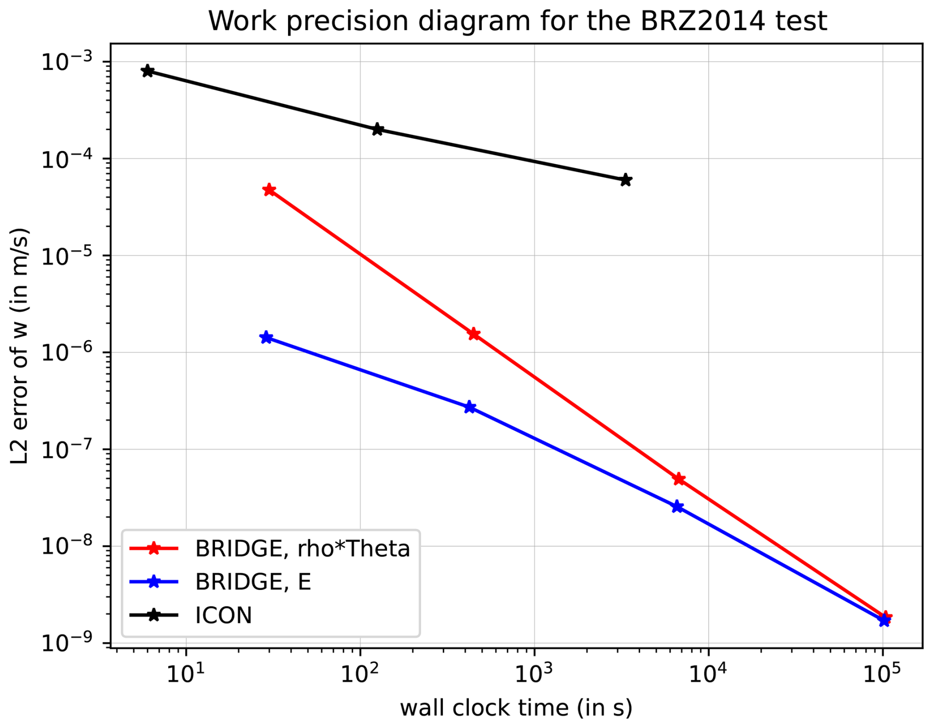
Figure 7 Work precision diagram for the linear sound and gravity wave test on the sphere: L₂ error of vertical velocity against the analytic solution vs. wall clock time. Blue line: equation set “E”, red: equation set “ρΘ”, black: ICON.

6.6 Baroclinic instability test

6.6.1 The Jablonowski, Williamson (2006) test setup

The baroclinic instability is one of the most important large-scale dynamical mechanisms in the atmosphere and to a large extent determines the weather in the mid-latitudes. Several idealized test setups have been proposed to test this phenomenon on the sphere; here we use the setup of Jablonowski and Williamson (2006): two purely zonal jet streams are analytically prescribed together with the temperature stratification in pressure coordinates (i.e. for a hydrostatic approximation of the Euler equations). To apply it for the compressible Euler equations we use the iteration procedure described in the appendix of Jablonowski and Williamson (2006). The baroclinic instability is triggered by a small perturbation in the zonal velocity component u.

One important goal in new dynamical core developments is the increase of both accuracy and efficiency (other goals are good numerical stability, and so-called mimetic properties like conservation). Therefore, as in the density current test before, one may ask, what is the coarsest possible grid spacing that is still in good agreement with the benchmark result. For a (horizontally) 4th order scheme one may expect that an about 4 times larger grid spacing can be used compared to standard second order solvers. Here, BRIDGE simulations are done for a horizontal grid with an average grid spacing of about 315 km (R2B3 grid in the ICON nomenclature). Note that this is an about 5 times larger grid spacing (i.e. a bit larger than estimated) than used by the benchmark models in Jablonowski and Williamson (2006, Fig. 7). 10 equidistant vertical levels are used until a model top of 40 km. A time step of Δt=80 s was used, which is mainly determined by the horizontal grid spacing, resulting in a Courant number of $C_x=(c+|v\left|\right)\frac{\mathrm{\Delta }t}{\mathrm{\Delta }x}\approx \mathrm{0.1}$. The linearisation coefficients of the implicit solver are updated every 10 time steps.

A first striking difference in the two Euler equation sets “ρΘ” and “E” can be seen if we apply the BRIDGE code without filtering. Figure 8 shows the meridional (north-south) velocity component v after 30 h. The simulation using equation set “ρΘ” (with STF) generates large perturbations in v that grow exponentially until a model crash after about 2.7 d. These mostly vertically oscillating perturbations seem to be an artifact of the above described well-balancing problem. In contrast, equation set “E” does not show such problems and remains stable over about 7.5 d.

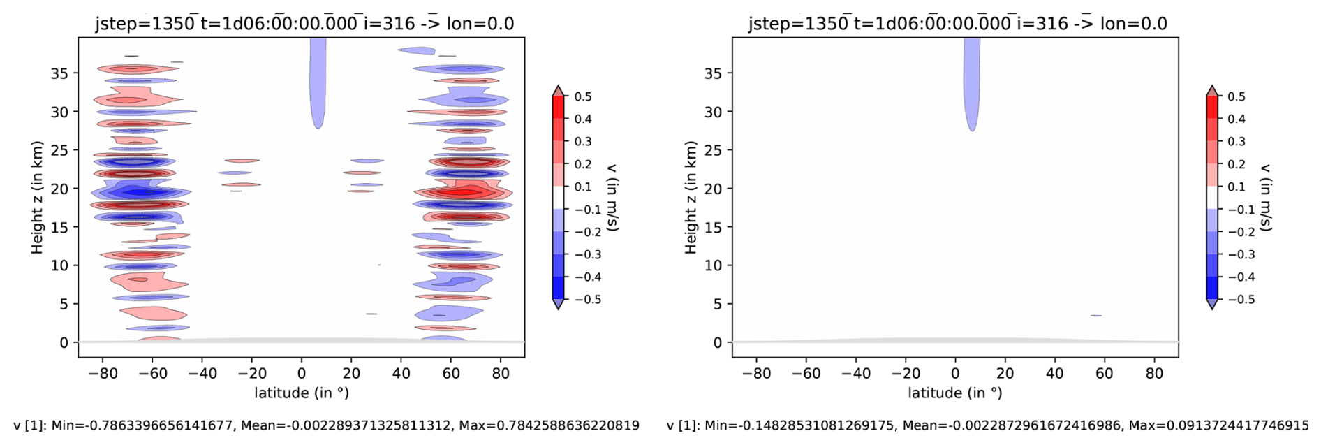
Figure 8 Baroclinic instability test, no filtering. Meridional velocity component v after t=30 h. Left: Euler equation set “ρΘ”, right: equation set “E”.

However, these results completely change if we apply filtering. We first apply a base filter with α=1.0 (horizontal) or α=0.5 (vertical), N_c=1 and 2s=10; this damps the amplitudes for the highest polynomial degree by about 5 % per timestep. Now the simulation using equation set “ρΘ” remains stable over more than 32 d and the results are quite close to what is shown in Fig. 10, left, which is in good agreement with the benchmark results of Jablonowski and Williamson (2006, Fig. 7). This demonstrates that this filter smoothing is acceptable and that the chosen grid is sufficiently fine. However, the runs with equation set “E” only gain one day more and then crash after about 8.5 d. This larger sensitivity against instabilities for set “E” is also mentioned in Reddy et al. (2023) and is explained there with its fundamental non-dissipativeness. The instability occurs at the ground where the horizontal velocity fields tend to increase in a non-physical manner.

Now we additionally apply the oscillatory sensor (based on density $\stackrel{\mathrm{̃}}{\mathit{\rho }}$) with a relatively low threshold of 0.0005. If this threshold is exceeded in a grid cell, then the stronger filter with α=0.5 (horizontal) or α=0.4 (vertical), N_c=1 and 2s=4 is applied there; this damps the amplitudes for the highest polynomial degree by about 15 % per timestep. With these filter values the simulations for both equation sets, Fig. 10, agree quite well with the benchmark results of Jablonowski and Williamson (2006, Fig. 7) for both temperature in 850 hPa and surface pressure. However, whereas the run for equation set “ρΘ” remains stable over at least 40 d, the simulation for equation set “E” breaks after about 18 d. Better stability properties of this run would require stronger filtering and therefore would reduce the accuracy. This seems to be an indication that equation set “E” suffers more from nonlinear instabilities than set “ρΘ”.

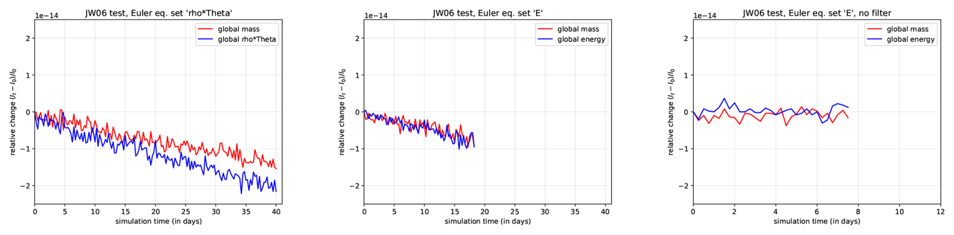
Figure 9 Baroclinic instability test, global conservation properties of mass (red) and either ρΘ or total energy (blue). Left: Euler equation set “ρΘ”, with filtering. middle: set “E”, with filtering. right: equation set “E”, without filtering.

Figure 9 shows the relative changes of globally integrated mass and either ρΘ or total energy over time, i.e. the property $(I_t-I_{\mathrm{0}})/I_{\mathrm{0}}$, where I_t is the global integral of one of these properties at time t. The relative total mass change in the whole domain is about $-\mathrm{7}\times {\mathrm{10}}^{-\mathrm{16}}$ per simulation day. The relative changes of total energy or total ρΘ are roughly in the same order of magnitude. These are quite small changes; e.g. in a 1000 year climate simulation it would mean a relative change of global mass of the order $-\mathrm{2}\times {\mathrm{10}}^{-\mathrm{10}}$, which is so small that it wouldn't be detectable by any observation in a real atmosphere. However, this result is in contradiction to the assumed local (and the resulting global) conservation property of a DG scheme mentioned in Sect. 3.2. In the right panel in Fig. 9 the filter is disabled, and in fact now there is no linear trend anymore neither in total mass nor in total energy, but only statistical noise at the roundoff limit. Therefore, we conclude that these losses do not occur due to the DG solver itself but due to tiny conservation violations of the filtering. One can speculate that these may come from roundoff errors in the Gram-Schmidt orthogonalization procedure described in Sect. 5.

The simulation took about 623 s per simulated day for both equation sets on 32 processors (2 nodes with 16 processors each) on the computer mentioned in Sect. 6.5. The simulations used $\mathrm{5120}\times \mathrm{10}=\mathrm{51}\mathrm{200}$ grid cells with $\mathrm{10}\cdot \mathrm{5}=\mathrm{50}$ base functions for each grid cell. This means 50 quadrature points in the cell and $\mathrm{3}\cdot \mathrm{4}\cdot \mathrm{5}+\mathrm{2}\cdot \mathrm{10}=\mathrm{80}$ quadrature points at all prism faces. For the 5 Euler variables this means in total $\mathrm{51200}\cdot \mathrm{50}\cdot \mathrm{5}=\mathrm{12.8}\times {\mathrm{10}}^{\mathrm{6}}$ degrees of freedom, calculated on $\mathrm{51}\mathrm{200}\cdot (\mathrm{50}+\mathrm{80})=\mathrm{6.656}\times {\mathrm{10}}^{\mathrm{6}}$ quadrature points. This wall clock time is comparable to those given for the “Finite-volume” model with comparable resolution given in Table 4 in Jablonowski and Williamson (2006) on 32 processors on an IBM power 4 architecture. However, ICON runs on the same architecture as we used a factor of about 6 faster for a similar effective resolution (a R2B5L40 grid).

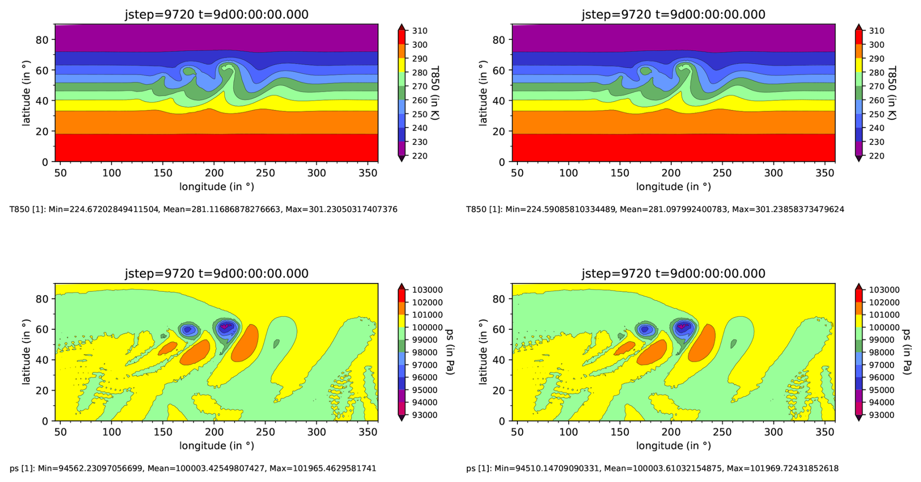
Figure 10 Baroclinic instability test, with filtering. Top: temperature T in 850 hPa at t=9 d, bottom: surface pressure p_s. Left: Euler equation set “ρΘ”, right: equation set “E”. The colors are similar to those used in Jablonowski and Williamson (2006, Fig. 7).

6.6.2 The Ullrich et al. (2014) test setup

Ullrich et al. (2014) have proposed a slightly different setup for the baroclinic instability that is based on steady analytic solutions by Staniforth and White (2011) for setting the initial state. Therefore, this setup is much easier to implement in non-hydrostatic, height based dynamical cores than the hydrostatic setup of Jablonowski and Williamson (2006). In particular, there is no need to set an orography. Therefore, we briefly show results for this test, too. The grid spacing, time step and numerical settings are the same as in Sect. 6.6.1. In particular with these filter settings the run with equation set “ρΘ” remains again stable over at least 40 d, whereas the run with equation set “E” crashes after slightly more than 11 d. Nevertheless the comparison of temperature in 850 hPa and surface pressure in Fig. 11 agree well for both equations sets with the benchmark results shown in Ullrich et al. (2014).

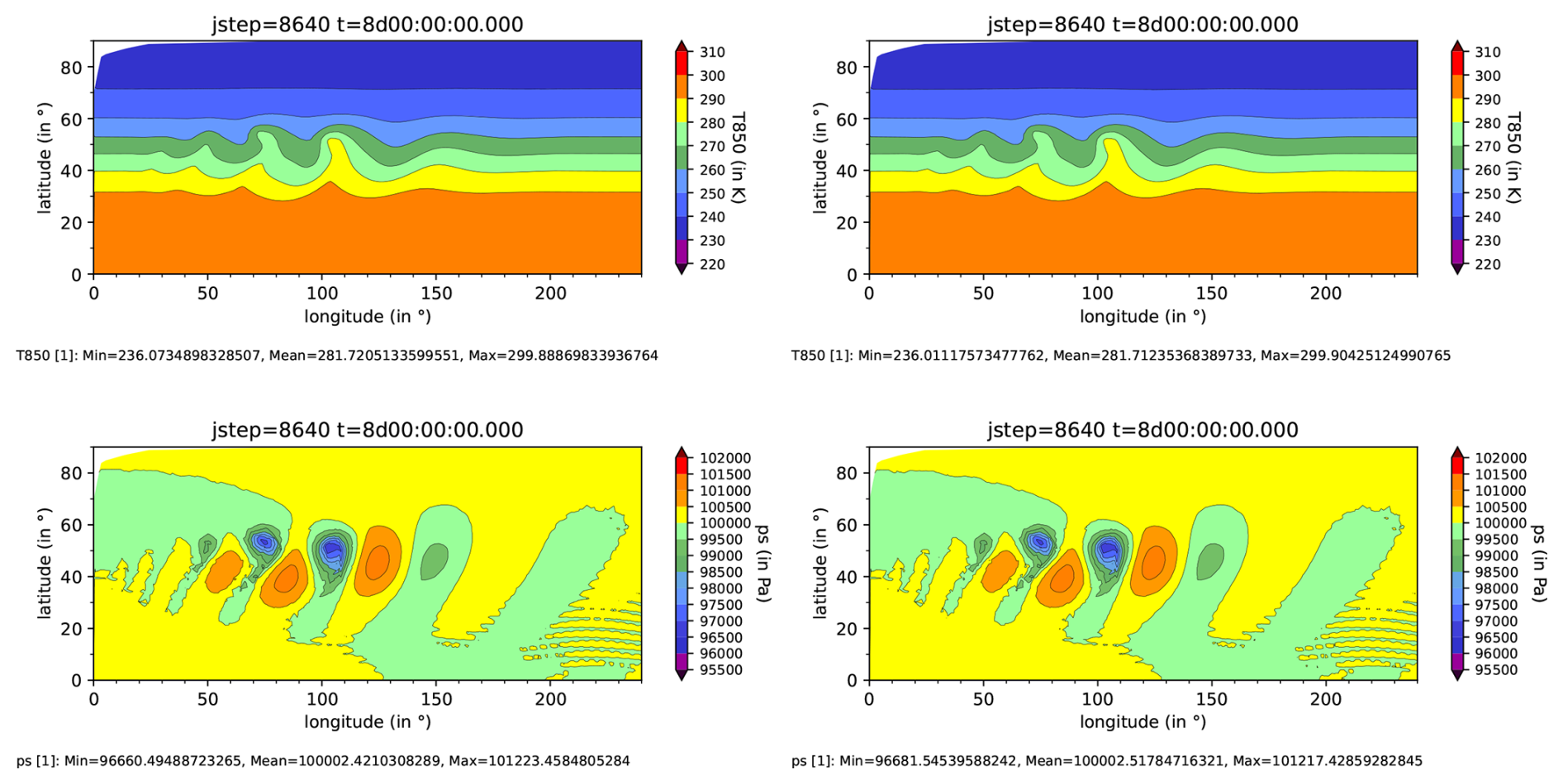
Figure 11 Baroclinic instability test by Ullrich et al. (2014), with filtering. Top: temperature T in 850 hPa at t=8 d, bottom: surface pressure p_s. Left: Euler equation set “ρΘ”, right: equation set “E”. The isolines and colors are similar to those used in Ullrich et al. (2014, Figs. 4, 5).

6.7 Simplified climate run

The Held and Suarez (1994) simplified climate run only uses the inviscid Euler equations (without moisture and without any other parameterization like turbulence or radiation) and just adds simple relaxation terms on the rhs of the equations. These terms relax towards a prescribed temperature field and the velocity back to steady state. Consequently, internal energy is supplied from outside and kinetic energy is constantly taken out in a way that resembles an averaged climate state of the earth (therefore no global energy conservation can be expected here).

Here an R2B2L8 grid, i.e. a triangle grid with about 630 km grid spacing and vertically 8 grid layers has been used. Now a vertically quadratic grid stretching was applied so that the first quadrature point is in a height of only about 32.8 m above ground (the thickness of the lowest grid cell is Δz=1060  m) and the highest quadrature point is 319.0 m below the model top of 30 km. The time step is Δt=30 s, leading to Courant numbers horizontally of $C_x=(c+|v\left|\right)\frac{\mathrm{\Delta }t}{\mathrm{\Delta }x}\approx \mathrm{0.02}$ and vertically of $C_z=\left|w\right|\frac{\mathrm{\Delta }t}{\mathrm{\Delta }z}\approx \mathrm{3}\frac{\mathrm{30}}{\mathrm{1060}}\approx \mathrm{0.1}$ (for the explicit part of the HEVI solver). We expect this value for C_z as stable with an SSP3(3,3,2) IMEX-RK scheme.

The filtering for equation set “ρΘ” is identically to what was used in Sect. 6.6. However, to run a stable simulation over 1200 d for equation set “E” a stronger base filter with values α=1.9 (horizontal) or α=1.0 (vertical), N_c=1 and 2s=10 had to be used. Additionally the update frequency of the linearisation coefficients had to be increased to every 10th time step (every 50th for equation set “ρΘ”).

Figure 12 shows the zonally and temporarily averaged zonal velocity, which can directly be compared with Fig. 2 of Held and Suarez (1994). The main structures, in particular the strengths and lateral and height positions of the two jets, are in a good agreement with this reference. However, the result for equation set “E” (right) even seems a bit closer to Fig. 5 of Souza et al. (2023), who also used the Euler equations with total energy. Slight deviations from the north-south-symmetry possibly can be traced back to the sampling strategy (note that the initial state and the relaxation fields have the full north-south-symmetry): the simulation produced output every 6 h, from which the temporary average was constructed. The relative total mass change is about $-\mathrm{2.1}\times {\mathrm{10}}^{-\mathrm{13}}$ yr⁻¹.

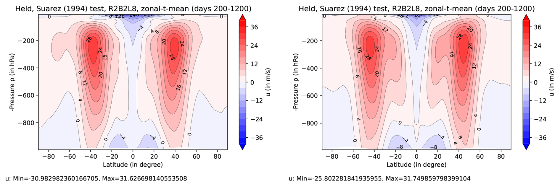
Figure 12 Simplified climate run. Zonal mean and temporal mean (over days 200 to 1200) of zonal velocity (in m s⁻¹). Left: Euler equation set “ρΘ”, Right: Euler equation set “E”. The contours are chosen as in Fig. 2 of Held and Suarez (1994).

7 Conclusions and outlook

The main goal of this article is the comparison of two Euler equation sets using density and momentum, and either density weighted potential temperature ϑ=ρΘ or total energy E as prognostic variables, both in a numerical framework of a classical DG scheme with the HEVI approach using IMEX-RK time integrators. Whereas the formulation with ϑ is mainly described in B21, here the details of a formulation with E are explained, in particular for the use in an IMEX-RK scheme. Furthermore, the combination of the HEVI approach with the local and terrain-following coordinate to treat atmospheric flows on the whole sphere are described.

One important goal of the resulting BRIDGE code is to achieve local conservation of the prognostic variables. Consequently, the use of E seems to be favourable because it especially means to fulfil the first law of thermodynamics. In contrast, although ϑ is related to entropy just under the conditions of this article, it does not mean to fulfil the second law of thermodynamics under more general conditions e.g. using moisture. In fact, some of the test cases demonstrate superior well-balancing properties of the Euler equations using E: in particular in the simple 1D vertical test, Sect. 6.1, together with the related normal mode analysis given in Appendix B and in the linear sound and gravity wave expansion test, Sect. 6.5, demonstrating lower errors in particular for coarser resolutions. In particular, no accuracy reducing STF is needed for the equation set “E”. Additionally, slight advantages could be seen in the flows over mountains – a slightly larger time step could be used in the linear flow over mountains, see Sect. 6.2, and perhaps a slightly more realistic flow pattern in the flow over steep mountains, Sect. 6.3, could be achieved (although the true solution is not known in this case).

On the other hand, the equation set “E” suffers more from non-linear instabilities than equation set “ρΘ”, seen in the baroclinic instability test in Sect. 6.6 and the simplified climate run in Sect. 6.7. This is probably a result of the non-dissipative property of an energy-conserving scheme (Reddy et al., 2023). In both cases it was harder to find a setup that runs stable for set “E”.

We want to emphasize that we only used filtering as a stabilization mechanism, mainly because this is a computationally quite cheap method. As one of its main drawbacks is the violation of well-balancing properties if applied to the atmosphere. For DG schemes there exist several other stabilizing or dealiasing techniques (for a survey see e.g. the book of Giraldo, 2020). For example, the artificial viscosity method (Persson and Peraire, 2006) is widespread. One rather technical reason for not applying it is that we did not want to use the more expensive BR1 scheme in these (essentially frictionless) test cases. Recently, hyper-diffusion has been proposed for element-based Galerkin schemes by Giraldo et al. (2024), a method that is used in many atmospheric models (like ICON). In a DG scheme the hyper-diffusion term can be incorporated in two ways. One option is to extend a scheme such as BR1 by introducing auxiliary variables for the higher-order derivatives; this approach is accurate but computationally expensive. Alternatively, the term can be added solely as a source term, which is computationally cheap but sacrifices strict conservation because the inter-cell fluxes are omitted.

Despite the somewhat mixed results for the inspected two equation systems, we will in particular continue the work on equation set “E”, due to their other positive properties described above and in the introduction. One reason for our optimism concerning numerical stability is the fact that every realistic application of an atmospheric model has to use turbulence parameterizations, which in many cases (though not generally) just perform a stabilization of the above mentioned model breakdowns. The other, more important, reason are recent developments for DG schemes towards entropy stable or even entropy conserving schemes that just build on set “E” and which have achieved a certain maturity (Gassner and Winters, 2021; Waruszewski et al., 2022). So it could be demonstrated that the baroclinic instability test of Sect. 6.6 can be run without any model breakdowns occurring and without any other stabilization measures (Waruszewski et al., 2022). Steps to extend these methods to triangles have been done by Chan (2018). However, at the moment it is less clear how to apply these new techniques to the combination of triangle grids, the HEVI approach, and the covariant formulation used in this article. In particular to the last point, recently Montoya et al. (2026) developed an entropy stable DG scheme for the covariant formulation of the shallow water equations on the sphere. We plan to follow these new developments in the near future. Such provably stable approaches even could lead to a reduction of too excessive vertical velocities, which would allow to increase the time steps (see in particular the limitation given in Sect. 6.7). We further will inspect alternative IMEX-RK schemes (e.g. those given in Giraldo et al., 2024) that might allow larger Courant numbers and therefore would lead to an improved efficiency of our BRIDGE code.

Appendix A: Quadrature rules for x-z-slice models on unit triangles

A few test cases in this article use a 2-dimensional “x-z-slice” model, i.e. we have only one horizontal direction. Since the BRIDGE code only can use triangle cells in the horizontal direction, practically, we use a stripe of squares, each square split into two triangles. Or, alternatively described, a stripe of two saw tooth rows (one upward and one downward oriented). Consequently, it is reasonable to use only 1D, x-dependent base functions in the horizontal direction for each triangle, and likewise only 1D quadrature rules. However, this requires definition of quadrature rules for only x-dependent polynomials not on a 1D interval, but on the 2D unit triangle D ($-\mathrm{1}\le x\le \mathrm{1}$, $-\mathrm{1}\le y\le -x$). This results in a Gaussian quadrature rule of the form

$$\begin{array}{}\text{(A1)}& \underset{D}{\int }{p}_n\left(x\right)\mathrm{d}x\mathrm{d}y=\sum _{i=\mathrm{1}}^N{w}_i{p}_n\left(x_i\right).\end{array}$$

To this purpose, we generate 2N equations for the first 2N monomials p_n(x)=xⁿ, $n=\mathrm{0},\mathrm{\dots },\mathrm{2}N-\mathrm{1}$ by using

$$\underset{D}{\int }{x}^n\mathrm{d}x\mathrm{d}y=\underset{-\mathrm{1}}{\overset{\mathrm{1}}{\int }}\mathrm{d}x\underset{-\mathrm{1}}{\overset{-x}{\int }}\mathrm{d}y{x}^n=\left\{\begin{array}{ll}\frac{\mathrm{2}}{n+\mathrm{1}}& n\text{ even},\\ -\frac{\mathrm{2}}{n+\mathrm{2}}& n\text{ odd}.\end{array}\right.$$

This highly nonlinear equation system for the quadrature nodes x_i and weights w_i is solved by a Newton iteration procedure. The resulting quadrature rules for different N are given in Table A1.

Table A1 Gaussian quadrature rules for only x-dependent base functions on the unit triangle.

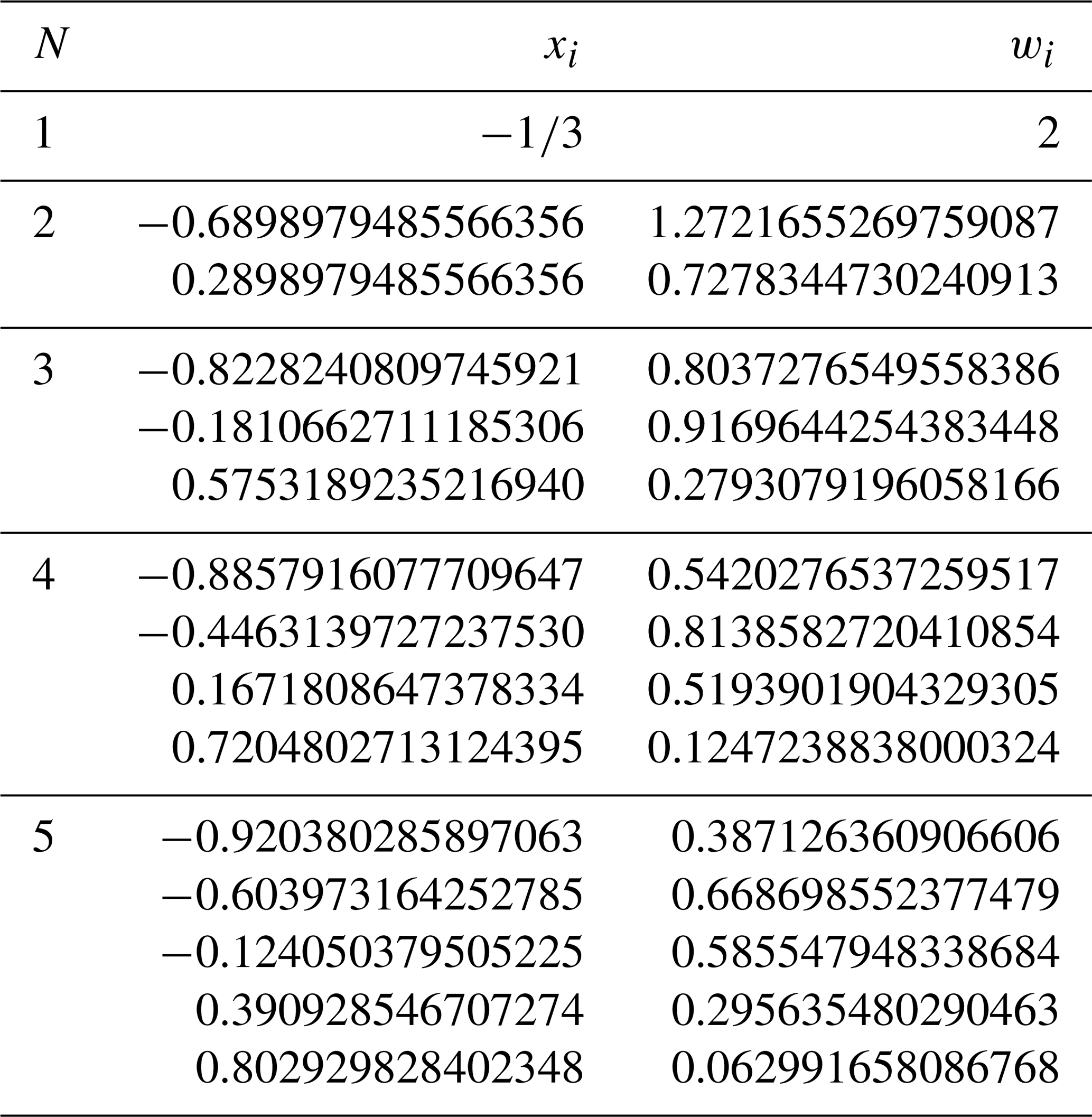
By an analogous procedure one can get Gauß-Lobatto rules for

$$\underset{D}{\int }{p}_n\left(x\right)\mathrm{d}x\mathrm{d}y=\sum _{i=\mathrm{1}}^N{w}_i{p}_n\left(x_i\right),x_{\mathrm{1}}=-\mathrm{1},x_N=+\mathrm{1}.$$

Although we have not used these in this article, for completeness the first quadrature rules for different N are given in Table A2.

Table A2 Gauß-Lobatto quadrature rules for only x-dependent base functions on the unit triangle.

Appendix B: Normal mode analysis for the 1D (vertical) Euler equations

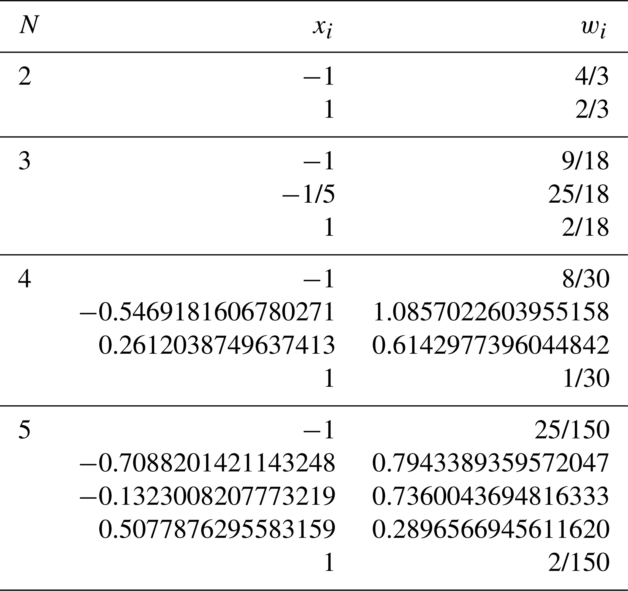
In this section the stability properties of the well-balancing issue are inspected. To this purpose we only consider one grid cell and restrict ourselves to the 1D vertical linearised Euler equations (i.e. using the linearisations in Sect. 3.1.1 and 3.1.2), without diffusion terms. So, for the equation set “ρΘ” we use

$${\displaystyle }\begin{array}{rl}& {\displaystyle \frac{\partial }{\partial t}}\left(\begin{array}{c}\stackrel{\mathrm{̃}}{\mathit{\rho }}\\ M_z\\ \stackrel{\mathrm{̃}}{\mathit{\eta }}\end{array}\right)+{\displaystyle \frac{\partial }{\partial z}}\left(\begin{array}{ccc}\mathrm{0}& \mathrm{1}& \mathrm{0}\\ \mathrm{0}& \mathrm{0}& \frac{\partial p_{\mathrm{0}}}{\partial {\mathit{\eta }}_{\mathrm{0}}}\\ \mathrm{0}& \frac{{\mathit{\eta }}_{\mathrm{0}}}{{\mathit{\rho }}_{\mathrm{0}}}& \mathrm{0}\end{array}\right)\left(\begin{array}{c}\stackrel{\mathrm{̃}}{\mathit{\rho }}\\ M_z\\ \stackrel{\mathrm{̃}}{\mathit{\eta }}\end{array}\right)\\ & =\left(\begin{array}{ccc}\mathrm{0}& \mathrm{0}& \mathrm{0}\\ -g& \mathrm{0}& \mathrm{0}\\ \mathrm{0}& \mathrm{0}& \mathrm{0}\end{array}\right)\left(\begin{array}{c}\stackrel{\mathrm{̃}}{\mathit{\rho }}\\ M_z\\ \stackrel{\mathrm{̃}}{\mathit{\eta }}\end{array}\right),\end{array}$$

and for the equation set “E”

$$\begin{array}{}\text{(B1)}& {\displaystyle }\begin{array}{rl}& {\displaystyle \frac{\partial }{\partial t}}\left(\begin{array}{c}\stackrel{\mathrm{̃}}{\mathit{\rho }}\\ M_z\\ \stackrel{\mathrm{̃}}{E}\end{array}\right)+{\displaystyle \frac{\partial }{\partial z}}\left(\begin{array}{ccc}\mathrm{0}& \mathrm{1}& \mathrm{0}\\ -\frac{R}{c_v}gz& \mathrm{0}& \frac{R}{c_v}\\ \mathrm{0}& \frac{E_{\mathrm{0}}+p_{\mathrm{0}}}{{\mathit{\rho }}_{\mathrm{0}}}& \mathrm{0}\end{array}\right)\left(\begin{array}{c}\stackrel{\mathrm{̃}}{\mathit{\rho }}\\ M_z\\ \stackrel{\mathrm{̃}}{E}\end{array}\right)\\ & =\left(\begin{array}{ccc}\mathrm{0}& \mathrm{0}& \mathrm{0}\\ -g& \mathrm{0}& \mathrm{0}\\ \mathrm{0}& \mathrm{0}& \mathrm{0}\end{array}\right)\left(\begin{array}{c}\stackrel{\mathrm{̃}}{\mathit{\rho }}\\ M_z\\ \stackrel{\mathrm{̃}}{E}\end{array}\right),\end{array}\end{array}$$

both with boundary conditions $M_z(z=\mathrm{0})=\mathrm{0}$ and $M_z(z=L)=\mathrm{0}$.

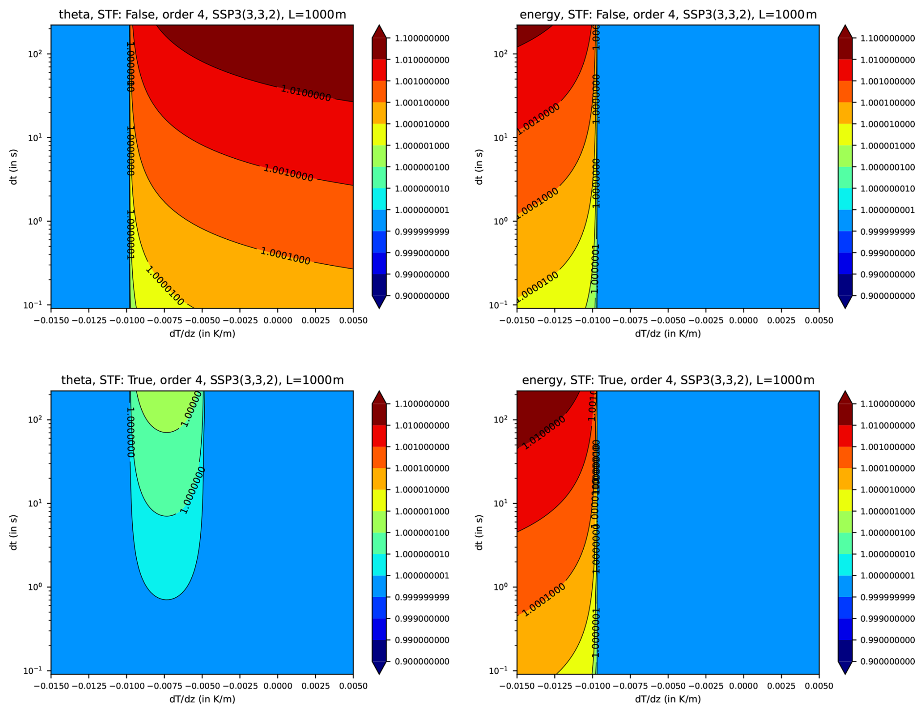
Figure B1 Maximum amplification factor for the 1D vertical stability problem. Left: Euler equation set “ρΘ”, Right: Euler equation set “E”. Top: without STF, Bottom: with STF.

In contrast to a von-Neumann-stability analysis, a normal mode analysis can treat linear equations with non-constant coefficients, too, e.g. vertically varying density, pressure or temperature. Therefore we can also inspect different temperature stratifications that we prescribe by a polytropic atmosphere of the form $T\left(z\right)=T_{\mathrm{0}}+\frac{\mathrm{d}T}{\mathrm{d}z}z$. In Fig. B1 the maximum amplification factors of both equation sets with or without source term filtering (STF) is shown over the stratification $\frac{\mathrm{d}T}{\mathrm{d}z}$ and over the time step. The maximum amplification factor is calculated as the maximum eigenvalue of the 12×12 amplification matrix for a 4th order DG scheme together with an SSP3(3,3,2) IMEX scheme (all above terms are treated with the implicit part) and a grid spacing of Δz=1000 m. Note that the atmosphere becomes physically unstable for $\frac{\mathrm{d}T}{\mathrm{d}z}<-g/c_p\approx -\mathrm{0.01}$ K m⁻¹. We see that the equation set “E” behaves in a reasonable way: it is stable (the maximum amplification factor is equal to one) for the physically stable range and unstable for the physically unstable range. This is quite independent on the use of STF, so we don't need STF for equation set “E”. In contrast, the equation set “ρΘ” without STF is only stable in the physically unstable range and unstable in the physically stable range. Although the numerical instability is quite slow for moderate time steps (amplification factors are only slightly larger than one), it can nevertheless produce a problematic behaviour in longer simulation runs. STF resolves the numerical instability, with the exception of a very weak instability for larger time steps and $\frac{\mathrm{d}T}{\mathrm{d}z}<-\mathrm{0.005}$ K m⁻¹.