
the Creative Commons Attribution 4.0 License.
the Creative Commons Attribution 4.0 License.
 | 17 Jul 2026
A high-resolution urban CO2 transport model with anthropogenic and biogenic fluxes
Jie Zheng
Fangxin Fang
We develop PALM-CO2, a high-resolution urban carbon dioxide transport model with anthropogenic and biogenic carbon emissions. The PALM-CO2 model is implemented within the open-source urban-flow large-eddy simulation (LES) model PALM. Anthropogenic CO2 emissions are prescribed using an external emission inventory, while biogenic CO2 fluxes are computed online using the Vegetation Photosynthesis and Respiration Model (VPRM). In addition, custom output modules are developed to diagnose carbon fluxes. PALM-CO2 is validated through a case study in London, comprising an 8 by 8 km2 domain covering the borough of Camden at a resolution of 10 m. Simulations are driven by reanalysis meteorological forcing and background CO2 concentrations, while the hourly anthropogenic emissions at 10 m resolution are explicitly derived in this study. Validation against eddy-covariance flux measurements within the study region confirms that the model captures the diurnal variation of turbulent transport and anthropogenic emissions. The biogenic flux module is evaluated independently using observed monthly diurnal profiles of biogenic CO2 fluxes from a deciduous forest site in the Czech Republic. The comparison shows that the model captures realistic seasonal and diurnal variations in ecosystem carbon exchange. Analysis of the London simulations reveals strong spatial heterogeneity in near-surface CO2 concentrations arising from the interaction of building-induced turbulence, diurnal boundary-layer evolution, and emission patterns. PALM-CO2 provides a high-resolution framework for investigating CO2 transport processes in complex urban and vegetated environments, providing improved quantification of urban emission sources.
- Article
(20913 KB) - Full-text XML
- BibTeX
- EndNote


Greenhouse Gas (GHG) emissions cause global climate change, with carbon dioxide (CO2) being the most significant contributor (Intergovernmental Panel on Climate Change, 2023). To understand the impact of CO2 emissions, physical models have been used for modelling the carbon cycle and climate. The Coupled Model Intercomparison Project (CMIP) (Anav et al., 2013) compares 18 earth system models' ability to simulate the global carbon cycle across land and ocean; the models provide important insights for stakeholders, for example, climate projections from these models are used in Intergovernmental Panel on Climate Change (IPCC) report.
In the global carbon budget (Friedlingstein et al., 2023) for 2013–2022, anthropogenic activities (fossil CO2 and land-use change) account for 12.9 GtC per year, while land uptake is 3.3 GtC per year and ocean uptake is 2.8 GtC per year. The numbers show the imbalance of the emission caused by anthropogenic activities and the huge uptake provided by biospheres and natural processes. Accurately representing both anthropogenic emissions and biospheric CO2 fluxes is therefore essential for reliable carbon dioxide modelling.
A large portion of emissions occurs in urban environments (Dhakal, 2010; Marcotullio et al., 2013) due to industrialisation and high population density – the energy sector produces 40 %–80 % of global energy-related carbon emissions. Urban environments exhibit strong spatial and temporal heterogeneity in emissions as a result of diverse land use, building topography, and socioeconomic activities, leading to complex intra-urban emission patterns. For example, Christen et al. (2011) estimated carbon emissions for a Vancouver neighbourhood at a 50 m grid resolution using activity data from buildings, waste, and transportation, demonstrating how heterogeneous urban land use influences emission patterns. Smith et al. (2025) adopted land-use regression to model carbon dioxide mixing ratios in the San Francisco Bay Area, showing the great intra-urban variance of carbon emission patterns. These studies have indicated the complexity in spatial and temporal patterns of anthropogenic emissions.
For urban carbon transport modelling, anthropogenic emission inputs are typically derived from inventories at kilometre-scale or coarser resolution and must be spatially disaggregated to match the model grid. This downscaling process commonly employs surrogate variables such as population density, building data, traffic activity, and land-use. While the methodology for generating fine-scale emission maps is acknowledged, their implementation depends strongly on the availability of local activity and geospatial datasets. Several urban inventories have achieved resolutions from 1 km down to 50 m by integrating activity data and remote sensing products (London Datastore, 2023; Christen et al., 2011; Järvi et al., 2019; Cai et al., 2023). However, 10 m resolution anthropogenic CO2 emission datasets suitable for large-eddy simulation applications remain scarce. This is a critical limitation, as coarse-resolution inventories cannot resolve the strong spatial heterogeneity of urban emissions, leading to biased or overly smoothed surface flux representations at neighbourhood scales.
In addition to anthropogenic emission, biogenic fluxes can serve as a source or sink for atmospheric CO2 (Friedlingstein et al., 2023). The land biosphere and oceans together currently act as a net sink of anthropogenic CO2, absorbing about half of human emissions each year (Friedlingstein et al., 2023). However, on the urban scale, the diurnal cycle of biosphere activities yields temporally varying biogenic fluxes. To represent these processes, biogenic carbon models have been developed that explicitly simulate the underlying biochemical mechanisms of vegetation photosynthesis and ecosystem respiration. For example, Gerbig and Koch (2024) applied the Vegetation Photosynthesis and Respiration Model (VPRM, Mahadevan et al., 2008) to calculate biosphere-atmosphere exchange fluxes for CO2 across Europe. At the urban scale, Järvi et al. (2019) introduced a new biogenic carbon model that accounts for both human metabolism and vegetation effects, while Stagakis et al. (2025) conducted an intercomparison of four different biogenic models, highlighting discrepancies between model formulations. These studies demonstrate that biogenic fluxes can substantially influence urban CO2 budgets, yet their integration with high-resolution transport models remains limited.
To investigate the transport of atmospheric components, physically based urban flow models have been developed to resolve local meteorological conditions. These models are grounded in physical principles and solved numerically, enabling simulations at very fine spatial-temporal resolutions. The models have been widely used to study heatwave (Anders and Maronga, 2025) and pollution episodes (An et al., 2007), and local micro-climate's impacts on, for example, building energy usage (Pfafferott et al., 2021) and safety operations of air vehicles (Jiang et al., 2024) as well as urban ecosystems (e.g. vegetation degradation (Neves et al., 2018)). Such models generally take consideration of local urban topology including terrain height and building geometries, land and vegetation types, meteorological driving forces (e.g. wind and radiation), as well as anthropogenic activities (e.g. chemical emissions and heat fluxes). Examples of such models are PALM (Maronga et al., 2020) and DALES (Heus et al., 2010).
Beyond advancing the understanding of physical mechanisms, finer-resolution carbon transport models in urban environments are essential for accurately representing concentration fields, thereby improving the model’s capability to infer urban emission sources from ground-based measurements. This has been widely acknowledged within air pollution studies, as fine-resolution modelling enhances exposure assessment and supports source attribution and mitigation strategies (Stroh et al., 2007; Li et al., 2016; Fenech et al., 2018). In contrast, such approaches are less commonly applied in the CO2 study. For example, Brunner et al. (2019) demonstrated that neglecting realistic vertical emission profiles can lead to substantial overestimation of near surface CO2 concentrations by up to 14 % in summer and 43 % in winter – highlighting the importance of vertical resolution in modelling. The limited use of fine scale CO2 transport modelling in urban environments may partly stem from the scarcity of dense observational datasets. This gap motivates the development of integrated, high-resolution modelling frameworks that consistently couple urban flow dynamics with both high spatial resolution anthropogenic CO2 emission datasets and biogenic CO2 fluxes.
In this study, we develop an urban CO2 transport modelling framework (PALM-CO21) with 10 m resolution in both the horizontal and vertical directions, coupled with a CO2 emission inventory resolved at the same spatial scale. The model is built upon the PALM large eddy simulation (LES) system (Maronga et al., 2020), which provides an accurate representation of urban scale flows and turbulence. Within this framework, we implement a biogenic CO2 flux module and incorporate anthropogenic emission inventories as external inputs, enabling the simultaneous simulation of transport processes and surface–atmosphere CO2 exchange in complex urban environments.
A key component of this work is the development of a new 10 m anthropogenic CO2 emission inventory derived from an existing 1 km inventory using multiple spatial proxies. This high-resolution inventory is combined with high-resolution biogenic CO2 fluxes and implemented as spatially and temporally varying surface scalar fluxes within the PALM LES framework. The resulting modelling system enables the representation of neighbourhood-scale variability in both anthropogenic emissions and biogenic uptake, which cannot be captured using coarse-resolution inventories alone.
To support urban-scale applications, we design a dedicated workflow to spatially disaggregate anthropogenic CO2 emissions for the study area of London. This workflow generates a high resolution emission grid map at 10 m × 10 m resolution by integrating multiple sources of locally available urban geoinformation, including residential and commercial property datasets, gas consumption statistics, industrial point-source inventories, and detailed road network maps. These datasets are combined to apportion emissions consistently across urban surface types and activity sectors, ensuring compatibility with the PALM computational grid.
Model performance is evaluated against eddy-covariance measurements within the study area. The results show that PALM-CO2 reproduces the observed diurnal variability of turbulent CO2 transport and anthropogenic emission signals. The biogenic flux module is evaluated independently using observed monthly diurnal CO2 fluxes from a deciduous forest site in the Czech Republic, demonstrating its ability to capture realistic seasonal and diurnal patterns of ecosystem carbon exchange.
The London simulations reveal pronounced spatial heterogeneity in near-surface CO2 concentrations arising from the combined effects of urban morphology, building-induced turbulence, boundary-layer evolution, and spatially varying emission sources. PALM-CO2 provides a high-resolution framework for investigating urban CO2 transport and surface-atmosphere exchange processes and offers new opportunities for urban carbon monitoring, source attribution, and future emission inversion studies.
PALM-CO2 is implemented within the PALM model system (Maronga et al., 2020), a large-eddy simulation (LES) framework designed for high-resolution simulations of atmospheric flow in complex urban environments. PALM explicitly resolves the dominant turbulent eddies while parameterizing subgrid-scale (SGS) motions, and provides a modular structure that supports detailed representations of urban topography, land–atmosphere interactions, and scalar transport. Building upon these capabilities, PALM-CO2 extends the existing trace-gas functionality of PALM to enable the simulation of urban-scale CO2 transport coupled with spatially and temporally resolved surface fluxes.
2.1 PALM framework and LES formulation
In PALM, the transport of passive scalar quantities, including trace gases, is governed by the filtered scalar conservation equation (Maronga et al., 2020):
where s is the concentration of the trace gas in kg m−3, t is time, ρ is the density of dry air, uj is the jth component of velocity, xj is the spatial coordinate, and χs is the source or sink term of the passive scalar. Variables with double prime (′′) refer to the subgrid-scale (SGS) component of the corresponding variables, while the over-bar indicates the filtered quantities. The advection and SGS turbulent flux divergence terms are discretized using finite-difference schemes implemented in PALM, and SGS fluxes are parametrised via an eddy-diffusivity approach consistent with the LES formulation.
PALM-CO2 leverages these existing scalar transport codes and augments them with dedicated modules to represent anthropogenic and biogenic CO2 fluxes. These fluxes enter the scalar transport equation exclusively through the source or sink term χs, ensuring a clean separation between atmospheric transport processes and surface exchange parametrisations.
Figure 1 illustrates the overall structure of PALM-CO2, including the coupling between the flow solver, the biogenic flux module, and the prescribed anthropogenic emission inputs.
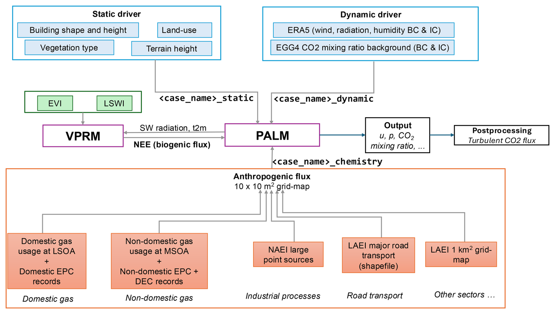
Figure 1Schematic workflow of the PALM–VPRM modelling system. Blue boxes indicate static and dynamic drivers, green boxes indicate VPRM-related vegetation inputs, purple boxes denote model components, orange boxes represent anthropogenic emissions inputs, and black boxes indicate model outputs and post-processing. Arrows show the direction of data exchange and processing. Input files are indicated in a monospace font.
2.2 Biogenic flux model
Biogenic CO2 exchange is represented using the Vegetation Photosynthesis and Respiration Model (VPRM; Mahadevan et al., 2008), which parametrises the ecosystem-scale carbon uptake and release based on vegetation state and meteorological drivers. VPRM has been widely applied in regional and urban-scale carbon studies (Ahmadov et al., 2007, 2009; Pillai et al., 2010, 2011). The parameters in the VPRM model are typically fitted using measurements from local eddy-covariance flux towers. In this study, we select a set of parameters (see Appendix F) from the WRF-Chem module (Skamarock et al., 2019) that has been calibrated using flux tower measurement in Europe (Lian et al., 2021).
In PALM-CO2, VPRM computes gross primary production (GPP) and ecosystem respiration (RESP) using the following equations:
where λ is a parameter fitted with the measurement of biogenic fluxes. Vegetation status and water stress are represented by the Enhanced Vegetation Index (EVI) and the Land Surface Water Index (LSWI). Pscale is a coefficient accounting for the degree of leafiness which is computed from LSWI and also depends on EVI to determine whether the vegetation has reached full leaf expansion,
THleaf full expansion is a threshold for vegetation growing cycle. EVI above the threshold means the growing period between leaf full expansion and senescence and below the threshold is during bud burst to leaf full expansion and during senescence. The threshold is computed from the annual maximum and minimum EVI for the computation grid,
Wscale accounts for the water content in the vegetation and is computed from LSWI,
PAR is photosynthetically active radiation which is correlated with short-wave (SW) radiation: ; PAR0 is a parameter for half photosynthetic saturation. Tscale is a coefficient computed from air temperature T,
with Tmin, Topt, and Tmax denoting minimum, optimal, and maximum temperatures for photosynthesis. Tair is the air temperature.
The respiration flux is mainly determined by the air temperature Tair and is computed from
where α and β are coefficients that vary among different vegetation types. The net ecosystem exchange (biogenic flux) is then calculated
where a negative value means net uptake and a positive value means net emission.
2.3 Diagnostic turbulent CO2 fluxes
To facilitate comparison with eddy-covariance observations and to analyse vertical CO2 exchange, PALM-CO2 includes a diagnostic computation of turbulent scalar fluxes. The vertical turbulent flux (F) is defined as
where angle brackets denote the temporal average,
where τ is the time window for averaging. w′ and s′ are the deviations from the mean of the vertical velocity component and tracer gas concentration (e.g. CO2) respectively,
Then the flux can be computed from the following temporal averaged quantities,
In the last line, the spatially filtered quantities and and their product from the Large-eddy simulation (LES) code are used to compute the vertical turbulent flux for the CO2 concentration. A major assumption is the omission of the sub-grid scale turbulent flux, which requires the grid size to be small enough to resolve the total turbulent flux. It is shown in the grid sensitivity study (Sect. 4.4) that the resolved flux at medium height boundary layer (higher than three roughness-layer heights) takes over 96 % of the total turbulent flux. Thus, the assumption is valid. A minor assumption is that the spatial filtering and time averaging commute and that the filter preserves the mean, such as . This assumption requires the averaging window is long enough to converge the statistics at all spatial locations. A computation of eddy turnover time (about 450 s for the grid sensitivity study case) shows that a half-hour average window (1800 s) covers about four eddy turnover periods, validating this minor assumption. The temporal averaging of is added to the code via a user-defined procedure. Its rolling sum is computed during time-stepping in the code, and its temporal average 〈ws〉 is computed and reported after each averaging time window τ. 〈w〉 and 〈s〉 can be easily recorded using the default output settings in PALM. The time window for averaging is set as 0.5 h.
2.4 Anthropogenic emission representation and disaggregation methodology
Anthropogenic CO2 emissions for urban areas are commonly provided as coarse-resolution inventories, typically with a kilometre-scale spatial resolution, and as annual totals. For use in high-resolution urban transport models, such inventories must be disaggregated both spatially and temporally to match the computational grid and time step. A direct interpolation of coarse grid values onto a fine-resolution model grid is straightforward but insufficient to represent realistic urban emission patterns, which are often dominated by localised sources such as building heating systems, traffic corridors, and industrial point sources. The method for processing emission inputs for chemistry transport models has been implemented in several existing tools, including the online emission module in COSMO (Jähn et al., 2020) and the stand-alone processors HERMES (Guevara et al., 2019), EMIPS (Chen et al., 2023), and FUME (Belda et al., 2024). However, these tools are primarily designed for global and regional applications and directly use emission inventories at those scales; therefore, they are not readily applicable to our study.
To address this, a sector-based disaggregation strategy is adopted. Disaggregation is applied on the sub-subsection levels defined in the LAEI dataset (London Datastore, 2023, listed in Appendix A). Emission sub-subsectors contributing only a small fraction of total emissions are distributed uniformly in space and time after interpolation to the fine grid. In contrast, dominant sub-subsectors are spatially disaggregated using additional geospatial surrogate data that represent the underlying emission-generating activities. This approach balances accuracy with data availability, as comprehensive surrogate datasets are not uniformly available for all emission sub-subsectors. The selection of sub-subsectors for detailed disaggregation is therefore based on their relative contribution to total emissions.
For sub-subsectors selected for fine-scale treatment, spatial disaggregation relies on auxiliary geospatial datasets such as building-level energy information, industrial point-source inventories, and road network data. These datasets are used as spatial proxies to redistribute emissions from coarse administrative or grid-based units to individual buildings, road segments, or point sources, which are then aggregated to the target model grid resolution.
Temporal disaggregation is applied to convert annual emissions into hourly fluxes. Sub-subsector-specific temporal profiles are used where available, capturing diurnal, weekly, and seasonal variability in anthropogenic activities. Sub-subsectors with negligible contributions are assigned constant temporal profiles, while dominant sub-subsectors employ time-varying profiles derived from established emission databases.
2.5 Implementation of PALM-CO2 framework
PALM provides an interface for user-defined chemical mechanisms where one can set up the chemical components (Khan et al., 2021). In PALM-CO2, CO2 is represented as a single passive scalar without chemical reactions. Both anthropogenic and biogenic fluxes are treated as surface source terms and are incorporated into the scalar transport equation through χs in Eq. (1).
Biogenic CO2 fluxes are computed by VPRM, whereas anthropogenic emissions are provided as externally prepared, time-resolved gridded datasets. VPRM (described in Sect. 2.2) is implemented in PALM as part of an online chemistry module, where biogenic fluxes are computed prior to solving the scalar transport equation using near-surface air temperature and short-wave radiation retrieved from PALM runtime variables. Anthropogenic emission sources (described in Sect. 3.2) are supplied as hourly NetCDF files, requiring activation of the level-of-detail (LOD) 2 option in PALM.
Both biogenic and anthropogenic fluxes are prescribed as source terms in the lowest atmospheric grid cell adjacent to the surface. In locations where complex terrain or building structures elevate the first fluid grid cell above ground level, the surface fluxes are applied at that elevated cell. This approach maintains a physically consistent coupling between surface emissions and the resolved airflow, ensuring that fluxes are introduced directly into the urban canopy layer where turbulent exchange and transport are explicitly represented.
3.1 Study area
A study area in London was selected for model validation and analysis, as shown in Fig. 2. London is selected for its high population density, high level of urbanisation, and its vast amount of green infrastructures. In Camden, there is a CO2 flux measurement station located at 190 m height on the BT tower (Helfter et al., 2011, 2016), providing an independent dataset for evaluating the performance of the model developed in this study.
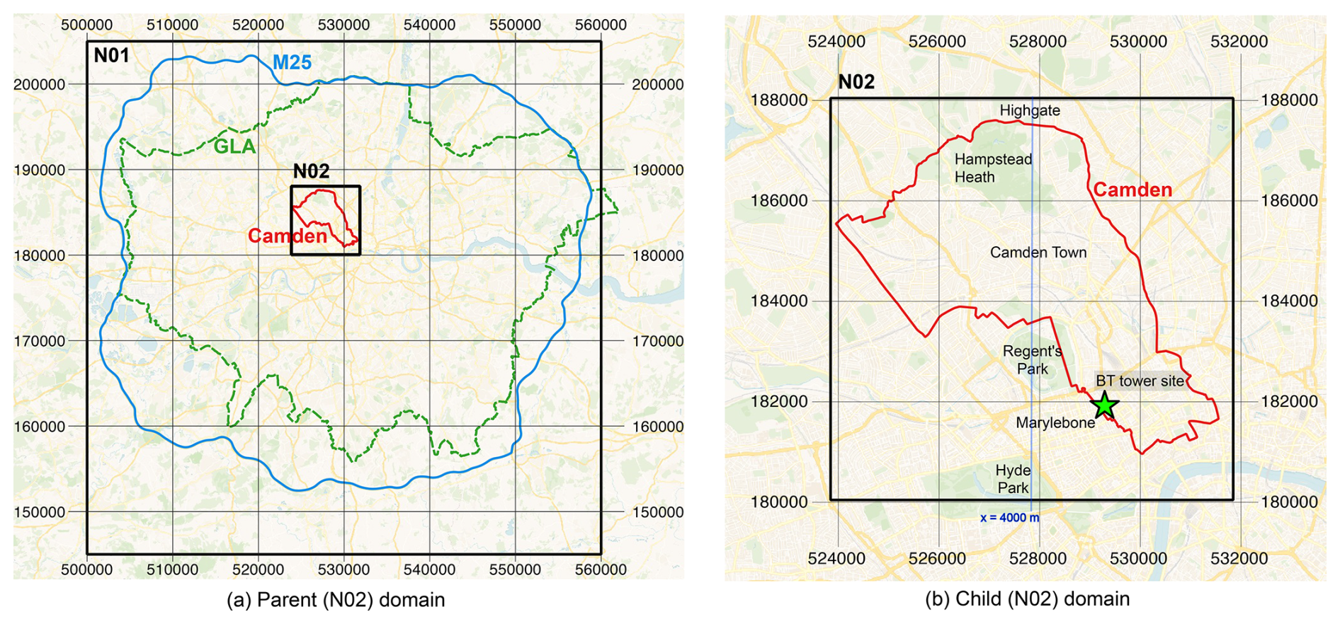
Figure 2A nested study area surrounding M25 motorway and London Borough of Camden. Coordinates are in British National Grid coordinate system. (a) The parent domain (denoted as N01) is roughly surrounding M25 motorway and the Greater London Area (GLA); the domain size is 60 km by 60 km. (b) The child domain (denoted as N02) encompasses Camden and its size is 8 km by 8 km. A measurement site (BT tower) is marked with a green star in the child domain. A x=4000 m line where the vertical cross-section data is extracted for analysis is shown in blue; the origin of the N02 domain is the bottom-left corner. Map data in the figure are from OpenStreetMap (© OpenStreetMap Distributed under the Open Data Commons Open Database License (ODbL) v1.0 (for further information, please see OpenStreetMap)).
The Greater London Authority (GLA) area (Fig. 2a) is characterised by a highly heterogeneous land-use and urban landscape. At its core lies a dense, multifunctional urban structure dominated by commercial, financial, and high-density residential uses, with extensive transport infrastructure and limited open space. Moving outward, land use transitions to predominantly residential neighbourhoods of medium to low density, interspersed with local centres, industrial estates, and major road and rail corridors. Despite its metropolitan character, the GLA area contains a substantial proportion of green and blue spaces, including large public parks, river corridors – most notably the River Thames – and protected areas (Wilby and Perry, 2006).
Sitting at the core of the GLA, the borough of Camden (Fig. 2b) reflects this heterogeneous landscape. From north to south, there is a mixing of green spaces (Hampstead Heath and the Regent's Park), residential area, and commercial and business centres around three main train stations (Euston, St Pancras and King's Cross). These are also shown in Fig. 3 which depicts a bird's-eye view of dense building areas with parks and stations. Overall, land use in the GLA and Camden shows a complex mosaic in which intense urban development coexists with natural and semi-natural landscapes, resulting in strong spatial contrasts across relatively short distances.
A nested domain is used, which consists of a coarse-resolution domain (parent domain, denoted as N01 domain) and a fine-resolution domain (child domain, denoted as N02 domain). The parent domain (GLA)'s range is 60 km by 60 km in the horizontal and 3 km in the vertical, while the grid resolution in is 100, 100, and 50 m respectively. The child domain (Camden)'s range is 8 km by 8 km in the horizontal and 1 km in the vertical, while the grid resolution is 10 m in all directions.
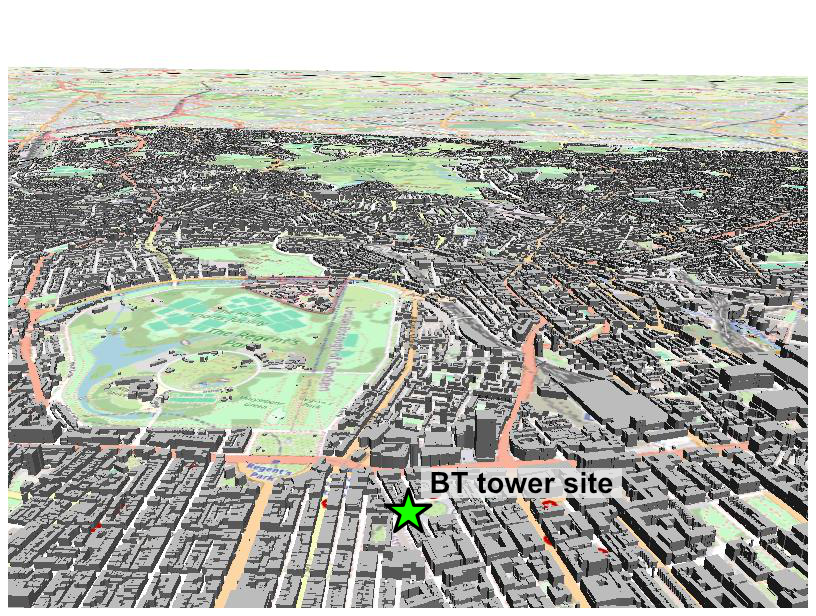
Figure 3Bird's-eye view of buildings located in a region in the Camden borough. These building geometries are part of the static input for the PALM model. Data for the shape and height of buildings are from Ordnance Survey (Ordnance Survey (GB), 2019b, a). Background map is OpenStreetMap (© OpenStreetMap Distributed under the Open Data Commons Open Database License (ODbL) v1.0 (for further information, please see OpenStreetMap)).
3.2 Anthropogenic emission datasets for London
For the London case study, anthropogenic CO2 emissions are derived from the London Atmospheric Emissions Inventory (LAEI) (London Datastore, 2023), published by the Greater London Authority. LAEI employs a bottom-up methodology, combining activity data with sector-specific emission factors to estimate emissions across multiple sectors. The most recent dataset available during this study is LAEI2019, released in 2022, which reports annual total emissions for the year 2019 on a 1 km2 grid covering the region within the M25 motorway. The inventory grid conforms to borough boundaries, so that grid cells intersecting multiple boroughs are subdivided accordingly.
Since LAEI only reports annual total emission on 1 km2 tiles, it is essential to further disaggregate the emission data spatially and temporarily for use in an urban model. A direct approach would be to interpolate the LAEI 1 km2 tile data on the finite difference grid defined in the urban model. However, this approach cannot capture the real emission scenario where emission within a neighbourhood can originated from several large localised emission sources such as gas boilers within households or industrial chimney stacks. While it is ideal to disaggregate all sectors into a fine grid map, there is a lack of available geo-spatial surrogate data for the task. For example, one might be able to find domestic building information in a city to disaggregate domestic energy usage sector, but there rarely exists a comprehensive list of construction site for non-road mobile machinery sector. Therefore, one needs to decide which sectors should be disaggregated with additional surrogate data and which should be simply interpolated. Here, we examine the proportions of each sub-subsector in the LAEI dataset. A list of the sector categories is included in Appendix A. Note that some sub-subsectors have been merged due to their small contribution. For sub-subsectors whose proportions are less than 10 %, their emissions would be simply distributed evenly in the finer grid and in time (annual total amount spread to hourly emission). Otherwise, we consider them to be significant and require fine-scale geospatial data as spatial proxies to disaggregate. In LAEI, CO2 emission is reported for four major sectors (domestic, commercial and industrial, transport, and others) with sub-sectors and sub-subsectors. Figure 4 shows the significant emission sub-subsectors, which are domestic gas combustion, non-domestic (commercial and industrial) gas combustion, road transport, and industrial processes A1 (A1 refers to large industrial point sources).
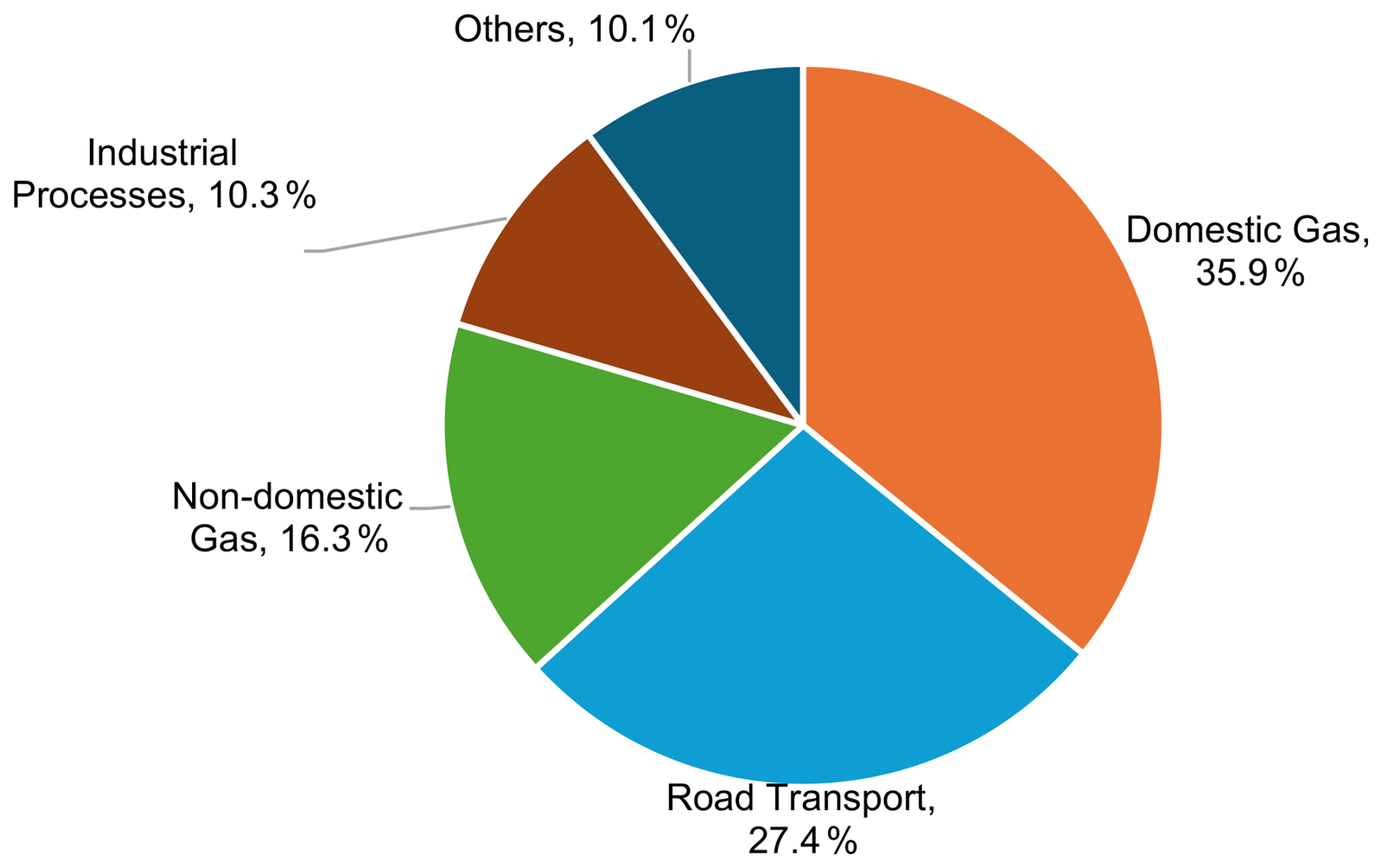
Figure 4Major CO2 emission sub-subsectors in the Greater London Authority region in 2019 – annual emission of sub-subsectors and their proportion in total emissions.
It is noted here that although the word “disaggregation” is used to describe the operation of processing emission inventory data to the desired grid resolution (10 m), data in LAEI for the following sub-subsectors are not used: domestic gas combustion, non-domestic gas combustion, and industrial processes part A1. Instead, the source data for activities that LAEI has used to generate their 1 km2 grid map are retrieved. Together with additional geospatial data as spatial proxies, we processed the 10 by 10 m2 gird map for these sub-subsectors. Road transport was provided in LAEI as shapefile of the major road network and is convenient to interpolate to a grid of 10 by 10 m2.
3.2.1 Spatial disaggregation
Spatial disaggregation of four significant sub-subsectors uses additional geospatial data. These include gas usage within Lower-layer Super Output Areas (LSOAs) or Middle-layer Super Output Areas (MSOAs), industrial point sources inventory, and domestic and non-domestic properties' energy performance certificates (EPC). Each LSOA is a statistical area covering 400 to 1200 households and has 1000 to 3000 residents, while each MSOA contains around 5000–15 000 residents or 2000–6000 households.
For domestic gas combustion, activity data comes from official statistics published by Department for Energy Security and Net Zero in the UK (Department for Energy Security and Net Zero, 2015). The data repository records gas usage (in kWh) in LSOAs. To disaggregate gas usage in LSOAs to households, we obtain property records from Energy Performance of Buildings Data (Department for Levelling Up, Housing & Communities, 2025). Each record in the dataset includes an estimate of annual CO2 emissions for the property which are used as a spatial proxy. This estimation is calculated from many characteristics of a domestic property, for example, the floor area, the floor height, its main heating fuel, and the status of wall and window. We filter domestic properties that use gas as the main fuel, and then utilise their annual CO2 emissions as a spatial proxy to distribute the total gas usage in an LSOA to properties. Then, the sum of gas usage from domestic properties that falls within a title of 10 m by 10 m is taken as the gas usage for the tile. The spatial join operation between the domestic property dataset and the gas usage dataset was performed using the PostgreSQL database with the PostGIS extension. The gas usage in tiles is multiplied by emission coefficient 0.20566 kgCO2 kWh−1 2 to obtain annual emission in the grid map of 10 m by 10 m.
For non-domestic gas combustion, activity data also come from official statistics published by the Department for Energy Security and Net Zero in the UK (Department for Energy Security and Net Zero, 2015). Unlike domestic gas combustion, non-domestic gas usage statistics (measured in kWh) are reported at the MSOA level, which covers a larger geographical area than the LSOAs. To disaggregate gas usage in MSOAs to non-domestic properties, non-domestic energy records from Energy Performance of Buildings Data (Department for Levelling Up, Housing & Communities, 2025) are used, i.e. non-domestic EPC and DEC (display energy certificates). Unlike domestic records, many non-domestic records in this building dataset lack annual CO2 emission estimation. Therefore, another floor_area attribute is used as a spatial proxy. Non-domestic properties that use gas as their main fuel are first filtered, and their floor areas are then used as a surrogate variable to apportion the total gas consumption within each MSOA to individual properties. The gas usage assigned to a 10 by 10 m2 tile is calculated as the sum of the apportioned gas usage of all non-domestic properties intersecting that tile. The gas usage in tiles is multiplied by the emission coefficient 0.20455 kgCO2 kWh−1 3 to obtain annual emission in the 10 by 10 m2 grid-map. It is noted here that the non-domestic heating and power sub-subsector has excluded industrial energy usage in LAEI. Therefore, non-domestic gas combustion only contains those in commercial and industrial properties, i.e. heating and power in such buildings.
For road transport emissions, in addition to the 1 km2 grid-map, LAEI presents a vector dataset of the London major road network stored in a shapefile. Each road section in the shapefile has an attribute for annual transport emission. The shapefile can be rasterised into a 10 by 10 m2 emission grid-map using spatial joint operation. The residual emissions from road transport (which is called minor road transport emission in LAEI) represent about 10 % of the total road transport emission. These emissions are evenly distributed from the 1 km2 grid to the 10 by 10 m2 grid via interpolation.
The industrial processes part A1 in LAEI use data from both the Environment Agency's point source inventory (accessible from https://www.data.gov.uk/dataset/cfd94301-a2f2-48a2-9915-e477ca6d8b7e/pollution-inventory, last access: 15 July 2026) and the National Atmospheric Environmental Inventory (accessible from https://naei.energysecurity.gov.uk/data/maps/emissions-point-sources, last access: 15 July 2026). These inventories include power plants, wastewater processing factories, and other industrial sites. The point sources are spatially joined with the 10 by 10 m2 tiles for a fine emission grid-map.
3.2.2 Temporal disaggregation
The temporal profiles of various sub-subsectors are used to disaggregate annual emissions into hourly emissions. Similarly as in spatial disaggregation, sectors with a proportion less than 1 % are disaggregated using constant temporal profiles. The other sectors use temporal profiles retrieved from CAMS-TEMPO (Guevara et al., 2021) and EDGAR (Crippa et al., 2020). These sectors and their temporal profiles are listed in Table 1.
Table 1Sectors and their temporal profiles. In “Reference” column, CAMS refers to CAMS-TEMPO (Guevara et al., 2021).

Note that a different threshold (1 %) is selected for temporal disaggregation than in spatial disaggregation (10 %). The only additional sub-subsectors (between 1 % and 10 %) are: Industrial Oil/Coal Combustion, Industrial Construction NRMM, and Transport – Aviation. There are temporal profiles for these sub-subsectors in CAMS-TEMPO and EDGAR so we decide to include them in temporal disaggregation as well.
3.3 Vegetation indices and parameter selection
For the London case study, vegetation state variables required by the biogenic CO2 flux model are derived from satellite-based surface reflectance products. Due to frequent cloud cover over the United Kingdom, EVI and LSWI are processed as monthly composites rather than at higher temporal resolution. For each calendar month in 2019, all available cloud-free satellite observations from the corresponding month throughout the 2018–2020 period are selected and temporally mosaicked. The median values are used to generate spatially complete monthly EVI and LSWI fields, reducing data gaps caused by cloud contamination.
The resulting monthly EVI and LSWI maps are provided to PALM as static input variables and are used by the biogenic flux module to represent vegetation phenology and water stress. This approach ensures spatial continuity of vegetation indices while preserving seasonal variability relevant for photosynthesis and respiration.
The parameters of the biogenic model are selected from the VPRM chemistry (WRF-Chem) weather research and forecast model (Skamarock et al., 2019), using parameter sets calibrated against measurements of the flux tower of eddy-covariance in Europe (Lian et al., 2021). Parameters are listed in Appendix F. These parameters are applied uniformly across the study domain, acknowledging that vegetation-specific calibration at the neighbourhood scale is not feasible given the available observations.
3.4 Diagnostic flux averaging configuration
To obtain simulated eddy-covariance (EC) fluxes from the LES, two approaches are employed. The primary approach computes EC fluxes from temporally averaged three-dimensional model fields using Eq. (10). An independent approach uses virtual measurement points that output high-frequency time-series data, from which EC fluxes are calculated following the standard eddy-covariance procedure. The agreement between these two approaches is used to verify the temporal-averaging method.
For the temporal-averaging approach, resolved vertical scalar fluxes are averaged over a 30 min window, consistent with the averaging period used in flux-tower observations. The mean vertical velocity and CO2 concentration are obtained from the standard PALM output, while the covariance term is accumulated online during model integration. These correspond to the , , and terms in Eq. (10). All are 3D output quantities. These fields are then substituted into Eq. (10) in post-processing to obtain a 3D eddy-covariance flux field on all grid points. The 3D EC flux at the exact grid point where the BT tower measurement is located is extracted to compare the simulated EC flux with the site measurement described in the Sect. 3.5.
Besides the EC flux computed via Eq. (10), we also set up virtual measurement points in the domain to show the validity of this temporal averaging method. This is an independent calculation of the EC flux using time-series data. The virtual measurements output velocity component and CO2 concentration at a frequency of 1 Hz, the same as that used in BT measurement (Helfter et al., 2016). After the simulation, 30 min means are computed from the 1 Hz time series and subtracted from instantaneous values to obtain the fluctuations w′ and s′. The EC flux is then calculated as the covariance over each half-hour period. The comparison of the EC fluxes obtained via virtual measurement and via temporal averaging (Eq. 10) is shown in Fig. D1. The two approaches yield almost the same flux profiles. In the main text, we use the EC flux computed from temporal averaging 3D fields as the simulated flux to compare with BT tower measurement.
A 30 min averaging window is used throughout this study to match the averaging period of the BT measurements and standard eddy-covariance processing. While EC fluxes are computed using 30 min averaging intervals, a 2 h moving average is applied to both simulated and measured flux time series when calculating RMSE and correlation coefficients to reduce high-frequency variability. The moving average is computed by taking four half-hourly EC fluxes and compute their mean. The timestamp for the moving average is at the end of the 2 h window.
3.5 BT Tower Eddy-Covariance Measurements and Source Area Characteristics
The measurement site is in Camden, London. An eddy-covariance flux tower was set up on the BT tower in Camden by previous researchers (Wood et al., 2010; Helfter et al., 2011). It collected the vertical CO2 flux (Helfter et al., 2011), turbulent flow quantities (Wood et al., 2010) and other meteorological and greenhouse gas variables. We used the measurements in 2019 to validate our CO2 model. Specifically, the wind speed and the eddy-covariance CO2 flux were used in the validation. The temporal interval of measurements was half an hour. The CO2 flux is computed via the procedure described in Sect. 2.5. In the following, we provide some essential information on the measurement site and its surrounding areas. For more details, the reader is referred to Helfter et al. (2016).
The eddy-covariance (EC) measurements of CO2 were conducted from the BT Tower in central London ( N, W). The EC system was installed on a lattice structure mounted on the roof of the telecommunications tower, providing an effective measurement height of approximately 190 m above street level. The system consisted of a three-dimensional sonic anemometer and a closed-path cavity ring-down spectrometer measuring CO2, CH4 and H2O, with air sampled through a 45 m inlet line. Owing to the unusually large measurement height, the footprint of the observations extended over several kilometres and integrated emissions from a substantial portion of central London.
The BT Tower is located within a densely urbanized area of central London characterized by a mixture of commercial, residential and transport infrastructure. Within a radius of approximately 10 km, the mean building height is 8.8 ± 3.0 m, while typical suburban building heights are 5.6 ± 1.8 m. Consequently, the 190 m measurement height is more than an order of magnitude greater than the average surrounding building height, placing the EC sensors well above the urban roughness sublayer and enabling observation of integrated fluxes from a large urban source area.
Footprint analyses indicate that the source area varies seasonally from a few kilometres under convective conditions to several tens of kilometres during wintertime stable conditions. The footprint encompasses a diverse range of land uses. To the southwest and northwest, the source area includes two major urban parks, Hyde Park (142 ha) and Regent’s Park (197 ha), respectively. Northern sectors are dominated by suburban residential neighbourhoods, whereas eastern and southern sectors contain a mixture of densely built residential and commercial districts. The southeastern footprint also includes part of the River Thames. As a result, the measured CO2 fluxes represent the integrated influence of emissions from road traffic, residential and commercial energy use, and human activities across a heterogeneous urban landscape.
3.6 Evaluation of biogenic module
Because CO2 fluxes measured at the BT tower are dominated by anthropogenic emissions, they provide limited information on the realism of the biogenic component of the model. Therefore, an additional qualitative evaluations of the implemented VPRM scheme were made.
First, we conducted using eddy-covariance measurements from the ICOS site CZ-Lnz, a deciduous forest ecosystem in the Czech Republic (ICOS RI et al., 2023). The objective of this comparison is not to perform a site-specific validation of vegetation fluxes in Regent's Park, but rather to assess whether the model reproduces realistic magnitudes, seasonal variations, and diurnal patterns of net ecosystem exchange (NEE) for deciduous vegetation. Given the climatic and ecological differences between the two sites, the comparison is interpreted as an assessment of the VPRM implementation rather than as a direct validation of local biogenic fluxes.
The CZ-Lnz site is located in a deciduous floodplain forest, and its eddy-covariance measurements are primarily influenced by local biogenic carbon exchange. Although the climatic and ecological conditions differ from those in London, CZ-Lnz provides a long-term, high-quality record of net ecosystem exchange (NEE) from a deciduous forest ecosystem, allowing a qualitative assessment of the VPRM representation of forest carbon uptake and respiration.
Monthly ensemble averages of tower observations were used to derive representative half-hourly diurnal NEE profiles for each month. For the model, NEE was extracted directly from the VPRM output for a grid cell in Regent's Park classified as deciduous forest. The comparison therefore focuses on the temporal characteristics of NEE rather than on direct site-to-site agreement.
Second, the total NEE for the parent domain (roughly Greater London Authority area) was compared with the ICOS-VPRM product (Gerbig and Koch, 2021). This product runs offline VPRM module with MODIS-derived satelite indices and meteorological inputs from ECMWF IFS analysis data. The product has a spatial resolution of ∼ 0.1°. The daily sum of NEE for the twelve simulated days from PALM-CO2 and from ICOS-VPRM were compared. Using the simulated days as representative values for their corresponding months, annual NEE rate (both total amount and monthly correlation) were reported.
3.7 Modelling settings in PALM-CO2
3.7.1 Static driver
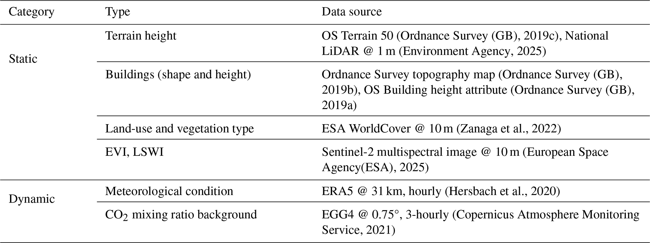
As an urban model, PALM takes all the data describing urban land surface within one file called the static driver. These data include terrain height, land-use type and building geometries. The data sources for static inputs in the study area are listed in Table 2. The static input file is prepared with an open source tool GEO4PALM (Lin et al., 2024).
For buildings' geometry, the topography map from Ordnance Survey (OS) (Ordnance Survey (GB), 2019b) is used. The full topography map is filtered to include buildings only. For buildings' height, an additional OS building height dataset (Ordnance Survey (GB), 2019a) is used. The shapes (geometries) and the heights of buildings are matched with unique IDs indexed by OS to form a vectorised building map. For terrain height, two data sources of different resolution are selected for the parent and child domain, namely OS Terrain 50 (Ordnance Survey (GB), 2019c) (resolution at 50 m) and National Lidar Programme (Environment Agency, 2025) (resolution at 1 m). Land-use and vegetation types are retrieved from ESA WorldCover dataset (Zanaga et al., 2022).
Using these static input data, we activated the following surface modules. An urban surface module solves for the buildings' energy balance and energy exchange with outdoor environments. A land surface module computes the drag and heat dispersion in different land-use types, including vegetation, pavement, water, and soil. Land-use types also affect radiation from and into the urban surface. The soil temperature is modelled with an eight-layer energy balance equation.
3.7.2 Initial and boundary conditions (dynamic driver)
The initial and boundary conditions are taken from real meteorological data from the ECMWF reanalysis dataset (ERA5) (Hersbach et al., 2020). These are prepared as a “dynamic driver” file in PALM. ERA5 model level data for hourly velocity, potential temperature, humidity, long- and short-wave radiation, and surface level pressure are used to drive the urban model simulation.
For CO2 transport, the background value of its mixing ratio is also required on the boundary outside the modelling region. This information comes from CAMS global greenhouse gas reanalysis (EGG4) (Copernicus Atmosphere Monitoring Service, 2021), due to its spatially and temporally consistent global coverage and suitability for boundary forcing in regional atmospheric transport simulations. 3-hourly CO2 mixing ratio in the study region is used as the background value on the boundary. It is interpolated into hourly data and written in the dynamic file. These dynamic driven data sources are also listed in Table 2.
(Ordnance Survey (GB), 2019c)(Environment Agency, 2025)(Ordnance Survey (GB), 2019b)(Ordnance Survey (GB), 2019a)(Zanaga et al., 2022)(European Space Agency(ESA), 2025)(Hersbach et al., 2020)(Copernicus Atmosphere Monitoring Service, 2021)Table 2Data sources for static and dynamic drivers in the study area.
3.7.3 Running on HPC
The case is set up to running on ARCHER2 (UK HPC) using 1274 cores, out of which 250 cores are used for the parent domain (N01) with 10 by 25 subdomains in the x and y directions and the rest 1024 cores are used for the child domain (N02) with 32 by 32 subdomains in the x and y directions. The 16th day of each month in 2019 is selected for the simulation at the study area. Depending on the average wind speed of the day, the CPU wall time for one day simulation takes between 6.1 h (for 16 April) and 23.2 h (for 16 March).
4.1 Validation against BT tower measurement
In this subsection, we show comparison of the modelled flux and the measured flux by the eddy covariance method. This comparison validates: (1) the input anthropogenic emissions and online-computed biogenic fluxes, and (2) the CO2 transport process calculated by PALM.
In previous studies, CO2 transport has been approximated using simplified two-dimensional advection–dispersion approaches, in which turbulent source areas or flux footprints were parameterized rather than explicitly resolved; see Christen et al. (2011) for an urban carbon emission model that leverages the 2D model for validation. In contrast, PALM resolves 3D turbulence using large-eddy simulation, enabling a more detailed representation of turbulent dispersion and vertical transportation processes, and thereby providing a more physically consistent characterization of source-receptor relationships.
To reduce the influence of high-frequency variability and facilitate comparison between simulated and measured fluxes, both time series were additionally smoothed using a 2 h moving average prior to the calculation of RMSE and correlation coefficients. The 30 min EC fluxes were retained for all other qualitative analyses. Wind speed and wind direction have also been smoothed using the same method.
Figure 5 shows the validation results for the CO2 flux for selected months representing each season of a year. Overall, good agreement between the simulated CO2 flux and the measurement at the BT tower has been reached. When July is excluded, the average RMSE and correlation coefficient are 16.74 µmol m−2 s−1 and 0.74, respectively. The trend of the diurnal cycle has been captured by the model and matches well with observations. Specifically, the CO2 flux remains low in the early morning before sunrise, increases during the morning hours (08:00 a.m. to 12:00 p.m.), reaches a peak in the afternoon (04:00 p.m. to 06:00 p.m.), and gradually decreases toward midnight (00:00 a.m.). As the measurement site is located in a commercial-residential mixed area with limited green spaces, the flux pattern is dominated by anthropogenic emission. Therefore, such a diurnal cycle meets the expectation of human activity patterns within a day. Quantitatively, the magnitudes of fluxes in January, April, and October show good agreement with observations. Statistics show relatively low error and high correlation between simulation and measurement.
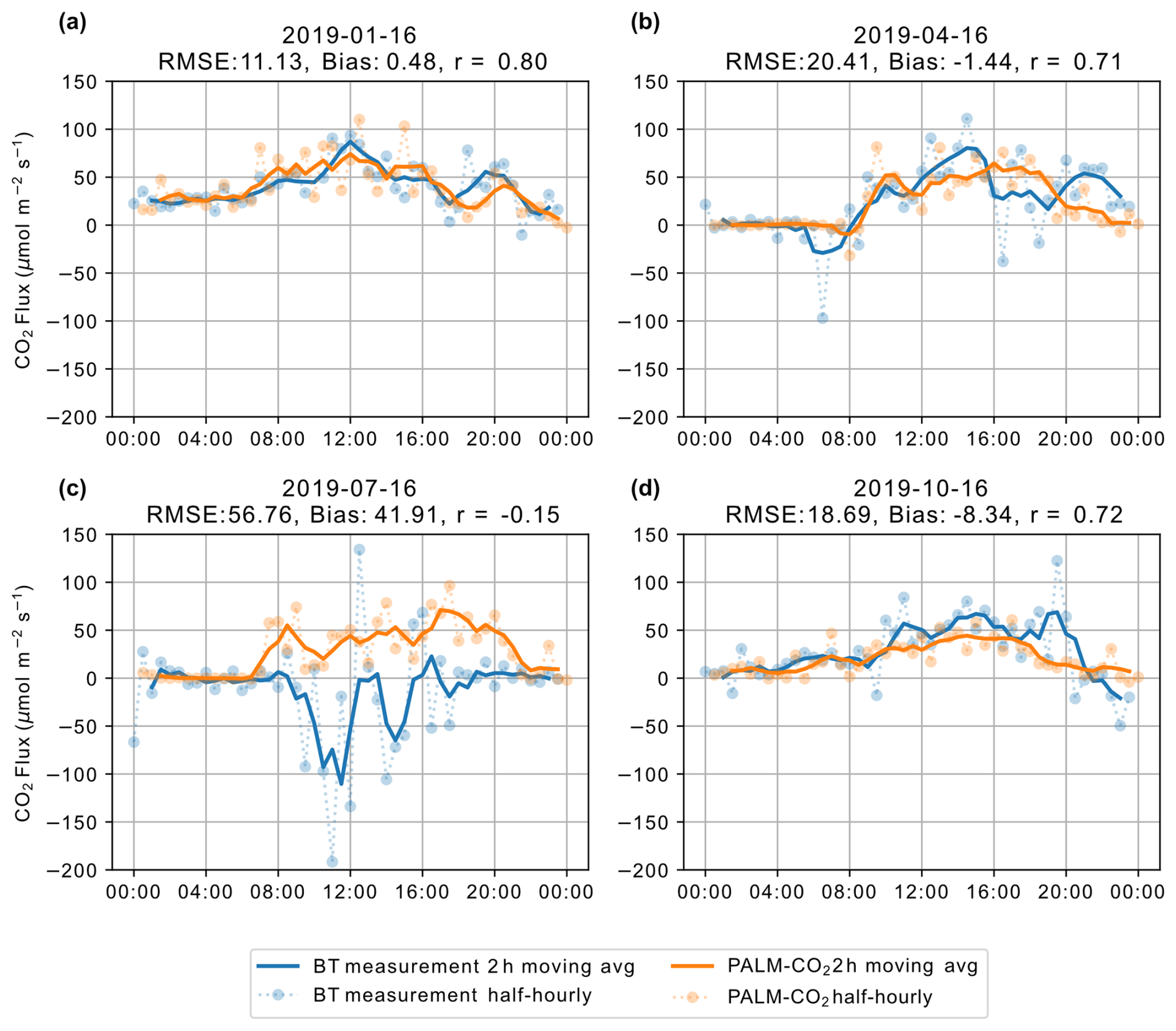
Figure 5Comparison of modelled CO2 fluxes and BT tower measurements in 2019. Dotted lines and markers show original temporal data at half-hourly resolution for both PALM model and tower measurements. Solid lines show two-hour moving average. All times in the figure are in local time. Sporadic missing data in measurement have been filled with interpolated values. (a) 16 January 2019; (b) 16 April 2019; (c) 16 July 2019; (d) 16 October 2019.
Modelled fluxes in July show a consistent pattern as in other seasons, while discrepancy from measurement exists. The site measurement in 16 July has poor quality which already shows a non-typical diurnal pattern in the figure. Besides, an overestimation of flux on 16 July persists. As one would expect that anthropogenic emission in July (summer time) is smaller than in October and January, yet the simulated flux in July is higher. This overestimation originates from extremely weakly forced atmosphere during daytime peak hours. As can be seen in Fig. 6c, wind speed at 190 m height is close to 1 m s−1 between 10:00 to 16:00. Poor advection caused build-up of CO2 in the domain and an over-estimation of EC flux. The quality control flag and additional analysis of July data can be found in Appendix C.
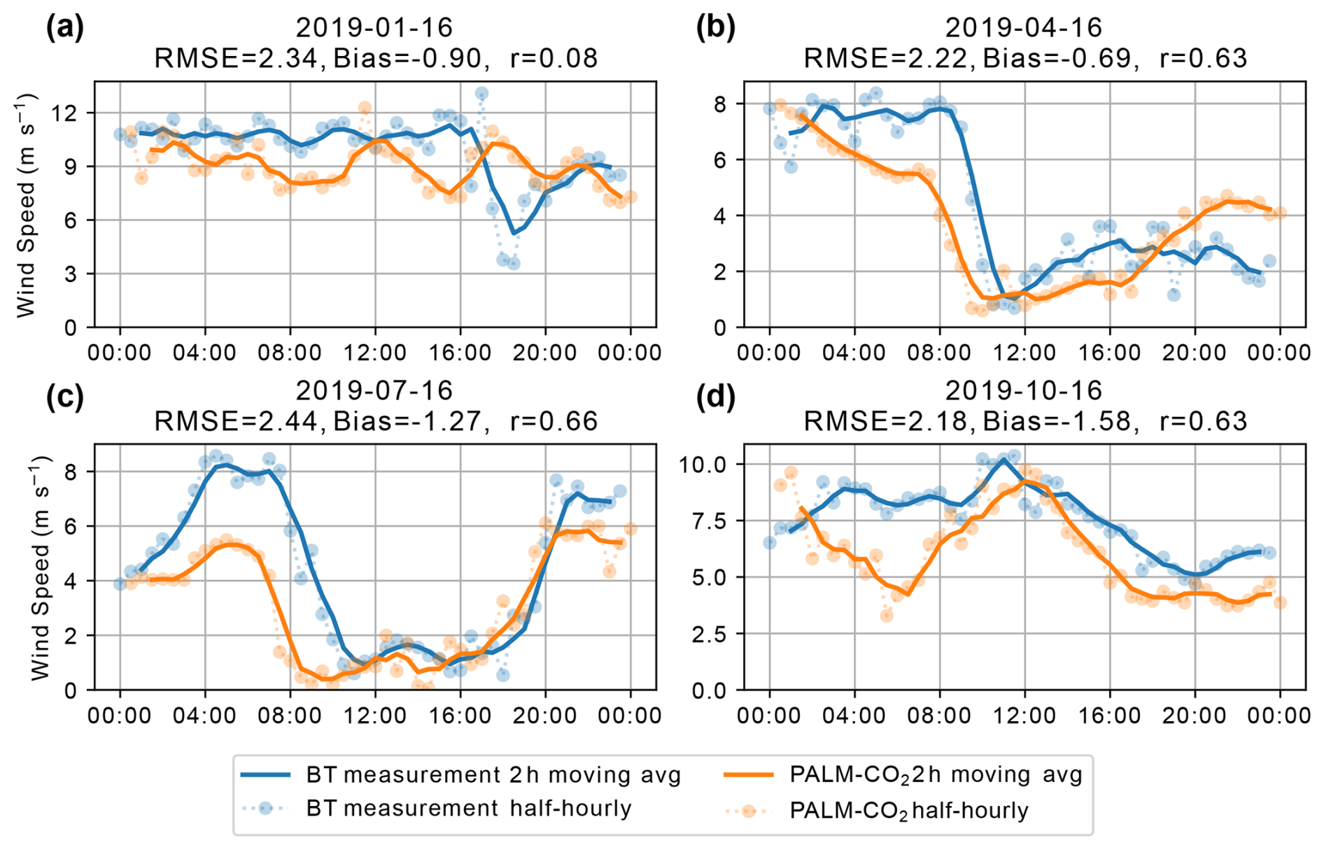
Figure 6Comparison of modelled wind speed and BT tower measurements in 2019. Dotted lines and markers show half-hourly averaged wind speed from simulation and measurement. Solid lines show two-hour moving average. Sporadic missing data in measurement have been filled with interpolated values. (a) 16 January 2019; (b) 16 April 2019; (c) 16 July 2019; (d) 16 October 2019.
Figures 6 and 7 show validation of the wind speed and direction. The average RMSEs for wind speed and wind direction in the figures were 2.30 m s−1 and 37.50°, respectively, while the corresponding average correlation coefficients were 0.50 and 0.68. The wind velocity on the 10 by 10 m2 grid at 190 m height corresponding to the measurement location is extracted from the simulation. In the figures, wind speed and direction at a half-hourly interval and its 2 h moving average daily profile are shown. The general trend of daily variation of wind (the 2 h moving average profile) matches that in the measurement. For all days simulated in 2019, statistics show good agreement between simulation and measurement for both wind speed and direction, with average RSME around 2.4 m s−1 and 28.65° and correlation coefficient 0.55 and 0.75 (see Appendix B). The validation results demonstrate that ERA5 provides suitable dynamic boundary conditions for the parent domain and confirm the effectiveness of the nesting strategy in representing processes within the nested domain.
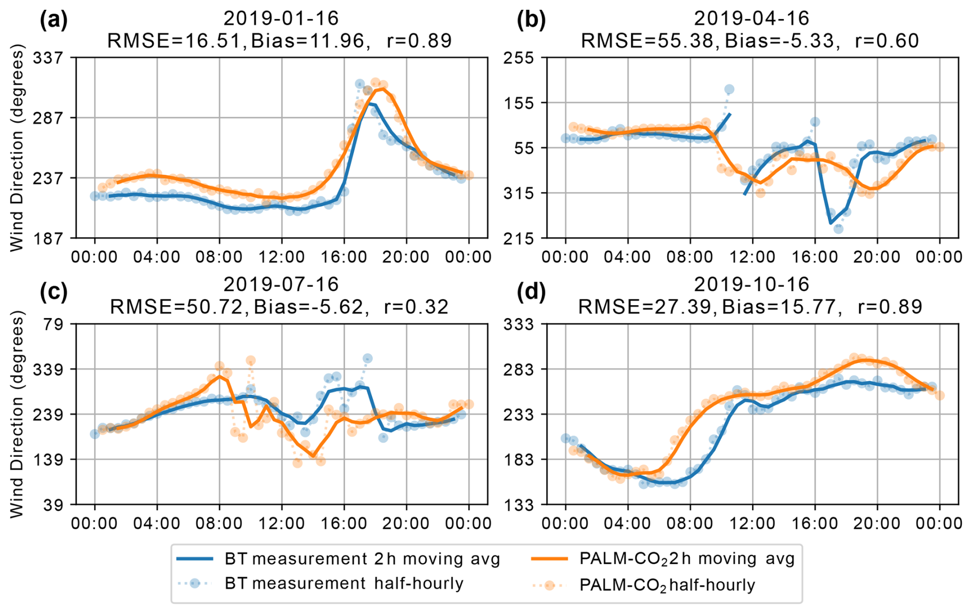
Figure 7Comparison of modelled wind direction and BT tower measurements in 2019. Dotted lines and markers show half-hourly averaged wind speed from simulation and measurement. Solid lines show two-hour moving average. Sporadic missing data in measurement have been filled with interpolated values. (a) 16 January 2019; (b) 16 April 2019; (c) 16 July 2019; (d) 16 October 2019.
Results for all months can be found in Appendix B.
4.2 Evaluation of biogenic fluxes
Comparison with the BT tower measurements provides the primary validation of the modelling framework in the study area. However, CO2 fluxes measured at the BT tower are dominated by anthropogenic emissions, making it difficult to directly assess the realism of the vegetation component of the model. Here, we compare biogenic flux with two independent sources in the literature to evaluate the biogenic fluxes in PALM-CO2.
To provide an independent evaluation of the implemented VPRM scheme, we first compare the simulated biogenic fluxes against eddy-covariance observations from a European forest site, Lanzhot in Czech (CZ-Lnz) (ICOS RI et al., 2023). The purpose of this comparison is not to perform a site-specific validation of vegetation in Regent's Park, but rather to assess whether the model produces realistic magnitudes, seasonal variations, and diurnal cycles of ecosystem carbon exchange.
Figure 8 compares the simulated and observed NEE profile. Both datasets exhibit the expected seasonal behaviour of temperate deciduous forests. During winter (December, January, February), NEE remains relatively small and positive, reflecting limited photosynthetic activity and continued ecosystem respiration. During summer (May, June, July), stronger daytime carbon uptake produces larger negative NEE values and a pronounced diurnal cycle. The model reproduces these broad seasonal and diurnal characteristics, indicating that the implemented VPRM module captures the dominant controls on biogenic carbon exchange.
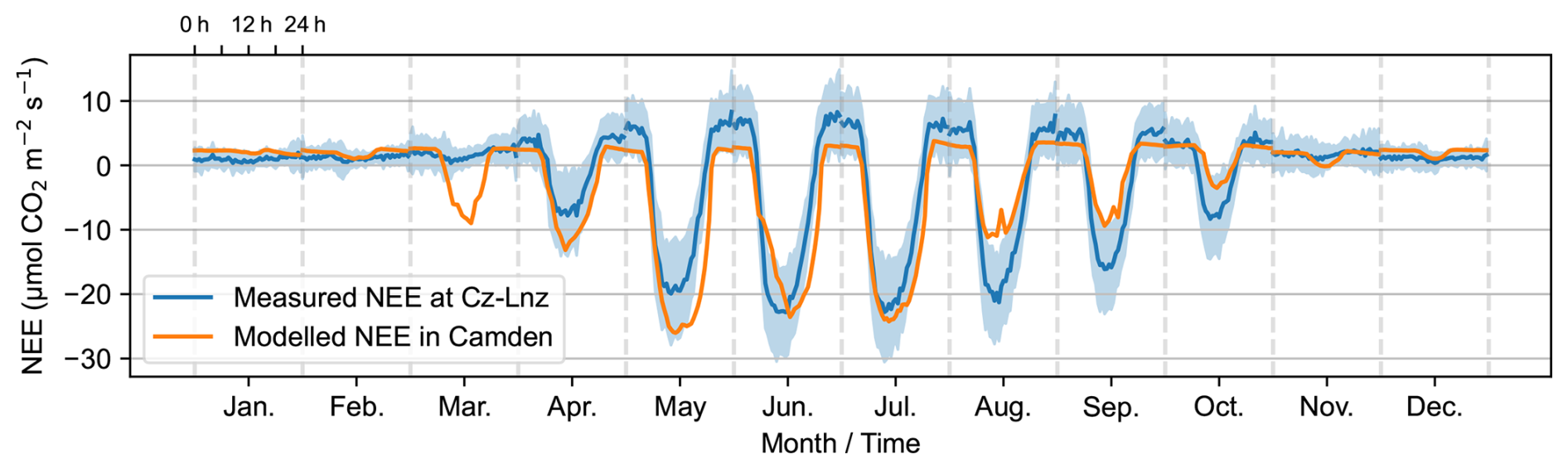
Figure 8Comparison of monthly 24 h net ecosystem exchange profile from flux tower measurement and from PALM model. The vegetation type is deciduous trees. The measurement location is at Lanžhot in Czech Republic (CZ-Lnz). Shaded area is the standard deviation range for measurement. Vertical dashed lines denote month boundaries.
Differences are evident during the spring green-up period and autumn senescence. The simulated NEE shows stronger carbon uptake in March and April and weaker uptake in August, September and October compared with CZ-Lnz observations. These discrepancies are likely related to differences in phenology between the two sites since they correspond to the budburst and senescence stages of deciduous forests (Duchemin et al., 1999). The timing of budburst and senescence is influenced by local climate, species composition, soil conditions, and management practices, all of which differ between the urban park environment of Regent's Park and the rural floodplain forest represented by CZ-Lnz. As shown in Fig. 9, EVI and LSWI increase rapidly in March at the Regent's Park location, leading to enhanced simulated GPP through Eq. (2).
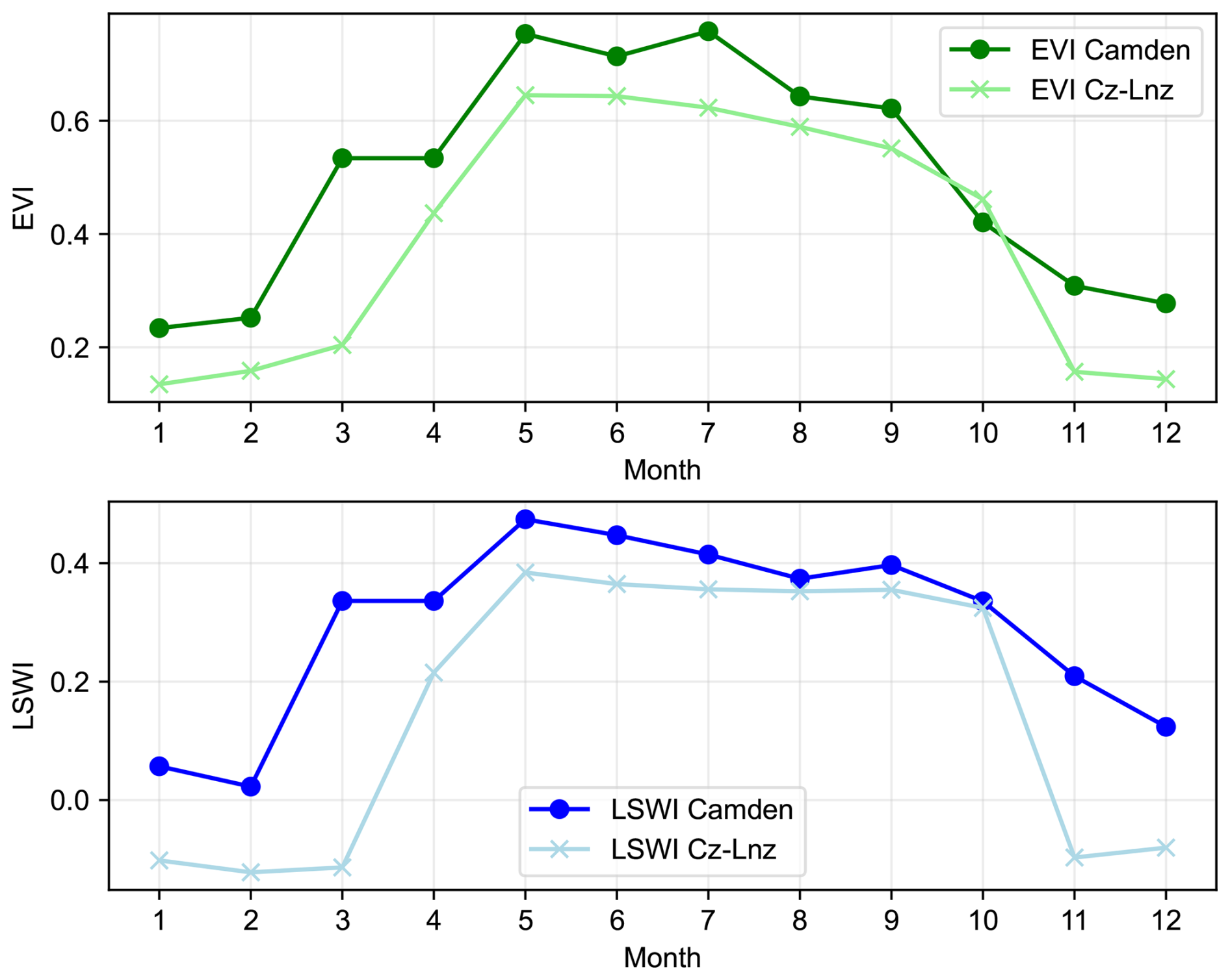
Figure 9Comparison of monthly EVI and LSWI at two deciduous forests site: Regent Park in Camden, and Lanžhot in Czech Republic (CZ-Lnz). Biogenic fluxes in both sites are compred in Figure 8.
The stronger uptake simulated during spring is consistent with the rapid increase in EVI and LSWI at the Regent's Park location. However, the differences observed during late summer and early autumn cannot be explained by EVI alone. Although EVI remains relatively high during August and September, NEE is influenced by additional environmental controls in VPRM, including temperature and moisture stress, as well as site-specific ecosystem characteristics. Furthermore, the comparison involves two ecologically distinct systems: an urban park in London and a rural floodplain forest in the Czech Republic. Differences in species composition, soil moisture conditions, forest structure, and phenological timing may therefore lead to different seasonal trajectories of carbon uptake despite similar vegetation index values. Consequently, the late-summer discrepancy is likely attributable to site-specific ecological differences rather than changes in canopy greenness alone.
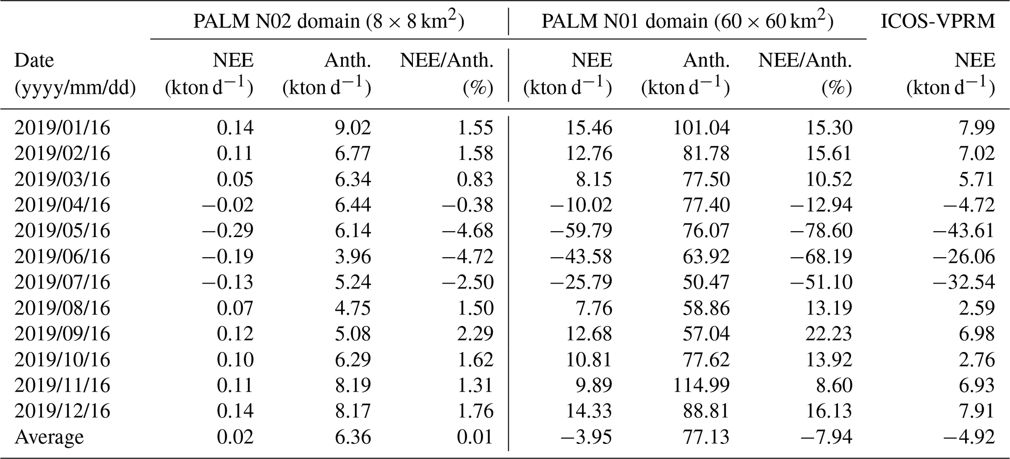
Second, the sum of the total biogenic flux in the N01 domain (60 by 60 km2) is compared with the ICOS-VPRM product (Gerbig and Koch, 2021). Figure 10 shows the comparison. The annual trend of biogenic flux computed in PALM agrees with that in ICOS-VPRM in general. A positive net flux during winter, late summer and autumn seasons appeared in both computations, while spring and early summer show negative net flux. The values are listed in Table 3. Using the NEE on the 16th day of each month to represent monthly flux, average biogenic flux in 2019 is −3.95 kton d−1 in our model while ICOS-VPRM reports average NEE −4.92 kton d−1. Correlation coefficient between them is 0.97. To show the ratio of biogenic fluxes and anthropogenic emissions, Table 3 also lists the total biogenic fluxes in the N02 domain (8 by 8 km2) as well as the N01 domain. For the N02 domain, biogenic flux to anthropogenic flux ratio is between −4.72 % to 2.29 %; for the N01 domain the ratio is between −78.2 % and 8.6 %. This shows that in the densely populated Camden borough biogenic fluxes have very limited offset to anthropogenic emissions.
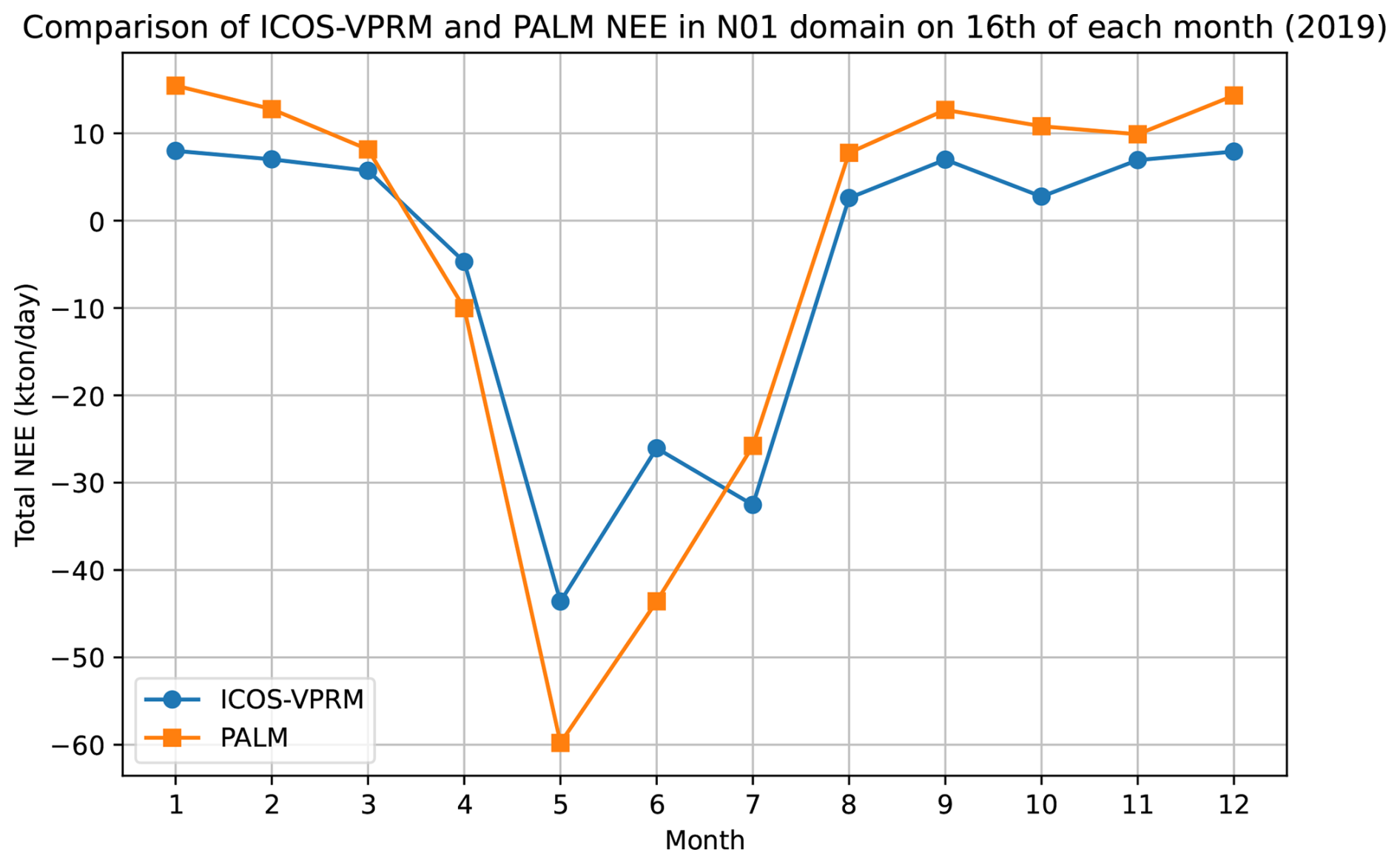
Figure 10Comparison of daily total biogenic flux (NEE) computed by PALM and in the ICOS-VPRM product. Total fluxes in the N01 domain (60 by 60 km2) is plotted. For ICOS-VPRM, the area is approximated as the grid does not align exactly with the BNG projection used in PALM.
Table 3Daily integrated NEE and anthropogenic CO2 emissions on the 16th day of each month in 2019. NEE values are reported for the PALM N02 domain (8 × 8 km2), the PALM N01 domain (60 × 60 km2), and the ICOS-VPRM product over approximately the N01 domain.
4.3 Urban boundary flow and carbon dioxide concentration
In this subsection, we show results on carbon dioxide concentration and its relation to the height of the Atmospheric Boundary Layer (ABL). Three snapshots of CO2 concentration in the morning 08:30 a.m., noon 12:30 a.m., and evening 08:30 p.m. are selected in the following analysis. The ABL heights and Obukhov lengths for the snapshots are listed in Table 4. Figure 11 shows the CO2 concentration at the surface level at selected times during a day in January and July. Due to terrain height and building geometries, the surface level at different horizontal places are at different levels. This has been processed and in the figure only the lowest level in the air is plotted. In all three snapshots in both January and July, individual large anthropogenic emission locations such as major roads and buildings in the commercial region (lower right in each sub-figures) can be identified. They contribute substantially to the variation of local concentrations. In January, due to a relatively higher wind speed (about 10 m s−1, see Fig. 6a), advection near the ground level is prominent throughout the day. However, its effect weakens around noon (12:30 p.m.), due to an increase in upward turbulent flow driven by ground heating in the air. At night, reduced heat turbulence causes a build-up of CO2 in the region. In July, the wind speed is lower (about 4 m s−1, see Fig. 6c). In the morning, only limited advection occurs due to weak lateral wind and minimal heat turbulence. Therefore, a large concentration region appears in the dense commercial region (lower right in the sub-figure). At noon, due to increased heat turbulence and upward flow, concentration is reduced in the region. At night, mixed effects from suppressed upward turbulence and increased lateral advection (due to increased wind speed) produce a moderate concentration. 24 h surface concentration profiles for the two days discussed here can be found in Appendix G.
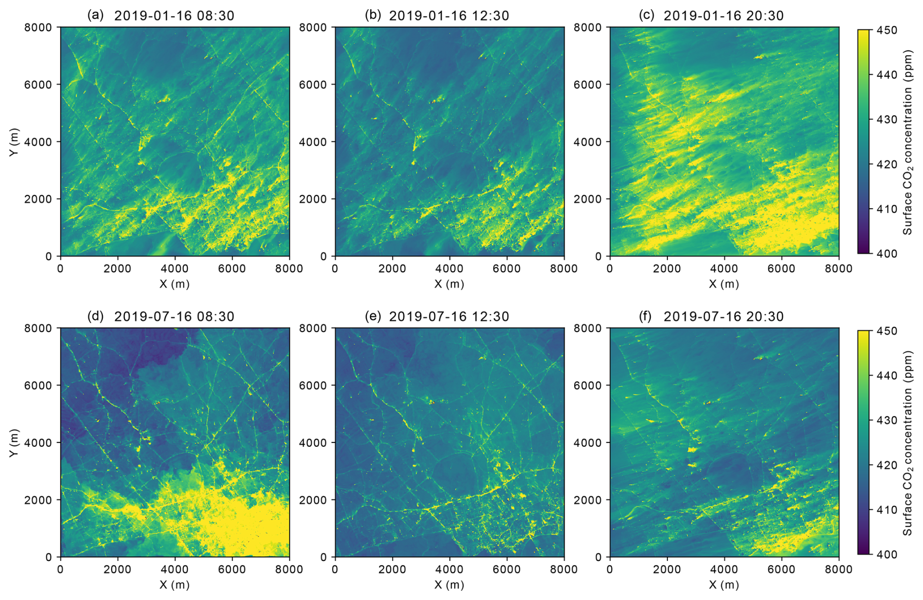
Figure 11Instantaneous surface level CO2 concentration at different times in January (a–c) and July (d–f) from the LES simulation.
Table 4ABL height statistics and Obukhov length for 16 January 2019 and 16 July 2019.
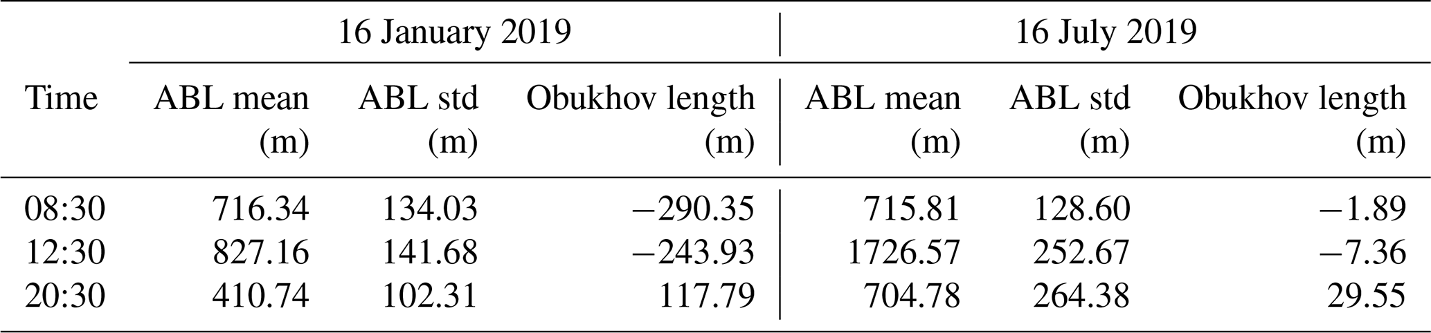
The January cases are characterized by a relatively shallow boundary layer (411–827 m) and near-neutral to weakly unstable/stable conditions ( 100–300 m). In contrast, the July cases exhibit substantially stronger instability during daytime (L=−1.9 to −7.4 m), leading to enhanced turbulent mixing and the development of a deep convective boundary layer reaching 1.7 km at midday. Following sunset, both periods transition to stable stratification (L>0), accompanied by a reduction in boundary-layer height, although the summer boundary layer remains considerably deeper than the winter boundary layer due to stronger daytime heating and residual turbulence. The ABL height and stability are reflected in the vertical CO2 concentration profile. Figure 12 shows the concentration on a x=4000 m vertical cross-section over the domain at different times in January and July. The location of the vertical cross-section is shown in Fig. 2b. In general, during morning and night, the shallow boundary layer traps CO2 below approximately ABL height, while during the day the ABL is thicker and the unstable ABL can mix CO2 well. An exception occurs in the morning (08:30 a.m.) in January when advective transport lifts some plumes above the boundary layer, reducing near-surface accumulation.
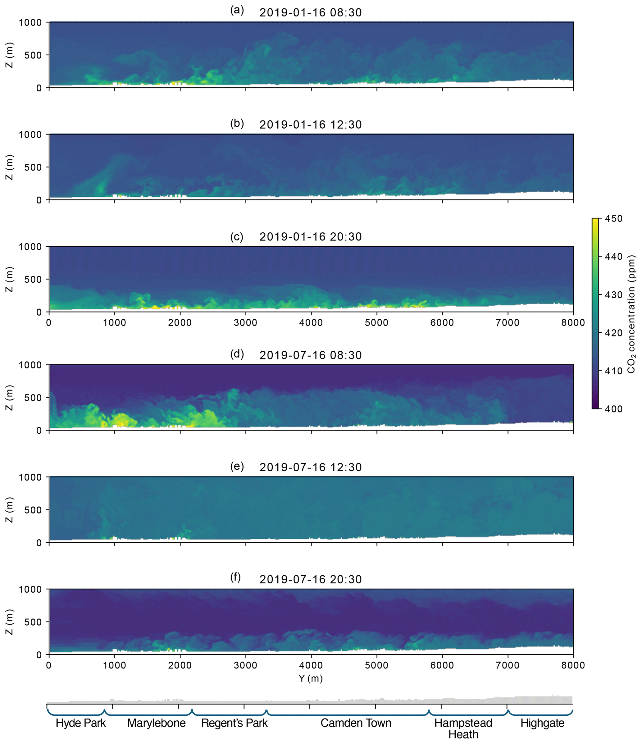
Figure 12Instantaneous CO2 concentration at x=4000 m cross-section in the domain at different times in January (a–c) and July (d–f). LES results are shown here. On the bottom the annotated axis illustrates the topography and geographic references along the cross-section. For ABL heights and stability corresponding to the snapshots see Table 4. The location of the vertical cross-section is shown in Fig. 2b.
Figure 12 also shows the impact of spatial patterns of anthropogenic emissions on CO2 concentrations within the lower atmospheric layer. As shown in the geography tags, urban land-use types are interwoven from south to north (+Y direction in the figure), alternating commercial districts and green spaces: beginning with parkland (Hyde Park), followed by dense commercial areas (Marylebone), then another parkland and commercial areas (Regent's Park and Camden Town), mixed natural land and residential zones (Hampstead Heath and Highgate). Concentration hotspots correspond to densely populated areas with higher human activities. Throughout the day and in both months, the effect of turbulent dispersion (plumes) can be clearly observed in the figure.
The above pattern is revealed through LES that explicitly represents urban topography and spatially heterogeneous anthropogenic and biogenic fluxes at a 10 m resolution. The resulting complex CO2 dispersion pattern highlights the importance of resolving urban-scale flow structures and emission heterogeneity when simulating urban carbon transport. On this basis, the model can help constrain emission patterns in an inversion problem. This conclusion echoes the argument in Brunner et al. (2019) that vertical distribution of carbon fluxes greatly affects the transport process.
4.4 Grid sensitivity study
The grid resolution in the case study was selected as 10 m in the child domain. This is a balance between resolution, availability of static and dynamic driver data, and the purpose of the carbon dioxide case study in general. From the perspective of numerical discretisation, one wishes to have a high resolution to resolve turbulent transport at as small scales as possible. However, this can be prohibitive for computational cost. It also suggests a new requirement for static and dynamic drivers. For static driver, it requires finer topography data (buildings and terrain height), land use data, and vegetation data which could be scarce. Yet from the perspective of the user end, a study on carbon dioxide does not require as fine a resolution as those used in air pollution study where the individual exposure can benefit from a finer concentration map. Eventually, we selected the 10 m resolution in the main case study.
Nevertheless, it is worth exploring the turbulent transport process at different grid resolution. Here, we include two additional simulations of an ideal convective boundary layer (CBL) case at 10 and 5 m resolution and compare the results. The domain is 2 km by 2 km by 3.5 km, i.e. a smaller area surrounding the BT tower in the child domain in the main case study shown in Fig. 2. The 2 km domain is created using the same Ordnance Survey data for terrain height and buildings at 10 and 5 m resolution while the flow and emission conditions are controlled. The flow is driven by both the geostrophic wind, ug=5 m s−1 and vg=5 m s−1 and the bottom heating at 0.1 K m s−1. These values are typical in the study area. The side boundaries for momentum and temperature are cyclic. The top boundary for momentum is the free slip, while for energy it is a constant gradient at 0.01 K m−1. The emission of passive scalar CO2 is set as a constant rate in time but spatially heterogeneous, whose pattern is determined by a typical winter day in the study area. The side boundaries for CO2 are set as 0, while the top boundary is zero gradient Neumann. The initial flow field is geostrophic wind. The initial potential temperature is constant below 800 m and increasing at 0.01 K m−1 until the top boundary to form an inversion layer. The initial concentration for CO2 is set as 0. Both cases have been run for 48 h. Horizontally, the grid resolution is 10 and 5 m respectively. Vertically, below 400 m the grid resolution is 10 and 5 m respectively, while above 400 m the grid space increases at a ratio of 1.08 until reaches approximately 3.5 km.
Figure 13 shows the vertical flux profile at the end of simulation (48 h) for two grid sizes. Note that the temporal mean is used to compute the turbulent fluctuation and turbulent flux for subplot (a) and (e), while spatial (horizontal) mean is used for the purpose in the rest subplots. In Fig. 13b and f, resolved fluctuations are defined using horizontal averaging. As a result, the resolved flux may include contributions from persistent spatial heterogeneity arising from terrain-induced flow structures and spatially varying emission patterns. Therefore, the resolved flux fraction should be interpreted as the portion of transport resolved by the LES grid, rather than as a strict decomposition between turbulent and dispersive transport processes. This interpretation becomes more reliable above the roughness sublayer, where turbulence is increasingly horizontally homogeneous and the influence of dispersive motions associated with surface heterogeneity is diminished. In the current case, average building height or roughness height is about 37.7 m for 10 m grid resolution and 33.2 m for 5 m grid resolution.
Overall, the flux profiles obtained with the two grid resolutions show good agreement at intermediate and higher elevations, particularly above approximately 75 m (about two roughness heights). Below this level, however, notable differences emerge. As shown in Fig. 13a and e, the turbulent flux at 5 m resolution exhibits a larger standard deviation, reflecting the stronger influence of surface heterogeneity captured by the finer representation of urban morphology, including street canyons, building geometry, and spatially varying emission patterns.
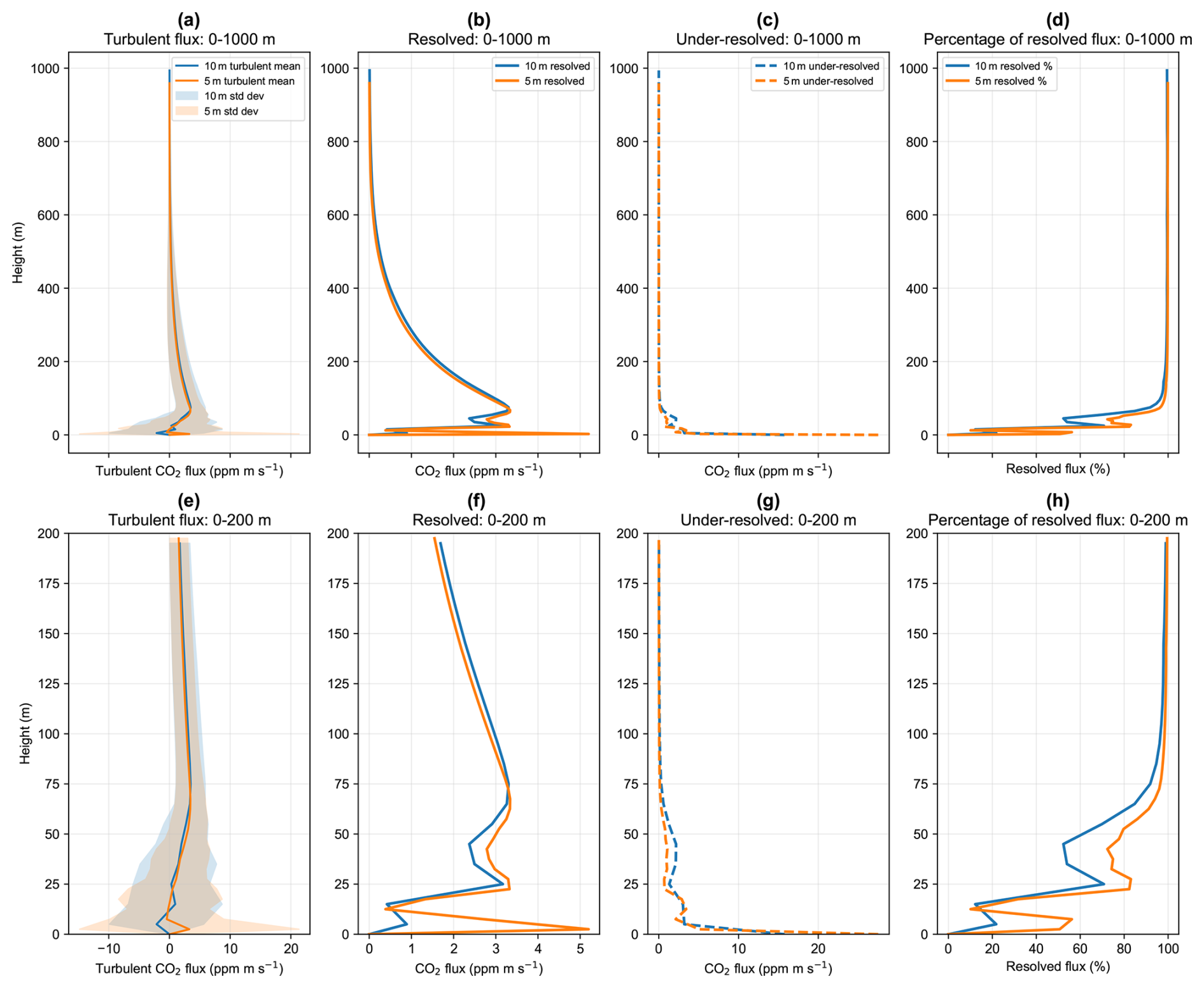
Figure 13Comparison of vertical turbulent flux profile at 48 h of the 10 and 5 m resolution simulations. (a) The horizontal mean (solid line) and standard deviation range (shaded area) of turbulent flux computed from temporal average Eq. (12) on each vertical level; (b) resolved turbulent flux computed from spatial average; (c) under-resolved turbulent flux computed from spatial average; (d) percentage of resolved flux. (e)–(f): zoomed-in view of (a)–(d) for 0 to 200 m height.
The extent to which turbulent transport is resolved also differs within the roughness sublayer, as illustrated by the profiles of resolved and under-resolved turbulent fluxes in panels b–d and f–g. Below 75 m, the 5 m simulation resolves a greater fraction of the turbulent flux than the 10 m simulation. At higher elevations (> 100 m, or roughly three roughness heights), both resolutions resolve the vast majority of the turbulent transport, with resolved flux fractions exceeding 96.9 % and 98.5 % for the 10 and 5 m simulations, respectively. At 190 m, corresponding to the height of the BT Tower measurements, the resolved flux fractions are 98.9 % for both grid resolutions.
These results indicate that, under convective boundary-layer conditions, a 5 m grid resolution provides a more accurate representation of surface heterogeneity and turbulent transport within the lower urban canopy and roughness sublayer (up to approximately three roughness heights). Above this region, however, turbulent transport of passive scalars is already well resolved at a 10 m grid resolution. Additional details of the grid-sensitivity experiment and model configuration are provided in the Appendix D.
4.5 Ensemble simulation of a representative validation case
While the validation in previous subsections show promising agreement, it should be noted that the LES presented there represents only one realisation of turbulent flow field for a given day. Because atmospheric turbulence is chaotic, even under identical large-scale forcing and boundary conditions, small perturbations in the turbulent field can lead to different instantaneous evolutions. Therefore, a perfect match between a single LES realization and the measured half-hourly eddy-covariance fluxes should not be expected. To better quantify the variability associated with turbulent realization uncertainty, a 10-member ensemble simulation was performed for 16 October 2019.
The ensemble members were generated by using different random number seeds in the PALM synthetic turbulence generator, while keeping all other model settings unchanged. In this way, the ensemble isolates the sensitivity of the simulated EC flux to differences in the turbulent realization, rather than to changes in forcing, domain configuration, or model physics.
Figure 14 shows the half-hourly EC flux from all 10 ensemble members together with the ensemble mean. At the native 30 min resolution, both the model output and the measurements exhibit strong short-term fluctuations. Such variability is expected for turbulent fluxes and makes a direct point-by-point comparison between simulation and observation difficult, especially when the purpose is to assess whether the LES reproduces the overall temporal evolution and magnitude of the fluxes. For this reason, the comparison was additionally carried out using a 2 h moving average, applied consistently to both the LES output and the measurements. This smoothing reduces the influence of high-frequency fluctuations while retaining the diurnal structure of the flux evolution.
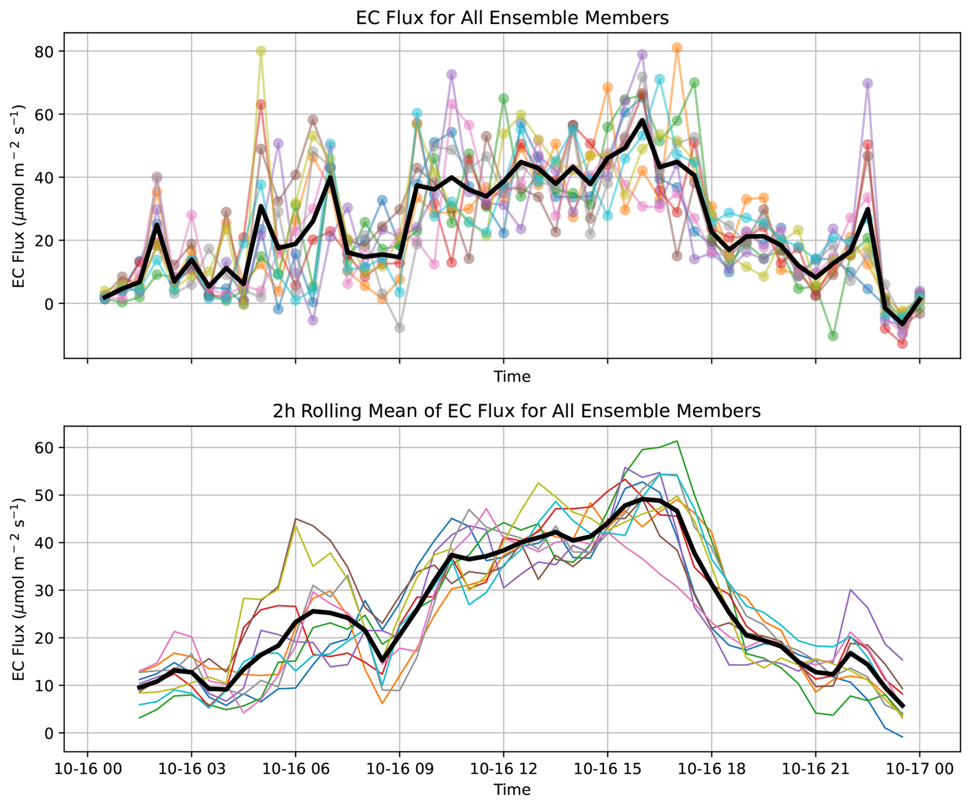
Figure 14Ensemble members for 16 October 2019 and their mean. Top plot shows original half-hourly EC flux processed from LES; bottom plot shows 2 h moving averaged EC flux. Thin coloured lines represent individual ensemble members. Thick black lines represent their means.
The smoothed ensemble results indicate that, despite substantial spread among individual members at half-hourly resolution, the realizations show a broadly consistent diurnal pattern after applying the 2 h moving average. The ensemble mean captures the main daytime increase in EC flux, with values rising from low nighttime and early-morning levels to a midday/afternoon maximum, followed by a decline toward evening. This suggests that the large-scale temporal development of the flux is robust across different turbulent realisations, whereas part of the short-term mismatch between a single simulation and the observations can be attributed to intrinsic flow variability.
Figure 15 compares the measured EC flux and the ensemble mean using the 2 h moving average. The black line represents the ensemble mean, and the shaded band indicates the uncertainty range of the ensemble mean given by the standard deviation. The red line shows the smoothed measurements. Overall, the ensemble mean reproduces the broad diurnal evolution seen in the observations, including the increase during the morning, elevated daytime fluxes, and the decrease in the evening. Quantitatively, the comparison yields an RMSE of 16.60 µmol m−2 s−1, and a Pearson correlation coefficient of 0.77 for the 2 h moving-mean series, indicating moderate-to-good agreement in the temporal evolution.
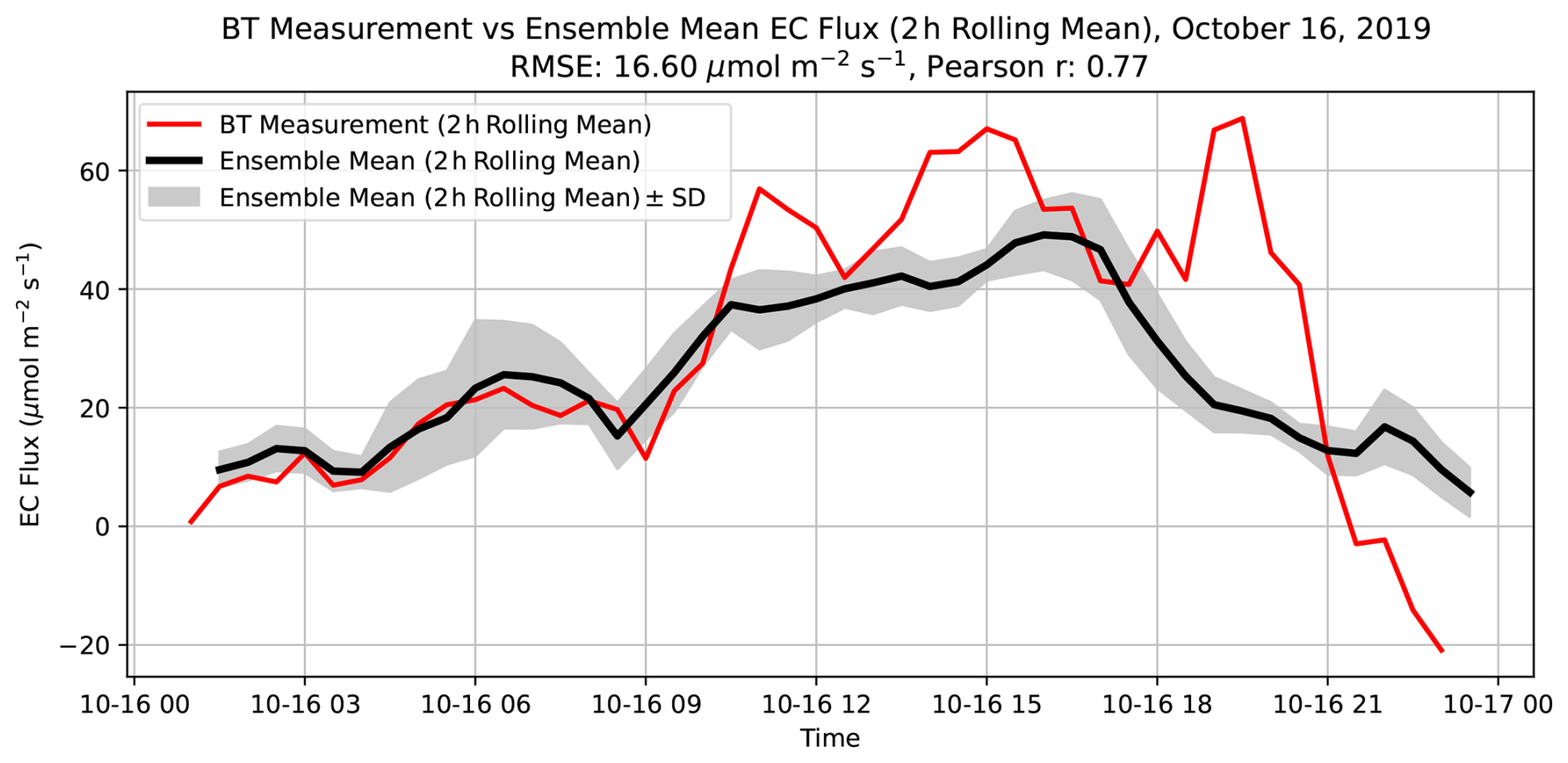
Figure 15Comparison of ensemble mean and BT tower measurement on 16 October 2019. Shaded area shows the standard deviation range of the ensemble.
At the same time, differences remain between the modelled and observed fluxes, particularly during periods when the measured half-hourly values show sharp excursions. Some of these discrepancies are reduced after temporal smoothing, which supports the interpretation that part of the disagreement in the single-realisation comparison arises from the stochastic nature of turbulence rather than from a systematic model error alone. However, the remaining differences also indicate that ensemble variability does not explain all mismatches between LES and observations. The residual mismatches can be due to uncertainties in the emission profiles of the particular day.
We developed PALM-CO2, a high-resolution urban carbon dioxide transport modelling framework based on an urban large-eddy simulation code, PALM. The model resolves CO2 transport at metre-scale resolution (down to 10 m) under realistic meteorological conditions and explicitly represents urban topography, including terrain, buildings, and vegetation types. A key novelty of PALM-CO2, is its fully coupled treatment of fine-scale atmospheric dynamics with spatially detailed anthropogenic and biogenic surface carbon fluxes, enabling the simulation of CO2 transport processes within the urban canopy layer that cannot be captured by coarser-scale models.
The model considers complex urban land surface carbon fluxes from both anthropogenic and biogenic activities. Anthropogenic CO2 emissions are prescribed at metre-scale resolution (i.e. 10 m) using a bottom-up disaggregation framework that integrates multiple urban data sources, including gas consumption statistics, building energy performance data, industrial point-source inventories, and road transport emissions. Biogenic CO2 fluxes are represented through the online implementation of the VPRM within PALM. VPRM dynamically computes net ecosystem exchange using PALM-resolved near-surface meteorological conditions and satellite-derived vegetation indices (EVI and LSWI), allowing for a physically consistent coupling between surface carbon exchange and resolved turbulence.
The model is validated against eddy-covariance flux and wind measurements from measurement site at BT tower. Within the urban case study domain, simulated turbulent CO2 fluxes and horizontal wind speeds show good agreement with observations from the BT Tower, where anthropogenic emissions dominate the measured signal. When July is excluded, the average RMSE and correlation coefficient for EC fluxes are 16.74 µmol m−2 s−1 and 0.74, respectively. The average RMSEs for wind speed and wind direction were 2.30 m s−1 and 37.50°, respectively, while the corresponding average correlation coefficients were 0.50 and 0.68. To further assess the biogenic component, PALM-CO2 is evaluated against flux measurements from the Lanžhot site in the Czech Republic, a deciduous forest ecosystem comparable to the green spaces in the Regent's Park in the study area. Simulated NEE captures both dormant and peak growing season behaviour well, while differences in the timing of budburst and senescence reflect climatic contrasts between the two regions, as also indicated by EVI and LSWI. The annual average biogenic flux of the Greater London Area is −3.95 kton d−1 in the model, close to the number in the ICOS-VPRM product −4.92 kton d−1. Annual cycle of biogenic flux agrees with the ICOS-VPRM product, with a correlation coefficient 0.97. These evaluations demonstrate the robustness of both the transport and surface flux components of PALM-CO2.
Overall, PALM-CO2 provides a physically consistent framework for simulating carbon dioxide transport in complex urban environments at metre-scale resolution. By explicitly resolving urban topography, atmospheric turbulence, and the coupled effects of anthropogenic and biogenic surface fluxes, the model captures multi-scale interactions that cannot be represented in coarser atmospheric transport models. The results demonstrate that fine-scale heterogeneity in emissions, land cover, and boundary-layer dynamics strongly influences urban CO2 distributions, particularly under stable conditions and during periods of shallow boundary-layer development. These findings underline the importance of high-resolution large-eddy simulation approaches for advancing process-level understanding of urban carbon dynamics and for improving the reliability of urban-scale carbon modelling. PALM-CO2 thus establishes a robust modelling foundation for future studies investigating urban carbon processes, emission attribution, and the role of cities in the regional carbon cycle.
Table A1 lists the sectors, sub-sectors and sub-subsectors used in the London Atmospheric Emission Inventory (London Datastore, 2023). Sub-sectors or sub-subsectors with no emissions have been excluded in the table. Some sub-subsectors have not shown in the table and merged (those of Rail and River).
Table A1Inventory source categories and GLA total emissions. NRMM = non-road mobile machinery.
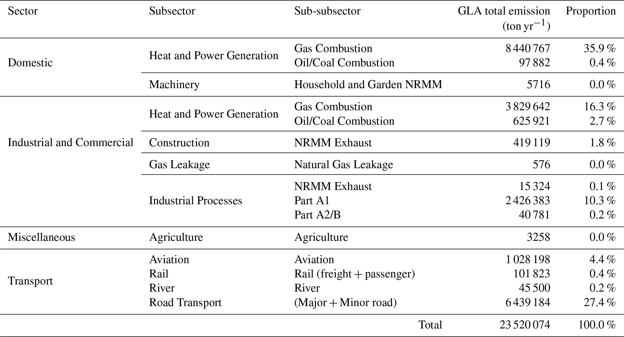
Results for all months are presented in Figs. B1, B2, and B3 for EC fluxes, wind speed, and wind direction respectively. The metrics are listed in Table B1.
Table B1Monthly performance metrics for EC flux, wind speed, and wind direction predictions. Root mean square error and correlation coefficient r are listed. Units are for RSMEs and biases. r has unit 1. Both simulation and BT tower measurement are on the 16th day of each month. Measurement is missing for 16 June.
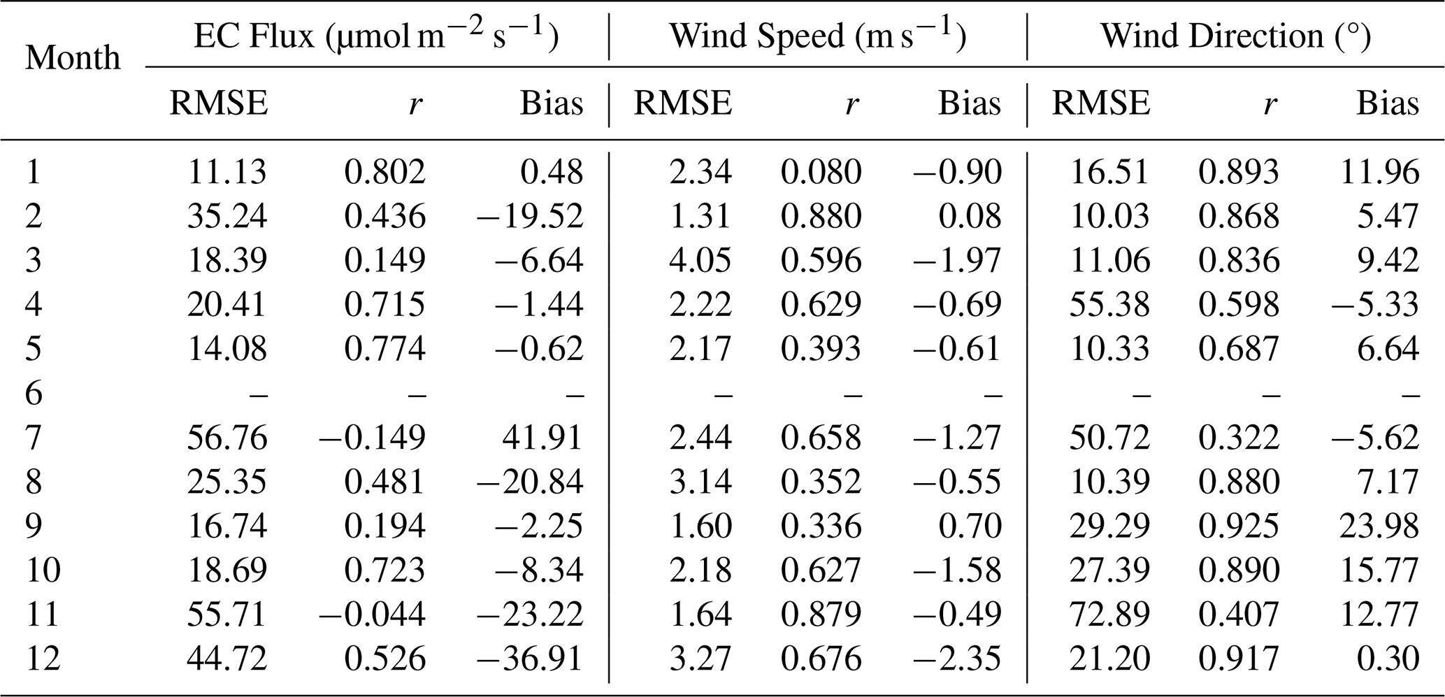
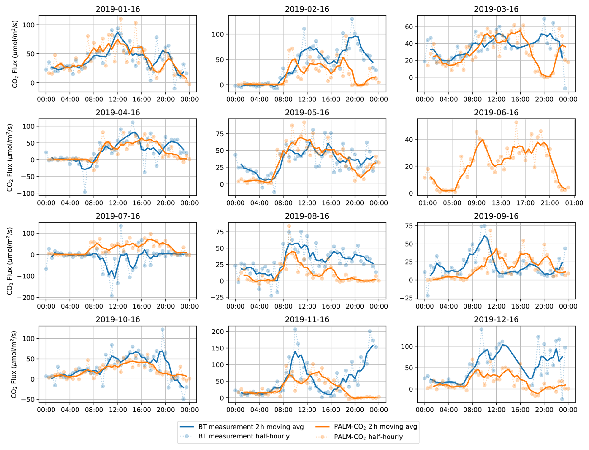
Figure B1Comparison of simulated and measured EC fluxes for all days. Sporadic missing values in BT tower measurement have been filled by linear interpolation. All day's data are missing for 16 June 2019.
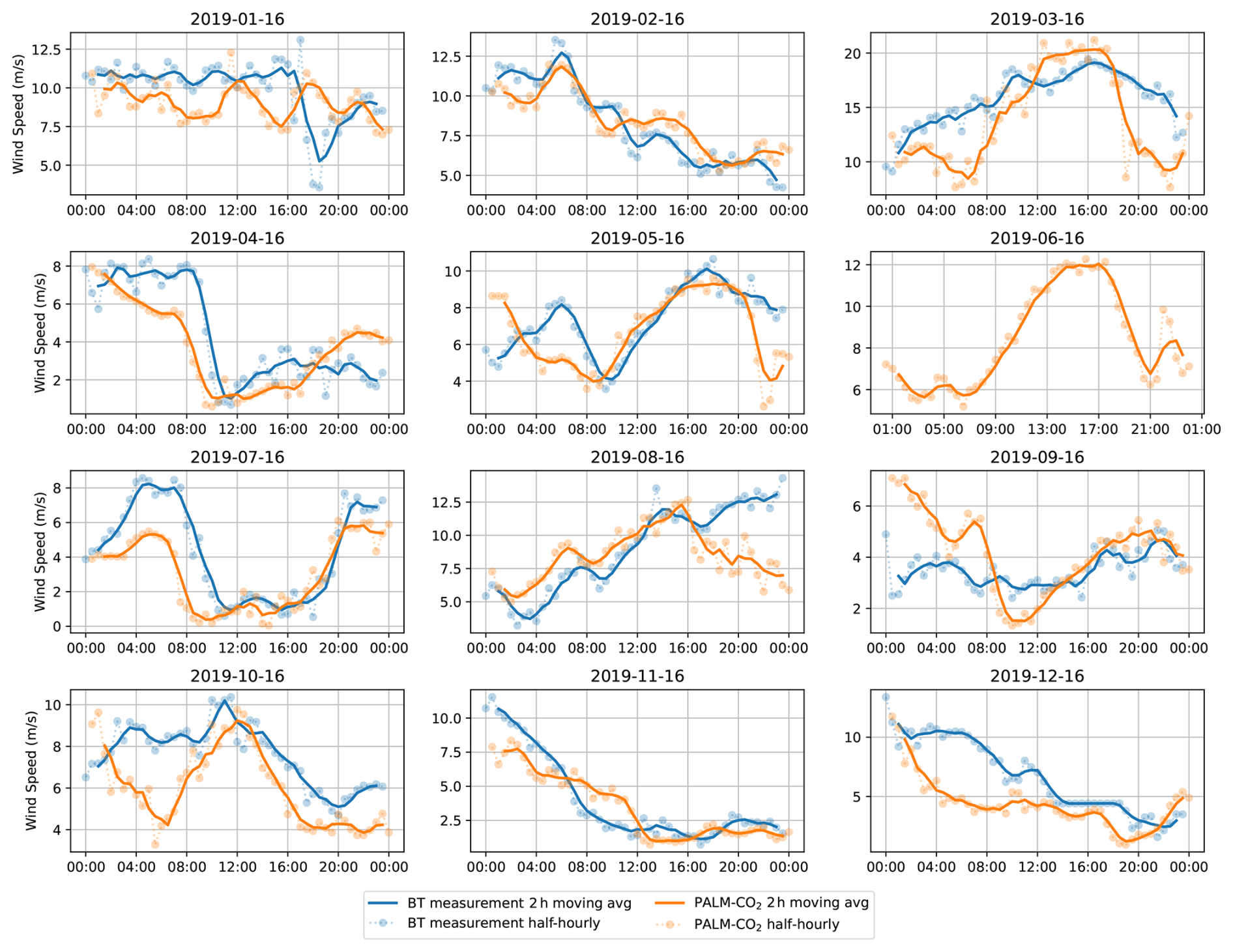
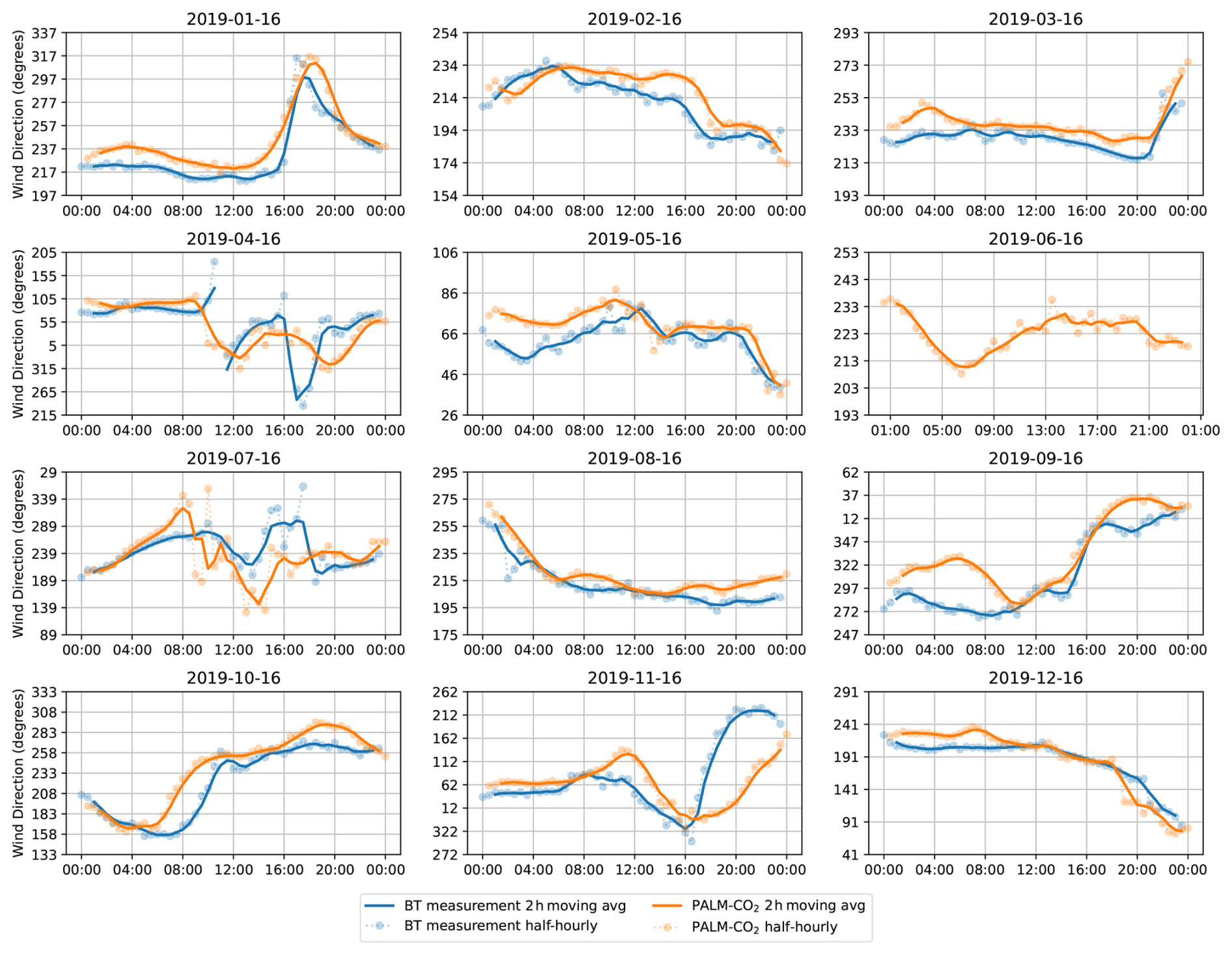
LES shows large over-estimate of EC flux on 16 July in Fig. 5. The reason is two-fold. First, the measurement on 16 July is not representative of a typical day in July. The processed EC flux data in the BT tower dataset have gone through quality control. The quality control checks several criteria including the magnitude of turbulence intensity, number of valid instantaneous measurements, out-of-range velocity ratios and range of heat fluxes. A quality control flag (qc) is provided in the dataset (Helfter et al., 2016). A qc value less than 2 is deemed good data. Figure C1 shows the BT measurement EC flux in July 2019 and their individual qc flag. It can be seen that from 16 July, quality of data deteriorated and more data are with qc flag = 2. The plot also shows the average 24 h EC flux profile for the first two weeks of July (1 to 14) as a blue line in the first day. This average profile is very different to that on 16 July. Therefore, it is likely the measurements on 16 July are unfortunately not representative of the real situation.
Another reason for the over-estimation in July is the small wind speed during morning peak hours on 16 July. As can be seen in Fig. 6 in main text, wind speed from 08:00 to 18:00 is very low even at 190 m height. At lower ground the wind speed would be even smaller. The worse convection condition will likely cause the build-up of flux in the domain that would otherwise be transported horizontally out of the domain. Eventually this caused an over-estimation.
To further prove this point, we select another day in July (the 20th) with moderate wind magnitude. This day has similar anthropogenic emission to 16 July. The results are plotted in Fig. C2. The simulated EC flux (blue lines in figure) is smaller, and smaller than that in January and October as expected. Comparison with observation is unreliable for 20 July due to bad data quality (orange lines in figure). However, if the average 24 h profile for the first two weeks of July (green lines in figure) is used in the comparison, the 20 July simulation is in good agreement with measurements (RMSE = 8.28 umol m−2 s−1, r= 0.819).
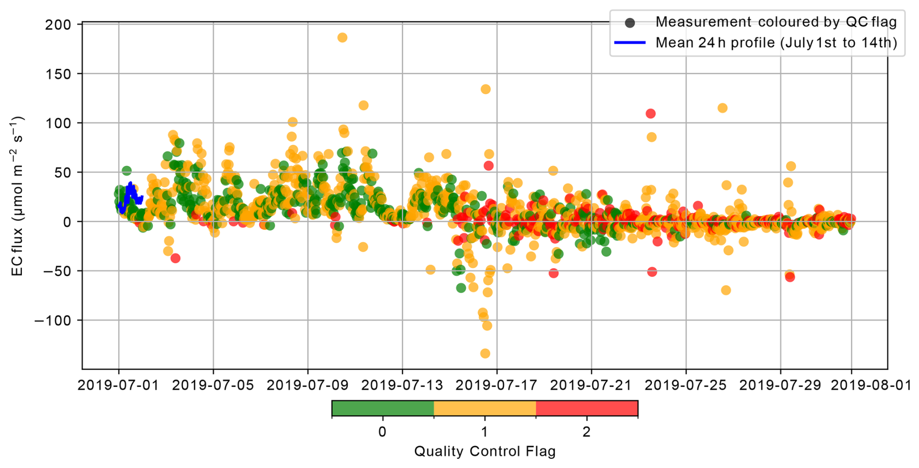
Figure C1BT measurement and quality control flag for July 2019. Individual half-hourly EC flux data points are coloured with quality flag. Less than 2 means good quality.
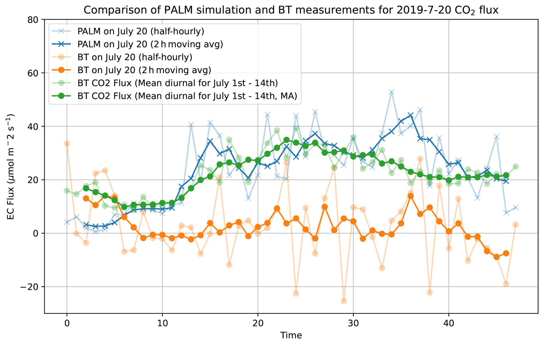
Figure C2Comparison of EC flux from LES and from measurement on 20 July. Due to poor quality of measurement on 20 July, the average EC flux profile of 1 to 14 July are plotted in green for comparison.
Two approaches are used to process LES results for EC flux as introduced in Sect. 3.4. The comparison of the two approaches are shown in Fig. D1. The plot shows that most of the times the two approaches generate same results. The small discrepancies in some hours might be due to under-resolved turbulent transport which is missing in the temporal averaging approach.
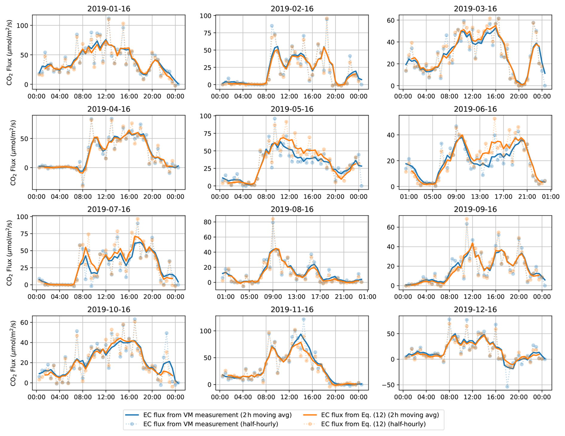
As stated in the main text, the grid sensitivity study was done on a smaller 2 km by 2 km area in Camden, London. Figure E1 shows the topography of the area in the 10 and 5 m resolution grid. The rasterisation can remove some low buildings and fill in holes in the topography where one single fluid grid is surrounded by solid grids. Figure E2 shows the constant emission patterns applied to the bottom surface of the computational domain. In case of grid in buildings, the emission is applied to the top of the building.
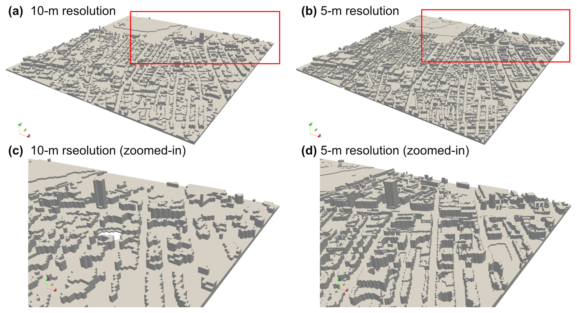
Figure E1Buildings and terrain heights after rasterisation to 10 and 5 m resolution.
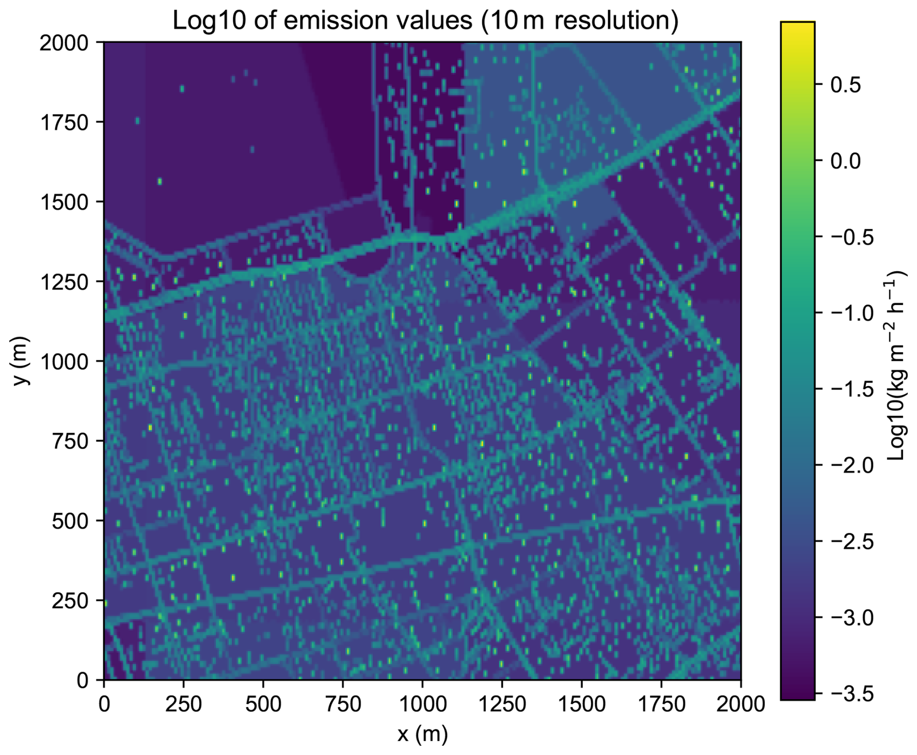
Figure E2Emission pattern used in the grid sensitivity study. A constant emission grid-map in time is used. The same pattern is used for both 10 and 5 m simulations. In 5 m simulation, the emission grid-map is interpolated bi-linearly from 10 to 5 m resolution.
Table F1 lists all the parameters used in the VPRM module in this study. It is a set of parameters fit for Europe (Lian et al., 2021).
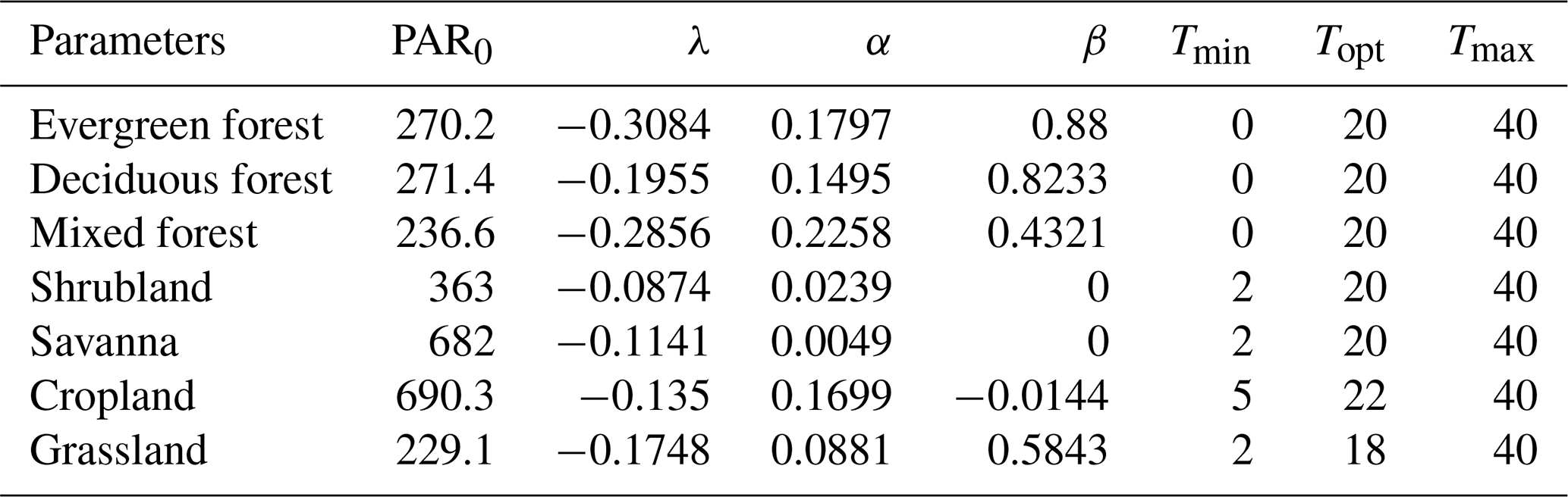
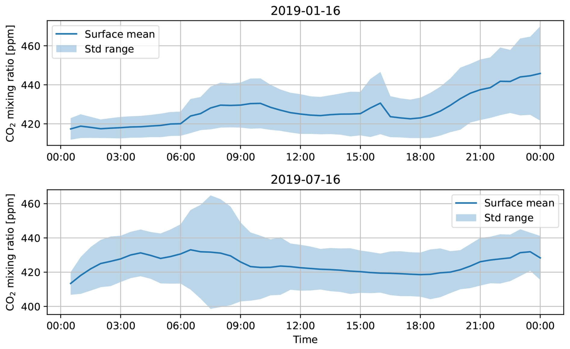
The exact version of the model used to produce the results used in this paper is archived on Zenodo repository under https://doi.org/10.5281/zenodo.18852193 under GPLv3 License (Li et al., 2026).
All input data are either open accessed or proprietary as listed in Table 2. All output data are available upon requests, since file size is too large to be openly hosted.
Conceptualization: LL, JZ, FF. Data curation: LL, JZ, FF. Funding acquisition: FF. Investigation: LL, FF. Methodology: LL, FF. Project administration: FF. Software: LL, FF. Validation: LL. Visualization: LL. Writing (original draft preparation): LL. Writing (review and editing): LL, FF.
The contact author has declared that none of the authors has any competing interests.
Publisher's note: Copernicus Publications remains neutral with regard to jurisdictional claims made in the text, published maps, institutional affiliations, or any other geographical representation in this paper. The authors bear the ultimate responsibility for providing appropriate place names. Views expressed in the text are those of the authors and do not necessarily reflect the views of the publisher.
This work used the ARCHER2 UK National Supercomputing Service (https://www.archer2.ac.uk, last access: 15 July 2026). Authors thank Dr. Carole Helfter for her help in retrieving BT tower measurement data. We would like to thank the editor and reviewers for the in-depth comments that contributed to improving the presentation of our paper.
This research has been supported by the Engineering and Physical Sciences Research Council (grant no. EP/X029093/1).
This paper was edited by Mohamed Salim and reviewed by two anonymous referees.
Ahmadov, R., Gerbig, C., Kretschmer, R., Koerner, S., Neininger, B., Dolman, A., and Sarrat, C.: Mesoscale covariance of transport and CO2 fluxes: Evidence from observations and simulations using the WRF-VPRM coupled atmosphere-biosphere model, J. Geophys. Res.-Atmos., 112, https://doi.org/10.1029/2007JD008552, 2007. a
Ahmadov, R., Gerbig, C., Kretschmer, R., Körner, S., Rödenbeck, C., Bousquet, P., and Ramonet, M.: Comparing high resolution WRF-VPRM simulations and two global CO2 transport models with coastal tower measurements of CO2, Biogeosciences, 6, 807–817, https://doi.org/10.5194/bg-6-807-2009, 2009. a
An, X., Zhu, T., Wang, Z., Li, C., and Wang, Y.: A modeling analysis of a heavy air pollution episode occurred in Beijing, Atmos. Chem. Phys., 7, 3103–3114, https://doi.org/10.5194/acp-7-3103-2007, 2007. a
Anav, A., Friedlingstein, P., Kidston, M., Bopp, L., Ciais, P., Cox, P., Jones, C., Jung, M., Myneni, R., and Zhu, Z.: Evaluating the land and ocean components of the global carbon cycle in the CMIP5 earth system models, J. Climate, 26, 6801–6843, https://doi.org/10.1175/JCLI-D-12-00417.1, 2013. a
Anders, J. and Maronga, B.: Urban microscale simulations based on a Local Climate Zone wizard: Concept and validation using the PALM model system, Urban Climate, 63, 102576, https://doi.org/10.1016/j.uclim.2025.102576, 2025. a
Belda, M., Benešová, N., Resler, J., Huszár, P., Vlček, O., Krč, P., Karlický, J., Juruš, P., and Eben, K.: FUME 2.0 – Flexible Universal processor for Modeling Emissions, Geosci. Model Dev., 17, 3867–3878, https://doi.org/10.5194/gmd-17-3867-2024, 2024. a
Brunner, D., Kuhlmann, G., Marshall, J., Clément, V., Fuhrer, O., Broquet, G., Löscher, A., and Meijer, Y.: Accounting for the vertical distribution of emissions in atmospheric CO2 simulations, Atmos. Chem. Phys., 19, 4541–4559, https://doi.org/10.5194/acp-19-4541-2019, 2019. a, b
Cai, M., Ren, C., Shi, Y., Chen, G., Xie, J., and Ng, E.: Modeling spatiotemporal carbon emissions for two mega-urban regions in China using urban form and panel data analysis, Sci. Total Environ., 857, 159612, https://doi.org/10.1016/j.scitotenv.2022.159612, 2023. a
Chen, W., Wang, Y., Li, J., Yi, Z., Zhao, Z., Guo, B., Che, H., and Zhang, X.: Description and evaluation of a newly developed emission inventory processing system (EMIPS), Sci. Total Environ., 870, 161909, https://doi.org/10.1016/j.scitotenv.2023.161909, 2023. a
Christen, A., Coops, N., Crawford, B., Kellett, R., Liss, K., Olchovski, I., Tooke, T., Van Der Laan, M., and Voogt, J.: Validation of modeled carbon-dioxide emissions from an urban neighborhood with direct eddy-covariance measurements, Atmos. Environ., 45, 6057–6069, https://doi.org/10.1016/j.atmosenv.2011.07.040, 2011. a, b, c
Copernicus Atmosphere Monitoring Service: CAMS global greenhouse gas reanalysis (EGG4), Copernicus Atmosphere Monitoring Service (CAMS) Atmosphere Data Store [data set], https://doi.org/10.24381/cda4ed31, 2021. a, b
Crippa, M., Solazzo, E., Huang, G., Guizzardi, D., Koffi, E., Muntean, M., Schieberle, C., Friedrich, R., and Janssens-Maenhout, G.: High resolution temporal profiles in the Emissions Database for Global Atmospheric Research, Scientific Data, 7, 121, https://doi.org/10.1038/s41597-020-0462-2, 2020. a
Department for Energy Security and Net Zero: Lower and Middle Super Output Areas Gas Consumption, https://www.gov.uk/government/statistics/lower-and-middle-super-output-areas-gas-consumption (last access: 15 July 2026), 2015. a, b
Department for Levelling Up, Housing & Communities: Energy Performance of Buildings Data: England and Wales, https://epc.opendatacommunities.org/ (last access: 15 July 2026), 2025. a, b
Dhakal, S.: GHG emissions from urbanization and opportunities for urban carbon mitigation, Curr. Opin. Env. Sust., 2, 277–283, https://doi.org/10.1016/j.cosust.2010.05.007, 2010. a
Duchemin, B., Goubier, J., and Courrier, G.: Monitoring phenological key stages and cycle duration of temperate deciduous forest ecosystems with NOAA/AVHRR data, Remote Sens. Environ., 67, 68–82, https://doi.org/10.1016/S0034-4257(98)00067-4, 1999. a
Environment Agency: National LIDAR Programme, Environment Agency [data set], https://www.data.gov.uk/dataset/f0db0249-f17b-4036-9e65-309148c97ce4/national-lidar-programme (last access: 15 July 2026), 2025. a, b
European Space Agency (ESA): Harmonized Sentinel-2 MSI: MultiSpectral Instrument, Level-2A (SR), https://developers.google.com/earth-engine/datasets/catalog/COPERNICUS_S2_SR_HARMONIZED (last access: 15 July 2026), 2025. a
Fenech, S., Doherty, R. M., Heaviside, C., Vardoulakis, S., Macintyre, H. L., and O'Connor, F. M.: The influence of model spatial resolution on simulated ozone and fine particulate matter for Europe: implications for health impact assessments, Atmos. Chem. Phys., 18, 5765–5784, https://doi.org/10.5194/acp-18-5765-2018, 2018. a
Friedlingstein, P., O'Sullivan, M., Jones, M. W., Andrew, R. M., Bakker, D. C. E., Hauck, J., Landschützer, P., Le Quéré, C., Luijkx, I. T., Peters, G. P., Peters, W., Pongratz, J., Schwingshackl, C., Sitch, S., Canadell, J. G., Ciais, P., Jackson, R. B., Alin, S. R., Anthoni, P., Barbero, L., Bates, N. R., Becker, M., Bellouin, N., Decharme, B., Bopp, L., Brasika, I. B. M., Cadule, P., Chamberlain, M. A., Chandra, N., Chau, T.-T.-T., Chevallier, F., Chini, L. P., Cronin, M., Dou, X., Enyo, K., Evans, W., Falk, S., Feely, R. A., Feng, L., Ford, D. J., Gasser, T., Ghattas, J., Gkritzalis, T., Grassi, G., Gregor, L., Gruber, N., Gürses, Ö., Harris, I., Hefner, M., Heinke, J., Houghton, R. A., Hurtt, G. C., Iida, Y., Ilyina, T., Jacobson, A. R., Jain, A., Jarníková, T., Jersild, A., Jiang, F., Jin, Z., Joos, F., Kato, E., Keeling, R. F., Kennedy, D., Klein Goldewijk, K., Knauer, J., Korsbakken, J. I., Körtzinger, A., Lan, X., Lefèvre, N., Li, H., Liu, J., Liu, Z., Ma, L., Marland, G., Mayot, N., McGuire, P. C., McKinley, G. A., Meyer, G., Morgan, E. J., Munro, D. R., Nakaoka, S.-I., Niwa, Y., O'Brien, K. M., Olsen, A., Omar, A. M., Ono, T., Paulsen, M., Pierrot, D., Pocock, K., Poulter, B., Powis, C. M., Rehder, G., Resplandy, L., Robertson, E., Rödenbeck, C., Rosan, T. M., Schwinger, J., Séférian, R., Smallman, T. L., Smith, S. M., Sospedra-Alfonso, R., Sun, Q., Sutton, A. J., Sweeney, C., Takao, S., Tans, P. P., Tian, H., Tilbrook, B., Tsujino, H., Tubiello, F., van der Werf, G. R., van Ooijen, E., Wanninkhof, R., Watanabe, M., Wimart-Rousseau, C., Yang, D., Yang, X., Yuan, W., Yue, X., Zaehle, S., Zeng, J., and Zheng, B.: Global Carbon Budget 2023, Earth Syst. Sci. Data, 15, 5301–5369, https://doi.org/10.5194/essd-15-5301-2023, 2023. a, b, c
Gerbig, C. and Koch, F.-T.: Biosphere-atmosphere exchange fluxes for CO2 from the Vegetation Photosynthesis and Respiration Model VPRM for 2006–2022, , ICOS [data set], https://doi.org/10.18160/VX78-HVA1, 2021. a, b
Gerbig, C. and Koch, F.-T.: Biosphere-atmosphere exchange fluxes for CO2 from the Vegetation Photosynthesis and Respiration Model VPRM for 2022–2023, ICOS [data set], https://doi.org/10.18160/R5HS-YKW0, 2024. a
Guevara, M., Tena, C., Porquet, M., Jorba, O., and Pérez García-Pando, C.: HERMESv3, a stand-alone multi-scale atmospheric emission modelling framework – Part 1: global and regional module, Geosci. Model Dev., 12, 1885–1907, https://doi.org/10.5194/gmd-12-1885-2019, 2019. a
Guevara, M., Jorba, O., Tena, C., Denier van der Gon, H., Kuenen, J., Elguindi, N., Darras, S., Granier, C., and Pérez García-Pando, C.: Copernicus Atmosphere Monitoring Service TEMPOral profiles (CAMS-TEMPO): global and European emission temporal profile maps for atmospheric chemistry modelling, Earth Syst. Sci. Data, 13, 367–404, https://doi.org/10.5194/essd-13-367-2021, 2021. a, b
Helfter, C., Famulari, D., Phillips, G. J., Barlow, J. F., Wood, C. R., Grimmond, C. S. B., and Nemitz, E.: Controls of carbon dioxide concentrations and fluxes above central London, Atmos. Chem. Phys., 11, 1913–1928, https://doi.org/10.5194/acp-11-1913-2011, 2011. a, b, c
Helfter, C., Tremper, A. H., Halios, C. H., Kotthaus, S., Bjorkegren, A., Grimmond, C. S. B., Barlow, J. F., and Nemitz, E.: Spatial and temporal variability of urban fluxes of methane, carbon monoxide and carbon dioxide above London, UK, Atmos. Chem. Phys., 16, 10543–10557, https://doi.org/10.5194/acp-16-10543-2016, 2016. a, b, c, d
Hersbach, H., Bell, B., Berrisford, P., Hirahara, S., Horányi, A., Muñoz-Sabater, J., Nicolas, J., Peubey, C., Radu, R., Schepers, D., Simmons, A., Soci, C., Abdalla, S., Abellan, X., Balsamo, G., Bechtold, P., Biavati, G., Bidlot, J., Bonavita, M., De Chiara, G., Dahlgren, P., Dee, D., Diamantakis, M., Dragani, R., Flemming, J., Forbes, R., Fuentes, M., Geer, A., Haimberger, L., Healy, S., Hogan, R. J., Hólm, E., Janisková, M., Keeley, S., Laloyaux, P., Lopez, P., Lupu, C., Radnoti, G., de Rosnay, P., Rozum, I., Vamborg, F., Villaume, S., and Thépaut, J.-N.: The ERA5 global reanalysis, Q. J. Roy. Meteor. Soc., 146, 1999–2049, https://doi.org/10.1002/qj.3803, 2020. a, b
Heus, T., van Heerwaarden, C. C., Jonker, H. J. J., Pier Siebesma, A., Axelsen, S., van den Dries, K., Geoffroy, O., Moene, A. F., Pino, D., de Roode, S. R., and Vilà-Guerau de Arellano, J.: Formulation of the Dutch Atmospheric Large-Eddy Simulation (DALES) and overview of its applications, Geosci. Model Dev., 3, 415–444, https://doi.org/10.5194/gmd-3-415-2010, 2010. a
ICOS RI, Aalto, J., Aiguier, T., Alivernini, A., Aluome, C., Andersson, T., Arriga, N., Aurela, M., Back, J., Barten, S., Baur, T., Bazot, S., Beauclair, P., Becker, N., Becker, N., Belelli Marchesini, L., Bergström, G., Bernhofer, C., Berveiller, D., Biermann, T., Bloor, J., Bodson, B., Bogaerts, G., Bortoli, M., Bosio, I., Brut, A., Brümmer, C., Buchmann, N., Buysse, P., Båth, A., Calandrelli, D., Cavagna, M., Ceschia, E., Chabbi, A., Chebbi, W., Chianucci, F., Chipeaux, C., Chopin, H., Claverie, N., Cobbe, I., Colosse, D., Conte, A., Corsanici, R., Courtois, P., Coyle, M., Crill, P., Cuntz, M., Cuocolo, D., Czerný, R., DEPUYDT, J., Darenová, E., Darsonville, O., De Ligne, A., De Meulder, T., De Simon, G., Decau, M.-L., Dell'Acqua, A., Delorme, J.-P., Delpierre, N., Demoulin, L., Denou, J.-L., Di Matteo, B., Di Tommasi, P., Dienstbach, L., Dignam, R., Dolfus, D., Domec, J.-C., Douxfils, B., Dufrêne, E., Dumont, B., Durand, B., Eichelmann, U., Engelmann, T., Esposito, A., Esser, O., Etzold, S., Eugster, W., Famulari, D., Fares, S., Faurès, A., Feigenwinter, I., Feldmann, I., Fincham, W., Fischer, M., Foltýnová, L., Friborg, T., Galliot, J.-N., Garcia Quiros, I., Garrigou, C., Gasbarra, D., Gessler, A., Gharun, M., Gianelle, D., Gimper, S., Goded, I., Graf, A., Granouillac, F., Grenier, M., Grudd, H., Grünwald, T., Guillot, T., Harvey, D., Hatakka, J., Haustein, A., Hehn, M., Heinesch, B., Helfter, C., Heliasz, M., Holst, J., Holst, T., Hug, C., Häni, M., Hörtnagl, L., Ibrom, A., Ilardi, F., Jackowicz-Korczynski, M. A., Janssens, I., Jensen, R., Jocher, G., Joetzjer, E., Jones, M., Kempf, J., Kettler, M., Kljun, N., Klumpp, K., Kolari, P., Korrensalo, A., Kowalska, N., Kozii, N., Krejza, J., Kristoffersson, A., Kruijt, B., Kruszewski, A., Kumar, S., Kummer, S., Laakso, H., Lafont, S., Lange Rønn, E., Larmanou, E., Laurila, T., Leeson, S., Lefevre, L., Lehner, I., Lemaire, B., Levula, J., Levy, P., Liechti, K., Lily, J.-B., Limousin, J.-M., Linderson, M.-L., Lindgren, K., Lohila, A., Longdoz, B., Lootens, R., Loubet, B., Loustau, D., Lundin, E., López-Blanco, E., Löfvenius, P., Magliulo, V., Mammarella, I., Manco, A., Manise, T., Marcolla, B., Marek, M. V., Marklund, P., Marloie, O., Martin, R., Martin Saint Paul, N., Marty, M., Matilainen, T., Mattes, J., Matteucci, M., Mauder, M., Meier, P., Meire, A., Meis, J., Mensah, C., Michaud, L., Minerbi, S., Moderow, U., Montagnani, L., Moretti, V., Morfin, A., Mullinger, N., Mäkelä, T., Männikkö, M., Männistö, E., Mölder, M., Møller, F., Naiken, A., Naseer, M., Nemitz, E., Nezval, O., Nilsson, M., Orgun, A., Ottosson-Löfvenius, M., Ourcival, J.-M., Paasch, S., Pavelka, M., Peichl, M., Perot-Guillaume, C., Perrot, C., Pihlatie, M., Pilegaard, K., Piret, A., Prasse, H., Pumpanen, J., Rainne, J., Rakos, N., Rasmussen, L., Rebmann, C., Rinne, J., Rodeghiero, M., Roland, M., Rudd, D., Røjle Christensen, T., Schaarup Sørensen, J., Schmidt, M., Schmidt, P., Schmitt Oehler, M., Schrader, F., Segers, J., Simioni, G., Smith, P., Snellen, H., Sorgi, T., Soudani, K., Staník, K., Staudinger, M., Stecher, M., Stutz, T., Suopajärvi, S., Sutter, F., Taipale, R., Tallec, T., Tenca, F., Thimonier Rickenmann, A., Thyrion, T., Tomelleri, E., Tosca, M., Trotsiuk, V., Trusina, J., Tuittila, E.-S., Tuovinen, J.-P., Tyssandier, J., Tülp, H., Van Look, J., Varjonen, S., Vesala, T., Vescovo, L., Vincent, G., Vincke, C., Vitale, L., Vágner, L., Waldner, P., Wiesen, R., Winck, B., Yeung, K., Zampedri, R., Zawilski, B., Zenone, T., Zimmermann, S., Zweifel, R., van Dijk, N., van der Molen, M., Öquist, M., Šigut, L., Šlížek, J., and ICOS ETC: Ecosystem final quality (L2) product in ETC-Archive format – INTERIM release 2023-2, ICOS [data set], https://doi.org/10.18160/JYAR-7YEH, 2023. a, b
Intergovernmental Panel on Climate Change: Climate Change 2023: Synthesis Report, Contribution of Working Groups I, II and III to the Sixth Assessment Report of the Intergovernmental Panel on Climate Change, IPCC, https://doi.org/10.59327/IPCC/AR6-9789291691647, 2023. a
Jähn, M., Kuhlmann, G., Mu, Q., Haussaire, J.-M., Ochsner, D., Osterried, K., Clément, V., and Brunner, D.: An online emission module for atmospheric chemistry transport models: implementation in COSMO-GHG v5.6a and COSMO-ART v5.1-3.1, Geosci. Model Dev., 13, 2379–2392, https://doi.org/10.5194/gmd-13-2379-2020, 2020. a
Järvi, L., Havu, M., Ward, H. C., Bellucco, V., McFadden, J. P., Toivonen, T., Heikinheimo, V., Kolari, P., Riikonen, A., and Grimmond, C. S. B.: Spatial modeling of local-scale biogenic and anthropogenic carbon dioxide emissions in Helsinki, J. Geophys. Res.-Atmos., 124, 8363–8384, https://doi.org/10.1029/2018JD029576, 2019. a, b
Jiang, S., Wang, J., Li, C., Ou, J., Duan, P., and Li, L.: Identification of no-fly zones for delivery drone path planning in various urban wind environments, Phys. Fluids, 36, https://doi.org/10.1063/5.0221281, 2024. a
Khan, B., Banzhaf, S., Chan, E. C., Forkel, R., Kanani-Sühring, F., Ketelsen, K., Kurppa, M., Maronga, B., Mauder, M., Raasch, S., Russo, E., Schaap, M., and Sühring, M.: Development of an atmospheric chemistry model coupled to the PALM model system 6.0: implementation and first applications, Geosci. Model Dev., 14, 1171–1193, https://doi.org/10.5194/gmd-14-1171-2021, 2021. a
Li, L., Zheng, J., and Fang, F.: PALM-CO2 (v01), Zenodo [code], https://doi.org/10.5281/zenodo.18852193, 2026. a, b
Li, Y., Henze, D. K., Jack, D., and Kinney, P. L.: The influence of air quality model resolution on health impact assessment for fine particulate matter and its components, Air Qual. Atmos. Hlth., 9, 51–68, https://doi.org/10.1007/s11869-015-0321-z, 2016. a
Lian, J., Bréon, F.-M., Broquet, G., Lauvaux, T., Zheng, B., Ramonet, M., Xueref-Remy, I., Kotthaus, S., Haeffelin, M., and Ciais, P.: Sensitivity to the sources of uncertainties in the modeling of atmospheric CO2 concentration within and in the vicinity of Paris, Atmos. Chem. Phys., 21, 10707–10726, https://doi.org/10.5194/acp-21-10707-2021, 2021. a, b, c
Lin, D., Zhang, J., Khan, B., Katurji, M., and Revell, L. E.: GEO4PALM v1.1: an open-source geospatial data processing toolkit for the PALM model system, Geosci. Model Dev., 17, 815–845, https://doi.org/10.5194/gmd-17-815-2024, 2024. a
London Datastore: London Atmospheric Emissions Inventory (LAEI) 2019, London Datastore [data set], https://data.london.gov.uk/dataset/london-atmospheric-emissions-inventory-laei-2019-e758q/ (last access: 15 July 2026), 2023. a, b, c, d
Mahadevan, P., Wofsy, S. C., Matross, D. M., Xiao, X., Dunn, A. L., Lin, J. C., Gerbig, C., Munger, J. W., Chow, V. Y., and Gottlieb, E. W.: A satellite-based biosphere parameterization for net ecosystem CO2 exchange: Vegetation Photosynthesis and Respiration Model (VPRM), Global Biogeochem. Cy., 22, https://doi.org/10.1029/2006GB002735, 2008. a, b
Marcotullio, P. J., Sarzynski, A., Albrecht, J., Schulz, N., and Garcia, J.: The geography of global urban greenhouse gas emissions: An exploratory analysis, Climatic Change, 121, 621–634, https://doi.org/10.1007/s10584-013-0977-z, 2013. a
Maronga, B., Banzhaf, S., Burmeister, C., Esch, T., Forkel, R., Fröhlich, D., Fuka, V., Gehrke, K. F., Geletič, J., Giersch, S., Gronemeier, T., Groß, G., Heldens, W., Hellsten, A., Hoffmann, F., Inagaki, A., Kadasch, E., Kanani-Sühring, F., Ketelsen, K., Khan, B. A., Knigge, C., Knoop, H., Krč, P., Kurppa, M., Maamari, H., Matzarakis, A., Mauder, M., Pallasch, M., Pavlik, D., Pfafferott, J., Resler, J., Rissmann, S., Russo, E., Salim, M., Schrempf, M., Schwenkel, J., Seckmeyer, G., Schubert, S., Sühring, M., von Tils, R., Vollmer, L., Ward, S., Witha, B., Wurps, H., Zeidler, J., and Raasch, S.: Overview of the PALM model system 6.0, Geosci. Model Dev., 13, 1335–1372, https://doi.org/10.5194/gmd-13-1335-2020, 2020. a, b, c, d
Neves, T., Fisch, G., and Raasch, S.: Local convection and turbulence in the Amazonia using large eddy simulation model, Atmosphere, 9, 399, https://doi.org/10.3390/atmos9100399, 2018. a
Ordnance Survey (GB): OS MasterMap Building Height Attribute, EDINA Digimap Ordnance Survey Service [CSV geospatial data], https://digimap.edina.ac.uk (last access: 15 July 2026), 2019a. a, b, c
Ordnance Survey (GB): OS MasterMap Topography Layer, EDINA Digimap Ordnance Survey Service [GeoPackage geospatial data], https://digimap.edina.ac.uk (last access: 15 July 2026), 2019b. a, b, c
Ordnance Survey (GB): OS Terrain 50, EDINA Digimap Ordnance Survey Service [ASC geospatial data], https://digimap.edina.ac.uk (last access: 15 July 2026), 2019c. a, b
Pfafferott, J., Rißmann, S., Sühring, M., Kanani-Sühring, F., and Maronga, B.: Building indoor model in PALM-4U: indoor climate, energy demand, and the interaction between buildings and the urban microclimate, Geosci. Model Dev., 14, 3511–3519, https://doi.org/10.5194/gmd-14-3511-2021, 2021. a
Pillai, D., Gerbig, C., Marshall, J., Ahmadov, R., Kretschmer, R., Koch, T., and Karstens, U.: High resolution modeling of CO2 over Europe: implications for representation errors of satellite retrievals, Atmos. Chem. Phys., 10, 83–94, https://doi.org/10.5194/acp-10-83-2010, 2010. a
Pillai, D., Gerbig, C., Ahmadov, R., Rödenbeck, C., Kretschmer, R., Koch, T., Thompson, R., Neininger, B., and Lavrié, J. V.: High-resolution simulations of atmospheric CO2 over complex terrain – representing the Ochsenkopf mountain tall tower, Atmos. Chem. Phys., 11, 7445–7464, https://doi.org/10.5194/acp-11-7445-2011, 2011. a
Skamarock, W. C., Klemp, J. B., Dudhia, J., Gill, D. O., Liu, Z., Berner, J., Wang, W., Powers, J. G., Duda, M. G., Barker, D. M., and Huang, X.-Y.: A description of the advanced research WRF version 4, NCAR Tech. Note NCAR/TN-556+ Str, 145, figshare, https://doi.org/10.6084/m9.figshare.7369994.v4, 2019. a, b
Smith, A. C., Li, L., Xiang, J., and Fang, F.: Machine learning-based land-use regression models for predicting carbon dioxide concentrations in San Francisco Bay area, Environ. Earth Sci., 84, 539, https://doi.org/10.1007/s12665-025-12582-w, 2025. a
Stagakis, S., Brunner, D., Li, J., Backman, L., Karvonen, A., Constantin, L., Järvi, L., Havu, M., Chen, J., Emberger, S., and Kulmala, L.: Intercomparison of biogenic CO2 flux models in four urban parks in the city of Zurich, Biogeosciences, 22, 2133–2161, https://doi.org/10.5194/bg-22-2133-2025, 2025. a
Stroh, E., Harrie, L., and Gustafsson, S.: A study of spatial resolution in pollution exposure modelling, Int. J. Health Geogr., 6, 19, https://doi.org/10.1186/1476-072x-6-19, 2007. a
Wilby, R. L. and Perry, G. L.: Climate change, biodiversity and the urban environment: a critical review based on London, UK, Prog. Phys. Geog., 30, 73–98, https://doi.org/10.1191/0309133306pp470ra, 2006. a
Wood, C., Lacser, A., Barlow, J. F., Padhra, A., Belcher, S. E., Nemitz, E., Helfter, C., Famulari, D., and Grimmond, C.: Turbulent flow at 190 m height above London during 2006–2008: a climatology and the applicability of similarity theory, Bound.-Lay. Meteorol., 137, 77–96, https://doi.org/10.1007/s10546-010-9516-x, 2010. a, b
Zanaga, D., Van De Kerchove, R., Daems, D., De Keersmaecker, W., Brockmann, C., Kirches, G., Wevers, J., Cartus, O., Santoro, M., Fritz, S., Lesiv, M., Herold, M., Tsendbazar, N.-E., Xu, P., Ramoino, F., and Arino, O.: ESA WorldCover 10 m 2021 v200, Zenodo [data set], https://doi.org/10.5281/zenodo.7254221, 2022. a, b
We published the code under the name PALM-CO2 (Li et al., 2026) yet we intend to merge the developed modules with the main PALM code in the future.
This emission coefficient for domestic gas consumption is from DESNZ report Greenhouse gas reporting: conversion factors 2019 – Natural gas fuel, and has been tweaked to match to total annual emission of the sub-subsector in the LAEI region.
This emission coefficient for non-domestic gas consumption is from Department for Energy Security and Net Zero report Greenhouse gas reporting: conversion factors 2019 – Natural gas fuel.
- Abstract
- Introduction
- Model description: PALM-CO2
- Case Study and Experimental Setup
- Results and discussion
- Conclusions
- Appendix A: Sectors and subsectors in emission inventory
- Appendix B: Results for all months
- Appendix C: Additional analysis for 16 July
- Appendix D: EC flux processing procedure
- Appendix E: Additional information on grid sensitivity study
- Appendix F: VPRM parameters
- Appendix G: Diurnal cycles of surface CO2 concentration
- Code availability
- Data availability
- Author contributions
- Competing interests
- Disclaimer
- Acknowledgements
- Financial support
- Review statement
- References
- Abstract
- Introduction
- Model description: PALM-CO2
- Case Study and Experimental Setup
- Results and discussion
- Conclusions
- Appendix A: Sectors and subsectors in emission inventory
- Appendix B: Results for all months
- Appendix C: Additional analysis for 16 July
- Appendix D: EC flux processing procedure
- Appendix E: Additional information on grid sensitivity study
- Appendix F: VPRM parameters
- Appendix G: Diurnal cycles of surface CO2 concentration
- Code availability
- Data availability
- Author contributions
- Competing interests
- Disclaimer
- Acknowledgements
- Financial support
- Review statement
- References