EXSoDOS 1.0: downscaling of weather extremes shifts for ensemble climate projections using ground-based measurements, reanalysis and stochastic modelling

Accurately representing the changes of local extreme weather events in climate projections is crucial for climate impact assessment and adaptation services. Climate models do no explicitly represent these events as observed by weather stations due to their coarse spatial resolution. Existing downscale products successfully reduce overall biases of past or future climatological variables, but the representation of variability and extreme events including their past and future shifts under climate change are still not addressed. A new stochastic model, EXSoDOS, addresses this gap by the DOwnScaling of weather EXtremes Shifts for ensemble climate projections using ground-based measurements, reanalysis, and global climate models. This is done by using a stochastic model that correlates coarse-scale gridded historical climate records with the point-scale measurements. Therefore, EXSoDOS combines ground-based data (either from the Global Historical Climatological Network or user-specified), ERA5 (ECMWF Re-Analysis 5), and GCM (global climate model) projections from CMIP6 (Coupled Model Intercomparison Project Phase 6) to downscale past and future daily climate records. We demonstrate EXSoDOS for 5 use cases, resp. daily minimum temperature in Belgium, daily maximum temperature in Azerbaijan, heat stress in India, wind velocity in Germany and precipitation in Mali. It is found that EXSoDOS is able to represent annual cycle variability, density distributions, and extreme events of return periods of up to 10 years, while they are all underrepresented by the raw GCM outputs. Observed tendencies towards more extremes between two past periods 1961–1990 and 1991–2020 are also better represented. Projections under the SSP585 scenario suggest amplified extremes in maximum temperature, precipitation, and heat stress by 2071–2100. Furthermore, downscaling affects the outcomes of shifting extremes under future climate change, which is evident in terms of both absolute and relative changes, as well as changes in return periods. While limitations of statistical downscaling persist, it is concluded that EXSoDOS offers a novel method for estimating past and future shifts in weather extremes for weather stations with a sufficient daily record of data of multiple decades.

1 Introduction

Global (Eyring et al., 2016) and regional (Katragkou et al., 2024; Coppola et al., 2021) climate model initiatives have been succesful in predicting many aspects of climate change, like increasing temperature and shifts in precipitation amounts. However, events like heavy precipitation, heavy wind, extreme heat (stress) and cold spells as observed by (point-scale) weather stations are not explicitly represented in climate projections. This results from a scale mismatch between coarse spatial resolution of GCMs and point-scale observations for which the scale of the extreme events are too small to be resolved (IPCC, 2021; Fischer and Knutti, 2015; Sillmann et al., 2013). Particularly, meteorological point-scale observations generally show much more erratic temporal variability than the coarser-scale gridded products. Especially, extreme precipitation and wind, but also temperature and heat stress, can be influenced by confounding local climate effects resulting in local features like local convective precipitation events and urban heat islands. However, local extreme weather events have large impacts on society, infrastructure and ecosystems. Hence, their underrepresentation hampers extreme hazard assessment and their impacts under climate change. Not only the absolute representation but also the shifts of extreme weather distributions under past and future climate change are crucial for climate risk assessment and adaptation planning (IPCC, 2023).

Several techniques have been developed to downscale global (Eyring et al., 2016) and regional (Katragkou et al., 2024; Coppola et al., 2021) climate projections to represent their small-scale climate effects. On the one hand, they include mechanistic downscaling using convection permitting atmospheric numerical models with a resolution of 7 km down to 1 km (Kendon et al., 2021), high enough to resolve deep convection and associated extreme precipitation (Vanden Broucke et al., 2019; Brisson et al., 2016) and local land use like urban areas (Wouters et al., 2016; De Ridder et al., 2015). they have been effective to project extreme weather events (Fosser et al., 2024; Termonia et al., 2018; Wouters et al., 2017; Saeed et al., 2017). On the other hand, statistical downscaling methods have been developed (Maraun, 2016) to finer grids of 0.5° (e.g., ISIMIP3BASD by Lange, 2019) and 1km resolution (e.g., CHELSA-W5E5 by Karger et al., 2023) and point observation locations (Switanek et al., 2022), whereas GCM resolutions are ∼ 1–3°. Finally, a downscaling method to estimate the probability parameters and return values was recently proposed by Benestad et al. (2025), which can be used as input to weather generators.

However, future climate assessment of local extremes is hampered by the requirements of computatational resources and input data requirements. Particularly, mechanistic downscaling with atmospheric numerical models are computationally very demanding since higher-resolution climate also requires smaller integration time step becacuse of the courant-frederich-levichs criterium (Prein et al., 2015). The most recent point-location stochastic downscaling models (Switanek et al., 2022; Volosciuk et al., 2017; Devis et al., 2013) and weather generators (Van De Velde et al., 2023; Brisson et al., 2015) have only applied to specific areas or variables, or have not been applied to future climate projections. Gridded downscaling products may either have a low resolution (Lange, 2019) or do not cover ensemble future climate either (Karger et al., 2023). While these different downscaling products can reduce overall biases of coarse-scale time series, their representation of extremes in terms of variability, distributions and their return periods as observed from weather stations are not addressed, let stand the shifts under past and future climate change. A downscaling method that represents past and future shifts in probability distributions and return levels according to observations and that is simultaneously constrained to time series from model members of climate projections doesn't exist yet.

To fill this gap, we present EXSoDOS, a DOwnScaling method of weather EXtremes Shifts for climate projections using ground-based measurements, reanalysis, global climate models, and statistical downscaling. It downscales time series from an ensemble of global climate models to represent the variability and extremes as observed by weather stations. The model implements a stochastic downscaling technique that is calibrated on point-scale observations and coarse-scale reanalysis, with over 84 years of climate historical climate data (from 1940 to present). Hereby, historical coarse-scale reanalysis data and observations are normalized and correlated with each other. This is done by mapping predictor and predictand values to standard normal space using their empirical CDFs (i.e., apply the probability integral transform and then the inverse normal CDF), acquiring correlation in that space, and finally mapping back sampled values through the inverse empirical CDF of observations.

While its stochastic downscaling approach builds on established perfect-prognosis concepts, the novelty of EXSoDOS lies in its ability to evaluate shifts in local weather extremes across past and future climatological periods for different variables. This is achieved by the combined use of (1) globally available long-term datasets including weather station observations, ERA5 (ECMWF Re-Analysis 5; Hersbach et al., 2020), and the GCM (global climate model) ensemble from CMIP6 (Coupled Model Intercomparison Project Phase 6; Eyring et al., 2016), (2) a non-parametric treatment of distributions, and a (3) workflow that allows direct comparison of observed, reconstructed, and projected extremes. Its end-to-end design makes consistent assessment of extreme-event variability and return levels across multiple decades, and variables for any climate region possible.

The method can be used at locations where longterm records (60 years) of observations are available. It can either employ observational data from the Global Historical Climate Network (GHCN) hosted by the National Oceanic and Atmospheric Administration (NOAA; https://www.ncei.noaa.gov/products/land-based-station/global-historical-climatology-network-daily, last access: 8 June 2026), or ingest data from local observational sources, e.g., measurements carried out by national meteorological offices, agro-meteorological or environmental institutes. In the case of the latter, one only requires the position (in latitude longitude coordinates) and the observed time series in a commonly used format (csv or parquet). The stochastic model is then applied on multi-member climate projections towards 2100 after bias-correcting them with reanalysis data. As such, the method follows the downscaling strategy proposed by Switanek et al. (2022), and is further designed to represent climate extremes regarding different weather variables including daily minimum and maximum temperature, heat stress temperature and wind speed. To evaluate the representation of extreme events with respect to observations and their shifts under past and future climate change, a number of statistics are employed, including the daily-to-annual variability, density distributions and overlaps, and return periods.

EXSoDOS runs quickly and automatically. For a single station, a full downscaling run for one scenario typically takes ∼ 5–10 s, and a 10-member ensemble completes in <1 min on a modern CPU, excluding one-time data download and gridded bias-adjustment preprocessing. Downloading of source data (ERA5, CMIP6 climate models, station data) can take longer (network dependent) and quantile-delta mapping (QDM) bias-adjustment (incl. ERA5 grid upscaling) on continental grids can take hours, which is performed once per model/grid.

EXSoDOS can be applied at locations where a sufficiently extensive record of observations from weather stations are available, preferably 60 years of continuous data record or longer. It is also easily applicable by requiring only a few parameters, particularly the station coordinates, the weather time series under scope (either temperature, precipitation, wind, or heat stress). The synthesis of time series for a handful of stations and a handful of climate model members and climate scenarios takes less than an hour on a contemporary desktop computer, resulting in a negligible carbon footprint of computer resources. Our service is demonstrated for several specific use cases across the globe, in which the statistical model is calibrated and validated on historical data, and applied on climate projections. The demonstration is featured by metrics common to extremes climate assessment, including annual cycles, density distributions and return periods.

The structure of the remaining of this paper is as follows. In Sect. 2, the program interface with global data sources, the downscaling procedure, and bias correction are described. The statistics for validation and assessment as well as the case areas are described after. In Sect. 3, we perform a validation of the model output for the historical period, and the assessment with climate projections for each of the use cases. We conclude the paper with perspectives and challenges for extreme weather assessment under climate change in Sect. 4.

2 Method

To perform the downscaling, coarse-scale predictors (x) are correlated to the point-scale predictands (y). Calibration and validation of the statistical model is done on the basis of historical reanalysis reconstruction x_r and the measurements from the weather stations y_o. While ensemble models of climate projections offer the statistical climate properties on the multi-annual time series including anomalies, they are not in synchrony with observations or, in other words, their sequence of weather patterns generally differ from that of the observations. Consequently, they cannot be used to correlate the coarse-scale model output with local measurements. Therefore, historical reanalysis, which is constrained and in synchrony with the observations, is used for the calibration. For calibration, half of the days in the time series are chosen randomly for calibration ($x_{\mathrm{r}}^{\mathrm{c}}$, $y_{\mathrm{o}}^{\mathrm{c}}$) and the other half for validation ($x_{\mathrm{r}}^{\mathrm{v}}$, $y_{\mathrm{o}}^{\mathrm{v}}$). We used a 50 : 50 split, because we require that the overall distribution and extremes to be represented on a climatological timescale in both calibration and validation. Over a 60-year period we have an equivalent of 30-year data for both, which is in line with climatology assessment standards of the World Meteorological Organization (WMO, 2017). Finally, the downscaling is applied on the climate model projections x.

To ensure scale consistency of the predictors between calibration phase and application phase, the climate reanalysis is upscaled to the climate model grid for each individual model. Furthermore, the downscaling procedure follows the perfect prognosis assumption (Maraun, 2016), which means that the predictor is describing the reality free from biases. Therefore, the biased predictors from the climate models (x_b) are bias-adjusted with a quantile-delta mapping procedure (Cannon et al., 2015), see also Sect. 2.3. The downscaling strategy above leads to the following subsequent steps, see also Fig. 1:

1. Acquire climate reconstruction (reanalysis) and upscale to the climate model grid by aggregation and interpolation

2. Acquire historical predictand (y_o) from weather stations

3. Extract historical predictor (x_r) from upscaled reanalysis at point locations of the weather stations

4. Randomly select half of the historical data for model calibration ($x_{\mathrm{r}}^{\mathrm{c}}$ and $y_{\mathrm{r}}^{\mathrm{c}}$) and the remaining half for model validation ($x_{\mathrm{r}}^{\mathrm{c}}$ and $y_{\mathrm{r}}^{\mathrm{c}}$)

5. calibration of the statistical model using x^c and y^c (Sect. 2.2)

6. Validation of the statistical model using $x_{\mathrm{r}}^{\mathrm{v}}$ and comparing the output with $y_{\mathrm{r}}^{\mathrm{v}}$, see Sect. 2.4)

7. Acquire (biased) climate projections for point locations (x_b)

8. Climate projections are bias-adjusted (indicated with x_m) with upscaled reanalysis using quantile-delta mapping, Sect. 2.3)

9. Synthesis of downscaled climate projections (y_m) by applying the statistical model on bias-adjusted climate projections (Sect. 2.5)

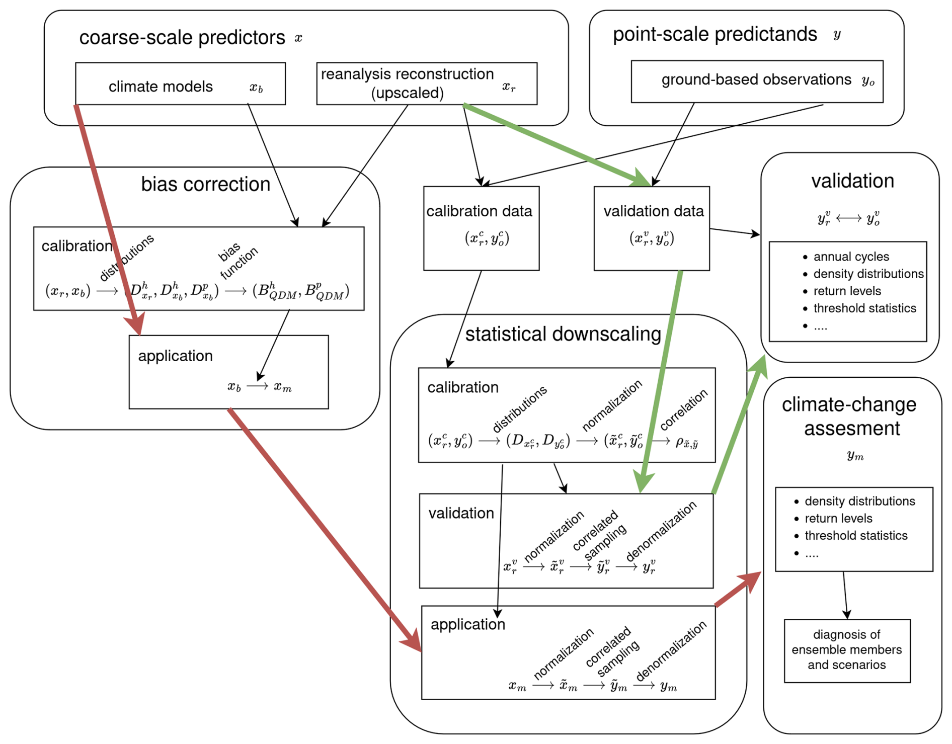
Figure 1 Overview of EXSoDOS. The green arrows indicate the validation steps starting from the reanalysis reconstruction, whereas the red arrows indicate the assessment steps starting from the climate models.

As such, the procedure performs bias-adjustment at the coarse scales and statistical downscaling towards the point scale in separate steps. This avoids inconsistencies arising from mixing up statistical properties (particularly, quantile values) across spatial scales. The latter could occur if one would apply the statistical downscaling directly on the climate model output without bias-adjustment on the grid level. Especially, trends under climate change including those of the (extreme) quantile values at the local scales can differ to those (spatially aggregated) at the coarse scales, so these should not be used for one another. As shown by Maraun (2013), mapping point-scale quantiles to coarse-scale quantiles, or vice versa, may lead to unrealistic trends of extremes leading to misinterpretation. The strategy of scale separation where scale transition is established with a statistical model only after bias-adjustment at the model grid level is in accordance to previous methods (Lange, 2019; Switanek et al., 2022; Volosciuk et al., 2017), and advised by previous analyses (Maraun, 2013). The key assumptions of EXSoDOS include (see also Table S1 in the Supplement):

1. Realism of bias-adjusted coarse scale predictors (perfect prognosis assumption),

2. Stationarity of predictor–predictand correlations,

3. Stochastic representation of subgrid variability,

4. Sufficient record length of observations to represent extremes up to ∼ 10-year return periods,

5. QDM bias-adjustment stationarity (Cannon et al., 2015) and

6. Independence across stations and variables.

The different processing steps are implemented in Python and computationally optimized as vectorized numerical operations with Python Xarray, Pandas and NumPy.

In the next subsections, we elaborate the input data sets, the statistical downscaling and bias-adjustment in more detail.

2.1 Input

A key design feature of EXSoDOS is the consistent use of datasets with hyper-climatological temporal coverage (> 60 years), which enables robust estimation of variability and extremes as well as their shifts between climatological periods. By relying exclusively on globally available datasets (ERA5, CMIP6, and station observations), the framework is fully transferable to any station location where a sufficiently long record of observations exists, including data-sparse regions such as Mali.

Observations collected from GHCN are used as predictand for calibration and validation. It includes 10 010 stations for which it reports an available record of at least 60 years, see Fig. 2. The minimum record length needs to be 60 years. On the one hand, the 60 year record is required to provide sufficient data for both calibration and validation. As a 50 : 50 split is applied, an equivalent of 30 years of data is available for both calibration and validation, which is in line climatology assessment standards of the World Meteorological Organization (WMO, 2017). On the other hand, one can address 2×30 years of records to evaluate the model performance to capture past shifts in weather extremes driven by global climate models. One should only use records with observational records covering ≥ 90 % of the sample period. We do not infill gaps: missing values are treated as NaN and excluded from empirical CDF correlation construction. Alternatively, the service is able to read observational data provided by the user in a common format (csv, parquet, netcdf) for which one specifies their station coordinates (as elaborated by one of the use cases, see Sect. 2.6.2).

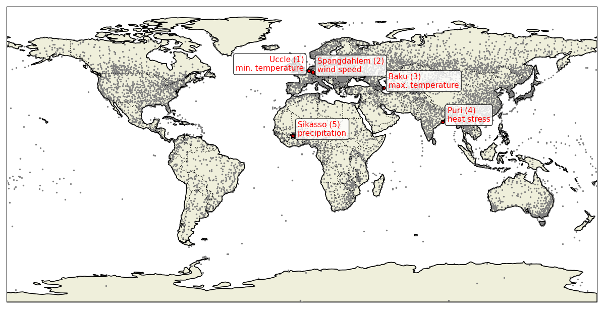
Figure 2 The 10 010 stations from the global historical network (grey dots) of with it reports at least 30 years of data within the time span 1940–2023. EXSoDOS use cases for each of the variables provided by the global network are indicated as red circles and provided a user-input data as star for Sikasso (Mali).

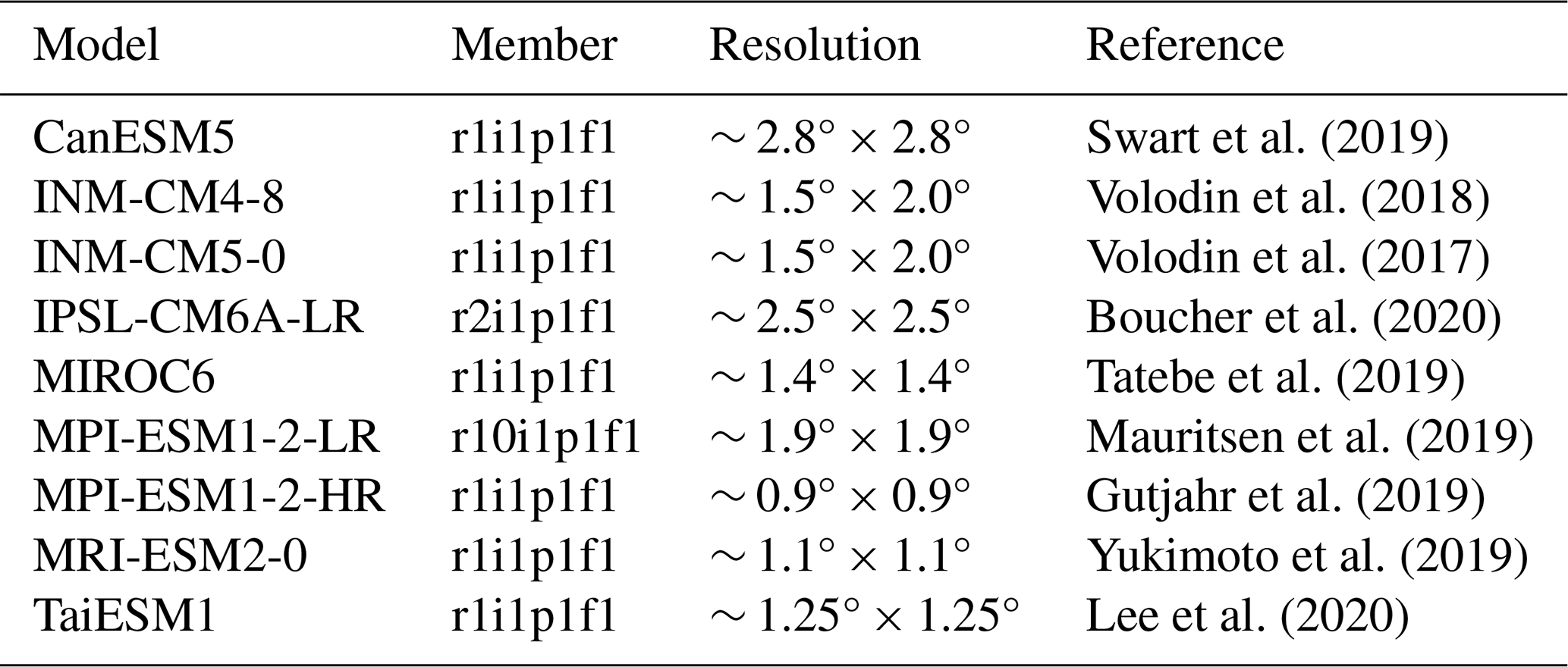
Next, ERA5 (Hersbach et al., 2020) is used as reanalysis climate reconstruction for the coarse-scale predictor x_r. ERA5 reanalysis covers more than 80 years of data from 1940 until now that can be used for calibration and validation of the statistical model, hence suitable to build a robust statistical relation between predictor and predictand. Finally, the climate model ensemble members of the Coupled Model Intercomparison Project Phase 6 (CMIP6) see (Eyring et al., 2016) from 1931 up to 2100 are used as predictor input for EXSoDOS to generate and assess downscaled daily time series from past to future climate. These are downloaded from one of the data nodes of the Earth System Grid Federation (ESGF), see https://esgf.llnl.gov/ (last access: 8 June 2026). For demonstration of EXSoDOS, 9 models listed in the Table 1 are used, but the user can specify any other combination of model members available at ESGF.

Swart et al. (2019)Volodin et al. (2018)Volodin et al. (2017)Boucher et al. (2020)Tatebe et al. (2019)Mauritsen et al. (2019)Gutjahr et al. (2019)Yukimoto et al. (2019)Lee et al. (2020)

Table 1 Climate models and references used in this study from the 6th phase of the Coupled Model Intercomparison Project (CMIP6), see Eyring et al. (2016).

2.2 Statistical downscaling

The stochastic downscaling strategy follows the general philosophy of perfect-prognosis and analog-based approaches previously proposed in the literature (e.g., Volosciuk et al., 2017; Switanek et al., 2022). EXSoDOS does not introduce a fundamentally new class of stochastic models; instead, it adapts and extends these approaches within a unified framework that is explicitly designed for multi-decadal extreme-event assessment across historical and future climates.

The basic model strategy is to randomly sample point-scale predictands (y) from measurements in such a way that they are correlating with coarse-scale predictors (x), as proposed by Switanek et al. (2022). As such, the predictors can be extracted from climate projection and then used as input for the model to generate future point-scale time series including future extreme values. The current method is now reformulated to work not only with precipitation but also with other climate parameters, including temperature, wind speed and heat stress. This is done by performing the normalizing and denormalization steps with a non-parametric distributions. We further improve the model by implementing different predictor classes of different magnitude. Additionally, we implement a rescaling step of the point-scale predictand with the coarse-scale predictor before applying the stochastic model, which leads to improved results on high extremes in case of precipitation and wind speed (see Sect. 3.1 for results). For the sake of clarity, we elaborate the details of the statistical model in the subections below.

2.2.1 Stochastic model

A statistical relationship between x and y is established for each month separately. Calibration is performed per calendar month. To increase sample size, and providing smooth transition between months while preserving seasonal representativeness, we include data from the adjacent months (±1 month), yielding an effective 3-month seasonal window. A sensitivity test using single-month windows showed sligthly less robust tail estimates due to reduced calibration sample size per month (not shown).

Afterwards, to allow the relation between the predictor and predictand to be dependent on the magnitude of the predictor, the sample data is subdivided into a number of categories (n=3) of different magnitudes of the predictor percentiles. In the case of temperature and heat stress, the category bins of equal sample size are constructed, for which their boundaries are determined by equidistant values of the cumulative distribution function p(x):

$$\begin{array}{}\text{(1)}& p_i=i/n\mathrm{for}\mathrm{0}\le i\le n\end{array}$$

In the case of precipitation and wind speed, daily distributions have large tails, which we want to represent in the stochastic model. We use an exponential profile for quantiles of category borders which provides more categories in the tails, hence to cover the large variation in the tails of the distributions:

$$\begin{array}{}\text{(2)}& p_i=\left\{\begin{array}{ll}\mathrm{1}-\exp \left(l_i\right)& \mathrm{for}\mathrm{0}\le i\le n-\mathrm{1}\\ \mathrm{1}& \mathrm{for}i=n\end{array}\right.\end{array}$$

where

$$\begin{array}{}\text{(3)}& l_i=i\ln \left(f_{\max }\right)/(n-\mathrm{1})\mathrm{for}\mathrm{0}\le i\le n-\mathrm{1}\end{array}$$

are equidistant values for i going from 0 to n−1, and ln (f_max) is the logarithm of the (prescribed) chance (that is, frequency f_max)) for the observation to fall in the upper bin. As such, $p_{n-\mathrm{1}}=\mathrm{1}-f_{\max }$ represents the lower quantile border of that the upper bin. The exponential profile (note that ln (f_max) is negative hence also p_i) leads to more categories in the tails. Finally, the quantile categories q_i are calculated from the quantile function q_D of the calibration data $x_{\mathrm{r}}^{\mathrm{c}}$ of the historical period (h):

$$\begin{array}{}\text{(4)}& q_i=q_{{\mathrm{D}}_{x_{\mathrm{r}}^{\mathrm{c}}}^h}\left(p_i\right)\end{array}$$

Here above and throughout this manuscript, we follow the notation of Maraun (2016). For each of these categories, the predictand is correlated with the predictor variable. At first, the predictor and predictands are normalized within each category for the calibration data:

$$\begin{array}{}\text{(5)}& {\displaystyle }{\stackrel{\mathrm{̃}}{x}}_{\mathrm{r}}^{\mathrm{c}}=q_{\mathrm{N}}\left(p_{{\mathrm{D}}_{x_{\mathrm{r}}^{\mathrm{c}}}}\left(x_{\mathrm{r}}^{\mathrm{c}}\right)\right)\text{(6)}& {\displaystyle }{\stackrel{\mathrm{̃}}{y}}_{\mathrm{o}}^{\mathrm{c}}=q_{\mathrm{N}}\left(p_{{\mathrm{D}}_{y_{\mathrm{o}}^{\mathrm{c}}}}\left(y_{\mathrm{o}}^{\mathrm{c}}\right)\right)\end{array}$$

where $p_{{\mathrm{D}}_{x_{\mathrm{r}}^{\mathrm{c}}}}$ and $p_{{\mathrm{D}}_{y_{\mathrm{r}}^{\mathrm{c}}}}$ are the cumulative distribution functions of the the calibration predictor $x_{\mathrm{r}}^{\mathrm{c}}$ and predictand $y_{\mathrm{o}}^{\mathrm{c}}$, and q_N the quantile function of the normal distribution.

Subsequently, the correlation between the normalized predictor and normalized predictand is estimated from ${\stackrel{\mathrm{̃}}{x}}_{\mathrm{r}}^{\mathrm{c}}$ and ${\stackrel{\mathrm{̃}}{y}}_{\mathrm{o}}^{\mathrm{c}}$:

$$\begin{array}{}\text{(7)}& {\mathit{\rho }}_{\stackrel{\mathrm{̃}}{x}\stackrel{\mathrm{̃}}{y}}\simeq \langle {\stackrel{\mathrm{̃}}{x}}_{\mathrm{r}}^{\mathrm{c}}{\stackrel{\mathrm{̃}}{y}}_{\mathrm{o}}^{\mathrm{c}}\rangle \end{array}$$

where 〈⋅〉 indicates the average.

The normalized predictand is now sampled as a linear combination of normalized predictor and an extra random variable r as follows:

$$\begin{array}{}\text{(8)}& \stackrel{\mathrm{̃}}{y}=\mathit{\alpha }\stackrel{\mathrm{̃}}{x}+\mathit{\beta }\stackrel{\mathrm{̃}}{r}\end{array}$$

with

$$\begin{array}{}\text{(9)}& \stackrel{\mathrm{̃}}{x}=q_{\mathrm{N}}\left(p_{{\mathrm{D}}_{x_{\mathrm{r}}^{\mathrm{c}}}}\left(x\right)\right)\end{array}$$

the predictor normalized according to the estimated probability distribution function calculated above, and the predictor x can be either the upscaled reanalysis for validation $x_{\mathrm{r}}^{\mathrm{v}}$ or the bias-adjusted climate models x_m for the application (predictor from climate projections). One can obtain $\stackrel{\mathrm{̃}}{y}$ correlating with $\stackrel{\mathrm{̃}}{x}$ with a correlation coefficient ρ by setting α=ρ and $\mathit{\beta }=\sqrt{\mathrm{1}-{\mathit{\alpha }}^{\mathrm{2}}}$ (see Appendix A), hence

$$\begin{array}{}\text{(10)}& \stackrel{\mathrm{̃}}{y}=\mathit{\rho }\stackrel{\mathrm{̃}}{x}+\sqrt{\mathrm{1}-{\mathit{\rho }}^{\mathrm{2}}}\stackrel{\mathrm{̃}}{r}\end{array}$$

Finally, one can calculate the modeled predictand by inverting Eq. (6):

$$\begin{array}{}\text{(11)}& y=q_{{\mathrm{D}}_{y_{\mathrm{o}}^{\mathrm{c}}}}\left(p_{\mathrm{N}}\left(\stackrel{\mathrm{̃}}{y}\right)\right)\end{array}$$

where p_N is the cumulative distribution function of the Gaussian normal distribution and $q_{{\mathrm{D}}_{x^{\mathrm{c}}}}$ is again the quantile function of the calibration dataset.

In contrast to Switanek et al. (2022), the current method for (de)normalizing the variables is non-parametric, hence doesn't take any assumptions on particular statistical distributions (e.g., gamma distribution for precipitation or Weibull distribution for wind speed), hence any climate variable can be generated including precipitation, wind speed, temperature and heat stress, as long as the observation record is long enough to represent their density distributions.

2.2.2 Detrending of climate projections

In the description above, a statistical relationship (i.e., correlation through their normalized time series) is established between the predictor variable at the coarse scales and the predictand variable at the point scale. However especially in the case of temperature variables, distribution values in future climate at coarse scales exceed the range of the distribution of the historical period because of global warming. This leads to a cutoff for highest extremes, since they are all mapped to the highest observed value from the historical record. To overcome this problem and still represent the high extremes in future global warming, the predictor from the projections are detrended by dividing by the 30-year mean of the given month and multiplying it by its mean of the reference period 1986–2015 (in order to avoid division by zero in this operation and the problems arising from negative values, temperature variables are expressed in Kelvin). This is done before normalizing the predictor in Eq. (9). Afterwards, the sampled predictand from Eq. (11) is retrended by dividing again by the predictor mean of the reference period and multiplying with the 30-year mean. By performing these operations, the statistical relationship (correlation) between the coarse-scale and point-scale variables is now considered relative to their long-term averages, and it's assumed that it doesn't change under climate change. Correlation stability and stationarity of the statistical relationship under climate change and its effect on model results are assessed for daily precipitation in Sikasso in Text S1, Table S2 and Fig. S3 in the Supplement. It was found that the spread across simulations using 6 different calibration sets (even and odd years; 1961–2023, 1961–1990, 1991–2020) is of the same order as observation sampling sets (even vs. odd years; 1961–1990 vs. 1991–2020). The underlying correlation coefficient where also found to be stable. This indicates that statistical relationships are robust under climate change. Nevertheless, uncertainties arising from different calibration sets needs to be kept in mind in climate change assessments.

2.3 Bias-adjustment of climate projections

In the previous section, a statistical model is constructed and calibrated on on historical reanalysis data used as predictor variables and the point-scale weather observations. To apply the statistical model to the climate projections as predictor, the consistency with the historical reanalysis needs to be maximized. Therefore, the raw CMIP6 ensemble climate model data is bias-adjusted against the historical reanalysis data with quantile delta-mapping. The latter is based on the quantile-delta mapping described in Cannon et al. (2015). For the sake of clarity, we elaborate the QDM correction below, in which we also follow the notation of Maraun (2016).

The model bias B(p) is calculated as a function of the model's cumulative distribution function p (or “p”robabilities corresponding to a given model quantile) with respect to the climate reconstruction x_r and the “b”iased climate model output $x_{\mathrm{b}}^h$ in the historical overlapping timeframe (h) from 1961–2022:

$$\begin{array}{}\text{(12)}& B\left(p\right)=q_{{\mathrm{D}}_{x_{\mathrm{b}}}^h}\left(p\right)-q_{{\mathrm{D}}_{x_{\mathrm{r}}}^h}\left(p\right)\end{array}$$

This bias function determines the difference between the quantiles $q_{{\mathrm{D}}_{x_{\mathrm{b}}}^h}\left(p\right)$ of the climate model output and those of the climate reconstruction $q_{{\mathrm{D}}_{x_{\mathrm{r}}}^h}\left(p\right)$. For the historical period, the time series bias is then calculated as follows:

$$\begin{array}{}\text{(13)}& B_{\mathrm{QDM}}^h\left(x_{\mathrm{b},i}\right)=B\left(p_{{\mathrm{D}}_{x_{\mathrm{b}}}^h}\left(x_{\mathrm{b},i}\right)\right)\end{array}$$

from which can find the final bias-adjusted time series by subtracting the bias in the historical timeframe:

$$\begin{array}{}\text{(14)}& x_{\mathrm{m},i}=x_{\mathrm{b},i}-B_{\mathrm{QDM}}^h\left(x_{\mathrm{b},i}\right)\end{array}$$

for i a day in the historical time frame h (1991–2020). To create future bias-adjusted time series, quantile delta mapping assumes that the bias associated to each percentile B(p) (while changing the timeframe for calculating each percentile) is invariant under climate change. We get the following bias-adjustment function for the future timeframe p:

$$\begin{array}{}\text{(15)}& B_{\mathrm{QDM}}^p\left(x_{\mathrm{b},i}\right)=B\left(p_{{\mathrm{D}}_x^p}\left(x_{\mathrm{b},i}\right)\right)\end{array}$$

and:

$$\begin{array}{}\text{(16)}& x_{\mathrm{m},i}=x_{\mathrm{b},i}-B_{\mathrm{QDM}}^p\left(x_{\mathrm{b},i}\right)\end{array}$$

for i a day in the projected timeframe p with a 30-year timespan (e.g., 2071–2100). For a given day i, the timeframe for projection (p) is chosen in such a way that the day i is in the center of the timeframe. In practice, timeframes and the corresponding bias-adjustment function $B_{\mathrm{QDM}}^p$ are created in steps of five years, which is a compromise between computational cost and a smooth transition of bias-adjustment between the timeframes.

It can be verified that the cumulative density distribution of the climate model $\left(p_{{\mathrm{D}}_{x_i}^p}\right)$ is re-evaluated in the future period, which ensures that climate change signals of the quantile distribution is conserved. This is because the quantiles in the respective historical and future cumulative distributions p undergo the same bias-adjustment B(p), hence their difference remains conserved. This can be shown formerly by evaluating bias-adjustment (Eq. 16) on the quantiles $q_{{\mathrm{D}}_{x_{\mathrm{b}}}^p}\left(p\right)$ in the future timeframe:

$$\begin{array}{}\text{(17)}& \begin{array}{rcl}{q}_{{\mathrm{D}}_{x_{\mathrm{m}}^p}}\left(p\right)& =& q_{{\mathrm{D}}_{x_{\mathrm{b}}}^p}\left(p\right)-B_{\mathrm{QDM}}\left(q_{{\mathrm{D}}_{x_{\mathrm{b}}}^p}\left(p\right)\right)\\ & =& q_{{\mathrm{D}}_{x_{\mathrm{b}}}^p}\left(p\right)-B\left(p_{{\mathrm{D}}_{x_{\mathrm{b}}}^p}\left(q_{{\mathrm{D}}_{x_{\mathrm{b}}}^p}\left(p\right)\right)\right)\\ & =& q_{{\mathrm{D}}_{x_{\mathrm{b}}}^p}\left(p\right)-B\left(p\right)\end{array}\end{array}$$

and the bias-adjustment (Eq. 14) on the quantiles in the historical timeframe $q_{{\mathrm{D}}_{x_{\mathrm{b}}}^h}\left(p\right)$:

$$\begin{array}{}\text{(18)}& \begin{array}{rcl}{q}_{{\mathrm{D}}_{x_{\mathrm{m}}}^h}\left(p\right)& =& q_{{\mathrm{D}}_x^h}\left(p\right)-B_{\mathrm{QDM}}\left(q_{{\mathrm{D}}_x^h}\right(p\left)\right)\\ & =& q_{{\mathrm{D}}_x^h}\left(p\right)-B\left(p_{{\mathrm{D}}_x^h}\right(q_{{\mathrm{D}}_x^h}\left(p\right))\\ & =& q_{{\mathrm{D}}_x^h}\left(p\right)-B\left(p\right))\end{array}.\end{array}$$

Subtracting the two equations shows that the climate change signal on the quantiles are invariant for the QDM correction:

$$\begin{array}{}\text{(19)}& q_{{\mathrm{D}}_{x_{\mathrm{m}}^p}}\left(p\right)-q_{{\mathrm{D}}_{x_{\mathrm{m}}^h}}\left(p\right)=q_{{\mathrm{D}}_{x_{\mathrm{b}}}^p}\left(p\right)-q_{{\mathrm{D}}_{x_{\mathrm{b}}}^h}\left(p\right)\end{array}$$

Bias-adjustment of climate models are calculated over continental or global grids at once. To lower the computational cost and to obtain a more smooth bias-adjustment function, the bias is calculated for discrete values l of the cumulative distribution function p_l. As such, the bias function can be approximated as follows:

$$\begin{array}{}\text{(20)}& \begin{array}{rl}B\left(p\right)& \simeq \mathit{\alpha }\left(p\right)B\left(p_l\right)+(\mathrm{1}-\mathit{\alpha }(p\left)\right)B\left(p_{l+\mathrm{1}}\right),\\ & \mathrm{for}l\mathrm{where}{p}_l\le p<p_{l+\mathrm{1}}\end{array}\end{array}$$

with

$$\begin{array}{}\text{(21)}& \mathit{\alpha }=(q-q_l)/(q_{i+l}-q_l)\end{array}$$

As for the statistical model above, we consider equidistant discrete probability levels (in this case n=15) for temperature-like and heat-stress metrics (see Eq. 1), and an exponential profile for precipitation and wind speed (see Eq. 2) to represent their big tails. The time series $p_{{\mathrm{D}}_{x_{\mathrm{b}}}^p}\left(x_{\mathrm{b}}\right)$ are calculated from the model time series for each 5-year window and for each month separately, from which the bias at each timestep $B\left(p_{{\mathrm{D}}_{x_{\mathrm{b}}}^p}\right(x_{\mathrm{b}}\left)\right)$ can be evaluated using Eq. (20) and subtracted from the model output in Eq. (16).

As mentioned earlier, the climate models are generally coarser than the reference historical data, so the climate reconstruction (reanalysis data) is spatially aggregated to the coarser climate model grid. The bias may depend on the time of the year, hence the bias-adjustment B is calculated for each month of the year separately. Hereby, the bias of each month is calculated by considering the month before, the month itself and the month after.

2.4 Validation of variability and extremes

Downscaled time series (y^v) are generated by applying the statistical model on the coarse-scale reanalysis predictor ($x_{\mathrm{r}}^{\mathrm{v}}$) over a climatological historical period (1961–2023), and validated with station observations $y_{\mathrm{o}}^{\mathrm{v}}$. The validation focusses on the representation of the variability and extreme events. Therefore, their annual cycles, density distributions and return levels as a function of return period for the different datasets and timeframes are compared with the observations. For the annual cycles, the mean, median and 10th-to-90th percentile range of each day throughout the year is provided for highlighting the combined seasonality and variability of each variable throughout the year. Magnitude of extreme events are highlighted with density distributions, whereas occurrence of extreme events are highlighted with return levels as a function of return periods. Density distributions for all variables are weighted so that their integral sums to unity. This is except for precipitation for which the density is weighted with the average precipitation, in such a way that the integral sums to the average annual precipitation. The advantage of such a weighted density is that extreme precipitation values become more visible on the plots. Herewith, we report the overlap area between the different density distributions (Devis et al., 2013; Perkins et al., 2007):

$$\begin{array}{}\text{(22)}& S=\underset{-inf}{\overset{+inf}{\int }}min\left(\mathrm{PDF}\right(y_{\mathrm{v}}),{\mathrm{PDF}}^{\mathrm{o}}(y_{\mathrm{v}}\left)\right)\mathrm{d}{y}_{\mathrm{v}}\end{array}$$

While the Perkins distribution overlap score provides an integrated measure of similarity between two probability density functions, it is inherently insensitive to compensating errors and offers limited insight into discrepancies in the distribution tails. Therefore, we complement the Perkins score with additional distribution diagnostics, including quantile-based loss metrics, Kolmogorov–Smirnov statistics, and explicit indicators of extremes such as high percentiles, return levels (value as a function of return period, see below), and dry-day frequencies. These metrics are represented in a table and provide a comprehensive and objective assessment of both the central tendencies and the extreme behavior of the downscaled variables.

The return period, also known as a recurrence interval or repeat interval, is a commonly used metric in extreme (weather) analysis that evaluates the average time between subsequent extreme events of a certain magnitude or return level. To show high extremes for daily maximum temperature, precipitation, wind speed and heat stress, return levels are determined that is exceeded as a function of the return period. To quantify low extremes for daily minimum temperature, we determine the return level that is subceeded (i.e., becomes lower than the return level) as a function of the return period. In theory, the model can be validated for any return period, but this depends on the length of the observation record. To only retain statistically relevant results for the current validation period 1961–2023, we only show return periods of up to 10 years which lead to an averaging over least 3 validation samples for that maximum period over the 63 year period, i.e., 63 years divided by 10 years, and divided by two since only half of the measurements are used for the validation.

All variables are extracted and processed directly from the respective data sources. This is except for heat stress. For the latter, we use the heat-stress temperature as proposed by Wouters et al. (2022):

$$\begin{array}{}\text{(23)}& T_{\mathrm{s}}=T_{\mathrm{w}}+\mathrm{4.5}\left(\mathrm{1}-{\left[{\displaystyle \frac{\mathrm{RH}}{\mathrm{100}}}\right]}^{\mathrm{2}}\right)\end{array}$$

which adjusts the wet-bulb temperature T_w to reflect the association with heatwave mortality under different levels of relative humidity (RH) and temperature.

2.5 Climate-change assessment of variability and extremes

For the climate change assessment, downscaled time series (y) are generated by applying the statistical model on multiple bias-corrected climate models as coarse-scale predictor (x_m). We show 10th-to-90th percentile ensemble spread of density distributions and return levels over the 9 different models member from CMIP6 (see Table 1). To demonstrate EXSoDOS, we show results from the Shared Socio-economic Pathway for fossil fueled development with 8.5 W m⁻¹ radiative forcing (SSP585), see IPCC (2021). The user can change to other SSP scenarios to assess future climate uncertainties. Results are shown for three 30-year time frames, one for the future (2071–2100), and two past periods (1961–1990 and 1991–2020). For the two past periods, results from observations are also added to compare the past shifts of modeled weather extremes to the observations, and then assess whether and how these shifts would continue in the future.

2.6 Use cases

To show the general utility of EXSoDOS according to particular local challenges of climate change, we apply and evaluate EXSoDOS for 5 cases across the globe. For each of these locations we show the results of one variable according to a particular local challenge of climate change (for their locations, see Fig. 2). The selected use cases are intended to demonstrate the methodology and validation workflow rather than to provide an exhaustive global evaluation. For any new application, local validation remains essential because data quality and predictor–predictand relationships are location dependent.

2.6.1 Use cases based on NOAA data archive

For Uccle (Belgium) in Europe, one of the challenges facing climate change is that many native vegetation (crop) species require the occurrence of freezing temperatures to ensure proper dormancy release and phenological development of many perennial plant species (e.g., Brunner et al., 2014; IPCC, 2021), hence minimum daily temperature is demonstrated for this location. For Spangdalhem (Germany) also in Europe, wind speed variability and extremes directly affect wind energy yield and structural loads on turbines (Tobin et al., 2016; Devis et al., 2013; Pryor and Barthelmie, 2010), hence for this location we show results for daily wind speed. The Middle-East and the region of South-Causassus around the Caspian Sea contains one of the hot spots of high temperature of the world (e.g., Fig. 1D of Wouters et al., 2022; Perkins-Kirkpatrick and Lewis, 2020). Therefore, we assess daily maximum temperature of climate change on extremely high temperature For Baku (Azerbaijan) where COP29 took place in November 2024. Finally,

Coastal India is highly vulnerable to extreme heat stress due to the combined effects of high temperature and humidity, with documented impacts on mortality and labour productivity (e.g., Fig. 1C of Wouters et al., 2022; Im et al., 2017; Raymond et al., 2020). We exemplify EXSoDOS by showing results of heat stress temperature Wouters et al. (2022) for Puri located along the east coast of India. For the use case locations above, measurement data are extracted from the NOAA archive (see Sect. 2.1), highlighting the applicability of EXSoDOS for any location with measurements in this archive.

2.6.2 Use case based on local data by MALI-METEO

Mali, located in West Africa, is characterized by Sahelian and semi-arid climate. In Mali, rainfall is concentrated in the south part, with more intense and regular rainfall, while it decreases as it moves northwards, where it becomes scarce. The data used in this study are ground observations of daily rainfall times series from the MALI-METEO database for the period 1961 to 2023 from the Sikasso synoptic station (Latitude: 11°19^′ N, Longitude: 05°41^′ W, Altitude: 415.05 m).

As rainfall is a dichotomous variable, its inter-annual variability in time and space is difficult to assess. Rainfall is a key element in Mali, and particularly in Sikasso, playing a crucial role in agriculture, which is the main source of subsistence for the local population. However, its variability has a direct impact on crop yields and the availability of water resources and exacerbates the vulnerability of communities to climatic hazards. Rainfall variability and the increasing relevance of heavy-rainfall extremes across the Sahel have been widely documented, with important implications for agriculture and flood risk (Sanogo et al., 2015; Panthou et al., 2014). Daily times series of rainfall in Sikasso station clearly show that the rainfall pattern in this locality is unimodal, with a more intense character in August. In fact, the absolute record for 24 h cumulative rainfall in Sikasso is 166.1 mm, observed on 12 August 1963. Sikasso is a region where large quantities of rain are observed every year. In 2023, flooding caused the loss of 123.5 ha of agricultural land and affected 4023 people, including 2 deaths (Ministère de la Sécurité et de la Protection Civile, 2023). However, in 2024, the impact of flooding increased considerably, with 7017 ha of agricultural land lost and 4231 people affected (Ministère de la Sécurité et de la Protection Civile, 2024).

To demonstrate the applicability of EXSoDOS on locally supplied observations as an alternative to the NOAA database, observations from MALI-METEO in Sikasso were used. Also, this use case was experimented during an interactive workshop on weather and climate data (“L'engagement des parties prenantes nationales dans la formulation de politiques agricoles précises pour des stratégies d'adaptation au changement climatique au Mali”) held from 21 to 25 October 2024 in Bamako (Mali) with an online Jupyter Notebook, see Carter (2024).

3 Results

3.1 Validation of downscaling reanalysis

We first validate the statistical downscaling algorithm by applying it on the validation predictor $x_{\mathrm{r}}^{\mathrm{v}}$ (upscaled ERA5) and compare its output with the observed predictand $y_{\mathrm{o}}^{\mathrm{v}}$. for the historical period 1961–2023. This is done for the different meteorological quantities in different study areas described in Sect. 2.6. Annual cycles, distributions and return period for each of the case studies are shown in Figs. 3, 4 and 5 and Table 2. Overall, ERA5 matches well the average annual cycles of the observations over multiple years for each variable (Fig. 3). However, the annual cycles of ERA5 underrepresent the variability over years, as highlighted by the 10-to-90 percentile range of each day of the year in Fig. 3. This is also clear from underestimated values in standard deviation, 95th percentiles and 1-year return levels (Table 2), especially for precipitation in Sikasso (Mali) where also the number of dry days is underestimated. The underrepresentation is more subtle for the temperature variables, such as daily minimum temperature for Uccle in Belgium and the daily maximum temperature for Baku (Azerbaijan), and for heat stress temperature for Puri (India). The underrepresentation of extremes is more pronounced when ERA5 is upscaled to a coarser resolution of global climate models (1° resolution), as extreme values are averaged over larger grid sizes.

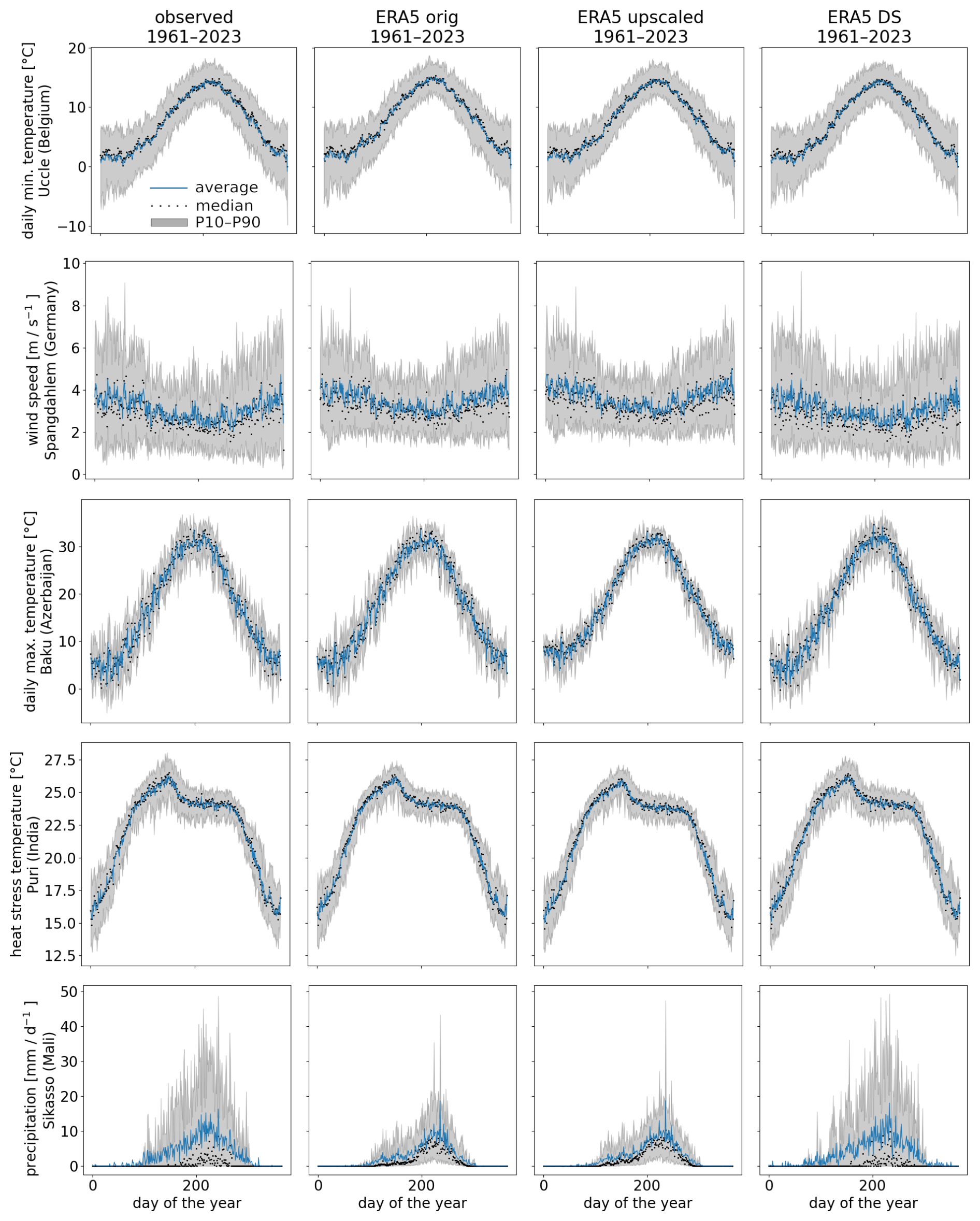
Figure 3 Annual cycles from observations for the period (1961–2023), ERA5 on its original grid (ERA5 orig), ERA5 upscaled to the grid of a climate model (ERA5 upscaled), and ERA5 downscaled with the statistical model (ERA5 DS). The blue lines indicate the average, whereas the black dots show the median of each day of the year over the multiple years. The grey bars indicate the range between the 10th and 90th percentile values over the different years. We show daily minimum temperature for Uccle in Belgium (first row), daily mean wind speed for Dahlem in Germany (second row), daily maximum temperature for Uccle in Belgium (third row), heat stress temperature for Puri in India (fourth row), and precipitation for Sikasso in Mali (last row).

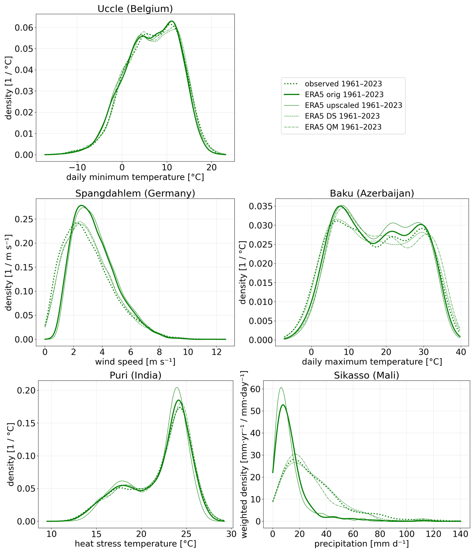
Figure 4 Density distribution from daily observations for the period (1961–2023), ERA5 on its original grid (ERA5 orig), ERA5 upscaled to the grid of a climate model (ERA5 upscaled), and ERA5 downscaled with the statistical model (ERA5 DS). We show daily minimum temperature for Uccle in Belgium (upper panel), daily mean wind speed for Dahlem in Germany (center left panel), daily maximum temperature for Baku in Azerbaijan (center right panel), heat stress temperature for Puri in India (lower left panel), and precipitation for Sikasso in Mali (lower right panel).

Figure 5 Idem as Fig. 4, but for return levels.

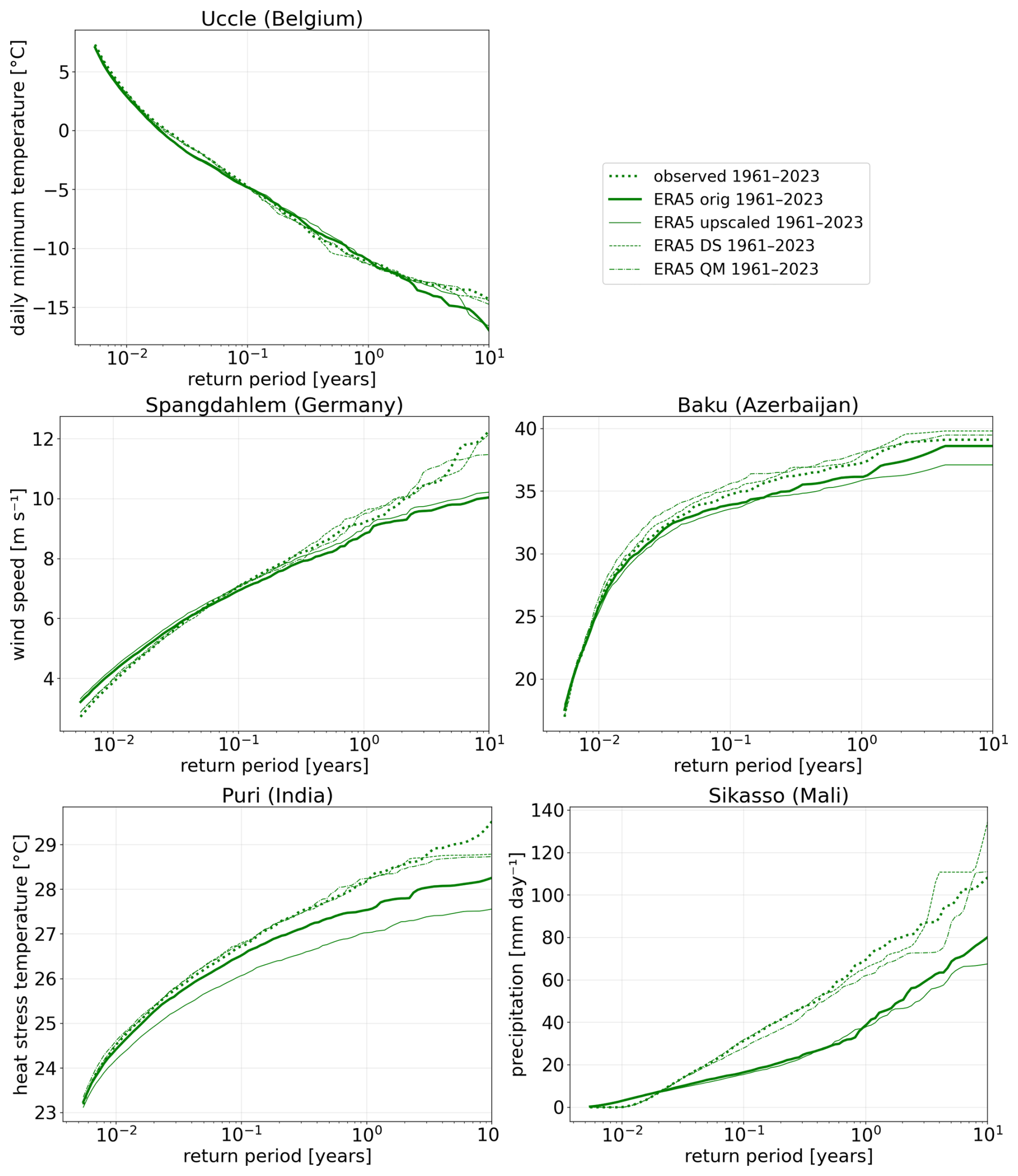
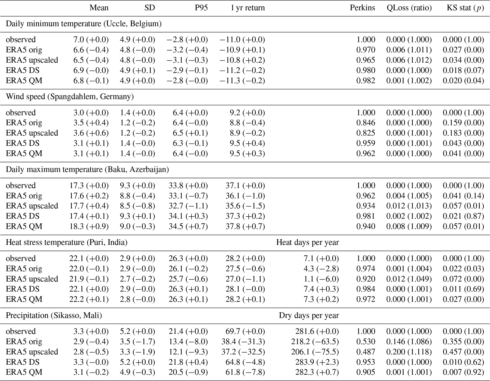
Table 2 Validation metrics for precipitation distributions from observations (Observed), original ERA5 (ERA5 orig), upscaled ERA5 (ERA5 upscaled), fully correlated stochastic downscaling (ERA5 DS), and quantile-mapping-only downscaling (ERA5 QM). For the mean, standard deviation (SD), 95th percentile (P95), 1-year return level (1 yr return), and annual number of dry days (in case of precipitation), absolute values are reported with deviations from observations in brackets. We further report the Perkins overlap score (Eq. 22), the quantile loss difference (with ratio in brackets), and the Kolmogorov–Smirnov statistic with the corresponding p-value.

In contrast, all results for ERA5 downscaled to the station level match better the variability of the annual cycle (Fig. 3) and distribution statistics (Table 2) compared to the original ERA5 and distribution statistics. Herewith, also the overall bias is removed for each variable. The improved representation of extremes by downscaling is also clear from density distributions (Fig. 4) and return periods (Fig. 5). Distributions of precipitation after downscaling are also better matching the observations (thin dashed lines versus thick dashed lines in Fig. 4) than without downscaling of ERA5 (thick line versus thin dashed line), since they get shifted to more high extremes, while also the number of dry days becomes larger and better matching observations (Table 2). At the same time, the downscaling reduces the overall bias in average daily precipitation for Sikasso with a downscaled value of 3.3 mm matching the observed value, whereas it is underestimated by the ERA5 value (2.9 mm). Other variables, particularly daily minimum and maximum temperature, wind speed and heat stress, also show a better match with the observed distribution after downscaling with larger spread (Fig. 4). Besides better statistics on mean and variability, the better match of the distributions after downscaling is confirmed with better score values for Perkins overlap score, the quantile loss difference and the Kolmogorov–Smirnov statistic, see Table 2. All downscaled variables (including daily minimum temperature) show more extreme levels for the high return periods compared to original ERA5 data, for which they approximate the return levels of the observations much better (Fig. 5).

Results and scores with standard quantile mapping (ERA5 QM) are added as comparison next to the full correlated sampling (ERA5 DS), see Figs. 4 and 5, and Table 2. While the results from the standard quantile mapping (ERA5 QM) show similar scores and distributions to the full correlated sampling (ERA5 DS), the latter one is preferred, since the former could lead to inflation of trends in extremes (Maraun, 2013). Inflation for precipitation in Sikasso is also illustrated in Text S2 with the help of Figs. S3, S4 and S5, and Table S3.

3.2 Assessment of extremes under climate change

In this section, assessment is demonstrated for each of the variables for two 30-year timeframes in the past (1961–1990 and 1991–2020) and one in the future under the SSP585 scenario (2071–2100), see Figs. 6, 7 and Table 3.

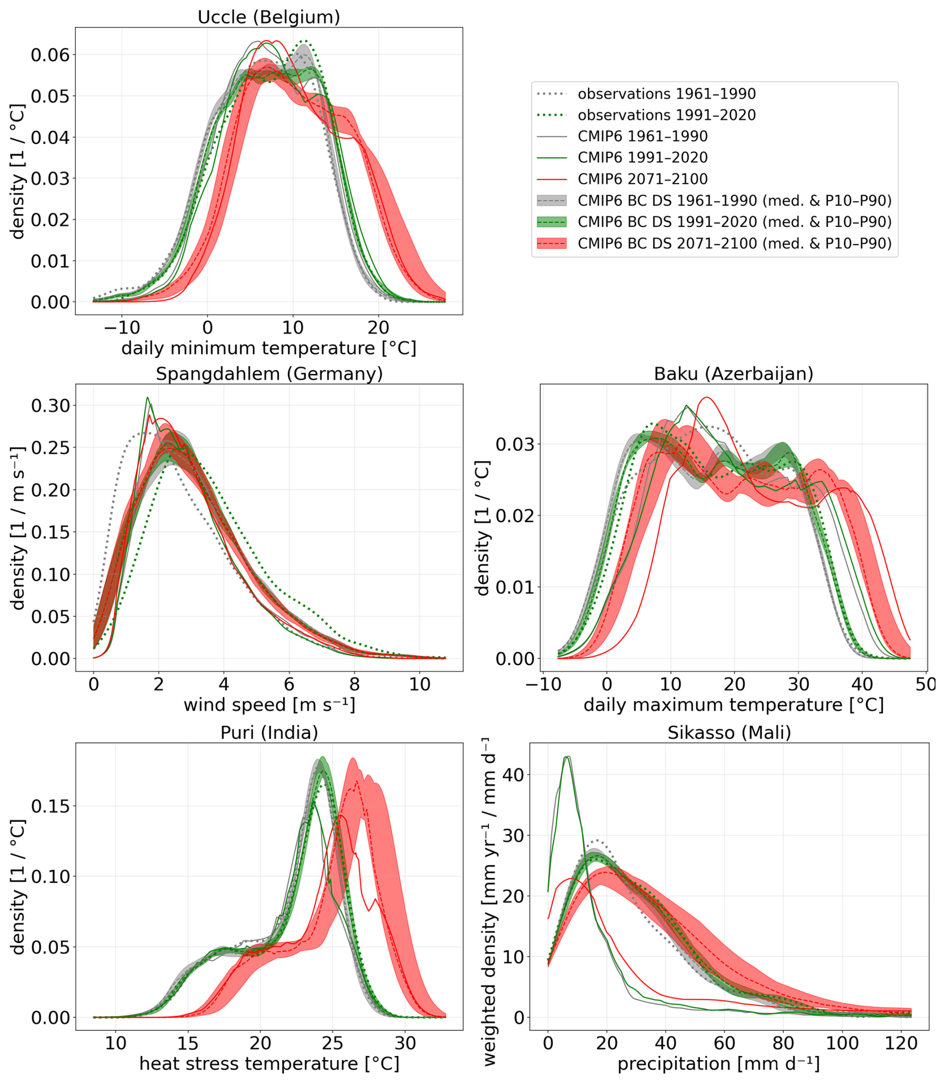
Figure 6 Idem as Fig. 4, but showing results for original CMIP6 climate projections (SSP585) including models listed in Table 1, bias-corrected and downscaled CMIP6 models (CMIP6_BC_DS). Observations are also included as comparison. Results are shown for two historical time frames 1961–1990 (in grey) and 1991–2020 (green), and for one future timeframe 2071–2100 (in red). For CMIP6_BS_DS, we show the 10-to-90 percentile spread over the different models.

Figure 7 Idem as Fig. 6, but for the return levels.

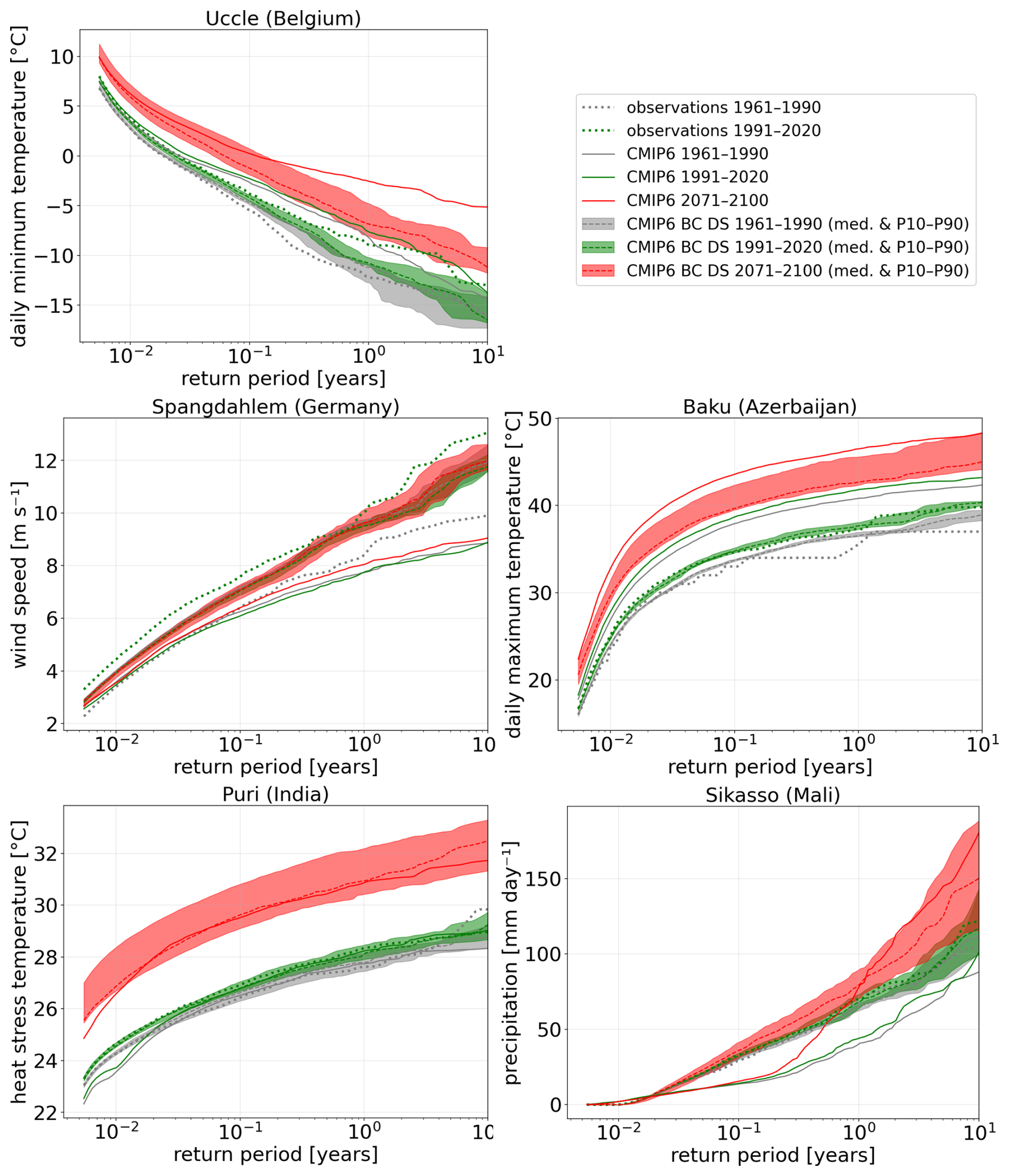
Table 3 Annual mean, standard deviation, percentile 95 value and 1-year return value, annual dry days (for daily precipitation < 1 mm), annual heat days (for heat stress temperature > 27 °C) of observed and modelled time series. We include the original CMIP6 climate projections (SSP585) including models listed in Table 1, and the bias-corrected and downscaled CMIP6 models (CMIP6_BC_DS). Observations are also included as comparison. Results are shown for two historical time frames 1961–1990 and 1991–2020, and for one future timeframe 2071–2100. For the climate projections, we show median and percentile 10–90 ranges of the model ensemble.

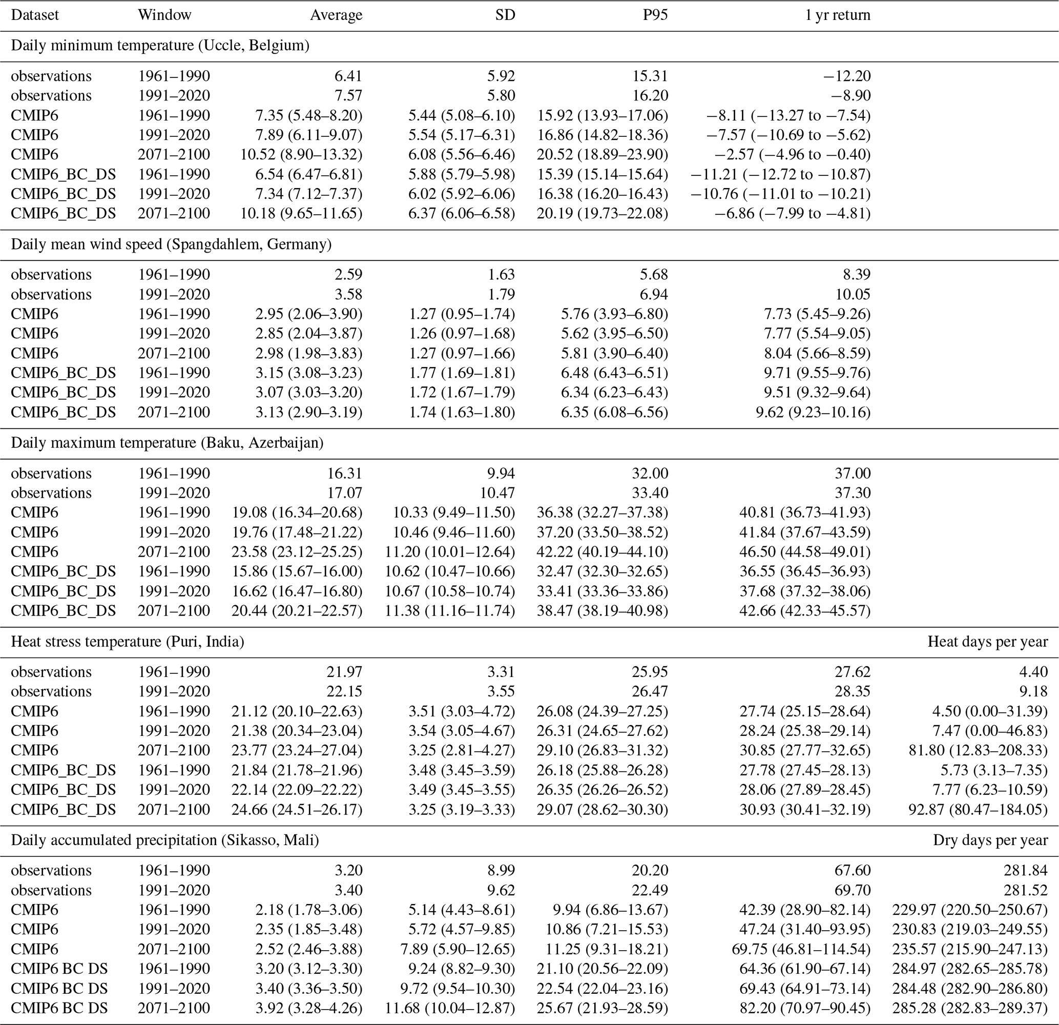
Overall, there is a tendency towards higher (extreme) values for the original climate projections (CMIP6) (see Figs. 6 and 7, and Table 3) under past climate change (thin green line versus thin grey lines). This is except for daily wind speed, for which values remain stable. However, the CMIP6 distributions have substantial biases (thin full lines versus thick dashed lines), just like the ERA5 values as discussed in the previous section. Thanks to the bias-correction and downscaling, the observed distribution (properties) and return levels are now better captured by CMIP6_BC_DS (thin dashed lines versus thick dashed line) for the two past period than for CMIP6 (thin full lines versus thick dashed lines), see Figs. 6 and 7, and Table 3. Hereby, CMIP6_BC_DS alleviates overall biases in the annual averages found for CMIP6 for each variable, see Table 3. Additionally, standard deviations, P95 values, 1-year return levels, and number of dry days (for Sikasso) and heat days (for Puri) generally tend to be higher after downscaling, except for 1-year return values for daily minimum temperature (Belgium) for which we get lower (hence also more extreme) return levels, see Table 3. They lead to a better representation of all these distribution properties, which was also found for ERA5 as shown in the previous section, except for standard deviation for daily maximum temperature (Baku). The past tendencies of standard deviation, P95 and 1-year return values tend to be sligthly lower for CMIP6_BC_DS variables compared to CMIP6. For daily precipitation in Sikasso, this lead to a better representation of the shifts: the tendency of the median 1-year return level between the two 30 year time frames (from 1961–1990 to 1991–2020) is lower for CMIP6_BC_DS (from 65.58 to 67.75 mm) than for the original CMIP6 (from 40.53 to 43.89 mm) which better matches the observed tendency from (from 67.60 to 69.70 mm d⁻¹). The tendency of the P95 value of CMIP6_BC_DS (from 21.02 to 22.22 mm) is still higher than for the original CMIP6 (from 10.97 to 11.20 mm) but that also leads to better match with the observed tendency (from 20.20 to 22.49 mm). For wind speed for Spangdahlem however, the overall distributions of the observations are captured well, but the shift in the observations towards higher wind speeds is not predicted, since large-scale wind speed distribution (CMIP6) doesn't show a shift either.

The tendencies of having higher extremes (except for wind speed) pull through to the end of the 21st century under the SSP585 scenario, see Figs. 6, 7 and Table 3. While original CMIP6 ensemble precipitation already indicates a tendency towards more extremes in the future (red full lines versus green and grey full lines), the tendency of downscaled ensemble (CMIP6_BS_DS) (red dashed lines versus green and grey dashed lines) differs substantially both in absolute and relative numbers. For 1-year return level of daily precipitation, for example, an increase from 40.53 mm (for 1961–1990) to 78.19 mm (for 2071–2100) is found for the median ensemble, hence an increase of 37.6 mm (∼ 76 %), is found for the raw CMIP6. At the same time, an average increase from ∼ 65.58 to ∼ 79.29 mm is found for CMIP6_BS_DS, hence an increase of ∼ 13.7 mm (∼ 20 %). Future temperature, heat stress and wind speed are also affected after downscaling. For heat stress, the (change in) number of days with extreme heat is higher after downscaling (from 5.73 to 92.87 d yr⁻¹) than from the original CMIP6 ensemble median (from 4.50 to 81.80 d yr⁻¹), see Table 3. These results highlight that different types of climate-change assessments using downscaled GCM output lead to different results than those using original GCM output.

4 Conclusions

A downscaling method EXSoDOS is developed for the DOwnscaling of local weather EXtremes Shifts under global warming, including daily minimum and maximum temperature, precipitation, heat stress and wind speed. The model employs ground-based measurements, historical reanalysis climate reconstruction and ensemble climate projections as input. Stochastic modelling is performed by normalizing the local measurements and coarse climate reconstruction and determining the monthly correlation between them for 3 categories of magnitude. Afterwards, the correlation function is applied to different bias-corrected climate model members. The framework uses measurements from the data archive maintained by NOAA (National Oceanic and Atmospheric Administration; https://www.ncei.noaa.gov/pub/data/ (last access: 8 June 2026), the ERA5 reanalysis data from C3S (Copernicus Climate Change Service; https://cds.climate.copernicus.eu, last access: 8 June 2026) and CMIP6 climate projections from ESGF (Earth System Grid Federation; https://metagrid.esgf-west.org/search, last access: 8 June 2026). One can also provide its custom measurement data as alternative observation input, as long as the data has climatological coverage of multiple tens of years.

Each of the extreme weather variables are tested for particular case areas around the world where records are available on climatological time scales. They include daily minimum temperature for Uccle (Belgium), daily maximum temperature for Baku (Azerbaijan), heat stress temperature for Kasungu (Malawi), wind speed for Dahlem (Germany), and daily precipitation in Sikasso (Mali). For these case studies, EXSoDOS was found to reproduce the annual cycle statistics (climatological mean, median and 10th-to-90th percentile range), the density distribution and return periods. The high skill of the model to reproduce extreme occurrences up to 10 year return periods is achieved by the two-step bias-correction and downscaling procedure in line with previous methods (Switanek et al., 2022; Volosciuk et al., 2017).

EXSoDOS was also able to reproduce many of the observed shifts in extreme weather of the past climate (1991–2020 versus 1961–1990), including a tendency to more extreme precipitation and more extreme high temperature and heat stress, and a reduction in cold extremes. While the overall statistics of wind speed were found to be reproduced, the shift in more extreme wind in the observations was not found in CMIP6 or the downscaled time series. Applying the model on future climate projections towards the end of the 21st century (2071–2100), it was found that increasing extremes for daily maximum temperature, precipitation and heat stress are all exacerbated under future global warming. We further show that outcomes of shifting climate extremes are affected in different ways when applying a downscaling. Particularly for precipitation, relative and absolute climate-change signals are affected, as well as the changing return periods. As such, EXSoDOS downscaling is able to offer a baseline estimation of weather extremes and their past and future shifts under global warming for multiple weather variables for the first time, for which the statistical model is constrained with observations at any location on Earth where hyper-climatological (≫ 60 year) measurements are available. Since the algorithm has a low computational cost and uses globally available data, its application could be upscaled to perform assessments for the available data archive of weather stations accross the globe (see Fig. 2), but also for single assessments with available data by local institutes.

The model is only evaluated for 5 sites, hence new applications require additional validation with local data. Nevertheless, the EXSoDOS, including its validation and application, is transferable to any station in the world. We further exemplify transferability by showing results for precipitation for 7 random stations across USA in the supplementary material, see resp. Figs. S1 (validation) and S2 (projection). EXSoDOS should be considered when long-term station weather station data is available and when representation extremes distribution (i.e., tails) at point-scale is important to evaluate past and future climate change. In other cases, one should use existing state-of-the-art archives like CORDEX (Coppola et al., 2021) or CHELSA-W5E5 (Karger et al., 2023) providing grid-scale climate reconstruction and projections down to 1 km resolution.

One should keep in mind the limitations of statistical downscaling when employing the model for future climate assessment. In this manuscript, the model is calibrated and validated with 63 year records, only providing assessments for return periods of up to 10 years. For higher return periods, one requires either substantially longer observational records or an explicit extreme-value extrapolation step requiring additional assumptions (e.g., employing Generalized Pareto Distribution or Generalized Extreme Value Distribution). One should interpret distribution shifts, especially those in far tails, conditional on the uncertainty related to calibration sets and representativeness/stability of correlation between coarse-scale predictor and point-scale predictand under climate change (see sensitivity analysis in Text S1), methodological choices (e.g., detrending/retrending), and the realism of the shifts of the climate predictors at the coarse scale provided by the global climate models.

EXSoDOS also considers only one predictor and one predictand for one location at a time, which implies several limitations. At first, the model doesn't explicitly capture its dependences on multiple local environmental (plant functional types, soil, urban environment…) and climatic parameters (e.g., boundary-layer stability or circulation indicators). As such, the complexity of physical processes may be underrepresented by the model. To perform a more in-depth analysis of changing extremes and their underlying physics, one should still rely on mechanistic high-resolution atmospheric numerical modelling. At second, the simulation of only one output variable (predictand) at a time ignores possible correlation among them, so hampers consistent representation of compound hazards (e.g., heavy drought–heat, heavy rain–wind). At third, modelling one location at a time does not preserve spatial dependence between multiple sites (e.g., a single convective rainstorm affecting multiple sites).

The stochastic model could be improved in several ways. At first, coherent time series for multiple sites and/or multiple variables can be achieved by correlating different predictors and predictands for different variables and different sites. This can by normalizing predictands and predictors, subsequently transforming them to independent variables using their correlation matrix (or Gaussian copula). After such calibration, one combines predictor variables with random sampling and transforms the variables back to the correlated space, and finally one denormalizes them again to their respective distributions. Multi-variable correlated sampling makes representation of compound hazards and spatial dependence between different sites possible. Such a strategy that introduces a correlation matrix over different predictors and predictands is conceptually similar to the multi-site approach proposed by Switanek et al. (2022). At second, extending the predictor set further with environmental and climatic parameters (mentioned above) is a promising avenue to better represent regime-dependent land–atmosphere interactions. Finally to improve the representation of underlying drivers and their shifts under global warming, the correlatied sampling could be upgraded using artificial intelligence, in which one still represents both deterministic predictor–predictand relations and the remaining (unresolved) variability and extremes with stochastic sampling.

Appendix A: Random sampling of a variable correlating with another

We look for α and β in such a way that $\stackrel{\mathrm{̃}}{y}$ correlates with $\stackrel{\mathrm{̃}}{x}$ with correlation coefficient ρ estimated from the calibration above.

$$\begin{array}{}\text{(A1)}& \begin{array}{rcl}\mathit{\rho }& =& \langle \stackrel{\mathrm{̃}}{y}\stackrel{\mathrm{̃}}{x}\rangle \\ & =& \langle \mathit{\alpha }xx\rangle +\langle \mathit{\beta }rx\rangle \\ & =& \mathit{\alpha }{\mathit{\sigma }}_x^{\mathrm{2}}\\ & =& \mathit{\alpha }\end{array}\end{array}$$

where ${\mathit{\sigma }}_{\stackrel{\mathrm{̃}}{x}}=\mathrm{1}$.

$$\begin{array}{}\text{(A2)}& \begin{array}{rcl}{\mathit{\sigma }}_y^{\mathrm{2}}& =& \langle yy\rangle \\ & =& \langle (\mathit{\alpha }x{)}^{\mathrm{2}}\rangle +\langle \mathrm{2}\mathit{\alpha }x\mathit{\beta }r\rangle +\langle (\mathit{\beta }r{)}^{\mathrm{2}}\rangle \\ & =& {\mathit{\alpha }}^{\mathrm{2}}{\mathit{\sigma }}^{\mathrm{2}}+{\mathit{\beta }}^{\mathrm{2}}{\mathit{\sigma }}_r^{\mathrm{2}}\\ & =& {\mathit{\alpha }}^{\mathrm{2}}+{\mathit{\beta }}^{\mathrm{2}}\end{array}\end{array}$$

where ${\mathit{\sigma }}_y={\mathit{\sigma }}_x=\mathrm{1}$. So

$$\begin{array}{}\text{(A3)}& \mathit{\beta }=\sqrt{\mathrm{1}-{\mathit{\alpha }}^{\mathrm{2}}}\end{array}$$