Pre-training for deep statistical climate downscaling: enhancing consistency and robustness across regional datasets

Deep Learning (DL) has recently emerged as a promising approach for statistical climate downscaling. In this study, we investigate the use of pre-training in this context, building on the DeepESD model developed for the Spanish National Adaptation Plan (PNACC), which uses ERA5 predictors and the 5 km ROCIO-IBEB national gridded predictand dataset. We evaluate the effectiveness of different fine-tuning strategies to adapt this pre-trained model to alternative national and regional station (point-based) datasets. The objective is to develop downstream downscaling methods that maintain consistency with the original national-scale model while capturing the specific characteristics of regional and local datasets.

We analyze the benefits of fine-tuning, focusing on the improved consistency and robustness of the resulting models. Using eXplainable Artificial Intelligence (XAI) techniques, we examine the relationships learned by the models and compare the resulting climate change signals. Our results demonstrate that pre-training provides a robust foundation for statistical downscaling, particularly in cases with limited spatial and/or temporal data availability (e.g. local high-resolution datasets available only for short periods), thereby reducing epistemic uncertainty and improving the reliability of future climate projections. Overall, this approach represents a step toward standardizing DL-based downscaling models to ensure more coherent and consistent climate projections across national and regional scales.

1 Introduction

Global Climate Models (GCMs) simulate the spatio-temporal evolution of the climate by numerically solving the physical set of equations that govern its dynamics (Chen et al., 2021). GCMs are used to generate future projections along different forcing or greenhouse gas emission scenarios, providing possible future socio-economic pathways (Eyring et al., 2016). However, due to inherent physical and computational limitations, the resulting projections have a coarse spatial resolution, which limits their suitability for regional studies. Statistical downscaling (Maraun and Widmann, 2018) addresses this limitation by employing statistical models to learn the relationship between coarse large-scale variables (predictors) and the local variable (predictand) of interest (Gutiérrez et al., 2019).

Recently, Deep Learning (DL) (Goodfellow et al., 2016; Prince, 2023) has emerged as a powerful tool for statistical downscaling, thanks to its ability to model non-linear relationships and effectively process spatial data. As a result, DL techniques have been applied to a wide range of statistical downscaling problems, from simple super-resolution (Vandal et al., 2017; Sha et al., 2020a, b) and bias adjustment (François et al., 2021) methods, to more sophisticated Perfect Prognosis (PP) (Baño-Medina et al., 2020, 2022) and emulation (Doury et al., 2023, 2024; Baño-Medina et al., 2023) approaches which rely on large-scale synoptic predictors – reliably simulated by GCMs – to learn empirical relationships with regional or local variables of interest.

Deep PP downscaling methods (hereafter deep downscaling) have already been used to produce regional climate change projections in various regions (Baño-Medina et al., 2021, 2022; Soares et al., 2023; Balmaceda-Huarte et al., 2024). For example, the new generation of regional climate change scenarios for the Spanish National Adaptation Plan, based on CMIP6 (Escenarios-PNACC 2024), includes a deep learning downscaling method (DeepESD) developed using ERA5 predictors and a 5 km gridded observational dataset over Spain (González-Abad and Gutiérrez, 2025). These downscaled scenarios serve as the primary source of information for developing impact assessments and adaptation studies in Spain. However, other regional scenario datasets have also been produced for specific applications or sub-regions, using alternative high-resolution grids or point-based station data with different downscaling techniques (Monjo et al., 2016; Amblar-Francés et al., 2020; Miró et al., 2021; Hernanz et al., 2022). Such methodological diversity, arising from limitations in the techniques used to construct these datasets or from restricted temporal or spatial coverage, can lead to divergent outcomes that may confuse end users. The possibility of using a baseline downscaling model that can be adapted to new target datasets (e.g. higher-resolution gridded products, station/point observations, or alternative data sources) would improve the overall consistency of model outputs while facilitating the generation of downstream scenario products. In addition, having a model with pre-learned relationships could be especially valuable in low-data regimes, which are common when working on specific regional scenarios where the amount of available data is often limited.

One promising approach to achieve this is to rely on pre-training (Bengio et al., 2006; Vincent et al., 2010; Erhan et al., 2010). In this paradigm, a DL model is first pre-trained on one or more source datasets and then fine-tuned on one or several target datasets. Pre-training and fine-tuning have been successfully applied in a wide range of domains, most commonly to improve performance on downstream tasks. For instance, much of the recent success of large language models can be attributed to extensive pre-training on massive amounts of data (Radford, 2018; Devlin et al., 2019; Brown, 2020), followed by task-specific fine-tuning. Similarly, in computer vision, pre-training has enabled models to learn rich spatial representations that transfer effectively across tasks (Dosovitskiy, 2020; Radford et al., 2021; Caron et al., 2021; He et al., 2022). More recently, in weather and climate science, large deep models have been trained on diverse datasets to capture a broad range of physical phenomena (Nguyen et al., 2023; Lessig et al., 2023; Bodnar et al., 2025; Schmude et al., 2024).

In this study, we investigate pre-training for deep statistical downscaling with a different objective. Rather than focusing primarily on maximizing predictive skill for a given dataset, we use pre-training to encourage the learning of general-purpose representations that can serve as a stable common baseline across heterogeneous datasets, thereby improving cross-dataset consistency and robustness to dataset shifts in the resulting model outputs. During pre-training, the model learns broad, transferable structures that can later be adapted through fine-tuning to accommodate dataset-specific characteristics without substantially altering the underlying relationships.

We build on the DeepESD convolutional model originally developed for the Spanish National Adaptation Plan (PNACC), which downscales coarse-resolution GCM predictors to a high-resolution (5 km) national gridded observational dataset (González-Abad and Gutiérrez, 2025). Using this pre-trained model as a baseline, we explore the effectiveness of various fine-tuning strategies to adapt it for alternative national or higher-resolution regional predictand datasets. Rather than seeking to maximize predictive skill for each individual dataset, the objective is to develop cost-effective downscaling approaches that preserve coherence with the national-scale results while accommodating the specific characteristics of local datasets. This is particularly relevant for the generation of national and regional climate change scenarios based on multiple observational products, as illustrated here for the regional scenarios produced within the PNACC framework. In such applications, maintaining coherent climate-change signals across products is essential for downstream impact assessments and decision-making.

We focus on daily minimum and maximum temperature and precipitation. To test the fine-tuning strategies, we employ two alternative point-based observational datasets: one national and one regional. The national dataset comprises more than 3400 stations for temperature and 5800 stations for precipitation across peninsular Spain. In contrast, the regional dataset covers the region of Catalonia and includes 114 temperature and 110 precipitation stations over a shorter temporal period, thereby reflecting the types of data limitations that the proposed methodology is designed to address. These station-based datasets constitute a compelling test case due to their distinct spatial resolution and observational nature relative to the original gridded data.

To assess the consistency and interpretability of the fine-tuned models, we analyze the learned relationships using eXplainable Artificial Intelligence (XAI) techniques (Adadi and Berrada, 2018; Arrieta et al., 2020; Minh et al., 2022). Beyond quantifying which predictors a model relies on, in this work we also emphasize whether the learned relationships aligns with the synoptic processes that drive relevant local events (such as extreme precipitation), for which there is a physically motivated expectation of where a skillful model should attend. This alignment provides a more demanding test of the trustworthiness and transferability of the learned relationships since a model can achieve competitive metrics while relying on spurious relationships that are especially problematic under the extrapolation to future climate (González-Abad et al., 2023). In this sense, our analysis pushes saliency-based XAI beyond diagnostic sensitivity analysis toward a physically interpretable evaluation of the learned relationships, motivating the case-wise saliency analyses presented in this work.

The paper is structured as follows. Section 2 introduces the data, the DL model, and the XAI techniques used in this work. In Sect. 3, we present the pre-training and fine-tuning strategies in detail. Section 4 provides the results of all the experiments conducted in this study. Finally, in Sects. 5 and 6, we discuss these results and conclude with the main findings of this work.

2 Experimental framework

In this section, we first describe the region of study, the datasets, and the preprocessing procedures. We then provide a detailed overview of DeepESD, the deep downscaling architecture that serves as the foundation for this work. Finally, we introduce the techniques used to assess the deep downscaling models, focusing on the relationships they learn.

2.1 Region of study

We focus on peninsular Spain (36–44° N, 9.5° W–3.5° E), which represents a challenging benchmark for statistical downscaling due to its diverse climatology and complex orography. This region, located within the Mediterranean basin, is significantly affected by climate change, experiencing increasing temperatures and changes in precipitation patterns (Hoerling et al., 2012; Cos et al., 2022).

In this region, multiple observational datasets are available, including several gridded datasets such as ROCIO-IBEB (5 km resolution Peral García et al., 2017), Iberia01 (10 km resolution Herrera et al., 2019) and E-OBS (10 km resolution Cornes et al., 2018), as well as higher-resolution grids over specific sub-domains (Basque Government, 2020; Taboada et al., 2024). This provides opportunities to extend this work using multiple datasets of different natures for pre-training and/or fine-tuning.

2.1.1 Predictor and predictands

As predictors, we select a set of large-scale atmospheric variables commonly used in previous climate downscaling studies (Gutiérrez et al., 2013; Baño-Medina et al., 2021; Soares et al., 2023), specifically air temperature, specific humidity, and meridional and zonal wind velocity at 850, 700, and 500 hPa and mean sea level pressure. These predictors are obtained from the ERA5 reanalysis dataset (Hersbach et al., 2020) and regridded from their original 0.25° resolution to 1.5° using conservative interpolation, to match the coarser scales typical of GCM outputs.

To ensure that large-scale phenomena influencing the downscaled variables are fully captured, we extend the spatial domain to 23.5–68.5° N and 39° W–22.5° E. Finally, to avoid biases from differing variable scales, each predictor grid point is standardized to a zero mean and unit variance before being fed into the model.

For this study, we used three types of observational data from the Spanish Meteorological Agency (AEMET) and the European Climate Assessment & Dataset (ECA&D) as predictands: the ROCIO-IBEB gridded dataset (Peral García et al., 2017), which provides daily precipitation and temperature at 5 km resolution; station observations from the STATIONS-IBEB network (Spanish Meteorological Agency, 2021), comprising over 5800 precipitation and 3400 temperature ground stations; and the STATIONS-CAT dataset, which denotes a specific subset of the ECA&D blended daily series (Klein Tank et al., 2002; Klok and Klein Tank, 2009), consisting of 110 precipitation and 114 temperature stations across Catalonia. ROCIO-IBEB served as the predictand for developing the deep downscaling model used to generate high-resolution gridded projections under the Spanish National Adaptation Plan (PNACC). In this study, we pre-train the downscaling model on ROCIO-IBEB and then fine-tune it on both STATIONS-IBEB and STATIONS-CAT observations. Notably, STATIONS-CAT provides an independent validation of our fine-tuning approach, as these stations were not used in the construction of ROCIO-IBEB, unlike STATIONS-IBEB. We also train separate models from scratch using STATIONS-IBEB and STATIONS-CAT as predictands to benchmark the benefits of the fine-tuning approach. We refer to these models as fully-trained to indicate that they are trained entirely on their respective station datasets, without leveraging any pre-trained model on ROCIO-IBEB.

Figure 1 presents both the climatologies of mean and extreme-related indices for each of the three predictands (minimum temperature, maximum temperature and precipitation) for all datasets. Specifically, we show the mean values of the three variables as well as the annual minimum of daily minimum temperatures (TNn), the annual maximum of daily maximum temperatures (TXx), and the annual maximum daily precipitation (RX1day). Regional differences driven by orography and coastal vs. inland conditions are apparent in all datasets. Although the ROCIO-IBEB gridded product is derived from STATIONS-IBEB observations, the station-based dataset shows some differences in extreme values, especially for precipitation. The STATIONS-CAT dataset, despite being independent of the other two, shows similar trends and values, more aligned with those of STATIONS-IBEB. It is also worth noting that for STATIONS-IBEB the number of available stations for precipitation is higher, as reflected in the denser precipitation maps. For STATIONS-CAT, the number of stations is considerably lower than STATIONS-IBEB but similar between variables.

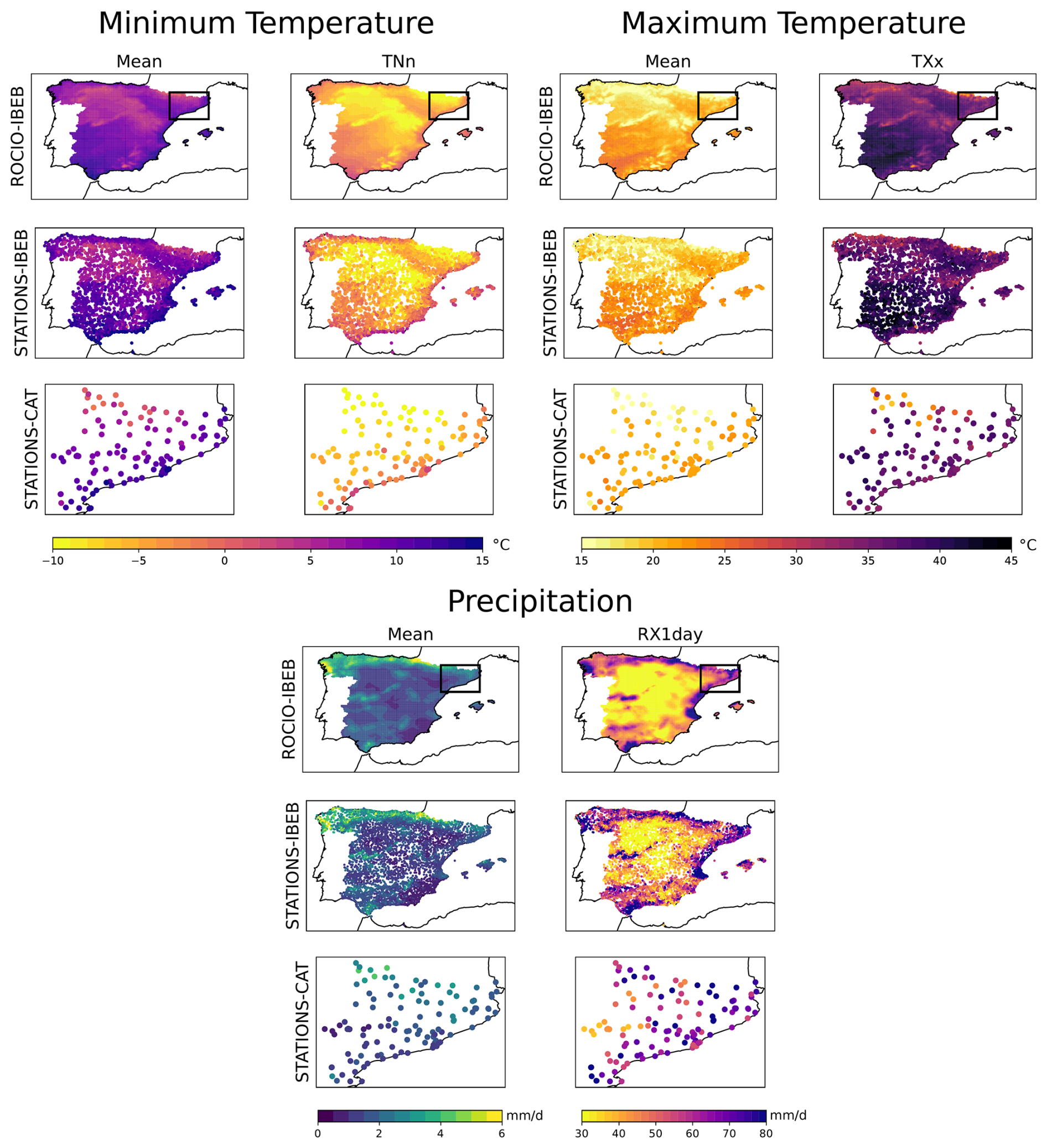
Figure 1 Climatologies of minimum and maximum temperatures and accumulated precipitation. For each of the three variables, we show both the mean climatology and an extreme-related statistic: the annual minimum of daily minimum temperatures (TNn), the annual maximum of daily maximum temperatures (TXx), and the annual maximum daily precipitation (RX1day). Each variable's climatology is computed for the ROCIO-IBEB, STATIONS-IBEB and STATIONS-CAT datasets (arranged in rows within each subpanel). For the ROCIO-IBEB and STATIONS-IBEB datasets, climatologies are computed over the period 1980–2010, while for STATIONS-CAT they are computed over 2009–2018. The spatial extent of the STATIONS-CAT dataset is indicated in the ROCIO-IBEB panels.

2.1.2 Historical and future projections

To evaluate the performance of the DL model to downscale future projections from GCMs, we follow previous studies (González-Abad and Gutiérrez, 2025) and use the EC-Earth3-Veg climate model (Döscher et al., 2021), which is among the GCMs recommended by EURO-CORDEX for downscaling CMIP6 over the European domain (Sobolowski et al., 2023), also used in Escenarios-PNACC (Correa et al., 2023). We use predictor data from the historical (1980–2014) and a future scenario (SSP3-7.0, 2071–2100) representing high emission forcing conditions. Following the assumptions of the PP approach and previous studies (Baño-Medina et al., 2021, 2022; Addison et al., 2024), we apply a simple mean-variance bias adjustment to the GCM predictors to ensure that their distribution more closely matches that of their ERA5 reanalysis counterparts. For further details on this transformation, we refer the reader to Baño-Medina et al. (2021). Prior to feeding the bias-adjusted GCM outputs into the deep-learning model, we standardize them using the ERA5 grid-box means and variances.

2.2 Deep learning model

We select the DeepESD architecture (Baño-Medina et al., 2022) as the basis for the standard DL model. This choice is motivated by several factors. First, while not representing the current state-of-the-art in ML-based downscaling, this model is among the most widely adopted for generating climate projections from GCMs, having been applied to various regions, including continental Europe (Baño-Medina et al., 2020, 2021), southern South America (Balmaceda-Huarte et al., 2024), Egypt (Kheir et al., 2023), New Zealand (Rampal et al., 2022), Germany (Quesada-Chacón et al., 2022), and, more recently, Iberia (Soares et al., 2023; González-Abad and Gutiérrez, 2025). Second, this model has been explicitly assessed for its plausibility in future climate scenarios (Baño-Medina et al., 2021; González-Abad and Gutiérrez, 2025), an aspect that is often overlooked in downscaling studies (Rampal et al., 2024). Third, its promising results are achieved without having to rely on a complex or highly specialized architecture, making it particularly suitable for the approach explored in this study.

The DeepESD architecture employed in this work consists of three successive convolutional layers with 50, 25, and 1 kernels, respectively, each followed by a Rectified Linear Unit (ReLU) activation function (Glorot and Bengio, 2010) (see Fig. 2 for a schematic overview). In the original design (Baño-Medina et al., 2020), the last convolutional layer for temperature was formed by 10 kernels instead of one. However, using 10 kernels substantially increases the network's complexity, raising the parameter count, for instance in the case of ROCIO-IBEB, from approximately 28 million (with a single final kernel) to 284 million. This increase arises from the final dense layer, which fully connects the output of the last convolutional kernel to every grid point to be downscaled. Such an overparameterized DL model may be prone to overfitting (Bishop and Nasrabadi, 2006; Hastie et al., 2001), potentially learning spurious relationships that fail to extrapolate in future scenarios, as discussed in González-Abad et al. (2023). Consequently, we choose to employ the DeepESD architecture with a single kernel in the final convolutional layer for all three variables. The output of this layer is then flattened and passed to a final dense layer, which has as many neurons as the number of points to be downscaled, 21 885 for ROCIO-IBEB, 3460 (5803) for temperature (precipitation) for STATIONS-IBEB and 114 (110) for temperature (precipitation) for STATIONS-CAT. The differences in STATIONS-IBEB originate from the greater number of stations available for precipitation (see Sect. 2.1).

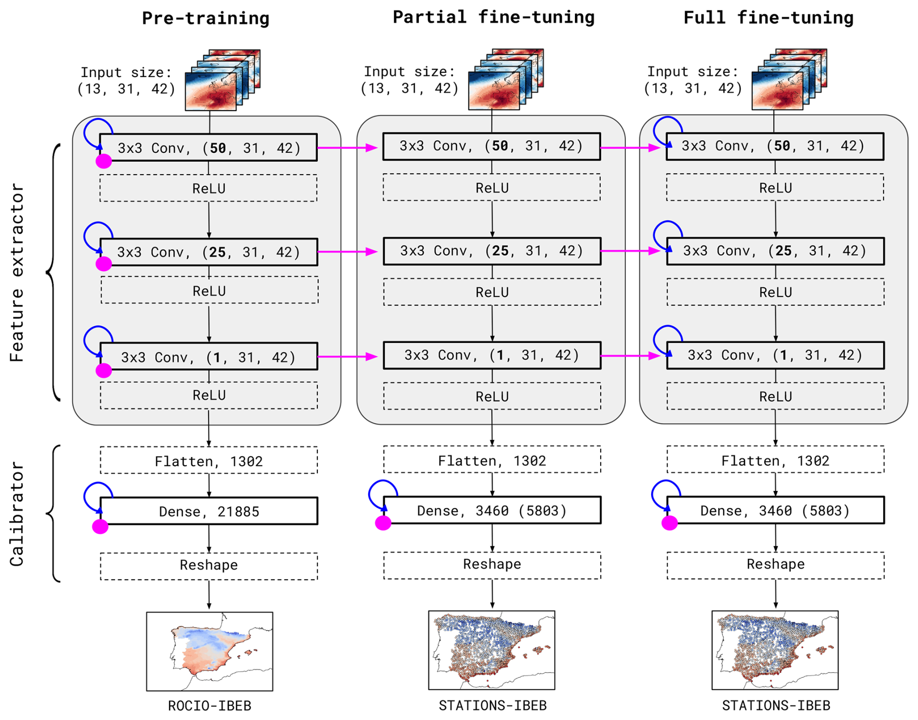
Figure 2 Schematic representation of the three training regimes: pre-training (left), partial fine-tuning (center), and full fine-tuning (right). Each model is composed of convolutional and dense layers, grouped into two main blocks: the feature extractor (gray box) and the calibrator. Initialization is represented in purple, with points indicating random weights and arrows indicating initialization from pre-trained models. Blue looping arrows represent training. Layers with learnable parameters are shown with solid borders, while non-trainable layers are indicated with dashed borders. The schematic illustrates the configuration for the ROCIO-IBEB dataset. The same procedure applies to STATIONS-CAT, differing only in the number of stations represented in the final dense layer.

All DL models for the three variables are trained using the same procedure. We employ the Adam optimizer (Kingma, 2014) with a learning rate of 10⁻⁴ and a batch size of 64 to minimize the loss function. For temperature, we use the Mean Squared Error (MSE), a widely adopted loss function in temperature downscaling. In contrast, selecting an appropriate loss function for precipitation is less straightforward due to its non-continuous and exponentially distributed nature. A recent study (González-Abad and Gutiérrez, 2025) found that the asymmetric (ASYM) loss function proposed in Doury et al. (2024) is well-suited for precipitation downscaling. Consequently, we use the ASYM loss function for precipitation.

To account for variability in training performance, each model is trained ten times per variable using different random initializations of its weights. To properly evaluate the DL models, we split the dataset into training (1980–2010 for STATIONS-IBEB and 2009–2018 for STATIONS-CAT) and test sets (2011–2020 for STATIONS-IBEB and 2019–2021 for STATIONS-CAT). Additionally, during training, we set aside 10 % of the training data as a validation set. This validation set is used to implement an early stopping strategy with a patience of 60 epochs, ultimately selecting the model that performs best on the validation set during this period.

2.3 Explainable artificial intelligence

A key factor underlying the success of DL models is their internal structure, which involves the composition of multiple piecewise/non-linear functions and a large number of parameters. However, this complexity also makes these models difficult to interpret, often branding them as black-boxes, as the relationships they learn are not readily apparent. This issue is particularly relevant in statistical downscaling, where the field has transitioned from simple, interpretable models to complex, deep neural networks. To address this challenge, eXplainable Artificial Intelligence (XAI) techniques have emerged, offering insights into the inner workings of DL models and shedding light on the relationships they capture (Adadi and Berrada, 2018; Arrieta et al., 2020; Minh et al., 2022). Within the statistical downscaling domain, the application and benefits of XAI have only recently begun to be explored (Baño-Medina, 2021; Rampal et al., 2022; González-Abad et al., 2023; Baño-Medina et al., 2023; Balmaceda-Huarte et al., 2024).

In this study, we explore the relationships learned by the different DL models trained in the different regimes by applying the XAI-based diagnostics introduced in González-Abad et al. (2023), specifically designed for the context of PP downscaling. These diagnostics are based on saliency maps, which quantify the sensitivity of the model outputs to variations in the input predictors by measuring the gradient of the predictand with respect to the predictor. In this work, saliency maps are exploited in three complementary ways. First, they are analyzed directly by aggregating them over time, providing an average spatial representation of the saliency distribution relative to a single predictand grid point. Second, we compute the Aggregated Saliency Map (ASM), a diagnostic that summarizes the overall spatial influence of each predictor variable by aggregating saliency values across both time and all predictand grid points. This enables identification of the predictors that exert the strongest influence on the model outputs. Third, saliency maps are computed for individual days corresponding to extreme precipitation events at a given predictand grid point, enabling a case-wise comparison of the saliency patterns learned by the DL models.

In this work, we compute the required saliency maps by directly calculating the gradients of the predictand space with respect to the predictor space. We then apply the same preprocessing steps to these saliency maps as in González-Abad et al. (2023) before computing the final diagnostics.

3 Pre-training and fine-tuning

Figure 2 presents a schematic view of the pre-training (left), partial fine-tuning (center), and full fine-tuning (right) regimes. For each regime, the corresponding DeepESD architecture is shown, with layers represented by small boxes indicating the number of neurons and kernel dimensions for the convolutional layers. The DeepESD architecture, across all training regimes, is divided into two distinct components: the feature extractor (depicted by the gray box in Fig. 2) and the calibrator. The feature extractor, composed of convolutional layers, is responsible for learning high-level data representations. The calibrator, consisting of a dense layer, transforms these high-level features into localized predictions at each grid point of the predictand, enabling the model to perform point-by-point downscaling. Importantly, the architecture remains consistent across all three downscaled fields due to the design choice regarding the number of kernels in the final convolutional layer, as discussed in Sect. 2.2.

First, the DeepESD model is trained using ERA5 as the predictor and ROCIO-IBEB as the predictand, resulting in the pre-trained model shown in Fig. 2. In this model, weights are randomly initialized, as indicated by the purple dots, and trained, as indicated by the blue arrows looping back to each layer. This corresponds to the standard training procedure for DL models. The pre-trained model then serves as the foundation for two additional variants: the partial fine-tuned and the full fine-tuned models. Both of these variants are trained using STATIONS-IBEB or STATIONS-CAT as the predictand, but the weights of their feature extractors are initialized using the weights learned by the pre-trained model, as shown by the purple arrows connecting the feature extractor layers across models. In the partially fine-tuned model, the feature extractor layers are frozen (i.e. not updated during training), and only the calibrator is trained, which is reflected by the absence of blue arrows for the feature extractor and its presence for the calibrator. In contrast, the fully fine-tuned model also allows the feature extractor layers to fine-tune the weights inherited from the original trained model during training.

The decision to transfer only the feature extractor originates from the role that convolutional layers play in learning high-level data representations that are often transferable across related tasks (LeCun and Bengio, 1995; Krizhevsky et al., 2012; Agrawal et al., 2014). This is particularly relevant for the DeepESD model, where the convolutional layers capture high-level synoptic patterns, while the final dense layer provides spatial specialization by fitting a linear regression over these representations for each grid point forming the predictand (Baño-Medina, 2021; González-Abad et al., 2023).

Although the feature extractor contains a relatively small fraction of the total model parameters, parameter count alone does not reflect functional importance (Goodfellow et al., 2016). The calibrator's large parameter count arises from its scaling with the number of output locations, but functionally it performs location-dependent linear mappings from the learned representations. In contrast, the feature extractor learns the nonlinear representations that determine what information is available to the final layer. In addition, prior work shows that transferability depends strongly on layer role/depth, with earlier representation layers often being more transferable than later task-specific layers (Yosinski et al., 2014).

Transferring only the weights of the convolutional layers (i.e. the feature extractor) aligns with standard practices in other domains, such as computer vision and natural language processing, where fine-tuning typically involves appending a task-specific layer to a trained backbone (or to the encoder in encoder-decoder architectures) (Devlin et al., 2019; Chen et al., 2020). The comparison between freezing these transferred weights and fine-tuning them reflects two prevalent strategies in the pre-training literature, where some studies keep the transferred layers fixed, while others allow them to adapt during training.

4 Results

In this section, we examine the feasibility of a pre-training strategy by comparing the performance and key characteristics of models originally trained on ROCIO-IBEB and fine-tuned on STATIONS-IBEB with those of a model fully trained from scratch on STATIONS-IBEB using randomly initialized weights. Throughout the manuscript, we refer to this latter approach as full-training. Additionally, we present a case study using the STATIONS-CAT dataset (a regional dataset independent of ROCIO-IBEB) to demonstrate how fine-tuning enhances the robustness of climate change signals and produces more aligned and physically consistent learned relationships compared to training from scratch.

4.1 Performance of deep downscaling models

In Fig. 3, we present the evaluation results on the test set for the four DeepESD models: the model pre-trained on ROCIO-IBEB (pre-training), the model exclusively trained on STATIONS-IBEB (full-training), and the two models fine-tuned on STATIONS-IBEB using as foundation the pre-trained model (partial and full fine-tuning). Results are shown for minimum (top) and maximum (bottom) temperature. For both variables, we report the Root Mean Square Error (RMSE) and the bias of the mean. Additionally, we include the bias in the annual minimum of daily minima (TNn) for minimum temperature, and the bias in the annual maximum of daily maxima (TXx) for maximum temperature. Note that the violin plots correspond to a randomly selected training run. To illustrate variability across model initializations, we include black dashed lines showing the minimum and maximum values of the spatial medians across the ten training replicas.

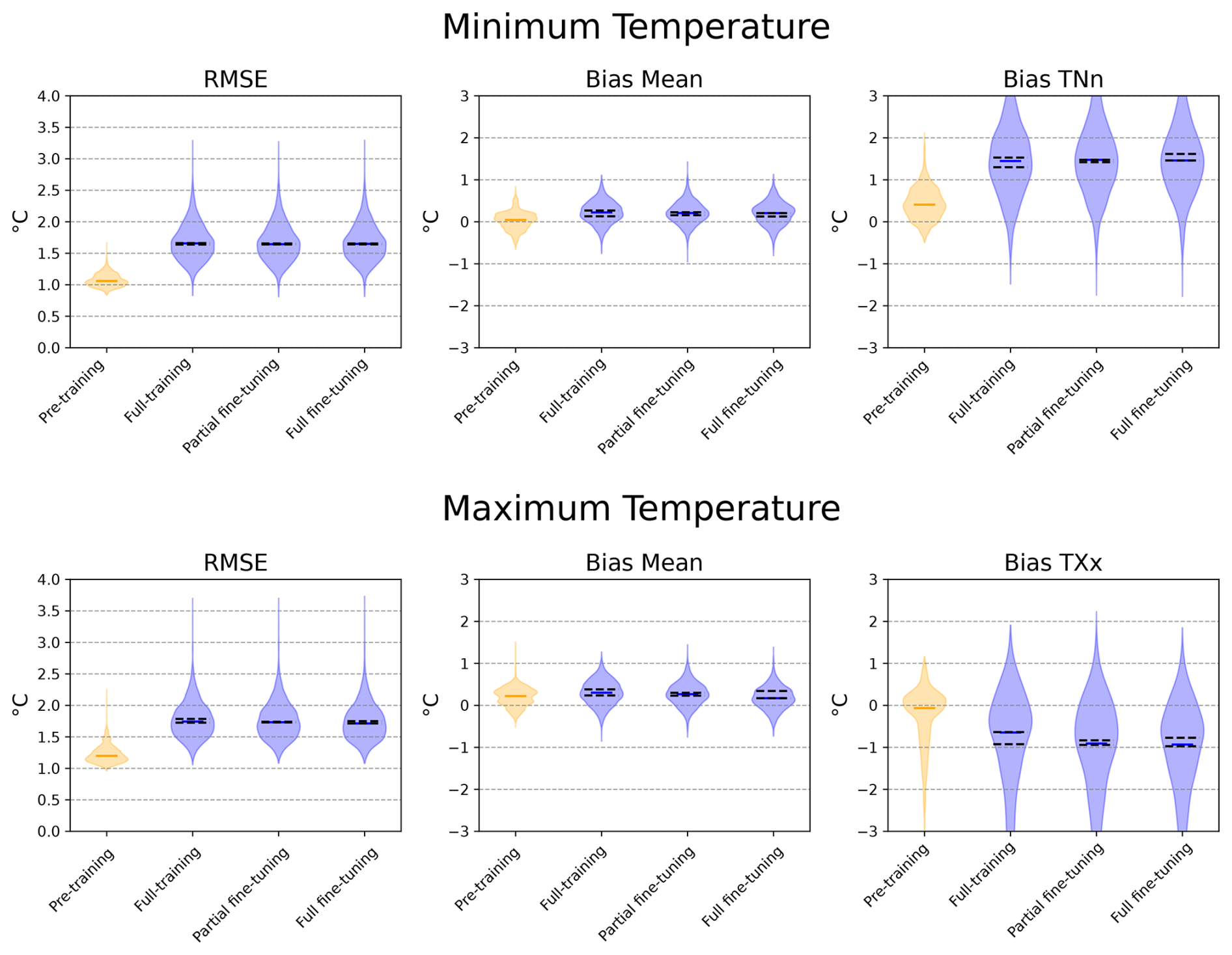
Figure 3 Evaluation results on the test set (2011–2020) for the DeepESD model trained under the different regimes: pre-training on ROCIO-IBEB, and full-training, partial fine-tuning and full fine-tuning on STATIONS-IBEB. Results are shown for minimum temperature (top row) and maximum temperature (bottom row). For both variables, we report the Root Mean Square Error (RMSE) and the bias of the mean (Bias Mean). Additionally, for minimum temperature, we include the bias in the annual minimum of daily minima (TNn), and for maximum temperature, the bias in the annual maximum of daily maxima (TXx). Violin plots show the distribution across grid points for a given training run (randomly chosen), with the spatial median marked in blue. Black dashed lines indicate the range of spatial medians across the ten independent training runs.

The pre-trained model results on ROCIO-IBEB, consistent with previous studies (Soares et al., 2023; González-Abad and Gutiérrez, 2025), are shown for reference to illustrate the characteristics of this gridded dataset. However, these results are not directly comparable to the STATIONS-IBEB models, as they involve different predictand datasets with distinct spatial characteristics. Among the three models trained on STATIONS-IBEB (full-training, partial fine-tuning and full fine-tuning), performance is similar across metrics, though overall accuracy is lower than for the ROCIO-IBEB model due to the more challenging nature of station-based datasets. Notably, the partially fine-tuned model displays slightly lower variability in the spatial median, particularly for the bias in extremes (TNn and TXx), suggesting improved robustness across training runs.

Figure 4 presents the equivalent analysis for precipitation. We show the Root Mean Square Error (RMSE) computed over wet days ($>\mathrm{1}\mathrm{mm}{\mathrm{d}}^{-\mathrm{1}}$), the bias in the frequency of dry days, the Simple Daily Intensity Index (SDII), and the bias in the annual maximum daily precipitation (Rx1day). As noted for temperature, the pre-trained model results on ROCIO-IBEB serve as a reference and align with previous studies, but are not directly comparable to the STATIONS-IBEB models. Among the three STATIONS-IBEB models, results are comparable overall, though for the bias of the SDII, the partially fine-tuned model performs slightly worse than the fully-trained and fully fine-tuned versions.

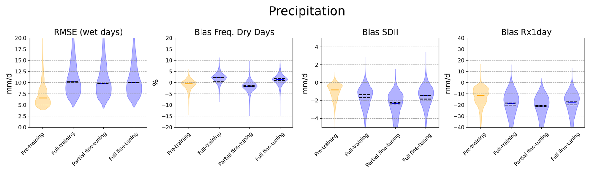
Figure 4 Same evaluation as in Fig. 3 but for precipitation. Metrics include the Root Mean Square Error (RMSE) computed over wet days ($>\mathrm{1}\mathrm{mm}{\mathrm{d}}^{-\mathrm{1}}$), the bias in the frequency of dry days (Bias Freq. Dry Days), the bias in the Simple Daily Intensity Index (Bias SDII), and the bias in the annual maximum daily precipitation (Bias Rx1day).

4.2 Explainability: saliency of the different predictors

To analyze the relationships learned by the deep downscaling models, we use the XAI-based ASM diagnostic based on aggregated saliency (see Sect. 2.3 for details). Figure 5 displays this diagnostic computed over the test set for all predictor variables for the three downscaled variables (shown in separate subplots) and for the pre-trained on ROCIO-IBEB and fully-trained, partially fine-tuned and fully fine-tuned models on STATIONS-IBEB. In previous work (González-Abad et al., 2023), ASM values are depicted for every grid point in each predictor variable, thereby illustrating spatial patterns of relevance. However, to simplify our analysis, we aggregate the ASM spatially, showing a single value per predictor variable that represents its overall importance for the deep downscaling model. In Fig. 5, these aggregated saliency values are displayed as histograms, with the color of each bar (gray, red, green, or blue) corresponding to the different models.

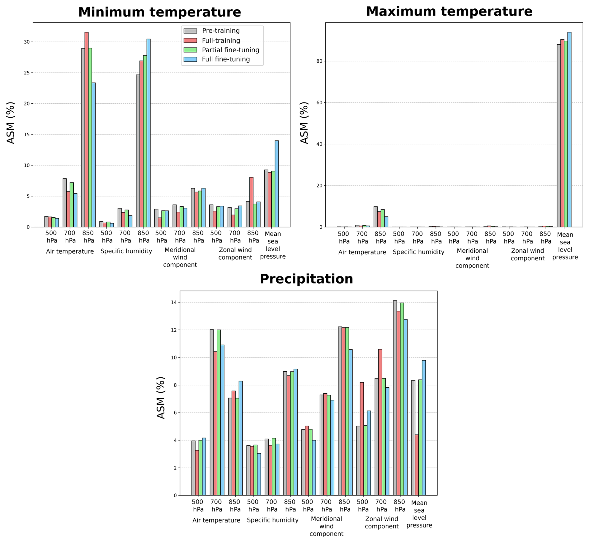
Figure 5 Aggregated Saliency Map (ASM) computed over the test set for the three downscaled variables (shown in separate subplots). The model pre-trained on the ROCIO-IBEB dataset is depicted in gray, while the three models for STATIONS-IBEB (full-training, partial fine-tuning and full fine-tuning) are shown in red, green, and blue, respectively. The ASM is spatially aggregated for each predictor variable, resulting in a single importance value per variable, as represented by the bars.

For minimum temperature, the ASM for both the pre-trained and the three STATIONS-IBEB models is distributed across multiple variables, with air temperature and specific humidity at 850 hPa, along with mean sea level pressure, emerging as the most relevant. However, the model trained on the ROCIO-IBEB dataset (pre-training) and the STATIONS-IBEB trained model (full-training) differ in how they attribute importance to certain variables (for example, the zonal wind component at 850 hPa). This discrepancy diminishes when the weights of the feature extractor are transferred (fine-tuning), resulting in a closer alignment with the pre-trained model. Interestingly, the full fine-tuning diverges more noticeably in its ASM, showing greater differences in variable relevance than even the fully-trained model for some predictors (e.g. mean sea level pressure). For maximum temperature, the pattern is notably different. In both the pre-trained model and the three STATIONS-IBEB models, nearly all relevance is assigned to mean sea level pressure, with only a minor contribution from air temperature at 850 hPa. In contrast, precipitation shows distributed relevance across all predictor variables, reflecting the complexity of its underlying processes. Similar to minimum temperature, certain discrepancies arise between the pre-trained and the fully-trained model for variables such as the zonal wind component and the mean sea level pressure. These discrepancies are again resolved under either one of the two fine-tuned models, where the final ASM values converge to those of the pre-trained model.

4.3 Downscaled climate projections

To assess the extrapolation capabilities of the models trained under the different regimes, we compute the climate change signal for the three downscaled variables from the EC-Earth3-Veg model under the SSP3-7.0 scenario (see Sect. 2.1.2 for details). For temperature, this signal is obtained by subtracting the downscaled future projections (2071–2100) from those of the historical period (1980–2014), while for precipitation, it is calculated by dividing the future projections by the historical ones. Figure 6 shows the resulting climate change signals for the TNn, TXx, and Rx1Day indices, which correspond to minimum temperature, maximum temperature, and precipitation, respectively. The rows represent each index, while the columns display the signals from the original GCM as well as from the pre-trained model and the three training regimes for the STATIONS-IBEB dataset (full-training, partial fine-tuning and full fine-tuning). For each index, the figure also shows the differences in the climate change signal between the pre-trained model and the three training regimes. These differences are computed by first selecting, for the pre-trained model, the grid points closest to the STATIONS-IBEB stations. For each difference map, the spatial mean of the absolute differences is reported in the bottom-right corner. For the temperature-related indices (TNn and TXx), all three training regimes produce climate change signals that are broadly consistent with those of the pre-trained model. However, for TNn, these signals diverge from the climate model's output, despite showing comparable magnitudes of change. In contrast, for Rx1Day, both the pre-trained model and the three training regimes capture the climate model's signal while adding regional detail, such as reduced extreme precipitation in northern Spain. Despite this overall agreement, the fully-trained model slightly underestimates the change in the Duero River basin relative to both the pre-trained and the GCM, while the fully fine-tuned model tends to overestimate it. Only the partially fine-tuned model closely reproduces the magnitude and spatial pattern of change seen in both the GCM and the pre-trained model.

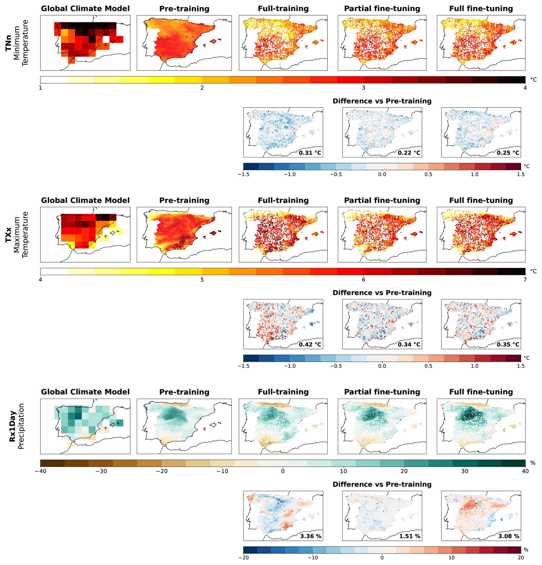
Figure 6 Climate change signals corresponding to the EC-Earth3-Veg model for the annual minimum of daily minimum temperatures (TNn), the annual maximum of daily maximum temperatures (TXx), and the annual maximum daily precipitation (RX1day). Each index is shown in a separate row, displaying the climate model's signal as well as the downscaled signals from the pre-trained model and the three different training regimes for the STATIONS-IBEB dataset (fully-training, partial fine-tuning and full fine-tuning), in columns. For each index, we also show the difference between the pre-trained model (over the grid points closest to the ROCIO-IBEB stations) and the three training regimes. For each of these differences, the spatial mean of the absolute differences is reported in the bottom-right corner.

To assess the variability of the resulting climate change projections, we train the DeepESD model ten times under each of the three different regimes, changing only the random initialization of the parameters. In the fully-trained model, all parameters are randomly reinitialized for each replica, whereas in the two fine-tuning regimes, only the parameters of the final dense layer are reinitialized. Figure 7 shows the standard deviation of the climate change signals for the TNn, TXx, and Rx1Day indices (rows) across model replicas for each training regime (columns). As expected, the fully-trained model exhibits the highest variability as no parameters are fixed, increasing the sources of variation across replicas. In contrast, although the fully fine-tuned model updates all parameters, it begins each training with the same initialized feature extractor, reducing variability across replicas. This effect is even more pronounced in the partially fine-tuned model, where the feature extractor is kept fixed and only the dense layer is trained. For temperature indices, both fine-tuning regimes show similar low variability. However, for precipitation, the fully fine-tuned model shows greater variability than the partially pre-trained one, particularly in southeastern Spain.

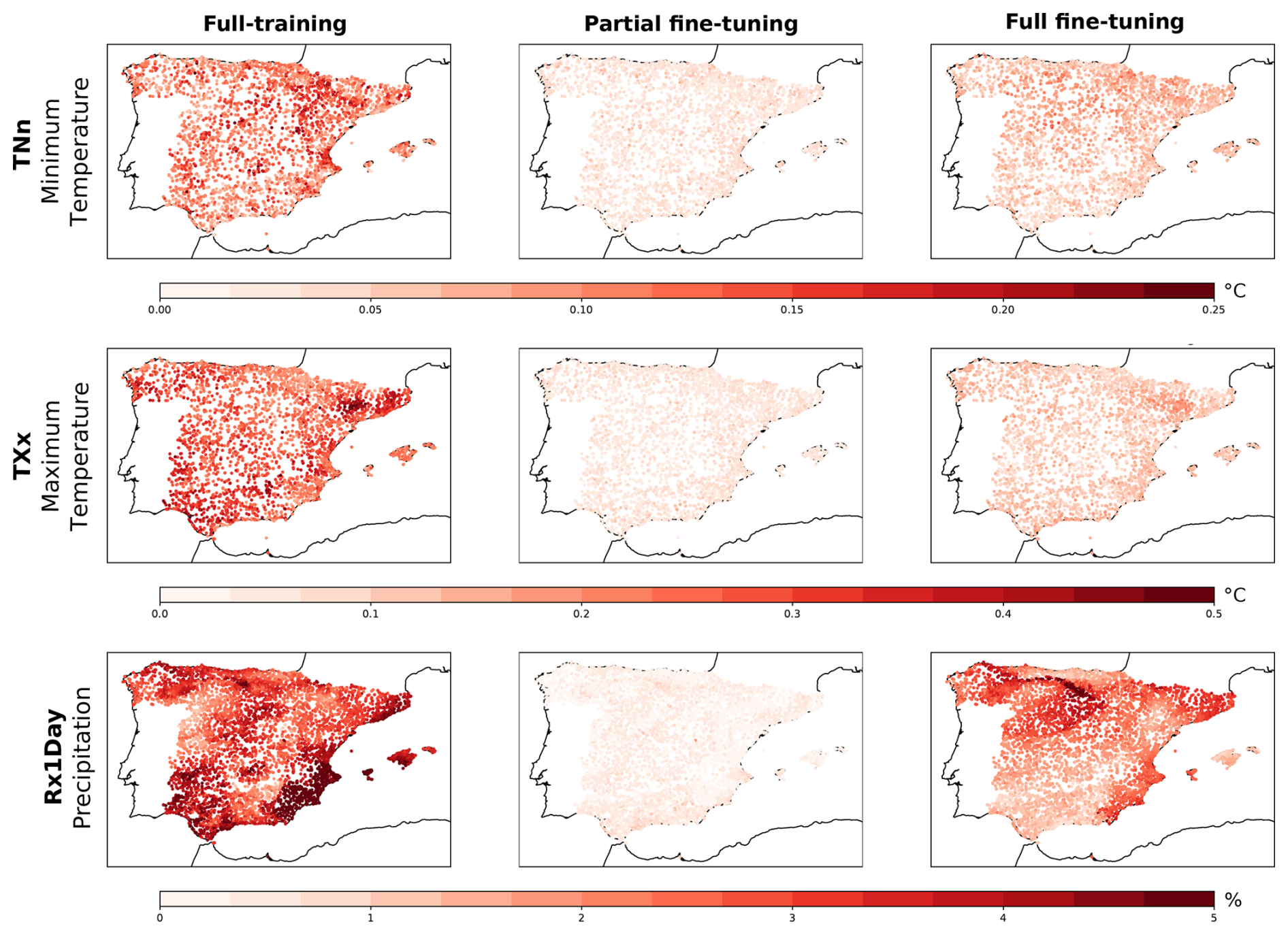
Figure 7 Standard deviation of the climate change signals for the TNn, TXx, and RX1Day indices (shown in rows), computed across ten training replicas under the fully-training, partial fine-tuning and full fine-tuning regimes on STATIONS-IBEB. The standard deviation for temperature signals is expressed in °C, while that for precipitation signals is given as a percentage.

4.4 Sensitivity to data record length

To evaluate whether the relationships learned by the pre-trained model are beneficial when data availability is limited, we train the aforementioned DL models on different versions of the STATIONS-IBEB dataset, each featuring a distinct proportion of missing data points. These versions are created by randomly removing observations across both space and time. During training, the DL models update their parameters only taking into account the non-missing data points of the predictand, which enables them to learn even when portions of the dataset are missing. Despite this partial data availability, the model retains the same architecture as the one trained without missing points, and thus can still generate predictions across the entire predictand domain.

In Fig. 8, we present the Root Mean Squared Error (RMSE) on the test set for the three downscaled variables under the different training regimes. Each regime is trained on versions of the STATIONS-IBEB dataset with varying percentages of artificially introduced missing values, shown on the x axis of each subplot. Note that the RMSE is computed on the test partition without missing data, enabling us to evaluate the model's ability to extrapolate to data points that were partially missing during training. Overall, the transferred relationships from the pre-trained model prove beneficial in low-data regimes, as evidenced by the improved performance of fine-tuned models compared to training from scratch. For both minimum and maximum temperatures, the fine-tuned regimes achieve lower RMSE values than the fully-trained regime, converging to the same value when the training is carried out on the STATIONS-IBEB dataset without missing data. The advantage of transferring pre-learned representations is especially pronounced under high missing-data regimes (e.g. 90 %), where these relationships aid in generalizing to unseen data points. For precipitation, a similar trend is observed between the fully-training and both fine-tuning regimes, however, the fully fine-tuned model performs worse than the others when more than 60 % of the training data is missing, though it still outperforms the fully-trained model beyond this threshold.

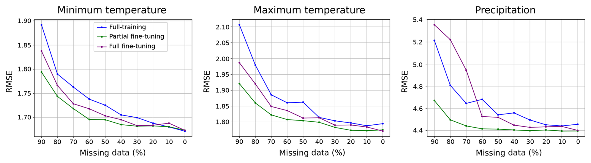
Figure 8 Root Mean Squared Error (RMSE) computed over the test set for three different training regimes (fully-training, partial fine-tuning and full fine-tuning), shown for the three downscaled variables (minimum temperature, maximum temperature and precipitation), in columns. Each model is trained on a different version of the STATIONS-IBEB dataset, varying in the proportion of artificially introduced missing data (indicated on the x axis of each subplot). Note that the RMSE shown here is computed using the STATIONS-IBEB test partition without missing data.

4.5 Application to a regional dataset

Finally, we extend the analysis of the proposed methodology to the STATIONS-CAT dataset. As discussed in Sect. 2.1.1, this dataset exemplifies a common use case motivating this approach: a regional, station-based observational dataset with limited temporal coverage. In contrast to STATIONS-IBEB, which is partially used to construct the ROCIO-IBEB gridded dataset, STATIONS-CAT comprises an independent set of stations over Catalonia and has no relation with ROCIO-IBEB. For STATIONS-CAT, data availability for all stations begins in 2009. Consequently, the fine-tuning regimes are trained using data from only the 2009–2019 period, while the test set covers 2019–2021. This experimental setup reflects one of the main challenges in regional statistical downscaling, namely the scarcity of long, homogeneous observational records. For the sake of clarity, the analysis in this section focuses on precipitation, which is generally considered the most challenging variable to downscale (Rampal et al., 2024; González-Abad, 2025a). The pre-trained model based on the ROCIO-IBEB dataset is the same as that used in the previous analysis with STATIONS-IBEB, and the training configurations for the full-training, partial fine-tuning and full fine-tuning regimes remain unchanged.

We begin by evaluating the performance of the different training regimes for the STATIONS-CAT dataset, focusing on extreme precipitation. Figure 9 shows the histogram of precipitation (with a logarithmically scaled y axis) computed over the test set across all STATIONS-CAT stations for the observations (STATIONS-CAT), the full-training, partial fine-tuning, and full fine-tuning models. For reference, we also include the histogram of the ROCIO-IBEB grid points and the pre-trained model output at the locations closest to the STATIONS-CAT stations. All models exhibit a comparable underestimation of the most extreme precipitation values, which is a well-known limitation of DL models trained with deterministic loss functions (González-Abad and Gutiérrez, 2025) and is not specific to any particular training regime. Importantly, the fine-tuned models do not show degraded performance relative to the fully-trained model, confirming that fine-tuning preserves station-scale predictive performance for extremes, consistent with the results observed for STATIONS-IBEB in Sect. 4.1.

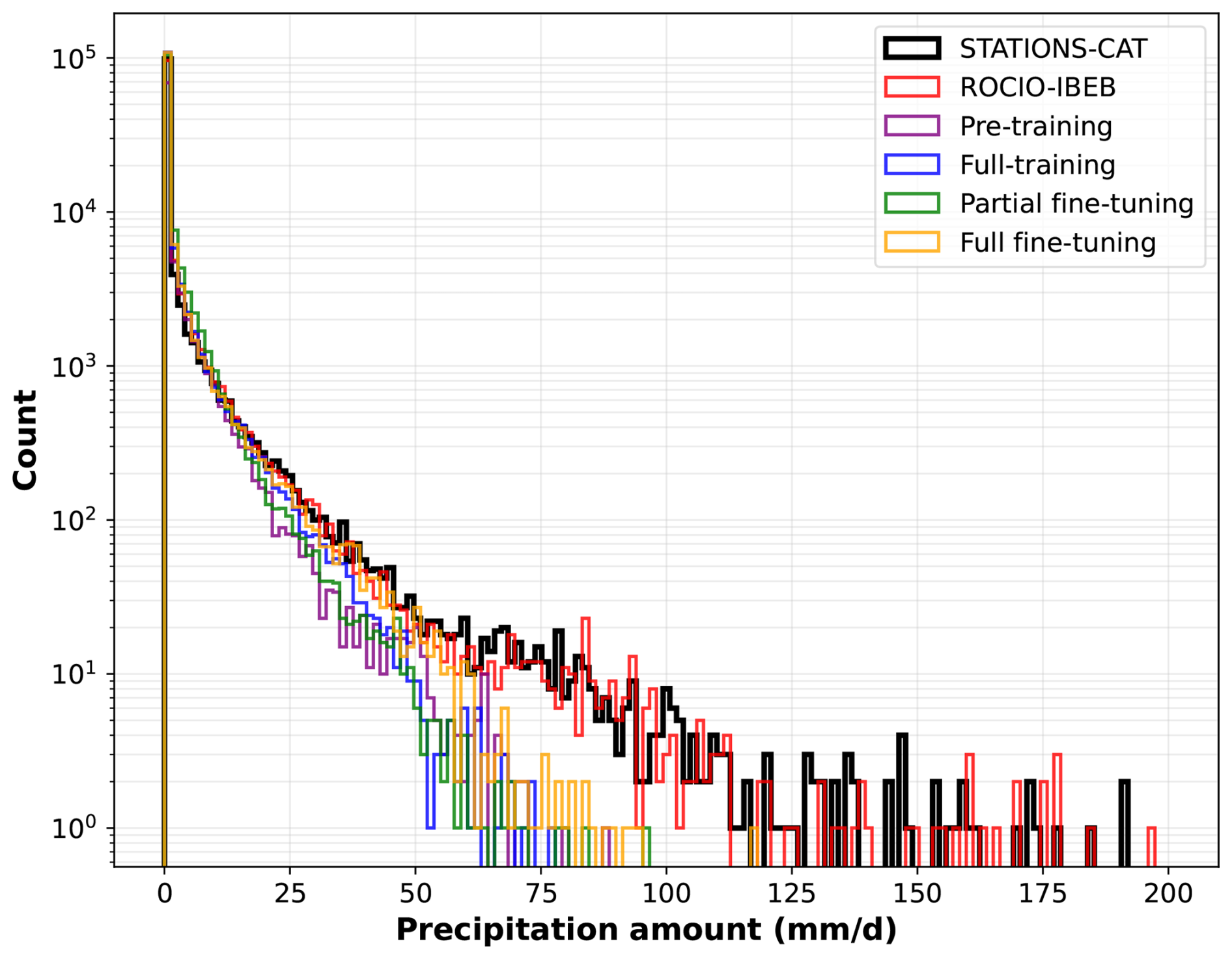
Figure 9 Histogram of precipitation over the test set (2019–2021) across all STATIONS-CAT stations for the observations (STATIONS-CAT) and the full-training, partial fine-tuning, and full fine-tuning models. The histogram for the ROCIO-IBEB grid points and the pre-trained model output at the locations closest to the STATIONS-CAT stations is also shown. Note that the y axis is logarithmically scaled to emphasize the tail of the distribution.

As in Sect. 4.2, Fig. 10 shows the ASM for the pre-training model (on ROCIO-IBEB) and the full-training, partial fine-tuning, and full fine-tuning regimes for STATIONS-CAT (for precipitation downscaling). In this case, the ASMs for both datasets are computed over the period corresponding to the STATIONS-CAT test set (2019–2021). It is important to note that, for the pre-training model on ROCIO-IBEB, the ASM is computed using the same number of grid points as there are stations in STATIONS-CAT, selecting the grid points closest to each corresponding station. This ensures a fair comparison between the relationships exposed by these techniques. The ASM for STATIONS-CAT exhibits a pattern similar to that observed for STATIONS-IBEB, with relevance highly distributed across the different predictor variables. It is also noticeable that, despite covering different regions, the distribution of relevance across variables for the pre-trained model is broadly consistent with that shown in Fig. 5. Focusing again in Fig. 10, the ASMs for the full-training and the partial and full fine-tuning regimes display large discrepancies, indicating that models trained exclusively on STATIONS-CAT tend to learn relationships that are less aligned with the physical patterns encoded in the reference pre-trained model on ROCIO-IBEB.

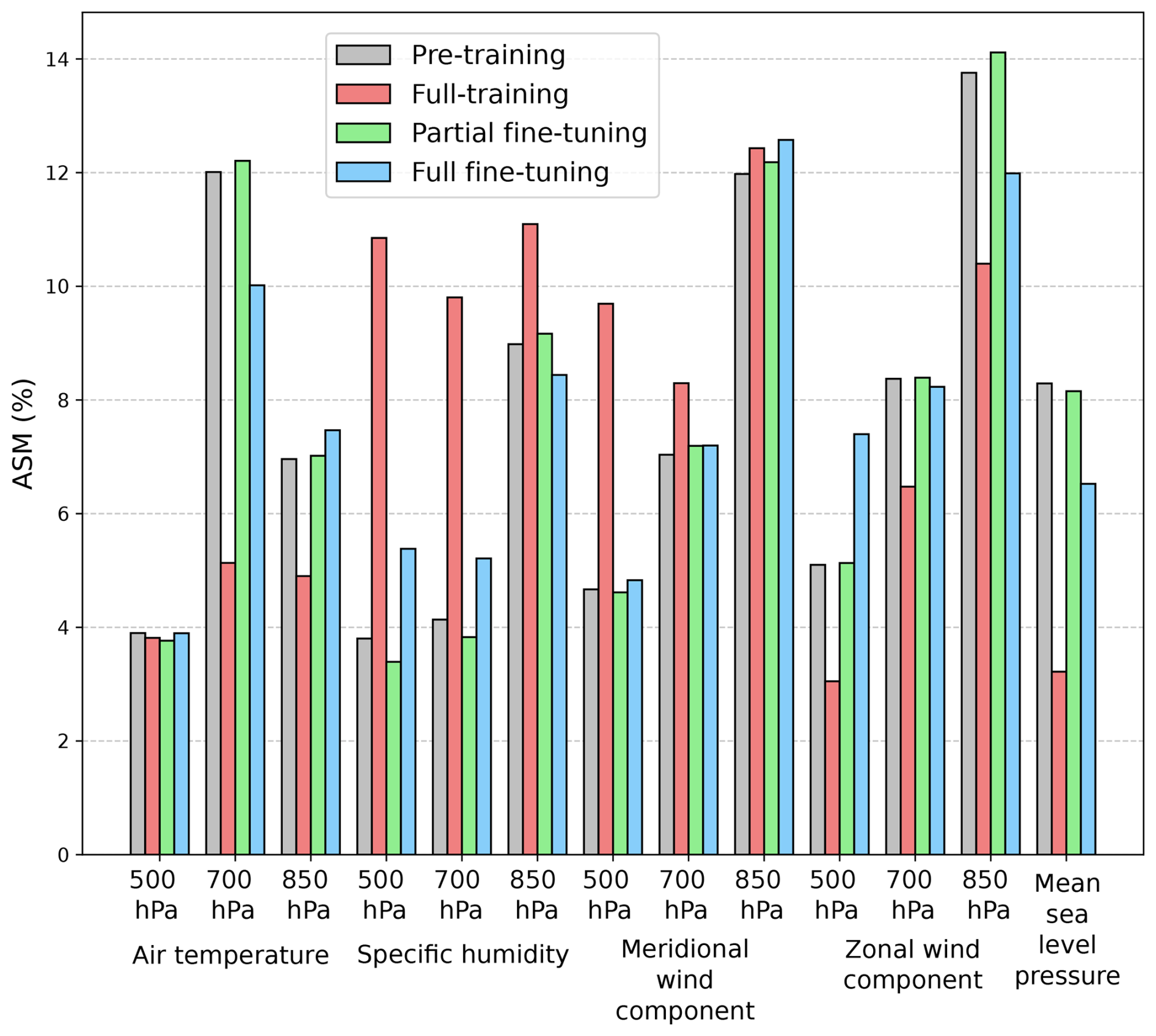
Figure 10 Same as Fig. 5, but for the full-training, partial fine-tuning, and full fine-tuning precipitation downscaling models applied to the STATIONS-CAT dataset over the test period 2019–2021. For the pre-trained model (on ROCIO-IBEB), the ASM is computed using the same number of grid points as there are stations in STATIONS-CAT, selecting the grid points closest to each corresponding station.

To illustrate the spatial distribution of relevance (i.e. the regions to which the model attends when making predictions for a specific station) we compute the saliency maps for the pre-training model (on ROCIO-IBEB) and the full-training, partial fine-tuning, and full fine-tuning models (on STATIONS-CAT) for a single station corresponding to Sabadell Airport. For the pre-training model, the saliency map is computed for the grid point closest to this station. Saliency maps are calculated for each day of the 2019–2021 period (the STATIONS-CAT test set), and then averaged to obtain the mean saliency for precipitation downscaling at this station. Figure 11 presents these average saliency maps for the four training regimes (shown in columns) and for four predictor variables (air temperature at 850 hPa, specific humidity at 700 hPa, meridional wind component at 850 hPa, and mean sea level pressure), shown in rows.

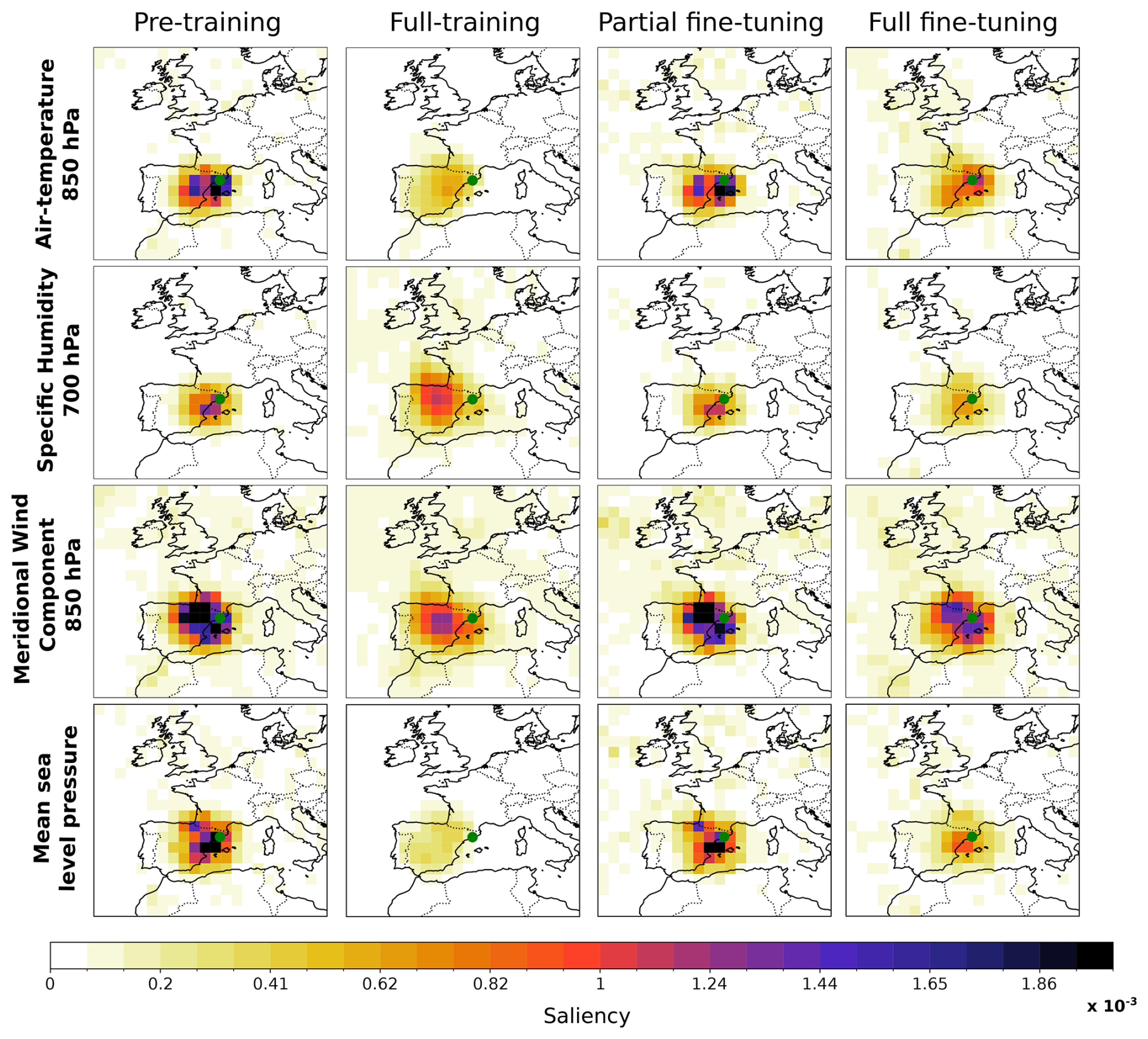
Figure 11 Saliency maps for the different training regimes: pre-training on ROCIO-IBEB, and full training, partial fine-tuning, and full fine-tuning on STATIONS-CAT (shown in columns), computed and aggregated over the STATIONS-CAT test period (2019–2021). Saliency maps are originally computed over all predictor variables but for clarity, we display only a subset of variables and a spatial domain centered on Catalonia. The variables shown (in columns) are air temperature at 850 hPa, specific humidity at 700 hPa, meridional wind component at 850 hPa, and mean sea level pressure. Saliency maps are computed with respect to the station indicated by the green point, corresponding to the Sabadell airport. For the pre-trained model the saliency maps are computed for the grid point closest to this station.

Overall, the saliency maps in Fig. 11 show that, for all models, the learned relationships are predominantly local, focused around the station being analyzed. This is expected for daily downscaling, as the physical processes governing local-scale precipitation dynamics generally occur within nearby regions. Comparing the spatial distribution of relevance across models reveals several interesting patterns. The saliency maps for the pre-training and partial fine-tuning models are highly similar, consistent with the discussion in Sect. 3: the important relationships are primarily learned by the feature extractor, while the final layer acts mainly as a linear calibrator. In contrast, the full fine-tuning model, in which the feature extractor weights are also updated starting from the pre-trained model, shows some changes in the spatial distribution of relevance. Nevertheless, the expected physical relationships are still captured, for example, the dependence of precipitation in Catalonia on conditions over the Mediterranean. By comparison, the full-training model, trained solely on STATIONS-CAT, exhibits a different spatial distribution of relevance. It places more attention on regions in the central Iberian Peninsula, as seen, for example, in the saliency maps of specific humidity at 700 hPa and meridional wind at 850 hPa. This suggests that the relationships learned by the full-training model may deviate from the expected physical dynamics governing precipitation in the region, highlighting the value of pre-training in constraining the model toward physically plausible relationships.

To further examine how these spatial saliency patterns vary across geographically distinct station subsets, we compute the same saliency maps as in Fig. 11 but aggregated separately for stations grouped by distance to the coast. Figure 12 shows the resulting maps for stations close to the coast (<20 km, top) and far from the coast (>150 km, bottom), focusing on the meridional and zonal wind components at 850 hPa and mean sea level pressure. For coastal stations, all models concentrate saliency over the coastal region, consistent with the dominant role of onshore moisture advection and Mediterranean wind flow in driving coastal precipitation. For inland stations, the pre-trained and fine-tuned models show a displacement of the meridional wind saliency beyond the station locations toward the Bay of Biscay, while the zonal wind and mean sea level pressure saliency shift only modestly, in proportion to the station displacement. This indicates that the model captures a physically relevant distinction: meridional flow channeled through the Bay of Biscay plays a specific role in inland precipitation that is less important for coastal stations. The full-training model does not exhibit this differentiated behavior, instead, its zonal wind saliency extends into western France and beyond, regions with no direct physical link to daily precipitation in Catalonia, further suggesting that training from scratch on limited data leads to less physically grounded spatial relationships.

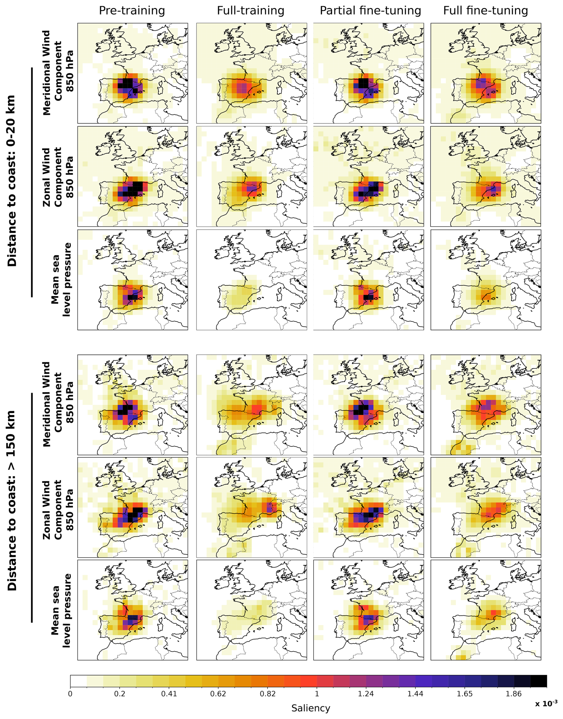
Figure 12 Same as Fig. 11 but computed separately for two groups of stations stratified by distance to the coast: coastal stations (<20, top) and inland stations (>150 km, bottom). For the sake of clarity, only the meridional and zonal wind components at 850 hPa and mean sea level pressure are shown. Saliency maps are aggregated over all stations within each group and over the STATIONS-CAT test period (2019–2021).

To complement the aggregated saliency analysis, we examine the saliency patterns for individual extreme precipitation events, comparing the full-training and full fine-tuning models. Figure 13 presents a case study for 21 January 2020 (within the test set), a day corresponding to a widespread extreme precipitation event (exceeding the 99th percentile at the analyzed station) affecting the broader Catalonia region. The first column shows the observed (ground-truth) and downscaled precipitation fields for both models. The remaining columns display, for each model, the wind vector fields (arrows) at 500, 700, and 850 hPa, with specific humidity shown in the background. The highlighted regions in the wind vector panels indicate the areas most influential for the model when downscaling precipitation at the target station (marked by a red box in the precipitation panels and a red triangle in the saliency panels), computed as the aggregated saliency from the wind components. Both models underestimate the observed extreme, but the full fine-tuning model shows a smaller underestimation. More importantly, the saliency patterns reveal a qualitative difference: the full-training model attributes relevance to a region where the wind field is not oriented toward the target station, indicating a spatial misalignment with the expected synoptic forcing. In contrast, the full fine-tuning model concentrates its saliency near the station, with wind vectors oriented toward it, consistent with moisture advection driving the precipitation event. We performed the same analysis for a localized extreme event (not shown) characteristic of convective precipitation. As expected, neither model captures this event, since isolated convective processes arise at scales finer than those resolved by the large-scale predictor fields. However, the full-training model exhibits highly dispersed saliency with no clear spatial structure, whereas the full fine-tuning model maintains a more concentrated pattern near the station, indicating that fine-tuning preserves physically plausible spatial relationships even when the prediction itself fails.

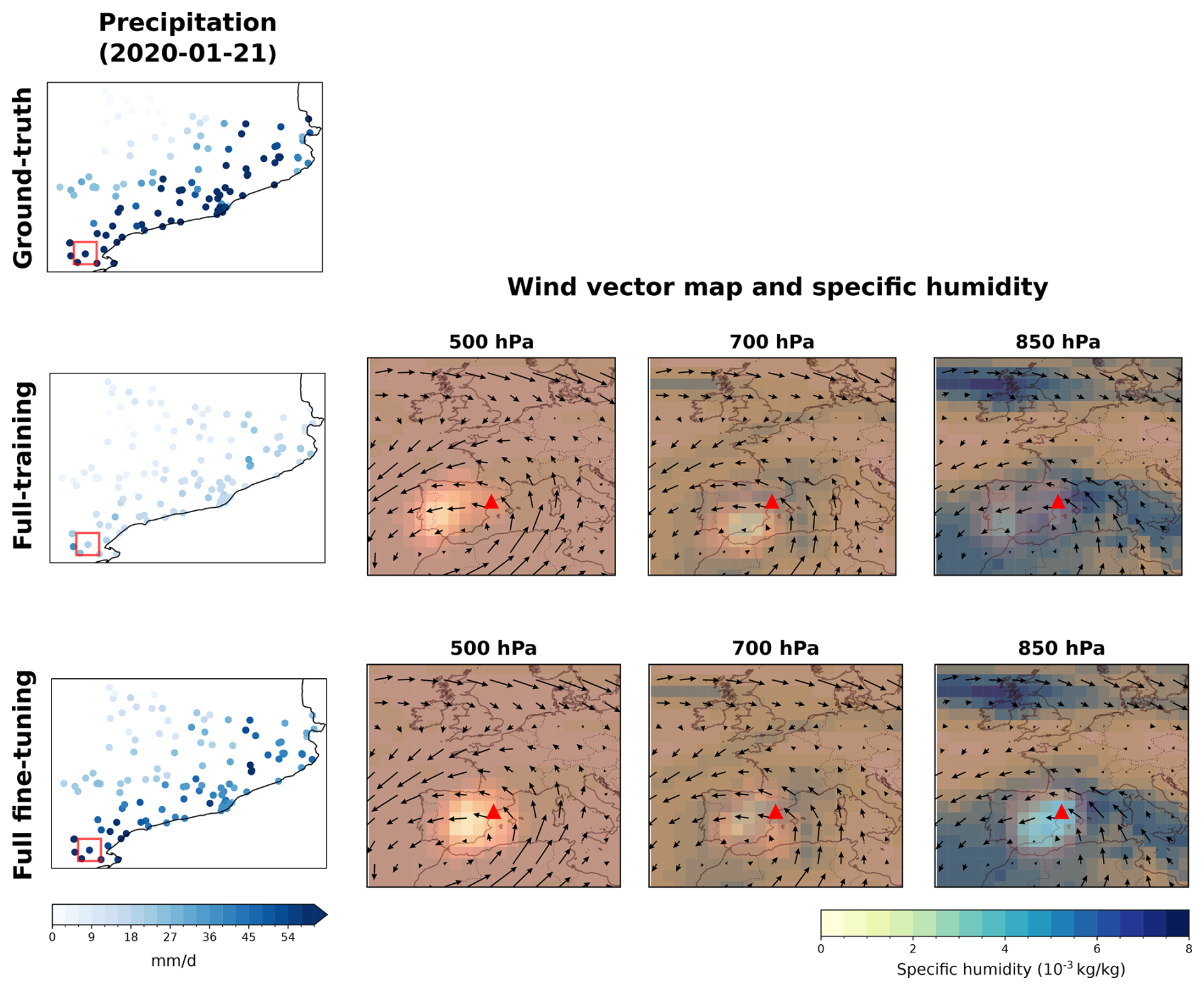
Figure 13 Case study for a widespread extreme precipitation event on 21 January 2020. The first column shows the observed (ground-truth) and downscaled precipitation fields for the full-training and full fine-tuning models on STATIONS-CAT. The remaining columns show, for each model, the wind vector fields (arrows) at 500, 700, and 850 hPa computed from the zonal and meridional wind components, with specific humidity displayed in the background. The highlighted (brighter) regions indicate the areas most influential for the model when downscaling precipitation at the target station, marked by a red box in the precipitation panels and a red triangle in the wind vector panels. This highlighted region corresponds to the aggregated saliency from the wind components used to compute the wind vectors.

Finally, in Fig. 14 we present the same analysis as in Fig. 7 (the standard deviation of the climate-change signal across training replicas) focusing specifically on the RX1Day index for precipitation. Similar to the results for STATIONS-IBEB, both fine-tuning regimes reduce the variability of the climate change signal across replicas, with partial fine-tuning achieving notably low variation. The full fine-tuning regime shows intermediate variability, higher than the partial fine-tuning but lower than full-training, with elevated variability particularly in the northwestern region corresponding to the Pyrenees Mountains.

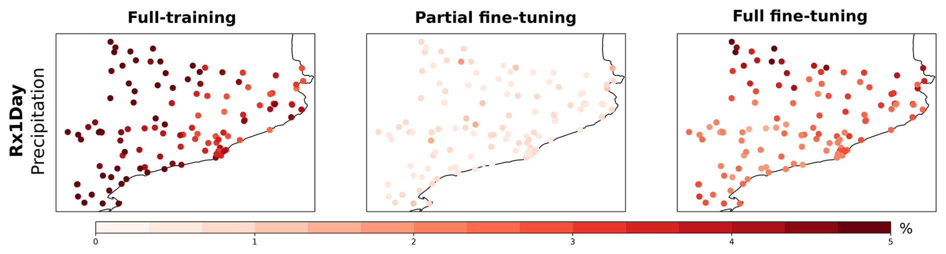
Figure 14 Same as Fig. 7 but for the fully-training, partial fine-tuning and full fine-tuning regimes on STATIONS-CAT dataset.

5 Discussion

The results presented in this work demonstrate the potential of pre-training for PP downscaling, particularly for developing a standard model in the region of Spain. As clarified in the introduction, the primary objective of this approach is not to maximize predictive skill on individual datasets, but rather to ensure consistency with a standard reference model while enhancing the robustness of climate projections across different regional datasets.

A key contribution of this work lies in demonstrating how fine-tuning facilitates the transfer of learned representations from the pre-trained model to models trained on regional datasets. As shown in Sect. 4.1, the performance metrics for STATIONS-IBEB across the three training regimes (full-training, partial fine-tuning, and full fine-tuning) are comparable. However, this similarity in skill masks a more fundamental difference: the fine-tuned models inherit the physical relationships encoded in the pre-trained model, whereas the fully-trained model learns its own set of relationships that may diverge from the established baseline. This inheritance of learned representations is particularly valuable when working with limited or regional datasets, where models trained from scratch are more susceptible to overfitting and learning spurious patterns.

The application to the STATIONS-CAT dataset provides evidence for the value of this approach in realistic operational scenarios. This regional dataset, covering only Catalonia with limited temporal coverage (2009–2021), exemplifies the typical challenges faced when developing regional climate projections: fewer stations and shorter time periods. Under these conditions, models trained exclusively on STATIONS-CAT show substantial deviations in their learned relationships, as evidenced by both the ASM diagnostics (Fig. 10) and the saliency maps (Figs. 11, 12 and 13). The ASM for the full-training regime exhibits large discrepancies compared to the pre-trained model, indicating that with limited data availability, models may fit noise and learn relationships that are less aligned with known dynamics. In contrast, both fine-tuning strategies successfully transfer the representations learned on ROCIO-IBEB, maintaining physical consistency even when adapted to this independent regional dataset. This is also reflected in standard metrics (not shown), such as those presented in Figs. 3 and 4, where fine-tuned models tend to achieve slightly lower errors and biases.

When analyzing the patterns learned by the various models using the ASM diagnostic, we find differences in the distribution of relevance across predictors for the three downscaled variables. Focusing on minimum temperature, all models exhibit their highest relevance in air temperature and specific humidity at 850 hPa (the lowest level) and mean sea level pressure, although the fully-trained model also shows a relatively high relevance for the zonal wind component at 850 hPa. This finding aligns with previous studies (Baño-Medina et al., 2023; González-Abad et al., 2023), which indicate that, for temperature, the most critical variables are air temperature and specific humidity at 1000 hPa, alongside geopotential height at 1000 hPa – closely related to mean sea-level pressure in our setup. The fully-trained and fully fine-tuned models show the greatest deviation from the expected relevance distribution, particularly in the increased ASM assigned to mean sea level pressure by the fully fine-tuned model. Nonetheless, the overall relevance patterns remain broadly similar. In contrast, the partial fine-tuned model exhibits relevance distributions more closely aligned with those of the pre-trained model, suggesting that, for this variable, fine-tuning the feature extractor may introduce a divergence from the relationships learned by the pre-trained model.

The ASM diagnostic indicates a stronger relationship between mean sea level pressure and maximum temperature than with minimum temperature. This is consistent with our understanding of temperature variability. Maximum temperature is largely controlled by atmospheric circulation patterns and adiabatic warming, both of which are effectively captured by this predictor. In contrast, minimum temperature typically requires a more complex set of predictors due to the influence of local surface conditions, moisture availability and radiative cooling processes. This distinction aligns with the fundamental meteorological principles governing daytime heating and nighttime cooling, as well as with previous studies (Favà et al., 2016, 2018; Merino et al., 2018; Pérez and García, 2023) that have demonstrated a robust relationship between pressure-related variables and temperature variability over the Iberian Peninsula. Interestingly, recent work (Cariou et al., 2025) has shown that DL models can effectively reproduce daily temperature variations over Europe using only mean sea level pressure as input, thereby underscoring the strong influence of atmospheric circulation. This aligns with our XAI-based findings, which highlight the particular relevance of mean sea level pressure, especially for maximum temperature.

In the case of precipitation, relevance is distributed across the full set of predictor variables, which aligns with the fact that precipitation dynamics encompass a broader range of phenomena. As shown in Figs. 5 and 10, wind components play a significant role, particularly in northwestern regions, where westerly winds transport moisture from the Atlantic Ocean. The influence of both temperature and humidity also makes sense in this context; for example, higher temperatures require greater amounts of humidity to reach saturation, a key factor in precipitation events. Additionally, mean sea-level pressure is relevant because pressure differentials can trigger the lifting of moist air. Overall, while all training regimes agree on the distribution of relevance for STATIONS-IBEB, the partially fine-tuned model produces values that more closely align with those of the pre-trained model. For STATIONS-CAT, this alignment becomes even more critical, as the full-training model shows substantial deviations that suggest the learning of spurious relationships.

The spatial saliency maps presented in Fig. 11 provide further insight into the nature of these learned relationships. Overall, these maps show that for all models, the learned relationships are predominantly local, focused around the station being analyzed. This is expected for daily downscaling, as the physical processes governing local-scale precipitation dynamics generally occur within nearby regions, consistent with findings in previous work (González-Abad et al., 2023). The spatial saliency maps reveal that while both fine-tuning strategies maintain similarity to the pre-trained model's patterns, the full-training model exhibits notably different spatial distributions of relevance, placing more attention to the central Iberian Peninsula rather than the Mediterranean region expected for precipitation in Catalonia. This deviation highlights how training exclusively on limited regional data can lead to relationships that diverge from established dynamics, underscoring the value of pre-training in constraining models toward physically plausible patterns. When stratifying STATIONS-CAT by distance to the coast, the pre-trained and fine-tuned models show, unlike the full-training model, physically coherent shifts in their saliency patterns, concentrating near the Mediterranean for coastal stations and extending toward the Bay of Biscay for inland stations, consistent with distinct regional moisture pathways. This physical coherence is further confirmed by the case-wise analysis of an individual extreme precipitation event (Fig. 13). For a widespread extreme event, the full fine-tuning model concentrates saliency near the target station with wind vectors oriented toward it, consistent with the expected synoptic forcing, whereas the full-training model attributes relevance to spatially misaligned regions.

Regarding the climate change signals, the results for minimum and maximum temperature closely align with those reported in González-Abad and Gutiérrez (2025), indicating plausible projections. The lack of relevant differences among the signals from the different training regimes for STATIONS-IBEB may originate from the use of 30-year climatologies, suggesting that the choice between datasets does not fundamentally impact statistical trends at these temporal scales when sufficient data is available. However, the enhanced robustness provided by fine-tuning becomes evident when examining variability across training replicas. As expected, the partially fine-tuned model exhibits lower variability than the fully fine-tuned model, since fixing the feature extractor constrains the optimization process to a smaller region of the parameter space (Erhan et al., 2010). This is evident in Figs. 7 and 14, where the spread across replicas becomes nearly zero when the feature extractor is frozen. For STATIONS-CAT, this reduction in variability takes on particular significance: both fine-tuning regimes substantially reduce the variability of the climate change signal compared to full-training, with partial fine-tuning achieving notably low variation. This enhanced robustness can be attributed to the transfer of meaningful physical relationships from the pre-trained model, making fine-tuned models less susceptible to the spurious patterns that emerge when training exclusively on limited regional data, a reduction in epistemic uncertainty particularly valuable for developing reliable regional climate projections that maintain consistency with national-scale assessments.

As shown in Sect. 4.4, the benefits of transferring pre-learned representations are also evident in low-data regimes, where portions of the observational record are missing. The transferred relationships from the pre-trained model prove beneficial when data availability is limited, as evidenced by the improved performance of fine-tuned models compared to training from scratch. This advantage has been previously observed in the super-resolution field (Zhu and Zhou, 2024), where pre-trained models have successfully transferred relationships across different regions. However, in super-resolution, regional transferability is more straightforward since the model learns an interpolation function by relying on a coarser version of the predictand. In contrast, in the PP approach, the empirical relationships being learned may depend on dynamic regional phenomena, making the successful transfer demonstrated here particularly noteworthy.

6 Conclusions

Current statistical downscaling methodologies often involve different research groups employing various schemes and drawing on datasets of varying spatial resolution and temporal coverage; this can lead to inconsistencies in the resulting downscaled projections. Such discrepancies pose challenges when nationwide products exist – for example, Escenarios-PNACC 2024 in Spain. To address this issue, we introduce pre-training as a strategy to develop a standard DL model for PP downscaling in Spain, with the explicit goal of ensuring consistency and enhancing robustness when adapting to different regional datasets. Specifically, we propose a standard model using the DeepESD architecture trained on the ROCIO-IBEB gridded dataset as the foundation. We then demonstrate how this model can serve as a basis for training on point-based datasets through two fine-tuning approaches: partial (freezing the feature extractor) and full (allowing the feature extractor to adapt).

As demonstrated by our XAI-based analysis, the pre-training paradigm enables fine-tuned models to inherit the physical relationships learned by the pre-trained model, grounding their climate projections in a consistent physical basis. In the case of Spain, these inherited relationships align with previous findings in the literature (Baño-Medina et al., 2021; González-Abad et al., 2023), and the fine-tuned versions successfully preserve them even when adapted to independent regional datasets. This inheritance is particularly valuable when working with small regional datasets, where DL models trained from scratch are prone to overfitting and learning spurious patterns, as evidenced by our results with STATIONS-CAT. The application to this regional Catalonian dataset exemplifies the typical operational scenario motivating this work: developing regional climate projections that maintain coherence with established national products while accommodating local observational data constraints.

Beyond ensuring consistency, leveraging an established downscaling model through fine-tuning reduces the epistemic uncertainty in climate projections. By constraining the parameter search space and transferring meaningful representations, fine-tuning strategies lead to more robust projections with reduced variability across model initializations. This is particularly evident in the climate change signals for both STATIONS-IBEB and STATIONS-CAT, where fine-tuning substantially decreases the spread across training replicas compared to training from scratch. When the pre-trained model is proven reliable, this reduction in uncertainty further enhances trust in regional projections and ensures their alignment with national assessments. Importantly, the XAI-based analysis also demonstrates that the pre-trained relationships remain physically interpretable across different geographically station subsets, with fine-tuned models exhibiting spatially coherent saliency patterns more consistent with known regional dynamics whereas models trained from scratch on limited data show less physically grounded spatial saliency.

Our work also reveals additional benefits of pre-training in the context of PP downscaling. In low-data regimes – where datasets often have missing observations due to station errors or limited temporal coverage – fine-tuning allows DL models to rely on pre-learned representations rather than attempting to extract all relationships from sparse local data. This is especially valuable in regional contexts, where incomplete or inconsistent datasets are common. Furthermore, fine-tuning does not degrade station-scale predictive performance relative to full training, including for extreme precipitation, ensuring that the benefits of representational consistency come without sacrificing performance.

The promising results of pre-training in the context of PP downscaling open several avenues for future research. In the case of Spain, one potential approach to creating a more representative basis model is to leverage the range of available observational datasets (Peral García et al., 2017; Herrera et al., 2019), which are generated using various methods (e.g. different interpolation techniques). Integrating multiple datasets could help reduce observational uncertainty tied to dataset selection. Another promising direction is to extend this approach to larger regions, such as Europe, where multiple observational datasets are also available. In such continental regions, downscaling models are typically trained on continental or global observational datasets that may not reflect the specific properties of individual regions. In this case, a standard model could be trained on broader datasets and then fine-tuned with regional datasets at higher resolutions, further enhancing its accuracy and applicability in generating nationwide products while maintaining consistency across scales. Lastly, following efforts both within Lessig et al. (2023); Nguyen et al. (2023); Bodnar et al. (2025) and beyond Bommasani et al. (2021) the climate and weather domains, a self-supervised learning strategy could be employed to train a foundational model by drawing on data from GCMs and Regional Climate Models (RCMs) (Rampal et al., 2024). Such a foundational model could then serve as a basis for numerous regions, variables, and even different downscaling tasks (e.g. PP downscaling or RCM emulation).

Overall, pre-training emerges as a valuable strategy for developing consistent and robust regional climate projections. By fine-tuning a reliable pre-trained model, we can ensure that regional projections inherit established physical relationships, maintain coherence with national-scale assessments, and exhibit reduced epistemic uncertainty in critical extrapolation scenarios, such as downscaling GCMs under future climate conditions. The successful application to STATIONS-CAT demonstrates that this approach is particularly beneficial for the typical operational scenario: adapting a standard national model to limited regional datasets while preserving physically meaningful relationships and enhancing projection robustness. These advantages position pre-training as a valuable avenue for future research, potentially enabling robust standard models that a wider community of users and researchers can readily adopt for developing consistent multi-scale climate projections.