Surface horizontal kinetic energy sensitivity to numerical parameters in tidal-resolving North and Equatorial Atlantic simulations

Surface horizontal kinetic energy (SHKE) reflects the distribution of ocean circulation across temporal and spatial scales, shaping energy transfer and mixing in the upper ocean. Quantifying both total SHKE and its frequency content helps characterize processes from low-frequency motions to tides and near-inertial waves, but SHKE variability is difficult to quantify with observations alone. High-resolution tidal-resolving ocean models can bridge gaps in our understanding, yet the modeling results depend on the realism of the configuration choices. In this study, we isolate the role of individual model parameters by comparing seven tidal-resolving HYbrid Coordinate Ocean Model (HYCOM) simulations of the North and Equatorial Atlantic, in which only one parameter is varied at a time. Surface drifters serve as the observational reference and numerical drifters are seeded in the reference experiment to quantify the distortion of the low frequency and tidal variance introduced by the Lagrangian sampling. This framework allows a controlled sensitivity analysis of the SHKE distribution across four frequency bands, separately for deep ocean and continental shelf waters. The experiments show that, within the range of configuration changes explored, horizontal resolution is the dominant control of offshore total SHKE whereas vertical refinement has a smaller impact offshore and a slightly stronger one on the shelf. Hourly wind forcing strongly amplifies the diurnal and near-inertial variability, finer bathymetry enhances the offshore semidiurnal energy, and internal wave drag controls the tidal-band energy equatorward of their critical latitudes while leaving the low-frequency motions nearly unchanged. Increasing the number of tidal-constituent from one (M₂) to eight of the largest constituents sharply increases the diurnal SHKE and allows us to disentangle the tidal from the non-tidal fraction of the diurnal cycle. Taken together, these experiments show that the shelf and offshore subdomains respond differently to each parameter and that each frequency band is sensitive to a different set of parameters. These results quantify how the configuration choices shape the modeled total SHKE and its spectral distribution, and offer guidance for setting up high-resolution tide-resolving model experiments.

1 Introduction

Advances in observations and remote sensing have dramatically improved the characterization of ocean velocity fields. For example, geostrophic velocities derived from altimetry provide a global perspective on the geostrophic component of the surface kinetic energy, and have yielded important insights into large-scale to mesoscale motions and their variability (Le Traon, 2013; Abdalla et al., 2021). However, despite recent advances such as the Surface Water and Ocean Topography (SWOT) mission (Morrow et al., 2019; Fu et al., 2024; Archer et al., 2025; Villas Bôas et al., 2025), the spatial and temporal resolution of altimetry remains insufficient to fully resolve smaller oceanographic features and higher frequency motions (< 100 km, < days). Observations of velocities from ADCPs and drifters can capture higher-frequency motions (∼ hourly), but these observations are typically limited in duration and geographically sparse.

The advancement of computational capacity has allowed large-scale high-resolution numerical models to include submesoscale motions (Chassignet and Xu, 2017; Ajayi et al., 2020, 2021; Chassignet et al., 2023) and tides (Arbic et al., 2012, 2018; Buijsman et al., 2020; Arbic, 2022; Xu et al., 2022). Numerical models therefore provide a complementary tool to study processes at high temporal and spatial resolution. These models are particularly relevant for the study of high-frequency motions such as internal tides, near-inertial waves, and motions spanning quasi-inertial to low-frequency motions. However, numerical models are, by construction, truncated representations of the ocean, and the modeled circulation is strongly dependent on parameter choices, such as mixing parameterizations and/or horizontal and vertical resolution (e.g., Chassignet and Xu, 2017; Buijsman et al., 2020; Chassignet et al., 2023; Xu et al., 2023; Hiron et al., 2025; Buijsman et al., 2025).

Spectral decomposition of surface currents provides a powerful framework to separate and analyze the distribution of surface horizontal kinetic energy (SHKE) across physically meaningful frequency bands. This approach enables the investigation of key interactions (e.g., wave–current coupling, nonlinear wave–wave transfers), the pathways of energy across scales, and even the tuning of model parameters. Elipot and Lumpkin (2008) and Elipot et al. (2016) first applied rotary spectra to drifter observations, decomposing SHKE into anticyclonic and cyclonic components that could be mapped into distinct reservoirs of variability to quantify the near surface variability on global scales. Extending this method to model–observation comparisons, Yu et al. (2019) compared a global MIT General Circulation Model (MITgcm) simulation (LLC4320) to surface drifters in waters deeper than 500 m and demonstrated that surface drifters are an efficient database for assessment of the surface circulation predicted by a tide- and eddy-resolving global ocean model. Indeed, they found similar qualitative patterns in SHKE in both the model and observations, with a dominance of low frequencies and well-defined tidal and near-inertial peaks. Quantitative differences, however, emerged, such as energy deficit (e.g., at low latitudes, and at the near-inertial frequency) or excess (e.g., at the semidiurnal frequency) in the model relative to the observations. Subsequently, Arbic et al. (2022) compared the near-surface SHKE of another high-resolution global simulation performed with the Hybrid Coordinate Ocean Model (HYCOM) to that of the MITgcm LLC4320 and the drifters' SHKE. The analysis focused on the vertical structure of the near-surface current by comparing results at the surface with those at 15 m depth. They found significant differences between surface and 15 m velocities in all frequency bands, except the semidiurnal band. The same energy deficit as in Yu et al. (2019) remained present in the models near the equator when compared to observations, but the lack of energy at the near-inertial frequency was less pronounced in HYCOM than in the MITgcm. In addition, the HYCOM semidiurnal SHKE was found to be closer to estimates derived from surface drifter observations than the MITgcm semidiurnal SHKE. Although both Yu et al. (2019) and Arbic et al. (2022) put forward several explanations for the differences between the modeled SHKE and the SHKE derived from surface drifter data, they acknowledged the inherent difficulty of comparing fields derived from Eulerian (models) and Lagrangian (observations) velocities. Arbic et al. (2022) also pointed out several limitations in their ocean model comparison, i.e., different forcing and numerical parameters (e.g., vertical grid resolution, frequency of atmospheric wind forcing, presence or absence of wave drag), outputs from different years, and systematic model errors (e.g., issues with the tidal forcing in the MITgcm LLC4320 simulation). These limitations illustrate the difficulty of disentangling the respective roles of individual parameters when simulations differ simultaneously in multiple aspects, leaving open the question of which choices most strongly shape the modeled SHKE.

In addition to parameter-related uncertainties, there is the distortion in SHKE that arises when estimating the low frequency and tidal variance from drifters (Zhang et al., 2024; Caspar-Cohen et al., 2025). Zhang et al. (2024) systematically compared Eulerian and Lagrangian estimates of SHKE by seeding a large ensemble of numerical drifters into the global MITgcm LLC4320 using the v2.0 Parcels Python package (Lange and Van Sebille, 2017; Delandmeter and Van Sebille, 2019) and showed that Lagrangian velocity spectra are generally smoother and tend to underestimate SHKE at low-frequency and in tidal bands, particularly in regions with strong low-frequency SHKE. Caspar-Cohen et al. (2025) systematically compared the Lagrangian and Eulerian frequency distributions in LLC4320 and confirmed the findings of Yu et al. (2019) and Arbic et al. (2022), i.e., that the semidiurnal energy in MITgcm LLC4320 is, on average, about twice the observed values and that HYCOM shows relatively minimal bias overall, though regional variations are apparent.

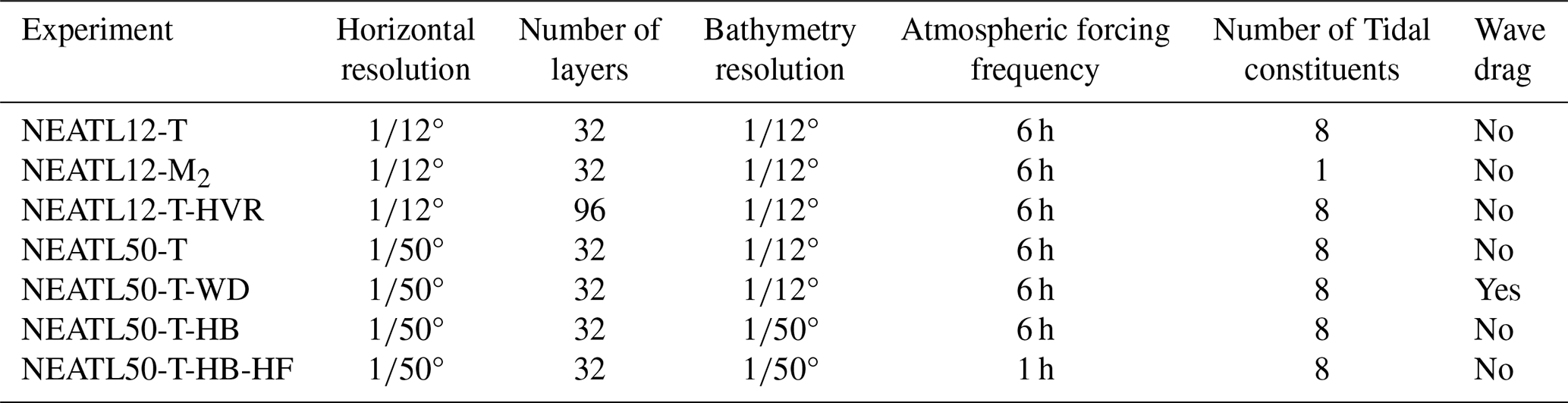
In summary, the above studies highlight two main sources of ambiguity in their model–observation comparisons of SHKE: the simultaneous variation of multiple parameters between simulations, which prevents a clean attribution of SHKE differences to any specific choice, and the distortion introduced by Lagrangian sampling, which complicates the direct use of drifter observations as a reference. In this paper, we remove these ambiguities by (a) analyzing a series of experiments in which only a single parameter is varied at a time and (b) using numerical drifters to evaluate the level of agreement between the model and the observations and to quantify the bias arising from Lagrangian sampling. The central objective of the paper is to isolate and quantify the impact of the choices in numerical and forcing parameters on the modeled SHKE. This is achieved by relying on a suite of tidal-resolving HYCOM simulations of the North and Equatorial Atlantic (Table 1) that allows us to directly attribute SHKE differences to (a) grid resolution (horizontal and vertical), (b) bathymetry resolution, (c) forcing (wind frequency and tidal content), and (d) wave drag. This framework also enables us to extend the analysis from offshore/deep ocean waters (deeper than 500 m), covered by previous drifter-based comparisons, to inshore/continental shelf waters (shallower than 500 m), where the high-frequency SHKE is of particular importance, a region that surface drifter-based comparisons could not cover due to the lower density of observations. The Lagrangian comparison enables us to link the Eulerian-based sensitivity results directly to observations, without conflating genuine model biases with Lagrangian-Eulerian sampling differences.

The article is organized as follows: Sect. 2 describes the seven HYCOM simulations, the implementation of the numerical drifters, and the surface drifter database used in the comparison. It also introduces the method used to calculate the rotary spectra. In Sect. 3, the domain-averaged SHKEs from all Eulerian and Lagrangian datasets are compared within a common framework, providing a global view of the datasets and identification of the spectral features they share. This section serves as the baseline for the comparisons performed in the following sections. In Sect. 4, the Lagrangian spectral estimates from the numerical drifter experiment are compared to the drifter observations and to the Eulerian model outputs. This section provides the link between the surface drifter observations and the Eulerian experiments analyzed in the following section. Section 5 systematically quantifies the impacts of the configuration and parameter choices listed above on the SHKE using the Eulerian frequency rotary spectra, with separate analyses conducted for deep ocean and continental shelf waters. The final section synthesizes the results by discussing the parameters that most strongly affect the SHKE distribution in each frequency band and by addressing which one could be adjusted to reduce the model-drifter gap.

2 Data and methods

This section describes the datasets and methods used throughout this study. All analyses are conducted within the North and Equatorial Atlantic (NEATL) domain, which extends from 28° S to 80° N (Fig. 1a). The domain is divided into two subdomains: offshore/deep ocean waters and inshore/continental shelf waters, defined as 1°×1° cells whose median depth, estimated from the ETOPO1 database (Amante and Eakins, 2009), exceeds or is shallower than 500 m respectively. These two subdomains represent approximately 77 % and 23 % of the total NEATL domain area, respectively.

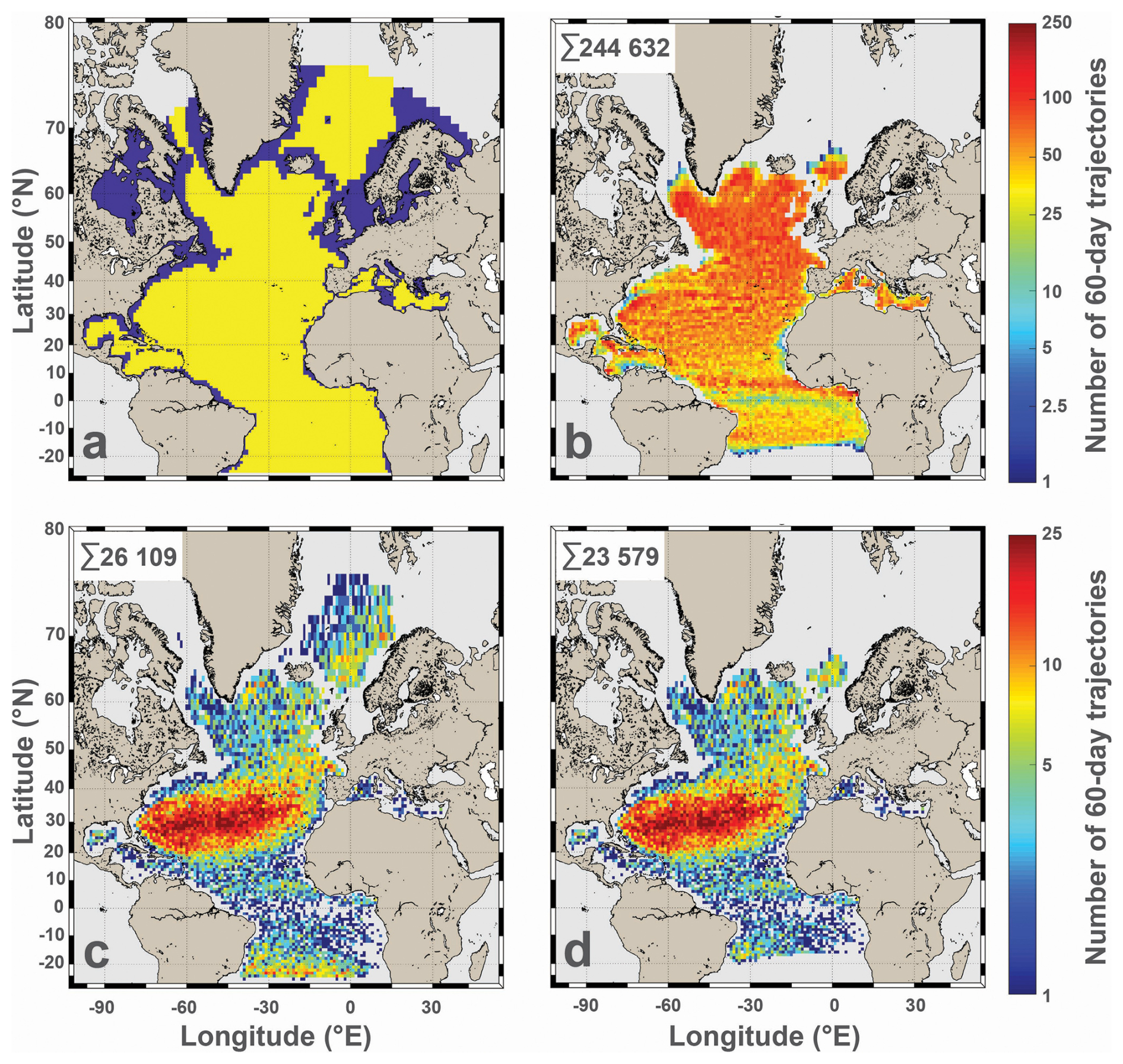
Figure 1 (a) HYCOM NEATL domain in 1°×1° bins of yellow (blue) regions indicating offshore (inshore) regions in waters deeper (shallower) than 500 m. (b–d) Number of 60 d trajectory segments per 1°×1°  offshore bin for (b) the full OceanParcels experiment (OP Seed 1/2°), (c) the undrogued surface drifter observations, and (d) the subsampled OceanParcels experiment (OP Seed Drifters), constructed to reproduce the spatial sampling of the observed undrogued drifters. The total number of segments is indicated in the upper-left corner of panels (b) to (d).

2.1 Ocean Surface Drifters

We use version 2.01 of the hourly data set from the Global Drifter Program (Elipot et al., 2016, 2022) which includes 15 m-drogued and undrogued drifters. It is important to note that the positioning system used to track the drifters (Argos or GPS) can have an impact on the power spectral density of velocity. Yu et al. (2019) showed that the noise in the Argos positioning system adds high-frequency energy when compared to surface buoys equipped with GPS. In the NEATL domain (Fig. 1a), the database of undrogued (drogued) drifters, which was downloaded on 30 April 2025, can be divided into 27 134 (25 956) continuous 60 d segments, each associated with its mean position over the segment duration. Among these, 11 591 (14 933) are from GPS-tracked drifters. Of the segments of both Argos and GPS-tracked undrogued (drogued) drifters, 26 109 (23 704), corresponding to 96 % (91 %) of the total, are located in offshore waters, reflecting the sparse coverage of surface drifters in coastal regions. Because SHKE is defined at the ocean surface, we focus on undrogued drifters in the following analyses, as they more accurately sample surface velocities (Niiler and Paduan, 1995; Lumpkin and Pazos, 2007). Undrogued drifters are known to carry a larger wind-slip error than drogued ones, reaching $\mathrm{8.6}\times {\mathrm{10}}^{-\mathrm{2}}$ m s⁻¹ per 10 m s⁻¹ wind speed compared to $\mathrm{0.7}\times {\mathrm{10}}^{-\mathrm{2}}$ m s⁻¹ downwind per 10 m s⁻¹ wind speed for drogued drifters (Niiler and Paduan, 1995), but this slip has not yet been comprehensively disentangled from genuine oceanic surface variability across frequencies (see Arbic et al., 2022, for a discussion of the limitations of using undrogued versus drogued drifters for model comparison). The number of undrogued drifter segments per 1°×1° cell in the offshore domain is shown in Fig. 1c. The spatial distributions of the other drifter datasets (drogued and undrogued, GPS-tracked and all) are provided in Fig S1 in the Supplement.

2.2 HYbrid Coordinate Ocean Model (HYCOM) simulations

The NEATL HYCOM experiments, covering the Atlantic from 28° S to 80° N (Fig. 1a), are part of a suite of eddying and submesoscale-enabled numerical simulations performed with HYCOM v2.3.01 (Bleck, 2002; Chassignet et al., 2003, 2009). These simulations (Chassignet and Xu, 2017; Xu et al., 2022; Chassignet et al., 2023; Xu et al., 2023) were performed to study and quantify the impact of horizontal and vertical resolution on the large-scale circulation and water mass transformations in the Atlantic. In this paper, we analyze three $\mathrm{1}/\mathrm{12}$° horizontal grid-spacing configurations (9 km at the equator, 6 km in the Gulf Stream region) and four $\mathrm{1}/\mathrm{50}$° horizontal grid-spacing configurations (2.25 km at the equator, 1.5 km in the Gulf Stream region). Three of these configurations have been used previously in Xu et al. (2022), while four simulations (NEATL12-T, NEATL12-M₂, NEATL12-T-HVR, and NEATL50-T-WD) are analyzed for the first time. The simulations are integrated for 18 months with tidal forcing of the eight largest tidal constituents (K₁, O₁, P₁, Q₁, M₂, S₂, N₂, and K₂) after spin-up as described in Xu et al. (2022). The last 12 months outputs are used in the analysis.

These simulations are listed in Table 1, but are described in more details in the following:

• NEATL12-T is the tidal $\mathrm{1}/\mathrm{12}$° reference simulation with 6-hourly atmospheric forcing and 8 tidal constituents.

• NEATL12-M₂ is a twin experiment of NEATL12-T, but with only the semidiurnal tidal constituent (M₂, 1.932 cycles per day (cpd)).

• NEATL12-T-HVR is a twin experiment of NEATL12-T, but with 96 vertical coordinates instead of 32.

• NEATL50-T is a twin experiment of NEATL12-T, but with a $\mathrm{1}/\mathrm{50}$° horizontal grid-spacing and a coarse bathymetry linearly interpolated from the $\mathrm{1}/\mathrm{12}$° grid-spacing topography of the NEATL12-T (Chassignet and Xu, 2017; Xu et al., 2022; Chassignet et al., 2023). NEATL12-T's bathymetry is based on the 2' Naval Research Laboratory digital bathymetry database, which combines the global topography based on satellite altimetry of Smith and Sandwell (1997) with several high-resolution regional databases.

• NEATL50-T-WD is a twin experiment of NEATL50-T. However, instead of having no wave drag as in NEATL50-T, a Jayne and St. Laurent (2001) internal wave drag with a multiplicative factor of 0.25 is applied to the bottom of the water column (we refer to Buijsman et al. (2015, 2020) for a discussion of this parameter).

• NEATL50-T-HB is a twin experiment of NEATL50-T, but with a $\mathrm{1}/\mathrm{50}$° bathymetry that is derived from the 2019 version of the 15 arcsec General Bathymetric Chart of the Ocean data set (GEBCO Bathymetric Compilation Group 2019, 2019) as in Chassignet et al. (2023).

• NEATL50-T-HB-HF is a twin experiment of NEATL50-T-HB, but with higher-frequency, hourly wind stress variability from the National Centers for Environmental Prediction Climate Forecast System Reanalysis (Saha et al., 2010) instead of the 6-hourly wind forcing used in previous experiments.

In the vertical dimension, the above simulations contain 32 or 96 hybrid layers with density referenced to 2000 m (σ₂) (see Chassignet and Xu, 2017 and Xu et al., 2023 for details). The vertical coordinate (Bleck, 2002) is isopycnal in the stratified open ocean and makes a dynamically smooth and time dependent transition to terrain-following coordinates in shallow coastal regions and to fixed pressure levels in the surface mixed layer and/or unstratified seas (Chassignet et al., 2003, 2006). No inflow or outflow is prescribed at the northern and southern boundaries. Within a buffer zone of about 3° from the northern and southern boundaries, the 3-D modeled temperature, salinity, and depth of isopycnal interfaces are restored to the monthly Generalized Digital Environmental Model (GDEM, Teague et al., 1990; Carnes, 2009) climatology with an e-folding time of 5–60 d that increases with distance from the boundary. The initial conditions are derived from the GDEM climatology potential temperature and salinity and the atmospheric forcing is derived from the European Centre for Medium-Range Weather Forecasts reanalysis ERA40 (Uppala et al., 2005) with 6-hourly wind anomalies from the Fleet Numerical Meteorology and Oceanography Center Navy Operational Global Atmospheric Prediction System (Hogan and Rosmond, 1991; Goerss and Jeffries, 1994) for the year 2003. The year 2003 is considered a neutral year over the 1993–present timeframe in terms of long-term atmospheric patterns, such as the North Atlantic Oscillation. The reader is referred to Chassignet and Xu (2017) and Chassignet et al. (2023) for details on the parameterizations used in the model.

Table 1 Summary of the seven North and Equatorial Atlantic (NEATL) HYCOM simulations (updated from Xu et al., 2022).

To derive surface velocity from particles, and thus simulate the trajectories of surface drifters, we performed an OceanParcels experiment using the v2.3.2 Parcels Python package (Lange and Van Sebille, 2017; Delandmeter and Van Sebille, 2019; Van Sebille et al., 2021). This OceanParcels experiment (hereafter referred to as OP Seed $\mathrm{1}/\mathrm{2}$°) was conducted offline using hourly 2D advecting velocity field (a combination of ocean current and wind-wave effects) outputs from the NEATL50-T-HB-HF numerical simulation. Particles were seeded every 30 d on a regular $\mathrm{1}/\mathrm{2}$° × $\mathrm{1}/\mathrm{2}$° grid between 15° S and 65° N in the NEATL domain and are advected with Parcels using a fourth-order Runge-Kutta scheme and no stochastic diffusion. The latitudinal restrictions were imposed to avoid proximity to the model open boundaries (located near 28° S and 80° N at the Fram Strait); the northern limit of 65° N also corresponds approximately to the Greenland-Scotland Ridge, which forms a natural boundary of the North Atlantic basin. Trajectories were then tracked for 60 d resulting in 11 seeding events over the one-year simulation and yielding 264 361 trajectory segments of which 244 632 (92 %) are located in offshore waters (Fig. 1b).

To assess whether differences between simulated and observed statistics could arise solely from the irregular spatial distribution of real drifter observations, we constructed a subset of the OP Seed $\mathrm{1}/\mathrm{2}$° dataset that replicates the sampling characteristics of the undrogued surface drifter dataset (hereafter referred to as OP Seed Drifters; Fig. 1d). Specifically, for each 1° × 1° bin cell of OP Seed $\mathrm{1}/\mathrm{2}$°, we randomly selected trajectory segments such that the number of simulated segments in each cell matches the number of undrogued surface drifter segments observed in the same cell (Fig. 1d). In a few cases, close to northern and southern limits, the OP Seed $\mathrm{1}/\mathrm{2}$° dataset contained fewer segments than the undrogued drifter dataset for a given cell; in such cases, all available simulated segments were used. This approach keeps the spatial sampling density of the OP Seed Drifters as close as possible to that of the observational dataset, ensuring that any differences found in subsequent analyses cannot be attributed to sampling bias. The resulting subset contains 24 302 trajectory segments of 60 d each, of which 23 579 (97 %) are located in offshore waters (Fig. 1d).

2.3 Analysis methods

Building upon the methodologies outlined in Yu et al. (2019), Arbic et al. (2022), and Zhang et al. (2024), frequency rotary spectra (Gonella, 1972; Mooers, 1973) at each model grid point (Eulerian) and along drifter trajectories (Lagrangian) are computed from surface horizontal velocity time series taken from the HYCOM simulation and surface drifter data. Rotary velocity spectra break down velocity variance into contributions from different frequencies and separate clockwise from counterclockwise components, thereby distinguishing anticyclonic from cyclonic energy. Following Yu et al. (2019) and Arbic et al. (2022), velocity variance is estimated and interpreted as kinetic energy; no factor of $\mathrm{1}/\mathrm{2}$ is included in the calculations.

To compute spectra, hourly velocity time series (generated at each grid point for the Eulerian estimate and derived from particle velocities for the Lagrangian estimate) are segmented into 60 d periods with a 50 % overlap and linearly detrended. For both the model and drifter data, complex-valued fields (u+iv, where u and v represent zonal and meridional velocity components, respectively) are multiplied by a Hanning window before computing the 1-D discrete Fourier transform. Spectral estimates are obtained by multiplying the Fourier coefficients by their complex conjugates and averaged over segments. Finally, as per Yu et al. (2019), the rotary frequency spectral densities are adjusted by a factor of $\mathrm{8}/\mathrm{3}$ to account for the windowing operation (Emery and Thomson, 2001). The resulting Power Spectral Density (PSD) of the rotary spectra corresponds to a 1-year period for the numerical products (both Eulerian and Lagrangian) and spans more than 30 years for the surface drifters (from the end of the 1980s to the beginning of the 2020s).

To decompose SHKE, the velocity rotary spectra are integrated over four frequency bands: high-frequency ($<-\mathrm{0.5}$ and > 0.5 cpd, with cpd stands for cycles per day), near-inertial (±[0.9, 1.1]f cpd, excluding the ±5° latitude band around the equator, with f the Coriolis parameter), semidiurnal (±[1.9, 2.1] cpd), and diurnal (±[0.9, 1.1] cpd). In addition to these estimated SHKE components, the total SHKE (i.e., the time-mean of the instantaneous values squared) and low-frequency SHKE (total SHKE minus high-frequency SHKE) are computed. It is worth noting that in Arbic et al. (2022), SHKE maps from drifters were obtained slightly differently: the authors band-pass or low-pass filtered the drifter velocity time series and then computed the variance of the filtered velocities within bins. As stated by Arbic et al. (2022), both methods (Yu et al., 2019; Arbic et al., 2022) yield similar results. This allows us to use the same approach for both Eulerian and Lagrangian fields.

Finally, the spectra and SHKE are averaged within 1°×1° cells in the NEATL domain. Given that the vast majority of Lagrangian segments (96 % of undrogued drifters and 92 % of OP segments) are located in offshore waters, the Lagrangian analysis is constrained to the offshore domain, consistently with Yu et al. (2019), Arbic et al. (2022), and Zhang et al. (2024). For the Eulerian fields, both subdomains are considered. The resulting gridded rotary spectra and SHKE partitions produced for this study are archived at SEANOE (NetCDF and associated README; Laxenaire et al., 2026).

3 Domain averaged surface kinetic energy distributions

In this section, we analyze the surface rotary velocity spectra and surface horizontal kinetic energy (SHKE) integrated over selected frequency bands and over the entire NEATL domain. The 1°×1° gridded spectra and SHKE are averaged using weights proportional to the surface area of each cell, separately for the offshore and continental shelf subdomains (Fig. 1a). This analysis provides the baseline for the subsequent detailed comparisons between observed and modeled drifters, Lagrangian and Eulerian estimates, and the numerical sensitivity experiments.

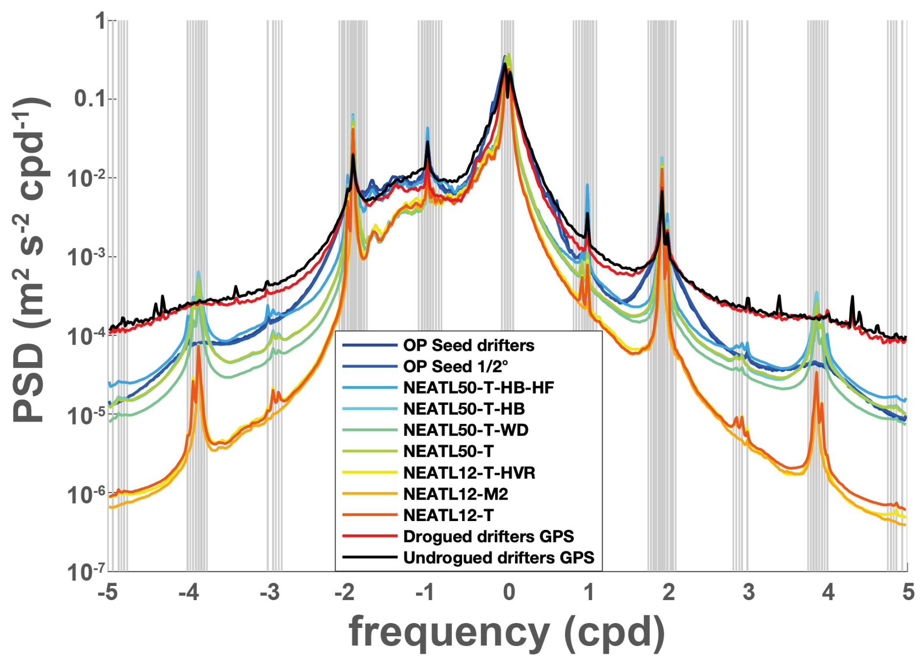
Figure 2 Rotary spectra of surface horizontal kinetic energy averaged over offshore regions for the NEATL domain between −5 and 5 cycles per day (cpd) from the HYCOM simulations, OceanParcels (OP) experiments and from surface drifters. Cyclonic and anticyclonic motions are assigned to positive and negative frequencies, respectively. The vertical gray lines indicate tidal frequencies in both positive and negative frequency domains from Arbic et al. (2022). Note the decimal logarithmic scale for the Power Spectrum Density (PSD).

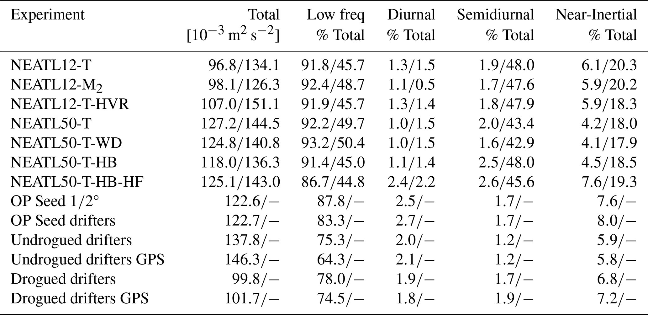
Table 2 Surface horizontal kinetic energy (SHKE) averaged over the NEATL domain for the seven HYCOM experiments, the OceanParcels (OP) experiments, and surface drifters. For both types of surface drifters (drogued and undrogued), two datasets are considered, one that includes GPS-tracked drifters only and one with all drifters (both Argos and GPS positioning systems). Presented below are the total SHKE, and percentage of the total SHKE stored in low-frequency ($>-\mathrm{0.5}$ and <0.5 cpd); diurnal frequency (±[0.9, 1.1] cpd); semidiurnal frequency (±[1.9, 2.1] cpd); and near-inertial frequency (±[0.9, 1.1]f cpd poleward of ±5° latitude) reservoirs (see Table S1 in the Supplement for absolute value of SHKE in each reservoirs). Each cell shows SHKEd/SHKEs where SHKEd and SHKEs represent SHKE values computed in waters deeper and shallower than 500 m, respectively. SHKEs are not provided for Lagrangian fields (i.e., OP and drifters) due to the low density of observations in these regions (Fig. 1).

The rotary spectra for the observed surface drifters, the OceanParcels numerical drifters, and the seven HYCOM simulations, computed and averaged over the NEATL offshore domain (depth greater than 500 m), are displayed in Fig. 2. The overall pattern is similar for all, with higher energy levels at low frequencies, forming a broad peak, and with kinetic energy decreasing as the absolute value of the frequency increases and with pronounced peaks at the tidal forcing frequencies. Within the ±2 cpd range, the spectra are not symmetric about zero frequency, with consistently more energy on the anticyclonic domain (assigned to negative frequencies in Fig. 2), reflecting the predominance of the anticyclonic near-inertial oscillations. All Eulerian estimates exhibit peaks at the tidal frequencies (gray lines in Fig. 2), with the exception of NEATL12-M₂, which is forced solely by the M₂ constituent and therefore lacks the other tidal peaks. The peaks in SHKE at higher frequencies are either absent or less marked in the Lagrangian datasets (i.e., observed and numerical drifters), in agreement with Arbic et al. (2022). The most notable difference among the datasets lies in the level of energy in the high-frequency internal gravity wave continuum (Garrett and Munk, 1975) with the highest values in the observed drifters datasets (drogued and undrogued) and the lowest in the coarse-resolution $\mathrm{1}/\mathrm{12}$° horizontal grid-spacing simulations. There is a significant increase of energy in the $\mathrm{1}/\mathrm{50}$° (Lagrangian and Eulerian) horizontal grid-spacing simulations, but they do not reach the level of the observations.

To obtain a quantitative measure of the differences, we also compute the domain-averaged surface SHKE and its distribution across different frequency bands for all datasets. In order to compare variations in energy distribution among datasets that do not have the same total SHKE, we express the energy in each frequency reservoir as a fraction of the total SHKE (Table 2).

As pointed out by Yu et al. (2019) and Arbic et al. (2022), most of the energy in the offshore domain waters (deeper than 500 m) is contained in the low-frequency band, representing 83 %–93 % of the total SHKE for the numerical simulations and 64 %–78 % for the drifters (Table 2). This is expected given that large- and mesoscale motions account for most of the oceanic kinetic energy (Wunsch and Stammer, 1995; Ferrari and Wunsch, 2009; Morrow and Le Traon, 2012). In contrast, the diurnal, semidiurnal and near-inertial narrower frequency intervals contain between one and two orders of magnitude less energy. Although their fractional contribution is small, high-frequency motions play an important role since they are the main pathways for energy transfer and mixing in the ocean interior (Wunsch and Ferrari, 2004; Müller et al., 2005).

When we extend the analysis of Yu et al. (2019) and Arbic et al. (2022) to waters shallower than 500 m, the results (Table 2) are markedly different, with the total SHKE being higher on average inshore than offshore and with the low-frequency band accounting for only 45 %–50 % of the total (Table 2), leaving considerably more energy associated with higher-frequency motions in inshore areas. In the diurnal band, the difference in the energy between offshore and inshore varies across configurations with no consistent pattern, but there is a striking difference in the semidiurnal and near-inertial bands. For the semidiurnal band, the continental shelf can contain up to 25 times more energy fraction than the deep ocean, while the near-inertial band shows a more moderate but still significant enhancement by a factor of 3 to 4 (Tables 2 and S1 in the Supplement). Tidal shoaling implies that, as water depth decreases, mass conservation requires higher barotropic velocities and hence larger SHKE of the barotropic tide, even if a portion of the barotropic energy is converted into internal tides (see demonstration of a tidal wave crossing a slope without reflection or friction in Pugh and Woodworth, 2014). However, shoaling should affect both the diurnal and semidiurnal bands similarly, which is not what we observe. In addition, in the NEATL domain, several shelf and marginal basins exhibit resonant behavior that selectively amplifies tidal components, depending on their geometry. Diurnal resonances occur in regions such as the Gulf of Mexico (e.g., Grace, 1932), whereas semidiurnal resonances are prominent in the Hudson Bay (e.g., Cummins et al., 2010), the North Sea (e.g., Jänicke et al., 2021), the English Channel and Irish Sea (e.g., Webb, 2013), and the Bay of Fundy–Gulf of Maine system (e.g., Garrett, 1972). Therefore, area-averaged diagnostics cannot fully explain the differences between offshore and inshore energy frequency decomposition. Assessing how numerical parameter choices affect the spatial distribution of SHKE requires first establishing a reliable observational reference (Sect. 4), before examining sensitivities through the experimental framework (Sect. 5).

4 Lagrangian spectral estimates of SHKE

Comparing model outputs to surface drifter observations requires accounting for the distortion in the low frequency and tidal variance introduced by the Lagrangian nature of drifter sampling. To this end, we compare rotary spectra from undrogued drifters with those from OP Seed Drifters, a subset of numerical particles advected in the NEATL50-T-HB-HF simulation and subsampled to replicate the number and spatial distribution of undrogued drifter segments. NEATL50-T-HB-HF is our “best” $\mathrm{1}/\mathrm{50}$° experiment (fine bathymetry and hourly winds) in the sense that it most closely matches observations in the globally averaged rotary spectra (Fig. 2). We then compare the same Lagrangian estimates to their Eulerian counterpart.

4.1 Observed versus numerical drifters

In Fig. 2, only the GPS-tracked drifters were used to minimize the noise (Yu et al., 2019). In contrast, all undrogued drifters are included in Fig. 3, as restricting the analysis to GPS-tracked drifters would lead to insufficient spatial coverage in parts of the domain (e.g., the equatorial South Atlantic; see Fig. S1 in the Supplement).

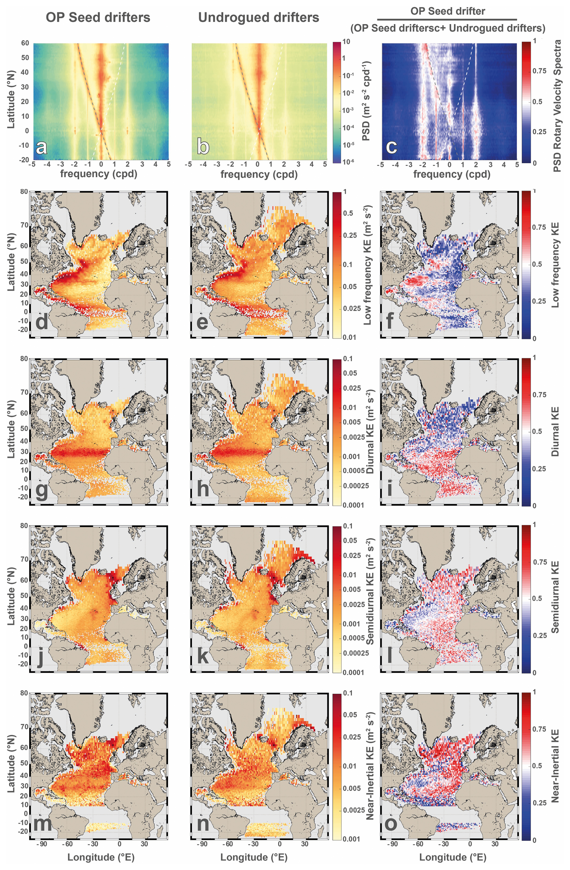
Figure 3 Comparison of OP Seed Drifters (first column) and undrogued surface drifters (second column), with a normalized ratio obtained by dividing the first column by the sum of the first and second columns (third column); a ratio of $\mathrm{1}/\mathrm{2}$ indicates equal energies. The first row (a–c) shows the zonally averaged rotary spectra in 1° latitude bins computed over the offshore domain (waters deeper than 500 m) in the NEATL domain; note the decimal logarithmic color scale for panels (a) and (b). The subsequent rows show maps of surface horizontal kinetic energy (SHKE) components over the NEATL domain: low-frequency ($>-\mathrm{0.5}$ and <0.5 cpd; second row (d–f)); diurnal (±[0.9, 1.1] cpd; third row (g–i)); semidiurnal (±[1.9, 2.1] cpd; fourth row (j–l)); and near-inertial (±[0.9, 1.1]f cpd restricted poleward of ±5° latitude; fifth row (m–o)). Note the decimal logarithmic color scale for all map panels.

The zonally averaged rotary spectra of OP Seed Drifters and undrogued drifters are shown in the first row of Fig. 3. Before contrasting the two datasets, we note that, near 30° N, the inertial frequency (grey dashed line) coincides with the diurnal tidal frequency (±1 cpd), making it difficult to disentangle their respective contributions. This latitude corresponds to the diurnal critical latitude (e.g., 27.6° for O₁ and 30° for K₁; Robertson, 2001), defined as the latitude where the inertial frequency equals the tidal frequency (e.g., Middleton and Denniss, 1993; Robertson, 2001). According to linear internal wave theory, it marks the poleward limit of wave propagation so, poleward of 30°, diurnal internal tides become evanescent. The critical latitude for the semidiurnal (±2 cpd) band is much higher, around 75° (e.g., 74.5° for M₂ and 85.7° for S₂; Furevik and Foldvik, 1996; Robertson, 2001), allowing semidiurnal internal waves to propagate across most of the global ocean.

The pattern of the zonally averaged PSD of rotary spectra is similar between the observed and numerical drifters (Fig. 3a and b). However, the observed drifters show more energy in the high-frequency band, while the semidiurnal and diurnal peaks are, at most latitudes, more pronounced in the NEATL50-T-HB-HF numerical drifters. As discussed by Arbic et al. (2022), this high-frequency content in the observed drifters may originate from the drifter tracking system (Yu et al., 2019) and/or from artifacts in the estimation of drifter positions and velocities (Elipot et al., 2016). Overall, the numerical drifters contain less total SHKE than the observed undrogued surface drifters (Table 2). Yet, they contribute to a significantly higher fraction to the low-frequency band, storing 83.3 % of the total SHKE (87.8 % of OP Seed $\mathrm{1}/\mathrm{2}$°). In comparison, the undrogued drifters store 75.3 % in the low-frequency band (64.3 % for GPS-tracked drifters). In absolute and relative terms, the numerical particles exhibit more energy than observed in the semidiurnal and near-inertial bands.

The normalized ratio (right column in Fig. 3) reveals clear spatial contrasts between the numerical simulation and the observations. Indeed, there is a striking bipolar pattern in the diurnal band (Fig. 3i) that is more pronounced in the observations with higher SHKE poleward of the diurnal critical latitude and less equatorward of it. This observed poleward diurnal energy is consistent with Arbic et al. (2022), who reported that diurnal motions are driven not only by tides, but also by the day/night solar heating cycle. At low frequencies, the model indicates higher SHKE in energetic regions such as the Gulf of Mexico and the Gulf Stream whereas the surface drifters show the opposite (Fig. 3f). In the semidiurnal and near-inertial bands, the pattern reverses, with observations exhibiting higher SHKE in these energetic regions, whereas the model distributes energy more broadly (Fig. 3l and o). The effect of temporal coverage mismatch, resulting from the difference between the 30-year observational record and the single-year OP drifter simulation, is also weakly discernible in the near-inertial band. Indeed, the two narrow bands of enhanced near-inertial energy between 20 and 30° N in panel (m) of Fig. 3 for the 1-year numerical OceanParcels simulation correspond to the tracks of Hurricanes Fabian and Kate of the 2003 season (the atmospheric forcing year of the simulation), a feature that is even more apparent in the Eulerian fields (Fig. 4m).

Overall, the undrogued surface drifter data contains more total SHKE than NEATL50-T-HB-HF numerical particles, with the model over-representing the fraction of energy in the near-inertial and tidal reservoirs. Regionally, the sign of the model–observation discrepancy depends on the frequency band. At low frequencies, the modeled energy exceeds the observed one in the western boundary currents, whereas the reverse holds elsewhere. By contrast, in the semidiurnal and near-inertial bands, the observed energy exceeds the modeled one in these same energetic regions. The largest discrepancy is in the diurnal band. South of the diurnal critical latitude, where internal tides radiate freely, the modeled diurnal energy exceeds the observed one while observations exceed the modeled one poleward, where only non-tidal mechanisms can sustain diurnal energy. Whether these discrepancies reflect genuine model biases or arise partly from the Lagrangian sampling framework is examined in the following subsection.

4.2 Lagrangian versus Eulerian sampling

The previous subsection established the differences between OP Seed Drifters and undrogued surface drifters. The effect of drifter sampling density on the 60 d segments and corresponding spectra was found to be small and spatially incoherent (see comparison between the high density OP Seed $\mathrm{1}/\mathrm{2}$° and subsampled OP Seed Drifters in Fig. S2 and Sect S3 of the Supplement). Restricting the undrogued drifter statistics to the OP Seed Drifters footprint (between 25° S and 65° N, not shown) yields nearly identical frequency distributions (to within 0.1 percentage points), with only a modest increase of total SHKE from 137.8 to $\mathrm{144.4}\times {\mathrm{10}}^{-\mathrm{3}}$ m² s⁻². This confirms that the spatial coverage of the OP experiments is not the main driver of the frequency-distribution mismatch between the model and the observations.

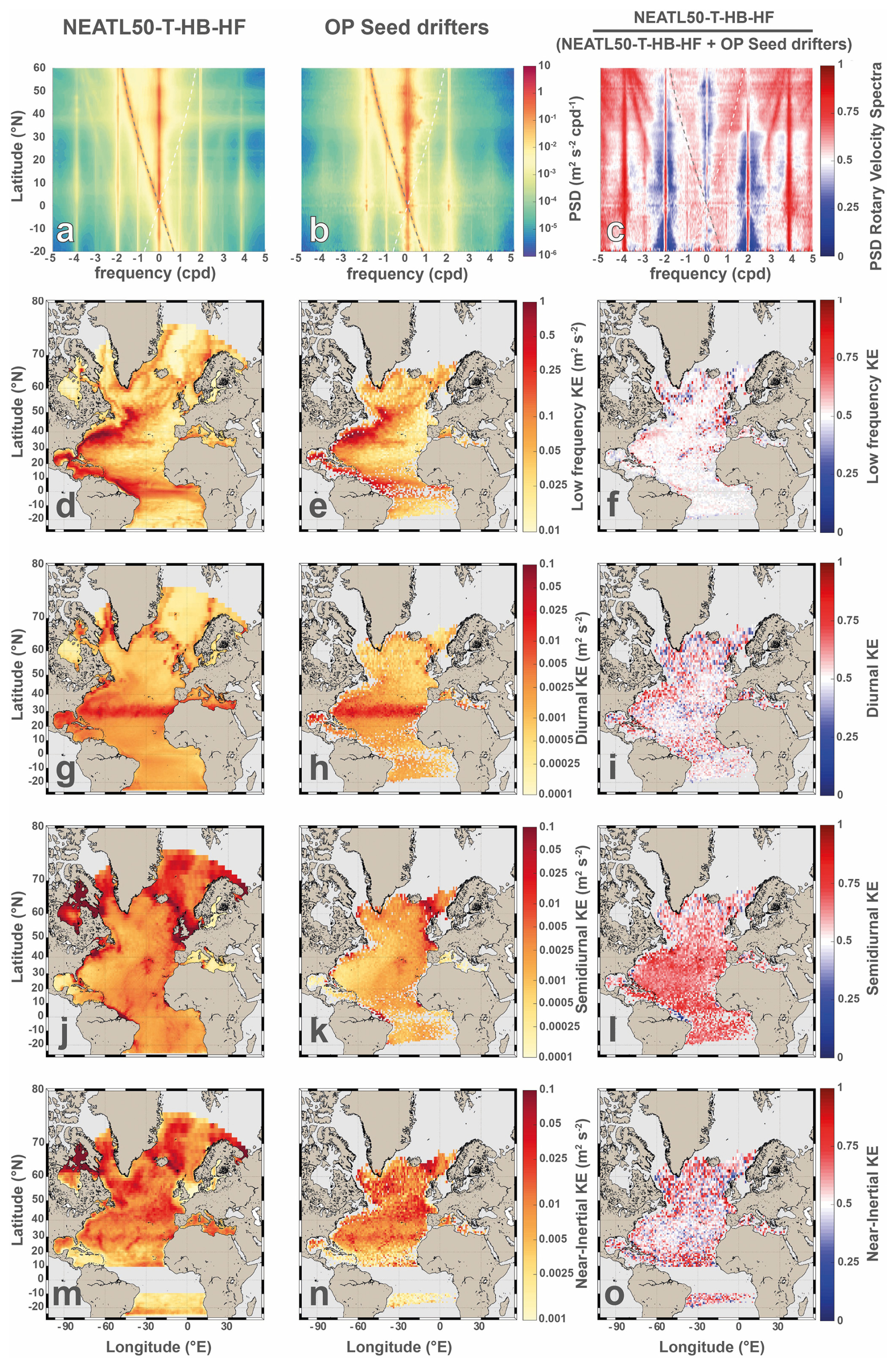
Figure 4 Comparison of NEATL50-T-HB-HF (first column) and OP Seed Drifters (second column), with a normalized ratio obtained by dividing the first column by the sum of the first and second columns (third column); a ratio of 1/2 indicates equal energies. The first row (a–c) shows the zonally averaged rotary spectra in 1°  latitude bins computed over the offshore domain (waters deeper than 500 m) in the NEATL domain; note the decimal logarithmic color scale for panels (a) and (b). The subsequent rows show maps of surface horizontal kinetic energy (SHKE) components over the NEATL domain: low-frequency ($>-\mathrm{0.5}$ and < 0.5 cpd; second row (d–f)); diurnal (±[0.9, 1.1] cpd; third row (g–i)); semidiurnal (±[1.9, 2.1] cpd; fourth row (j–l)); and near-inertial (±[0.9, 1.1]f cpd restricted poleward of ±5° latitude; fifth row (m–o)). Note the decimal logarithmic color scale for all map panels.

The zonally averaged PSD is overall similar between the native Eulerian fields and OP Seed Drifters (Fig. 4a and b), but the tidal peaks are broader and increasingly indiscernible at higher frequencies in the Lagrangian spectra (e.g., the ±4 cpd peaks are barely discernible in the Lagrangian but prominent in the Eulerian). This spectral broadening redistributes energy away from peak centers toward neighboring frequencies, as shown by the ratio in Fig. 4c and consistent with observations from earlier work (Davis, 1983; Middleton, 1985; Zaron and Elipot, 2021; Caspar-Cohen et al., 2022, 2025; Zhang et al., 2024). Above approximately ±2.5 cpd, the Eulerian spectrum shows clear mirror images of the inertial ridge at $-f\pm \mathrm{1}$ cpd that appear as a surplus of Eulerian over Lagrangian energy (Fig. 4c), while these features are barely discernible in the OP Seed Drifter (Fig. 4b) and undrogued drifters spectra (Fig. 3b). Their presence in our Eulerian fields corroborates the interpretation by Arbic et al. (2022), namely that such mirror images, previously identified in global surface drifters (Elipot et al., 2016) and in both Eulerian and Lagrangian global tide-resolving simulations (Zhang et al., 2024), reflect genuine oceanic processes. However, the attenuation of these mirror images in the Lagrangian spectrum suggests that the undrogued drifter sampling in the NEATL domain, although adequate for the frequency bands considered here, may under-resolve these weaker high-frequency features. Domain-averaged energy in specific frequency reservoirs (Tables 2 and S1) shows that the different velocities (Lagrangian vs. Eulerian) have minimal impact on total SHKE and in low, diurnal, and near-inertial bands. However, significant deviations occur in the semidiurnal frequency band with Eulerian velocities containing up to 50 % more energy than Lagrangian velocities. The SHKE maps (Fig. 4) confirm comparable levels of energy for low, diurnal and near-inertial frequencies. In the semidiurnal band, OP Seed Drifters show less energy over most of the domain with a notable exception at the Amazon shelf (Fig. 4j), a well-known hotspot of semidiurnal barotropic and internal tides (e.g., Gabioux et al., 2005; Beardsley et al., 1995; Tchilibou et al., 2022) where Lagrangian particles are advected across strong velocity gradients at each tidal cycle, likely amplifying the apparent tidal energy relative to Eulerian estimates.

The comparison of Lagrangian and Eulerian estimates (Fig. 4) shows that the differences observed between OP Seed Drifters and undrogued surface drifters (Fig. 3) cannot be attributed to the Lagrangian sampling alone. In particular, the lower (higher) energy poleward (equatorward) of 30° N and the deficit of high frequency energies in the model relative to observations are not visible when comparing OP Seed Drifters to the Eulerian fields, confirming that these are genuine dataset differences rather than an outcome of the Lagrangian sampling. Note that the high-frequency deficit in the simulations could partially be the result of drifter tracking and position-estimation artifacts (Elipot et al., 2016; Yu et al., 2019; Arbic et al., 2022) or wind slippage (Niiler and Paduan, 1995; Arbic et al., 2022) instead of real oceanic motions. Similarly, the higher observed SHKE in strong low-frequency flow, seen in the near-inertial and semidiurnal bands of the observation compared to the numerical drifters, is not recovered as a Lagrangian/Eulerian difference in our twin-simulation experiments. This contrasts with Zhang et al. (2024), who reported a Lagrangian underestimation of low-frequency and diurnal KE relative to the Eulerian field in regions of strong low-frequency flow. This apparent disagreement may be a consequence of a difference in experimental design as their analysis relied on a very large ensemble of particles distributed throughout the same simulation, providing the statistical power to isolate small Lagrangian sampling effects on energetic mesoscale regions. As in Zhang et al. (2024) and Caspar-Cohen et al. (2025), the main effect of the Lagrangian sampling is the spectral broadening of tidal peaks which has a negligible impact on the frequency distribution of low, diurnal and near-inertial bands (Table 2). In the semidiurnal band, however, the broadening is more pronounced, with the Eulerian fields storing 2.6 % of total SHKE compared to 1.7 % in the Lagrangian experiment, implying that part of any semidiurnal discrepancy between observations and Eulerian model output may reflect the Lagrangian/Eulerian framework itself.

5 Impact of model configuration and parameter choices on SHKE

Overall, the fact that the numerical simulations have less total SHKE than the observed undrogued drifters and that all also allocate a larger fraction of that energy to low frequencies (Table 2) is not a consequence of the drifters' Lagrangian sampling. There are, however, large differences in the other frequency bands among the numerical sensitivity experiments when compared to the observations and those are not uniform (Table 2). To quantify these differences, we analyze in detail the controlled series of sensitivity experiments where a single model parameter at a time to document the influence of resolution, tidal content, wind-forcing frequency, bathymetry, and wave drag, respectively.

5.1 Number of tidal components

NEATL12-T and NEATL12-M₂ differ only in the number of tidal components forcing the model (eight largest tidal constituents and M₂ only, respectively). Their zonally averaged rotary spectra are broadly similar (Fig. 5a–c), but NEATL12-T has greater energy in the vicinity of the tidal peaks. This is particularly evident in the normalized ratio (Fig. 5c), except at the exact position of the M₂ frequency (around ±2 cpd) and its pure second harmonic (around ±4 cpd, see Ray (2007)), where the tidal peak of NEATL12-M₂ is comparable to that of NEATL12-T (i.e., normalized ratio near 0.5 in Fig. 5c). Globally, the total SHKE remains essentially unchanged between the two runs (Table 2), with a slight decrease offshore and a more notable increase on the shelf in NEATL12-T. When fewer constituents are retained, the low-frequency component contains a slightly larger fraction of the total SHKE (i.e., 91.8 % offshore and 45.7 % inshore in NEATL12-T against 92.4 % offshore and 48.7 % inshore in NEATL12-M₂) while the near-inertial bands contain a slightly smaller fraction. There is also an increase in the semidiurnal fraction of total SHKE in NEATL12-T compared to NEATL12-M₂ but the diurnal band concentrates the strongest contrast, with NEATL12-T more energetic both offshore and inshore but the largest differences are on the coast (a factor of three in both absolute and relative terms).

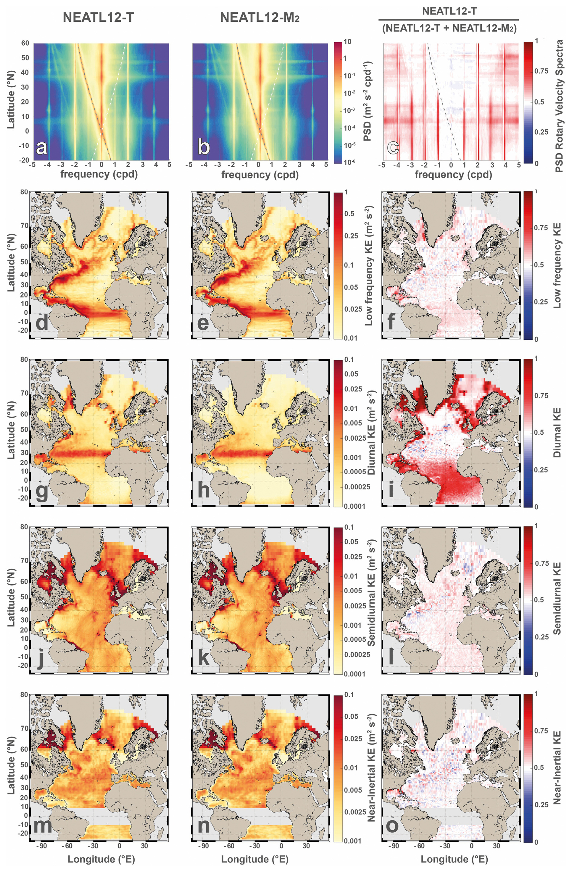
Figure 5 Comparison of NEATL12-T (first column) and NEATL12-M₂ (second column), with a normalized ratio obtained by dividing the first column by the sum of the first and second columns (third column); a ratio of $\mathrm{1}/\mathrm{2}$ indicates equal energies. The first row (a–c) shows the zonally averaged rotary spectra in 1°  latitude bins computed over the offshore domain (waters deeper than 500 m) in the NEATL domain; note the decimal logarithmic color scale for panels (a) and (b). The subsequent rows show maps of surface horizontal kinetic energy (SHKE) components over the NEATL domain: low-frequency ($>-\mathrm{0.5}$ and < 0.5 cpd; second row (d–f)); diurnal (±[0.9, 1.1] cpd; third row (g–i)); semidiurnal (±[1.9, 2.1] cpd; fourth row (j–l)); and near-inertial (±[0.9, 1.1]f cpd restricted poleward of ±5° latitude; fifth row (m–o)). Note the decimal logarithmic color scale for all map panels.

Regionally (Fig. 5), no clear contrast between the two experiments emerges in the low-frequency, semidiurnal, and near-inertial bands with NEATL12-T being slightly more energetic in most of the domain. The diurnal band tells a different story with a clear separation at 30° N. Poleward of 30° N the two experiments are comparable offshore, whereas equatorward of 30° N NEATL12-T is significantly more energetic. On the shelves, the NEATL12-T excess of diurnal SHKE is present at all latitudes, including north of 30° N.

Overall, adding more tidal components increases, as expected, the energy at the added frequencies, with the largest increase on the continental shelves where, through tidal shoaling, the barotropic tidal amplitudes are largest (Pugh and Woodworth, 2014). In the semidiurnal band, the slightly smaller fraction found in NEATL12-M₂ might reflect the absence of S₂, N₂, and K₂ constituents, which together contribute a non-negligible share of the global semidiurnal signal. Offshore and poleward of 30° N, the diurnal signal is nearly identical in both runs, highlighting that, as discussed by Arbic et al. (2022), a large fraction of the diurnal flow is non-tidal. Possible sources for this non-tidal diurnal SHKE are the wind variability (Dai and Deser, 1999; Savazzi et al., 2022; Dai, 2023) (further discussed in Section 5.6) and/or aliasing of mesoscale variability (Shriver et al., 2012; Buijsman et al., 2025). By contrast, the diurnal energy is substantially larger near the equator and on the shelves in NEATL12-T than in NEATL12-M₂, showing that the diurnal tidal constituents (K₁, O₁, P₁, Q₁) dominate the local diurnal variability in these regions.

5.2 Horizontal resolution

NEATL50-T and NEATL12-T differ only in horizontal resolution ($\mathrm{1}/\mathrm{50}$° and $\mathrm{1}/\mathrm{12}$°, respectively). The zonally averaged rotary spectra (Fig. 6a–c) show that NEATL50-T is significantly more energetic at nearly all frequencies (see Fig. 2 of Chassignet and Xu (2017) for a comparison of the time evolution of the domain-averaged total 3D kinetic energy where $\mathrm{1}/\mathrm{50}$° has approximately 70 % more energy than $\mathrm{1}/\mathrm{12}$°). This is confirmed by examining the ratio in Fig. 6c and particularly true for frequencies whose absolute value exceeds 2 cpd. However, NEATL50-T and NEATL12-T have close levels of energy at tidal peaks close to ±2 cpd. The only exception to the rule that higher resolution yields higher energy is that NEATL12-T has more energy in the −[0.9, 1.1]f cpd frequency band, which corresponds to near-inertial motions in the northern hemisphere but to the cyclonic side of the spectrum in the southern hemisphere. Table 2 quantifies that the SHKE in the deep ocean increases by around one-third when the horizontal resolution increases from $\mathrm{1}/\mathrm{12}$ to $\mathrm{1}/\mathrm{50}$° horizontal grid-spacing; however, the differences are less pronounced on the continental shelf. The excess of energy is, roughly, well distributed across the different reservoirs, as the percentage of the total SHKE stored in each compartment is comparable between the two experiments. In detail, the most noticeable difference occurs in the deep ocean where the percentage of total SHKE stored in the near-inertial band decreases by one-third (from 6 % to 4 %) as the resolution increases.

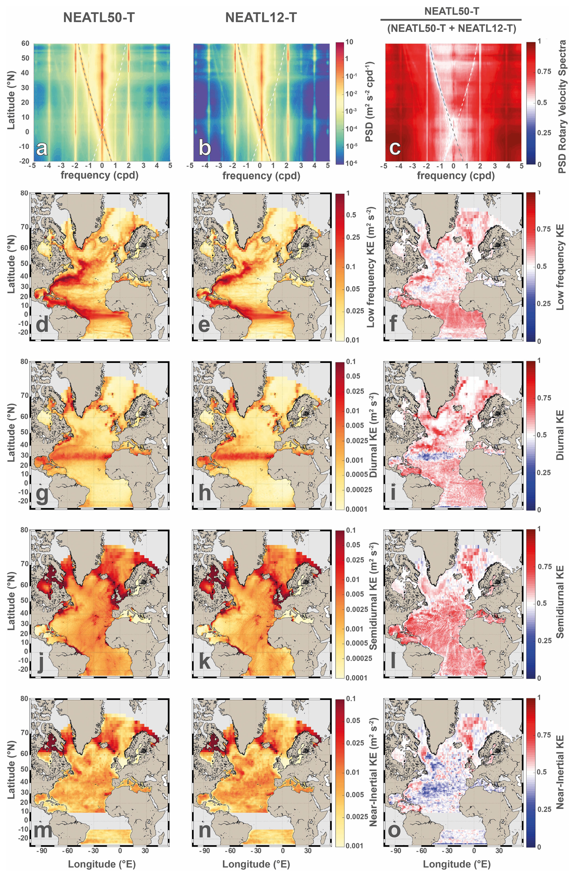
Figure 6 Comparison of NEATL50-T (first column) and NEATL12-T (second column), with a normalized ratio obtained by dividing the first column by the sum of the first and second columns (third column); a ratio of $\mathrm{1}/\mathrm{2}$ indicates equal energies. The first row (a–c) shows the zonally averaged rotary spectra in 1° latitude bins computed over the offshore domain (waters deeper than 500 m) in the NEATL domain; note the decimal logarithmic color scale for panels (a) and (b). The subsequent rows show maps of surface horizontal kinetic energy (SHKE) components over the NEATL domain: low-frequency ($>-\mathrm{0.5}$ and < 0.5 cpd; second row (d–f)); diurnal (±[0.9, 1.1] cpd; third row (g–i)); semidiurnal (±[1.9, 2.1] cpd; fourth row (j–l)); and near-inertial (±[0.9, 1.1]f cpd restricted poleward of ±5° latitude; fifth row (m–o)). Note the decimal logarithmic color scale for all map panels.

Over most of the domain (Fig. 6), the NEATL50-T simulation has significantly more energy than NEATL12-T at low, diurnal, and semidiurnal frequencies. However, the opposite is true for the near-inertial frequency. By contrast, near 30° latitude in the diurnal band, NEATL12-T has more energy than NEATL50-T, but this corresponds to the latitude where energy stored in the near-inertial band overlaps with that in the diurnal band (Arbic et al., 2022; Raja et al., 2022).

Overall, increasing the horizontal resolution leads to a substantial increase in total SHKE across most of the energy spectrum, consistent with previous studies. Chassignet et al. (2020) showed that high horizontal-resolution simulations have much higher values of kinetic energy for low frequency motions compared to low-resolution simulations. For tidal frequencies, Buijsman et al. (2020) found that increasing the horizontal resolution in realistic HYCOM simulations from 8 to 4 km increased the semidiurnal barotropic-to-baroclinic tidal conversion by half, and more baroclinic modes were resolved. Nelson et al. (2020) also found that decreasing the horizontal grid spacing leads to more realistic internal wave frequency spectra. The increase in horizontal resolution also leads to a better representation of the submesoscale field, and increases wave-mean and wave–wave interactions, explaining the filling of the high-frequency continuum between the tidal peaks (Garrett and Munk, 1975) in the $\mathrm{1}/\mathrm{50}$° simulations when compared to the $\mathrm{1}/\mathrm{12}$° simulations (Figs. 2 and 6c). There are two exceptions to this overall increase in SHKE. First, the semidiurnal fraction of the inshore SHKE decreases from 48.0 % to 43.4 % while the offshore fraction barely changes (1.9 % to 2.0 %; Table 2). A possible explanation is that over continental shelves, where the semidiurnal signal is predominantly barotropic and a large fraction of the global M₂ energy is dissipated (Egbert and Ray, 2001), enhanced barotropic-to-baroclinic conversion (Niwa and Hibiya, 2011; Buijsman et al., 2020) redistributes energy away from the barotropic tide, while the generated internal tide radiates seaward and is not retained locally. Yu et al. (2019) also suggested that insufficient horizontal resolution could enhance the semidiurnal peak by inhibiting scattering of tidal energy into the wave continuum (Müller et al., 2015; Shriver et al., 2012). Second, the near-inertial band is weaker on average at the higher horizontal resolution. One possible interpretation could be a more efficient vertical transport of near-inertial kinetic energy into the ocean interior through the resolved mesoscale and submesoscale fields in the $\mathrm{1}/\mathrm{50}$° simulation (e.g., Kunze, 1985; Thomas et al., 2020; Lu et al., 2023). However, the spatial pattern in near inertial SHKE reduction does not straightforwardly support this view, since the reduction is not systematically concentrated in the most energetic regions of the domain (Fig. 6d), where mesoscale activity is strongest, but rather appears in the basin interior.

5.3 Vertical resolution

NEATL12-T-HVR and NEATL12-T differ only in vertical resolution (96 and 32 isopycnal layers, respectively). The zonally averaged rotary spectra (Fig. 7a–b) show no clear differences in total SHKE, tidal peaks or harmonics. However, the normalized ratio indicates slightly more energy in the northern high latitudes with more vertical levels and less energy in the low latitudes. As seen in Table 2, increasing the vertical resolution from 32 to 96 levels results in approximately a 10 % to 15 % increase in total SHKE, with the increase being higher over the continental shelf. Because the fraction of total SHKE in each band is largely unchanged (Table 2), this additional energy is distributed broadly across the frequency domain. The most remarkable difference seen here is that, by increasing the vertical resolution, around 2 % less of the total SHKE is stored in the near-inertial frequencies over the continental shelf.

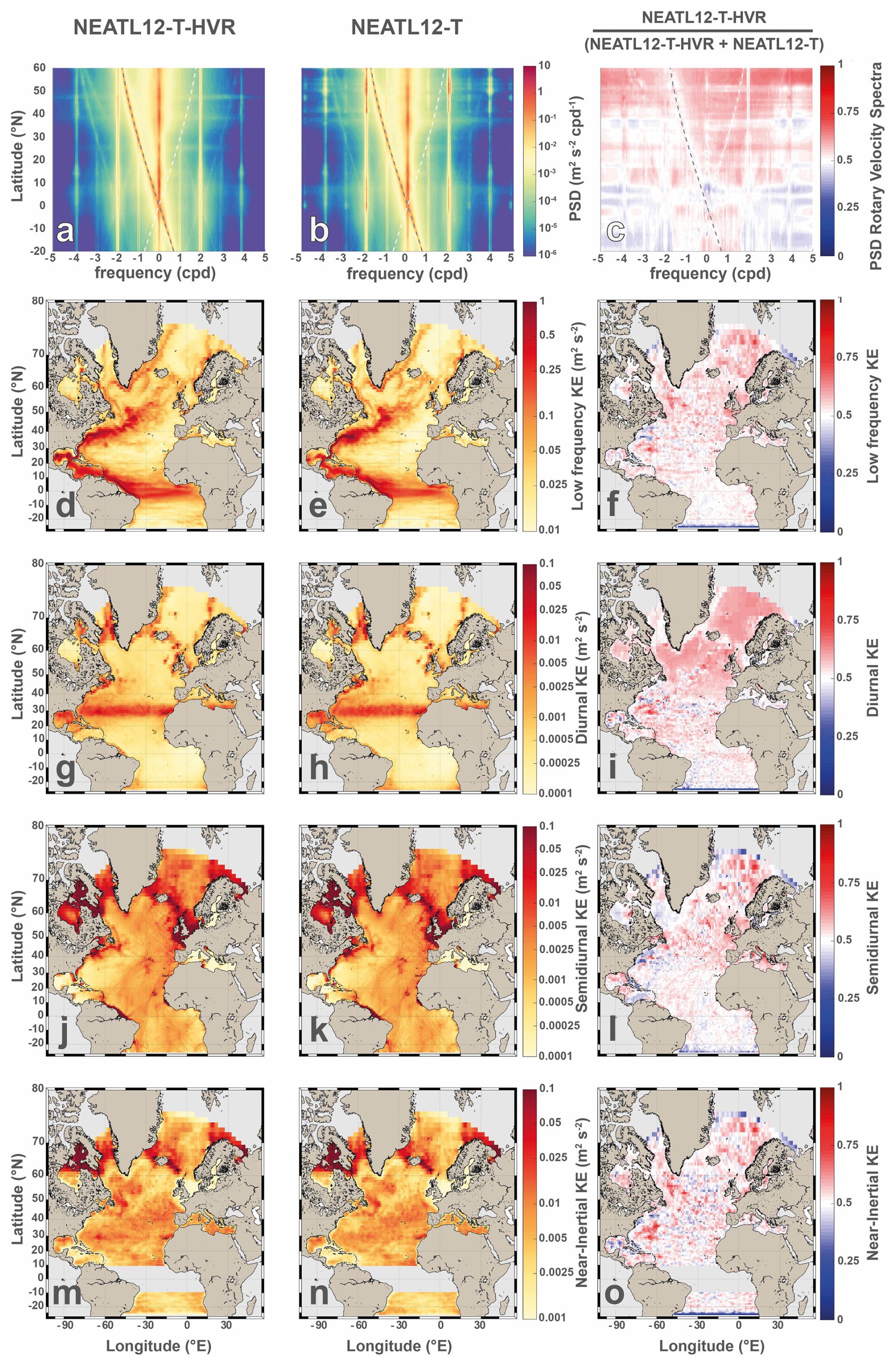
Figure 7 Comparison of NEATL12-T-HVR (first column) and NEATL12-T (second column), with a normalized ratio obtained by dividing the first column by the sum of the first and second columns (third column); a ratio of $\mathrm{1}/\mathrm{2}$ indicates equal energies. The first row (a–c) shows the zonally averaged rotary spectra in 1°  latitude bins computed over the offshore domain (waters deeper than 500 m) in the NEATL domain; note the decimal logarithmic color scale for panels (a) and (b). The subsequent rows show maps of surface horizontal kinetic energy (SHKE) components over the NEATL domain: low-frequency ($>-\mathrm{0.5}$ and < 0.5 cpd; second row (d–f)); diurnal (±[0.9, 1.1] cpd; third row (g–i)); semidiurnal (±[1.9, 2.1] cpd; fourth row (j–l)); and near-inertial (±[0.9, 1.1]f cpd restricted poleward of ±5° latitude; fifth row (m–o)). Note the decimal logarithmic color scale for all map panels.

The maps in Fig. 7 confirm the domain-averaged picture. Surface kinetic energy increases slightly across most regions and frequency bands when vertical resolution is refined, with no strong spatial pattern. The main exception lies offshore north of 40° N, where the increase appears spatially uniform in the diurnal band. This signal reflects the general increase of the total SHKE, which stands out visually in this otherwise low-energy region, rather than a diurnal-specific enhancement. Another exception regards regions of intense mesoscale activity, with elevated low-frequency energy in the corridors of North Brazil Current rings (Fratantoni and Glickson, 2002), Gulf of Mexico Loop Current eddies (Leben, 2005), and Gulf Stream meanders/rings, largely masked by the high background energy in the ratio panel (Fig. 7f), but evident when comparing the pathways in panels (d) and (e).

Overall, vertical refinement increases the total SHKE, distributed broadly across the frequency domain (see also Fig. 2), with a coherent enhancement at high latitudes. This is consistent with various studies that show that tidal energetics vary with the number of vertical layers provided that horizontal grid spacing is not the limiting factor. Nelson et al. (2020) showed that the modeled internal wave frequency spectra are improved with increased vertical resolution only when the horizontal resolution is also increased. In an idealized $\mathrm{1}/\mathrm{100}$° HYCOM configuration forced solely by semidiurnal tides, Hiron et al. (2025) found that increasing the number of isopycnal layers increases tidal-induced vertical velocities and available potential energy, while tidal kinetic energy remains largely unchanged. The energetics increase up to 48 layers and change little thereafter. Here, at $\mathrm{1}/\mathrm{12}$° horizontal grid-spacing, the tidal SHKE changes only weakly between 32 and 96 layers, and the tidal SHKE fraction even decreases slightly, suggesting that the horizontal grid-spacing is the limiting factor in our configuration. The dominant effect of vertical refinement is therefore an increase of low-frequency SHKE, also visible in total KE (not shown), in the already energetic meso- and large-scale flow regions, consistent with the primary role of the vertical grid in resolving horizontal flows via improved representation of their baroclinic structure (Stewart et al., 2017; Xu et al., 2023).

5.4 Impact of internal wave drag

NEATL50-T-WD and NEATL50-T differ only in the inclusion of internal wave drag (Jayne and St. Laurent, 2001) in NEATL50-T-WD. The zonally averaged rotary spectra (Fig. 8) show that the inclusion of wave drag reduces energy across the majority of the frequency domain. The reduction is less pronounced at frequencies below the near-inertial band, where it becomes almost negligible. Table 2 confirms that the inclusion of wave drag leads to a slight decrease in energy across all the frequency bands analyzed. The most pronounced impact is in the semidiurnal band, where the fraction of total SHKE drops by about 0.4 %–0.5 % both inshore (from 43.4 % to 42.9 %) and offshore (from 2.0 % to 1.6 %). While this represents a small relative change inshore, offshore it corresponds to a relative reduction of about $\mathrm{1}/\mathrm{5}$.

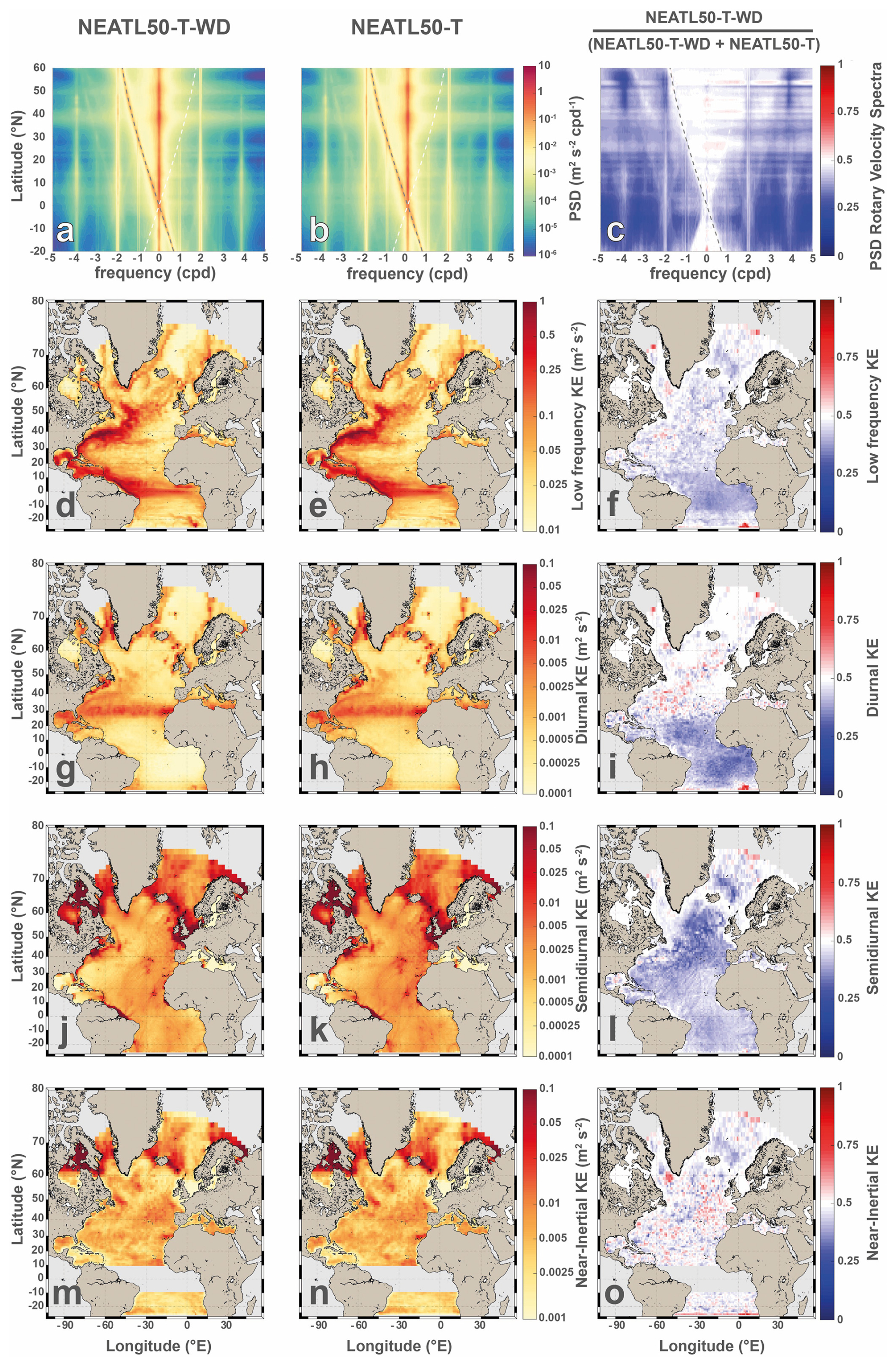
Figure 8 Comparison of NEATL50-T-WD (first column) and NEATL50-T (second column), with a normalized ratio obtained by dividing the first column by the sum of the first and second columns (third column); a ratio of $\mathrm{1}/\mathrm{2}$ indicates equal energies. The first row (a–c) shows the zonally averaged rotary spectra in 1°  latitude bins computed over the offshore domain (waters deeper than 500 m) in the NEATL domain; note the decimal logarithmic color scale for panels (a) and (b). The subsequent rows show maps of surface horizontal kinetic energy (SHKE) components over the NEATL domain: low-frequency ($>-\mathrm{0.5}$ and < 0.5 cpd; second row (d–f)); diurnal (±[0.9, 1.1] cpd; third row (g–i)); semidiurnal (±[1.9, 2.1] cpd; fourth row (j–l)); and near-inertial (±[0.9, 1.1]f cpd restricted poleward of ±5° latitude; fifth row (m–o)). Note the decimal logarithmic color scale for all map panels.

The SHKE maps (Fig. 8) confirm that incorporating wave drag leads to an overall reduction in surface SHKE across the frequency bands studied. In the low-frequency band, a clear reduction is visible in the tropical band equatorward of around ±15° (Fig. 8d–f). In the diurnal band, the reduction is most apparent equatorward of 30° N, while no clear signal emerges poleward of this latitude. In contrast, the decline in semidiurnal energy is more pronounced in the deep ocean at nearly all latitudes, with the exception of the western boundary current pathway from the Gulf of Mexico into the Gulf Stream (Fig. 8j–l). Finally, in the near-inertial band, no clear signal emerges.

Overall, the inclusion of wave drag reduces the energy in each frequency band over the latitudes where the corresponding motions can propagate, that is, equatorward of about ±15° for the low-frequency band (below ± 0.5 cpd), ±30° for the diurnal band, and across nearly the entire domain for the semidiurnal band, except along the western boundary current pathway. By construction, wave drag dissipates propagating tides, which explains the absence of a clear difference poleward of these critical latitudes, where the motions become evanescent. Yu et al. (2019) reported that the MITgcm tends to overestimate semidiurnal SHKE compared to surface drifters and, following Arbic et al. (2010) and Ansong et al. (2015), attributed this bias partly to the absence of topographic internal wave drag in the MITgcm simulations. Our results support this interpretation, with lower semidiurnal energy when wave drag is included.

5.5 Bathymetry resolution

NEATL50-T-HB and NEATL50-T differ only in bathymetric resolution, with NEATL50-T-HB using a native $\mathrm{1}/\mathrm{50}$° bathymetry rather than the $\mathrm{1}/\mathrm{12}$° product interpolated onto the $\mathrm{1}/\mathrm{50}$° grid (Chassignet et al., 2023). Overall, the higher-resolution bathymetry reduces the SHKE across most of the frequency domain (see Fig. 9a–c and Table 2). There are, however, notable exceptions in the semidiurnal and higher-frequency tidal peaks and in the latitudinal band between 20° N and 30° N, where the SHKE is higher in the high-resolution bathymetry simulation. The low-frequency fraction of SHKE is only marginally reduced (from 92.2 % to 91.4 %), whereas in shallow regions it drops more noticeably, from 49.7 % to 45.0 % (Table 2). There are minimal changes in the diurnal and near-inertial components, but enhancing the bathymetry resolution leads to increased energy in the semidiurnal frequency band. The percentage of KE contained in the semidiurnal band increased from 43.4 % to 48.0 % in the shelf domain, and from 2.0 % to 2.5 % in the offshore domain when high-resolution bathymetry was used.

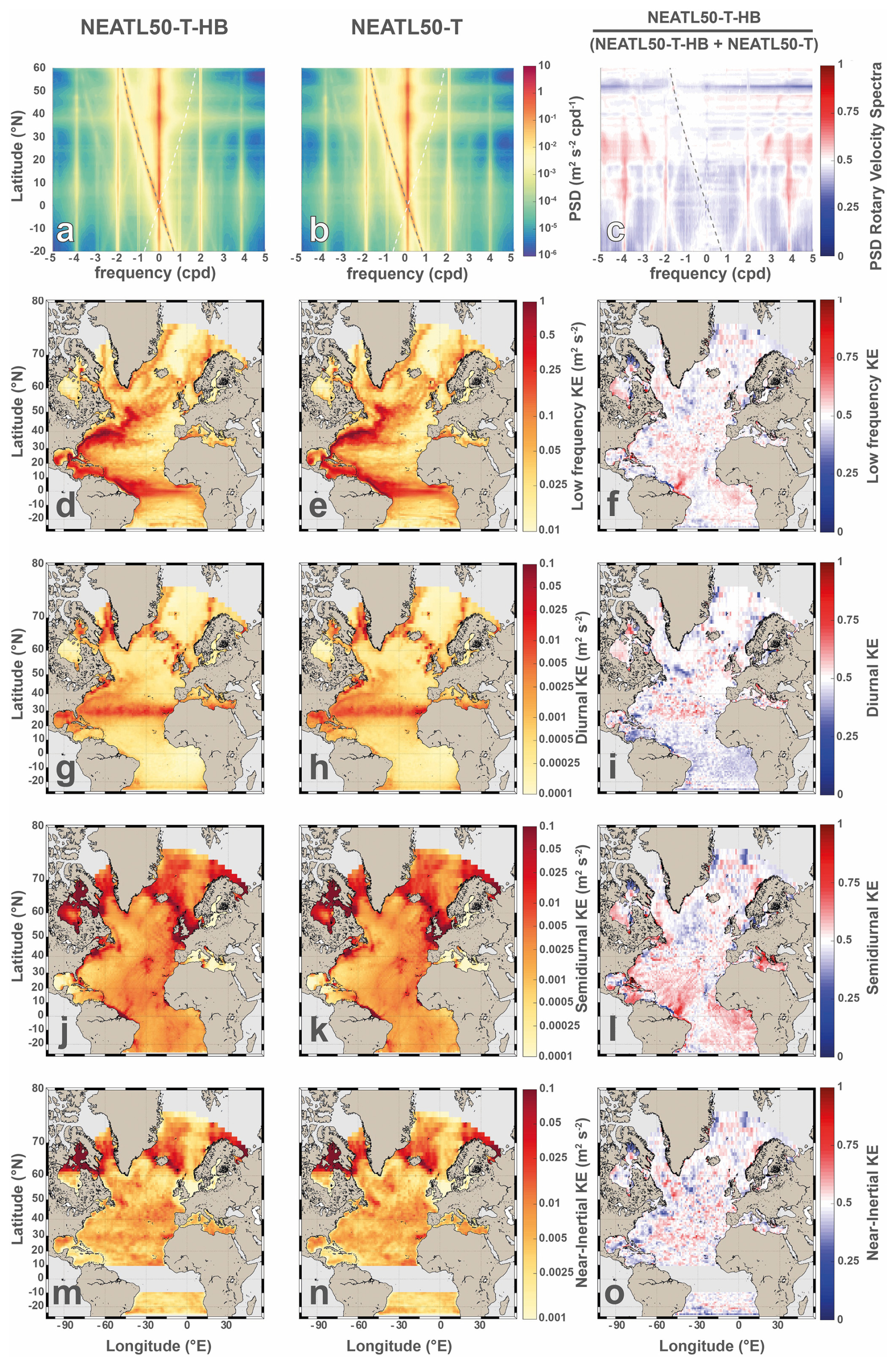
Figure 9 Comparison of NEATL50-T-HB (first column) and NEATL50-T (second column), with a normalized ratio obtained by dividing the first column by the sum of the first and second columns (third column); a ratio of $\mathrm{1}/\mathrm{2}$ indicates equal energies. The first row (a–c) shows the zonally averaged rotary spectra in 1°  latitude bins computed over the offshore domain (waters deeper than 500 m) in the NEATL domain; note the decimal logarithmic color scale for panels (a) and (b). The subsequent rows show maps of surface horizontal kinetic energy (SHKE) components over the NEATL domain: low-frequency ($>-\mathrm{0.5}$ and < 0.5 cpd; second row (d–f)); diurnal (±[0.9, 1.1] cpd; third row (g–i)); semidiurnal (±[1.9, 2.1] cpd; fourth row (j–l)); and near-inertial (±[0.9, 1.1]f cpd restricted poleward of ±5° latitude; fifth row (m–o)). Note the decimal logarithmic color scale for all map panels.

The SHKE maps (Fig. 9) do not show clear regional differences in the low-frequency and near-inertial bands. A noteworthy exception is the enhancement (diminution) of low-frequency SHKE below (above) the equator off the the Amazon shelf (Fig. 9f). In the diurnal frequency bandWith, there is a reduction of energy in the higher-resolution bathymetry experiment, with the exception of the 30° N latitude and a few specific regions such as the Adriatic Sea. By contrast, in the semidiurnal band, the increase in bathymetry resolution increases the surface SHKE, with a few exceptions, mainly at high latitudes. There is also a clear increase in the SHKE associated with semidiurnal internal tides in the Amazon shelf.

The reduction in the total SHKE of NEATL50-T-HB when compared to NEATL50-T is consistent with the enhanced lateral and bottom dissipation due to the increase in bathymetric resolution (Zhai et al., 2010; Ferrari and Wunsch, 2009), both of which are more accurately represented in the finer bathymetric resolution. This reduction is achieved through a transfer of energy toward higher-frequency motions via flow–topography interactions and internal wave generation (e.g., Ferrari and Wunsch, 2009; Nikurashin and Ferrari, 2010; De Marez et al., 2020). This mechanism is consistent with the observed reduction of low-frequency SHKE, which occurs in both subdomains, but it is much more pronounced on the continental shelf than in the deep ocean, likely reflecting the enhanced coupling between surface and bottom processes in shallow waters, where the bottom is closer to the surface and more directly shapes the surface kinetic energy. However, changes are spatially heterogeneous, with local increases and decreases in low-frequency energy, in agreement with bathymetry-induced modifications of the large-scale circulation (Chassignet and Xu, 2021; Chassignet et al., 2023) as, for example, on the Amazon shelf near the North Brazil Current retroflection. In the semidiurnal band, there is an energy increase almost everywhere and we surmise this is due to a better representation of local internal wave generation with better-resolved bathymetry (Xu et al., 2022). This is supported by the more pronounced signature observed over the Amazon shelf (Fig. 9i), consistent with the strong M₂ barotropic-to-baroclinic conversion documented in that region (Beardsley et al., 1995; Tchilibou et al., 2022). In contrast, the higher bathymetry resolution tends to reduce the diurnal energy, especially equatorward of its critical latitude, possibly reflecting enhanced dissipation of propagating internal waves.

5.6 Temporal frequency of atmospheric forcing

NEATL50-T-HB-HF and NEATL50-T-HB differ only in the temporal frequency of the wind forcing, with NEATL50-T-HB-HF using hourly wind stress rather than 6-hourly. Increasing the wind-forcing frequency leads to a rise in SHKE across all frequency bands (Table S1 in the Supplement). However, this does not necessarily imply an increase in all bands when when expressed as fractions of total SHKE (Table 2). For example, there is a reduced percentage in the low frequencies in the offshore domain (86.7 % instead of 91.4 %) while it remains comparable inshore (44.8 % instead of 45.0 %) (Table 2). The near-inertial band on the shelf shows almost no net change in total SHKE (Table S1 in the Supplement), because the overall increase of total SHKE is compensated by a reduction in the near-inertial fraction at higher temporal frequency (Table 2). At high frequencies, the energy in the diurnal band (offshore and inshore) and in the offshore near-inertial band shows a large increase, by more than 50 %. This is also visible in Fig. 10a–c where zonally averaged rotary spectra are compared. We find that an increase in wind frequency increases the energy in nearly all the frequency domains at all latitudes, with the exception of low and semidiurnal frequency motions where the level of energy is comparable. Spatially, the increase in energy for higher wind frequency is mostly uniform for the low frequency, diurnal and near-inertial frequency bands (Fig. 10). However, in the semidiurnal frequency band, the increase is only confined to specific regions, e.g, the Gulf of Mexico, Mediterranean Sea, Baltic Sea, Norwegian Sea and Greenland Sea.

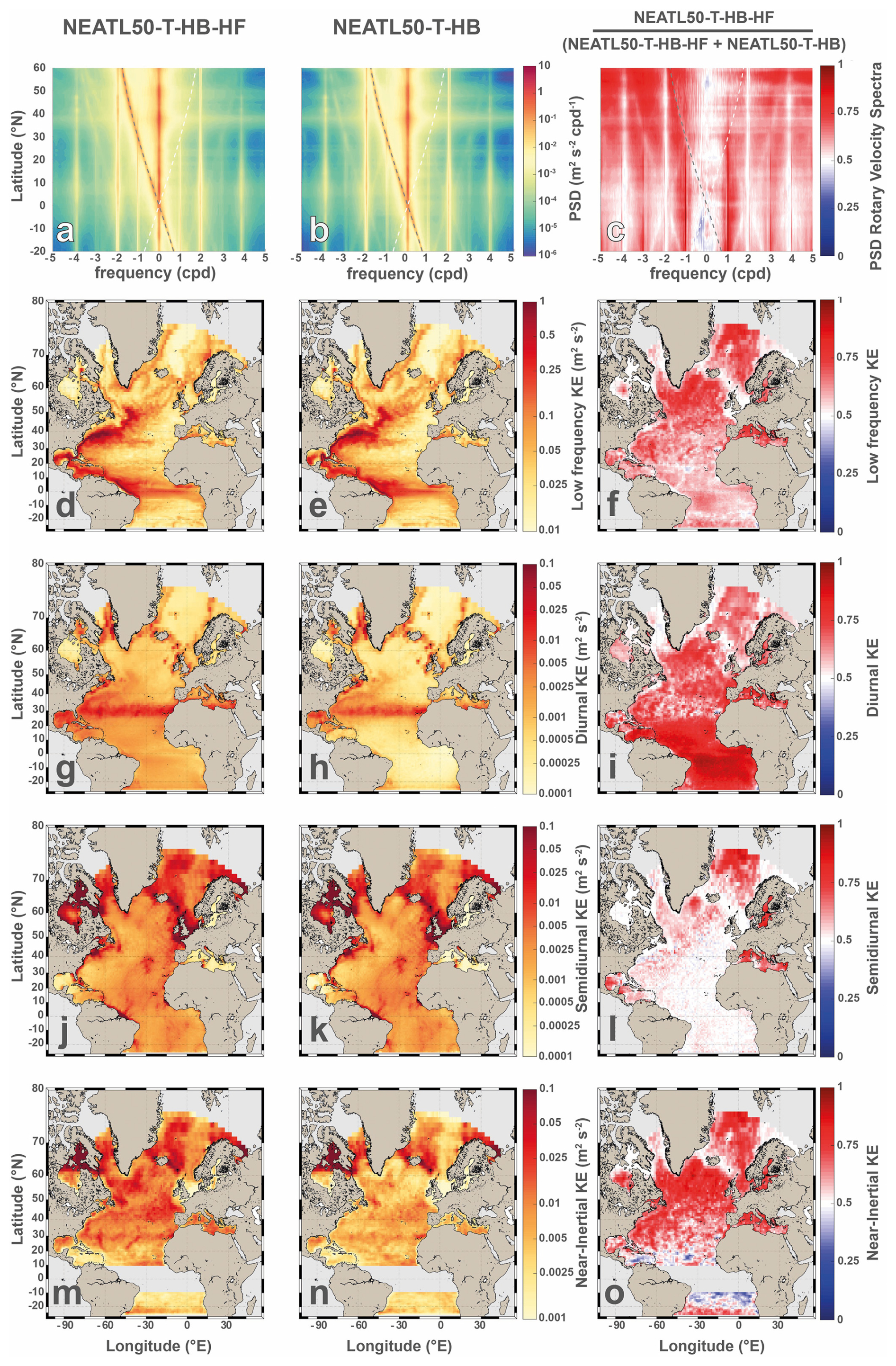
Figure 10 Comparison of NEATL50-T-HB-HF (first column) and NEATL50-T-HB (second column), with a normalized ratio obtained by dividing the first column by the sum of the first and second columns (third column); a ratio of $\mathrm{1}/\mathrm{2}$ indicates equal energies. The first row (a–c) shows the zonally averaged rotary spectra in 1°  latitude bins computed over the offshore domain (waters deeper than 500 m) in the NEATL domain; note the decimal logarithmic color scale for panels (a) and (b). The subsequent rows show maps of surface horizontal kinetic energy (SHKE) components over the NEATL domain: low-frequency ($>-\mathrm{0.5}$ and < 0.5 cpd; second row (d–f)); diurnal (±[0.9, 1.1] cpd; third row (g–i)); semidiurnal (±[1.9, 2.1] cpd; fourth row (j–l)); and near-inertial (±[0.9, 1.1]f cpd restricted poleward of ±5° latitude; fifth row (m–o)). Note the decimal logarithmic color scale for all map panels.

Overall, the increase in wind forcing frequency raises the total SHKE across most of the domain through a gain of high-frequency energy. A strong amplification occurs in the near-inertial band, consistent with the known role of the wind in driving near-inertial motions (Klein et al., 2004; Rimac et al., 2013; Flexas et al., 2019). As noted by several authors (Rimac et al., 2013; Yu et al., 2019; Raja et al., 2022), this near-inertial response is less pronounced in tropical and subtropical regions than at mid-latitudes (Fig. 10o). A more unexpected feature is the strong amplification in the diurnal band almost everywhere and in the semidiurnal band in regions of weak semidiurnal energy such as semi-enclosed basins. This behavior likely reflects the diurnal and semidiurnal cycles of the wind itself (Dai and Deser, 1999; Savazzi et al., 2022; Dai, 2023). In particular, Dai and Deser (1999) estimated globally that the diurnal cycle accounts for 30 %–40 % of the daily wind variance over the ocean, whereas the semidiurnal cycle accounts for only 15 %–25 %. The dominant diurnal share explains why the wind-forced signal covers most of the domain in the diurnal band. The semidiurnal share, by contrast, is small enough that the directly wind-forced response can only emerge clearly where the background astronomical semidiurnal tide is itself weak, which is precisely the case in the semi-enclosed basins where we observe the amplification in the ratio maps. Consistently, no such amplification appears in regions known for resonant astronomical semidiurnal tides, such as the North Sea (e.g., Jänicke et al., 2021), the English Channel and Irish Sea (e.g., Webb, 2013), Hudson Bay (e.g., Cummins et al., 2010), and the Bay of Fundy–Gulf of Maine system (e.g., Garrett, 1972), where the strong astronomical signal is expected to mask the wind-forced response. Note that the diurnal amplification appears weaker near 30° in Fig. 10i.

6 Discussion

The experimental suite analyzed in the previous section allows us to attribute changes in total surface horizontal kinetic energy (SHKE) and its frequency distribution to individual numerical choices (grid and bathymetry resolution, wind and tidal forcing, and wave drag). In this section, we discuss the parameters that most strongly affect the SHKE distribution in each frequency band and, where applicable, how they could be adjusted to reduce the model-drifter gap. Figure 11 synthesizes, for each of the six sensitivity experiments, the relative change in total and per-band SHKE for the offshore (>500 m) and continental-shelf (<500 m) regions. This forms the backbone of the discussion that follows where each of the next paragraphs focuses on one frequency band.

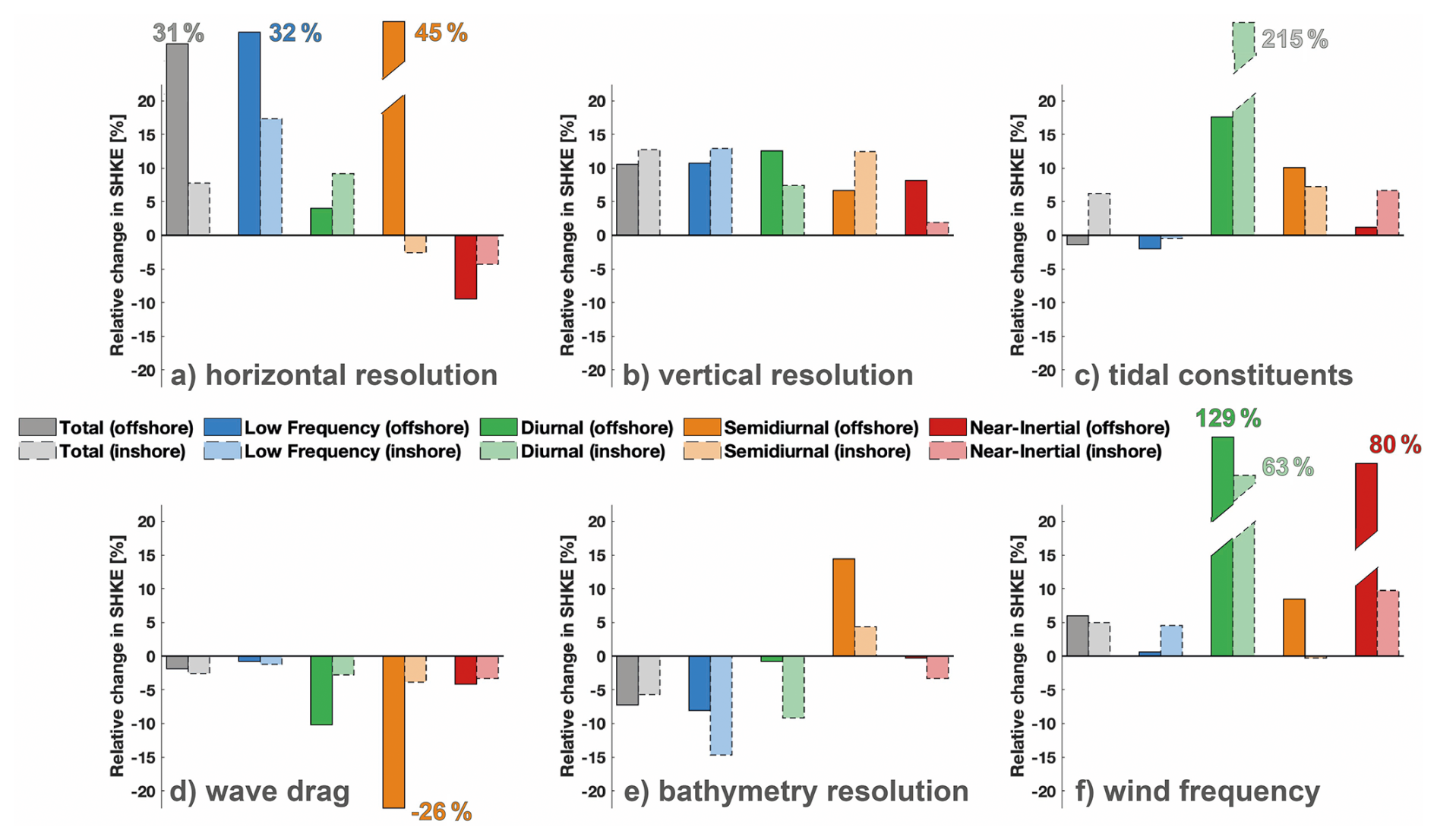
Figure 11 Sensitivity of the domain-averaged surface horizontal kinetic energy (SHKE) to six model configuration choices, separately for the offshore (waters deeper than 500 m; filled bars, solid edges) and continental shelf (waters shallower than 500 m; lighter bars, dashed edges) subdomains of the NEATL region. Each panel shows the relative change in SHKE, $({\mathrm{SHKE}}_{\mathrm{mod}}-{\mathrm{SHKE}}_{\mathrm{ctrl}})/{\mathrm{SHKE}}_{\mathrm{ctrl}}$ (in %), induced by a single parameter modification, decomposed into five components: total SHKE (grey), low-frequency ($>-\mathrm{0.5}$ and < 0.5 cpd, blue), diurnal (±[0.9, 1.1] cpd, green), semidiurnal (±[1.9, 2.1] cpd, orange), and near-inertial (±[0.9, 1.1]f cpd restricted poleward of ±5° latitude, red). The six parameter pairs (control to modified) are: (a) horizontal resolution, NEATL12-T to NEATL50-T; (b) vertical resolution, NEATL12-T to NEATL12-T-HVR; (c) number of tidal constituents, NEATL12-M₂ to NEATL12-T; (d) inclusion of internal wave drag, NEATL50-T to NEATL50-T-WD; (e) bathymetry resolution, NEATL50-T to NEATL50-T-HB; (f) atmospheric forcing temporal frequency, NEATL50-T-HB to NEATL50-T-HB-HF. The vertical axis is clipped at ±20 % for readability; values outside this range are reported numerically above (positive) or below (negative) the corresponding bar.

The total SHKE (grey in Fig. 11) is most sensitive to horizontal resolution in the offshore region, where refining the horizontal grid from $\mathrm{1}/\mathrm{12}$ to $\mathrm{1}/\mathrm{50}\mathit{°}$ increases the offshore SHKE by about one third (+31 %, Fig. 11a). The increase in horizontal resolution is also the parameter that fills the most the high-frequency continuum between the tidal peaks (Garrett and Munk, 1975) by resolving smaller-scale wave modes that feed the continuum through nonlinear wave–wave interactions (Müller et al., 2015). All simulations nevertheless underestimate this continuum relative to drifters, a mismatch that cannot be explained by the Eulerian-Lagrangian distinction and likely reflects both incomplete wave–wave interaction cascades in the models and a contribution of drifter positioning errors to the observed high-frequency variance (Yu et al., 2019). Vertical resolution raises the total SHKE by +10 % offshore and +13 % on the shelf (Fig. 11b), reflecting better-resolved horizontal flows via improved representation of their baroclinic structure (Stewart et al., 2017). This makes vertical resolution the parameter that generate the highest increase on the total shelf SHKE, ahead of horizontal resolution (+8 %, Fig. 11a). Higher-resolution bathymetry is the only parameter that reduces the total SHKE, and it does so on both subdomains (−7 % offshore and −6 % on the shelf, Fig. 11e), because finer bathymetry both enhances lateral and bottom dissipation (Zhai et al., 2010; Ferrari and Wunsch, 2009) and reshapes the large-scale circulation through better-resolved bathymetric gradients (Chassignet and Xu, 2021; Chassignet et al., 2023).

Low frequencies (blue in Fig. 11) dominate the offshore SHKE in both the simulations (83 %–93 %) and the undrogued drifters (64 %–78 %), consistent with large- and mesoscale motions carrying most of the oceanic kinetic energy (Wunsch and Stammer, 1995; Ferrari and Wunsch, 2009; Morrow and Le Traon, 2012). The smaller low-frequency fraction in the drifters reflects the richer high-frequency content of their trajectories, at least partly attributable to measurement artifacts (Elipot et al., 2016; Yu et al., 2019; Arbic et al., 2022) and wind slippage (Niiler and Paduan, 1995; Arbic et al., 2022), rather than a deficit of absolute low-frequency energy. In absolute terms, NEATL50-T-HB-HF concentrates more low-frequency SHKE than the drifters in strong low-frequency motions, while the drifters carry more low-frequency SHKE than the simulations in the weakly energetic basin interiors. We cannot explain these contrasts with our current model set-ups. Three parameters still carry a distinctive signature. Finer horizontal resolution strongly increases the low-frequency SHKE (+32 % offshore and +17 % on the shelf Fig. 11a). Hourly wind forcing drops the offshore low-frequency fraction from 91.4 % to 86.7 %, the only run below 90 %, through the same ratio effect as the drifter comparison, since the higher-frequency wind variability feeds the higher frequency continuum (Flexas et al., 2019) while leaving the absolute offshore low-frequency SHKE nearly unchanged (< 1 %, Fig. 11f). Higher-resolution bathymetry reduces the low-frequency SHKE on both subdomains, more strongly on the shelf, likely reflecting the surface signature of an enhanced transfer of energy toward higher-frequency motions through flow–topography interactions and internal wave generation (e.g., Ferrari and Wunsch, 2009; Nikurashin and Ferrari, 2010; De Marez et al., 2020). Combined with the effect of finer bathymetry reduction of the total SHKE noted above, this suggests that at least part of the low-frequency energy removed from the surface is ultimately dissipated rather than transferred to higher frequencies.

NEATL50-T-HB-HF overestimates the observed drifter diurnal SHKE (green in Fig. 11) equatorward of diurnal critical latitude (i.e., 30° N) and underestimates it poleward. Three parameters dominate this band in Fig. 11. Hourly wind forcing more than doubles the offshore diurnal SHKE (+131 %, Fig. 11f) with a nearly uniform spatial pattern, consistent with the diurnal cycle of the wind (Dai and Deser, 1999; Savazzi et al., 2022; Dai, 2023). Expanding the tidal forcing from M₂ only to the eight largest constituents more than triples the diurnal SHKE on the shelf (+233 %, Fig. 11c), where the barotropic tidal currents are strongest (Pugh and Woodworth, 2014), while leaving the offshore signal poleward of 30° N nearly unchanged. Internal wave drag is absent following Xu et al. (2022), who adopted the Arbic et al. (2010) approach of tuning wave drag to fit observed tides and found that a zero drag scale minimizes the barotropic M₂ RMS error in NEATL tidal configuration. When reintroduced in NEATL50-T-WD, internal wave drag (Jayne and St. Laurent, 2001) acts on the diurnal band only equatorward of the diurnal critical latitude (Fig. 11d), consistent with its selective action on propagating internal tides. The poleward deficit in NEATL50-T-HB-HF diurnal SHKE is non-tidal, and among our tested parameters only increased wind forcing frequency acts on this signal. In contrast, the equatorward excess is of tidal origin, and the inclusion of a weak topographic wave drag as discussed in Xu et al. (2022) stands out as a concrete and testable path to bring the simulated diurnal SHKE closer to the drifter observations equatorward of 30° N.

In the semidiurnal band (orange in Fig. 11), the distortion introduced by the Lagrangian sampling is the largest (Sect. 4) and prevents the use of the drifters as reference. Three parameters dominate this band in Fig. 11. Higher-resolution bathymetry raises the semidiurnal SHKE on both subdomains despite reducing the total SHKE (Fig. 11e), consistent with stronger barotropic-to-baroclinic conversion at a better-resolved shelf-break topography (Niwa and Hibiya, 2011; Buijsman et al., 2020; Xu et al., 2022), particularly clear for the well-known Amazon source of semidiurnal internal tides (Beardsley et al., 1995; Tchilibou et al., 2022). Finer horizontal resolution reduces the shelf semidiurnal fraction by −3 % (Fig. 11a), a change that seems small but is meaningful relative to the +8 % shelf total increase, indicating enhanced shelf-break conversion that feeds internal tides radiating seaward, consistent with the predominantly barotropic nature of the shelf semidiurnal tide and with the dissipation of a large share of the global M₂ energy over continental shelves (Egbert and Ray, 2001). The corresponding +45 % offshore increase is large in relative terms but represents only an absolute shift from 1.9 % to 2.0 % of the total SHKE. Yu et al. (2019) also suggested that insufficient horizontal resolution could enhance the semidiurnal peak by inhibiting scattering into the wave continuum (Müller et al., 2015; Shriver et al., 2012). This mechanism could additionally contribute to the shelf semidiurnal reduction, but raises the question of why a comparable reduction is not apparent in the deep ocean. Internal wave drag cuts the offshore semidiurnal SHKE by about one quarter (−27 %) while barely affecting the total (Fig. 11d), in line with the interpretation of Yu et al. (2019) and Arbic et al. (2022) that the semidiurnal excess in tide-forced models reflects in part the absence of such a drag. This reduction is spatially concentrated away from the Gulf of Mexico-Gulf Stream pathway, suggesting a weaker imprint of wave drag in regions of strong western boundary currents. The excess in semidiurnal SHKE in OP Seed drifters when compared to measurements is predominantly in the deep ocean, exactly where wave drag preferentially acts. As for the diurnal band, adding a weak topographic wave drag may bring the simulated semidiurnal SHKE closer to the drifter observations, damping the model excess in the deep ocean without altering the western boundary current signal.

Finally, in the near-inertial band (red in Fig. 11) , the drifters carry more SHKE than NEATL50-T-HB-HF over the same regions of strong low-frequency motions as in the semidiurnal band as well as near the low-latitude equatorial edge of the band. Two parameters dominate this band in Fig. 11. Hourly wind forcing nearly doubles the offshore near-inertial fraction (from 4.5 % to 7.6 %, corresponding to a +80 % absolute increase, Fig. 11f), and produces a more modest rise on the shelf, consistent with winds being a major source of near-inertial motions (Klein et al., 2004; Rimac et al., 2013). As noted by Rimac et al. (2013) and Yu et al. (2019), this increase is less pronounced in tropical and subtropical regions than at mid-latitudes. Finer horizontal resolution acts in the opposite direction. Although the absolute near-inertial SHKE rises along with the overall SHKE increase, the fraction of total SHKE stored in this band drops (Fig. 11a) both offshore (from 6.1 % of total SHKE to 4.2 %) and on the shelf (from 20.3 % of total SHKE to 18 %). A natural interpretation would invoke a more efficient vertical transport of near-inertial kinetic energy into the ocean interior through the better-resolved mesoscale and submesoscale fields (e.g., Kunze, 1985; Thomas et al., 2020; Lu et al., 2023). However, the spatial pattern does not straightforwardly support this view, since the reduction is not systematically concentrated in the most energetic regions of the domain but rather appears in the basin interior, leaving the origin of this near-inertial deficit at higher resolution as an open question.

7 Conclusions

In conclusion, this study used six pairwise twin experiments, each isolating a single numerical choice, to quantify how individual model parameters shape the surface horizontal kinetic energy (SHKE) distribution in the North and Equatorial Atlantic. Earlier comparisons of SHKE in tide-resolving models to drifter observations (Yu et al., 2019; Arbic et al., 2022) have raised a number of hypotheses on the role of individual parameters in shaping the SHKE distribution, but these hypotheses could not be directly tested because the model pairs they compared differed in several parameters simultaneously. Our twin-experiment design addresses this limitation by changing only one parameter at a time across a dedicated suite of tide-resolving, eddy-resolving to submesoscale-permitting simulations. Although several questions remain open, the design has made it possible to carry out a parameter-by-parameter assessment of the SHKE distribution within a unified diagnostic framework and frequency decomposition, providing a by-band, by-subdomain view of the individual effects of each parameter on the SHKE. This sensitivity picture should be of practical use to anyone designing a future tide-resolving numerical simulation. For the HYCOM NEATL configuration, the natural next step would be to test the inclusion of a topographic internal wave drag in NEATL50-T-HB-HF, which should reduce the tidal-band SHKE excess relative to the drifters equatorward of the respective critical latitudes. The twin-experiment framework could also be extended toward parameters still left untested here, with a particular focus on the mechanisms able to amplify the non-tidal variability away from the low-frequency motions. Two natural candidates are the lateral viscosity and the wind stress formulation, both recently shown to substantially modulate the Gulf Stream pathway and variability in a non-tidal NEATL50 simulation by Chassignet and Xu (2025).