A novel ALE scheme with the internal boundary for true free surface simulation in geodynamic models

The accurate simulation of Earth's surface is essential for understanding lithospheric and mantle dynamics, especially in processes such as subduction and surface deformation. Traditional top boundary conditions, such as free-slip or no-slip, do not fully capture the complex interactions occurring at the surface. The commonly used “Sticky Air” method, while practical, suffers from several limitations, including increased computational cost and marker fluctuation issues. Additionally, free surface numerical fluctuations, known as the “drunken sailor instability”, are characteristic of all free surface simulations, including true Lagrangian free surface treatments and Arbitrary Lagrangian–Eulerian (ALE) methods. In this study, we propose a novel scheme within the finite element framework that integrates the “Sticky Air” concept into an ALE formulation by employing an internal boundary to simulate a true free surface, referred to as the ALE-IB. This approach effectively addresses the limitations of existing methods, notably by reducing marker fluctuation issues and enhancing numerical stability. Moreover, it maintains a true surface in the computational domain that can be further reshaped by surface processes such as erosion and deposition, and provides a foundational scheme for further coupling framework of tectonic modelling and landscape evolution modelling. We detail the theoretical formulation, implementation strategies, and validation through a series of numerical experiments. The results demonstrate that our method achieves higher accuracy and broader applicability compared to conventional techniques. Ultimately, this framework provides a more realistic and robust tool for geodynamic modelling of the Earth's free surface.

1 Introduction

The Earth's surface serves as the interface beneath the atmosphere where normal and shear stresses are negligible. It deforms freely in response to a combination of various processes, including surface processes, tectonic activity, mantle convection, and their interactions (Willett, 1999; Braun, 2010). Historically, most geodynamic simulations, particularly those focusing on mantle convection, have utilized either free-slip or no-slip boundary conditions at the surface. However, further studies have highlighted the significance of treating the Earth's surface as a free surface in the context of lithospheric and mantle dynamics (Zhong et al., 1996; Kaus et al., 2010). For instance, in the case of free subduction, the free surface plays a crucial role in influencing the dynamics, including the morphology and timing of slab descent (Schmeling et al., 2008; Crameri and Tackley, 2016). Currently, there is a growing reliance on numerical models that incorporate a true free surface in related studies (Rose et al., 2017).

Several approaches have been developed to simulate the free surfaces in geodynamic models:

1. True Free Surface via Conforming Mesh Methods: This approach allows the mesh to adapt to the topography, enabling the application of a zero normal stress condition at the surface. This configuration can employ either a deforming Lagrangian grid (Poliakov and Podladchikov, 1992) or an Arbitrary Lagrangian–Eulerian (ALE) framework (Fullsack, 1995; Kaus et al., 2008; Beaumont et al., 1994; Pysklywec et al., 2000) (Fig. 1a). A notable limitation of Lagrangian algorithms is their requirement for frequent remeshing to accommodate significant distortions. By integrating Lagrangian and Eulerian methodologies, the ALE framework can enhance computational efficiency for specific problems (Donea et al., 2004).

2. Pseudo-Free Surface via Non-Conforming Methods with Eulerian Mesh: This approach involves discretizing or tracing the surface independently through various techniques. In Zhong et al. (1996), the surface coordinates are updated as additional variables based on vertical velocity, subsequently applying the resulting topography as a normal stress boundary condition at the top of the Eulerian grid. However, this method is inadequate for scenarios such as folding or subduction, where vertical deformation is non-uniform and horizontal components are important. Alternative methods, such as the Marker-in-Cell method (Harlow and Welch, 1965) and level-set functions (Braun et al., 2008; Hillebrand et al., 2014), are commonly employed. These free-surface tracking methods facilitate the identification of cells within the flow grid that contain the interface, enabling the direct application of free-surface boundary conditions to these interface cells.

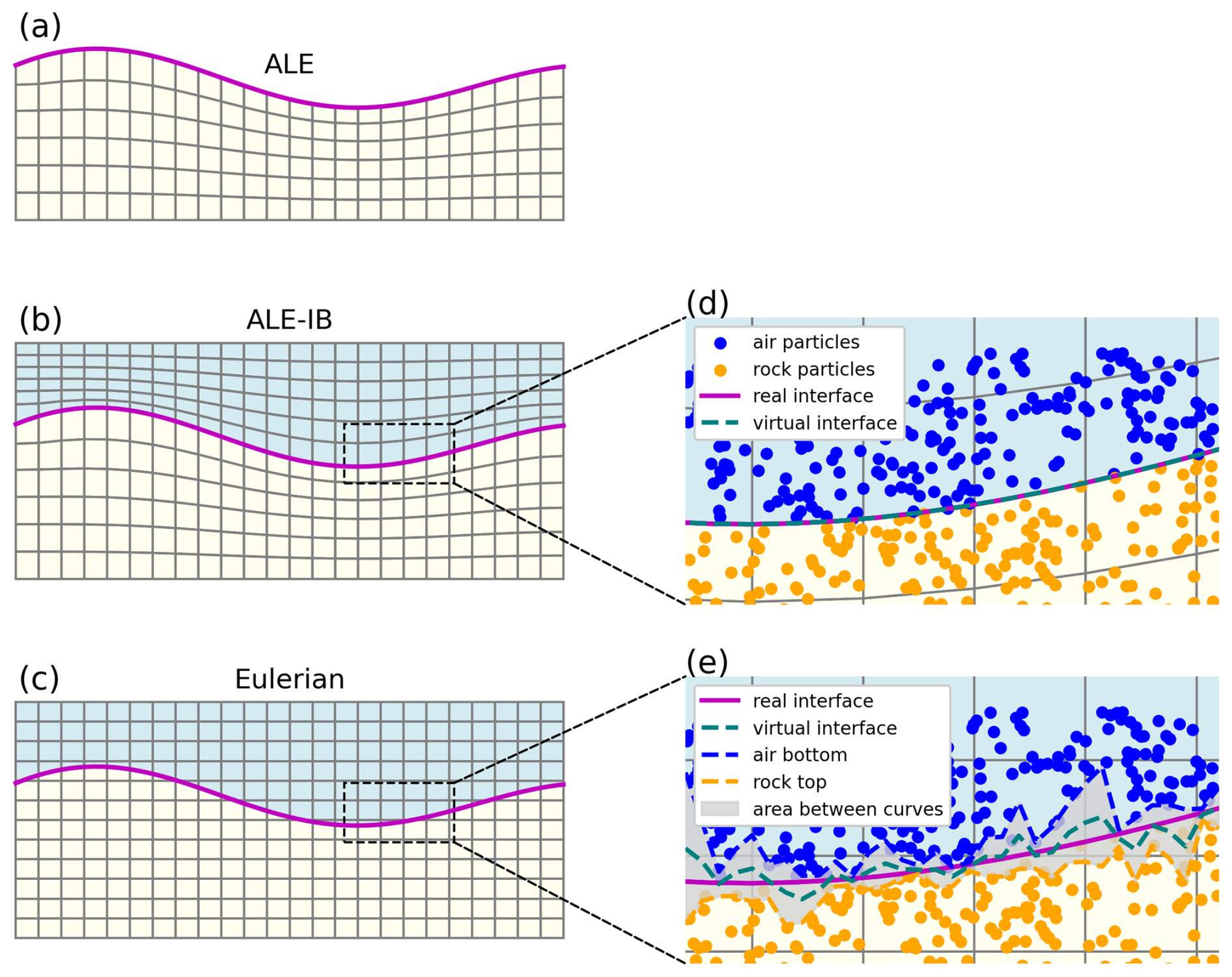
Figure 1 Classification of methods used for simulating a free surface (indicated by the magenta line). Colored points represent markers for different materials. Methods include: (a) ALE scheme, (b) ALE scheme with the internal boundary (ALE-IB) and the “sticky air” method, and (c) Eulerian scheme with the “sticky air” method. The real interface refers to the actual free surface, while the virtual interface represents the surface obtained from numerical modelling.

Within the Pseudo-Free Surface framework, a widely-used approach is the “Sticky Air” method (Matsumoto and Tomoda, 1983; Zaleski and Julien, 1992; Gerya and Yuen, 2003; Quinquis et al., 2011; Schmeling et al., 2008; Crameri et al., 2012) (Fig. 1c), combining the use of Lagrangian advecting points (markers, tracers or particles) with an Eulerian grid, which has gained popularity in recent studies (Hillebrand et al., 2014; Crameri and Tackley, 2016; Deng et al., 2024). In this approximation, a low-viscosity, low-density fluid layer (referred to as “air” or “water”) is situated above the free surface. Typically, either a free-slip boundary condition or an open boundary condition is implemented above this fluid layer. Importantly, the “sticky air” layer is not intended to represent a physical reality. It has a density similar to air but a viscosity that is on the order of 10²²–10²⁴ times greater. Instead, it serves as a conceptual construct for free surface simulation within the computational model (Babel and Vinck, 2022). The evaluation of the “sticky air” technique, along with its applicable conditions and limitations, is thoroughly discussed in Crameri et al. (2012).

While the Sticky Air method offers simplicity in implementation, it also presents several limitations (Duretz et al., 2016). Notably, it increases computational costs due to the necessity of extending the model domain to accommodate the low-viscosity air layer. The accuracy of the free surface approximation heavily depends on the viscosity and thickness of this layer (Crameri et al., 2012). When combined with markers, issues such as “marker fluctuation” (Fig. 1e) can arise, particularly when extracting the free surface from regions between air and lithosphere material points. In such cases, air markers may be subducted along with the lithosphere (Schmeling et al., 2008; Hillebrand et al., 2014). To overcome these limitations, Duretz et al. (2016) proposed an interface capturing technique; however, this approach was developed within the context of a staggered grid finite difference scheme, which limits its direct applicability within finite element frameworks.

We propose a novel scheme for modelling the true free surface within finite element method (FEM), which integrates the “sticky air” approach into the ALE scheme. This method employs an internal boundary to accurately represent the free surface, referred to as ALE-IB (Fig. 1b). We implement this scheme for free surface simulations in the geodynamic codes Underworld 2 (Moresi et al., 2007; Mansour et al., 2020) and Underworld 3 (Moresi et al., 2025a). Our approach includes a detailed explanation of the theoretical foundations and implementation steps, showcasing how the ALE-IB scheme enhances accuracy and stability. We conduct numerical experiments to validate our method, comparing results with analytical solutions and other free surface modeling techniques. These comparisons highlight the advantages of our scheme in terms of precision and computational efficiency, making it a valuable tool for complex geodynamic simulations.

2 Method

2.1 Governing Equations

For the tectonic modelling, we assume that the Earth's lithosphere and mantle deform like the incompressible viscous fluid on geological time scales. The behaviour of the fluid follows a set of equations covering momentum, mass (Moresi et al., 2007):

$$\begin{array}{}\text{(1a)}& {\displaystyle }& {\displaystyle }\mathrm{\nabla }\cdot \mathit{\sigma }-\mathrm{\nabla }p=\mathit{f},\text{(1b)}& {\displaystyle }& {\displaystyle }\mathrm{\nabla }\cdot \mathit{u}=\mathrm{0},\text{(1c)}& {\displaystyle }& {\displaystyle }\mathit{\rho }{C}_p\left({\displaystyle \frac{\partial T}{\partial t}}+\mathit{u}\cdot \mathrm{\nabla }T\right)=\mathrm{\nabla }\cdot \left(k\mathrm{\nabla }T\right)+\mathit{\rho }H,\end{array}$$

where σ is the deviatoric stress tensor, p is the pressure, f=ρg is the force term, ρ is the density and g is the gravity acceleration, u is the velocity, C_p is the heat capacity at constant pressure, T is the absolute temperature, k is thermal conductivity, and H is the (radiogenic) heat production per unit mass.

The following boundary conditions are considered here:

$$\begin{array}{}\text{(2)}& {\displaystyle }& {\displaystyle }\text{No slip: }\mathit{u}=\mathrm{0},\text{(3)}& {\displaystyle }& {\displaystyle }\text{Free slip: }\mathit{u}\cdot \mathit{n}=\mathrm{0},\text{(4)}& {\displaystyle }& {\displaystyle }\text{Free surface: }\mathit{\sigma }\cdot \mathit{n}=\mathrm{0}.\end{array}$$

2.2 Numerical Implementation

2.2.1 Underworld 2

These Eq. (1) are solved numerically by using the particle-in-cell and finite element method (PIC-FEM) code Underworld 2 (Moresi et al., 2007; Mansour et al., 2020). Underworld 2 is a Python-friendly version of the Underworld code (Moresi et al., 2002, 2003), offering a programmable and flexible interface to its comprehensive functionality, designed to run efficiently in a parallel HPC environment. In Underworld 2, the hybrid particle/mesh algorithms enable the tracking of historical information via Lagrangian integration points, while the structured computational mesh provides an efficient solution to the Stokes equation using multigrid.

2.2.2 Underworld 3

Underworld 3 is a geophysical fluid dynamics modelling framework built on the PIC-FEM methodology (Moresi et al., 2025a). It evolves from earlier versions of Underworld and incorporates several key design features: (1) a symbolic interface and symbolic forms for constructing finite element representations using SymPy (Meurer et al., 2017) and Cython (Behnel et al., 2010), (2) fast, robust, and parallel numerical solvers powered by PETSc (Balay et al., 2024) and petsc4py (Dalcin et al., 2011), (3) Lagrangian particles for effectively managing transport-dominated variables, and (4) support for using unstructured and adaptive meshing.

3 Numerical implementation of free surface simulations

3.1 Sticky air method in Eulerian scheme

Several of our experiments employ an approximation of Earth's surface using the “sticky air” method in the Eulerian scheme (Schmeling et al., 2008; Crameri et al., 2012) for comparative analysis. This approach allows the modelling of topographic variations within a purely Eulerian framework by introducing an upper layer of sticky air. The density of this layer is set close to zero for ensuring it exerts no pressure on the actual free surface (the interface between the air and rock), or it is set to 1000 kg m⁻³ to approximate a water-loaded free surface (Gerya and Yuen, 2003). Crameri et al. (2012) investigated the influence of the viscosity contrast and the thickness of the sticky air layer and concluded that, for this method to produce reliable results, certain conditions must be satisfied. One such condition is that the isostatic compensation factor (Crameri et al., 2012) must be considered:

$$\begin{array}{}\text{(5)}& {\displaystyle }{\displaystyle }{C}_{\text{isost}}={\displaystyle \frac{\mathrm{3}}{\mathrm{16}{\mathit{\pi }}^{\mathrm{3}}}}{\left({\displaystyle \frac{L}{h_{\text{st}}}}\right)}^{\mathrm{3}}{\displaystyle \frac{{\mathit{\eta }}_{\text{st}}}{{\mathit{\eta }}_{\text{ch}}}},\end{array}$$

where L is the box width, h_st and η_st denote the thickness and viscosity of the sticky air layer, respectively, and η_ch represents the characteristic viscosity controlling relaxation, typically approximated by the mantle viscosity. C_isost is a nondimensional combination of geometric and material parameters that quantifies the ratio of dynamic stresses to the static pressure scale set by the system. When C_isost≪1, the surface exhibits near-isostatic behavior over the relevant timescale. This means the pressure field can adjust effectively to balance loads, resulting in minimal residual traction on the surface. Consequently, the error introduced by the “sticky air” method is small.

The upper boundary condition over the air layer can be modeled as either free-slip or open (zero stress). As discussed in Hillebrand et al. (2014) and Deng et al. (2024), an open boundary condition can suppress the return flow of sticky air, which is usually generated under a free-slip boundary condition, thereby reducing the velocity of the air layer. For an open top boundary, the thickness of the sticky air layer does not need to be sufficiently large as indicated by Eq. (5). However, for the purpose of consistent comparison with previous studies (Kaus et al., 2010; Rose et al., 2017), all our experiments employ a free-slip boundary condition at the top of the air layer and utilize a relatively thick air layer.

3.2 True free surface in ALE with the internal boundary scheme

We implement the true free surface simulation in ALE-IB scheme. Generally, the mesh undergoes regridding to align with the free surface through the following steps, similar to ALE scheme (Thieulot, 2011; Rose et al., 2017) (See Fig. 3):

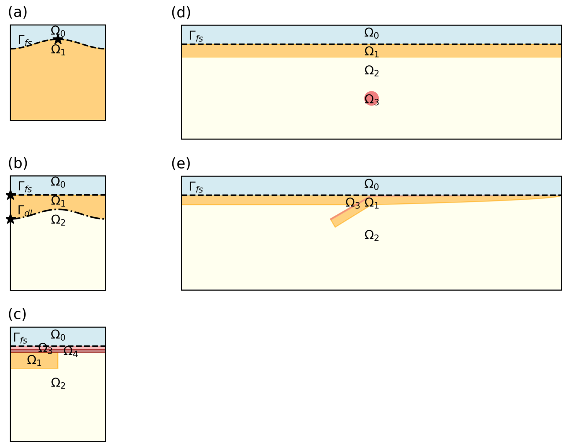
Figure 2 Model setup for (a) viscous relaxation of sinusoidal topography, (b) Rayleigh–Taylor instability, (c) delamination, (d) rising sphere, and (e) subduction. Ω indicates different material domains, with Ω₀ specifically representing the air domain – used only in Eulerian and ALE-IB schemes. The dashed line marks the free surface Γ_fs, and the stars denote tracer locations used in some experiments.

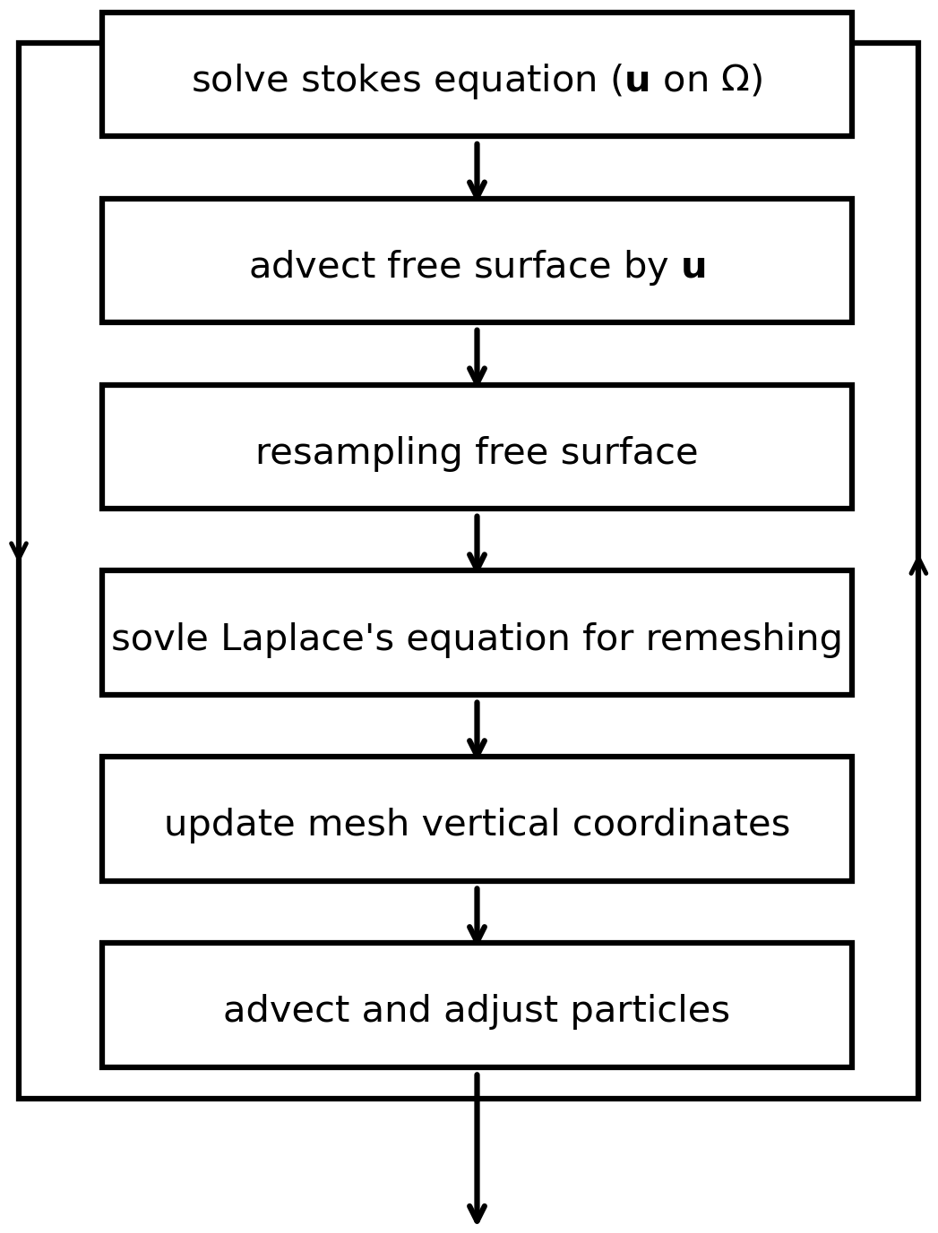
Figure 3 Flowchart presenting the free surface simulation within the ALE framework with internal boundary.

1. Free Surface Advection

   The mesh nodes along the internal boundary represent the discrete free surface of the domain. Their location coordinates, denoted as X, is advected forward in time using displacements determined by the forward Euler scheme:

   $$\begin{array}{}\text{(6)}& {\displaystyle }{\displaystyle }{X}^{n+\mathrm{1}}=X^n+\mathrm{\Delta }t{\mathit{u}}^n\text{ on }{\mathrm{\Gamma }}_{\text{fs}},\end{array}$$

   where Γ_fs indicates the location of the time-dependent free surface. When coupled with surface processes, X will also be influenced by these processes.

2. Free Surface Resampling

   In accordance with the ALE scheme, the x coordinates X_x in 2D or the x, y coordinates X_x,y in 3D of the mesh nodes remain constant. Consequently, we need to resample the vertical coordinates X_z at these specified locations.

3. Mesh Regridding

   To achieve a uniform distribution of displacements D_z in the vertical mesh coordinates, we solve Laplace's equation:

   $$\begin{array}{}\text{(7)}& {\displaystyle }{\displaystyle }{\mathrm{\nabla }}^{\mathrm{2}}{D}_z=\mathrm{0}\end{array}$$

   The boundary conditions applied here are Dirichlet constraints, which define the top and bottom boundaries as zero and the internal boundary as new displacement ($D_z=X_z^{n+\mathrm{1}}-X_z^n\text{ on }{\mathrm{\Gamma }}_{\text{fs}}$).

Next, we update the vertical mesh coordinates forward in time using displacements determined by the forward Euler scheme:

$$\begin{array}{}\text{(8)}& {\displaystyle }{\displaystyle }{X}_z^{n+\mathrm{1}}=X_z^n+D_z.\end{array}$$

Stabilisation method

Most approaches to free surface simulations have faced instability, often referred to as “sloshing instability” or the “drunken sailor effect” (Kaus et al., 2010). This instability arises from the significant density contrast typically encountered at a free surface (e.g. the rock-air interface in the “sticky air” method), which severely restricts the maximum stable timestep for computations. In many cases, the maximum stable timestep is considerably smaller than the viscous relaxation time (Andrés-Martínez et al., 2015), often several orders of magnitude less than that of an equivalent model with free-slip boundary conditions.

To address this timestep limitation, stabilization methods such as the Free Surface Stabilization Algorithm (FSSA) proposed by Kaus et al. (2010) are necessary. This approach enhances the standard element stiffness matrix by incorporating a surface traction term. Andrés-Martínez et al. (2015) introduces a further version of FSSA, which differs from the original by applying the stabilization only at the free surface, rather than at every element boundary. Additionally, Kramer et al. (2012) utilizes implicit time integration to simulate the free surface effectively. The applications of FSSA are tested in the Rayleigh–Taylor model (Rose et al., 2017) and in ice-sheet models (Löfgren et al., 2022).

An advantage of the ALE-IB scheme is its flexibility in directly applying boundary conditions to the free surface, similar to the ALE method. In this study, we employ a simpler FSSA method akin to the one from Andrés-Martínez et al. (2015) by incorporating the traction term F_fs into the Neumann boundary condition at the free surface:

$$\begin{array}{}\text{(9)}& {\displaystyle }{\displaystyle }{F}_{\text{fs}}=\mathrm{\Theta }\mathrm{\Delta }t\underset{\mathrm{\Gamma }}{\int }\left(\mathrm{\Delta }\mathit{\rho }\mathit{g}\right)(\mathit{n}\cdot \mathit{u}\cdot \mathit{n})\mathrm{d}\mathrm{\Gamma },\end{array}$$

where Δt is the set time step, Δρ is the density contrast across the free surface, Γ denotes the boundary surface. Θ is the controlling factor, with the optimal value being 0.5, as noted in Kaus et al. (2010).

4 Numerical experiments

We consider five numerical experiments to evaluate and compare the accuracy and stability of three free surface simulation algorithms: (1) the true free surface implemented within an ALE scheme, (2) the sticky air method within an Eulerian scheme, and (3) the true free surface within an ALE scheme combined with the sticky air method and internal boundary (ALE-IB). The experiments include (panel a) viscous relaxation of sinusoidal topography, (panel b) Rayleigh–Taylor instability, (panel c) delamination, (panel d) rising sphere, and (panel e) subduction (Fig. 2). In all cases, the surface boundary condition in the ALE scheme is zero normal stress. For the ALE-IB and Eulerian schemes, a sticky air layer Ω₀ with zero density and low viscosity is placed atop the domain. The first experiment is conducted in Underworld 2 and Underworld 3, while the other experiments are conducted in Underworld 2.

4.1 Topography relaxation

The loading of the Earth's surface can be described as the initial periodic surface displacement of an isoviscous fluid within the infinite half-space (Turcotte and Schubert, 2002). The setup is shown in Fig. 2a. The initial free surface displacement is given by:

$$\begin{array}{}\text{(10)}& {\displaystyle }{\displaystyle }w(x,\mathrm{0})=w_{\mathrm{0}}\cos \left(kx\right),\end{array}$$

where w₀=10 km is the initial load amplitude, $k=\mathrm{2}\mathit{\pi }/\mathit{\lambda }$ is the wave number, with λ=D (the wavelength). D=500 km is the depth of the model domain.

The analytical solution for the decay of topography is characterized by the relaxation time t^* (Zhong et al., 1996; Kramer et al., 2012):

$$\begin{array}{}\text{(11)}& {\displaystyle }{\displaystyle }w(x,t)=w(x,\mathrm{0}){\mathrm{e}}^{-t/t^{*}},\end{array}$$

with the relaxation time t^*:

$$\begin{array}{}\text{(12)}& {\displaystyle }{\displaystyle }{t}^{*}={\displaystyle \frac{Dk+\sinh \left(Dk\right)\cosh \left(Dk\right)}{{\sinh }^{\mathrm{2}}\left(Dk\right)}}{t}_{\mathrm{0}}^{*},t_{\mathrm{0}}^{*}={\displaystyle \frac{\mathrm{2}k\mathit{\eta }}{\mathit{\rho }g}},\end{array}$$

where η is the viscosity, ρ is the density. When λ≪D, $t^{*}\approx t_{\mathrm{0}}^{*}$.

The computational domain is 500 km×500 km for the ALE scheme, and 500 km×600 km for ALE-IB and Eulerian schemes. A constant time step of ${\mathrm{10}}^{-\mathrm{2}}{t}^{*}$ here was employed, with Q₁dQ₀ finite elements and with a mesh of 51×51 nodes (or 51×61 nodes for the larger domain with the air layer). Material properties are: ρ=3300 kg m⁻³ and η=10²¹ Pa s for the lithosphere layer, ρ=0 kg m⁻³ and η=10¹⁸ Pa s for the air layer. Gravitational acceleration is g = 9.81 m s⁻². The side boundaries are free-slip, the bottom is no-slip, and the top boundary is either a free surface or free-slip (over sticky air).

4.2 Rayleigh–Taylor instability

The Rayleigh–Taylor instability model is adapted from Kaus et al. (2010) and Duretz et al. (2011) (See Fig. 2b). A dense and more viscous layer (ρ=3300 kg m⁻³, η=10²¹ Pa s) is sinking through a less dense fluid (ρ=3200 kg m⁻³, η=10²⁰ Pa s). Side boundaries are free slip, the bottom boundary is no-slip and the top boundary is a free surface or free-slip (sticky air). The domain size is 500 km×500 km for ALE scheme and 500 km×600 km for ALE-IB and Eulerian scheme, with Q₁dQ₀ elements and 51×51 nodes (or 51×61 nodes). The initial perturbation has an amplitude of 5 km. A constant time step of 2500 years was employed in the simulations.

4.3 Delamination

This experiment builds upon the models developed in Beall et al. (2017) to examine conditions leading to triggered dripping and lithospheric delamination (See Fig. 2c). The model domain includes a layered crust and mantle with the following parameters: upper crust (20 km thick, ρ=2800 kg m⁻³, η=10²³ Pa s), lower crust (20 km thick, ρ=3300 kg m⁻³, η=10¹⁹ Pa s), lithosphere (100 km thick, ρ=3300 kg m⁻³, η=10²¹ Pa s), and mantle (ρ=3250 kg m⁻³, η=10¹⁸ Pa s). Side boundaries are free slip, the bottom boundary is no-slip and the top boundary is a free surface or free-slip, depending on the simulation scheme. For free surface simulations in ALE-IB and Eulerian scheme, there is a sticky air layer with ρ=0 kg m⁻³, and viscosity of η=10¹⁹ Pa s, 150 km thickness, bordered with free-slip top boundary condition. The computational domain is 900 km×600 km in size for the Eulerian scheme with free-slip top boundary and free surface within ALE scheme, 900 km×750 km in size for free surface in ALE-IB and Eulerian schemes). The mesh employs Q₁dQ₀ elements and 193×129 nodes (or 193×161 nodes).

4.4 Rising Sphere

The rising sphere model is adapted from Case 2 in Crameri et al. (2012) for validating the sticky air approach (See Fig. 2d). A plume with a radius of r_p = 50 km, a density of ρ_p=3200 kg m⁻³, and viscosity of η_p=10²⁰ Pa s, is initially centred at (0, −400 km) of the mantle with ρ_m=3300 kg m⁻³, and viscosity of η_m=10²¹ Pa s. The lithosphere, with ρ_l=3300 kg m⁻³ and viscosity of η_l=10²³ Pa s, has a thickness of 100 km. For simulations in ALE-IB and Eulerian schemes, there is a sticky air layer with ρ=0 kg m⁻³, and viscosity of η=10¹⁹ Pa s, bordered with free-slip top boundary condition. Side boundaries are free slip, the bottom boundary is no-slip. The model domain is 2800 km×700 km in size for ALE scheme (2800 km×850 km in size for ALE-IB and Eulerian schemes), discretized with Q₁dQ₀ elements and 561×281 nodes (or 561×341 nodes).

4.5 Subduction

Models with a free surface boundary condition produce more realistic slab bending, dip angles, and stress states compared to free-slip models, as shown in Kaus et al. (2010). The free surface approach more accurately captures topographic features, whereas free-slip models tend to exhibit more short- and intermediate-wavelength components in the simulated topography (Zhong et al., 1996; Quinquis et al., 2011; Crameri et al., 2017).

The subduction model is modified from Crameri et al. (2017) (See Fig. 2e). It is a thermo-mechanical model designed to simulate the subduction of a visco-plastic slab into the mantle and generate realistic topography signals. The simulation here is run over a short duration with side boundaries are free slip. In contrast to Crameri et al. (2017), where the driving force is based on the temperature-dependent Rayleigh number, here the body force is driven by the same density contrast used in the previous experiments. The materials are assigned a temperature-dependent density, expressed as:

$$\begin{array}{}\text{(13)}& {\displaystyle }{\displaystyle }\mathit{\rho }={\mathit{\rho }}_{\mathrm{0}}(\mathrm{1}-\mathit{\alpha }\mathrm{\Delta }T),\end{array}$$

where α is the thermal expansion coefficient, $\mathrm{\Delta }T=T-T_{\mathrm{0}}$ with T being the temperature, and ρ₀ is the reference density at the reference temperature T₀=300 K.

To simulate the deformation of the subducted lithosphere and surrounding mantle, a visco-plastic rheology is employed. The model uses the Drucker–Prager yield criterion with a pressure-dependent yield stress based on Byerlee's law, which approximates brittle behavior. Frictional-plastic deformation occurs when the stress exceeds the frictional-yield stress σ_y:

$$\begin{array}{}\text{(14)}& {\displaystyle }{\displaystyle }{\mathit{\sigma }}_y=C+P\mathit{\mu },\end{array}$$

where P, C, and μ are the pressure, cohesion and friction coefficient respectively.

The effective plastic viscosity is given by:

$$\begin{array}{}\text{(15)}& {\displaystyle }{\displaystyle }{\mathit{\eta }}_{\text{eff}}^{\text{pl}}={\displaystyle \frac{{\mathit{\sigma }}_y}{\mathrm{2}\dot{\mathit{ϵ}}}},\end{array}$$

Where $\dot{\mathit{ϵ}}$ is the strain rate.

Table 1 Model parameters applied in subduction experiment

Viscous deformation is modeled with a thermally activated power-law rheology, expressed by:

$$\begin{array}{}\text{(16)}& {\displaystyle }{\displaystyle }{\mathit{\eta }}_{\text{eff}}^{\text{vcreep}}={\displaystyle \frac{\mathrm{1}}{\mathrm{2}}}{A}^{\frac{-\mathrm{1}}{n}}\exp \left({\displaystyle \frac{E}{nRT}}\right),\end{array}$$

where A is the pre-factor set as the effective viscosity giving the reference viscosity at T = 1600 K, E is the activation energy, n is the stress exponent, R is the gas constant and T is the temperature.

The effective viscosity combines brittle and ductile rheologies as:

$$\begin{array}{}\text{(17)}& {\displaystyle }{\displaystyle }{\mathit{\eta }}_{\text{eff}}=min({\mathit{\eta }}_{\text{eff}}^{\text{vcreep}},{\mathit{\eta }}_{\text{eff}}^{\text{pl}}),\end{array}$$

and is limited within nine orders of magnitude by applying upper and lower bounds: η_max=10⁵η₀ and ${\mathit{\eta }}_{\text{min}}={\mathrm{10}}^{-\mathrm{4}}{\mathit{\eta }}_{\mathrm{0}}$. where η₀ is a reference viscosity.

An initial weak hydrated crustal layer of 7.5 km thickness is included on top of the subducting plate. Additionally, a sticky air layer with ρ=0 kg m⁻³, and viscosity of η=10¹⁹ Pa s, is implemented, bordered by a free-slip top boundary in the Eulerian and ALE-IB schemes. The model assumes ongoing subduction, represented by a finite-length initial slab. An initial divergent plate boundary is specified at the tail of the subducting plate, with the boundary layer thickness W_BL increasing away from this spreading centre toward the subduction zone according to the $\sqrt{\text{age}}$-law (Crameri et al., 2017):

$$\begin{array}{}\text{(18)}& {\displaystyle }{\displaystyle }{W}_{\text{BL}}\left(x\right)=W_{\text{BL},\mathrm{0}}\left(x\right)\cdot \sqrt{\mathrm{\Delta }{X}_{\text{sc}}},\end{array}$$

where W_BL,0(x) controls the maximum boundary layer thickness, here set as 100 km, x is the horizontal coordinate, and ΔX_sc is the distance from the spreading centre at any given position x. The radial component of the initial temperature is related to plate thickness as $T_z\left(x\right)=T_{\mathrm{0}}+(T_{\mathrm{1}}-T_{\mathrm{0}})\left(\text{erf}\right(d/\mathrm{2}\sqrt{W_{\text{BL}}\left(x\right)}\left)\right)$, where T₀=300 K is the temperature at the surface (and the top of the model domain), T₁=1600 K is the temperature at the model base, d is depth below the surface.

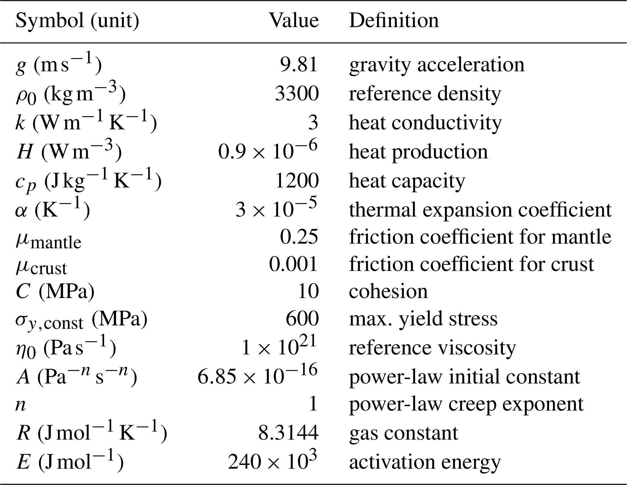
The initial slab is approximately 500 km long, straight from trench to tip, inclined at θ=30° via an abrupt kink, which relaxes during the evolution. All materials share the same heat production rate. The top boundary (and the air layer, if present) is maintained at 300 K, while the bottom boundary is insulated with a zero heat-flux boundary condition. The domain size is 3000 km×800 km for ALE scheme (3000 km×1000 km in size for ALE-IB and Eulerian schemes). It employs Q₁dQ₀ elements and 601×161 nodes (or 201 nodes). Physical and numerical parameter details are given in Table 1.

5 Results and Discussion

5.1 Topography relaxation

In Experiment 1, the initial topography relaxes toward equilibrium over approximately 100 ka. Figure 4 compares the topography obtained from free-surface simulations across three different numerical schemes with the analytical solution Eq. (11). Discrepancies among the schemes are illustrated in Fig. 4a, which shows the temporal evolution of the topography. Figure 4c presents the topography at $\text{Time}=\mathrm{2}{t}^{*}$, approximately equal to 49.21 ka. Both the ALE and ALE-IB schemes demonstrate good agreement with the analytical solution, whereas the Eulerian scheme exhibits fluctuations that reduce accuracy.

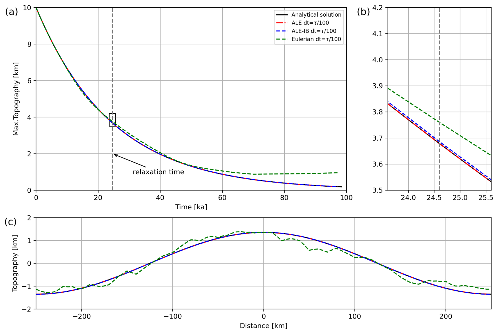
Figure 4 (a) Maximum topography of the models in Experiment 1 over time, shown from the analytical solution (black line) and from free-surface simulations using three different schemes: ALE (magenta dash-dotted line), ALE-IB (blue dashed line), and Eulerian (teal dashed line). (b) Zoomed-in view of the area in (a). (c) Topography at $\text{Time}=\mathrm{2}{t}^{*}$.

When the free surface is not explicitly tracked using additional tracers, the surface becomes unidentifiable, as shown in Fig. 1e. In such cases, the surface must be tracked via particles representing the top of the solid or the interface between rock and air, or through an averaged interface based on volume ratios. Using extra particles to trace the surface, common in this study, often results in a rough interface with undesired spatial fluctuations as discussed in Crameri et al. (2012). These fluctuations arise because the distance between markers and the interface is finite and irregular, leading to small velocity variations during advection.

Such fluctuations can be mitigated by employing finer vertical spacing in the computational mesh or by utilizing marker chains or level-set methods to more accurately assign viscosity and density to nodal points. Another strategy is the volume of fluid method (Gray, 2025), which involves interpolating material types (0=Air, 1=Rocks) from Lagrangian markers to Eulerian mesh nodes using a distance-dependent average. This is followed by computing the position of the topography surface, defined as the isosurface of 0.5, based on the Eulerian nodal material type values. The ALE-IB scheme introduced here provides an alternative way to inherently suppress these fluctuations, achieving accuracy comparable to the ALE scheme while maintaining robust surface tracking.

Additionally, the convergence of the Stokes solver within the ALE and ALE-IB scheme with the FSSA (see Eq. 9), as well as in all schemes without the FSSA, was tested over a range of time steps. This was assessed using the L²-norm of the error in the topography at $\text{Time}=\mathrm{2}{t}^{*}$ from the numerical modelling compared to the analytical solution. The convergence study involved a sequence of seven time steps: $[\mathrm{1},\mathrm{1}/\mathrm{2},\mathrm{1}/\mathrm{4},\mathrm{1}/\mathrm{8},\mathrm{1}/\mathrm{16},\mathrm{1}/\mathrm{32},\mathrm{1}/\mathrm{64}]t^{*}$. Figure 5 illustrates how the FSSA effectively reduces topography errors even at relatively larger time steps. When using FSSA, both ALE and ALE-IB achieve relatively small errors. It is important to note that FSSA introduces a conditional time step constraint. Therefore, we recommend using it primarily when calculations have to be performed with large time steps.

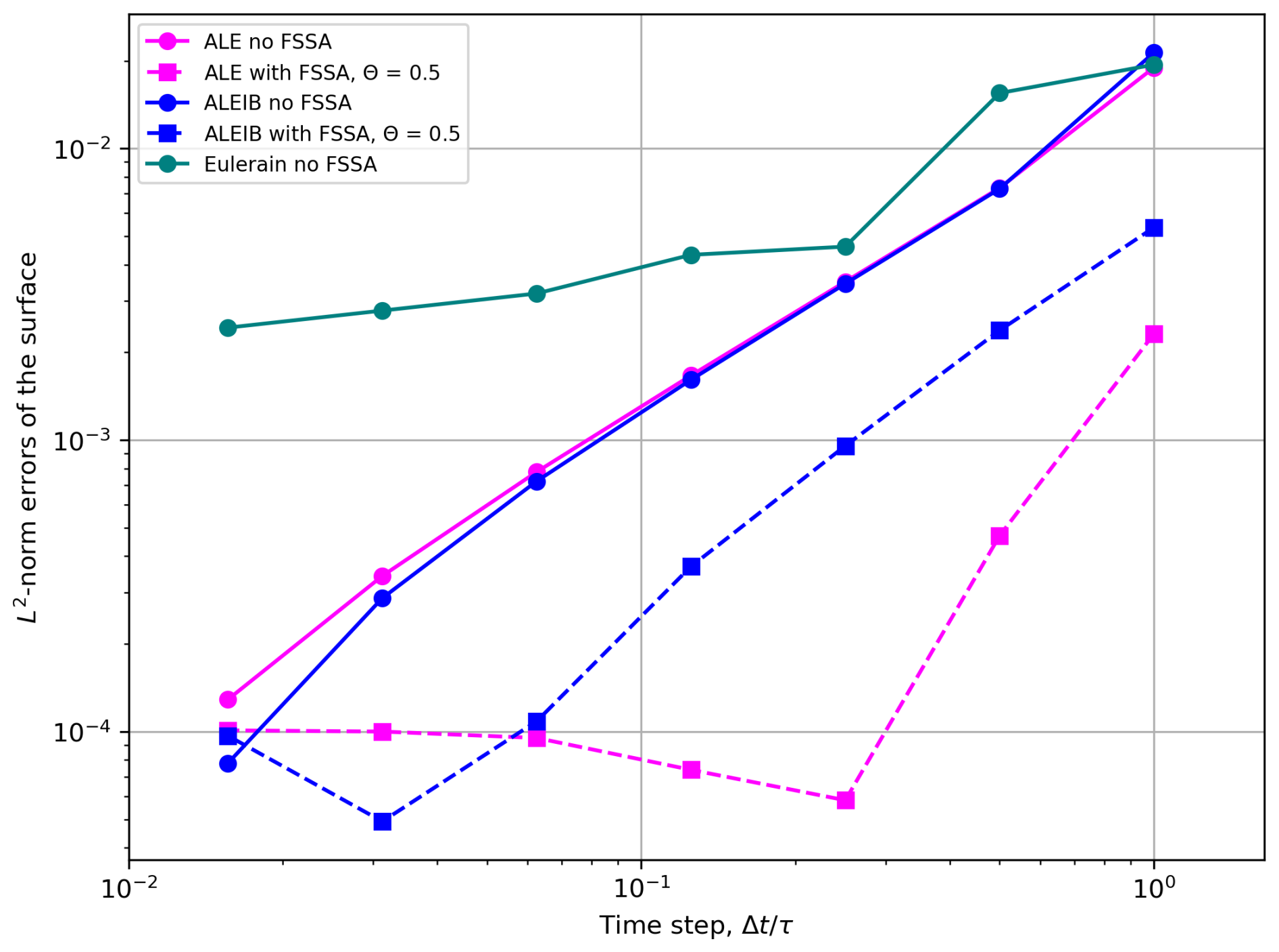
Figure 5 Convergence errors of the free surface simulations with FSSA over different time steps Δt.

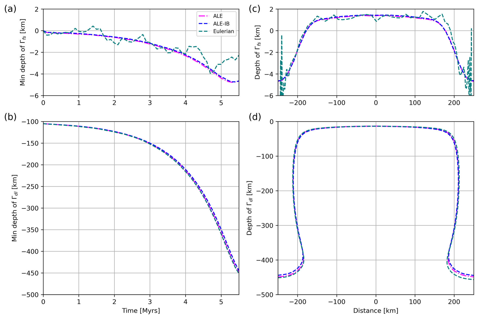
Figure 6 (a) Minimum depth of the surface Γ_fs in Experiment 2 over time, shown from free-surface simulations using three different schemes: ALE (magenta dash-dotted line), ALE-IB (blue dashed line), and Eulerian (teal dashed line). (b) The elevation of Γ_fs over x distance. (c) Minimum depth of the lithosphere/asthenosphere interface Γ_dl, (d) The depth of the interface Γ_dl.

5.2 Rayleigh–Taylor instability

Following the methodologies outlined in Kaus et al. (2010) and Duretz et al. (2011), we continuously monitored the evolution of the lithosphere-asthenosphere interface, defined here as the boundary between denser and less dense materials, and tracked the position of the free surface over time. The results (shown in Fig. 6b), demonstrate that all three simulation schemes: ALE, ALE-IB, and Eulerian are capable of accurately reproducing the results reported in Kaus et al. (2010) when employing sufficiently small time steps. Notably, the time step used in these simulations is smaller than the Courant criterion, fixed at 2.5 ka, to prevent numerical instabilities such as the “drunken sailor” oscillations commonly encountered in free surface simulations. Both the ALE and ALE-IB schemes exhibit excellent agreement in tracking the evolution of the interfaces and the free surface. In contrast, the Eulerian scheme displays significant fluctuations in both the free surface and the lithosphere/asthenosphere interface, along with asymmetric features, especially in the interface's depth profile (Fig. 6d).

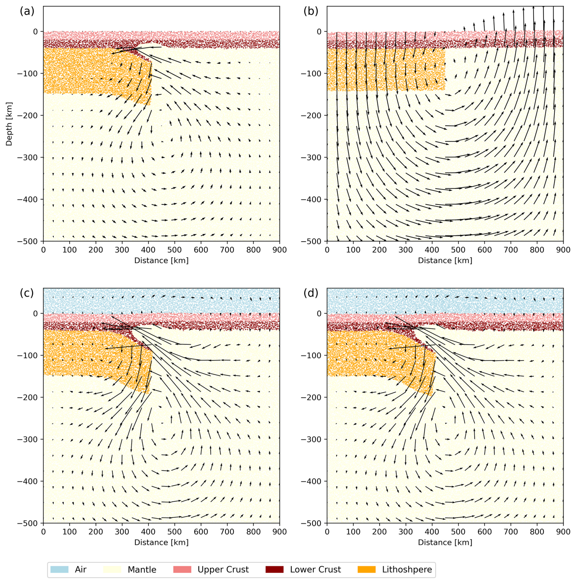
Figure 7 Experiment 3: (a) free slip in Eulerian scheme, Time=4 Ma, (b) free surface in ALE scheme, Time=500 year, (c) free surface in ALE-IB scheme, Time=4 Ma, (d) free surface in Eulerian scheme, Time=4 Ma.

The fluctuations observed in the Eulerian approach are likely attributable to the inherent numerical diffusion and irregularities associated with fixed-grid advection, which can cause the interface to oscillate and distort over time. Conversely, the ALE and ALE-IB schemes, with their moving mesh and improved interface tracking strategies, maintain more stable and physically consistent interface evolutions, underscoring their robustness for long-term geodynamic simulations.

5.3 Delamination

For the chosen model configuration, delamination of the denser lithosphere occurs progressively over time. Comparing the model from Beall et al. (2017) with a free-slip boundary condition at the top, the free-surface simulations within the ALE-IB and Eulerian schemes exhibit relatively faster delamination (Fig. 7a, c, and d). In this context, the free-slip top boundary can be interpreted as a very rigid layer over the upper crust, whereas the free surface in the ALE schemes effectively represents a weak, deformable upper boundary.

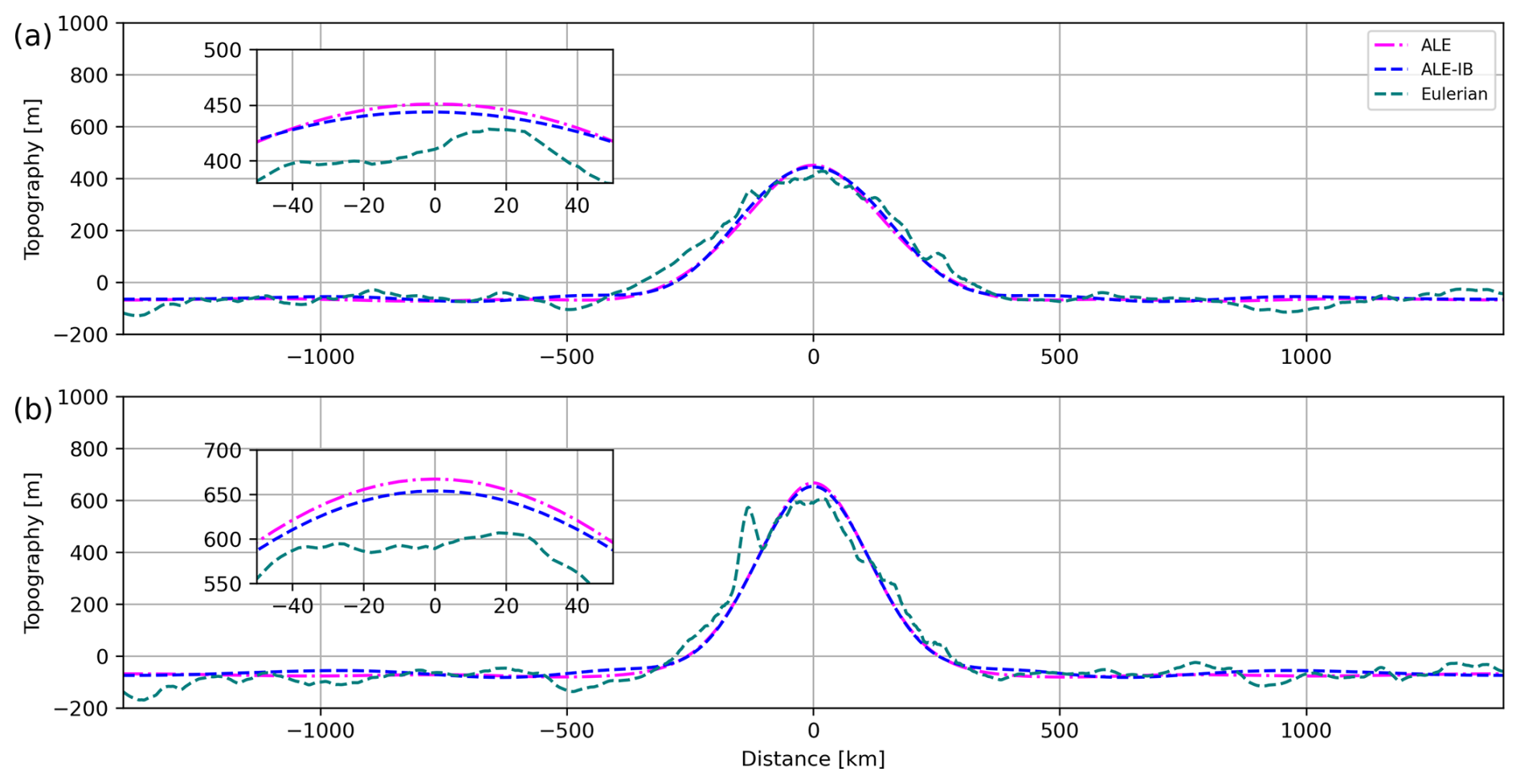
Figure 8 (a) Topography in Experiment 4, shown from free-surface simulations using three different schemes: ALE (magenta dash-dotted line), ALE-IB (blue dashed line), and Eulerian (teal dashed line) at Time=4 Ma. (b) Topography at Time=8 Ma.

However, the ALE scheme exhibits strong counter-clockwise deformation patterns, even with small time steps, primarily due to asymmetry in the model geometry. This is particularly evident with the presence of a denser lithosphere confined to one half of the domain (see Fig. 7b). In contrast, the ALE-IB scheme offers advantages over the traditional ALE approach in such scenarios, providing more stable simulations of free-surface evolution when dealing with asymmetric geometries. Similar cases are discussed in Gerya (2019), where slab bending is triggered by asymmetrical lithospheric thicknesses. Additionally, in models requiring an open bottom boundary, the ALE-IB and Eulerian schemes with a free-slip top boundary condition over the sticky air layer can handle such situations more effectively, whereas the standard ALE scheme tends to exhibit strong numerical instabilities under these conditions.

5.4 Rising Sphere

In the rising sphere model, the plume ascends and approaches the lithosphere over time. Figure 8 displays the surface topography at 4 and 8 Ma. The results from the ALE and ALE-IB schemes remain in good agreement with each other, demonstrating consistent plume evolution and corresponding topographic signals. In contrast, the Eulerian method exhibits strong fluctuations, with the topography reaching approximately a 7 % difference compared to the ALE and ALE-IB results.

5.5 Subduction

The topography generated by the ALE-IB and ALE schemes is similar, displaying smooth and physically plausible surface features. In contrast, the Eulerian scheme produces a basin with a sharper angle on the left side of the island arc, resulting in less realistic surface morphology. Our ALE and ALE-IB scheme results are more comparable to the free-surface case in the Eulerian scheme reported in Crameri et al. (2017), as illustrated in their Fig. 4, where a shape-function averaging method was employed in Eulerian staggered grid scheme on all the uppermost rock tracers and the lowermost air tracers. This approach, combined with the sticky air method, yields more accurate surface representations than the pure Eulerian scheme we used here.

The ALE-IB scheme can produce realistic, single-sided subduction features similar to those obtained with the shape-function averaging method. It also achieves reasonably accurate topography and effectively overcomes mesh distortion issues common in the standard ALE scheme (see Fig. 9a). This demonstrates that our approach not only maintains topographic accuracy but also enhances numerical stability during complex subduction simulations.

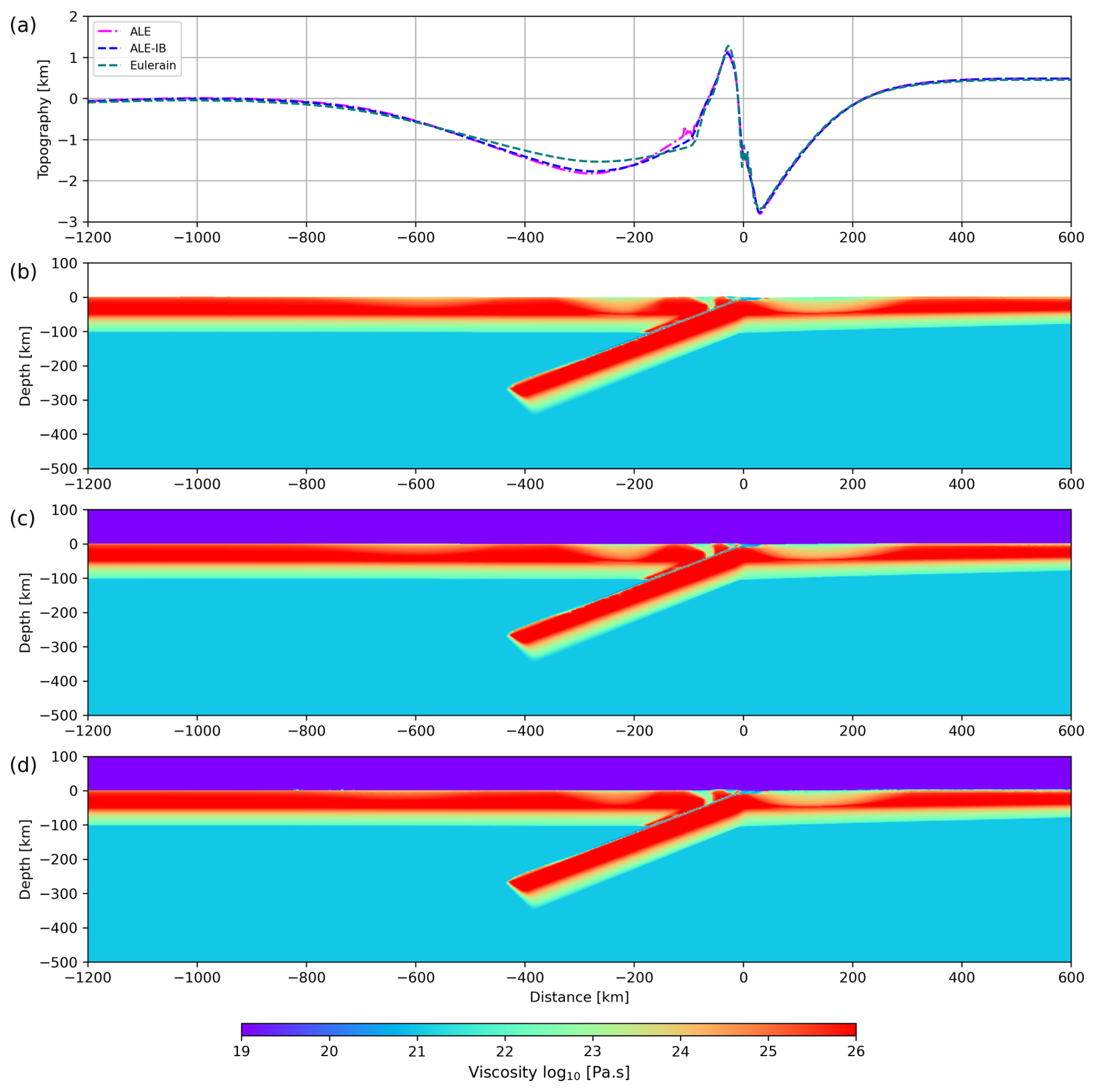
Figure 9 (a) Topography in Experiment 5 over time, shown from free-surface simulations using three different schemes: ALE (magenta dash-dotted line), ALE-IB (blue dashed line), and Eulerian (teal dotted line) at Time=1.6 Ma. (b–d) Viscosity field in ALE, ALE-IB, and Eulerian scheme respectively, at Time=1.6 Ma.

5.6 Model limitations

While the proposed ALE-IB scheme offers significant advancements in simulating true free surface dynamics, several limitations should be acknowledged:

1. Computational cost: Although the internal boundary approach reduces certain numerical artifacts, it introduces additional complexity in mesh management and boundary condition implementation. This can result in increased computational expense, particularly for large-scale or high-resolution simulations.

2. Approximate surface conditions: Although the internal boundary method effectively emulates a true free surface, the boundary conditions employed remain approximations. They may not fully capture the complex interactions between Earth's surface and the atmosphere or hydrosphere, necessitating further integration of surface process coupling to improve realism.

3. Mesh elements type: In our experiments, most models utilized meshes with Q₁dQ₀ elements. However, as demonstrated in Thieulot and Bangerth (2022), Q₁dQ₀ elements tend to be unstable and inaccurate in practice. Consequently, we believe that higher-order elements such as Q₂Q₁ and Q₂P₋₁ offer more robust and reliable options for geodynamic simulations (see Fig. A1), despite their increased implementation complexity and higher computational costs associated with solving the resulting linear systems. Underworld 2 supports high-order discretizations like Q₂Q₁ and Q₂P₋₁. Underworld 3 extends this support to additional high-order discretizations, making it well-suited for the ALE-IB scheme, though further testing is needed.

Future research should focus on optimizing mesh management algorithms, incorporating more comprehensive physical processes, and validating results against observational data. These steps are essential for enhancing the applicability, accuracy, and overall robustness of this scheme in realistic geodynamic modelling.

6 Conclusions

We propose a novel scheme called ALE-IB, which enhances the traditional ALE framework by incorporating an internal boundary to simulate the true free surface in geodynamic models. This approach enables comprehensive domain calculations and the flexibility to apply additional boundary conditions directly to the free surface as needed. To evaluate its applicability and benefits, we conducted five numerical experiments comparing the free surface simulations across three different schemes: (a) ALE, (b) ALE-IB, and (c) Eulerian.

The results demonstrate that the ALE-IB scheme achieves accuracy comparable to the traditional ALE method and effectively overcomes the marker fluctuation issues associated with the “sticky air” layer in particle-in-cell approaches within the Eulerian scheme. Unlike the standard ALE, which can suffer from mesh distortion and instability in complex and asymmetric geometries, the ALE-IB consistently maintains stable and realistic surface evolution, even in challenging scenarios such as large asymmetric deformations. The ALE-IB scheme can accurately capture surface topography, interface evolution, and subduction processes.

Overall, our findings highlight that the ALE-IB scheme not only matches the accuracy of existing methods but also offers significant advantages in stability, robustness, and physical realism. Consequently, it presents a promising alternative to conventional ALE and “sticky air” techniques in the Eulerian scheme, particularly for multi-material near free surface systems and surface process modelling, where precise and stable free surface representation is crucial. This framework paves the way for more reliable and versatile geodynamic simulations, advancing our understanding of Earth's lithospheric and mantle dynamics with a true free surface.

Appendix A: Higher-order mesh elements test

Here we present the results from Experiment 1, which explores the impact of different mesh element types on accuracy. Higher-order elements such as Q₂Q₁ and Q₂P₋₁ significantly improve accuracy for both the ALE-IB and Eulerian schemes. These elements enable more precise modeling results (see Fig. A1). The Eulerian scheme using the Q₂P₋₁ elements achieves accuracy comparable to the ALE-IB scheme with the Q₁dQ₀ elements. Furthermore, the ALE-IB scheme, when utilizing Q₂Q₁ and Q₂P₋₁ elements, exhibits accuracy close to that of the ALE scheme with the Q₁dQ₀ elements, which closely aligns with the analytical solution. This demonstrates the effectiveness of higher-order elements in enhancing the precision of simulations, emphasizing their utility in applications requiring high accuracy.

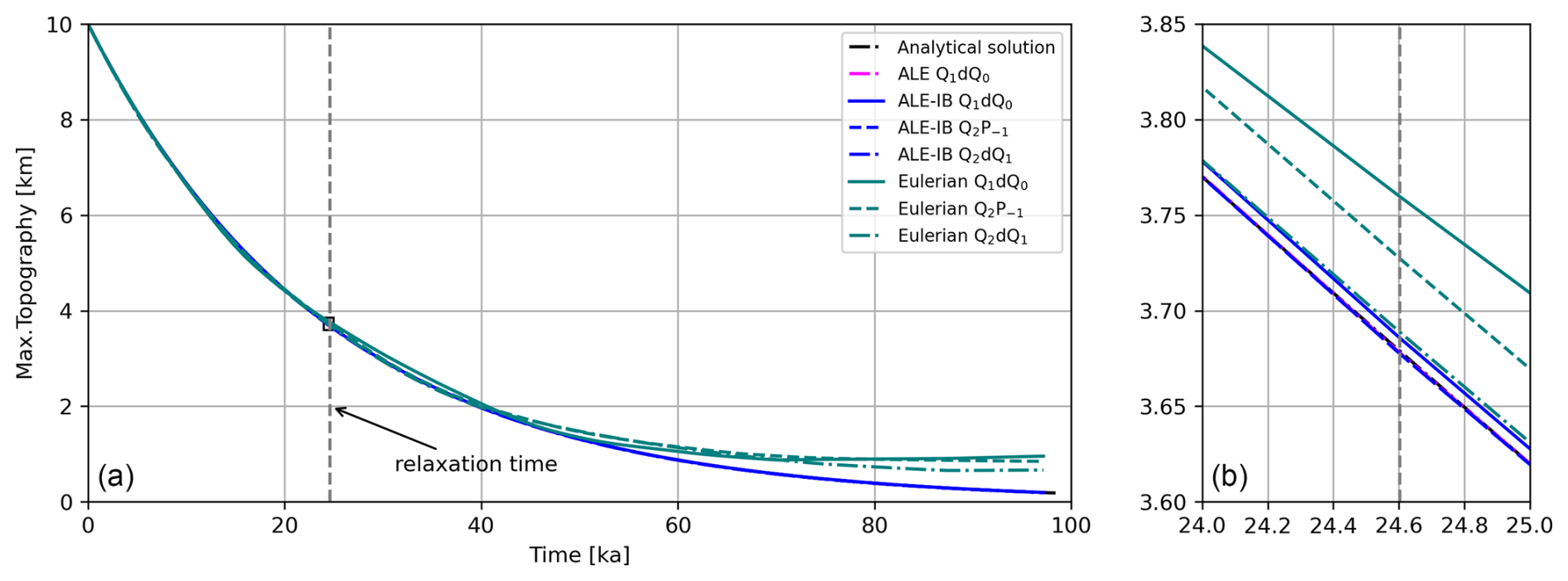
Figure A1 (a) Maximum topography of the models in Experiment 1 over time, shown from the analytical solution (black line) and from free-surface simulations using three different schemes with different mesh element type: ALE with Q₁Q₀ elements; ALE-IB with Q₁Q₀, Q₂Q₁, and Q₂P₋₁ elements; Eulerian with Q₁Q₀, Q₂Q₁, and Q₂P₋₁ elements. (b) Zoomed-in view of the area in (a).