TREED (v1.0): a trait- and optimality-based eco-evolutionary vegetation model for the deep past and the present

We present the TREED model (TRait Ecology and Evolution over Deep time), a trait- and optimality-based vegetation model to simulate vegetation structure, carbon cycling and eco-evolutionary adaptation dynamics to climate and CO₂ changes across geologic time scales. The global grid-based vegetation model represents plant carbon allocation and trait evolution as a set of carbon economic trade-offs. Based on optimality principles, it is assumed that functional traits of the modelled community-representative average plants evolve towards an optimum that maximizes height growth while maintaining a positive carbon balance. The considered trait trade-offs resolve potential plant height, leaf carbon pool size, leaf longevity, and phenology as the major axes of plant trait variation. Based on these key traits, whole-plant structure and functioning are derived using functional and allometric relationships. In its eco-evolutionary mode, vegetation-mediated carbon cycling can be tracked over the course of climatic transitions, testing the effects of the speed of evolutionary trait adaptation and dispersal dynamics. Moreover, with its generalized plant physiology, continuous trait space, and lack of pre-defined functional types, the model can be used to calculate metrics of biodiversity, including indices of functional diversity and species richness potential. With a low computational demand, a flexible time stepping scheme and scalable adaptation parameters, TREED is intended to simulate biological and environmental transitions across time scales spanning from centuries to millions of years. Here, we present the underlying theory and model functions and evaluate model outputs against present-day observations. We show that the trait- and optimality-based approach captures major patterns in present-day vegetation-mediated carbon and water fluxes, biomass carbon storage, vegetation height, leaf traits, as well as the global distribution of plant biodiversity. Finally, we illustrate its application in the context of paleoclimate and palaeoecological research using the Paleocene-Eocene Thermal Maximum as a case study, showing how eco-evolutionary adaptation dynamics of vegetation may strongly affect global carbon cycle dynamics during hyperthermal events. The TREED model is a step towards a more self-consistent and parameter-scarce representation of vegetation dynamics under environmental conditions that are fundamentally different from the present. In combination with geochemical and paleobotanical data, the model may help to better constrain the resilience of vegetation-mediated Earth system functions to perturbations in the geologic past and at present.

1 Introduction

Since the emergence of plants on land, vegetation has played a fundamental role in the functioning of the Earth system, controlling the cycling of carbon, oxygen, water and energy on timescales ranging from seconds to millions of years. On short timescales, vegetation-climate interactions include biophysical interactions with the atmosphere, such as the exchange of energy, momentum and water (Boyce and Lee, 2017), or the assimilation and sequestration of carbon in biomass and soils (Sitch et al., 2008). On geologic timescales of millions of years, vegetation interacts with continental erosion and weathering processes, and contributes to the burial of organic material in marine sediments, representing long-term controls of Earth's climate evolution, atmospheric composition and surface structures (Berner, 2004; Dahl and Arens, 2020; Hilton and West, 2020). While controlling the functioning of global biogeochemical cycles, vegetation systems are at the same time highly sensitive to changes in the physical environment. To a certain degree of environmental change, plants can respond through acclimation and variation in the expression of plastic traits (Kristensen et al., 2020; Liu et al., 2024; Wang et al., 2020). More severe and persistent perturbations can trigger large-scale eco-evolutionary dynamics, including range shifts of species tracking their habitats, competition dynamics, and trait evolution due to the continuous selection for individuals that are best adapted to the new conditions (Korasidis et al., 2022; Matthaeus et al., 2023; McElwain et al., 2007; Sitch et al., 2008; Wing et al., 2005). The physical environment and vegetation represent a co-evolutionary system through time. Understanding their dynamic interplay is key to resolving Earth's past and future bioclimatic evolution (Beerling and Berner, 2005; Gurung et al., 2024).

The paleobotanical record offers several examples of how vegetation diversity and functioning have markedly changed during past periods of climatic change (Korasidis et al., 2022; McElwain and Punyasena, 2007; Wing and Currano, 2013; Xu et al., 2022), and similar dynamics are expected under current anthropogenically driven climate change (Etterson and Shaw, 2001; Gonzalez et al., 2010; Sitch et al., 2008). Due to the scarcity of observational data from the deep past, and in order to project how land surface processes and climate will interact in the future, we generally rely on numerical models to simulate the behaviour and interactions between vegetation and other Earth system components (Fisher et al., 2014; Matthaeus et al., 2023; McElwain et al., 2024). Complex models exist to describe communities of plant species and associated biogeochemical and ecological processes (i.e., dynamic vegetation models), which have been fundamental to advancing our understanding of vegetation and climate interactions under global environmental change (Fisher et al., 2014; Sitch et al., 2008). An important drawback of most currently available vegetation models is that they are strongly parametrized around the functioning of plant species and communities under present-day environmental conditions. For example, most dynamic vegetation models represent the global diversity of plant species with a small and fixed number of plant functional types that differ in pre-defined functional traits and biogeochemical parametrizations (Berzaghi et al., 2020; Fisher et al., 2014). This approach neglects eco-evolutionary dynamics and natural selection that will result in vegetation systems continuously responding and adapting to new environmental conditions (Berzaghi et al., 2020). The static approach of plant functional type analogues is particularly problematic when applying the models to climatic conditions that are fundamentally different from the present, as is the case for most of Earth's past (Judd et al., 2024), or as we expect under future warmer climates (Fisher et al., 2014; Franklin et al., 2020). It is similarly problematic during past periods when modern-like plant traits and trait combinations had not yet evolved (Matthaeus et al., 2023; White et al., 2020; Wilson et al., 2017). Moreover, an approach that strongly focuses on present-day functioning will limit our ability to understand major co-evolutionary transitions in Earth's past, during which both biotic and abiotic environmental changes interactively reshaped the functioning of the Earth system.

A promising approach to increase robustness in the prediction of vegetation functioning under changing environmental conditions is to focus on organizing principles of biological systems (Franklin et al., 2020; Harrison et al., 2021). An organizing principle describes how components of a complex system behave together, rather than characterizing the functioning of the individual components. Natural selection, i.e., the differential survival and reproduction success of individuals in a specific environment, represents such an organizing principle for vegetation systems. All plants that can persist in an environment must have traits that allow them to pass through the filter of natural selection, with abiotic and biotic selection processes eliminating uncompetitive plants. Consequently, trait-environment relationships may be predictable by considering selection to favour plant functional trait combinations that maximize fitness (Franklin et al., 2020; Harrison et al., 2021). Model-based implementations of such eco-evolutionary optimality concepts make use of plant carbon economics with trait and allocation strategies being associated with carbon gains and losses that apply across species. By maximizing a fitness measure, an optimal trait allocation strategy under given environmental conditions can be predicted (Franklin et al., 2020). The two major axes of variation in plant growth forms observed across the globe today include variation in plant size and leaf characteristics (Díaz et al., 2016). Both these functional traits are strongly associated with a plant's carbon balance. Height growth determines the competitiveness in acquiring light resources for carbon assimilation, but is associated with increased construction and maintenance carbon losses (Falster and Westoby, 2003). Variation in leaf characteristics particularly represent the leaf economics spectrum, ranging from species with economically constructed and short-lived “acquisitive” leaves of low leaf mass per area, to species with “conservative” leaves that have longer lifespans and increased persistence under environmental stress but are associated with a reduced carbon sequestration potential (Díaz et al., 2016; Wright et al., 2004). Mechanistic modelling of such carbon economic trade-offs across environmental gradients can resolve major patterns in the global vegetation trait distribution (Franklin et al., 2014, 2020; King, 1990; Rüger et al., 2020; Schymanski et al., 2009; Wang et al., 2023).

Here, we present and evaluate the model TREED (TRait Ecology and Evolution over Deep time), a vegetation model to continuously predict vegetation structure and functioning based on eco-evolutionary optimality principles across timescales from centuries to millions of years. The grid-based vegetation model is built around competing trait allocation strategies that determine plant fitness under given environmental conditions. It is assumed that adaptation, competition, environmental filtering and evolution result in plants to allocate carbon and express traits in a way that maximizes height growth (i.e., light competitiveness), while maintaining a positive carbon balance (necessary condition to survive). With the current set of considered trait trade-offs, the model resolves plant height, leaf longevity, leaf carbon, and phenology (deciduous or evergreen) as the main independent axes of vegetation trait variation. Additional traits and whole-plant architecture are derived using functional and allometric relationships with these main traits, and by considering a generalized plant physiology. With a low model complexity, minimal necessary environmental inputs, and fast computational time, the model is primarily designed to investigate vegetation dynamics in Earth's past and to test a range of eco-evolutionary hypotheses during periods of environmental change. We will describe and evaluate the following main functionalities of the model:

1. Predict the global vegetation structure, trait distribution, and associated carbon fluxes of a vegetation in eco-evolutionary equilibrium with the environment.

2. Predict vegetation structures and functioning during climatic transitions, limited by the capacity of vegetation to adapt traits through evolution or a dispersal-based vegetation redistribution.

Finally, testing the fitness of different functional trait combinations in an environment–as done in TREED–is strongly related to the concept of functional diversity, i.e., the range of functional traits that can be observed within a plant community. Using the generalized plant physiology and continuous trait space of the model, we use it to:

• 3.

  Identify locations of a high potential for functional richness and co-existence of variable plant trait combinations. By combining local functional richness and vegetation diversity metrics at the landscape level, we further estimate locations of a high plant biodiversity potential.

2 TREED model description

A TREED model simulation consists of four processes executed in succession (Fig. 1a): (1) initialization and allocation of plant functional traits, (2) calculation of carbon and water fluxes, (3) an optimization function to predict the optimal trait distribution under given climatic and topographic conditions, and (4) eco-evolutionary processes including trait evolution and dispersal dynamics that determine the transition speed from a prevailing vegetation trait distribution towards the predicted optimum trait distribution.

TREED is a grid-based vegetation model: every grid cell is associated with a combination of traits that describe a location's vegetation structure. As the model does not explicitly resolve plant individuals or populations within the grid cell, the trait values can be considered to describe a community-representative average plant that occupies the entire grid cell. Four key traits fundamentally describe a location's vegetation structure: an individual plant's average leaf carbon pool size during the growing season (C_leaf; g C per individual), the community-average plant height (H; m), the dominant phenological strategy (phenology; deciduous or evergreen) and the average leaf longevity (a_ll; years). Additionally, the vegetation of each location is associated with a climatic niche that describes bioclimatic limits for productivity. The climatic niche is only considered in transient simulations as described in Sect. 2.4. Based on these key traits and generalized allometric and functional relationships, a range of additional plant characteristics important for vegetation functioning are derived. In each location, the values of the key traits are determined simultaneously in an optimization procedure under consideration of local climatic conditions, searching for the trait combination that maximizes the community average plant height under the constraint of maintaining a positive annual carbon balance (balance between photosynthesis, respiration and tissue turnover carbon investments). Functional trait trade-offs thereby limit the possible trait space to a realistic range. By maximizing the average plant height, the model assumes that plants are in continuous competition for light and that plant trait combinations that maximize photosynthetic carbon gains and height represent stable trait strategies that are likely to persist and dominate an ecosystem, as explained in more details in Sect. 2.3–2.4.

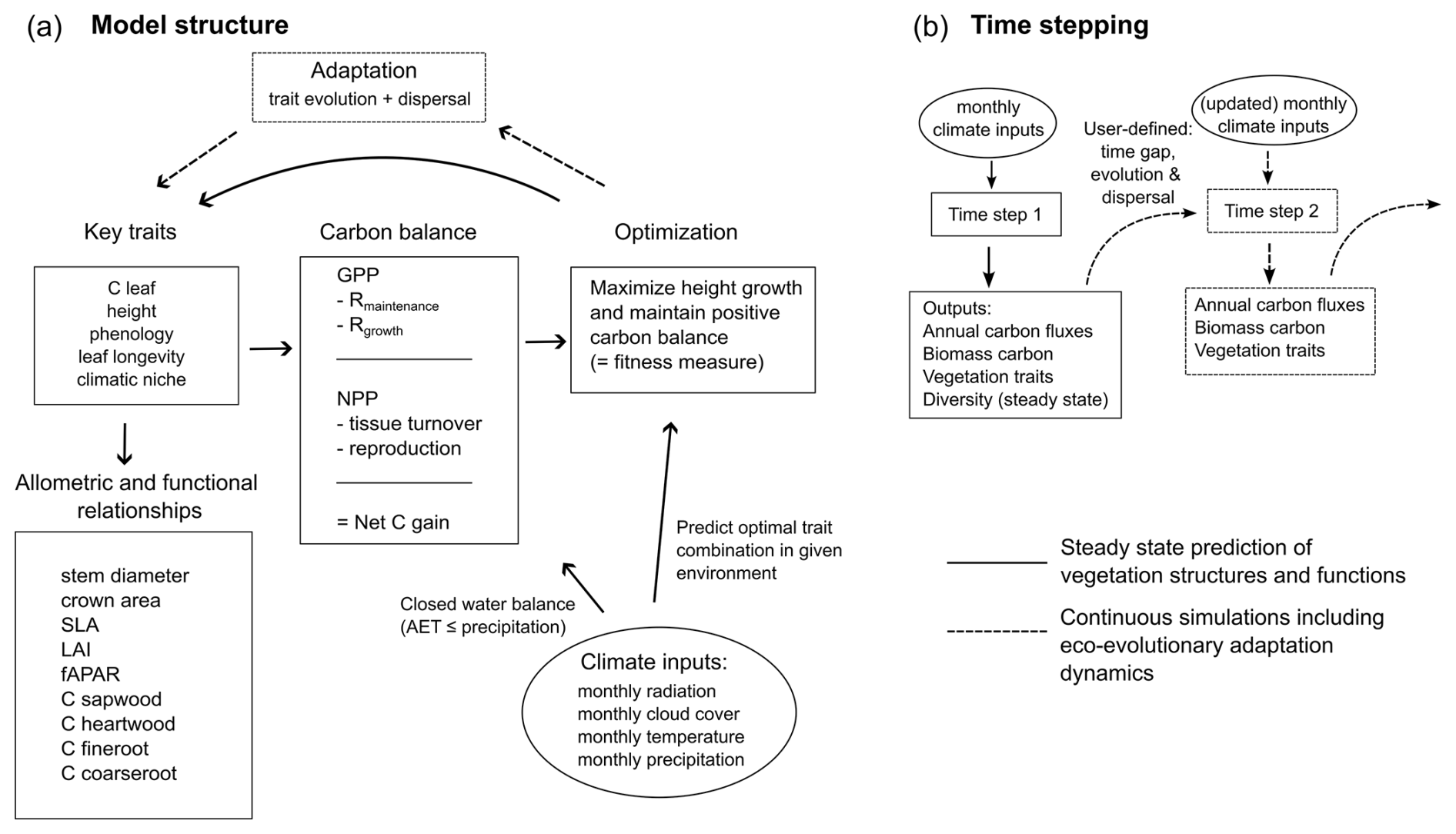
Figure 1 Schematic overview of TREED model processes. (a) Overview of model steps. Squares indicate model processes and variables tracked in the model; rounds indicate external climate inputs. Continuous arrows represent steps considered in a steady state simulation; dashed arrows indicate optionalsteps in a continuous, non-steady state simulation considering eco-evolutionary adaptation dynamics. Key traits determine plant structures, carbon and water fluxes. Using an optimization procedure, for each climatic environment an optimal trait combination is evaluated that maximises the community-average vegetation height while maintaining a positive carbon balance. The optimum trait combination is used to approximate vegetation functioning in the steady state mode and serves as a target for eco-evolutionary adaptation dynamics. Abbreviations: C = carbon, SLA = specific leaf area, LAI = leaf area index, fAPAR = fraction of absorbed photosynthetically active radiation, GPP = gross primary productivity, AET = actual evapotranspiration, R_maintenance= maintenance respiration, R_growth= growth respiration, NPP = net primary productivity. (b) Time stepping in the TREED model. The model calculates annual carbon fluxes, biomass carbon storage and biodiversity indices using monthly climate inputs. In the model's eco-evolutionary mode, dispersal- and evolution-based trait changes across a user-defined time gap can be simulated. Diversity indices are only calculated in steady state mode assuming optimal adaptation, not considering dispersal and evolution dynamics.

2.1 Allometric and functional relationships

Specific leaf area (SLA; m² g C⁻¹) is related to leaf longevity, representing the leaf economics spectrum (Wright et al., 2004). Plants across growth forms, biomes and climates show a similar range of feasible leaf investment strategies along a gradient from “acquisitive” leaves with high SLA but low leaf longevities, to “conservative” leaves with low SLA but increased leaf longevity and persistence in harsh environments (Díaz et al., 2016; Wright et al., 2004). The generalized functional relationship used in the TREED model represents an intermediate form of the leaf economic trade-off used for needle-leaved and broadleaved plants with prescribed leaf longevities in the LPJ dynamic vegetation model (Schaphoff et al., 2018; Fig. 2):

$$\begin{array}{}\text{(1)}& \mathrm{SLA}=\left(\mathrm{2}\times {\mathrm{10}}^{-\mathrm{4}}\right)\cdot {\displaystyle \frac{\mathrm{1}}{{\mathrm{DM}}_{\mathrm{c}}}}\times {\mathrm{10}}^{\mathrm{2.25}-\log \left(a_{\mathrm{ll}}\cdot \mathrm{12}\right)}\end{array}$$

with DM_c being an assumed average dry matter carbon content of 0.47 g C per g of dry matter and a_ll the leaf longevity in years. The generalized relationship implies that modelled plants will have leaf longevity and SLA combinations in between two endmember strategies: short leaf longevity/high SLA strategies, representing broadleaved deciduous or evergreen plants, or long leaf longevity/low SLA representing evergreen, needle-leaved plants (Fig.  2). For a given leaf carbon pool, a high SLA will result in a high leaf area and light interception potential but is associated with high annual carbon investments to rebuild the leaf carbon pool due to the short leaf longevity. Whether such a strategy is favourable over long leaf longevities and reduced annual leaf carbon investments, as well as the exact duration of the leaf longevity, depend on local climatic conditions (precipitation, radiation and temperature) and is evaluated in the optimization procedure (see Sect. 2.3). By affecting the carbon assimilation potential as well as annual carbon turnover costs, the leaf investment trade-off further contributes to determine whether an evergreen or a deciduous phenology (i.e., no leaves during part of the year) is more favourable under temperate climatic conditions (see Sect. 2.2.3). The consideration of a predicted and continuous range of possible leaf longevities and SLA strategies represents an important difference to plant functional type-based vegetation models with prescribed leaf traits.

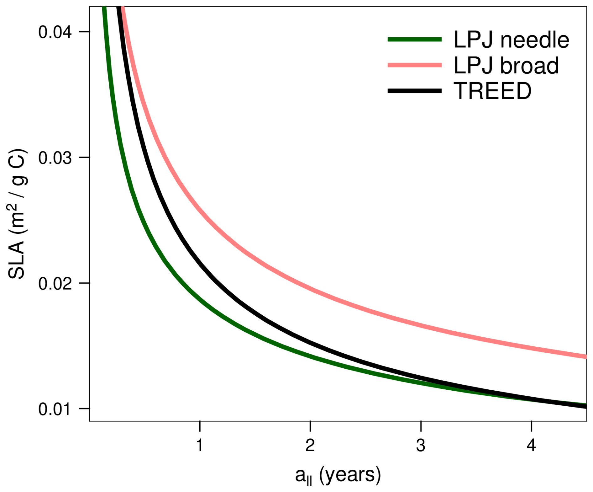
Figure 2 Generalized relationship between leaf longevity (a_ll) and specific leaf area (SLA). For a given size of the leaf carbon pool, short leaf longevities and high SLA result in a high light interception potential (e.g., total leaf area and leaf area index) but are associated with higher annual carbon investments to rebuild the carbon pool due to the short longevity. The generalized relationship employed in the model represents an intermediate form between the leaf longevity to SLA relationships considered for specific plant functional types with fixed a_ll in the LPJ vegetation model (Schaphoff et al., 2018; Sitch et al., 2003).

Following the allometric scaling relationships from the LPJ vegetation model (Schaphoff et al., 2018; Sitch et al., 2003), the size of a plant individual's average leaf carbon pool (C_leaf) and SLA determine the average leaf area of a plant (LA; m²):

$$\begin{array}{}\text{(2)}& \mathrm{LA}=\mathrm{SLA}\cdot C_{\mathrm{leaf}}\end{array}$$

Following the pipe model (Shinozaki et al., 1964; Waring et al., 1982), an individual's leaf area and sapwood cross-section area (SA; m²) are assumed proportional (all pre-defined model parameters are listed in Table 1):

$$\begin{array}{}\text{(3)}& \mathrm{LA}=k_{\mathrm{la}:\mathrm{sa}}\cdot \mathrm{SA}\end{array}$$

Leaf and fine root carbon allocation (C_fineroot; g C per individual) are related by a fine root to leaf carbon ratio (r:s; dimensionless):

$$\begin{array}{}\text{(4)}& C_{\mathrm{leaf}}=r:s\cdot C_{\mathrm{fineroot}}\end{array}$$

Plant height and diameter (D; m) are assumed to relate according to (Huang et al., 1992):

$$\begin{array}{}\text{(5)}& H=k_{\mathrm{allom}\mathrm{2}}\cdot D^{k_{\mathrm{allom}\mathrm{3}}}\end{array}$$

Further, diameter and crown area (CA; m²) are assumed to scale following:

$$\begin{array}{}\text{(6)}& \mathrm{CA}=min\left(k_{\mathrm{allom}\mathrm{1}}\cdot D^{k_{\mathrm{rp}}},{\mathrm{CA}}_{\max }\right)\end{array}$$

with an assumed maximum crown area (CA_max) of 15 m² (Sitch et al., 2003). The CA represents the average surface area occupied by a single average plant in a model grid cell.

An average plant's individual leaf area index (LAI_individual; m² m⁻²) can be calculated as:

$$\begin{array}{}\text{(7)}& {\mathrm{LAI}}_{\mathrm{individual}}={\displaystyle \frac{C_{\mathrm{leaf}}\cdot \mathrm{SLA}}{\mathrm{CA}}}\end{array}$$

It is assumed that grid cells are fully covered by the local average plant that is characterised by the five key traits (Fig. 1a). Assuming no canopy overlap, the number of plant individuals per grid cell (N_individuals) is thus $N_{\mathrm{individuals}}=\frac{\text{cell area}}{\mathrm{CA}}.$Consequently, the grid cell's leaf area index (LAI), is equal to the leaf area index of the average individual (LAI = LAI_individual):

$$\begin{array}{}\text{(8)}& \begin{array}{rl}\mathrm{LAI}& ={\displaystyle \frac{{\mathrm{LA}}_{\mathrm{individual}}\cdot N_{\mathrm{individuals}}}{\text{cell area}}}={\displaystyle \frac{{\mathrm{LA}}_{\mathrm{individual}}}{\mathrm{CA}}}\\ & ={\mathrm{LAI}}_{\mathrm{individual}}\end{array}\end{array}$$

The light interception potential within a grid cell, i.e., the fraction of photosynthetically active radiation absorbed by leaves (fAPAR; dimensionless), is estimated using the Lambert-Beer law:

$$\begin{array}{}\text{(9)}& \mathrm{fAPAR}=\mathrm{1}-e^{-k\cdot \mathrm{LAI}}\end{array}$$

Thereby, we account for a tendency of an increased light extinction coefficient (k) for broadleaved, short-lived and high SLA leaves compared to needle-leaved, long-lived and low SLA leaves (Zhang et al., 2014), by linearly relating k in the range between 0.6 and 0.4 to the average leaf longevity, according to:

$$\begin{array}{}\text{(10)}& k=\mathrm{0.6}-\mathrm{0.04}\cdot a_{\mathrm{ll}}\end{array}$$

A plant's sapwood carbon pool (C_sapwood; g C per individual) is derived from the plant's sapwood cross section area and height, assuming a cylindrical geometry and a constant wood density (WD; g C m⁻³):

$$\begin{array}{}\text{(11)}& C_{\mathrm{sapwood}}=\mathrm{SA}\cdot H\cdot \mathrm{WD}\end{array}$$

The model considers a globally generalized plant physiology, and it is therefore assumed that for small plants that would not be considered trees, C_sapwood describes an overall structural carbon pool that is proportional to a plant's height.

Woody tissue represents the by far most important component of global above ground biomass (Brunner and Godbold, 2007). Therefore, a generalized power law derived from global canopy height (Lang et al., 2023) and above ground biomass density estimates (Huang et al., 2021; Santoro et al., 2021) is used to describe the relationship between the modelled volume of an average plant in a grid cell (H⋅ CA) and total stem biomass ($C_{\mathrm{stem}}=C_{\mathrm{sapwood}}+C_{\mathrm{heartwood}}$):

$$\begin{array}{}\text{(12)}& C_{\mathrm{stem}}=k_i\cdot (\mathrm{CA}\cdot H{)}^{k_p}\end{array}$$

Coarse root carbon (C_coarseroot; g C per individual) is assumed to be around a fourth of the stem biomass, as estimated from current above ground and below ground biomass data (Huang et al., 2021):

$$\begin{array}{}\text{(13)}& C_{\mathrm{coarseroot}}=\mathrm{0.25}\cdot \left(C_{\mathrm{heartwood}}+C_{\mathrm{sapwood}}\right)\end{array}$$

All allometric constants ($k_{\mathrm{allom}\mathrm{1}},k_{\mathrm{allom}\mathrm{2}},k_{\mathrm{allom}\mathrm{3}},k_{\mathrm{rp}},k_{\mathrm{la}:\mathrm{sa}}$, k_i, k_p) were calibrated using present-day canopy height and above ground biomass data and are listed in Table 1. In the calibration procedure, we minimized the root mean square error (RMSE) between predicted above ground biomass density, derived using the present-day observed vegetation height and allometric Eqs. (5), (6) and (12), and the observed biomass density from Huang et al. (2021) and Santoro et al. (2021). The resulting height to biomass relationship is outlined in Sect. 5.3 and Fig. 6b.

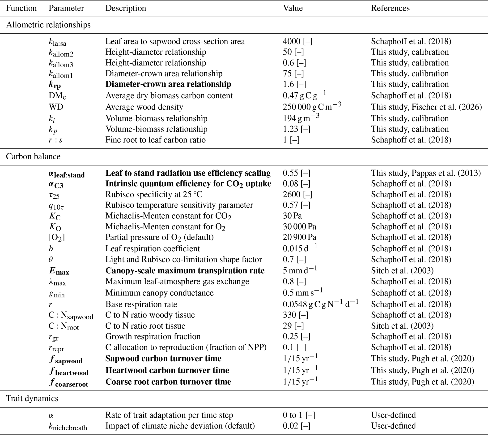
Table 1 Pre-defined TREED model parameters required to approximate vegetation structure, photosynthesis, respiration, carbon turnover and trait evolution. Dimensionless parameters are indicated by [–]. Most parameters are adopted from the Lunt-Potsdam-Jena (LPJ) global dynamic vegetation model family (Schaphoff et al., 2018; Sitch et al., 2003). Allometric constants were calibrated in this study. Parameter values to which model results are expected to be particularly sensitive are marked in bold, following the sensitivity studies of Oberpriller et al. (2022) and Pappas et al. (2013).

2.2 Carbon balance

2.2.1 Photosynthesis and evapotranspiration

Based on the derived characteristics of the vegetation at a location, photosynthetic carbon assimilation, growth and maintenance respiration, and tissue turnover carbon investments are calculated. The following carbon and water flux calculations are adapted from the LPJ vegetation model (Schaphoff et al., 2018; Sitch et al., 2003), with photosynthesis being modelled using the Farquhar photosynthesis model (Farquhar et al., 1980; Farquhar and Caemmerer, 1982) and under consideration of the generalizations for global modelling by Collatz et al. (1991). The “strong optimality” hypothesis (Haxeltine and Prentice, 1996b) is applied, assuming that nitrogen content and Rubisco activity of leaves vary seasonally and with canopy position in a way to maximize the net assimilation at the leaf level. The resulting model has the form of a light-use efficiency model, depending on the photosynthetically active radiation (PAR), temperature, daylength and water availability.

Half of the downwelling shortwave radiation at the surface (RSDS; MJ m⁻² d⁻¹) is assumed photosynthetically active radiation (PAR; MJ m⁻² d⁻¹; Haxeltine and Prentice, 1996a; Schaphoff et al., 2018):

$$\begin{array}{}\text{(14)}& \mathrm{PAR}=\mathrm{0.5}\cdot \mathrm{RSDS}\end{array}$$

The fraction of PAR absorbed by the local vegetation (APAR; MJ m⁻² d⁻¹) is calculated considering a grid cell's fAPAR, a leaf to stand level scaling factor (α_leaf:stand; dimensionless), and a climate niche suitability factor (Φ_nichestress; dimensionless).

$$\begin{array}{}\text{(15)}& \mathrm{APAR}=\mathrm{PAR}\cdot \mathrm{fAPAR}\cdot {\mathit{\alpha }}_{\mathrm{leaf}:\mathrm{stand}}\cdot {\mathrm{\Phi }}_{\mathrm{nichestress}}\end{array}$$

The climate niche suitability factor is an introduced variable that will be described in further detail in Sect. 2.4 and that is only important in non-steady state TREED simulations, considering eco-evolutionary adaptation dynamics between different climate states. The leaf to stand scaling factor accounts for reductions in PAR utilization at the stand level in natural ecosystems (Haxeltine and Prentice, 1996b).

Photosynthesis is calculated as the minimum of light-limited (J_E; mol C m⁻² h⁻¹) and Rubisco-limited photosynthesis (J_C; mol C m⁻² h⁻¹) (Haxeltine and Prentice, 1996a). Light-limited photosynthesis is calculated as:

$$\begin{array}{}\text{(16)}& J_{\mathrm{E}}=C_{\mathrm{1}}\cdot {\displaystyle \frac{\mathrm{APAR}}{\mathrm{daylength}}}\end{array}$$

Where daylength (h) is the number of sunshine hours per day, depending on the day of the year and geographic latitude, and

$$\begin{array}{}\text{(17)}& C_{\mathrm{1}}={\mathit{\alpha }}_{{\mathrm{C}}_{\mathrm{3}}}\cdot f_{\mathrm{temp}}\cdot \left({\displaystyle \frac{p_{\mathrm{i}}-{\mathrm{\Gamma }}_{\ast }}{p_{\mathrm{i}}+\mathrm{2}\cdot {\mathrm{\Gamma }}_{\ast }}}\right)\end{array}$$

With p_i(Pa) being the leaf internal partial pressure of CO₂, calculated as $p_{\mathrm{i}}=\mathit{\lambda }\cdot p_{\mathrm{a}}$, where p_a (Pa) is the ambient partial pressure of CO₂ and λ (dimensionless; between 0 and 0.8) describes the leaf-atmosphere water and carbon exchange. The latter depends on the local water availability and vegetation stomatal opening, determining the concentration ratio between intercellular and ambient CO₂. The ${\mathit{\alpha }}_{{\mathrm{C}}_{\mathrm{3}}}$(dimensionless) in Eq. 17) is the intrinsic quantum efficiency for CO₂ uptake of C₃ plants. In the current model version only C₃ physiology is considered. The factor f_temp (dimensionless) describes a general temperature dependency of the efficiency of the photosynthetic pathway, adapted from Schaphoff et al. (2018) and generalized for all plants as:

$$\begin{array}{}\text{(18)}& {\displaystyle }{f}_{\mathrm{temp},\mathrm{low}}={\displaystyle \frac{\mathrm{1}}{(\mathrm{1}+\exp (\mathrm{0.25}\cdot \left(\mathrm{12}-T\right))}}\text{(19)}& {\displaystyle }{f}_{\mathrm{temp},\mathrm{high}}=\mathrm{1}-{\displaystyle \frac{\mathrm{1}}{\mathrm{1}+\exp (-\left(T-\mathrm{40.85}\right))}}\text{(20)}& {\displaystyle }{f}_{\mathrm{temp}}=f_{\mathrm{temp},\mathrm{low}}\cdot f_{\mathrm{temp},\mathrm{high}}\end{array}$$

with T being the monthly average temperature. Accordingly, f_temp indicates an inhibition of photosynthesis for monthly average temperatures below 0  °C and higher than 45 °C, and an optimum photosynthetic rate between 25–30 °C. Finally, Γ_∗ in Eq. 17) represents the photorespiratory CO₂ compensation point:

$$\begin{array}{}\text{(21)}& {\mathrm{\Gamma }}_{\ast }={\displaystyle \frac{\left[{\mathrm{O}}_{\mathrm{2}}\right]}{\mathrm{2}\cdot \mathit{\tau }}}\end{array}$$

with $\mathit{\tau }={\mathit{\tau }}_{\mathrm{25}}\cdot q_{{\mathrm{10}}_{\mathit{\tau }}}^{\frac{T-\mathrm{25}}{\mathrm{10}}}$ (dimensionless) being the specificity factor that reflects the ability of Rubisco to discriminate between CO₂ and O₂. [O₂] is the partial pressure of oxygen (Pa), τ₂₅ is the τ value at 25 °C, and $q_{{\mathrm{10}}_{\mathit{\tau }}}$ a temperature sensitivity parameter.

The Rubisco-limited photosynthesis is calculated as:

$$\begin{array}{}\text{(22)}& J_{\mathrm{C}}=C_{\mathrm{2}}\cdot V_{\mathrm{m}}\end{array}$$

with

$$\begin{array}{}\text{(23)}& C_{\mathrm{2}}={\displaystyle \frac{p_{\mathrm{i}}-{\mathrm{\Gamma }}_{\ast }}{p_{\mathrm{i}}+K_{\mathrm{C}}\cdot \left(\mathrm{1}+\frac{\left[{\mathrm{O}}_{\mathrm{2}}\right]}{K_{\mathrm{O}}}\right)}}\end{array}$$

where K_C and K_O are Michaelis-Menten constants for CO₂ and O₂, respectively. V_m (mol C m⁻² d⁻¹) represents the maximum Rubisco capacity which is derived from optimizing the daily net photosynthesis at the leaf level with respect to V_m ($\frac{\partial A_{\mathrm{nd}}}{\partial V_{\mathrm{m}}}=\mathrm{0}$, where A_nd=A_gdR_leaf; Haxeltine and Prentice, 1996b) resulting in:

$$\begin{array}{}\text{(24)}& V_{\mathrm{m}}={\displaystyle \frac{\mathrm{1}}{b}}\cdot {\displaystyle \frac{C_{\mathrm{1}}}{C_{\mathrm{2}}}}\cdot \left(\left(\mathrm{2}\cdot \mathit{\theta }-\mathrm{1}\right)\cdot s-\left(\mathrm{2}\cdot \mathit{\theta }\cdot s-C_{\mathrm{2}}\right)\cdot \mathit{\sigma }\right)\cdot \mathrm{APAR}\end{array}$$

where b (d⁻¹) is a static leaf respiration coefficient, θ (dimensionless) a shape parameter that describes the co-limitation of light and Rubisco activity (Haxeltine and Prentice, 1996a), and

$$\begin{array}{}\text{(25)}& {\displaystyle }\mathit{\sigma }=\sqrt{\mathrm{1}-{\displaystyle \frac{C_{\mathrm{2}}-s}{C_{\mathrm{2}}-\mathit{\theta }\cdot s}}}\text{(26)}& {\displaystyle }s={\displaystyle \frac{\mathrm{24}}{\mathrm{daylength}}}\cdot b\end{array}$$

The maximum Rubisco capacity is calculated under the assumption of no water limitation (λ=λ_max).

Daily gross photosynthesis (A_gd; g C m⁻² daytime⁻¹) is calculated as

$$\begin{array}{}\text{(27)}& \begin{array}{rl}{A}_{\mathrm{gd}}& ={\displaystyle \frac{(J_{\mathrm{E}}+J_{\mathrm{C}}-\sqrt{{\left(J_{\mathrm{E}}+J_{\mathrm{C}}\right)}^{\mathrm{2}}-\mathrm{4}\cdot \mathit{\theta }\cdot J_{\mathrm{E}}\cdot J_{\mathrm{C}}})}{\mathrm{2}\cdot \mathit{\theta }}}\\ & \cdot \mathrm{daylength}\end{array}\end{array}$$

Subtracting the daytime leaf respiration results in the daily net daytime photosynthesis (A_dt; g C m⁻² daytime⁻¹):

$$\begin{array}{}\text{(28)}& A_{\mathrm{dt}}=A_{\mathrm{gd}}-\left({\displaystyle \frac{\mathrm{daylength}}{\mathrm{24}}}\right)\cdot R_{\mathrm{leaf}}\end{array}$$

With R_leaf (g C m⁻² d⁻¹) being the leaf dark respiration. Leaf dark respiration is expected to be predominantly driven by the turnover of Rubisco proteins for photosynthesis and thus, closely scales with the maximum Rubisco capacity (Schaphoff et al., 2018; Wang et al., 2020):

$$\begin{array}{}\text{(29)}& R_{\mathrm{leaf}}=V_{\mathrm{m}}\cdot b\end{array}$$

The photosynthetic carbon assimilation rate is related to the canopy conductance of water vapor (g_c; mm s⁻¹) through the CO₂ diffusion gradient between the intercellular airspace and the atmosphere (Schaphoff et al., 2018; Sitch et al., 2003), according to:

$$\begin{array}{}\text{(30)}& g_{\mathrm{c}}={\displaystyle \frac{\mathrm{1.6}\cdot A_{\mathrm{dt}}}{p_{\mathrm{a}}\cdot (\mathrm{1}-\mathit{\lambda })}}+g_{min}\end{array}$$

Where g_min (mm s⁻¹) is a minimum canopy conductance that occurs due to non-photosynthesis related processes. The maximum possible canopy conductance is limited by the local water availability. The exchange of water and carbon with the atmosphere is controlled by the parameter λ, with high λ describing non-water limited conditions and maximum water and carbon exchange, whereas low λ indicates stomatal closure and limited gas exchange. Equation (30) therefore relates stomatal opening, canopy conductance and photosynthetic rate. A potential water limitation is evaluated by comparing the vegetation's water demand (E_demand; mm d⁻¹) with the supply of water, constrained by:

$$\begin{array}{}\text{(31)}& E_{\mathrm{supply}}=\min (E_{\max },P_{\mathrm{mean}})\end{array}$$

where E_max represents a maximum daily canopy-scale transpiration rate of 5 mm d⁻¹ (Sitch et al., 2003), and P_mean is the average daily precipitation rate in mm d⁻¹.

Following Schaphoff et al. (2018) and Monteith (1995), E_demand is calculated as:

$$\begin{array}{}\text{(32)}& E_{\mathrm{demand}}=E_{\mathrm{eq}}\cdot {\displaystyle \frac{{\mathit{\alpha }}_{\mathrm{m}}}{\mathrm{1}+\frac{g_{\mathrm{m}}}{g_{\mathrm{c}}}}}\end{array}$$

Employing a maximum Priestley-Taylor coefficient α_m of 1.391, and a conductance scaling factor g_m of 3.26 mm s⁻¹. E_eq is the equilibrium evapotranspiration rate calculated as:

$$\begin{array}{}\text{(33)}& E_{\mathrm{eq}}={\displaystyle \frac{\mathrm{sa}}{\mathrm{sa}+\mathit{\gamma }}}\cdot {\displaystyle \frac{R_{\mathrm{n}}}{{\mathit{\lambda }}_{\mathrm{vap}}}}\end{array}$$

with sa (Pa K⁻¹) being the slope of the saturation vapor pressure curve, γ (J kg⁻¹) the psychrometric constant, R_n (J m⁻² d⁻¹) the daytime net radiation and λ_vap (J kg⁻¹) the latent heat of vaporization.

To evaluate a potential water limitation, E_demand is first calculated using $\mathit{\lambda }={\mathit{\lambda }}_{max}$, representing the water demand under maximum potential canopy conductance. In case the resulting E_demand is lower than the available water (E_supply), λ is kept at the maximum level resulting in carbon and water being exchanged at the maximum level possible for the local vegetation. In case the canopy conductance calculated with λ=λ_max results in E_demand>E_supply, a bisection algorithm is employed to find a canopy-atmosphere gas exchange parameter $\mathit{\lambda }<{\mathit{\lambda }}_{max}$ that satisfies Eqs. (28) and (26), and that results in a closed water balance (E_demand=E_supply), solving for:

$$\begin{array}{}\text{(34)}& \begin{array}{rl}\mathrm{0}& =A_{\mathrm{dt}}-A_{\mathrm{dt}}=A_{\mathrm{gd}}-\left({\displaystyle \frac{\mathrm{daylength}}{\mathrm{24}}}\right)\\ & \cdot R_{\mathrm{leaf}}-p_{\mathrm{a}}\cdot \left(g_{\mathrm{c}}-g_{min}\right)\cdot {\displaystyle \frac{(\mathrm{1}-\mathit{\lambda })}{\mathrm{1.6}}}\end{array}\end{array}$$

For computational efficiency, the bisection algorithm is simplified to evaluating Eq. (34) at 12 pre-defined levels for λ between 0 and 0.8 and choosing the λ value resulting in the closest value to zero.

Following (Sitch et al., 2003), actual evapotranspiration (AET; mm d⁻¹) is then calculated as

$$\begin{array}{}\text{(35)}& \mathrm{AET}=\min (E_{\mathrm{supply}},E_{\mathrm{demand}})\end{array}$$

with only water effectively being transpired contributing to AET in case E_demand< E_supply.

2.2.2 Respiration

Metabolically active plant tissues are associated with maintenance respiration. While the leaf respiration is calculated based on the maximum Rubisco activity (Eq. 29), sapwood (R_sapwood; g C m⁻² d⁻¹) and fine root respiration (R_fineroot; g C m⁻² d⁻¹) are calculated following Schaphoff et al. (2018) as:

$$\begin{array}{}\text{(36)}& {\displaystyle }{R}_{\mathrm{sapwood}}=r\cdot \mathrm{AF}\cdot {\displaystyle \frac{C_{\mathrm{sapwood}}}{\mathrm{C}:{\mathrm{N}}_{\mathrm{wood}}}}\cdot g\left(T_{\mathrm{air}}\right)\text{(37)}& {\displaystyle }{R}_{\mathrm{fineroot}}=r\cdot \mathrm{AF}\cdot {\displaystyle \frac{C_{\mathrm{fineroot}}}{\mathrm{C}:{\mathrm{N}}_{\mathrm{root}}}}\cdot g\left(T_{\mathrm{soil}}\right)\end{array}$$

where r (g C (g N)⁻¹ d⁻¹) is a base respiration rate, C:N_wood (dimensionless) and C:N_root (dimensionless) are the C:N ratios in wood and root tissue, respectively. Plants from warm environments have consistently lower respiration rates than plants from cold environments (Reich et al., 2016; Sitch et al., 2003; Zhu et al., 2021). To account for this apparent downregulation of base respiration rates under warmer temperatures while not using fixed functional type-based respiration rates in the model, AF (dimensionless) is an introduced arbitrary acclimation factor that is 1 for environments with monthly average temperatures below 10 °C, 0.3 for average temperatures higher than 30 °C and

$$\begin{array}{}\text{(38)}& \mathrm{AF}=\mathrm{1.35}-\mathrm{0.035}\cdot T\end{array}$$

for intermediate temperatures. Finally, g(T_air) and g(T_soil) (dimensionless) describe the temperature dependency of respiration using a modified Arrhenius equation that accounts for increasing respiration rates with increasing temperatures (Lloyd and Taylor, 1994; Schaphoff et al., 2018; Sitch et al., 2003):

$$\begin{array}{}\text{(39)}& g\left(T\right)=\exp \left(\mathrm{308.56}\cdot \left({\displaystyle \frac{\mathrm{1}}{\mathrm{56.02}}}-{\displaystyle \frac{\mathrm{1}}{T+\mathrm{46.02}}}\right)\right)\end{array}$$

where T (°C) is either the monthly average air temperature for g(T_air), or the monthly average soil temperature for g(T_soil). The monthly average soil temperature is approximated from the air temperature, assuming the same annual mean but a damped seasonal cycle:

$$\begin{array}{}\text{(40)}& T_{\mathrm{soil}}=T_{\mathrm{mean}}+\left({\displaystyle \frac{T-T_{\mathrm{mean}}}{\mathrm{2}}}\right)\end{array}$$

with T_mean being the annual average temperature.

2.2.3 Annual carbon balance

With the model using monthly average values of temperature, precipitation, radiation and cloud cover as inputs, all above-described daily carbon fluxes are calculated as monthly average values and are then integrated over the course of the year. Accordingly,

$$\begin{array}{}\text{(41)}& \mathrm{GPP}=\sum _{i=\mathrm{1}}^{\mathrm{12}}{A}_{\mathrm{gd},i}\cdot {\mathrm{mdays}}_i\end{array}$$

with i being the month of the year, and mdays_i the number of days of month i.

For deciduous plants in temperate regions (see Sect. 2.3), the leaf longevity limits the duration of the growing season. For these locations, fluxes are calculated and integrated over the warmest months of the year up to the duration of the leaf longevity.

The annual net primary productivity (NPP; g C m⁻² yr⁻¹) is calculated as:

$$\begin{array}{}\text{(42)}& \mathrm{NPP}=\left(\mathrm{1}-r_{\mathrm{gr}}\right)\cdot \left(\mathrm{GPP}-R_{\mathrm{leaf}}-R_{\mathrm{sapwood}}-R_{\mathrm{fineroot}}\right)\end{array}$$

where r_gr (dimensionless) accounts for a fixed fraction of the assimilated carbon assumed to be invested for growth respiration (Schaphoff et al., 2018; Sitch et al., 2003).

Being a grid-based model, TREED describes the structure and functioning of an average plant representing the locally dominating vegetation growth form. The model does not explicitly resolve establishment, growth and mortality of individuals. Instead, to evaluate whether a growth from (e.g., height, size of carbon pools, leaf characteristics) is suitable for a location, an area-based annual carbon balance is calculated. Based on the longevity associated with the local vegetation's carbon pools, it is estimated how much carbon is invested annually to rebuild and maintain the local vegetation. For a vegetation form or trait combination to establish and survive at a location, the area-based annual average regrowth carbon costs cannot exceed the average net carbon sequestration potential (NPP). Average yearly tissue turnover carbon costs (F in g C m⁻² yr⁻¹) of sapwood, heartwood and coarse roots are calculated assuming constant, tissue-specific turnover rates (Table 1):

$$\begin{array}{}\text{(43)}& {\displaystyle }{F}_{\mathrm{sapwood}}=C_{\mathrm{sapwood}}\cdot f_{\mathrm{sapwood}}\cdot {\displaystyle \frac{\mathrm{1}}{\mathrm{CA}}}\text{(44)}& {\displaystyle }{F}_{\mathrm{heartwood}}=C_{\mathrm{heartwood}}\cdot f_{\mathrm{heartwood}}\cdot {\displaystyle \frac{\mathrm{1}}{\mathrm{CA}}}\text{(45)}& {\displaystyle }{F}_{\mathrm{coarseroot}}=C_{\mathrm{coarseroot}}\cdot f_{\mathrm{coarseroot}}\cdot {\displaystyle \frac{\mathrm{1}}{\mathrm{CA}}}\end{array}$$

The fine root and leaf carbon turnover costs depend on the plant's phenology and leaf longevity (in years):

$$\begin{array}{}\text{(46)}& F_{\mathrm{leaf}}=\left\{\begin{array}{l}{C}_{\mathrm{leaf}}\cdot \frac{\mathrm{1}}{a_{\mathrm{ll}}}\cdot \frac{\mathrm{1}}{\mathrm{CA}}\mathrm{evergreen}\\ C_{\mathrm{leaf}}\cdot \mathrm{1}{\mathrm{yr}}^{-\mathrm{1}}\cdot \frac{\mathrm{1}}{\mathrm{CA}}\mathrm{deciduous}\end{array}\right.\end{array}$$

Fine root turnover is assumed proportional to the leaf longevity (Schaphoff et al., 2018), with a minimum fine root longevity of one year:

$$\begin{array}{}\text{(47)}& F_{\mathrm{fineroot}}=\left\{\begin{array}{l}{C}_{\mathrm{fineroot}}\cdot \frac{\mathrm{1}}{a_{\mathrm{ll}}}\cdot \frac{\mathrm{1}}{\mathrm{CA}}{a}_{\mathrm{ll}}>\mathrm{1}\\ C_{\mathrm{fineroot}}\cdot \mathrm{1}{\mathrm{yr}}^{-\mathrm{1}}\cdot \frac{\mathrm{1}}{\mathrm{CA}}{a}_{\mathrm{ll}}\le \mathrm{1}\end{array}\right.\end{array}$$

The annual net carbon gain (NCG; g C m⁻² yr⁻¹) represents the annual average carbon balance of the local vegetation and is calculated as:

$$\begin{array}{}\text{(48)}& \begin{array}{rl}\mathrm{NCG}& =\left(\mathrm{1}-r_{\mathrm{repr}}\right)\cdot \mathrm{NPP}-F_{\mathrm{leaf}}-F_{\mathrm{fineroot}}-F_{\mathrm{sapwood}}\\ & -F_{\mathrm{heartwood}}-F_{\mathrm{coarseroot}}\end{array}\end{array}$$

Where r_repr (= 0.1; dimensionless) represents a fixed fraction of the annual NPP allocated to reproduction (Sitch et al., 2003). Only trait combinations resulting in NCG≥0 are plausible trait combinations in a given environment, ensuring that the local average carbon assimilation is sufficient to build and maintain the vegetation's carbon pools.

2.3 Trait optimization and prediction

The model's generalized plant physiology (Sect. 2.1) and carbon flux calculations (Sect. 2.2) allow to calculate a carbon balance for variable combinations of the traits C_leaf, H, a_ll and phenology (deciduous or evergreen). Following optimality principles (Franklin et al., 2020; Harrison et al., 2021), we assume that competition, environmental filtering and natural selection will result in traits of an average individual at a location to evolve towards combinations that maximize fitness. We define fitness as the potential for height growth while maintaining a positive NCG. The choice of height as the fitness measure assumes that plants in a community are in continuous competition for light as a major limiting resource, resulting in increased height being associated with a competitive advantage. It is important to note that this approach represents a fitness measure at the community level and not a single-plant optimization, considering that carbon investments into structural tissues in the absence of competitors may not represent an optimal strategy. It can be assumed that height as fitness measure results in an approximation of an evolutionary stable strategy, resulting in a trait combination that is likely stable and dominant in a given climatic environment (Franklin et al., 2020; Valentine and Mäkelä, 2012). Height growth is a compound trait, and its optimization implies finding a leaf longevity, phenology and carbon allocation strategy that maximizes photosynthetic carbon gains over losses through growth and maintenance respiration, as well as tissue turnover carbon costs, all of which increase with increasing height. To predict the trait combination of C_leaf, H, a_ll and phenology that maximize height subject to NCG≥0 under given climatic conditions, an Evolutionary Centers optimization algorithm from the Julia package Metaheuristics.jl (Mejía-de-Dios and Mezura-Montes, 2022) is employed, with the target function being:

$$\begin{array}{}\text{(49)}& \begin{array}{rl}\mathrm{minimize}& f\left(C_{\mathrm{leaf}},H,a_{\mathrm{ll}},\mathrm{phenology},\mathrm{climate}\right)\\ & =\left|\mathrm{NCG}\right|-\mathit{\omega }\cdot H\end{array}\end{array}$$

where ω(=10) is an arbitrary weighting parameter to ensure stable solutions. By minimizing |NCG|, the model will approximate a steady state vegetation at maximum height, i.e., the height at which carbon gains from photosynthesis are balanced by carbon costs from respiration and turnover. Whether height growth is maximized under a deciduous or evergreen phenology is only evaluated in locations with more than three months with average temperatures below 3 °C, which is considered a necessary condition for a deciduous phenology.

2.4 Eco-evolutionary adaptation dynamics

The TREED modules described under Sect. 2.1–2.3 can be used as a stand-alone model to obtain a prediction of vegetation that is in eco-evolutionary equilibrium with the environment, i.e., every grid cell is occupied by vegetation with a stable trait combination that maximizes height. Alternatively, the model can also be used to track vegetation structural and functional changes through time while adapting from a starting state and trait distribution to the predicted optimum state under new or changing climatic conditions. Two pathways of vegetation adaptation are represented: adaptation through evolution of traits and adaptation through dispersal and a redistribution of traits.

2.4.1 Adaptation through evolution

In the trait evolution module, it is assumed that average traits at a location will incrementally evolve towards the trait combination that is predicted as optimal. The rate of trait change is a user-defined adaptation rate α. The rate α is a unitless fraction, resulting in larger changes of traits for larger deviations between the current trait values and the optimal trait values, representing an increased adaptation and selection pressure. Adaptation is considered to represent a range of possible adaptation processes including acclimation, phenotypic plasticity or actual adaptive evolutionary processes that will be particularly relevant on longer timescales. The evolution of C_leaf, and a_ll is represented as:

$$\begin{array}{}\text{(50)}& {\displaystyle }\begin{array}{rl}{C}_{\mathrm{leaf},\mathrm{evolved}}& =C_{\mathrm{leaf},\mathrm{previous}}\\ & +\mathit{\alpha }\cdot \left(C_{\mathrm{leaf},\mathrm{optimized}}-C_{\mathrm{leaf},\mathrm{previous}}\right)\end{array}\text{(51)}& {\displaystyle }{a}_{\mathrm{ll},\mathrm{evolved}}=a_{\mathrm{ll},\mathrm{previous}}+\mathit{\alpha }\cdot \left(a_{\mathrm{ll},\mathrm{optimized}}-a_{\mathrm{ll},\mathrm{previous}}\right)\end{array}$$

With C_{leaf,  evolved} and a_{ll,  evolved} representing the new trait values, C_{leaf,previous} and a_ll,previous representing the starting trait values, and C_{leaf, optimized} and a_{ll, optimized} representing the target trait values derived from the optimization. The evolution of phenology is linked to the leaf longevity trait a_ll,evolved and will be deciduous in an environment where a deciduous phenology is possible (at least three months with average temperatures lower than 3 °C) and a_{ll, optimized} and a_{ll, evolved} are less than a year.

In eco-evolutionary mode, the climatic niche is taken into consideration as an additional vegetation trait. This trait accounts for the fact that plant species generally exhibit highly conserved climatic niches, which will affect their geographic distribution and productivity potential (Jezkova and Wiens, 2016; Liu et al., 2020; Martínez-Meyer and Peterson, 2006). As part of the vegetation trait set of any location in the model, the climatic niche is described by $T_{\min ,\mathrm{veg}},T_{\max ,\mathrm{veg}},T_{\mathrm{mean},\mathrm{veg}}$, representing the coldest month average temperature, warmest month average temperature and mean annual temperature of the environment to which the local vegetation is best adapted to. At initialization of the model, $T_{\min ,\mathrm{veg}},T_{\max ,\mathrm{veg}},T_{\mathrm{mean},\mathrm{veg}}$, are set equal to the coldest month, warmest month and annual average temperature of the local environment, assuming an optimal adaptation to the local climate conditions. If the climatic conditions at a location change, deviations between the local temperature conditions and the climatic niche of the local vegetation will result in a biotic stress, represented as:

$$\begin{array}{}\text{(52)}& {\displaystyle }\begin{array}{rl}{\mathrm{\Phi }}_{\mathrm{heat}}& =\exp \left(-k_{\mathrm{nichebreadth}}\cdot {\left(T_{\max ,\mathrm{local}}-T_{\max ,\mathrm{veg}}\right)}^{\mathrm{2}}\right)\\ & \mathrm{if}{T}_{\max ,\mathrm{local}}\ge T_{\max ,\mathrm{veg}}\end{array}\text{(53)}& {\displaystyle }\begin{array}{rl}{\mathrm{\Phi }}_{\mathrm{cold}}& =\exp \left(-k_{\mathrm{nichebreadth}}\cdot {\left(T_{\min ,\mathrm{local}}-T_{\min ,\mathrm{veg}}\right)}^{\mathrm{2}}\right)\\ & \mathrm{if}{T}_{\min ,\mathrm{local}}\le T_{\min ,\mathrm{veg}}\end{array}\text{(54)}& {\displaystyle }{\mathrm{\Phi }}_{\mathrm{mean}}=\exp \left(-k_{\mathrm{nichebreadth}}\cdot {\left(T_{\mathrm{mean},\mathrm{local}}-T_{\mathrm{mean},\mathrm{veg}}\right)}^{\mathrm{2}}\right)\text{(55)}& {\displaystyle }{\mathrm{\Phi }}_{\mathrm{nichestress}}=\min ({\mathrm{\Phi }}_{\mathrm{heat}},{\mathrm{\Phi }}_{\mathrm{cold}}{\mathrm{\Phi }}_{\mathrm{mean}})\end{array}$$

where k_nichebreadth describes the impact of a deviation of the local temperature distribution from the vegetation's climatic niche and can be considered a description of the width of the fundamental niche of the modelled vegetation. The default value for k_nichebreadth is set to 0.02, resulting in a decline in productivity for temperature deviations between the coldest month, warmest month or average temperature from the vegetation's climatic niche up to ∼ 15 °C, at which a total loss of productivity occurs. The default niche width of 15 °C approximates the variation in the coldest month, warmest month and average temperature variation observed in present-day biomes (i.e., Koeppen belts) (Beck et al., 2018). The Φ_nichestress affect the photosynthetic potential by limiting the light interception potential in Eq. (15). The Φ_nichestress will particularly start to affect productivity levels if climatic changes reach a magnitude at which a redistribution of vegetation between surrounding grid cells cannot compensate for a loss of adaptation (see Sect. 2.4.2 regarding dispersal).

Like the other vegetation traits, the climatic tolerances of the local vegetation are subject to adaptation through time, evolving towards the local climatic conditions and thereby reducing the biotic stress:

$$\begin{array}{}\text{(56)}& {\displaystyle }\begin{array}{rl}{T}_{\min ,\mathrm{veg},\mathrm{evolved}}& =T_{\min ,\mathrm{veg},\mathrm{previous}}\\ & +\mathit{\alpha }\cdot \left(T_{\mathrm{CM},\mathrm{local}}-T_{\min ,\mathrm{veg},\mathrm{previous}}\right)\end{array}\text{(57)}& {\displaystyle }\begin{array}{rl}{T}_{\max ,\mathrm{veg},\mathrm{evolved}}& =T_{\max ,\mathrm{veg},\mathrm{previous}}\\ & +\mathit{\alpha }\cdot \left(T_{\mathrm{WM},\mathrm{local}}-T_{\max ,\mathrm{veg},\mathrm{previous}}\right)\end{array}\text{(58)}& {\displaystyle }\begin{array}{rl}{T}_{\mathrm{mean},\mathrm{veg},\mathrm{evolved}}& =T_{\mathrm{mean},\mathrm{veg},\mathrm{previous}}\\ & +\mathit{\alpha }\cdot \left(T_{\mathrm{local}}-T_{\mathrm{mean},\mathrm{veg},\mathrm{previous}}\right)\end{array}\end{array}$$

with T_CM,local being the local coldest month temperature, T_WM,local being the local warmest month temperature and T_local the local annual average temperature.

The height trait H is not subject to evolution but is obtained based on the evolved trait set and by evaluating the maximum potential height with the new trait combination using a bisection algorithm that solves for:

$$\begin{array}{}\text{(59)}& \begin{array}{rl}\mathrm{NCG}& \left(H,C_{\mathrm{leaf},\mathrm{evolved}},a_{\mathrm{ll},\mathrm{evolved}},{\mathrm{phenology}}_{\mathrm{evolved}},\right.\\ & \left.T_{\min ,\mathrm{veg},\mathrm{evolved}},T_{\max ,\mathrm{veg},\mathrm{evolved}},T_{\mathrm{mean},\mathrm{veg},\mathrm{evolved}}\right)\\ & =\mathrm{0}\end{array}\end{array}$$

2.4.2 Adaptation through dispersal

Vegetation can adapt to new climatic conditions not only through trait adaptation but also through range shifts and dispersal. In TREED, a dispersal-based trait redistribution is represented as a moving window operation. Thereby, for each grid cell of the model and for each trait that is also subject to evolution (C_leaf,a_ll, phenology, $T_{\min ,\mathrm{veg}},T_{\max ,\mathrm{veg}},T_{\mathrm{mean},\mathrm{veg}}$) a user-defined geographic radius is searched to assess whether there is any current trait value within this radius that is closer to the predicted optimum trait value for the considered location. This approach assumes that the trait values observed within the defined geographic region or moving window represent a trait space and that all possible trait combinations from this trait space are likely to occur in the location of interest. The model's dispersal implementation may overestimate dispersal because it does not consider productivity levels of the dispersing plants, meaning that severely stressed plants are equally likely to disperse the same distance as highly productive plants. The model does also not have a treatment for approximating dispersal vectors, such as wind, insects or animals.

As for evolution, to ensure plausible trait combinations and whole plant architecture, the trait H is not subject to the dispersal dynamics but is obtained by evaluating the maximum potential height at a location given the new trait combination after dispersal (Eq. 59).

2.4.3 Eco-evolutionary adaptation dynamics across timescales

The time stepping scheme of TREED is flexible and depends on the inputs of the user (Fig. 1b). To complete one evaluation of TREED and to obtain an estimation of the potential vegetation height, leaf characteristics, biomass, carbon and water fluxes of a vegetation in equilibrium with the climatic conditions (i.e., the optimum trait landscape), one year of monthly average climate inputs is needed (i.e., temperature, precipitation, radiation and cloud cover). These monthly average values can represent average values of a specific year or could represent multiyear monthly average values. Similarly, the time stepping in the eco-evolutionary mode is flexible. The time difference between the climatic inputs used to run TREED in the eco-evolutionary mode that considers adaptation dynamics and limitations could range from one year to a million years. The adaptation parameter α, describing a rate of trait change per timestep, and the size of the dispersal search window can be adjusted according to the timescale of interest. It should however be noted that the trait values resolved in TREED and derived using the optimization procedure represent long-term stable, community-representative average plants per grid cell, and adaptation represents changes in this mean vegetation state through time. Consequently, the model does not resolve short-term transient dynamics in the form of population dynamics.

3 Estimation of functional richness and diversity potential using TREED

The generalized plant physiology and continuous trait space of TREED allows to assess the performance of variable combinations of the traits $C_{\mathrm{leaf}},H,a_{\mathrm{ll}}$, phenology in a specific climatic environment. This cannot only be used to evaluate the fittest trait combination for the environment as explained in Sect. 2.3, but also to generally assess the range of trait combinations that could potentially occur. In TREED, an estimate of the functional richness potential of a location can be obtained by evaluating the carbon balance of a user-defined number of combinations of the traits $C_{\mathrm{leaf}},H,a_{\mathrm{ll}}$, covering a wide possible range in these trait values. The model-predicted functional diversity index (FDI) represents the number of evaluations resulting in a positive NCG (viable growth strategy) from the total number of evaluations (N):

$$\begin{array}{}\text{(60)}& \mathrm{FDI}={\displaystyle \frac{\mathrm{1}}{N}}\sum _{i=\mathrm{1}}^N\mathrm{1}\left[\mathrm{NCG}\right(C_{\mathrm{leaf},i},a_{\mathrm{ll},i},H_i>\mathrm{0}\left)\right]\end{array}$$

with $C_{\mathrm{leaf},i},a_{\mathrm{ll},i},H_i$ representing one of all evaluated trait combinations. FDI gives an estimate of the diversity potential within a single grid cell of the model, and can be interpreted as the carrying capacity or niche availability of the location, i.e., the range of growth forms that can be supported with the given environmental resources. To avoid an overprediction of functional diversity, the tested trait space should be chosen large and identical for comparisons between model simulations.

Highest levels of plant species richness are observed in regions of high topographic complexity, with heterogeneity of habitats and climatic environments promoting biodiversity by increasing the niche space, refuges, opportunities for isolation and divergent adaptation (Antonelli et al., 2018; Stein et al., 2014). In TREED, a diversity potential can be estimated by combining FDI at the cell-level with two additional metrics of landscape complexity that resolve the variability and arrangement of vegetation habitats at a larger spatial scale. The landscape heterogeneity index (LHI) represents the number of different plant habitats within a moving-window of a user-defined radius (default = 300 km). For the calculation of LHI, a categorization of the vegetation distribution in steady state with the climate is conducted. The discrete categories of vegetation habitat classes are derived from the $H,a_{\mathrm{ll}},C_{\mathrm{leaf}}$, phenology of the predicted local dominating trait combination, considering 6 height classes (0–5, 5–10, 10–20, 20–30, 30–40, > 40 m), 6 leaf longevity classes (0–0.5, 0.5–1, 1–2, 2–3, 3–4, > 4 years), 6 leaf carbon pool classes (0–500, 500–1000, 1000–2000, 2000–3000, 3000–4000, > 4000 g C per individual) and two phenology classes (deciduous or evergreen), resulting in a total of 432 discrete classes. LHI is then calculated as the number of different vegetation habitat classes within a moving window relative to the maximum number of different vegetation classes that could occur within this window (i.e., every grid cell is occupied by a different vegetation class):

$$\begin{array}{}\text{(61)}& \mathrm{LHI}={\displaystyle \frac{\text{No. of\hspace{0.17em} distinct\hspace{0.17em} vegetation\hspace{0.17em} classes}}{\text{No. of\hspace{0.17em} cells\hspace{0.17em} in\hspace{0.17em} considered\hspace{0.17em} window}}}\end{array}$$

Additionally, the degree of landscape fragmentation is assessed, assuming a higher degree of habitat separation to result in a higher potential for allopatric speciation. To identify isolated habitat patches within a moving window, TREED employs an image segmentation algorithm. The highest degree of landscape fragmentation is obtained if no grid cell within the considered moving window has a neighbouring grid cell of the same vegetation class (i.e., the number of isolated habitat patches is equal to the number of grid cells). The landscape fragmentation index (LFI) is calculated as:

$$\begin{array}{}\text{(62)}& \mathrm{LFI}={\displaystyle \frac{\text{No. of\hspace{0.17em} isolated\hspace{0.17em} habitat\hspace{0.17em} patches}}{\text{No. of\hspace{0.17em} cells\hspace{0.17em} in\hspace{0.17em} considered\hspace{0.17em} window}}}\end{array}$$

The diversity potential index (DP; dimensionless) of a location is obtained by multiplying the cell-level functional diversity potential with the two derived metrics of landscape-level habitat heterogeneity and fragmentation centred around the grid cell of interest:

$$\begin{array}{}\text{(63)}& \mathrm{DP}=\mathrm{FDI}\cdot \mathrm{LHI}\cdot \mathrm{LFI}\end{array}$$

The calculated diversity metrics can only cover the abiotic diversity potential at the level of the climate input resolution and does not resolve sub-grid scale environmental heterogeneity. Accordingly, for comparisons between model runs, only models using the same input resolution can be compared.

4 Comparison to previous model version

The presented TREED version 1.0 is a development from a previous implementation, TREED version 0.1 (Rogger et al., 2025), with major changes regarding model structure, functions and user accessibility. For version 1.0, the model was translated to the Julia language (Bezanson et al., 2017) to enable multithreading and allowing to run simulations at below 1° longitude × 1° latitude resolution at low computational cost. With the current implementation, a global simulation without the calculation of biodiversity metrics at 0.5° longitude and latitude resolution runs in 5 min, using 8 threads on a standard desktop computer (Intel(R) Core(TM) Ultra 7 265 (2.40 GHz) processor). At 1, 2 and 4° resolution, the same simulation is completed in 65, 20, and 7 s, respectively.

All functions regarding biodiversity assessment, including the estimations of functional diversity, landscape heterogeneity and landscape fragmentation are new to this version. These functions depend on the model's capacity to resolve high spatial resolutions, given the importance of landscape-scale topographic and climatic features in determining biodiversity gradients (see Sect. 5.4). The biodiversity metric calculations will allow to use TREED not only for questions related to carbon cycling, but the combined evolution of Earth's carbon cycle and plant biodiversity through time.

Several aspects regarding modelling approach have been changed. This includes the translation of the model from an agent-based model, where plant individuals were tracked in space and time, to a grid-based model, where all operations are run on a per-cell basis (e.g., per-cell trait optimization, dispersal as a moving window operation). This increases computational performance by reducing the number of operations per time step and increases accessibility of the model by simplifying model structure and handling. A major change further includes the simultaneous optimization-based prediction of all plant traits in equilibrium with the environment (Eq. 49), enabling a steady state model prediction within one time step. Previously, traits were optimized sequentially, making it necessary to run spin-up simulations and preventing to use the model as a continuous steady state model, which is often required in paleoclimate research. The model now comes with different model run functions, allowing to either conduct a continuous steady state simulation (TREEDsteadycontinuous.jl), a one time step steady state simulation for coupling with other models (TREEDsteadystep.jl), a continuous simulation in eco-evolutionary mode considering dispersal and adaptation (TREEDnonsteadycontinuous.jl), or a one time step simulation in eco-evolutionary mode, allowing to restart the model from a previous time step and enabling the coupling with other models, such as climate or global biogeochemical models. The application of these model functions is illustrated in the case studies presented in the following and that are provided on the code repository.

The new model has been implemented with a focus on user accessibility, making it possible to design model experiments within a few lines of codes and to easily access and modify model parameters (e.g., case studies on code repository). Together with the different model run functions and reduced computational time, these changes make the model particularly suited to quickly set it up for different periods in the geologic past and to run sensitivity tests (e.g., see Sect. 6).

5 Evaluation against present-day observations

5.1 Input and reference data

To evaluate the performance of the TREED model, we run one time step of the model using multi-year monthly average temperature, precipitation, downwelling shortwave radiation and cloud cover data from the years 1981–2010 from CHELSA (Karger et al., 2017) at 0.5° resolution in longitude and latitude. Derived carbon fluxes are evaluated using MODIS-derived GPP and NPP estimates, considering average fluxes from the years 2001–2010 (Kern, 2024). Vegetation height is compared to a combined satellite data and machine-learning based estimate for the year 2020 from Lang et al. (2023). Aboveground and belowground biomass carbon densities are compared to a machine-learning-based upscaling approach from field measurements and satellite data (Huang et al., 2021; Santoro et al., 2021). Evapotranspiration rates are compared to estimates from the Global Land Evaporation Amsterdam Model of the year 2010 (Miralles et al., 2011). Predicted latitudinal gradients of leaf longevity and leaf mass per area (LMA = $\mathrm{1}/$SLA) are compared to data-based trends derived from the Glopnet data set (Wang et al., 2023; Wright et al., 2004). To evaluate the TREED prediction of potential plant biodiversity, we compare the modelled diversity index to an ensemble prediction of global-scale plant species richness derived from observational records and extrapolation using machine learning and statistical methods by Cai et al. (2023).

5.2 Evaluation of modelled carbon and water fluxes

The optimality-based prediction of vegetation functioning using the TREED model reasonably approximates the major distribution of photosynthetic carbon assimilation and evapotranspiration (Figs. 3, 4a–c). For NPP and GPP, similar spatial patterns in model biases are observed (Fig. 3a–f). A tendency for an overprediction of carbon assimilation is observed in the Afrotropics and Indomalayan tropical rain forest climates, as well as the subtropics of North and South America. A pronounced productivity underestimation is observed in low latitude regions associated with a pronounced seasonality in precipitation, including tropical savannah and arid steppe climates of Africa, South America or Southeast Asia. Biases in these regions are likely related to the limited temporal resolution of the model, using monthly average climate information. Thereby, the model may not capture seasonal climate extremes and higher frequency precipitation, temperature, and productivity variations in these regions. Biases are expected to further emerge from the simplified ecosystem structure in the model, with one community-representative plant modelled in each location. Thus, multi-layered vegetation structures of the tropics or the open woody-grassland savannah vegetation are represented in a simplified manner. However, globally, the errors tend to be well balanced with a RMSE of 408 g C m⁻² for GPP and 201 g C m⁻² for NPP. Further, the TREED steady-state prediction of the global NPP of 52 Pg C is in good correspondence with an estimated mean global NPP of 56.2 ± 14.3 (± standard deviation) from multiple data- and model-based NPP estimates compiled by Ito (2011). The estimated global GPP of 133 Pg C lays in the intermediate range of GPP estimates derived from remote sensing products by Stocker et al. (2019).

The model reproduces the global distribution of evapotranspiration, and thus reasonably approximates the carbon-water exchange during photosynthesis. However, there is a tendency for a slight but consistent underprediction of evapotranspiration rates (Fig. 4c), particularly in mid-latitude, temperate regions and the South American tropics (Fig. 3g–i). Given that carbon fluxes are well reproduced in the model, with more balanced biases, a possible explanation for this consistent underprediction is the lack of an explicit representation of non-photosynthesis related water fluxes (see Eq. 35), including bare soil evaporation or evaporation of water intercepted on vegetation surfaces.

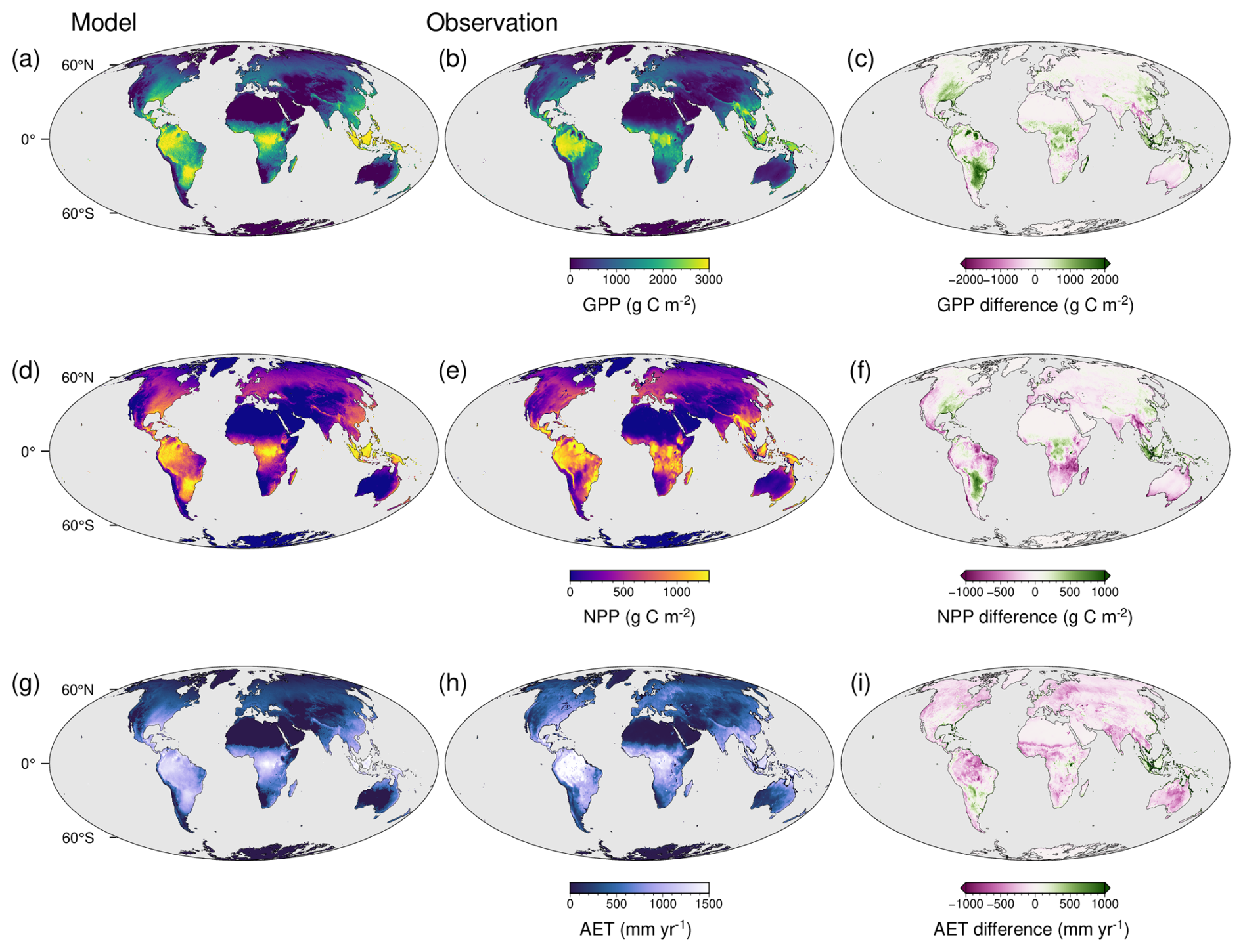
Figure 3 Spatial distribution of model bias in carbon and water fluxes. (a) Modelled gross primary productivity (GPP), (b) MODIS-derived GPP average of the years 2001–2010 (Kern, 2024), and (c) their difference. (d) Modelled net primary productivity (NPP), (e) MODIS-derived NPP average of the years 2001–2010 (Kern, 2024), and (f) their difference. (g) Modelled evapotranspiration (AET), (h) evapotranspiration estimate from Miralles et al. (2011) for the year 2010, and (i) their difference. Differences are given as model minus observed data.

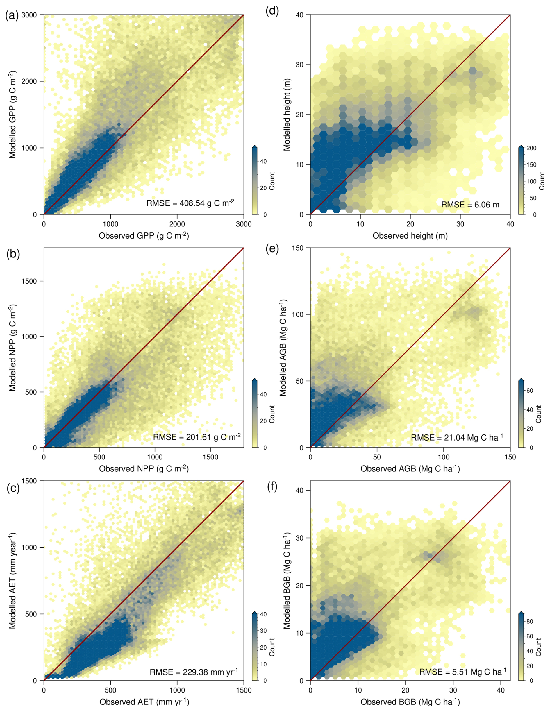
Figure 4 Comparison of modelled and observed carbon and water fluxes (left), and carbon storage (right). (a) Gross primary productivity (GPP), (b), net primary productivity (NPP) and evapotranspiration (AET). (d) Canopy height, (e) above ground biomass carbon (AGB), and (f) below ground biomass carbon (BGB). The 1:1 line is indicated in red. RMSE is the root mean square error. Carbon fluxes from Kern (2024), evapotranspiration from Miralles et al. (2011), height data from Lang et al. (2023), biomass data from Huang et al. (2021) and Santoro et al. (2021).

5.3 Evaluation of modelled vegetation height, biomass, leaf characteristics and phenology

The TREED model allows a reasonable approximation of the first-order distribution of vegetation height and biomass (Figs. 5, 4d–f). For vegetation height, the model generally results in an overly smooth height distribution and tends to overestimate vegetation height compared to the data of the year 2020. The height bias (Fig. 5a–c) needs to be understood in context of the model's underlying structure and bias in NPP predictions. In the model's optimization-based trait allocation (Eq. 49), a surplus NPP will result in a prediction of increased height and biomass growth, until respiratory and tissue turnover carbon investments exceed the surplus carbon from photosynthesis. Through this procedure, the model reproduces the first-order relationship between vegetation height and NPP derived from observational records (Fig. 6a). However, for regions with a positive bias in productivity, such as subtropical South America, the model will overpredict vegetation height. For regions with a small bias or an underprediction of NPP, an overprediction of vegetation height may be caused by an underestimation of carbon turnover processes that reduce the carbon availability for height growth. For example, some environments exhibiting pronounced height overpredictions such as tropical savannahs or the continental interiors of North America may be associated with frequent environmental disturbances, including fires, heat or cold conditions. Such disturbances reduce the longevity of vegetation structures and increase the annual average carbon investments into tissue turnover. A reduced availability of carbon for height growth may also represent carbon investments into trait trade-offs not currently represented, for example a spatially variable partitioning between above-ground and below-ground tissues to optimize water acquisition in seasonally dry environments, or investments for biotic interactions, including defence and competition mechanisms. Finally, in the height comparison it should be noted that the model does not consider present-day human land-use, nor herbivory dynamics. In areas of agricultural production (e.g., cropland and pastures), land use is expected to more strongly affect vegetation structures, such as height and biomass, compared to carbon fluxes like NPP and GPP.

There is a strong relationship between vegetation height and biomass carbon storage, which is reproduced due to the calibration of the allometric constants in the model (Fig. 6b), and which drives the modelled spatial distribution of aboveground and belowground biomass (Fig. 5d–i). Due to the strong biomass to height relationship, mismatches between modelled and observed belowground- and aboveground biomass primarily occur in regions where there is a mismatch in the productivity and height predictions as described above.

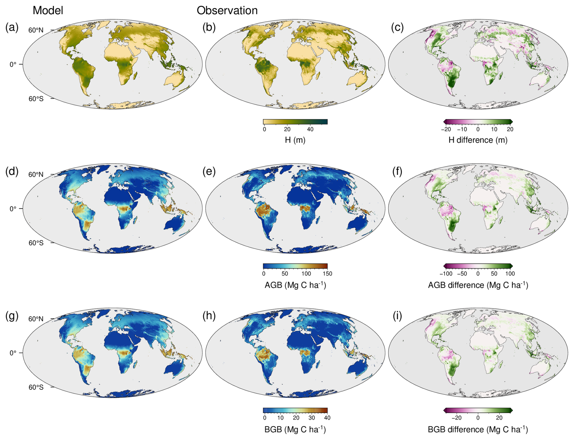
Figure 5 Spatial distribution of model bias in vegetation structure and carbon sequestration. (a) Modelled vegetation height (H), (b) vegetation height estimate for the year 2020 from Lang et al. (2023), and (c) their difference. (d) Modelled above ground biomass density (AGB), (e) above ground biomass estimate from Huang et al. (2021) and Santoro et al. (2021), and (f) their difference. (g) Modelled below ground biomass density (BGB), (h) below ground biomass estimate from Huang et al. (2021) and Santoro et al. (2021), and (i) their difference. Differences are given as model minus observed data.

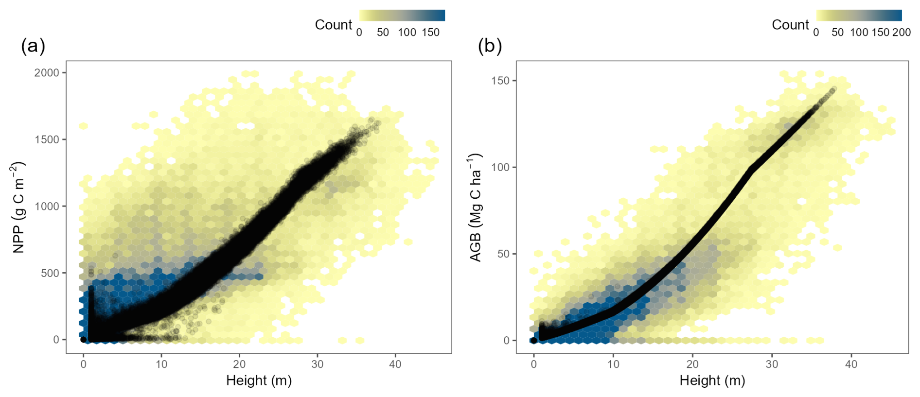
Figure 6 Relationship between vegetation height, carbon fluxes and storage observed in the TREED model and data. (a) Relationship between local rates of net primary productivity (NPP) and vegetation height. The background represents a density plot of observed height from Lang et al. (2023) against NPP data from Kern (2024). The modelled relationship is indicated by black points. The model captures the first-order relationship between height and NPP but does not resolve high NPP/low height combinations, likely related to carbon turnover processes not currently represented in the model. (b) The background represents a density plot of observed height against above ground biomass (AGB) data from Huang et al. (2021) and Santoro et al. (2021). The modelled relationship is indicated by black points. The model's height to AGB relationship was derived with the calibration of the allometric constants (Table 1).

The TREED prediction of deciduous vegetation phenology agrees with the present-day distribution of temperate deciduous broad-leaved forests, with highest frequencies of such growth forms in East Asia, Europe and eastern North America (Fig. 7). Together with the tropics, these regions are associated with predicted leaf longevities of around a year or less. Persistent leaves with longevities of longer than two years are primarily observed in arid or cold regions with a limited growing season length. In line with the carbon economics spectrum (Wright et al., 2004), this tendency indicates a more conservative leaf strategy with lower annual leaf building costs and light acquisition potential but longer persistence. The model captures the major latitudinal patterns of leaf longevity and leaf mass per area (LMA = $\mathrm{1}/$SLA) on the globe, with increasing LMA and leaf longevities for evergreen plants, and a decreasing latitudinal trend observed for deciduous plants (Kikuzawa et al., 2013; Reich et al., 2014; Wang et al., 2023). Latitudinal variations are driven by the availability of light, colder temperatures towards the poles and therefore, decreasing growing season lengths. Deciduous and evergreen plants follow contrasting strategies to adjust to these environmental changes (Wang et al., 2023), which are captured by the model and its optimality-based trait prediction. For deciduous plants, shorter growing season are associated with reduced leaf longevities. To compensate a reduction in the carbon sequestration potential due to the shortened growing season length, deciduous plants require more acquisitive leaf structures and a reduced LMA. Evergreen plants, on the other hand, compensate the shorter growing seasons, reduced light, and colder temperatures by reducing annual carbon investments into leaves, increased LMA, and longer persistence.

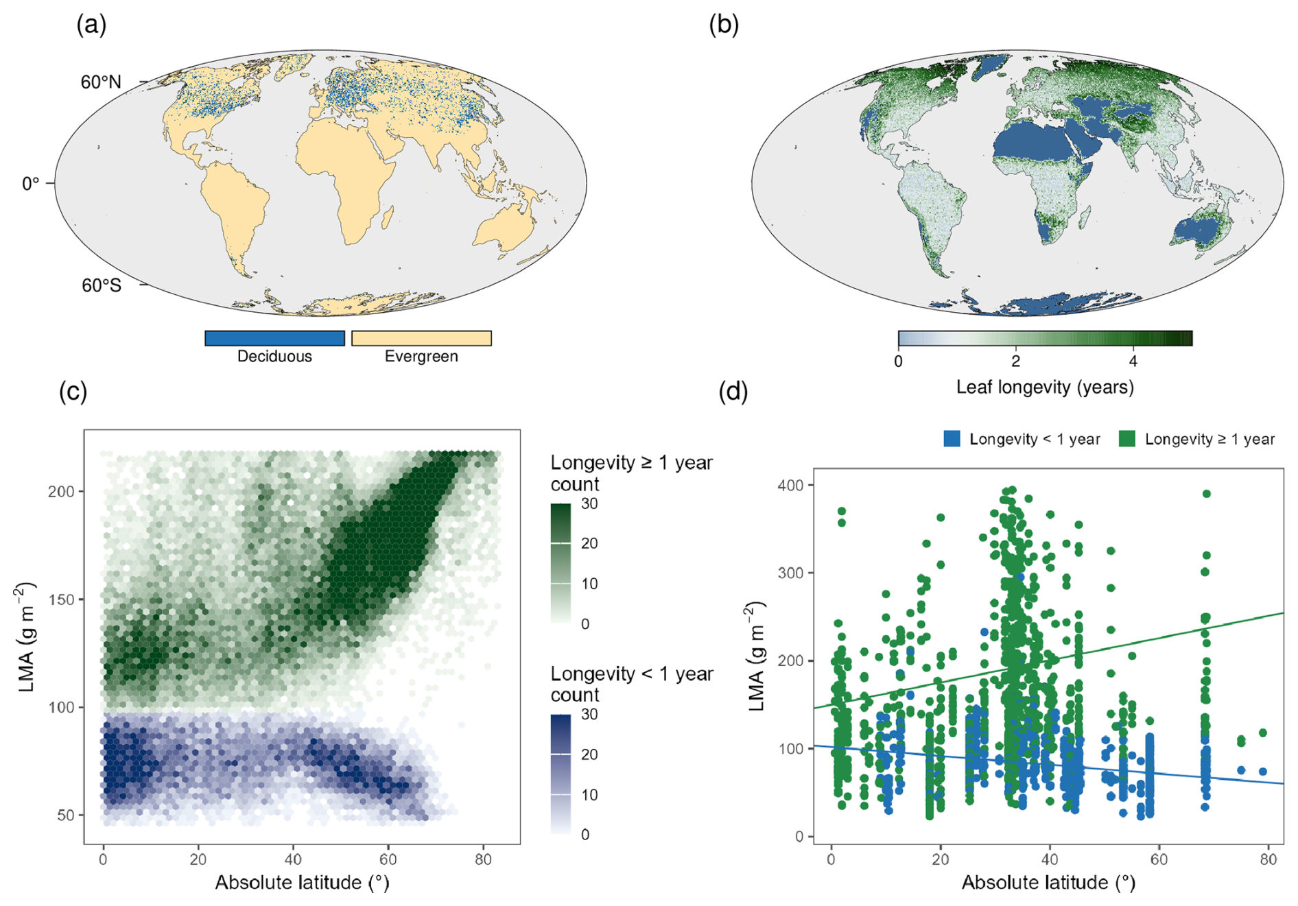
Figure 7 Modelled vegetation phenology and leaf characteristics. (a) Modelled distribution of deciduous and evergreen vegetation. (b) Modelled average leaf lifespan. (c) Modelled latitudinal distribution of leaf longevity and leaf mass per area (LMA). (d) Observed latitudinal distribution of LMA for evergreen (longevity ≥ 1 year) and plants having leaf life cycle durations of less than a year (longevity < 1 year). LMA data from the Glopnet data set (Wang et al., 2023; Wright et al., 2004).

5.4 Evaluation of modelled plant diversity potential

The diversity calculations in TREED capture a large degree of the observed global plant species diversity distribution (Fig. 8), with an underprediction of the species richness in hotspot regions. The diversity potential (DP) in TREED is a compound product of three indices: a functional richness index (FDI), a landscape heterogeneity index (LHI) and a landscape fragmentation index (LFI) (see Eq. 63). The functional diversity index (Fig. 8a) strongly resembles the global pattern of vegetation height and carbon assimilation, indicating that it is primarily a function of the resource availability. In the model, locations with high levels of radiation and water, together with suitable temperatures for photosynthesis, result in a larger range of growth forms and trait combinations that can be sustained and potentially co-exist. The two indices of landscape complexity (LHI and LFI) capture regions of high topographic complexity, including the Andes, Himalayas, the east African mountains and the Alps. Topographic complexity in these regions results in a high variability of climatic conditions and thus vegetation habitats. Further, in topographically complex regions the arrangement of vegetation habitats shows a higher degree of fragmentation, which may be associated with dispersal barriers that promote allopatric speciation processes (i.e., speciation by isolation). Combining functional diversity as an indicator of the local diversity potential and the two landscape metrices effectively captures major biodiversity gradients on Earth, with a spearman ranked correlation between the modelled DP and observed species richness of 0.81. A major underestimation of the diversity potential is observed in South-East Asia, likely driven by an underestimation of the productivity potential in the region (Fig. 3a–f) and thus a reduced functional diversity potential. Similarly, an overprediction of diversity is observed in the central African tropics, likely related to an overprediction of the productivity and functional diversity potential in the region.

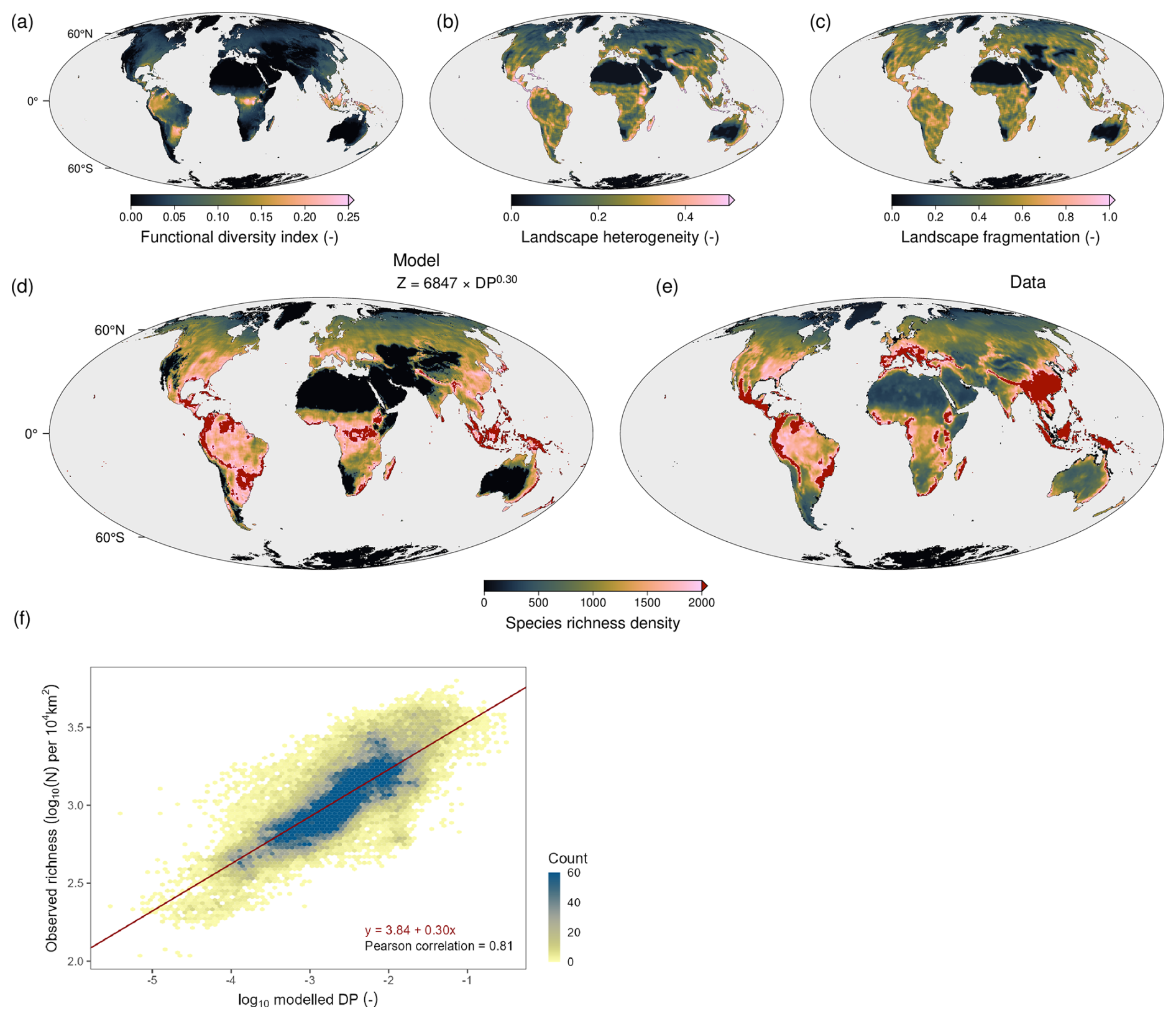
Figure 8 Comparison of modelled plant biodiversity potential and observed species richness data. (a) TREED functional diversity index (FDI), (b) landscape heterogeneity index (LHI), (c) landscape fragmentation index (LFI). Together (a)–(c) represent the components of the diversity potential index ($\mathrm{DP}=\mathrm{FDI}\cdot \mathrm{LHI}\cdot \mathrm{LFI})$. (d) Predicted species richness using a power law fit between observed species richness and the calculated diversity potential index. (e) Observed plant species richness from Cai et al. (2023). Species richness in (d) and (e) is given as number of species per 10 000 km². (f) log-log relationship between modelled diversity potential and observed richness.

6 Paleo-application and eco-evolutionary mode

With regards to computational demand, necessary climatic inputs and model complexity, the TREED model is designed to study vegetation, climate and carbon cycle dynamics over geologic time. The model can either be used to obtain a continuous steady-state prediction of vegetation functioning, structure and diversity, or to study eco-evolutionary transitions of vegetation during periods of environmental change. To illustrate the latter functionality, we apply the model to the Paleocene-Eocene Thermal Maximum (PETM). The PETM was a 5–6 °C global warming event that was triggered by a geologically abrupt release of several thousand Pg of carbon into Earth's atmosphere and oceans (Harper et al., 2024). The climatic perturbation resulted in major shifts in the vegetation distribution and carbon sequestration potential (Bowen, 2013; Bowen and Zachos, 2010; Korasidis et al., 2022). A loss and a 70–100 kyr lagged regrowth of biospheric carbon stocks was suggested to have been an important driver for the long duration and timing the termination of the PETM warming event (Bowen, 2013; Bowen and Zachos, 2010). A perturbation and loss of vegetation-mediated carbon and climate regulation has also been suggested to have driven the severity and duration of other hyperthermal events in Earth's past (Payne et al., 2004; Rogger et al., 2024; Xu et al., 2022, 2025). The TREED model can be used to study global carbon cycle dynamics during such hyperthermal events. Thereby, the model not only produces different carbon sequestration trajectories, but it also tracks the spatial distribution of vegetation traits through time. The trait and carbon flux outputs of TREED can be used in combination with paleobotanical and geochemical records to better understand and constrain the response capacity of vegetation systems to large-scale carbon cycle perturbations in Earth's past (Rogger et al., 2025).

In the following, we force the TREED model with PETM climate model simulation data from Korasidis et al. (2022) and Kiehl and Shields (2013) to approximate the changes in vegetation-mediated carbon cycling across the climatic perturbation. For five time steps, the TREED model is forced with pre-PETM climatic conditions at an atmospheric CO₂ level of 680 ppm, followed by a step change to 1590 ppm which is maintained for another 15 model time steps. We keep the notion of “time steps” rather than actual time units in the following, to emphasize that such numerical experiments could be applied to any model duration from centuries to millions of years with the rates of evolution and dispersal being adjusted by the user accordingly.

In Fig. 9a–d, we show the steady state vegetation height and primary productivity for pre-PETM and peak-PETM CO₂ concentrations. Comparing the two climate states, the model suggests a decreased productivity and vegetation height in tropical and subtropical areas, driven by extreme heat conditions and reduced water availability. In mid to high latitudes, there is a strong increase in vegetation height and productivity, driven by a CO₂ fertilization effect, a higher water-use efficiency and temperatures closer to the optimum photosynthetic temperature between 25 and 30 °C (see Eqs. 18–20). Despite the reduced productivity potential in some tropical and subtropical regions, the total global productivity potential increases from around 85 to around 100 Pg C NPP yr⁻¹.

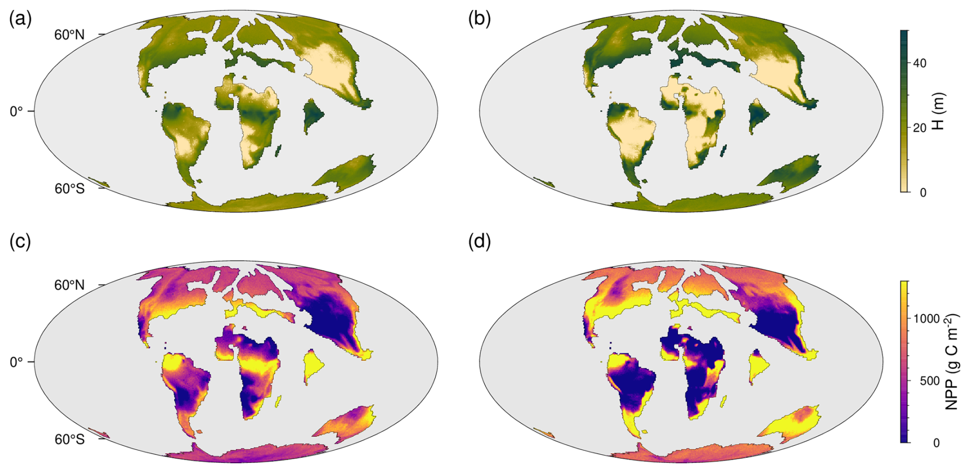
Figure 9 TREED simulation of the PETM. (a) Pre-PETM vegetation height and (c) net primary productivity (NPP) at an atmospheric CO₂ of 680 ppm. (b) PETM vegetation height and (d) NPP at a peak-PETM CO₂ concentration of 1590 ppm.

Whether and how fast the vegetation can capitalize on the globally more optimal productivity conditions strongly depends on the speed of eco-evolutionary adaptation processes and the susceptibility to temperature changes across the transition (Fig. 10). We test a large range of different adaptation scenarios and show that the potential of carbon sequestration across a PETM-like climate transitions strongly depends on the biological capacity to adapt to the environmental changes. The observed range of carbon sequestration trajectories can be categorized in three potential outcomes illustrated in Fig. 10a. In a scenario where the evolutionary rate of functional and climatic trait adaptation is low (e.g., α=0.01), we observe a strong reduction in the productivity potential due to a loss of adaptation of vegetation to the abruptly changing environmental conditions. Only with time, due to continuous dispersal (e.g., dispersal window radius = 600 km) and slow adaptive evolution, the global productivity potential recovers to levels as during pre-PETM conditions. Due to a low evolutionary adaptation potential, no capitalization of the theoretically possible increase in vegetation productivity is observed until the end of the simulation. Under a scenario of fast trait evolution (e.g., α=0.75), only a limited adaptation and productivity lag following the climatic transition is observed. Due to an efficient adaptation of functional and climatic traits, the vegetation can rapidly capitalize on the climatic conditions in favour of increased primary productivity. A reduced dispersal capacity (e.g., dispersal window radius = 200 km) does not strongly affect or offset the comparably fast increase in the global productivity potential. If both evolution and dispersal capacity are kept at an intermediate level (e.g., α=0.1, dispersal window radius = 400 km), an intermediate productivity trajectory is observed. This includes a stress period with a strong reduction of the productivity potential, followed by a recovery and increase of productivity to above pre-PETM levels.

Considering the traits currently included in the TREED model, the capacity of vegetation to endure temperature regimes outside of the original habitat and the capacity to adapt thermal tolerances is found to be the strongest limitation of the global productivity potential (Fig. 10b). When considering no limitation of productivity due to temperature deviations between the local environment and the climatic environment from which the occupying vegetation originates (k_nichebreadth=0), but considering a low evolutionary rate for other functional traits (a_ll,C_leaf, and derived H), we do not observe a drop in vegetation productivity. This is because there is no direct stress effect of temperature on productivity, and further, because if plants are not bound to certain climatic environments, there is an unlimited dispersal-based trait exchange. This would for example mean that tropical trees and associated vegetation traits could migrate into temperate conditions without experiencing any physiological stress. If we assume that plant dispersal and trait evolution is bound to certain thermal limits (k_nichebreadth>0), which themselves are subject to evolutionary adaptation, we observe a temporary drop in productivity because there exist climatic environments with no suiting vegetation immediately available, and because dispersal-based trait exchange only occurs within climatic boundaries. In the default eco-evolutionary model, we assume that plant and trait exchange are bound to thermal limits. With a niche breadth parameter k_nichebreadth of 0.02, the default model assumes that plants can be productive in environments with deviation in the annual average temperature, the coldest month average temperature, and the warmest month average temperature from their original habitat of up to 15 °C. This approximates to the range temperature variability observed within present-day biomes (i.e., observed bioclimatic zones of similar vegetation types and characteristics on the globe). Thereby we assume that there exist plant physiological traits, ecosystem characteristics (e.g., competition, herbivory, pests, etc.) or abiotic conditions (e.g., soils and nutrient availability) which limit vegetation exchange to within such climatic boundaries. With every grid cell of the model being initialized with a climatically optimally adapted vegetation, thermal tolerances start to play a role for productivity if the speed of climatic shifts exceed the dispersal capacity of vegetation (Fig. 10c), and if changes in the temperature distribution exceed the variability observed in the starting climate state. Consequently, we observe a threshold behaviour in the productivity response if we run the model for different land surface warming scenarios across the PETM (Fig. 10d). The climate inputs for modelling the different warming scenarios were derived by linearly interpolating the available climate fields at 680 and 1590 ppm CO₂ to atmospheric CO₂ concentrations corresponding to approximately 2, 4, 6, and 8° of land surface warming (907, 1135, 1362 and 1590 ppm CO₂, respectively). For a land surface warming below 4 °C and under consideration of limited temperature tolerances (k_nichebreadth=0.02), no productivity loss is observed. In these scenarios, there is an effective dispersal-based vegetation redistribution, and climatic conditions allow for an increased global productivity. For land surface warming scenarios of 6 °C or more, a drop and lagged productivity recovery is observed because the speed of climatic change starts to exceed the dispersal-based trait redistribution, and because climatic extremes start to exceed those previously observed. While continuous dispersal-based trait redistribution acts to close the adaptive gap, vegetation is limited by the capacity of adjusting thermal tolerances through acclimation or evolutionary adaptation.

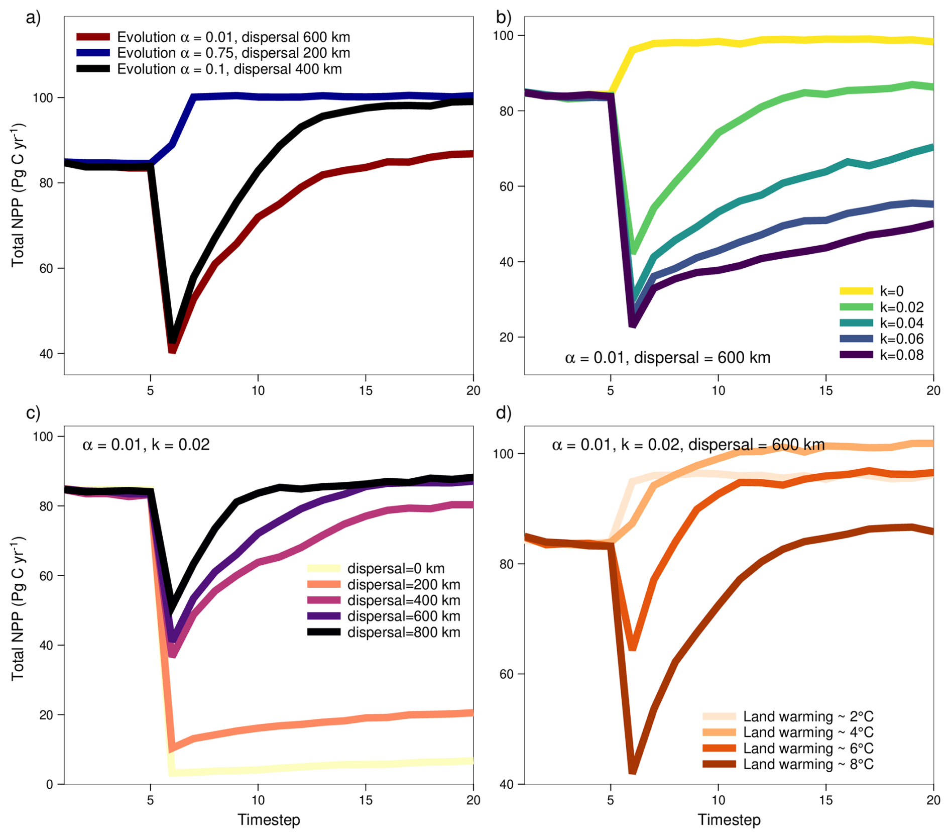
Figure 10 Simulated net primary productivity (NPP) trajectories across the PETM. Simulated NPP trajectories assuming (a) different trait evolution (α) and dispersal rates, (b) different climate niche breadths (k) and thermal tolerances, (c) different dispersal rates, and (d) different land surface warming scenarios.

The model allows to evaluate the spatial dynamics of the vegetation response and eco-evolutionary adaptation dynamics. With the increase in atmospheric CO₂ from 680 to 1590 ppm, there is a strong latitudinal gradient in warming, with highest rates of warming in the high latitudes and dry, continental interiors (Fig. 11a). In low latitudes, productivity gets increasingly limited by drought and heat conditions. In widespread tropical and subtropical regions there is a reduction in precipitation, limiting photosynthesis and carbon sequestration, despite a higher atmospheric CO₂ (Fig. 11b). Additionally, in several low latitude regions, annual average temperatures are modelled to exceed critical thresholds for photosynthesis (Fig. 11c; Eqs. 18–20). In Fig. 11d, we illustrate the heat stress due to a limited eco-evolutionary adaptation response of upper thermal tolerances five time steps after the perturbation, assuming an intermediate adaptation scenario (i.e., α=0.1, dispersal window radius = 400 km). In low latitudes, a reduced productivity potential due to a limited eco-evolutionary adaptation overlaps with regions where productivity is already abiotically limited by reduced precipitation and more abundant heat. These stress conditions reduce the productivity potential in these regions and prevent a fast reoccupation and vegetation recovery. Eco-evolutionary adaptation lags are further widespread in the high latitudes, coinciding with regions with a particularly pronounced warming. The larger warming magnitude increases both the adaptation lag that needs to be closed through evolutionary trait adaptation and prolongs a dispersal-driven trait redistribution due to a widespread productivity loss, with no trait redistribution occurring in unproductive locations. Due to this effect, a further lag may occur in land areas isolated by ocean or unproductive land from which no trait redistribution occurs.

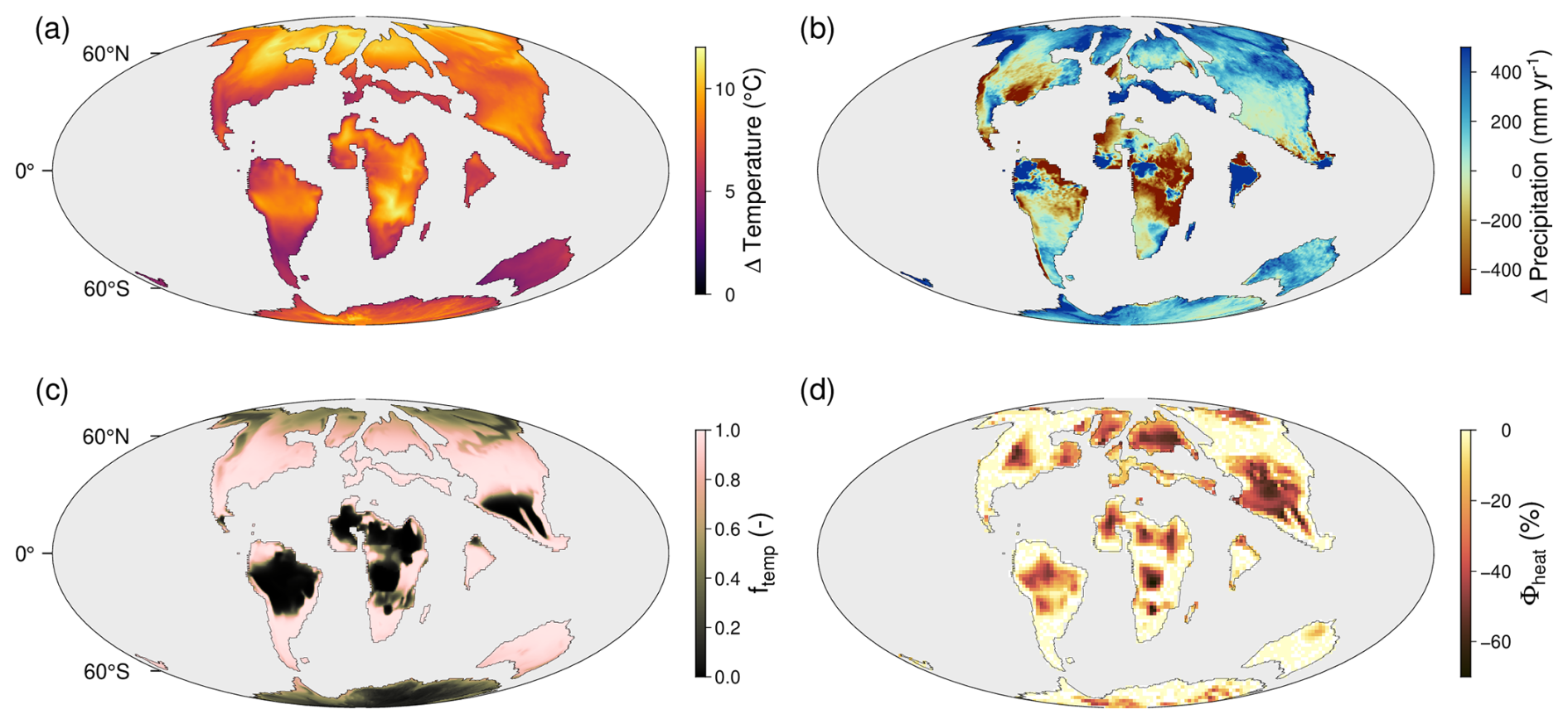
Figure 11 Spatial patterns of vegetation productivity limitation across a Paleocene-Eocene Thermal Maximum warming scenario. (a) Spatial patterns in annual average surface temperature warming for a CO₂ increase from 680 to 1590 ppm. (b) Spatial patterns in annual precipitation changes. (c) Temperature limitation of photosynthesis. Dark areas represent areas where the annual average temperature exceeds critical limits for photosynthesis as defined in the TREED model (> 45 °C). (d) Percentual productivity loss due to an eco-evolutionary adaptation lag of the upper thermal tolerance limit, resulting in a heat stress (Φ_heat), following Eq. (52). The presented heat stress was derived from a simulation conducted at 2° longitude and latitude resolution.

7 Discussion

Using a generalized plant physiology and optimality principles, the TREED model approximates the functioning and structure of present-day vegetation systems, including carbon and water fluxes, height, biomass carbon storage, leaf characteristics, phenology as well as the global distribution of plant species diversity. The model treats trait evolution as an optimization problem under consideration of carbon allocation trade-offs in a continuous trait space, thereby avoiding the use of discrete, pre-parametrized vegetation classes. Our results support the use of organizing principles of biological systems, such as natural selection, to obtain more self-consistent and parameter-scarce mechanistic models of vegetation dynamics under variable climatic conditions, offering new ways to explore the interactions between vegetation dynamics and climatic variation across timescales from the deep past to the present.

7.1 Evaluation of modelled carbon dynamics and traits

Plant carbon and water exchange, as well as biomass carbon storage, represent major forcings in Earth's carbon and climate system. The TREED model can serve as a computationally efficient, first-order approximation of the large-scale patterns of carbon assimilation and sequestration at present and under different planetary climate states in the past and future. Thereby, the model is computationally efficient and uses comparatively little input data of monthly average temperature, radiation, precipitation and cloud cover. This represents an advantage for the main purpose of the model of studying paleoclimate and vegetation dynamics across large timescales, and for conducting sensitivity studies. However, the coarse time stepping likely introduces biases in regions of high climate variability. Global trends in carbon and water fluxes (i.e., GPP, NPP, AET) are predicted with more confidence than vegetation biomass carbon sequestration, indicating that the implemented optimization procedure is better suited to capture the carbon assimilation potential but does not resolve the full variability of how the assimilated carbon is invested into growth and biomass. A discrepancy in the performance of models to predict productivity compared to biomass storage is a feature observed across many vegetation models and is partly explained by the difficulty to resolve carbon turnover times of biomass (Pugh et al., 2020). In the TREED model, the largest biomass carbon pools (heartwood, sapwood, coarse root) are associated with fixed turnover times in the range observed and modelled for the present day (Pugh et al., 2020), while functional relationships determine fine root and leave carbon turnover. In natural systems, turnover of large structural carbon pools is primarily a result of vegetation mortality, driven by a combination of biotic (e.g., competition, herbivory, diseases) and abiotic (e.g., fires, droughts, windthrow) factors (Franklin et al., 1987). A large range of mechanistic formulations exist to approximate these processes, but are associated with considerable uncertainty and differences among models (Pugh et al., 2020). Following other vegetation models (Schaphoff et al., 2018; Sitch et al., 2003), the TREED model further simplifies growth respiration and reproduction carbon costs as fixed fractions of GPP and NPP, respectively. The current implementation of the vegetation carbon turnover and mass balance represents a simple first approximation, with the model being flexible to further develop and test increased complexity formulations of carbon turnover that may depend on environmental conditions or functional trait trade-offs.

In the current TREED version, the considered carbon economic trade-offs and main axes of trait variation include carbon investment into height growth, the leaf carbon pool, leaf longevity and phenology (e.g., Figs. 6 and 7). The underlying allocation dynamics and trade-offs of height growth and leaf carbon economics are well established in both present day vegetation systems (Falster and Westoby, 2003; Valentine and Mäkelä, 2012; Wang et al., 2023; Wright et al., 2004), as well as in the geologic past (McElwain et al., 2024; Soh et al., 2017). With these trade-offs, the model resolves the two main axes of variation in vegetation growth forms observed in plants today (Díaz et al., 2016). However, while capturing mean trends in the form of a single, community-representative average plant per location, the model does not resolve the full range of trait variability and complexity we observe in natural vegetation systems. An increase in the modelled trait variability or the range of independent axes of trait variation would require the formulation of additional trait trade-offs that capture the cost and benefits of growth strategies in given abiotic and biotic environmental conditions. Thereby, the trait trade-off should not be specific to a species or location, but generally applicable across plant species, space and time. The increasing availability of plant functional trait data from various environments at present (Bruelheide et al., 2018; Díaz et al., 2016; Kattge et al., 2020), as well as the geologic past (McElwain et al., 2024), is essential to establish such general trait relationships. The capacity of the TREED model to resolve major patterns in present-day vegetation structure and functioning based on a small number of functional trade-offs illustrates the potential of trait-based models in leading to more generalizable and self-consistent representations of vegetation systems, and may allow a reduction of uncertainty in model-predicted carbon and climate dynamics associated with vegetation parametrizations under environmental conditions of the future (Berzaghi et al., 2020; Fisher et al., 2014) or the deep past (Matthaeus et al., 2023).

7.2 Paleo applications and eco-evolutionary dynamics

Focusing on basic principles of trait functional relationships, a continuous trait space and no pre-parametrized vegetation classes, the TREED model is intended to provide a tool to understand how Earth's climate, topography and vegetation have co-evolved through time. While the fundamental trade-offs of height growth and the leaf economics spectrum that drive the model are expected to also have played out in the distant geologic past (Butrim et al., 2024; Falster and Westoby, 2003; McElwain et al., 2024; Soh et al., 2017), two limitations for the application to the geologic past should be noted. Even though applying a generalized physiology across all plants, the TREED model still takes a present day-derived perspective on traits and whole-plant architecture in the form of the applied allometric and functional relationships. Further, the model assumes a constant theoretically possible trait space for the main varying traits and their combinations. The model does not resolve how the availability of genetic variance may have limited the range of plausible trait combinations through time. The major advantage of TREED with regards to these uncertainties, however, is its capacity to track combined carbon fluxes as well as associated vegetation structures. The model results can thus be compared to combined geochemical records informing about vegetation productivity (Bowen, 2013; Denis et al., 2021), as well as trait structures derived from paleobotanical records (McElwain et al., 2024; Rogger et al., 2025), to assess the validity of currently implemented and future additions of functional trade-offs and allometric relationships.

To study co-evolutionary transitions between the physical environment and vegetation systems, TREED includes eco-evolutionary adaptation processes not currently considered in standard vegetation models, including the capacity of vegetation to adapt to environmental changes through trait evolution and dispersal dynamics (Berzaghi et al., 2020). A limited capacity of vegetation systems to respond to abrupt climatic changes and a loss of vegetation-mediated climate regulation are considered to have strongly shaped global carbon cycle dynamics in the geologic past, and particularly, during episodes of abrupt climatic change (Hull, 2015; Payne et al., 2004; Retallack et al., 1999; Rogger et al., 2024; Xu et al., 2022, 2025). An evaluation of the capacity of vegetation to respond to environmental change is of particular importance considering that the speed of current climate warming may have no precedent in the last 400 million years (Foster et al., 2017). However, our understanding of the plant-climate adaptation process through acclimatization and evolutionary adaptation, the speed, and its limits, remain an active area of research (Bennett et al., 2021; Jezkova and Wiens, 2016; Liu et al., 2020; Schneider et al., 2025; Stemkovski et al., 2025). By combining trait-enabled model predictions, geochemical and palaeobotanical records from Earth's past, the TREED model was developed to help constrain and test hypotheses about the vegetation response to past climatic changes, the speed and capacity of adaptation, and how adaptation may depend on the starting climate state, atmospheric CO₂, or the rate and spatial distribution of climate warming. Obtaining an understanding of these dynamics through geologic time will help to better predict the vegetation responses that may emerge under different scenarios of climate change over the next centuries.

7.3 Plant biodiversity dynamics

We show that the generalized plant physiology and continuous trait space of the TREED model cannot only be used to predict vegetation functioning and structure, but also to estimate locations of a high plant diversity potential. Thereby, we combine measures of local scale diversity (i.e., functional diversity potential) and landscape-scale biodiversity metrics (i.e., landscape heterogeneity and fragmentation of vegetation habitats). The employed metrics are aimed to resolve predominant drivers of plant species richness, including the spatial distribution of productivity-limiting resources such as energy and water, and the distribution of environmental heterogeneity, promoting species diversity though niche differentiation and allopatric speciation (Antonelli et al., 2018; Cai et al., 2023; Kreft and Jetz, 2007; Stein et al., 2014). Our results support that the consideration of these biodiversity drivers captures a large degree of the broad-scale plant species richness distribution on Earth today. As such, in the context of paleoecological research, the model represents a tool to evaluate how topographic and climatic changes throughout Earth's history may have influenced the global distribution of the plant biodiversity either through alteration of the functional diversity potential or landscape dynamics. In the biodiversity estimation, the TREED model takes a purely environment-driven approach by estimating a diversity index based on the current timestep's abiotic environmental conditions. Individual species and their life histories are not resolved. As the biological processes and species life histories that ultimately lead to the realized global biodiversity distribution of a period are not resolved (e.g., speciation, movement, extinction), the predicted biodiversity indices should be considered indicators of an abiotic diversity potential rather than realized diversity.

7.4 Main limitations and future developments

The TREED vegetation model balances a mechanistic, trait-based prediction of vegetation functioning and biodiversity with computational efficiency, allowing for modelling experiments and sensitivity tests across large time scales and under various climate states without pre-defining vegetation types. Key limitations that should be considered in the application of the model include the coarse monthly time stepping, which may not capture non-linear variation in climate and productivity at high temporal resolution. Further, the model does not capture complex ecosystem and carbon turnover dynamics, due to its ecosystem representation by a single, community-representative average plant and simple biomass turnover rules. For the biodiversity estimation, the main limitation of the model arises from its purely abiotic diversity perspective, predicting biodiversity given a distribution of topography and climate, but not resolving species' life histories, biotic interactions, or genetically constrained innovation through time. Regarding eco-evolutionary, non-steady state simulations, the model can track vegetation structures and functioning under different adaptation speeds from no evolutionary adaptation to immediate response, allowing model–data comparisons with paleobotanical records. However, the rates of trait evolution are simplified to a user-defined rate, and there is currently no mechanistic description of evolution, driven by interactions of genetics, traits and the environment. The same applies to the implemented climate niche dynamics, which can be derived based on present-day or past species or biome distributions, while not resolving the underlying physiological mechanisms responsible for observed limitations in climatic tolerances.

Future developments of the TREED model will focus on the consideration and testing of additional functional traits and environment-dependent trait trade-offs. In combination with paleobotanical and present-day trait data, this may help to derive the necessary environment-dependent rules of trait evolution, and to resolve environmental limitations and growth forms not currently represented by the model. Targets for development particularly include functional trade-offs concerning carbon investments into hydraulic traits (e.g., maximum stomatal conductance or xylem conductivity), which are important both in determining the response of vegetation systems to environmental conditions as well as in their impact on the coupled global carbon and water cycle (McElwain et al., 2024). Related to water acquisition, the competition for pre-emptying water resources from competitors may be considered in future model versions, complementing the current light competition scheme. In drought-prone environments, a competitive advantage in securing water may favour the relative allocation of carbon into belowground biomass at the expense of height and aboveground biomass growth (Cabal et al., 2020), which is not currently resolved in the model that assumes a constant root to shoot carbon ratio. Further, alternative models concerning carbon turnover costs may be employed. Possible schemes include environment-dependent vegetation mortality, such as increased carbon turnover in heat, drought or wind-prone environments (Pugh et al., 2020), or susceptibility to biotic stresses depending on environment conditions and functional trait characteristics, e.g., increased herbivory pressures in high temperature environments and for low LMA leaf traits (Currano et al., 2008, 2010). Finally, it is aimed to include recently developed, optimality-based and parameter-scarce models of the photosynthetic carbon assimilation and evapotranspiration into TREED (Stocker et al., 2020), which is the physiologic process currently relying on most pre-defined parameter inputs (e.g., Table 1) and which will help to differentiate the influence of short timescale acclimatization processes of the photosynthetic pathway from long-term evolutionary trait evolution in response to climatic change (Schneider et al., 2025).

8 Conclusions

The trait- and optimality-based vegetation model TREED resolves major patterns in present-day vegetation structure, functioning and diversity by resolving optimal trait allocation strategies of leaf characteristics and height growth across environments. The capacity to capture major vegetation characteristics based on a limited set of functional trait trade-offs emphasizes the potential of trait- and optimality-based vegetation models to advance the representation of vegetation systems under changing environmental conditions. By considering trade-offs that apply across species, space and time, optimality-based models may help to reduce uncertainty in vegetation-mediated Earth system process under climatic conditions fundamentally different from the present, as during Earth's past or under future warm climates. Moreover, by combining a continuous functional trait space with landscape-scale variability in vegetation habitats, the TREED model may help to advance our understanding of the coupled evolution of vegetation productivity and diversity through time.

Vegetation plays a fundamental role in Earth's carbon and climate system, mediating fluxes of carbon, water and energy. A loss of vegetation functions due to abrupt environmental perturbations may trigger feedback dynamics not currently resolved in vegetation and Earth system models. The TREED model approximates eco-evolutionary adaptation dynamics including limited trait evolution and dispersal dynamics to investigate the response capacity of vegetation systems. In combination with geochemical and paleobotanical data, the trait-enabled model may help to better understand and constrain the resilience of vegetation-mediated Earth system functions in the geologic past, as well as under future climatic changes.