Ammonia bidirectional flux model tailored for satellite retrieval parameter inversions

Atmospheric ammonia is an important chemical species for air quality and ecosystem health, and has levels that have either increased or remained stagnant in many regions, in contrast to many other pollutants that have been on the decline in recent decades. As bottom-up emissions inventories for ammonia often have large uncertainties, inversions using ammonia retrievals from satellite-borne instruments are an important tool for improving these emissions inventories. Bidirectional flux models for ammonia give a unified model for emission and dry deposition and have recently been incorporated into a number of atmospheric chemistry models. However, there have been relatively few studies using satellite observations in inversions to refine the parameters in bidirectional flux models. A new bidirectional flux model is introduced that is designed specifically for use with inversion systems. This bidirectional flux model reduces the number of redundant parameters, as viewed by the inversions, to yield a model that is both optimized for use with inversion systems and is easy to implement and maintain in atmospheric chemistry models. Inversions using CrIS ammonia retrievals with this bidirectional flux model implemented in the GEM-MACH air quality forecasting model were performed. With parameters set via inversions, significant differences in surface atmospheric ammonia concentrations between the existing unidirectional model and newer bidirectional model were observed in many agricultural regions, varying by as much as 10 ppbv (or between 50 % and 150 %) in these locations. The bidirectional flux model improved the agreement of GEM-MACH with surface observations in the important growing seasons (spring, summer, fall), with biases decreasing between 14 % and 26 % as compared to the unidirectional model and decreased the error standard deviation between 5 % and 20 %, but also degraded this comparison somewhat for the winter.

1 Introduction

Atmospheric ammonia (NH₃) is a concern for both air quality and ecosystems. It is a precursor for fine particulate matter (Tsimpidi et al., 2007; Makar et al., 2009), which has been associated with cardiovascular and respiratory disease (Pope et al., 2002; Burnett et al., 2014). Excess ammonia deposition can lead to eutrophication and soil acidification (Fangmeier et al., 1994; Krupa, 2003). And while nitrogen oxides and sulfur dioxide levels have broadly declined over the last few decades, the amount of atmospheric ammonia has generally been either stagnant or increasing (Warner et al., 2017; Van Damme et al., 2021). Agriculture (fertilizers, livestock) comprises the most significant contribution to global ammonia emissions, followed by natural sources (vegetation, wild animals, oceans) and biomass burning (Sutton et al., 2013).

Bottom-up ammonia emissions inventories typically have large uncertainties and so often benefit by introducing observational information to refine the inventory's estimates. Ammonia's relatively short atmospheric lifetime and the inhomogeneity of its emissions sources result in atmospheric ammonia concentrations with a fairly inhomogeneous spatial distribution. While precipitation-chemistry observation networks have been used in the past to constrain ammonia emissions (Gilliland et al., 2003, 2006; Paulot et al., 2014), the inhomogeneity of the atmospheric distribution of ammonia makes constraining ammonia emissions with surface networks challenging.

In the last decade and a half, retrieval algorithms for atmospheric ammonia from satellite-borne instruments have successfully been used with instruments such as the Infrared Atmospheric Sounding Interferometer (IASI) (Clarisse et al., 2009; Van Damme et al., 2014), the Tropospheric Emission Spectrometer (TES) (Shephard et al., 2011, 2015), the Atmospheric Infrared Sounder (AIRS) (Warner et al., 2016), and the Cross-track Infrared Sounder (CrIS) (Shephard and Cady-Pereira, 2015; Shephard et al., 2020). While ammonia retrievals generally have larger uncertainties than in situ measurements for single observations, their wide spatial coverage and frequent observations offers a powerful tool for constraining ammonia emissions. Ammonia retrievals from satellite-borne instruments have been used in emissions inversion systems that combine the information contained within the retrievals with emissions inventories to produce an updated set of emissions. Studies have included ammonia emissions inversions using the Goddard Earth Observing System chemistry model (GEOS-Chem) with ammonia retrievals from TES (Zhu et al., 2013; Zhang et al., 2018), IASI (Jin et al., 2023), and CrIS (Cao et al., 2020, 2022), inversions of IASI ammonia retrievals using the Community Multiscale Air Quality (CMAQ) Modeling System (Chen et al., 2021), as well as inversions using CrIS ammonia retrievals with the Global Environmental Multiscale – Modelling Air quality and Chemistry (GEM-MACH) (Sitwell et al., 2022), LOTOS-EUROS (Van Der Graaf et al., 2022), and CHIMERE (Ding et al., 2024) atmospheric chemistry models.

Ammonia emissions inventories are often constructed using emission factors that can be highly uncertain (Anderson et al., 2003) and are dependent on land-use, farming practices, soil properties, and meteorological conditions (Hafner et al., 2018; Genedy and Ogejo, 2023). While the ammonia emissions derived from these inventories can readily be used within air quality models, they do not explicitly incorporate the bidirectional nature of the exchange of ammonia between the surface and the atmosphere (Sutton et al., 1998, 2000; Nemitz et al., 2001). Instead of modeling emission and deposition separately, bidirectional models introduce a unified framework by which chemicals are exchanged between the surface and the atmosphere, which can include the re-emission of deposited species. Typically, bidirectional flux models explicitly model the temperature dependence (and often other meteorologically-dependent factors) of the ammonia surface-atmosphere exchange. The model dependence on other factors, such as soil and plant properties, and agricultural practices, often differ greatly between different bidirectional flux models. Bidirectional flux models can improve the temporal profile of ammonia (Cooter et al., 2010; Cao et al., 2022), ammonium (NH${}_{\mathrm{4}}^{+}$) wet deposition (Pleim et al., 2019), and the agreement with in situ (Wichink Kruit et al., 2012; Pleim et al., 2019) and satellite (Whaley et al., 2018) ammonia observations.

Bidirectional flux models of ammonia have been incorporated into atmospheric chemistry models in recent years, such as CMAQ (Bash et al., 2013; Pleim et al., 2019), GEOS-Chem (Zhu et al., 2015a), GEM-MACH (Whaley et al., 2018; Davis et al., 2025), and LOTOS-EUROS (Wichink Kruit et al., 2012). However, at present, few studies have been conducted examining the ability of satellite ammonia retrievals to improve bidirectional flux models. In Cao et al. (2022), inversions were performed over Europe using CrIS ammonia retrievals with GEOS-Chem with both unidirectional and bidirectional flux schemes. Using a 4DVar inversion method with GEOS-Chem and its adjoint model, Cao et al. (2022) jointly optimized non-fertilizer ammonia emissions and the fertilizer application rate (while an adjoint for soil pH does exist in GEOS-Chem (Zhu et al., 2015a), soil pH was not optimized in this study).

While many bidirectional flux schemes explicitly model the many different factors that govern the surface-atmospheric exchange of ammonia, such as agricultural practices and soil properties, many of the model parameters describing these factors have large uncertainties, as is the case with the emission factors for ammonia. And although ammonia retrievals from satellite-borne instruments can provide valuable information about this exchange, they are unlikely able to provide enough information to constrain all the parameters of a highly detailed bidirectional flux model.

In this work, we introduce a new ammonia bidirectional flux model specifically designed for optimization via inversion methods using satellite retrievals. The goal of this bidirectional flux model will be to adequately describe the ammonia surface-atmospheric exchange in the GEM-MACH model, while reducing the number of parameters that cannot be differentiated by the satellite retrievals. Inversions that optimize model parameters that are highly degenerate with one another (i.e. when different sets of parameter values yield the same model output) can have slower converge rates that may decrease the quality of its results. Accordingly, our bidirectional flux model seeks to minimize the degree of degeneracy/redundancy between model parameters. This has the added benefit of yielding a simpler bidirectional flux model that may be easier to implement and maintain within larger atmospheric chemistry models. The bidirectional flux model parameters are optimized using CrIS ammonia retrievals over North America using the ensemble-variational inversion system described in Sitwell et al. (2022) and the ability of these retrievals to constrain ammonia emission potentials and ground pH will be examined.

2 The GEM-MACH Air Quality Model

This work focuses on developing a new ammonia bidirectional flux model for the GEM-MACH air quality model (Moran et al., 2010; Gong et al., 2015; Pavlovic et al., 2016) that is designed with a parametrization that can easily be tuned with inversion methods using satellite-borne ammonia observations. GEM-MACH is Environment and Climate Change Canada's (ECCC) operational air-quality forecasting system that is built on top of ECCC's operational Global Environmental Multiscale (GEM) weather forecasting model (Côté et al., 1998a, b; Girard et al., 2014). GEM-MACH adds atmospheric gas-phase, aqueous-phase, and heterogeneous chemistry to the GEM model, along with emission and deposition of chemical species.

Our bidirectional flux model was incorporated into version 3.1.0 of GEM-MACH. This version of GEM-MACH has 85 vertical levels that extend from the surface to 0.1 hPa and can be run with both global and limited area horizontal grids. This work uses the operational regional limited area horizontal grid that covers Canada, the United States, and northern Mexico with a grid spacing of 0.09° on a rotated lat/lon grid (corresponding to an average horizontal grid spacing of around 10 km).

GEM-MACH is run sequentially with a refresh of the meteorology every 12 h using the analyses from ECCC's Global Deterministic Prediction System (Buehner et al., 2015). Meteorological/physics variables are integrated using a time step of 5 min, whereas the chemistry variables use a time step of 15 min, and model output is saved every 15 min.

The gas-phase dry deposition in GEM-MACH is based on the resistance models of Wesely (1989) and Zhang et al. (2002) (with some modifications). In this resistance model, gaseous species can be deposited to the surface though deposition to the ground/soil/water or to plant stomata/cuticles/other exposed plant surfaces. Particle dry deposition is implemented in GEM-MACH using the model of Zhang et al. (2001) and wet deposition is calculated using the scheme of Gong et al. (2006).

3 Unidirectional Flux Model

In unidirectional flux models, emission and deposition are modeled separately. In the operational setup for GEM-MACH, (unidirectional) emissions are derived from monthly or annual emissions inventories that are translated into hourly, gridded, speciated emissions files using the Sparse Matrix Operator Kernel Emissions (SMOKE; https://www.cmascenter.org/smoke, last access: 1 July 2024) processing system.

The bottom-up emissions inventories for ammonia are dominated by agricultural sources (fertilizers and livestock). The bidirectional flux model introduced in subsequent sections will act as an alternative model for these agricultural sources. As previously mentioned, the aim of this work is to use ammonia retrievals from satellite-borne instruments to constrain the bidirectional flux model parameters. As ammonia emitted from forest fires may be misattributed to agricultural sources, the bidirectional flux and inversion model will be evaluated for the year 2016 due in part to the relatively low number of forest fires during this year (Munoz-Alpizar et al., 2017; Earl and Simmonds, 2018).

The emissions inventory (used prior to the inversions) used in this work is from version 3.1.2 of the operational GEM-MACH emissions data set. This set of emissions was generated using a 2013 emissions inventory for Canada (https://www.canada.ca/en/environment-climate-change/services/pollutants/air-emissions-inventory-overview.html, last access: 14 March 2025), a 2011-based projected 2017 inventory (version 6.3) for the United States (https://www.epa.gov/air-emissions-modeling/2011-version-63-platform, last access: 24 February 2025) from the US Environmental Protection Agency (EPA), and a 2008 inventory (version 6.2) for Mexico (https://www.epa.gov/air-emissions-modeling/2011-version-62-platform, last access: 24 February 2025) from the US EPA. The emissions inventories from the EPA were derived using a traditional emission factor-based method instead of the bidirectional flux-based inventories used in later versions of the National Emissions Inventory (NEI).

4 General Framework for Bidirectional Flux Modeling

In a bidirectional flux model, both emission and deposition are described using the same model. Dry deposition, the unidirectional flux of gas from the atmosphere to the surface, is commonly modeled with resistance models that are analogous to the resistances in electrical circuits. As these resistance models permit substances to travel in either direction, by adding emission source terms to a deposition model, the resistance model may be used to model the transfer from the surface to the atmosphere as well. In this case, the bidirectional flux model is comprised of (a) a resistance model that connects the atmosphere to the surface and (b) a model of the emission sources. This section describes these two components in a general framework. Our specific bidirectional flux model that makes use of this framework will follow in Sect. 5.

4.1 Resistance Model

The resistance model connects the top of the surface atmospheric layer with concentration χ_a to the surface, as seen in Fig. 1. The total resistance $R_{\mathrm{t}}=R_{\mathrm{a}}+R_{\mathrm{b}}+R_{\mathrm{c}}$ is decomposed into a series of different resistances: The aerodynamic resistance R_a which characterizes transport through the surface layer to the quasi-laminar sublayer, the quasi-laminar resistance R_b that models the transport through the quasi-laminar sublayer, and finally the surface resistance R_c that models the air-surface exchange. The surface resistance is often decomposed into different parallel pathways that characterize different modes of atmospheric-surface transport. For this general model, we consider N_c different surface types, where each surface pathway i is connected to a surface concentration ${\mathit{\chi }}_{\mathrm{s}}^{\left(i\right)}$ associated with a surface resistance $R_{\mathrm{c}}^{\left(i\right)}$.

Figure 1 General resistance model describing atmospheric-surface exchange.

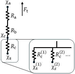
This resistance model can be represented in terms of total equivalent quantities, as represented on the left side of Fig. 1, where the total surface resistance R_c and the equivalent total surface concentration χ_s are expressed in terms of the individual surface pathways as

$$\begin{array}{}\text{(1a)}& {\displaystyle }{R}_{\mathrm{c}}^{-\mathrm{1}}=\sum _{i=\mathrm{1}}^{N_{\mathrm{c}}}(R_{\mathrm{c}}^{\left(i\right)}{)}^{-\mathrm{1}},\text{(1b)}& {\displaystyle }{\mathit{\chi }}_{\mathrm{s}}=\sum _{i=\mathrm{1}}^{N_{\mathrm{c}}}{\displaystyle \frac{R_{\mathrm{c}}}{R_{\mathrm{c}}^{\left(i\right)}}}{\mathit{\chi }}_{\mathrm{s}}^{\left(i\right)}.\end{array}$$

Written in terms of these total quantities, the flux F_t at the top of the surface layer can be expressed as

$$\begin{array}{}\text{(2)}& F_{\mathrm{t}}=v_{\mathrm{d}}({\mathit{\chi }}_{\mathrm{s}}-{\mathit{\chi }}_{\mathrm{a}}),\end{array}$$

where $v_{\mathrm{d}}=\mathrm{1}/R_{\mathrm{t}}$ is the deposition velocity. Details of the derivation of Eqs. (1b) and (2) can be found in Appendix A. When χ_s>χ_a net flux is to the atmosphere and when χ_s<χ_a net flux is to the surface. For unidirectional models where the resistance model is used only for deposition, all surface concentrations ${\mathit{\chi }}_{\mathrm{s}}^{\left(i\right)}$ are set to zero and emissions are supplied separately to the atmospheric chemistry model.

Lastly, it will be convenient to introduce the pathway-weighted deposition velocity $v_{\mathrm{d}}^{\left(i\right)}$ for surface pathway i defined as

$$\begin{array}{}\text{(3)}& v_{\mathrm{d}}^{\left(i\right)}\equiv {\displaystyle \frac{R_{\mathrm{c}}}{R_{\mathrm{c}}^{\left(i\right)}}}{v}_{\mathrm{d}},\end{array}$$

so that we have $v_{\mathrm{d}}={\sum }_{i=\mathrm{1}}^{N_{\mathrm{c}}}{v}_{\mathrm{d}}^{\left(i\right)}$ and the total flux F_t can be expressed as

$$\begin{array}{}\text{(4)}& F_{\mathrm{t}}=\sum _{i=\mathrm{1}}^{N_{\mathrm{c}}}{v}_{\mathrm{d}}^{\left(i\right)}({\mathit{\chi }}_{\mathrm{s}}^{\left(i\right)}-{\mathit{\chi }}_{\mathrm{a}}).\end{array}$$

Note that $v_{\mathrm{d}}^{\left(i\right)}\le v_{\mathrm{d}}$, which reflects that only a portion of the ammonia leaving from the ground may be emitted at top of the surface layer as some ammonia can be (re)absorbed through other surface pathways that act as a sink.

4.2 Exchange of Ammonia Between the Atmosphere and the Surface

Under equilibrium conditions, combining Henry's law with the aqueous dissociation equilibrium between NH₃ and ${\mathrm{NH}}_{\mathrm{4}}^{+}$ relates the gaseous ammonia concentration ${\mathit{\chi }}_{\mathrm{s}}^{\left(i\right)}$ and aqueous ammonium concentration $\left[{\mathrm{NH}}_{\mathrm{4}}^{+}\right(\mathrm{aq}\left)\right]$. This relation (at 1 atm) can be expressed as (Sutton et al., 1994)

$$\begin{array}{}\text{(5)}& {\mathit{\chi }}_{\mathrm{s}}^{\left(i\right)}={\mathrm{\Gamma }}_{\mathrm{s}}^{\left(i\right)}{\displaystyle \frac{A}{T}}{e}^{-B/T},\end{array}$$

where ${\mathrm{\Gamma }}_{\mathrm{s}}\equiv \left[{\mathrm{NH}}_{\mathrm{4}}^{+}\right]/\left[{\mathrm{H}}^{+}\right]$ is known as the emissions potential, the gaseous ammonia concentration at equilibrium is known as the compensation point, and A = 161 500 mol K L⁻¹ and B = 10 380 K are constants (Nemitz et al., 2000). As in the previous section, the superscript (i) labels particular surface pathways.

The relation in Eq. (5) is commonly used to model the exchange of atmospheric ammonia with the ground, which can include exchange between soil pores and soil water, exchange with plant litter, and volatilization from fertilizers (Nemitz et al., 2001; Massad et al., 2010), as well as the exchange between the gaseous ammonia in the sub-stomatal cavities of plants and ammonium in the apoplastic fluid (Nemitz et al., 2000, 2001).

5 Dynamic Ammonium Pool Models

Our aim is to develop a bidirectional flux model with a dynamic ammonium pool with parameters that can be tuned through the inversion process. The bidirectional flux of ammonia was incorporated into CMAQ using information from the Environmental Policy Integrated Climate (EPIC, https://epicapex.tamu.edu/epic/, last access: 13 May 2026) agricultural ecosystem model, interfaced with the Fertilizer Emission Scenario Tool (FEST‐C, https://www.cmascen-ter.org/fest-c/, last access: 13 May 2026), to provide the soil ammonium concentration used in its bidirectional flux model (Pleim et al., 2019). While EPIC contains detailed agricultural information, the amount and complexity of information may not be ideal for systems designed for inversions using satellite retrievals.

In contrast, the bidirectional flux model implemented in GEOS-Chem (Zhu et al., 2015a) uses a simplified model of fertilizer application and nitrification of ammonium in soil to model the bidirectional flux of ammonia from soil. Cao et al. (2022) demonstrated that the fertilizer application rate can be adjusted by inversion algorithms using ammonia satellite retrievals. The bidirectional flux model introduced in this work further simplifies the model of Zhu et al. (2015a) by connecting it to the capacitance model introduced in Sutton et al. (1998).

5.1 Ammonia Source Specification

Our bidirectional flux model for ammonia utilizes the same dry deposition resistance model in GEM-MACH that was described in Sect. 2, but has non-zero values set for the source concentrations ${\mathit{\chi }}_{\mathrm{s}}^{\left(i\right)}$. The details of how the source concentrations ${\mathit{\chi }}_{\mathrm{s}}^{\left(i\right)}$ are specified are described in this section.

The circuit diagram for our bidirectional flux model is shown in Fig. 2. The top portion of the figure shows the standard surface resistances used in GEM-MACH, comprised of deposition pathways to plant stomata, cuticles, other plant surfaces, and the ground, associated with resistance R_st, R_cut, R_oth, and R_g, respectively.

Figure 2 Capacitance-based bidirectional flux model for ammonia.

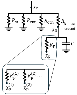
We make the simplifying assumption that only the ground source concentration χ_g has a non-zero value, while the other three surface pathways have their source concentrations set to zero so that they act only as sinks. As mentioned in Sect. 4.2, the bidirectional exchange with stomata can be non-negligible. However, while in non-agricultural settings the stomatal emissions potential can be as large or larger than the ground/soil emissions potential (Zhang et al., 2010), the ground emissions potential for fertilized grounds can exceed these values by many orders of magnitude (Massad et al., 2010). As it is unlikely that our satellite ammonia retrievals contain enough information to differentiate between the stomatal and ground ammonia emissions, and agricultural emissions are the dominant ammonia emissions source within our model domain, we set the stomatal emissions potential to zero to reduce the number of parameters in the bidirectional model. However, this does not necessarily imply that there is no bidirectional ammonia exchange between the atmosphere and the other three pathways, only that we fold all contributions to the bidirectional exchange into the ground pathway for the sake of computational simplicity.

5.2 Capacitance Model of the Ammonium Pool

Sutton et al. (1998) included a model for the bidirectional flux of ammonia from plant stomata based on extending the resistance-based deposition model to include a capacitor that can store and release ammonium. Inspired by this model, we model the ground/soil ammonium pool by a capacitor with capacitance C, as depicted in Fig. 2. The capacitor is placed in parallel with N_p ammonium sources/sinks, where each pathway j is associated with a source concentration ${\mathit{\chi }}_{\mathrm{p}}^{\left(j\right)}$ and a resistance $R_{\mathrm{p}}^{\left(j\right)}$, as illustrated at the bottom of Fig. 2. At this point, we do not specify the specific ammonium sources (with ${\mathit{\chi }}_{\mathrm{p}}^{\left(j\right)}>\mathrm{0}$) or sinks (with ${\mathit{\chi }}_{\mathrm{p}}^{\left(j\right)}=\mathrm{0}$), but sources can include fertilization and livestock and examples of sinks are nitrification in soil and ammonium lost due to runoff or drainage. Instead, we gather these pathways into a single equivalent source/sink with a total resistance R_p and an equivalent concentration χ_p, given by

$$\begin{array}{}\text{(6a)}& {\displaystyle }{R}_{\mathrm{p}}^{-\mathrm{1}}=\sum _{j=\mathrm{1}}^{N_{\mathrm{p}}}(R_{\mathrm{p}}^{\left(j\right)}{)}^{-\mathrm{1}},\text{(6b)}& {\displaystyle }{\mathit{\chi }}_{\mathrm{p}}=\sum _{j=\mathrm{1}}^{N_{\mathrm{p}}}{\displaystyle \frac{R_{\mathrm{p}}}{R_{\mathrm{p}}^{\left(j\right)}}}{\mathit{\chi }}_{\mathrm{p}}^{\left(j\right)}.\end{array}$$

We note that the expressions above for R_p and χ_p have the same form as R_c and χ_s in Eqs. (1a) and (1b).

The ammonium ground surface concentration at the fluid/gas boundary Q_g can be expressed by $Q_{\mathrm{g}}=h\left[{\mathrm{NH}}_{\mathrm{4}}^{+}\right]$, where h is the fluid depth. Using Eq. (5), the capacitance $C=Q_{\mathrm{g}}/{\mathit{\chi }}_{\mathrm{g}}$ of the ground ammonium pool is given by

$$\begin{array}{}\text{(7)}& C=h{\displaystyle \frac{T_{\mathrm{g}}}{A}}{e}^{B/T_{\mathrm{g}}}\left[{\mathrm{H}}^{+}\right],\end{array}$$

where T_g is the ground temperature.

As the flux coming out of the capacitor can be expressed by $-\mathrm{d}{Q}_{\mathrm{g}}/\mathrm{d}t$, Kirchhoff's current law implies

$$\begin{array}{}\text{(8)}& {\displaystyle \frac{\mathrm{d}{Q}_{\mathrm{g}}}{\mathrm{d}t}}={\displaystyle \frac{{\mathit{\chi }}_{\mathrm{c}}-{\mathit{\chi }}_{\mathrm{g}}}{R_{\mathrm{g}}}}+{\displaystyle \frac{{\mathit{\chi }}_{\mathrm{p}}-{\mathit{\chi }}_{\mathrm{g}}}{R_{\mathrm{p}}}}.\end{array}$$

Equation (8) shows that the aqueous ammonium pool evolves with time to establish an equilibrium between the canopy ammonia concentration χ_c and the ammonium source χ_p. To find the time evolution of the ground emissions potential Γ_g, we make the simplifying assumption that the product h[H⁺] is constant in time, so that $\mathrm{d}{Q}_{\mathrm{g}}/\mathrm{d}t=h\left[{\mathrm{H}}^{+}\right]\mathrm{d}{\mathrm{\Gamma }}_{\mathrm{g}}/\mathrm{d}t$. After some algebra, which can be found in Appendix A, Eq. (8) can be written in terms of the ground emissions potential Γ_g as

$$\begin{array}{}\text{(9)}& {\displaystyle \frac{\mathrm{d}{\mathrm{\Gamma }}_{\mathrm{g}}}{\mathrm{d}t}}={\displaystyle \frac{\mathrm{1}}{{\mathit{\tau }}_{\mathrm{a}}}}({\mathrm{\Gamma }}_{\mathrm{a}}-{\mathrm{\Gamma }}_{\mathrm{g}})+{\displaystyle \frac{\mathrm{1}}{{\mathit{\tau }}_{\mathrm{p}}}}({\mathrm{\Gamma }}_{\mathrm{p}}-{\mathrm{\Gamma }}_{\mathrm{g}}),\end{array}$$

where we have defined Γ_a and Γ_p analogously to Γ_s in Eq. (5) as

$$\begin{array}{}\text{(10a)}& {\displaystyle }{\mathrm{\Gamma }}_{\mathrm{a}}\equiv {\mathit{\chi }}_{\mathrm{a}}{\displaystyle \frac{T_{\mathrm{g}}}{A}}{e}^{B/T_{\mathrm{g}}},\text{(10b)}& {\displaystyle }{\mathrm{\Gamma }}_{\mathrm{p}}\equiv {\displaystyle \frac{{\mathit{\chi }}_{\mathrm{p}}}{\mathrm{1}+\mathit{\alpha }}}{\displaystyle \frac{T_{\mathrm{g}}}{A}}{e}^{B/T_{\mathrm{g}}}.\end{array}$$

In the equation above, α is a factor that accounts for the flow into the other surface pathways (i.e. through R_st, R_cut, and R_oth) given by

$$\begin{array}{}\text{(11)}& \mathit{\alpha }\equiv {\displaystyle \frac{R_{\mathrm{p}}}{R_{\mathrm{t}}}}{\displaystyle \frac{R_{\mathrm{c}}}{R_{\mathrm{g}}}}\left(\mathrm{1}-{\displaystyle \frac{R_{\mathrm{c}}}{R_{\mathrm{g}}}}\right)\left({\displaystyle \frac{R_{\mathrm{t}}}{R_{\mathrm{c}}}}-\mathrm{1}\right).\end{array}$$

We have also identified the RC time constants τ_a and τ_p for the atmosphere and ammonium source, respectively, as

$$\begin{array}{}\text{(12a)}& {\displaystyle }{\mathit{\tau }}_{\mathrm{a}}={\displaystyle \frac{R_{\mathrm{g}}}{R_{\mathrm{c}}}}{R}_{\mathrm{t}}C,\text{(12b)}& {\displaystyle }{\mathit{\tau }}_{\mathrm{p}}={\displaystyle \frac{\mathrm{1}}{\mathrm{1}+\mathit{\alpha }}}{R}_{\mathrm{p}}C,\end{array}$$

which are the time scales for the ammonium pool to reach equilibrium with the atmosphere and ammonium sources, respectively. Equation (9) shows that Γ_g evolves in time to establish an equilibrium between the atmospheric ammonia source Γ_a and the aqueous ammonium source Γ_p, which is shown diagrammatically in Fig. 3.

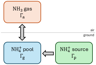
Figure 3 Diagram showing the influence of the atmospheric ammonia potential Γ_a and the aqueous ammonium source Γ_p on the ground emissions potential Γ_g.

With the prognostic equation for the ground emissions potential given by Eq. (9) and χ_g related to Γ_g by Eq. (5), the bidirectional exchange of ammonia between the surface and atmosphere given in Eq. (4) can be computed. These equations reference total parameters such as χ_p and Γ_p, but do not reference parameters for individual pathways (i.e. parameters with the superscript (j)). Therefore, if we can adequately set these total parameters, then it is not necessary to determine the individual source/sink quantities of the ammonium pool. In our case, as the bidirectional flux model parameters will be determined through top-down inversions that use retrievals from satellite-borne instruments that are only sensitive to these total parameters, this yields a bidirectional flux model with minimal parameters that is tailored for use in inversion systems.

In summary, the evolution of the ground emissions potential in our bidirectional flux model is determined by the parameters Γ_p and τ_p, which sets the ammonium source level and response timescale, respectively. Although the intention is to deal with these total parameters directly, we note that Γ_p and τ_p can be expressed in terms of individual pathways as

$$\begin{array}{}\text{(13a)}& {\displaystyle }{\mathrm{\Gamma }}_{\mathrm{p}}={\displaystyle \frac{T_{\mathrm{g}}}{A}}{e}^{B/T_{\mathrm{g}}}{\displaystyle \frac{\sum _{j=\mathrm{1}}^{N_{\mathrm{p}}}{\mathit{\chi }}_{\mathrm{p}}^{\left(j\right)}/R_{\mathrm{p}}^{\left(j\right)}}{\sum _{j=\mathrm{1}}^{N_{\mathrm{p}}}\mathrm{1}/R_{\mathrm{p}}^{\left(j\right)}}},\text{(13b)}& {\displaystyle }{\mathit{\tau }}_{\mathrm{p}}^{-\mathrm{1}}=\sum _{j=\mathrm{1}}^{N_{\mathrm{p}}}({\mathit{\tau }}_{\mathrm{p}}^{\left(j\right)}{)}^{-\mathrm{1}}.\end{array}$$

5.3 Emissions Potential Parametrization

With the prognostic equation for the emissions potential derived from the capacitance model outlined in the previous section, we now set the parameters for the ammonium pool. From Eq. (9), the model parameters that need to be set are Γ_p, τ_p, and τ_a.

Γ_p, which describes the sources of ammonium to the ground, is taken as a spatially-varying 2D field on the same horizontal grid as described in Sect. 2, allowing for a unique field for every month. In this work, Γ_p will represent agricultural sources (both fertilizer and livestock), while separate non-agricultural ammonia emissions that account for ≲1 % of total emissions will be accounted for using the unidirectional emissions model. As ammonia emissions from cattle originate primarily from excreted nitrogen in manure (Lee et al., 2025), we make the same assumption as in Zhu et al. (2015b) in which all ammonia emissions from livestock are assumed to originate from manure. We can then treat both the livestock and fertilizer emissions using the same emissions modeling framework. As such, model parameters that reference the ground or soil should be understood to be inclusive of manure produced by livestock.

The RC constant τ_p is the time scale for the ground emissions potential to equilibriate to Γ_p. Although this time scale can depend on temperature and soil moisture (Stange and Neue, 2009; Vira et al., 2020), we simply set this parameter to a constant value. In their bidirectional flux model, Massad et al. (2010) proposed using a value just under three days for the time constant associated with the dynamics of the ground emissions potential following fertilizer application. Following Massad et al. (2010), we set τ_p to a value of three days.

Using the expression for capacitance in Eq. (7), the time constant τ_a given in Eq. (12a) can be computed by

$$\begin{array}{}\text{(14)}& {\mathit{\tau }}_{\mathrm{a}}={\displaystyle \frac{R_{\mathrm{g}}}{R_{\mathrm{c}}}}{R}_{\mathrm{t}}{d}_{\mathrm{s}}\mathit{\theta }{\displaystyle \frac{T_{\mathrm{g}}}{A}}{e}^{B/T_{\mathrm{g}}}\left[{\mathrm{H}}^{+}\right],\end{array}$$

where we have expressed the fluid depth h in soil pores in terms of the soil depth d_s and the volumetric water content of soil θ as h=d_sθ. The resistances R_g, R_c, and R_t are given by the standard deposition resistance parametrization used in GEM-MACH described in Sect. 4.1, while the soil water content θ and ground/soil temperature T_g are computed using the two-level Interaction Soil-Biosphere-Atmosphere (ISBA) surface model (Noilhan and Mahfouf, 1996) that has been incorporated into GEM-MACH. The soil depth d_s is set to 2 cm, as done in Zhu et al. (2015a) and Vira et al. (2020). Lastly, [H⁺] is parametrized through the ground/soil pH, which was set as a 2D field on GEM-MACH's horizontal grid.

In summary, the free parameters for the bidirectional flux model are the ammonium source term Γ_p that sets the level of ground ammonium and the ground pH which determines the rate at which the ammonium pool reaches equilibrium with ammonia in the atmosphere. Figure 4 shows the values of τ_a as a function of pH and ground temperature (with $R_{\mathrm{t}}{R}_{\mathrm{g}}/R_{\mathrm{c}}=\mathrm{300}$ s m⁻¹ and θ=0.1 chosen to represent typical values). In this figure, we can see that high values of pH and ground temperature result in a low capacitance and short atmosphere/ground equilibrium time scales. In this example, for a pH of 8 and a ground temperature of 25 °C, τ_a is just under three hours, so in this case the ammonium pool will reach equilibrium with atmospheric ammonia relatively quickly. In contrast, for a pH of 6 and a ground temperature of 10 °C, τ_a is over 100 d and so the ground emissions potential will be relatively insensitive to sub-seasonal changes in ammonia levels.

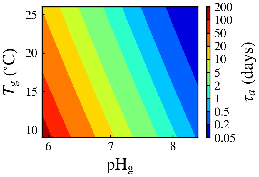
Figure 4 Equilibrium time scale τ_a between atmospheric ammonia and the ground ammonium pool, as computed by Eq. (14), using parameter values of $R_{\mathrm{t}}{R}_{\mathrm{g}}/R_{\mathrm{c}}=\mathrm{300}$ s m⁻¹, θ=0.1, and d_s=2 cm.

If τ_a≫τ_p, then Γ_g≈Γ_p after a few multiples of τ_p in time. As Γ_p was chosen to be a 2D field that is constant within a month, if τ_a is much longer than a month, Γ_g will only evolve to reach equilibrium with Γ_p and not with the atmospheric ammonia. In this limit, the bidirectional flux model is similar to models where the Γ_g values are static. Accordingly, the dynamic nature of the ammonium pool is only evident when τ_a is (roughly) less than or equal to one month.

6 Observations

The bidirectional flux model developed in this work was formulated with the goal of tuning its parameters with inversions using satellite-borne retrievals. This section gives a brief description of the CrIS ammonia retrievals that are used in the inversions, as well as the ammonia surface observations that are used for validation of the inversion results.

6.1 CrIS Ammonia Retrievals

CrIS is a Fourier transform spectrometer that measures the infrared spectrum with a swath width of ∼ 2200 km and a ∼ 14 km spatial resolution at nadir. CrIS instruments are currently aboard the Suomi National Polar-orbiting Partnership (SNPP), NOAA-20, and NOAA-21 satellites. As the year 2016 is used for evaluation, before NOAA-20 and NOAA-21 were launched, all retrievals used in this study come from the instrument aboard the SNPP satellite. SNPP is in a sun-synchronous orbit with local overpass times at approximately 01:30 and 13:30, although only day-time retrievals are used in the inversions.

Ammonia retrievals are made using version 1.6.4 of the CrIS Fast Physical Retrieval (CFPR) algorithm (Shephard and Cady-Pereira, 2015; Shephard et al., 2020; White et al., 2023) that is based on the TES ammonia retrieval algorithm (Shephard et al., 2011), which minimizes the difference between observed radiances and radiances generated by a radiative transfer model (Moncet et al., 2008). This minimization also includes an a priori regularization term, where the a priori profile is chosen as one of three possible profiles that aim to represent ammonia profiles for background, moderate source, and high source regions. Retrievals are made on 14 pressure levels, with the averaging kernel typically peaking in the boundary layer. Version 1.6.4 of the CFPR algorithm also accounts for non-detects where the ammonia signal is below the detection limit of the instrument (White et al., 2023). Only retrievals over land with a minimum degrees of freedom of 0.1 are used in the inversions.

6.2 Surface Observation Networks

Surface observations of ammonia from Canada's National Air Pollution Surveillance (NAPS; https://www.canada.ca/en/environment-climate-change/services/air-pollution/monitoring-networks-data/national-air-pollution-program.html, last access: 25 May 2026) network and the US's Ammonia Monitoring Network (AMoN; http://nadp.slh.wisc.edu/amon, last access: 13 May 2026) are used for validation. AMoN, part of the US National Atmospheric Deposition Program (NADP), uses Radiello^® passive diffusion samplers to measure ammonia levels over two-week periods. The NAPS stations that measure ammonia do so using citric acid-coated denuders that measure ammonia levels over a 24 h period every three or six days. The locations of the 101 AMoN stations and 12 NAPS stations, which account for 3065 and 1080 observations in total, respectively, are displayed in Fig. 5.

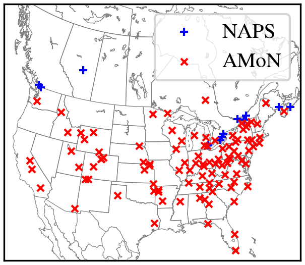
Figure 5 Station locations for the NAPS and AMoN networks with ammonia observations available for 2016.

Validation with the surface observations is done by examining the changes in the bias, standard deviation of errors (STDE), the Pearson correlation coefficient (ρ), and root mean square error (RMSE), the definition of which can be found in Appendix B. When the bias, STDE, or RMSE are expressed as a percentage, the denominator is taken as the annual mean observation value.

7 Flux Model Inversions

The inversions used in this study use the ensemble-variational inversion system described in detail in Sitwell et al. (2022). A summary of this inversion method is provided in Sect. 7.1, followed by the specification of the ensemble used for this study in Sect. 7.2.

7.1 Inversion Procedure

The goal of an inversion is to find an optimal synthesis of observational and a priori (background) model information. For our application, the model state x is comprised of ammonia atmospheric concentrations c and bidirectional flux model parameters and/or other emissions parameters β, which can be written in block form as

$$\begin{array}{}\text{(15)}& \mathit{x}=\left[\begin{array}{c}\mathit{c}\\ \mathit{\beta }\end{array}\right].\end{array}$$

The inversion algorithm seeks a change Δβ, known as the increment, that results in a change Δc to the atmospheric ammonia concentrations that improves the agreement with the observations y. In a variational algorithm, the inversion is performed by minimizing a cost function J, which for our case is given by

$$\begin{array}{}\text{(16)}& \begin{array}{rl}J& ={\displaystyle \frac{\mathrm{1}}{\mathrm{2}}}\mathrm{\Delta }{\mathit{\beta }}^{\mathrm{T}}{\mathbf{B}}_{\mathit{\beta }\mathit{\beta }}^{-\mathrm{1}}\mathrm{\Delta }\mathit{\beta }\\ & +{\displaystyle \frac{\mathrm{1}}{\mathrm{2}}}(\mathit{y}-H({\mathit{x}}^{\mathrm{b}})-\mathbf{H}\mathrm{\Delta }\mathit{c}{)}^{\mathrm{T}}{\mathbf{R}}^{-\mathrm{1}}(\mathit{y}-H\left({\mathit{x}}^{\mathrm{b}}\right)-\mathbf{H}\mathrm{\Delta }\mathit{c}),\end{array}\end{array}$$

where x^b is the background state of the model and H and H are the nonlinear and linearized observation operators, respectively, that map the model state into observation space. The first term on the right-hand side of Eq. (16) measures the deviation from the background model state and is weighted by the inverse of the univariate background error covariance matrix B_ββ for the parameters β. The second term measures the deviation from the observations and is weighted by the inverse of the observation error covariance R.

In the inversion, uncertainties in the atmospheric ammonia concentrations are attributed entirely to uncertainties in the model parameters β, so that Δβ and Δc are related to each other by

$$\begin{array}{}\text{(17)}& \mathrm{\Delta }\mathit{\beta }={\mathbf{B}}_{\mathit{\beta }c}{\mathbf{B}}_{cc}^{-\mathrm{1}}\mathrm{\Delta }\mathit{c},\end{array}$$

where B_cc is the univariate background error covariance matrix for the atmospheric ammonia concentrations and B_βc is the error cross-covariance between β and c.

Retrievals are compared to the GEM-MACH model output (available at 15 min increments) closest to the retrieval time. As the uncertainties on individual ammonia retrievals are relatively large (Shephard and Cady-Pereira, 2015), inversions were performed using one month's worth of retrievals to ensure an adequate amount of observational information was present in each inversion. As such, the parameters β produced by each inversion are monthly-mean parameter values.

7.2 Inversion Parametrization

The previous section described the inversion procedure in a general framework. In this section, we specify our choice of β, as well as the background and ensemble fields used in the inversions.

In Sect. 5.3, the parameters Γ_p and pH_g were set as 2D horizontal fields and will be the fields optimized in our inversions, so that $\mathit{\beta }=\mathit{\{}{\mathrm{\Gamma }}_{\mathrm{p}},{\mathrm{pH}}_{\mathrm{g}}\mathit{\}}$. The values for Γ_p and pH_g can then be used in Eqs. (9) and (14) to determine the ground emissions potential Γ_g.

The background (a priori) values for Γ_p were set to the values that yield the inventory-derived monthly mean emissions described in Sect. 3. The background error covariance used for Γ_p was nearly identical to that described in Sitwell et al. (2022), in which background error standard deviations were set to 50 % of the background values (with a minimum standard deviation corresponding to emissions of 0.26 kg ha⁻¹ month⁻¹ to ensure all locations have a non-negligible deviation) and homogeneous and isotropic correlations with a half-width at half-maximum of 40 km.

The background values for pH_g were chosen so that the resulting values for τ_a were much longer than a month. This makes our a priori equivalent to assuming that the emissions potentials are time-independent. This choice was made in part due to time-independent emissions potentials being used in previous studies of ammonia bidirectional fluxes in GEM-MACH (Whaley et al., 2018; Davis et al., 2025) as well as with other models (Nemitz et al., 2001; Zhang et al., 2010; Wichink Kruit et al., 2012). As a pH value of 5 results in τ_a values much longer than a month, a uniform background value of 5 was set for pH_g (we also note that the mode of the distribution of soil pH values from the World Soil Information Service (WoSIS) (Batjes et al., 2020) is near 5, see Fig. S1). The background error covariance for pH_g was constructed in a similar manner to that for Γ_p, but with a standard deviation of 3. Additionally, a minimum value of 1.5 and maximum value of 8.5 was imposed on the pH_g distribution to limit the number of pH values far outside of the range of pH values found in the WoSIS database (see Fig. S1). While this distribution results in more pH values below 5 as compared to the WoSIS database, as all pH values below 5 yield very large values for τ_a, these values should only be interpreted as indicating a static emissions potential (and not necessarily to be interpreted as physical values).

The background error covariance was constructed using an ensemble of 80 members. For each ensemble member, perturbed value of Γ_p and pH_g were drawn from their respective distributions and GEM-MACH was then run with these perturbed values to yield the atmospheric ammonia concentrations for that ensemble member. The ensemble GEM-MACH output was saved only at the top of the hour, in contrast to the unperturbed GEM-MACH runs that had output saved at every 15 min time step, to reduce the storage requirements of the ensemble.

8 Results

8.1 Inversion Results

The inversion increments for Γ_p and pH_g are shown in panels (a) and (b) of Fig. 6, respectively. The increments for Γ_p are positive in most locations and times, with some exceptions. For March to June, many areas on the East coast and midwestern US have background values for Γ_p on the order of 10³ to 10⁴ increase to $\sim \mathrm{2}\times {\mathrm{10}}^{\mathrm{4}}$–3×10⁴ in the inversions (see Fig. S2 for plots of the background and analysis of Γ_p). The largest increments for Γ_p occur in April, where increases of up to 2×10⁴–4×10⁴ are seen in a number of locations (Iowa, Pennsylvania, North Carolina, Southern Ontario), which represent increases of more than 100 % as compared to background values. For the handful of locations where the inversions significantly decrease Γ_p, such as North Carolina in July, Canadian prairies in September and October, and Northern Iowa/Southern Minnesota in November, the inversions decrease Γ_p by up to 2×10⁴, representing decreases of up to 60 % compared to background values.

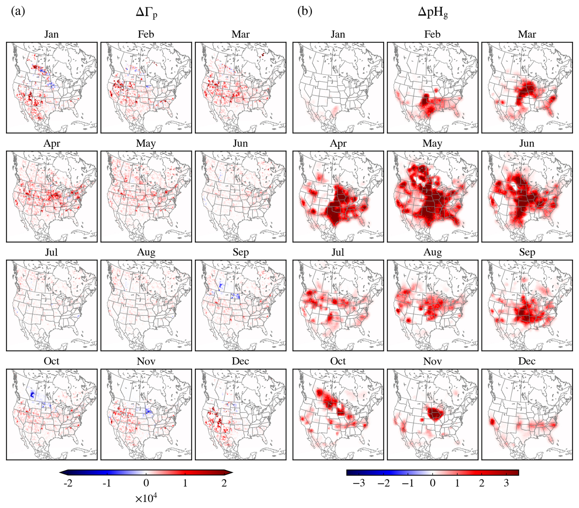
Figure 6 Bidirectional flux model inversions. Panel (a) shows the increments to the ammonium potential source term Γ_p, while (b) shows the pH_g increments.

The largest increments for pH_g occur in the central US and Canada for April to June, where the increment reaches values of 3.5, resulting in total pH_g values of 8.5. Although the increments for pH_g are generally more concentrated in the middle of North America as compared to the increments for Γ_p, large pH_g increments do occur along the East coast of North America and in California's Central Valley in the spring and summer. The pH_g increments are also generally more spread out spatially and smoother as compared to the Γ_p increments.

8.2 Effect of Inversions on the Flux Model and Emissions

With the inversions described in the previous sections, GEM-MACH was run with the revised parameters for the bidirectional flux model, as well as with the unidirectional flux models for comparison. For the unidirectional flux run, emissions are set so that their monthly means are equal to those in the bidirectional flux run (instead of the inventory values to have the benefit of the inversions), but its intramonthly emissions time profiles are set using the unidirectional scheme as described in Sect. 3.

The monthly mean values for the ammonia ground emissions potential Γ_g and the time constant τ_a from GEM-MACH using the inversion-derived bidirectional flux parameters are shown in Fig. 7. The values displayed in this figure are the weighted means across the 15 land-use categories in the model. Regions with significant agriculture and consequently ammonia emissions, such as California's Central Valley, the Canadian prairies, the midwestern US, and North Carolina, can have ground emissions potential values ranging from 10⁴ to 5×10⁴. Ground emission potential values vary greatly with ground condition, vegetation type, and (if applied) fertilizer type and time since application. Reported ground emission potential values for fertilized ground range between 10³ and 10⁶ (Massad et al., 2010), placing the higher end of the inversion values for Γ_g roughly at the midpoint of this range (in terms of the order of magnitude).

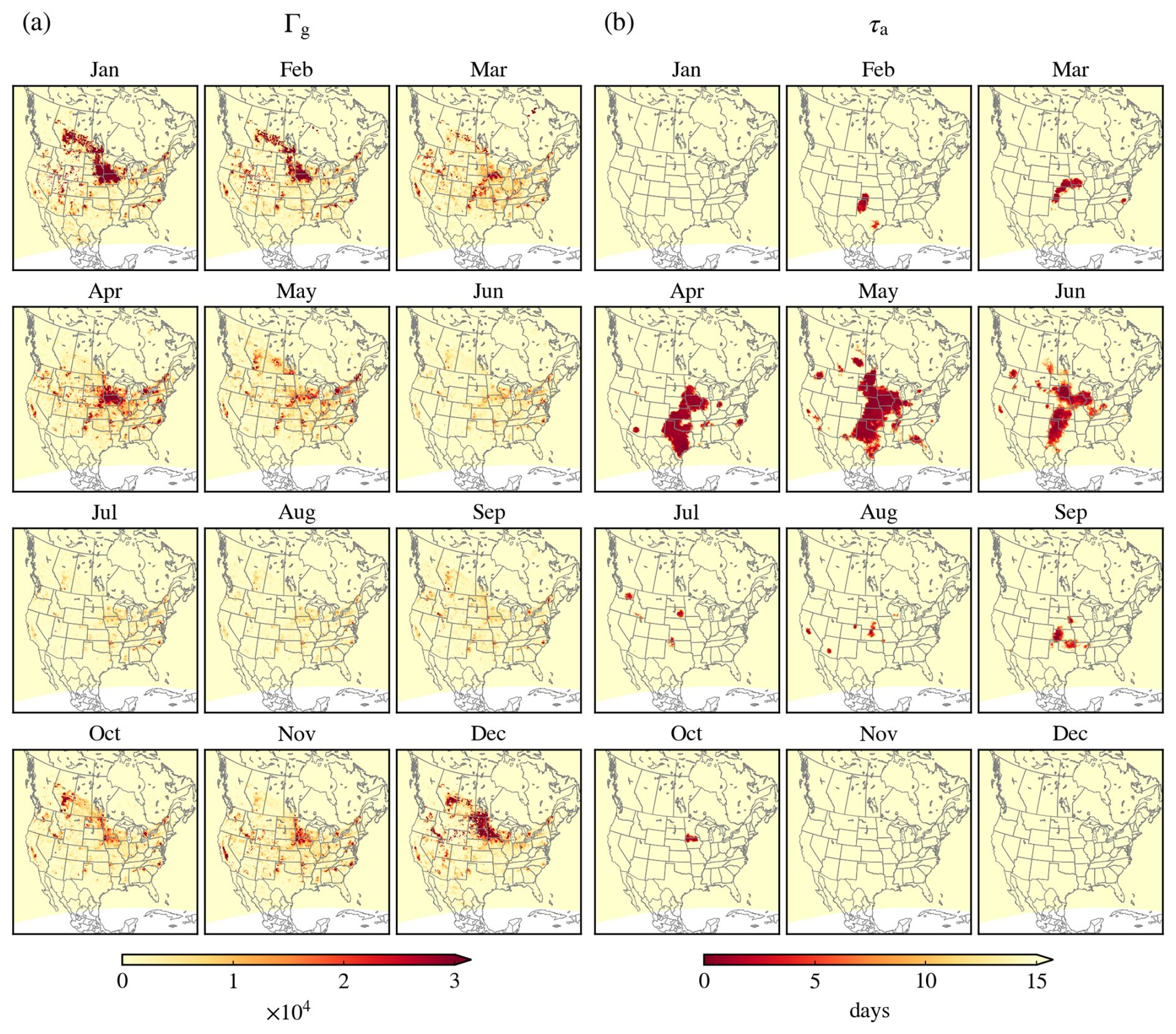
Figure 7 Monthly mean values for (a) the ammonia ground emissions potential Γ_g and (b) the time constant τ_a from the bidirectional flux model with parameters set from the inversions. Values are the weighted mean over land-use categories.

We expect the atmospheric ammonia concentrations to have a non-negligible influence on the emissions potential when τ_a≲τ_p. From Fig. 7b, we can see that the inversions place τ_a at or below τ_p=3 d for large swaths of the central US for April to June, as well as some smaller regions within the model domain. In these regions, the emissions potential will equilibrate with the atmospheric ammonia concentrations within hours to days, while the regions with τ_a≫3 d will have emissions potentials that are approximately static within each month and will be relatively insensitive to the atmospheric ammonia levels.

The changes in the monthly mean ammonia emissions when GEM-MACH is run with the bidirectional flux model with Γ_p and pH_g set from the inversions as compared to using their background values are displayed in Fig. 8. Changes in the emissions are most significant from March to October. Emissions increases exceeding 5 kg ha⁻¹ can be seen in the Central Valley, the American midwest, and northern Texas, which represent increases of over 80 % as compared to the case without inversions (see Fig. S3 in the Supplement for plots of the monthly mean emissions with and without the inversions). Although overall the inversions increase emissions, significant decreases can be seen in some regions, such as a decrease of 2.6 kg ha⁻¹ in North Dakota in September (∼60 % decrease) and a decrease of 4.5 kg ha⁻¹ (∼96 % decrease) in southern California in April.

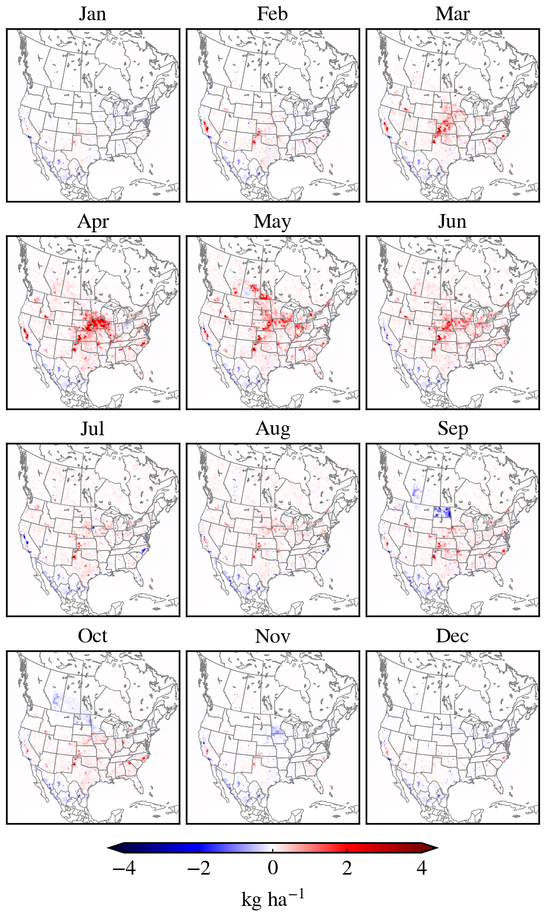
Figure 8 Changes in the monthly mean ammonia emissions from the bidirectional flux model using parameters Γ_p and pH_g from inversions as compared to using their (inventory-derived) background values.

Many of the regions where the inversions give large changes to Γ_p results in significant changes in emissions, but there are a few regions where this is not the case, most notably for the significant increase to Γ_p in Alberta and Saskatchewan in January (seen in Fig. 6a) that do not produce sizable changes in the ammonia emissions (shown in Fig. 8). This is primarily due to the strong temperature dependence of χ_s, as seen in Eq. (5), so that the same value of Γ_g may result in significantly fewer emissions in the winter as compared to the warmer seasons.

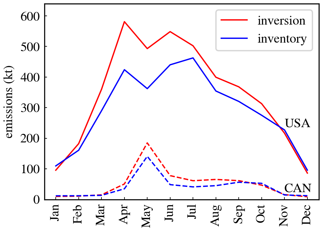
Figure 9 Total ammonia emissions for the continental United States (USA; solid lines) and Canada (CAN; dashed lines) from the inversions (red curves) and the emissions inventory (blue curves).

Figure 9 shows the total emissions over the continental United States and Canada from the inversions along with inventory emissions for comparison. In the winter months, when ammonia emissions are low, the emissions from the inversions are close to the inventory emissions. For April to September, the total emissions from the inversions increase between 9 % and 61 % in Canada and between 9 % to 41 % in the continental United States, with the largest total increases occurring in April for the continental United States and in May for Canada, which is generally the start of the crop growing season when fertilizer is applied to fields.

8.3 Differences In Ammonia Concentrations Between Flux Models

We now turn our attention to comparing the resulting atmospheric ammonia concentrations from the unidirectional and bidirectional flux models. For the remainder of this section, all results presented for both the unidirectional and bidirectional flux models use inversion-derived parameters (as opposed to inventory-derived parameters).

Figure 10 shows the root mean square differences in ammonia surface concentrations between the unidirectional and bidirectional flux model runs. Significant differences between the flux schemes are seen in the midwestern US, the Central Valley, the Eastern seaboard, and Canadian Prairies during the spring, summer, and fall. A number of regions have large root mean square difference on the order of 10 ppbv. For comparison, the monthly mean ammonia surface concentrations for the unidirectional model generally vary between 0.5 and 30 ppbv (see Fig. S4). The root mean square differences between flux models exceeds 50 % in many regions and can range from 100 % to 150 % in the Central Valley during the spring (in comparison to the monthly mean unidirectional values).

Figure 10 Root mean square differences in ammonia surface concentrations between the unidirectional and bidirectional flux models, both of which use inversion-derived parameters.

8.4 Comparison with Surface Observations

The previous section examined the differences in surface concentrations between the unidirectional and bidirectional flux models using parameters set via inversions. We now compare these model results with the ammonia surface observations described in Sect. 6.2.

Figure 11 shows the differences in RMSE values for surface ammonia observations from AMoN and NAPS stations for the unidirectional and bidirectional flux model runs, taken over all months in 2016. Red markers indicate that the RMSE for the bidirectional run is smaller than for the unidirectional run and blue markers indicate larger RMSE values for the bidirectional run. Statistically significant/insignificant differences at a confidence level of 1σ≈68.2 % are denoted by circular/square markers in this figure. Out of the 113 stations in the combined AMoN and NAPS dataset, 28 stations show a statistically significant improvement in the RMSE for the bidirectional run, most of which are on the East coast or American midwest. Four stations show statistically significant increases in RMSE from using the bidirectional flux model. The median station RMSE for the unidirectional run of 38 % decreases to 32 % for the bidirectional run. The statistically significant changes in RMSE range from decreases of 82 % to increases of 31 %.

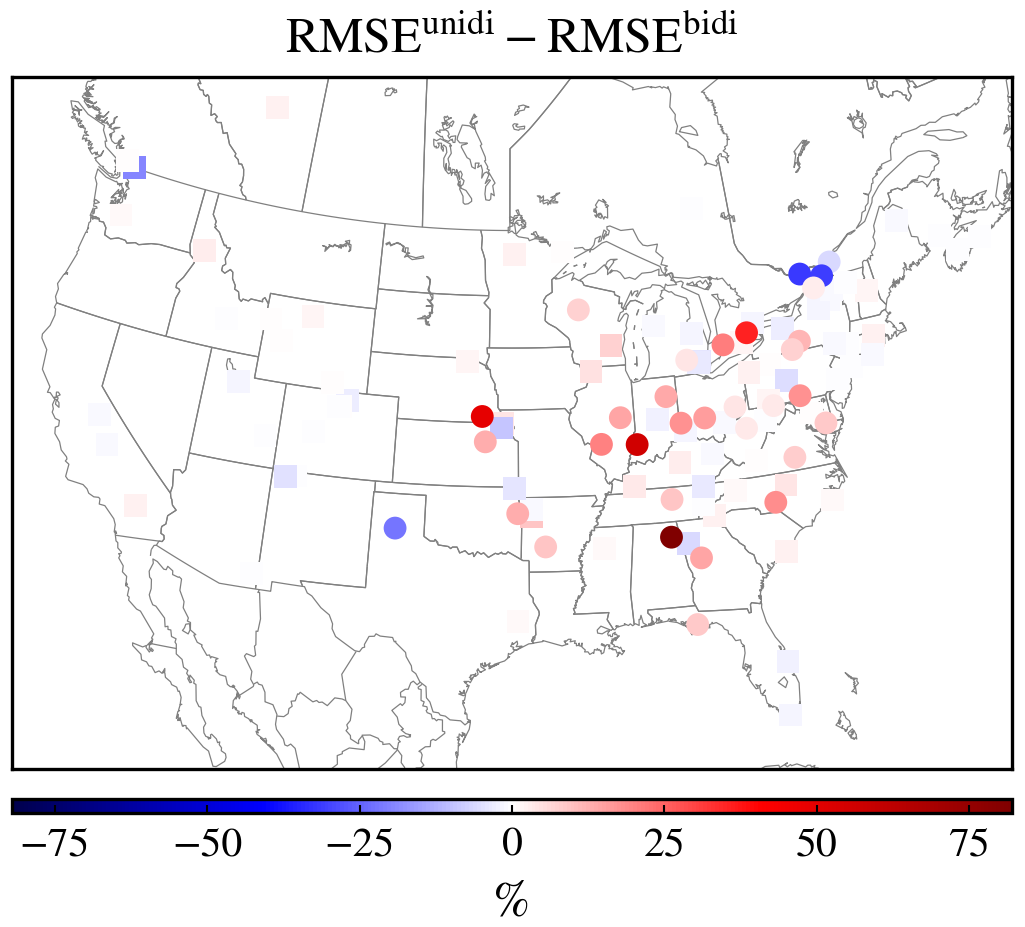
Figure 11 Difference in RMSE values between the unidirectional (RMSE^unidi) and bidirectional (RMSE^bidi) flux models for surface ammonia observations from AMoN and NAPS stations for 2016. Both flux models use inversion-derived parameters. Differences that are statistically significant/insignificant at the 1σ confidence level are shown with a circular/square markers.

The changes in bias, error standard deviation, correlation, and root mean square error between the unidirectional and bidirectional runs for the AMoN and NAPS ammonia surface observations are illustrated in Fig. 12. Red upward-pointing triangles indicate an improvement in the statistic (a reduction for bias, STDE, and RMSE, an increase for ρ) for the bidirectional flux model as compared to the unidirectional flux model. Blue downward-pointing triangles indicate a degradation in the statistic (an increase for bias, STDE, and RMSE, a decrease for ρ) for the bidirectional flux model run as compared to the unidirectional flux model. Filled triangles indicate that the change in the statistic is statistically significant at the 1σ confidence level. Statistics are compiled for each month individually as well as for the whole year. These statistics can be found in full in Tables S1 and S2 of the Supplement.

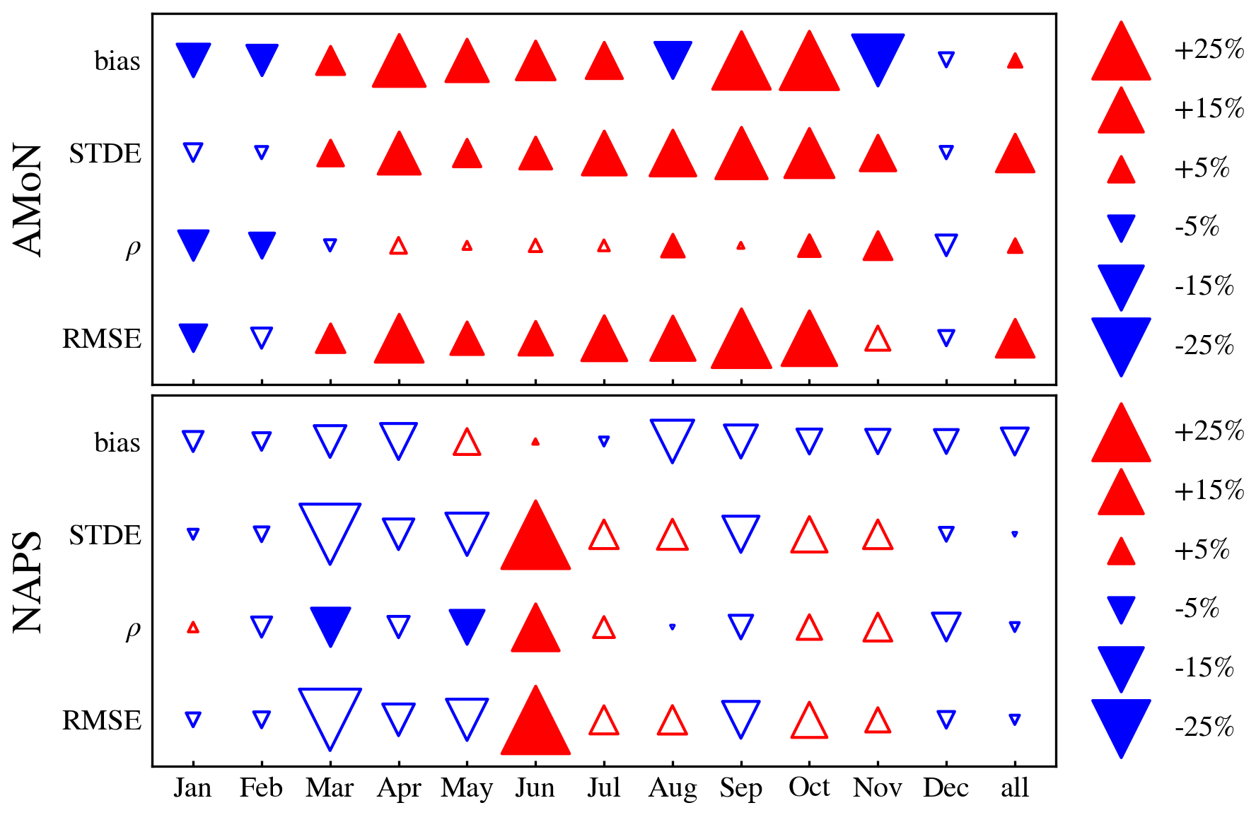
Figure 12 Changes in validation statistics with respect to AMoN (top) and NAPS (bottom) ammonia observations for the bidirectional flux model run as compared to the unidirectional model. Both flux models use inversion-derived parameters. Red upward-pointing triangles indicate an improvement in the statistic (a reduction for bias, STDE, and RMSE, an increase for ρ) for the bidirectional model as compared to the unidirectional model, while blue downward-pointing triangles indicate a degradation in the statistic (an increase for bias, STDE, and RMSE, a decrease for ρ). The size of the triangle indicates the magnitude of the change in the statistic, where the percentages in the legend are in reference to the observation mean for the bias, STDE, and RMSE, and for ρ is in reference to a value of one (e.g. a change of +5 % for ρ indicates that ρ increased by 0.05). Filled triangles indicate that the change in the statistic is statistically significant at the 1σ confidence level. “all” in the x-axis refers to the whole year of 2016.

For AMoN, the top panel of Fig. 12 shows that the bias decreases for March to July and for September and October for the bidirectional model run as compared to unidirectional model. In these months, the bias for the unidirectional model ranges from 13 % to 50 %, but is between 14 % and 26 % for the bidirectional model (see Table S1 for all values and uncertainties). A statistically significant degradation of the bias is seen for January, February, August, and November. The bidirectional model reduces the bias taken over the whole year by 1.4 %. The unidirectional model has error standard deviations that range from 53 % to 193 %, which are reduced in the bidirectional run for March to November (second row from the top in Fig. 12), with the reductions ranging from 5 % to 20 %, and is reduced by 11 % over the year. While the bidirectional run degrades the error standard deviations in January, February and December, these changes are not statistically significant (as indicated by the unfilled triangles). Some improvements to the correlation ρ can be seen for AMoN (third row from the top in Fig. 12), increasing from 0.62 for the unidirectional model to 0.64 for bidirectional model over the year. The RMSE for the bidirectional model is smaller than for unidirectional model for March to November (although the improvement is not statistically significant for November), and over the whole year the bidirectional model reduces the RMSE value by 11 % (90 % reduced from 101 %) as compared to the unidirectional model.

The bidirectional model improves nearly every statistic for AMoN over the spring, summer, and fall months, as well as over the whole year, but degrades the statistics somewhat in the winter months. This difference in performance during the winter as compared to the rest of the year may be due to the quality of the model's surface temperature (as described in Sect. 2), which for the continental US in 2016 performs worse in the winter than for the rest of the year.

In contrast to AMoN, few differences in the statistics for the NAPS observations between the unidirectional and bidirectional models are statistically significant, as seen in the bottom panel of Fig. 12. The STDE, ρ, and RMSE values for the bidirectional model in June are better than for the unidirectional model, while opposite is true for ρ in March and May, but otherwise the statistics for the different flux models are not significantly different from one another. As seen in Fig. 11, most of the stations that show improvement from using the bidirectional flux model are concentrated in the mid-to-eastern US, where there are stations for AMoN but not NAPS. Overall, the bidirectional flux model improves the agreement of the GEM-MACH model with the ammonia surface observations in the spring, summer, and fall, while degrading the model performance somewhat in the winter.

8.5 Sensitivity of Inversions to Model Parameters

We conclude with a brief examination of the relative sensitivity of the inversions to the inversion model parameters. While there is a noticeable reduction in the posterior uncertainties for both Γ_p and pH_g, the reduction in uncertainties for Γ_p was much larger than that for pH_g in many regions (see Fig. S5). Furthermore, the number of degrees of freedom for the inversions (Rodgers, 2000) associated with Γ_p are 2 to 8 times larger than that associated with pH_g. Overall, the inversions are better able to constrain Γ_p than pH_g.

While the ammonia retrievals from CrIS do constrain Γ_p more than pH_g, including pH_g as an inversion parameter can nonetheless have significant effects on the atmospheric ammonia concentration. Inversions were repeated with β={Γ_p} as the sole inversion field, with the values of pH_g set to values from the WoSIS pH database. The root mean square differences in the ammonia surface concentrations between inversions with β={Γ_p} compared to inversions with $\mathit{\beta }=\mathit{\{}{\mathrm{\Gamma }}_{\mathrm{p}},{\mathrm{pH}}_{\mathrm{g}}\mathit{\}}$ (shown in Fig. S6) can be as large as 10 ppbv in some regions, such as the midwestern US and California's Central Valley, which is comparable to the differences between the unidirectional and bidirectional models (as seen in Fig. 10), although with not as large of a horizontal extent. Including pH_g as an inversion parameter also decreases the biases with AMoN observations in May, June, September, and October, but increases the bias in July and August (see Fig. S7).

9 Conclusions

Atmospheric ammonia plays a central role in particulate matter formation and its deposition to the surface can have detrimental effects on the health of an ecosystem. As ammonia levels have stayed the same or increased in many regions, in contrast to many other pollutants in the atmosphere with declining trends, ammonia has emerged as a pollutant of concern in recent decades. Bottom-up inventories of ammonia emissions, which are primarily from agricultural sources, are often used in air quality forecasting models, but generally have large uncertainties. Recently, there has been an effort to use ammonia retrievals from satellite-borne instruments to improve ammonia emissions inventories. This is most often done by using these retrievals in emissions inversion systems that combine the inventory emissions with the satellite information.

Bidirectional flux models offer a unified scheme for emission and deposition of ammonia that most often have an explicit dependence on local conditions, most notably temperature. While bidirectional flux models have been included in a number of atmospheric chemistry models in the last decade, there have been relatively few studies looking into the ability of ammonia retrievals to constrain the bidirectional flux model parameters.

A novel bidirectional flux model is introduced in this work that was developed for use with inversion systems. This model describes the bidirectional exchange of atmospheric ammonia with the surface, which has an emissions potential that evolves in time according to this exchange. The bidirectional flux model is parametrized to describe this bidirectional exchange while reducing the number of model parameters that satellite retrievals cannot differentiate between. This improves convergence within inversion algorithms and yields a model that is relatively easy to implement and maintain in atmospheric chemistry models.

Inversions using CrIS ammonia retrievals were performed to tune the values for the ammonium source potential and the ground pH in the bidirectional flux model implemented in the GEM-MACH air quality model. In areas with significant agriculture, the inversions yielded ground emissions potentials in the range of 10⁴ to 5×10⁴. From the inversions, the values for the time constant for equilibration between the atmosphere and the ground ammonium pool were below a week for large regions in the midwestern and southern US in the spring and summer. In these regions, the ground ammonium concentration can change rapidly in response to atmospheric ammonia levels. The inversions increase ammonia emissions in most regions within the model domain, with some regions nearly doubling their emissions, although significant emissions decreases are seen in some regions for certain months. Overall monthly ammonia emissions in Canada and the continental US are increased between 9 % and 61 % in the spring/summer/fall.

Unidirectional and bidirectional ammonia flux models with parameters determined via inversions were compared with one another. Significant differences in ammonia emissions between unidirectional and bidirectional models were seen in locations with large agricultural industries, such as California's Central Valley, North Carolina, and the Canadian Prairies. In these regions, ammonia surface concentrations can vary between models on the order of 10 ppbv, corresponding to a variation of 50 % to 150 %.

When compared to surface observations, the bidirectional flux model improves the agreement between the surface ammonia field from GEM-MACH and observations from the AMoN network as compared to the unidirectional model in the spring, summer, and fall, although worsens the agreement somewhat in the winter. In the spring/summer/fall months, the bidirectional model decreased the bias with AMoN observations between 14 % and 26 % as compared to the unidirectional model, and decreased the error standard deviation between 5 % to 20 %. The stations with the most significant improvement were in the American midwest and near the North American east coast. Few statistically significant changes between unidirectional and bidirectional models were observed in the NAPS network due to the number and placement of these stations. Future evaluations could extend these validations by including comparisons to ammonium wet deposition observations to provide an additional validation data set.

Appendix A: Details of the Capacitance Model

This section contains details of the derivations in Sects. 4.1 and 5.2. The flux F_t at the top of the surface layer is given by

$$\begin{array}{}\text{(A1)}& F_{\mathrm{t}}={\displaystyle \frac{{\mathit{\chi }}_{\mathrm{c}}-{\mathit{\chi }}_{\mathrm{a}}}{R_{\mathrm{a}}+R_{\mathrm{b}}}}=\sum _{i=\mathrm{1}}^{N_{\mathrm{c}}}{\displaystyle \frac{{\mathit{\chi }}_{\mathrm{s}}^{\left(i\right)}-{\mathit{\chi }}_{\mathrm{c}}}{R_{\mathrm{c}}^{\left(i\right)}}}={\displaystyle \frac{{\mathit{\chi }}_{\mathrm{s}}-{\mathit{\chi }}_{\mathrm{c}}}{R_{\mathrm{c}}}},\end{array}$$

where the second equality follows from using Kirchhoff's first law at the junction χ_c and the third equality follows from the definitions of R_c and χ_s in Eqs. (1a) and (1b), respectively. Using the expression above, we can solve for the canopy compensation point χ_c as

$$\begin{array}{}\text{(A2)}& {\mathit{\chi }}_{\mathrm{c}}={\displaystyle \frac{R_{\mathrm{c}}}{R_{\mathrm{t}}}}{\mathit{\chi }}_{\mathrm{a}}+\left(\mathrm{1}-{\displaystyle \frac{R_{\mathrm{c}}}{R_{\mathrm{t}}}}\right){\mathit{\chi }}_{\mathrm{s}}.\end{array}$$

Substituting Eq. (A2) back into Eq. (A1) then gives Eq. (2).

Now using Eqs. (A2) and (1b) in Eq. (8) yields

$$\begin{array}{}\text{(A3)}& \begin{array}{rl}{\displaystyle \frac{\mathrm{d}{Q}_{\mathrm{g}}}{\mathrm{d}t}}& ={\displaystyle \frac{\mathrm{1}}{R_{\mathrm{t}}}}{\displaystyle \frac{R_{\mathrm{c}}}{R_{\mathrm{g}}}}\left[{\mathit{\chi }}_{\mathrm{a}}+\left({\displaystyle \frac{R_{\mathrm{t}}}{R_{\mathrm{g}}}}-{\displaystyle \frac{R_{\mathrm{c}}}{R_{\mathrm{g}}}}-{\displaystyle \frac{R_{\mathrm{t}}}{R_{\mathrm{c}}}}\right){\mathit{\chi }}_{\mathrm{g}}\right]+{\displaystyle \frac{{\mathit{\chi }}_{\mathrm{p}}-{\mathit{\chi }}_{\mathrm{g}}}{R_{\mathrm{p}}}}\\ & ={\displaystyle \frac{\mathrm{1}}{R_{\mathrm{t}}}}{\displaystyle \frac{R_{\mathrm{c}}}{R_{\mathrm{g}}}}\left[{\mathit{\chi }}_{\mathrm{a}}-{\mathit{\chi }}_{\mathrm{g}}+\left(\mathrm{1}-{\displaystyle \frac{R_{\mathrm{c}}}{R_{\mathrm{g}}}}+{\displaystyle \frac{R_{\mathrm{t}}}{R_{\mathrm{g}}}}-{\displaystyle \frac{R_{\mathrm{t}}}{R_{\mathrm{c}}}}\right){\mathit{\chi }}_{\mathrm{g}}\right]\\ & +{\displaystyle \frac{{\mathit{\chi }}_{\mathrm{p}}-{\mathit{\chi }}_{\mathrm{g}}}{R_{\mathrm{p}}}}\\ & ={\displaystyle \frac{\mathrm{1}}{R_{\mathrm{t}}}}{\displaystyle \frac{R_{\mathrm{c}}}{R_{\mathrm{g}}}}({\mathit{\chi }}_{\mathrm{a}}-{\mathit{\chi }}_{\mathrm{g}})+{\displaystyle \frac{\mathrm{1}}{R_{\mathrm{t}}}}{\displaystyle \frac{R_{\mathrm{c}}}{R_{\mathrm{g}}}}\left(\mathrm{1}-{\displaystyle \frac{R_{\mathrm{c}}}{R_{\mathrm{g}}}}\right)\left(\mathrm{1}-{\displaystyle \frac{R_{\mathrm{t}}}{R_{\mathrm{c}}}}\right){\mathit{\chi }}_{\mathrm{g}}\\ & +{\displaystyle \frac{{\mathit{\chi }}_{\mathrm{p}}-{\mathit{\chi }}_{\mathrm{g}}}{R_{\mathrm{p}}}}\\ & ={\displaystyle \frac{\mathrm{1}}{R_{\mathrm{t}}}}{\displaystyle \frac{R_{\mathrm{c}}}{R_{\mathrm{g}}}}({\mathit{\chi }}_{\mathrm{a}}-{\mathit{\chi }}_{\mathrm{g}})+{\displaystyle \frac{\mathrm{1}+\mathit{\alpha }}{R_{\mathrm{p}}}}\left({\displaystyle \frac{{\mathit{\chi }}_{\mathrm{p}}}{\mathrm{1}+\mathit{\alpha }}}-{\mathit{\chi }}_{\mathrm{g}}\right),\end{array}\end{array}$$

where α is defined in Eq. (11). Using $Q_{\mathrm{g}}={\mathrm{\Gamma }}_{\mathrm{g}}h\left[{\mathrm{H}}^{+}\right]$ and assuming h[H⁺] is constant in time then gives

$$\begin{array}{}\text{(A4)}& \begin{array}{rl}{\displaystyle \frac{\mathrm{d}{\mathrm{\Gamma }}_{\mathrm{g}}}{\mathrm{d}t}}& ={\displaystyle \frac{\mathrm{1}}{R_{\mathrm{t}}}}{\displaystyle \frac{R_{\mathrm{c}}}{R_{\mathrm{g}}}}{\displaystyle \frac{{\mathit{\chi }}_{\mathrm{a}}-{\mathit{\chi }}_{\mathrm{g}}}{h\left[{\mathrm{H}}^{+}\right]}}+{\displaystyle \frac{\mathrm{1}+\mathit{\alpha }}{R_{\mathrm{p}}}}{\displaystyle \frac{\frac{{\mathit{\chi }}_{\mathrm{p}}}{\mathrm{1}+\mathit{\alpha }}-{\mathit{\chi }}_{\mathrm{g}}}{h\left[{\mathrm{H}}^{+}\right]}}\\ & ={\displaystyle \frac{\mathrm{1}}{R_{\mathrm{t}}C}}{\displaystyle \frac{R_{\mathrm{c}}}{R_{\mathrm{g}}}}({\mathrm{\Gamma }}_{\mathrm{a}}-{\mathrm{\Gamma }}_{\mathrm{g}})+{\displaystyle \frac{\mathrm{1}+\mathit{\alpha }}{R_{\mathrm{p}}C}}({\mathrm{\Gamma }}_{\mathrm{p}}-{\mathrm{\Gamma }}_{\mathrm{g}}),\end{array}\end{array}$$

where we have used Eqs. (5), (7), (10a), and (10b) in the last line. Using the RC time constants in Eqs. (12a) and (12b) in the equation above then yields the prognostic equation for Γ_g given in Eq. (9).

Appendix B: Statistics Used for Comparisons to Surface Observations

When comparing GEM-MACH model results to surface observations, the bias, standard deviation of errors (STDE), root mean square error (RMSE), and Pearson correlation coefficient (ρ) between the surface observations and model are defined as

$$\begin{array}{}\text{(B1a)}& {\displaystyle }\mathrm{bias}=\stackrel{\mathrm{‾}}{M}-\stackrel{\mathrm{‾}}{O},\text{(B1b)}& {\displaystyle }\mathrm{STDE}=\sqrt{{\displaystyle \frac{\mathrm{1}}{N-\mathrm{1}}}\sum _i^N(M_i-\stackrel{\mathrm{‾}}{M}-O_i+\stackrel{\mathrm{‾}}{O}{)}^{\mathrm{2}}},\text{(B1c)}& {\displaystyle }\mathrm{RMSE}=\sqrt{{\displaystyle \frac{\mathrm{1}}{N}}\sum _i^N(M_i-O_i{)}^{\mathrm{2}}},\text{(B1d)}& {\displaystyle }\mathit{\rho }={\displaystyle \frac{{\sum }_i^N(M_i-\stackrel{\mathrm{‾}}{M})(O_i-\stackrel{\mathrm{‾}}{O})}{\sqrt{{\sum }_i^N(M_i-\stackrel{\mathrm{‾}}{M}{)}^{\mathrm{2}}}\sqrt{{\sum }_i^N(O_i-\stackrel{\mathrm{‾}}{O}{)}^{\mathrm{2}}}}},\text{(B1e)}& {\displaystyle }\stackrel{\mathrm{‾}}{O}={\displaystyle \frac{\mathrm{1}}{N}}\sum _i^N{O}_i,\text{(B1f)}& {\displaystyle }\stackrel{\mathrm{‾}}{M}={\displaystyle \frac{\mathrm{1}}{N}}\sum _i^N{M}_i,\end{array}$$

where O_i is the ith observation out of N observations and M_i is its corresponding GEM-MACH model value. When the bias, STDE, or RMSE are given as a percentage, the denominator is the annual mean observation value.