Development of a next-generation general ocean circulation model for the Great Lakes

The Laurentian Great Lakes share several physical characteristics with the coastal ocean, including atmosphere–water interactions, rotational dynamics, and ice cover processes. However, their weak density stratification, relatively small surface area, and distinct seasonal mixing cycles pose unique challenges for numerical modeling. Modeling approaches and parameterizations developed for global applications, however, may yet provide valuable pathways for addressing persistent biases in lake models. To examine these possibilities, we develop a 3D hydrodynamic model for Lake Michigan-Huron (LMH) using the Modular Ocean Model version 6.0 coupled with the Sea Ice Simulator version 2.0 (MOM6-SIS2). Originally designed for global ocean and earth system modeling, MOM6 offers flexible vertical coordinate systems (VCSs) to maintain density gradients and improved handling of complex bathymetry, both potential advantages for application in inland water bodies like the Great Lakes. This is the first study to investigate MOM6-SIS2's ability to simulate key features of hydrography and circulation in freshwater systems under different VCSs. This study tested z^∗ (depth-based) and hybrid (depth and isopycnal) VCSs. Simulations were performed for the years 2017 and 2018 and evaluated against in situ and remote sensing observations, as well as outputs from a contemporary Finite Volume Community Ocean Model (FVCOM) of LMH (LMH-FVCOM), used in an operational forecast system. MOM6-SIS2-LMH skillfully simulated daily averaged lake surface temperature (LST), vertical thermal structure, and ice concentration, with biases in LST and ice concentration generally below 0.5 °C and 2 %, respectively. It also produced comparable results to LMH-FVCOM in terms of LST, vertical thermal structure, and ice concentration. Both VCSs (z^∗ and hybrid) successfully captured large-scale circulation patterns and seasonal overturning. The hybrid VCS, reduced excessive thermocline diffusion in deep waters, observed in both FVCOM and MOM6-SIS2 with z^∗ VCS and allowed the model to maintain ecologically important deep cold water in the summer months. These improvements highlight the potential of MOM6-SIS2 to successfully simulate lake dynamics and offer the potential to more accurately resolve the delicate balance of thermal structure and mixing in stratified lake environments. However, the limited nearshore resolution resulting from MOM6's structured grid degraded the simulation of flows through the Straits of Mackinac, as well as nearshore temperature and water level variability.

1 Introduction

One of the primary challenges in applying global ocean models to lakes is the difference between the modeling approaches and parameterizations most commonly used by the large-scale ocean and lake/estuarine modeling communities. Many large-scale ocean models, such as the Modular Ocean Model version 6.0 (MOM6; Adcroft et al., 2019), Nucleus for European Modelling of the Ocean version 3.6 (NEMO3.6; Gurvan et al., 2017), Miami Isopycnal Coordinate Model (MICOM; Bleck et al., 1992), employ structured horizontal grids and have moved toward density based (isopycnal), and hybrid (depth and density) vertical coordinate systems (VCSs). These frameworks are well suited for simulating the circulation in deep, stratified, and horizontally extensive ocean basins. Isopycnal and hybrid VCSs have, for example, helped address overly diffuse ocean thermoclines common in earlier depth-based models (Adcroft et al., 2019). They have also improved preservation of climate-critical water masses and overflows (Legg et al., 2006). Structured horizontal grids, meanwhile, have afforded greater computational efficiency at comparable resolution (Ding et al., 2021) and more consistent separation between resolved and sub-grid scale processes that must be parameterized (Staniforth and Thuburn, 2012). These advantages are often deemed to outweigh disadvantages posed by lack of horizontal resolution flexibility and limited vertical resolution in shallow areas with structured/hybrid and structured/isopycnal approaches. Consensus, however, has not been reached and considerable success has also been achieved using unstructured grids and alternative VCSs (e.g., Abdolali et al., 2024; Ye et al., 2018).

In contrast to open ocean systems, lakes and estuaries are shallower, topographically complex, and strongly influenced by localized wind forcing, mixing, and boundary interactions. To capture these dynamics, many lake and estuarine models such as the Finite Volume Community Ocean Model (FVCOM; Chen et al., 2003), Semi-implicit Cross-scale Hydroscience Integrated System Model (SCHISM; Zhang et al., 2016), and the Estuary and Lake COmputer Model (ELCOM; Hodges, 2000) frequently use unstructured grids with terrain-following (sigma) vertical coordinate systems, which allow better representation of nearshore bathymetry, shoreline complexity, and vertical resolution in shallow areas. These advantages, however, may be eroded by the need for bathymetric smoothing (Cai et al., 2022; Prakash et al., 2022) and potential for numerical diffusion when using sigma coordinates (Mellor et al., 1998), and challenges of parameterizing sub-grid scale processes and numerically solving the equations of motion on an uneven grid (Lee et al., 2020). Like global models, efforts to identify the most effective hydrodynamic modeling approaches for estuarine and lake systems remain ongoing (Ganju et al., 2016; Ishikawa et al., 2022).

These fundamental differences in prevailing model approaches and remaining uncertainties highlight the challenges of adapting large-scale ocean models to smaller freshwater systems, yet they may still offer opportunities to mitigate persistent biases in lake modeling. In this study, we assess the capacity of the Modular Ocean Model version 6 – Sea Ice Simulator version 2 (MOM6-SIS2) to simulate critical dynamics of Lake Michigan-Huron (LMH), including lake surface temperature (LST), vertical thermal profile, inertial oscillation periods, seasonal circulation, and ice coverage and thickness. MOM6 uses a structured horizontal grid and offers flexible vertical coordinate options (Adcroft et al., 2019). MOM6-SIS2 was used in Geophysical Fluid Dynamics Laboratory (GFDL)'s CM4, Held et al. (2019) and Earth System Model, ESM4.1, Dunne et al. (2020) contributions to the Sixth Coupled Model Intercomparison Project (CMIP6) and it is also employed in global weather, seasonal, and decadal prediction systems (Delworth et al., 2020). In addition, MOM6-SIS2 has been successfully adapted for various regional shelf-scale ocean modeling applications, demonstrating its versatility across a range of spatial scales (Drenkard et al., 2024; Liao et al., 2025; Ross et al., 2023; Seelanki et al., 2025; Seijo-Ellis et al., 2024).

The novel application of MOM6-SIS2 to the Laurentian Great Lakes (hereafter “Great Lakes”) represents the first adoption of this ocean model framework for a freshwater system with different physical dynamics than the marine systems in which it is traditionally deployed. This study assesses the performance of MOM6-SIS2-LMH against observations, as well as a modified version of the Lake Michigan-Huron Operational Forecast System (LMHOFS; Kelley et al., 2020), which uses the Finite Volume Community Ocean Model (FVCOM; Chen et al., 2003). Hereinafter, referred to as Lake Michigan-Huron Finite Volume Community Ocean Model (LMH-FVCOM). In addition, the study evaluates MOM6-SIS2-LMH under two different VCSs: z^∗ (depth-based) and hybrid (z^∗ and isopycnal). Specifically, it addresses the following questions: (i) How does MOM6-SIS2-LMH perform relative to both observations and LMH-FVCOM?, (ii) How does MOM6-SIS2-LMH performance vary with the choice of VCSs?, (iii) What are the areas where MOM6-SIS2-LMH shows improved performance, and where does it face limitations? This study will serve as a developmental case study to inform other MOM6-SIS2 deployments across the Great Lakes.

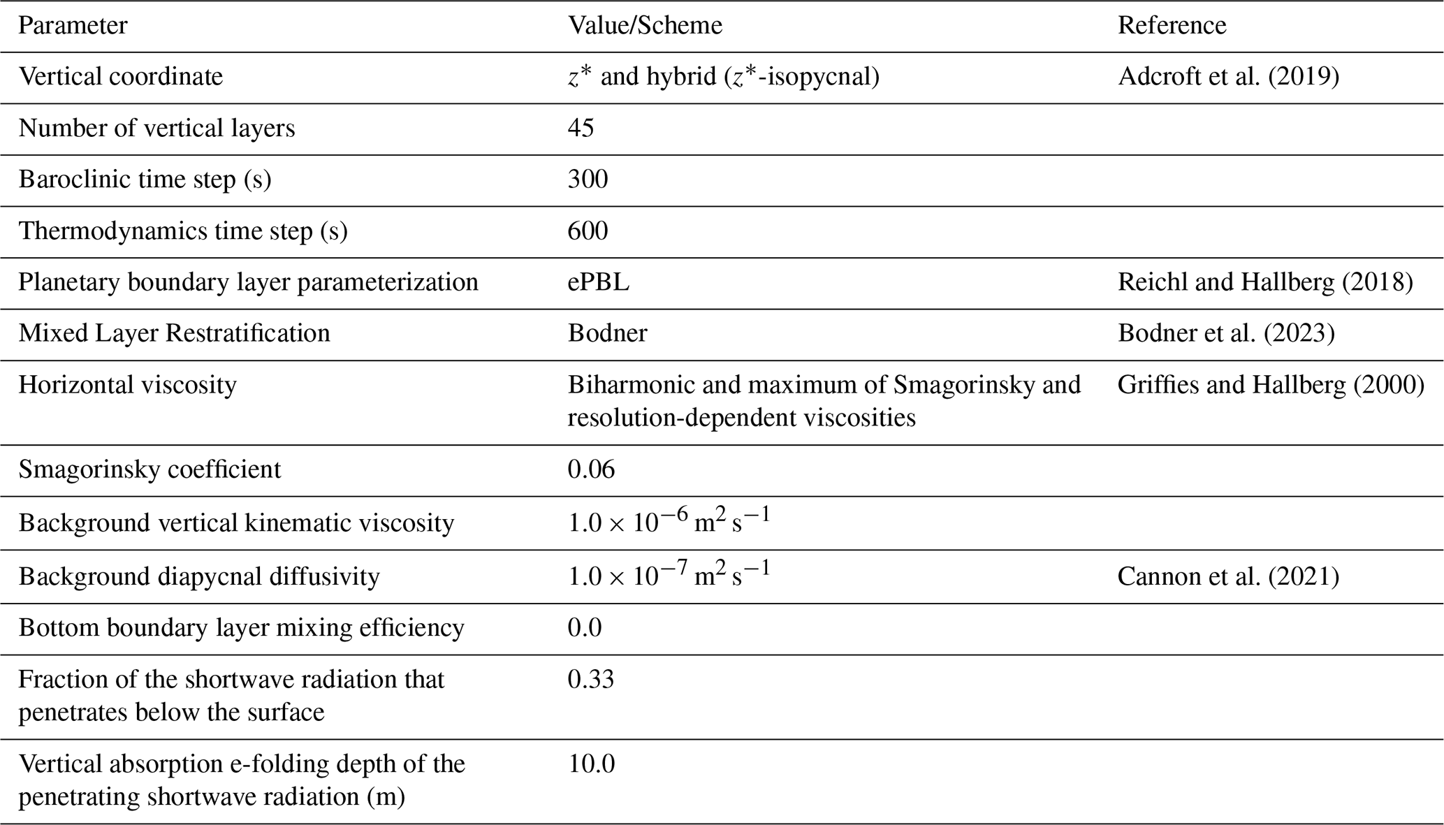
Table 1 Key parameters utilized in the model along with their respective values, as well as supporting references that justify the selection or source of these values.

2 Methods

2.1 Model Description

MOM is a numerical ocean model designed to simulate ocean circulation, ranging from localized process studies to large-scale general circulation forecasts and integration within Earth System Models (ESMs) (Griffies et al., 2015). MOM6 is a three-dimensional ocean circulation model based on the primitive equations, to support both regional and global applications with advanced numerical algorithms (Adcroft et al., 2019). Some of the key features of MOM6 include: (i) the use of a vertical Lagrangian remapping (a variant of the Arbitrary Lagrangian Eulerian (ALE) algorithm) to enable the use of any vertical coordinate, including geopotential (z or z^∗), isopycnal, terrain-following (sigma), or hybrid/user-defined, (ii) ability to handle vanishing layers through its vertical ALE framework making it well suited for accurately simulating dynamic coastal and tidal estuaries, where wetting and drying processes are critical, (iii) a tracer sub-cycling time-stepping scheme that allows for an efficient incorporation of many bio-geochemical constituents. Sea ice is modelled using the Sea Ice Simulator version 2 (SIS2; Adcroft et al., 2019), which employs five sea-ice thickness categories without an explicit ridging scheme. The model uses an elastic-viscous-plastic rheology Hibler III (1979), and a directionally split, piecewise constant advection scheme for ice thickness. Radiative transfer within the ice is handled using the delta-Eddington scheme, and internal thermodynamics follow an enthalpy-conserving approach (Briegleb and Light, 2007). It is important to note that although ice salinity was set to zero to approximate freshwater conditions, the physical parameterizations such as rheology and ice strength were designed for sea ice and have not been modified for lake ice.

2.1.1 Horizontal and vertical grids and resolution

The MOM6-SIS2-LMH employs an Arakawa C grid in the horizontal direction (Arakawa and Lamb, 1977), with a resolution of 1 km, consisting of 730 by 550 grid cells (total cells: 401 500; total lake cells: 124 290). The model bathymetry was referenced to the International Great Lakes Datum (IGLD, 1985). This study tested continuous z^∗ and a hybrid VCS, which has been used in the GFDL OM4 global ocean model Adcroft et al. (2019), and has been configured, as described below, for the lake application herein. For the continuous z^∗ (a height coordinate that is rescaled with the free surface configuration; Adcroft and Campin, 2004), and hybrid (z^∗ and isopycnal; (Adcroft et al., 2019; Bleck, 2002)) VCSs, the model uses 45-layers. For the continuous z^∗ coordinate, the vertical resolution is finest (2 m) from the surface to 30 m depth and from there gradually increases with depth to a maximum thickness of 30 m. The hybrid vertical coordinate system used in MOM6 is based on the approach introduced by Bleck (2002), with a detailed description of this configuration provided by Adcroft et al. (2019). The hybrid VCS defines the vertical grid using either isopycnal layers based on prescribed target densities and/or fixed depths based on the z^∗ coordinate. This allows the vertical grid to evolve in space and time to maintain sufficient resolution in stratified and isothermal waters. The 45 target densities for the isopycnal component ranged from 995 to 1000 kg m⁻³. Target densities were selected based on the expected lake surface temperatures, with a maximum density of 1000 kg m⁻³ at the temperature of maximum density for freshwater (T = 4 °C) and a minimum density of 995 kg m⁻³ at 30 °C. A higher density resolution (∼ 0.03 kg m⁻³) was used between 999.24 and 999.75 kg m⁻³ to better represent thermocline temperatures, approximately 10 to 14 °C. We used the previously described 45-layer z^∗ coordinate as the fixed depths. A schematic illustrating the temperature changes over time for 2017 and the position of interfaces in the water column for z^∗ and hybrid VCSs at a thermistor string station in southern Lake Michigan are shown in Fig. S1 in the Supplement.

The parameter values listed in Table 1 were selected based on established MOM6-SIS2 configurations for regional ocean applications and were refined to ensure physical realism and numerical stability in freshwater environments. Turbulence and mixing parameters were chosen in accordance with studies addressing mixed-layer and boundary-layer dynamics in stratified systems, ensuring appropriate vertical mixing and thermocline formation (Cannon et al., 2021; Reichl and Hallberg, 2018). The reference pressure was set to 1.0 × 10⁵ Pa (10 dbar), corresponding to standard atmospheric conditions and providing a consistent baseline for computing freshwater density.

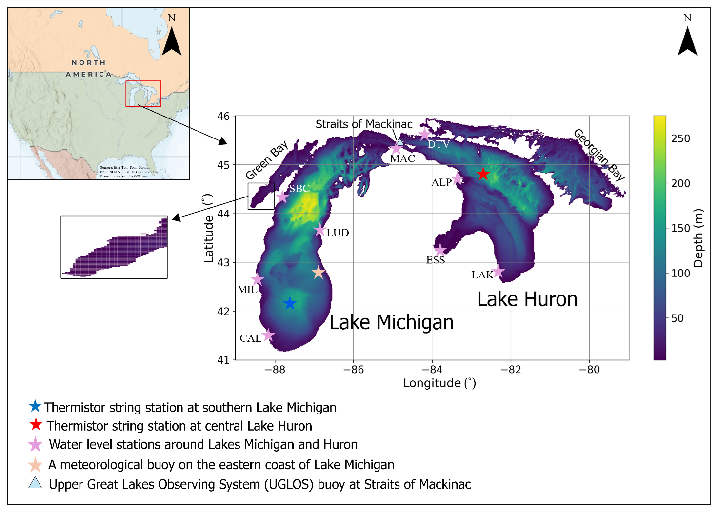
Figure 1 Study area showing bathymetry, with an inset diagram highlighting the structured horizontal grid used for model computations. Thermistor strings, buoy on the eastern coast of Lake Michigan, and water level stations used for validation are shown with coloured stars. The Upper Great Lakes Observing System (UGLOS) buoy at Straits of Mackinac is shown in blue triangle. The labels for the water level stations are defined as follows, CAL – Calumet Harbor, MIL – Milwaukee, LUD – Ludington, SBC – Sturgeon Bay Canal, MAC – Mackinaw City, DTV – De Tour Village, ALP – Alpena, ESS – Essexville, LAK – Lakeport. (Inset diagram source: Esri, TomTom, FAO, USGS | Powered by Esri).

2.1.2 Time Integration

The model is integrated forward in time with a split explicit method (Hallberg and Adcroft, 2009). MOM6 allows for different time steps to be used for various ocean processes: it separates the time stepping of barotropic and baroclinic ocean dynamics from that used for tracer advection, thermodynamics, mixing, and coupled ocean biogeochemistry (Ross et al., 2023). The ocean equations are advanced over the thermodynamic time step using a purely Lagrangian approach in the vertical direction, meaning each layer maintains its volume, although tracers can still transfer between layers via diffusion. This thermodynamic time step is used to update thermodynamic variables and is set as an integer multiple of the shorter baroclinic-dynamics time step, which is used to sub-cycle the momentum and continuity equations. Once the ocean state has been advanced using the Lagrangian framework, a new vertical grid is constructed, and the updated ocean state is remapped onto this new grid (Adcroft et al., 2019).

2.1.3 Model domain

In this study, Lakes Michigan and Huron were treated as a single lake (Fig. 1). Although these lakes are often discussed separately, they are hydrologically considered a single water body due to their shared water level, which is facilitated through their connection via the Straits of Mackinac. For this initial configuration of MOM6-SIS2-LMH, similar to previous model simulations, Cannon et al. (2023), the lake domain is closed at its lateral and bottom, with no river inflows or groundwater exchange. Currents in the Great Lakes are driven primarily by wind and rotation (e.g. Beletsky et al., 1999), and rivers in Lake Michigan-Huron are only expected to influence dynamics relatively close to the outlet of each stream or connecting channel (e.g. St Mary's River and St Clair River). As such, this assumption is not expected to influence discussions in the current study, which are focused on lake wide flow and stratification patterns. Evaporation and precipitation are included through the atmospheric surface forcing; however, because lateral freshwater fluxes are not represented, a spatially uniform correction is applied to the net surface freshwater flux to prevent long-term drift in lake level.

2.1.4 Atmospheric forcing and initial conditions

The model was forced using the hourly European Center for Medium-range Weather Forecasts reanalysis 5th generation (ERA5; Hersbach et al., 2020). Previous studies have used ERA5 reanalysis data to force regional ocean models developed with MOM6-SIS2 (Drenkard et al., 2024; Liao et al., 2025; Ross et al., 2023), and it has also proven to be a viable forcing dataset for other Great Lakes hydrodynamic models (e.g. Abdelhady et al., 2025a, b). MOM6-SIS2-LMH experiments were also run using North American Regional Reanalysis (NARR; Mesinger et al., 2006), but ERA5 was ultimately selected due an overestimation of downward shortwave radiation in NARR (identified from preliminary investigations) that notably biased modeled LST. NARR-forced experiments exhibited a systematic positive bias in downward shortwave radiation (approximately 30 %), which resulted in a consistent warm bias in lake-wide surface temperature, particularly during spring and summer. This bias propagated through the surface heat budget, degrading the agreement with observed temperature variability relative to ERA5-forced simulations (Fig. S2 in the Supplement). In contrast, ERA5 provided a more balanced representation of surface heat flux components and improved overall consistency with observed lake-wide thermal conditions. Therefore, ERA5 was selected as the primary atmospheric forcing dataset for this study. The MOM6-SIS2-LMH models (z^∗ and hybrid VCSs) were initialized from 1 January 2016, using a uniform temperature (T = 4 °C) and velocity (U = 0; V = 0) field. The models were run from 2016 through 2018. Output from the first year (2016) was considered a spin-up period and excluded from subsequent analyses. Although a one-year spin-up period is relatively short compared to requirements for global ocean simulations, seasonal overturning in freshwater lakes allows for rapid hydro- and thermodynamic spin up, as has been demonstrated in many research and operational model applications in the Great Lakes (Cannon et al., 2024; Kelley et al., 2020). A time series of lake surface temperature simulated by the hybrid VCS model, compared with satellite-based estimates (GLSEA) and including the spin-up year (2016), is shown in Fig. S3 in the Supplement.

2.2 Observational Datasets

In this study, LST, vertical temperature profiles, ice cover, and ice thickness were validated against remote sensing observations, thermistor string data, and the U.S. National Ice Center (USNIC) ice observations. For the seasonal analysis, the following months were considered for each of the seasons: (i) Winter (December, January and February), (ii) Spring (March, April, and May), (iii) Summer (June, July, and August) and (iv) Fall (September, October, and November).

Satellite-derived LST were obtained from the NOAA Coast Watch Great Lakes Surface Environmental Analysis (GLSEA; https://coastwatch.glerl.noaa.gov, last access: 1 August 2025). Modelled vertical temperature profiles were evaluated against observational data from thermistor strings located at southern Lake Michigan, (depth ∼ 155 m; https://www.ncei.noaa.gov/access/metadata/landing-page/bin/iso?id=gov.noaa.nodc:GLERL-LakeMI-DeepSouthernBasinWaterTemp, last access: 30 December 2025) and central Lake Huron, (depth – 220 m; https://www.ncei.noaa.gov/access/metadata/landing-page/bin/iso?id=gov.noaa.nodc:0191817, last access: 30 December 2025). The location of the thermistor string stations are shown in Fig. 1. Ice concentration and thickness data for the simulation period were taken from the USNIC (https://usicecenter.gov/Products/GreatLakesData, last access: 1 August 2025).

Observational data for east-west velocities at the Straits of Mackinac were obtained from station 45175 of the Upper Great Lakes Observing System (UGLOS; https://uglos.mtu.edu/station_page.php?station=45175&unit=M&tz=AST, last access: 2 December 2025). LST data during a coastal upwelling event was obtained from a meteorological buoy at Muskegon (NOAA GLERL; https://www.glerl.noaa.gov/res/recon/station-mkg.html, last access: 2 December 2025). Water level information from different stations across Lakes Michigan and Huron were obtained from NOAA Tides and Currents (https://tidesandcurrents.noaa.gov/waterlevels.html?id=9075002, last access: 2 December 2025). The location of the above stations are shown in Fig. 1.

2.3 Comparisons against contemporary unstructured hydrodynamic model

To determine the suitability of MOM6-SIS2-LMH, we compared its performance against the Lake Michigan-Huron Finite Volume Community Ocean Model (FVCOM; Chen et al., 2003) used in the current Lake Michigan-Huron Operational Forecast System (LMHOFS; Kelley et al., 2020). Like many coastal ocean models, LMHOFS uses an unstructured horizontal grid, which allows for improved horizontal resolution of nearshore processes and complex coastal morphology. This is especially important for coastal bays and harbors, which require increased resolution to accurately represent the shoreline. Horizontal resolution varies between 100 m nearshore to 2.5 km offshore, with 21 uniformly spaced vertical sigma layers across the domain and 171 377 total computational elements. The vertical layers range in thickness from ∼ 2.5 cm in shallow coastal regions to ∼ 14 m in the deep northern basin of Lake Michigan. LMHOFS utilizes a mode-splitting time integration technique with 5 and 10 s timesteps for barotropic and baroclinic modes, respectively. Vertical mixing is parameterized using the Mellor and Yamada 2.5b turbulent closure scheme (Mellor and Blumberg, 2004; Mellor et al., 1998), and horizontal mixing is parameterized using the Smagorinsky method (Smagorinsky, 1963). Ice simulations are conducted using an internally coupled unstructured version of the Los Alamos Sea Ice Model (CICE; Hunke and Dukowicz, 1997), which has been modified to better represent freshwater ice physics and thermodynamics. Additional model details can be found in Kelley et al. (2020).

LMHOFS uses atmospheric forcing from the High-Resolution Rapid Refresh (HRRR; Benjamin et al., 2016) numerical weather prediction system, with real-time inflows and outflows prescribed from river gauges around the basin (inflows: St. Marys, Saginaw, and Fox Rivers; outflow: St. Clair River). Simulated water levels are also nudged using station data around the lake, with mass added (subtracted) by applying a spatially uniform precipitation (evaporation) flux. In the current study, LMH-FVCOM was modified from the original LMHOFS model configuration for better comparison between FVCOM and MOM6-SIS2. Specifically, all external mass fluxes, including inflows, outflows, evaporation, precipitation, and water level nudging, were turned off and the typical atmospheric forcing (i.e. HRRR) was switched to ERA5 for consistency with MOM6-SIS2-LMH and the other regional MOM6 models (e.g., Drenkard et al., 2024; Ross et al., 2023). Similar to MOM6-SIS2-LMH, LMH-FVCOM was initialized from 1 January 2016, using a uniform temperature (T = 4 °C) and velocity (U = 0; V = 0) field, and the first year of simulations were discarded as spin-up.

2.4 Model evaluation

Differences between modelled and observed values in LST and ice cover were quantified using the following statistical metrics: Mean Bias Error (MBE), Mean Absolute Error (MAE), Root Mean Square Error (RMSE), and the Pearson Correlation Coefficient (CC).

The summer stratification onset, fall overturn dates, and duration of stratification were assessed for models (MOM6-SIS2-LMH; z^∗ and hybrid VCS and LMH-FVCOM) and observations at southern Lake Michigan and central Lake Huron following the methods proposed by Anderson et al. (2021). Specifically, the dates for summer stratification and fall overturn for observations and models were calculated based on the following: Summer stratification onset date – date on which the surface temperature exceeds 4 °Celsius. Fall overturn date – Date on which bottom temperature spikes from minimum temperature and stays constant. The bottom temperature depths for southern Lake Michigan and central Lake Huron were considered at 110 and 188 m, respectively. A skill assessment of the observed and modelled vertical thermal profiles at each observation station was performed following Kelley et al. (2020), who evaluated the LMHOFS sub-surface temperature.

The model's ability to capture the observed inertial oscillation period at southern Lake Michigan thermistor string location was evaluated via power spectral density (PSD) analysis using the 17 °C isotherm as a proxy for the thermocline position. For the spectral analysis, hourly model outputs from MOM6-SIS2-LMH (hybrid VCS) and LMH-FVCOM for 17 °C isotherm were compared against observations for the period 1 July–30 September 2017. Peaks in PSD indicate dominant periodicities where significant variability occurs in the depth of the 17 °C isotherm. PSD analysis was also performed on hourly water level data from multiple stations (Fig. 1) between 1 July and 31 December 2017, to compare the frequency-dependent variance in water level signals simulated by the models (MOM6-SIS2-LMH (hybrid VCS) and LMH-FVCOM) with those observed.

3 Results

3.1 Lake surface temperature (LST)

MOM6-SIS2-LMH exhibited similar fidelity to satellite-observed daily average lake temperatures as LMH-FVCOM, but the bias patterns between the hydrodynamic models differed (Fig. 2a–c). MOM6-SIS2-LMH z^∗ and hybrid VCSs demonstrated slight cool and warm biases in the winter and in the summer, respectively (Fig. 2a) and exhibited nearly identical lake wide average LST dynamics with the greatest difference (∼ 0.5 °C) occurring in late summer-early fall of each year (Fig. 2b). The most systematic LMH-FVCOM bias, in contrast, was a warm bias during the winter that often stretched in the spring. Overall, both MOM6-SIS-LMH VCSs exhibited slightly better skill than LMH-FVCOM (Fig. 2c; Table 2).

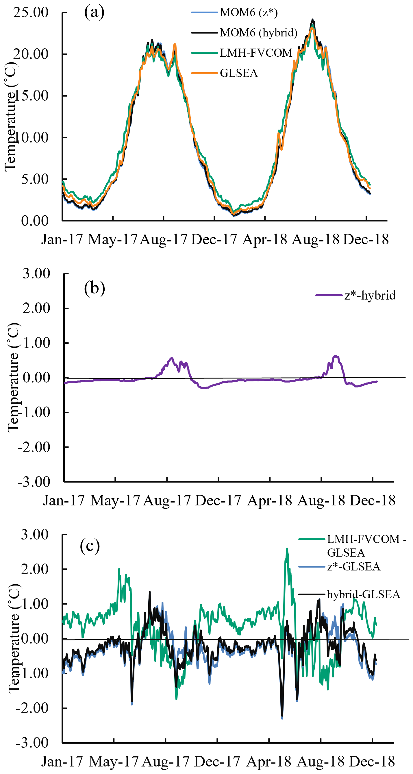
Figure 2 (a) Time series (2017–2018) of simulated daily average lake surface temperature (LST; °C) by MOM6-SIS2-LMH vertical coordinate system (VCSs) (z^∗ and hybrid), LMH-FVCOM and satellite estimates (Great Lakes Surface Environmental Analysis; GLSEA). (b) The difference in LST between z^∗ and hybrid VCSs during 2017–2018. (c) The difference in LST timeseries between z^∗, hybrid, LMH-FVCOM, and GLSEA. Model results for z^∗, hybrid, LMH-FVCOM, and GLSEA are shown in blue, black, green, and orange, respectively. In panel (a), the two MOM6–SIS2 configurations largely overlap, with the MOM6–SIS2, z^∗ results often overlain by the MOM6-SSI2 hybrid line.

Table 2 Model validation metrics for daily averaged lake surface temperature (LST; 2017–2018) for MOM6-SIS2-LMH vertical coordinate systems (VCSs; z^∗ and hybrid) and LMH-FVCOM. Metrics were derived by comparison of simulated LST to satellite estimates (Great Lakes Surface Environmental Analysis; GLSEA) LST.

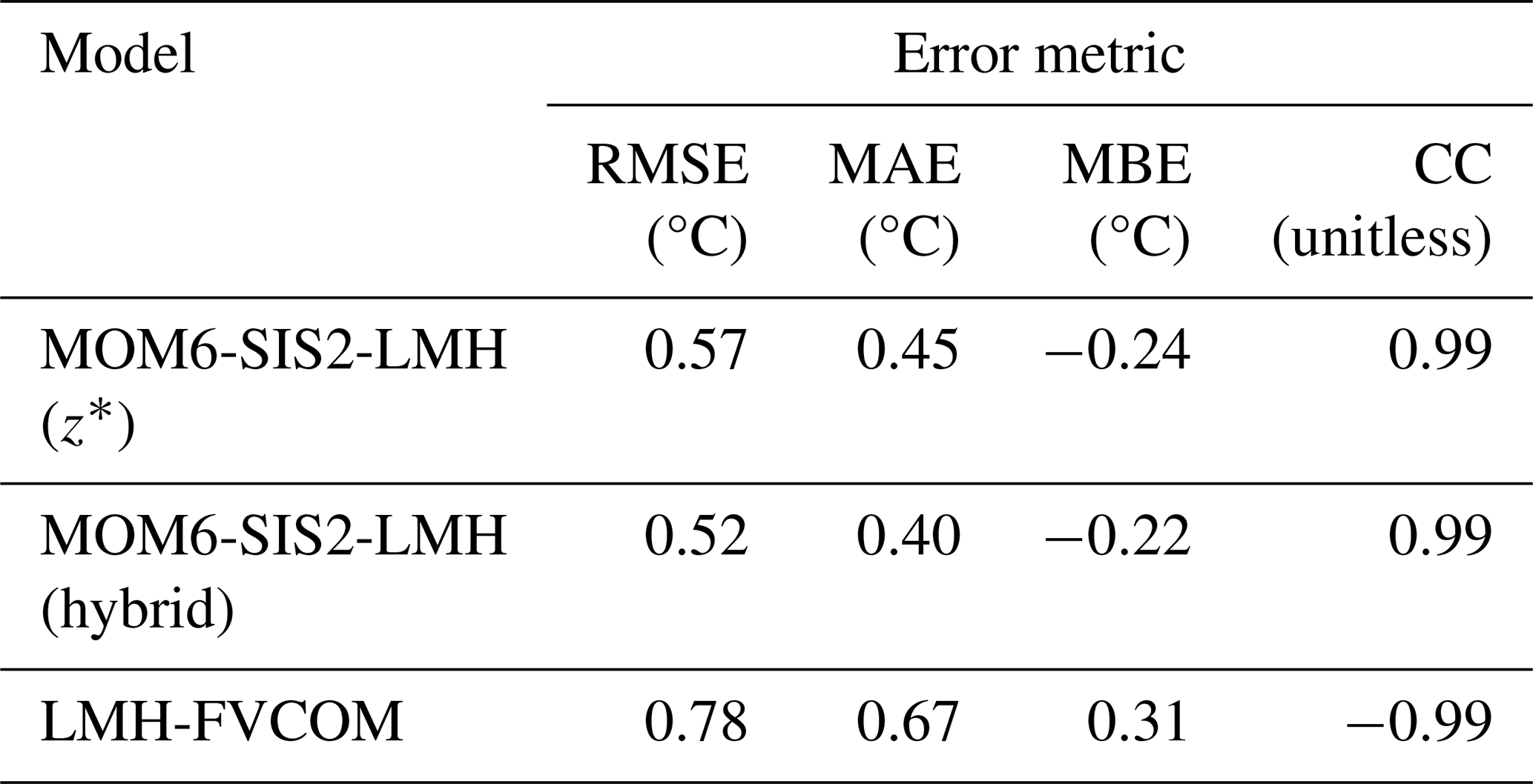
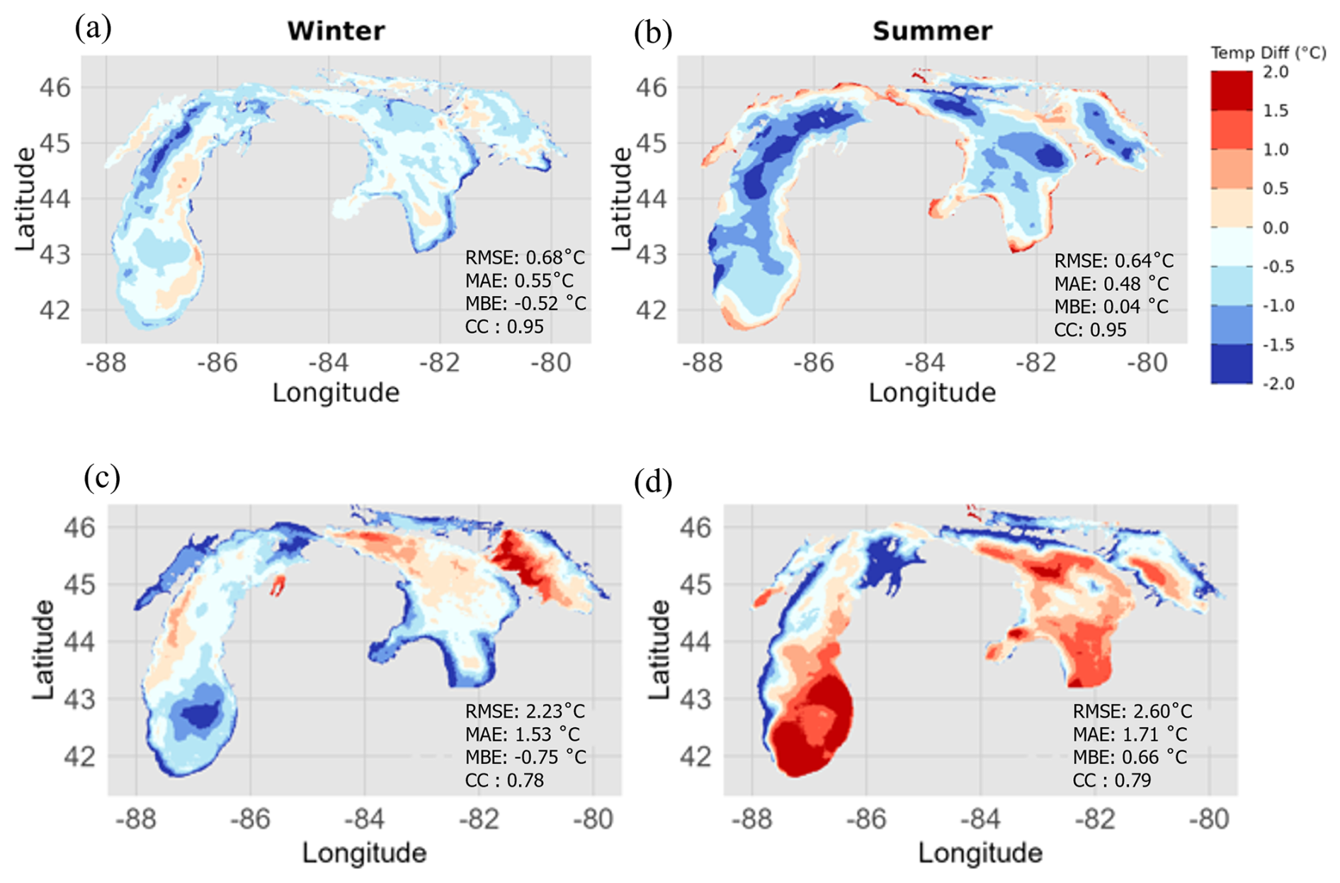
Figure 3 Difference between MOM6-SIS2-LMH's (hybrid VCS) seasonally averaged lake surface temperatures and satellite estimates from the Great Lakes Surface Environmental Analysis (GLSEA) for (a) winter and (b) summer in 2017. Difference between LMH-FVCOM's seasonally averaged lake surface temperatures and satellite estimates from the GLSEA for (c) winter and (d) summer in 2017. The error metrics, Root Mean Square Error (RMSE), Mean Absolute Error (MAE), Mean Bias Error (MBE), and Pearson Correlation Coefficient (CC) between simulations and observations are shown in the bottom right corner of the plots.

Seasonally averaged LST differences between the simulations and observations are shown for the year 2017 (Figs. 3 and S4 in the Supplement). When winter and summer LST differences were compared spatially for MOM6-SIS2-LMH (hybrid VCS) (Fig. 3a and b) and LMH-FVCOM (Fig. 3c and d), notable differences were apparent in these two seasons for both models. In MOM6-SIS2-LMH, widespread cool bias was observed in winter (Fig. 3a), while summer differences were more spatially variable, with warm bias mostly concentrated near the shorelines and a cool bias in the offshore (Fig. 3b). In contrast, LMH-FVCOM exhibited a warm bias during the winter (Fig. 3c) and greater variability in summer (Fig. 3d) with notable regions of cool bias along the northern coastline and warm bias in the southern regions. MOM6-SIS2-LMH hybrid VCS exhibited better skill than LMH-FVCOM for all seasons (Figs. 3 and S4). Comparison of MOM6-SIS2 z^∗ VCS and LMH-FVCOM for all seasons are shown in Fig. S5 in the Supplement.

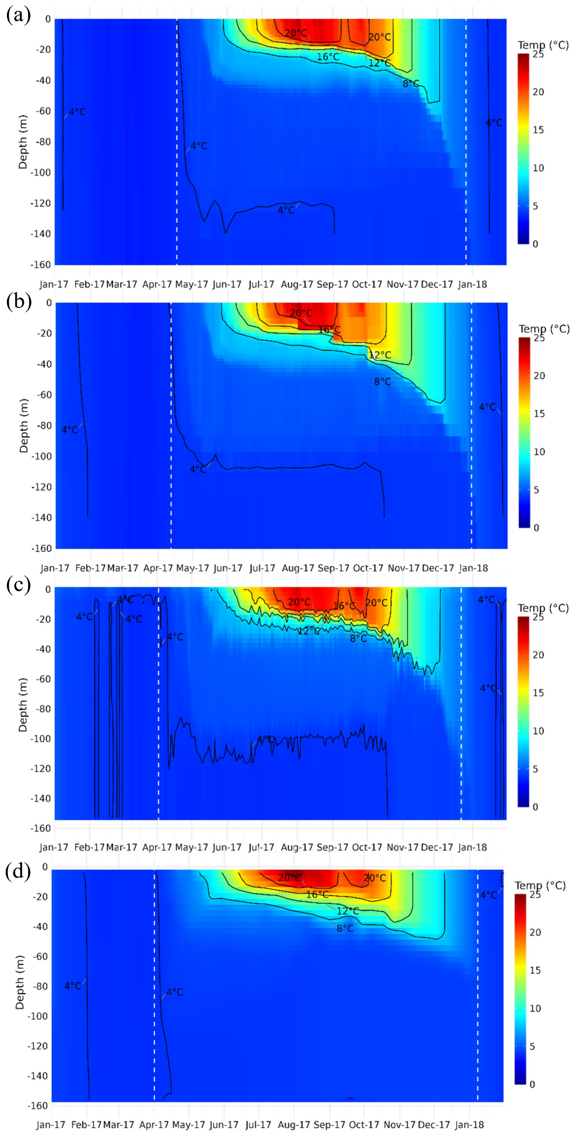
Figure 4 Vertical thermal profile (January 2017–January 2018) at a thermistor string station located in southern Lake Michigan (location shown in Fig. 1). Temperature profiles simulated by the MOM6-SIS2-LMH VCSs at daily resolution for (a) z^∗, (b) hybrid, (c) the observed temperature profile at hourly resolution, and (d) the simulated temperature profile at daily resolution simulated by the Lake Michigan-Huron – Finite Volume Community Ocean Model (LMH-FVCOM).

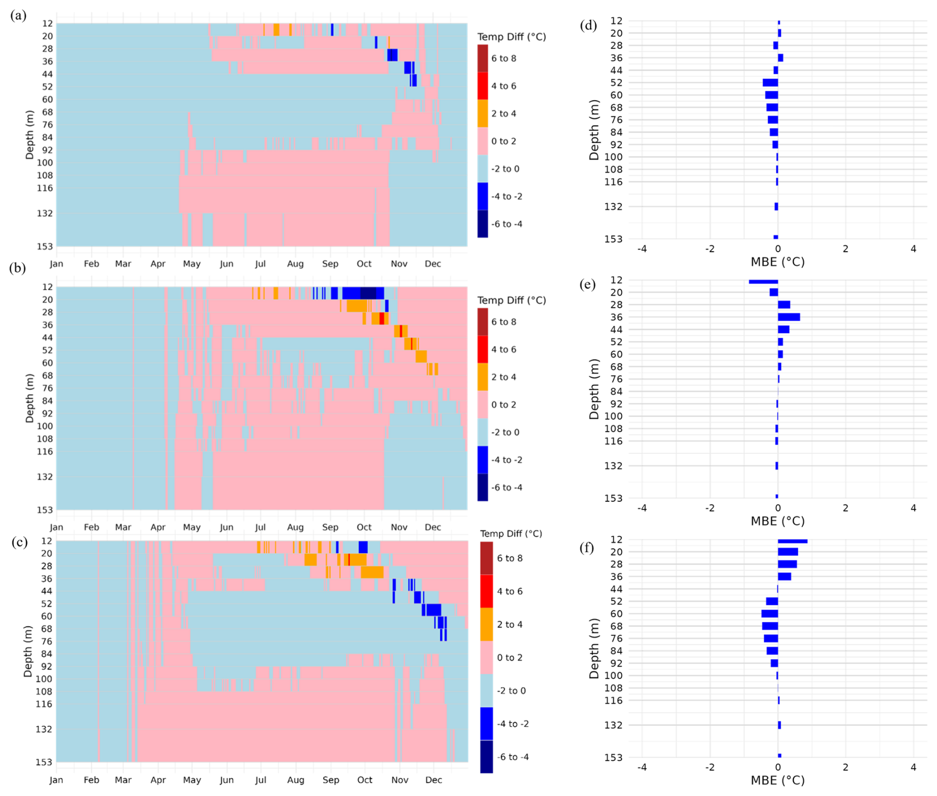
Figure 5 Difference between simulated and observed vertical thermal profiles at a thermistor string station located in southern Lake Michigan for 2017, simulated by MOM6-SIS2-LMH (a) z^∗, (b) hybrid VCSs, and (c) LMH-FVCOM. The Mean Bias Error (MBE) at corresponding depths for MOM6-SIS2-LMH z^∗, hybrid, and LMH-FVCOM are shown in (d), (e), and (f), respectively.

Table 3 Summer stratification onset and fall overturn dates, stratification duration, average depth of the 12 and 8 °C isotherms, average distance between isotherms for observations, MOM6-SIS2-LMH VCSs and LMH-FVCOM at a thermistor string station located in southern Lake Michigan in 2017. The average depth and the distance between isotherms were calculated over the period June–August 2017.

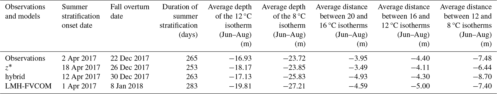
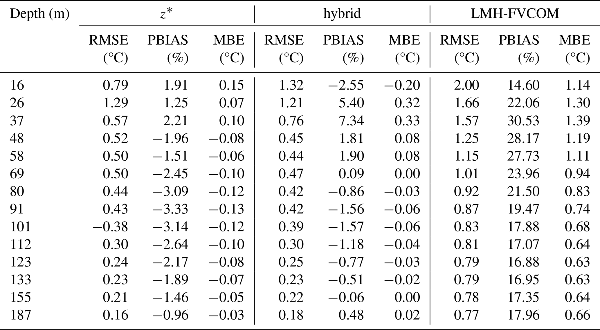
Table 4 Skill assessment of the MOM6-SIS2-LMH VCSs and LMH-FVCOM, in simulating sub-surface temperatures recorded at a thermistor sting station in southern Lake Michigan for the year 2017.

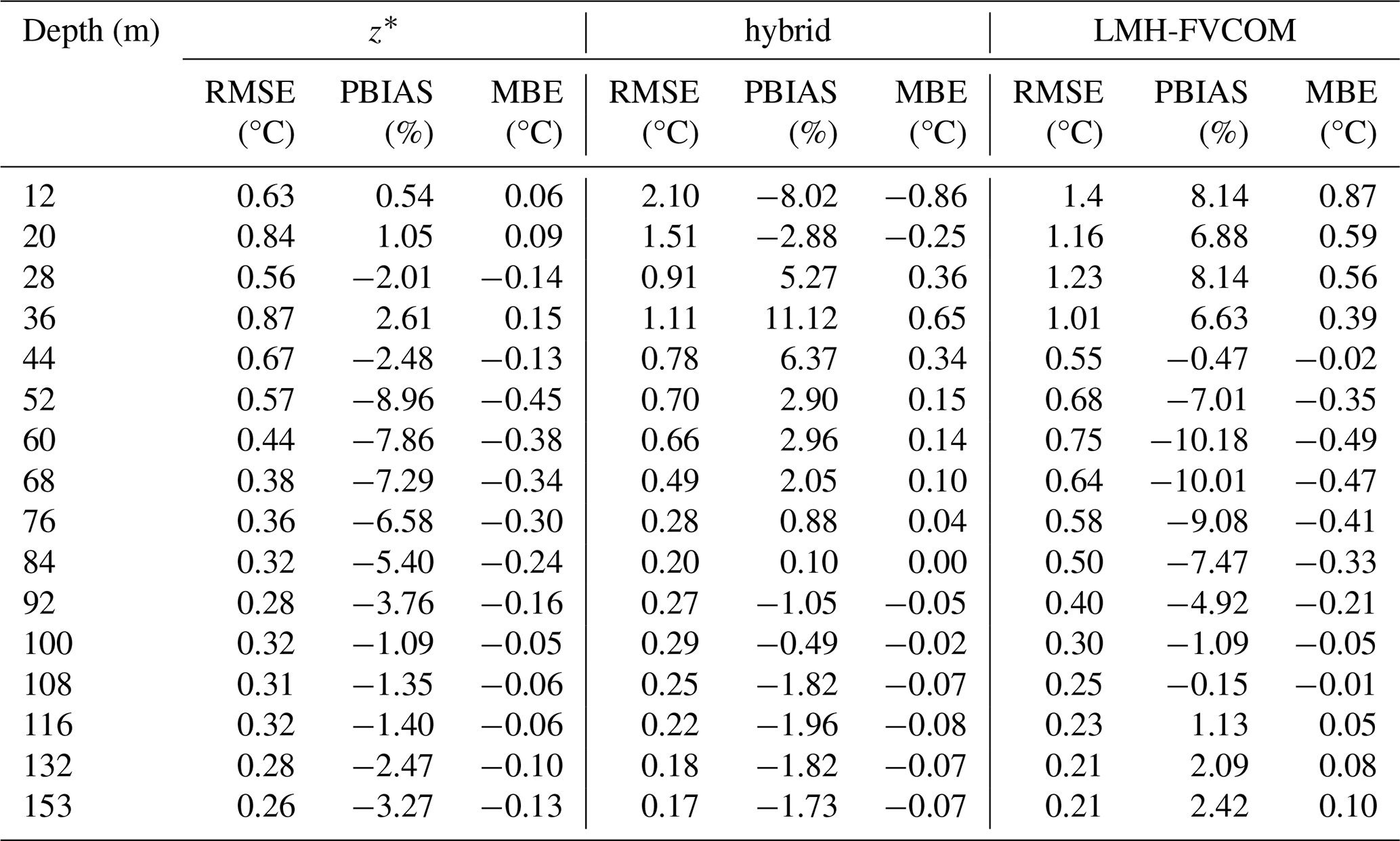
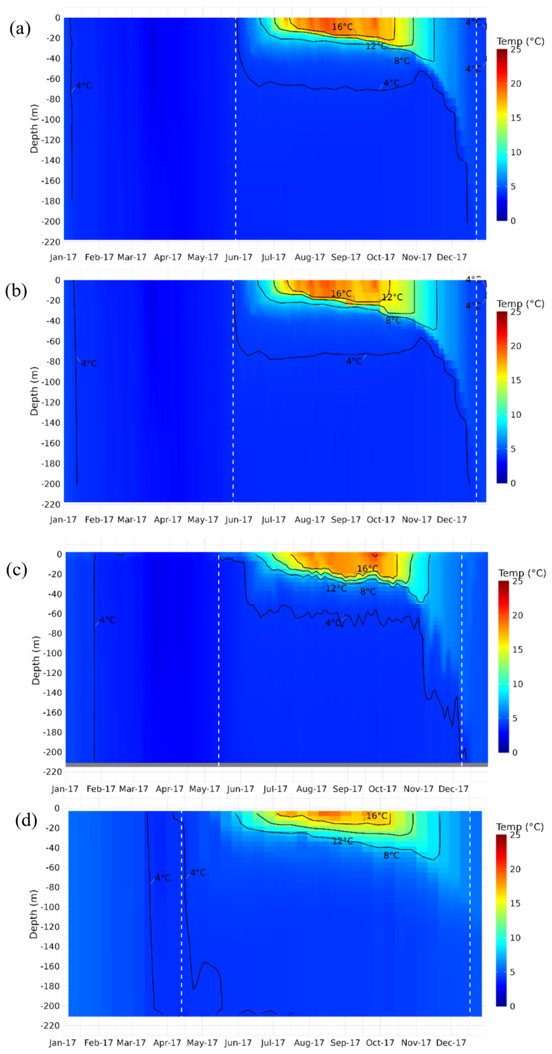
Figure 6 Vertical thermal profile across 2017 at a thermistor string station located in central Lake Huron (location shown in Fig. 1). Temperature profiles simulated by the MOM6-SIS2-LMH VCSs at daily resolution for (a) z^∗, (b) hybrid, (c) the observed temperature profile at hourly resolution, and (d) the simulated temperature profile at daily resolution simulated by the Lake Michigan-Huron – Finite Volume Community Ocean Model (LMH-FVCOM).

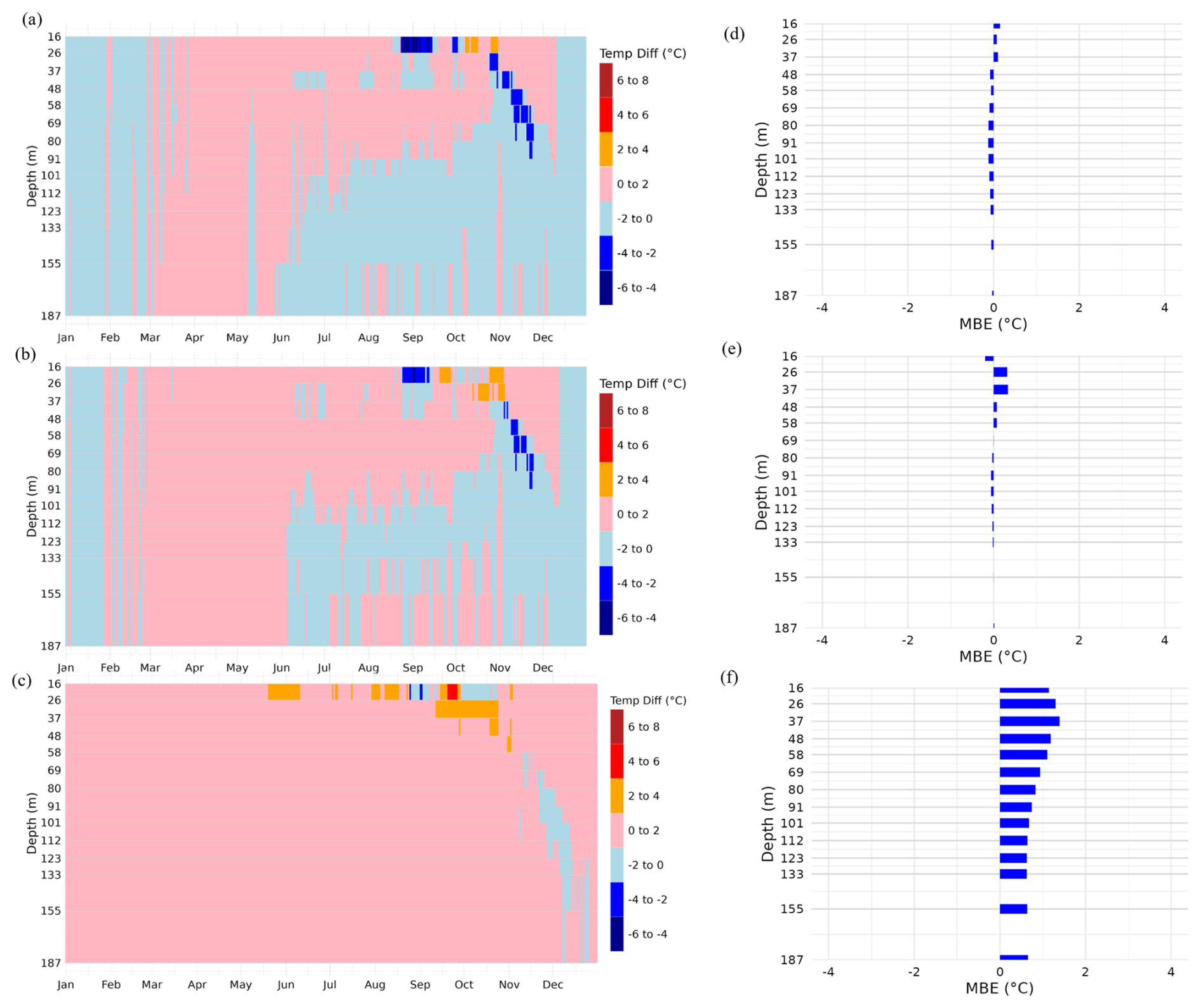
Figure 7 Difference between simulated and observed vertical thermal profiles at a thermistor string station located in central Lake Michigan for 2017, simulated by MOM6-SIS2-LMH VCSs (a) z^∗, (b) hybrid, and (c) LMH-FVCOM. The Mean Bias Error (MBE) at corresponding depths for MOM6-SIS2-LMH z^∗, hybrid, and LMH-FVCOM are shown in (d), (e), and (f), respectively.

Table 5 Summer stratification onset and fall overturn dates, stratification duration, average depth of the 12 and 8 °C isotherms, average distance between isotherms for observations, MOM6-SIS2-LMH VCSs and LMH-FVCOM at a thermistor string station located in central Lake Huron in 2017. The average depth and the distance between isotherms were calculated over the period June–August 2017.

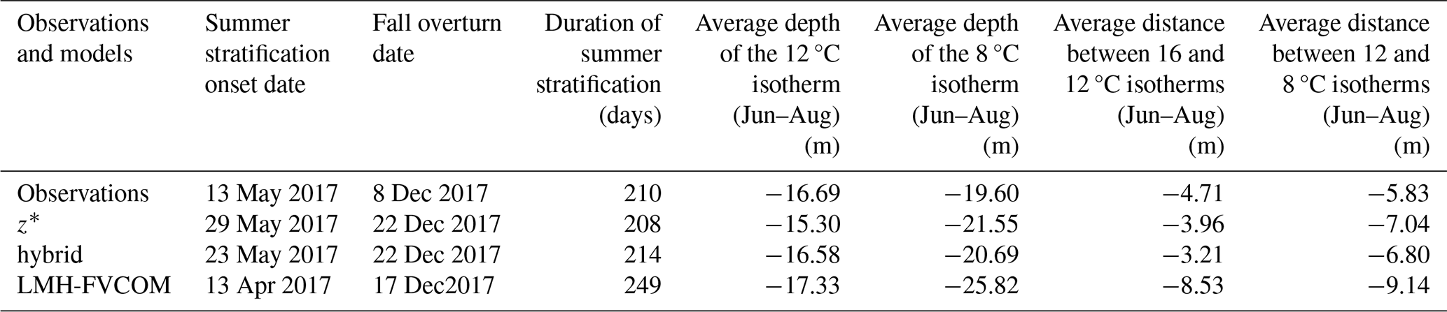
Table 6 Skill assessment of the MOM6-SIS2-LMH VCSs and LMH-FVCOM, in simulating sub-surface temperatures recorded at a thermistor string station located in central Lake Huron for the year 2017.

3.2 Vertical thermal structure

Overall, both MOM6-SIS2-LMH VCSs capture the onset of summer stratification, fall overturn date, duration of stratification, and the gradual deepening of the thermocline (approximated as the area between the 12 and 8 °C isotherms) reasonably well in comparison to observations and LMH-FVCOM at southern Lake Michigan (Figs. 4 and 5; Tables 3 and 4) and at central Lake Huron thermistor string locations (Figs. 6 and 7; Tables 5 and 6). Compared to LMH-FVCOM, MOM6-SIS2-LMH VCSs reproduced a more realistic thermocline depth and vertical temperature gradient, suggesting improved representation of vertical mixing and entrainment processes.

Specifically, MOM6-SIS2-LMH VCSs demonstrated more accurate entrainment at the 4 °C isotherm at both thermistor string locations, maintaining the integrity of deep cold water while minimizing artificial upward mixing, which helps preserve a stable and well-defined hypolimnion throughout the stratified season (Figs. 4 and 6). The average distance between the isotherms for the period June–August 2017 at southern Lake Michigan and central Lake Huron locations, respectively, are shown in Table 3 and 5. At southern Lake Michigan, MOM6-SIS2-LMH VCSs exhibited delayed onset of summer stratification and a later fall overturn date, slightly underestimating the stratification duration and simulating a deeper thermocline compared to observations (Fig. 4a–c; Table 3).

However, when comparing between the MOM6-SIS2-LMH configurations with different VCSs, notable differences are observed in the stratification dates and thermocline depths. The MOM6-SIS2-LMH hybrid VCS simulates an earlier onset of summer stratification and later fall overturn date, resulting in a longer stratification period than the z^∗ VCS and close to observations (Table 3). Additionally, the hybrid configuration sustains a deeper and more stable thermocline, as evidenced by a distinct, continuous cold-water pool marked by the 4 °C isotherm (Fig. 4) and a reduced bias error in deep waters (MBE < ± 0.5 °C, below 76 m; Fig. 5 and Table 4).

At central Lake Huron, MOM6-SIS2-LMH VCSs closely matched observed stratification onset, fall overturn dates, and duration, while LMH-FVCOM significantly overestimated stratification period and depth of the cold-water layer (Fig. 6, Table 5). Both MOM6-SIS2-LMH VCSs produced realistic thermocline and hypolimnion depths and maintained a stable 4 °C isotherm, whereas LMH-FVCOM over-deepened the cold-water pool. Skill metrics (Fig. 7 and Table 6) confirm MOM6-SIS2-LMH VCSs improved performance throughout the water column, especially below 58 m (MBE < ± 0.2 °C; Table 6), highlighting its improved performance in simulating lake thermal structure at this location. MOM6-SIS2-LMH z^∗ and hybrid VCSs both simulated the thermal structure with similar skill. Both VCSs closely match the stratification dates and duration (Table 5), and the depths of the 4 °C isotherms differ only slightly between the two. Their temperature error statistics are nearly identical across the water column, with low RMSE values (typically  0.5 °C below 58 m) and minimal bias at all depths.

3.3 Inertial oscillations

The depth of the 17 °C isotherm, a proxy for the thermocline depth, was vertically interpolated for models (MOM6-SIS2-LMH (hybrid VCS), LMH-FVCOM) and observations. A spectral analysis was conducted for simulated and observed isotherm depths to examine inertial oscillations in the lake (Fig. 8), which are expected to dominate thermocline variability during the stratified period. Spectral density plots for MOM6-SIS2-LMH and LMH-FVCOM both agree well with observations in the inertial and sub inertial range (f < 0.08 h⁻¹), with spectral peaks that match the expected 17.7 h local inertial period. MOM6-SIS2-LMH and LMH-FVCOM, however, are less energetic than observations at all frequencies, highlighting consistently lower amplitudes for simulated thermocline oscillations. Simulated and observed spectral densities also deviate significantly at high frequencies, where observations exhibit flat-lined behaviour that is indicative of instrument noise floors.

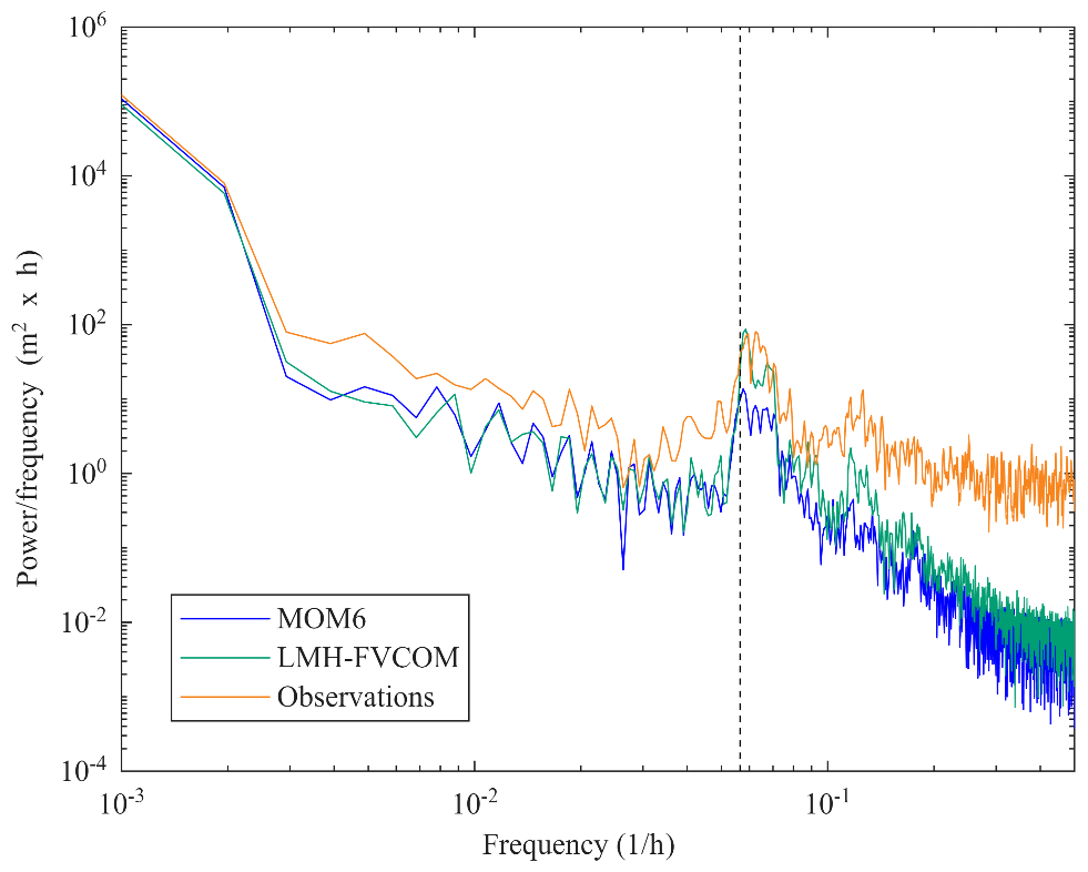
Figure 8 Spectral analysis of the 17 °C isotherm depth time series. The plot shows power density (m²) as a function of period (days) on log-log scales for observations (orange) and simulations (MOM6-SIS2-LMH (hybrid-VCS): blue; LMH-FVCOM: green) at southern Lake Michigan thermistor string station during the summer of 2017 (July–September). The dashed vertical line marks the 17.7 h reference period.

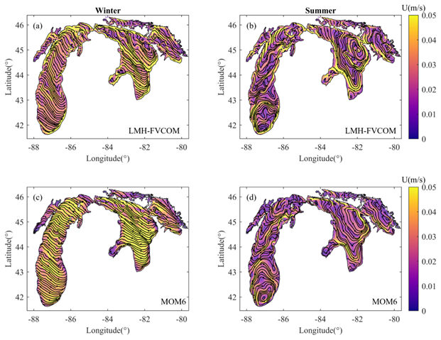
Figure 9 Seasonally averaged winter (a, c) and summer (b, d) current patterns for LMH-FVCOM (a, b) and MOM6-SIS2-LMH (c, d) during 2017.

3.4 Seasonal mean circulation and nearshore processes

Both z^∗ and hybrid VCSs show comparable skill in simulating surface temperature variability (Fig. 2), therefore, the hybrid VCS is presented here for clarity and brevity, as it adequately represents MOM6-SIS2 behavior for the processes examined. Seasonally averaged winter and summer circulation simulated by MOM6-SIS2-LMH (hybrid VCS) and LMH-FVCOM for the year 2017 are shown in Fig. 9. In winter, the MOM6-SIS2-LMH (hybrid VCS) simulation shows a cyclonic gyre in Lakes Michigan and Huron, where surface currents are primarily driven by wind shear. In summer for Lake Michigan, MOM6-SIS2-LMH (hybrid VCS) shows an anticyclonic gyre in the southern region and a cyclonic gyre in the northern region. In Lake Huron, a basin-wide cyclonic gyre is simulated by MOM6-SIS2-LMH (hybrid VCS). Comparing MOM6-SIS2-LMH (hybrid VCS) with LMH-FVCOM indicates that both models show similar large-scale, basin-wide circulation patterns with similar speed ranges (up to 0.05 m s⁻¹) and general seasonal shifts in winter and summer. However, LMH-FVCOM performs better by exhibiting higher velocities in nearshore areas and around complex bathymetric features (Straits of Mackinac).

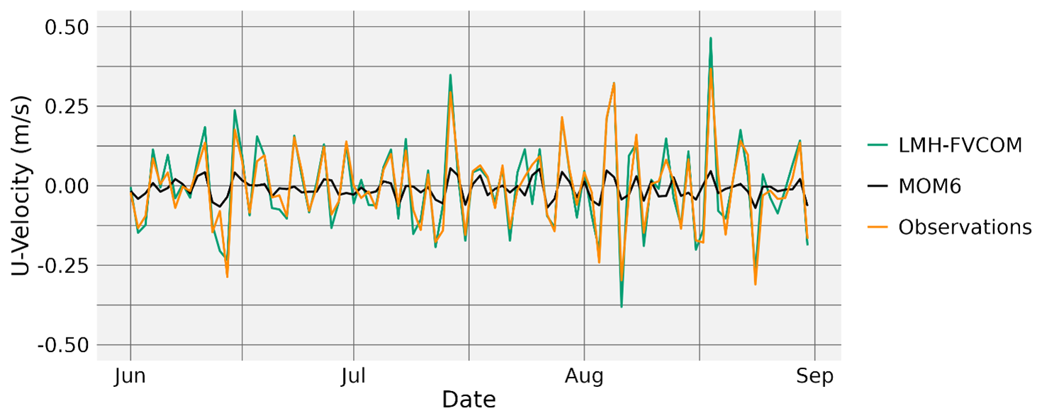
Figure 10 Depth-averaged u-velocities from observations (orange), MOM6-SIS2-LMH (black), and LMH-FVCOM (green) at a UGLOS station in the Straits of Mackinac during June to September 2017. Location of this UGLOS station is shown in Fig. 1.

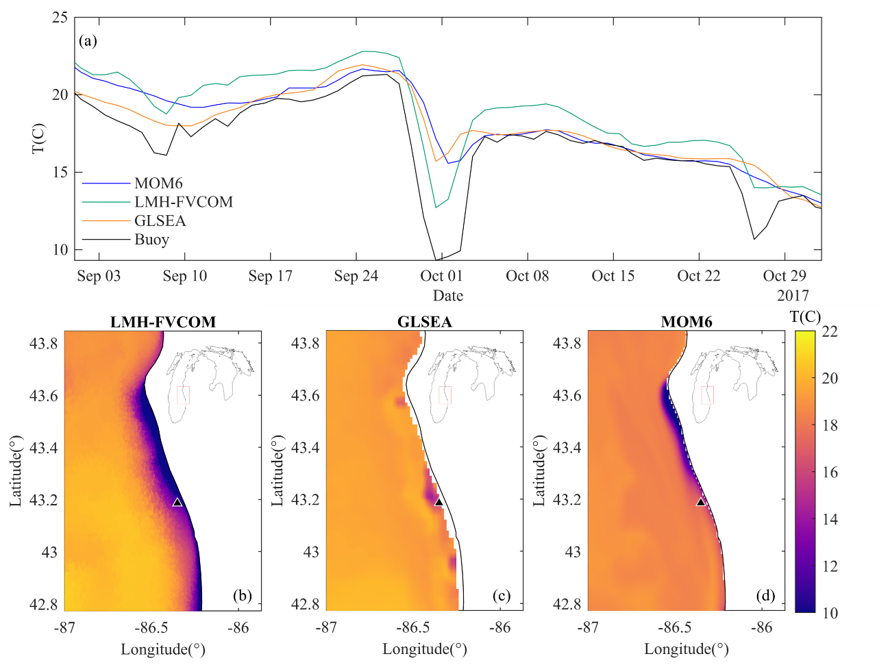
Figure 11 Lake surface temperatures as observed and simulated during a coastal upwelling event on the eastern coast of Lake Michigan between 1 September and 30 October 2017. Time series of simulations (blue: MOM6-SIS2-LMH (hybrid VCS); green: LMH-FVCOM) and observations (orange: GLSEA; black: buoy) collocated with a meteorological buoy (black triangle) are shown in (a). Spatial maps of observed (c: GLSEA) and simulated (b: LMH-FVCOM; d: MOM6-SIS2-LMH) surface temperatures on 1 October 2017, are included for reference.

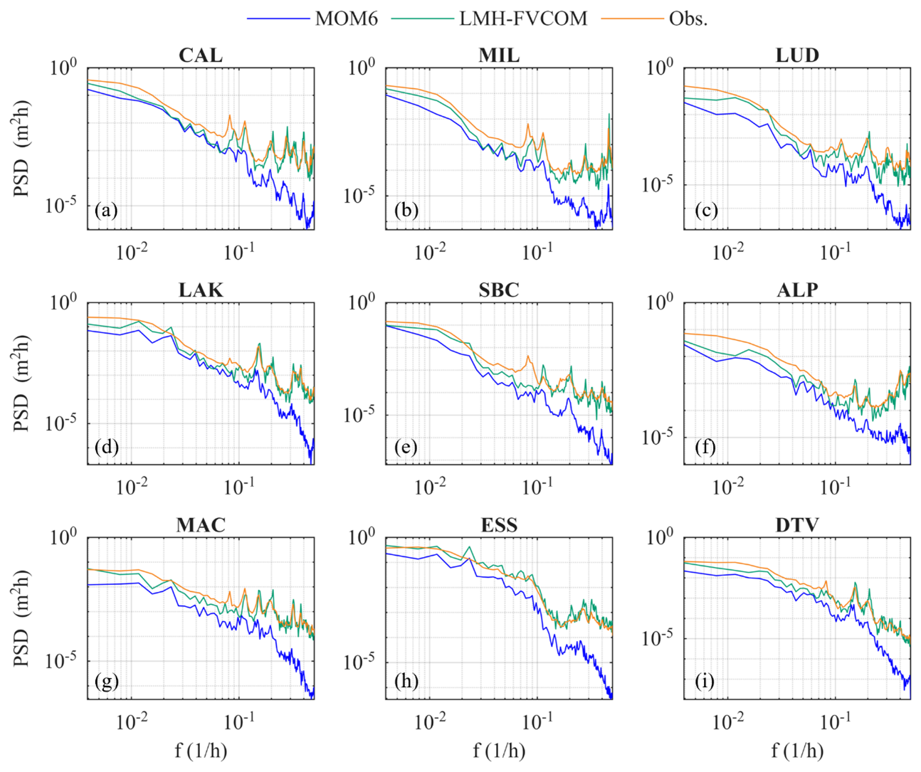
Figure 12 Power spectral density plots for water level fluctuations as simulated (MOM6-SIS2-LMH (hybrid VCS): blue; LMH-FVCOM: green) and observed (orange) between 1 July and 31 December 2017. Location of water level stations are shown in Fig. 1.

Performance of MOM6-SIS2-LMH (hybrid VCS) in capturing the bi-directional flow at Straits of Mackinac and simulating the nearshore processes are shown in Figs. 10–12. MOM6-SIS2-LMH successfully reproduces the observed bi-directional flow patterns at Straits of Mackinac (UGLOS station shown in Fig. 1), capturing both the timing and directionality of the velocity fluctuations despite only having 1 km horizontal resolution (Fig. 10). However, it underestimates the magnitude of velocities throughout the time-series. This suggests that, although MOM6-SIS2-LMH captures the qualitative dynamics of the bi-directional flow patterns, it does not fully resolve the energetic variability as seen in LMH-FVCOM. This underestimation arises primarily from the coarser horizontal resolution in MOM6-SIS2-LMH, which limits the model's ability to represent small-scale turbulent and nearshore processes that contribute to energetic variability. In contrast, LMH-FVCOM, with its finer unstructured grid, better resolves these features and captures higher-frequency velocity fluctuations.

To further assess MOM6-SIS2-LMH's performance in the nearshore, model simulations of surface temperature were compared to nearshore buoy observations and GLSEA satellite estimates during a coastal upwelling (Fig. 11). While both models (MOM6-SIS2-LMH (hybrid VCS) and LMH-FVCOM) and GLSEA captured the timing of the buoy-observed temperature decline in late September, all three, but particularly MOM6-SIS2-LMH and GLSEA, underestimated the amplitude of the rapid surface cooling during the upwelling relative to the buoy data. Spatial maps indicate that MOM6-SIS2-LMH and GLSEA produces smoother temperature gradients along the nearshore region, whereas LMH-FVCOM reveal a much sharper thermal fronts and greater nearshore variability (Fig. 11b–d). Overall, MOM6-SIS2-LMH reproduces large-scale temporal and spatial temperature trends, but underestimates extremes and nearshore variability relative to LMH-FVCOM.

Water level fluctuations in Lake Michigan and Lake Huron were analyzed using Power Spectral Density (PSD) techniques to investigate how well lake seiches are captured by LMH-FVCOM and MOM6-SIS2-LMH (Fig. 12). While simulated mean water levels are not expected to match observations, because the models do not include external freshwater mass fluxes (river inputs, precipitation and evaporation), barotropic surface oscillations should still be well captured by both models. Although both models perform well in capturing the peak frequencies of water level fluctuations across the lake, LMH-FVCOM demonstrates much closer agreement with observations, particularly at higher frequencies, where MOM6-SIS2-LMH tends to under-predict peak energies by several orders of magnitude. Because PSD represent the distribution of water-level variance, the energy deficits imply substantially reduced variance at high frequencies, corresponding to high-frequency seiche amplitudes in MOM6-SIS2-LMH that are approximately an order of magnitude smaller than observed. These underpredictions are indicative of low biases in simulated nearshore seiche amplitudes, likely resulting from the coarse resolution (i.e. 1 km) coastal grid used in our MOM6-SIS2-LMH configuration (discussed in Sect. 4.3).

3.5 Ice concentration

Both MOM6-SIS2-LMH VCSs and LMH-FVCOM closely capture the timing and spatial extent of observed ice concentration, USNIC (Fig. 13). During the 2017 winter, however, both MOM6-SIS2-LMH VCSs overestimated ice concentration compared to USNIC observations and LMH-FVCOM. For example, both MOM6-SIS2-LMH VCSs simulated peak ice concentrations of ∼ 35 %–40 % in the winter of 2017, while USNIC reports a peak closer to 25 % (Fig. 13a). The simulated ice concentration remains elevated for a longer period than the observed values and LMH-FVCOM, reflecting a RMSE of close to 5 % during much of the winter 2017 season. During the winter of 2018, MOM6-SIS2-LMH VCSs performed well, with simulated and observed peaks within 2 %–5 % (both reaching ∼ 63 %–65 %). During these events, MOM6-SIS2-LMH VCSs successfully capture the duration of the ice season indicated in observations.

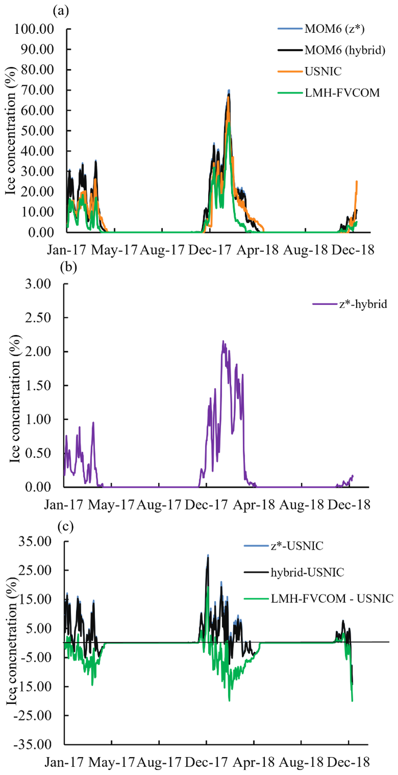
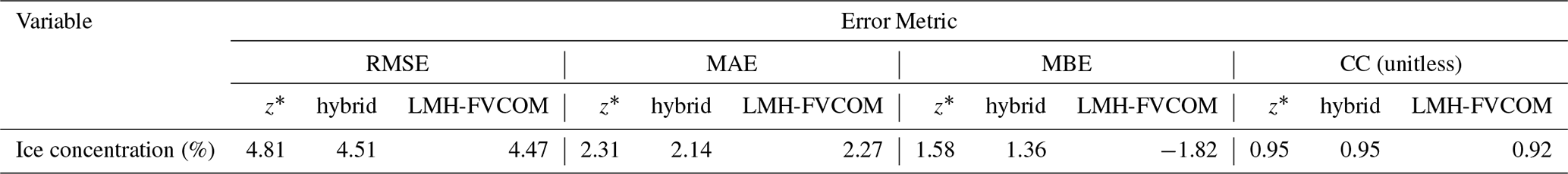
Figure 13 (a) Time series (2017–2018) of daily average lake ice concentration (%) in Lake Michigan-Huron simulated by MOM6-SIS2-LMH VCSs (z^∗ and hybrid), LMH-FVCOM, and United States National Ice Center (USNIC). (b) Difference in ice concentration (%) between z^∗ and hybrid vertical coordinate systems (VCSs) during 2017–2018. (c) Difference in ice concentration (%) time series between z^∗, hybrid, LMH-FVCOM, and USNIC. Model results for z^∗, hybrid, LMH-FVCOM, and USNIC are shown in blue, black, green, and orange, respectively.

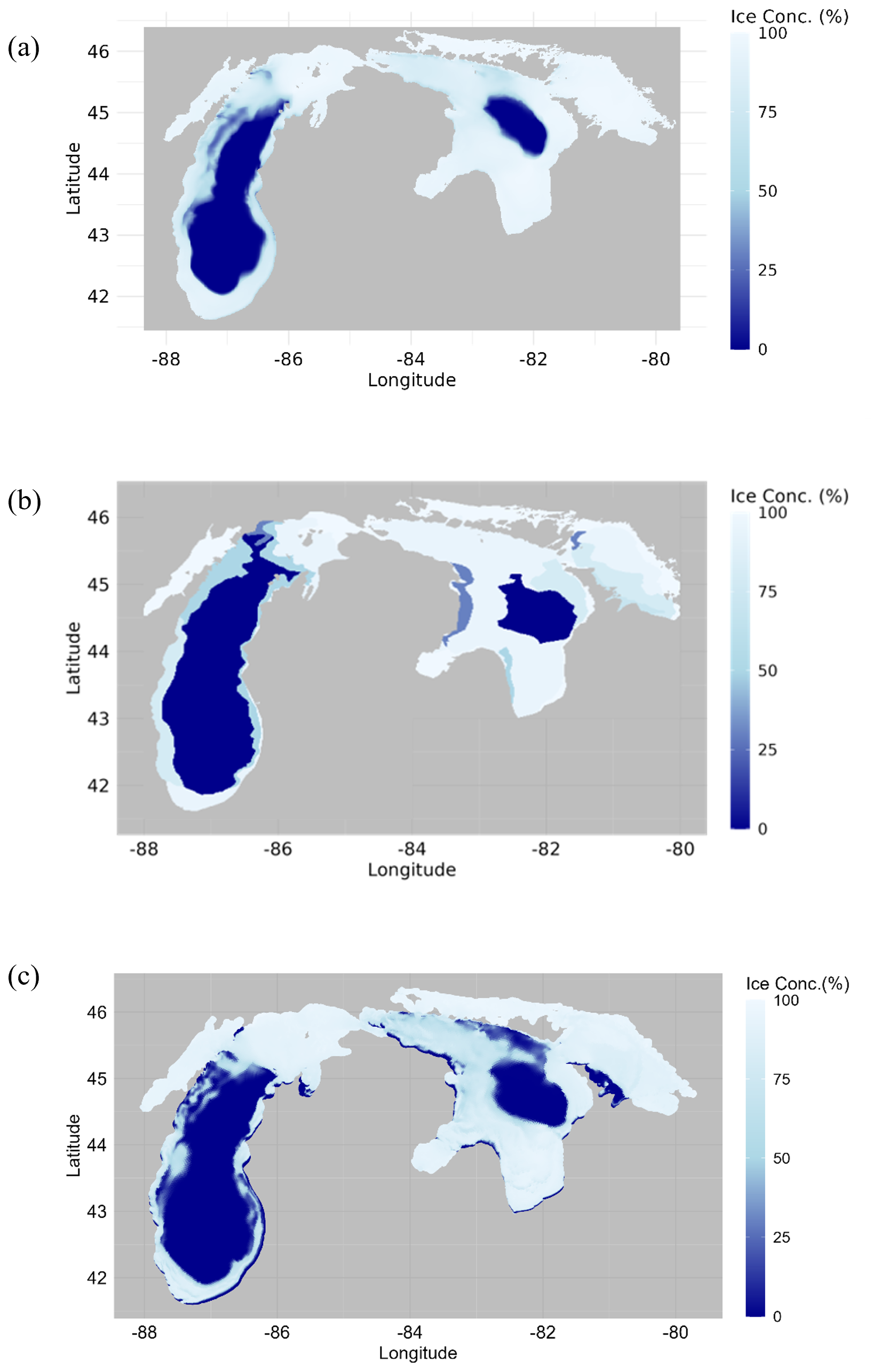
Figure 14 Comparison of ice concentration (%) as simulated by (a) MOM6-SIS2-LMH (hybrid- vertical coordinate system (VCS)), (b) observations (i.e. United States National Ice Center, USNIC), and (c) LMH-FVCOM on the day of observed maximum ice cover during the simulation period: 13 February 2018.

Differences in simulated ice concentration between z^∗ and hybrid VCSs were below 2.5 % for most of the period, even during ice maxima (Fig. 13b). During the winter of 2017, both z^∗ and hybrid VCSs overestimated ice concentrations by more than 10 %, which was greater than the absolute error of LMH-FVCOM for that period. Spatial maps of ice concentration and ice thickness during maximum ice event in 2018 (February 13) indicate that MOM6-SIS2-LMH reasonably simulates the spatial patterning of ice concentration in comparison to USNIC and LMH-FVCOM (Figs. 14 and S6 in the Supplement). Additionally, MOM6-SIS2-LMH VCSs generally overestimated ice observations in both winters where LMH-FVCOM tended to underestimate, and MOM6-SIS2-LMH captured the rate of ice melt in April 2018 better than LMH-FVCOM.

4 Discussion

4.1 Evaluating the performance of MOM6-SIS2 in large freshwater lakes

In this study, we have shown that MOM6-SIS2 is a viable hydrodynamic modeling framework for large freshwater lakes. MOM6-SIS2-LMH simulations were able to reliably reproduce spatial and seasonal patterns in circulation, surface temperature, ice cover, and vertical thermal structure. LST and ice cover simulations were characterized by seasonal stratification cycles (Figs. 2 and 13), with an inversely stratified, ice-covered winter (January–March) and a stably stratified summer (May–September) delineated by isothermal turnover periods in the spring (∼ April) and fall (∼ October). The timing and spatial variability of simulated stratification cycles agreed well with previous studies (Anderson et al., 2021; Cannon and Troy, 2018), highlighting the typical progression of warming and/or cooling from nearshore to offshore waters (i.e., thermal bar dynamics). MOM6-SIS2-LMH simulated seasonal circulation patterns (Fig. 9) are consistent with previous observational Beletsky et al. (1999), and modeling studies, Beletsky et al. (2006) and Zhang et al. (2025), highlighting persistent inertial rotational gyres in the stratified summer and wind-driven coastal currents during the energetic winter. Importantly, the model proved to be suitable for use in Great Lakes modeling applications by capturing the system's key physical processes, including near-inertial Poincare waves (Fig. 8), which dominate offshore currents and thermocline fluctuations during the stratified summer (Choi et al., 2015), and basin-scale standing waves, or seiches, which drive coastal currents and water-level fluctuations throughout the year (Anderson and Schwab, 2013, 2017).

MOM6-SIS2-LMH performed as well or better than LMH-FVCOM at the lake wide scale, and, in fact, offered significant improvements in both surface temperature (RMSE: MOM6-SIS2-LMH (hybrid VCS) – 0.52 °C, LMH-FVCOM-0.78 °C), vertical thermal structure (MOM6-SIS2-LMH VCSs demonstrated more accurate entrainment at the 4 °C isotherm at both thermistor string locations), and ice concentration (RMSE: MOM6-SIS2-LMH (hybrid VCS) – 4.51 %, LMH-FVCOM – 4.47 %). Importantly, both models produced similar surface circulation patterns, and each was able to reproduce observed inertial thermocline oscillations. However, MOM6-SIS2 struggled to accurately simulate coastal processes that were well captured by LMH-FVCOM, including coastal upwellings, persistently strong coastal surface currents, and inter basin transport through the Straits of Mackinac. These shortcomings are discussed in Sect. 4.3.

Table 7 Model validation metrics for daily averaged lake wide ice concentration (%) across 2017–2018 using two different vertical coordinate configurations (VCSs) of MOM6-SIS2-LMH and LMH-FVCOM.

Performance metrics for MOM6-SIS2-LMH simulations (LST and ice-cover) matched or exceeded those of other models used in the region. Although direct model-to-model comparisons are complicated by variable atmospheric forcing choices and simulation periods, published performance metrics still provide a valuable baseline for comparison. For example, Cannon et al. (2023, 2024), described Lake Michigan-Huron simulations (model: FVCOM v3.1.6; period: 1979–2021; atmospheric forcing: NARR) with lake wide annual LST (ice cover) RMSE in excess of 1 °C (7 %), nearly twice as high as those reported in the current study (LST: 0.52 °C; ice concentration : 4.5 % – Tables 2 and 7). MOM6-SIS2-LMH also compared favourably with two-way coupled lake-atmosphere models, including the Great Lakes Atmosphere Regional Model, GLARM (Xue et al., 2017), which reported model RMSEs of 0.65–0.79 °C (surface temperature) and 1.75 %–2.49 % (ice cover) for an ERA-Interim forced simulation between 2003–2014.

We have shown that MOM6-SIS2-LMH is especially adept at resolving deepwater thermal structure in weakly stratified lakes. Comparison with thermistor string observations indicates that MOM6-SIS2-LMH not only reliably reproduced temperature profiles throughout the water column (MBE < ± 0.5 °C below 50 m depth, Table 4 and 6) but also outperformed LMH-FVCOM in representing deeper thermocline layers (Figs. 4 and 6). In particular, simulations align well with observed thermocline development and turnover dates in offshore waters, predicting the spring and fall turnovers within two weeks of observations. Perhaps most importantly, the model is able to sustain very weak deep-water stratification, including representation of the 4 °C isotherm, which is notably absent from the LMH-FVCOM simulations. LMH-FVCOM is not alone in this regard; overly-diffuse thermal structure – particularly around the thermocline, has been a long-standing issue for historical and contemporary Great Lakes hydrodynamics models (e.g. Bai et al., 2013; Beletsky and Schwab, 2001; Rowe et al., 2019; Xue et al., 2017). Although there has been some success in sharpening the thermocline through integration scheme modifications and wind-wave mixing parameterizations (e.g. Bai et al., 2013), over-diffusion remains an ongoing issue for the Great Lakes modeling community. The flexibility and stability of MOM6-SIS2 make it an attractive solution for this problem.

In this study, calibration tests (not shown) suggested that simulated thermal structure was most sensitive to the mixing characteristics; in particular, background diapycnal diffusivity (KD). By decreasing KD to molecular values (KD = 1 × 10⁻⁷ m² s⁻¹), we were able to reduce spurious background diffusion and sharpen the thermocline, even in the absence of a hybrid VCS (discussed in Sect. 4.2). Importantly, these changes are consistent with observations of mixing in the lake. Without energetic tides, currents in the Great Lakes are relatively weak, with maximum near-surface velocities of just 0.25 m s⁻¹ reported at a 55 m deep site in Lake Michigan (Cannon and Troy, 2018). Previous studies have shown that velocity shear produced by these weak currents is often insufficient to overcome background density stratification, and vertical mixing is strongly suppressed by stratification for much of the year. In fact, with the exception of the fall and spring turnover periods, hypolimnetic mixing rates are generally near molecular levels, especially in offshore waters (Cannon et al., 2019).

4.2 Vertical Coordinate System Evaluation

MOM6's flexibility in vertical discretization provided an opportunity to evaluate two different vertical coordinate systems (VCS) for freshwater systems: pure z^∗ and hybrid (z^∗-isopycnal) configurations. Unlike the global ocean, the Great Lakes are characterized by relatively weak density stratification and seasonal overturning, which leads to isothermal (and isopycnal) lake conditions in the spring and fall. These conditions create a uniquely challenging environment for pure isopycnal VCS configurations, which are less susceptible to numerical mixing errors, but are also less numerically stable in unstratified waters (Bleck, 1998, 2002). The hybrid coordinate can balance these trade-offs, with more precise vertical mixing simulations during the stratified summer and a gradual transition to fixed depths where and when the lake becomes isothermal (Bleck, 2002).

In this study, we hypothesized that a hybrid z^∗-isopycnal VCS would produce significant improvements in vertical thermal structure simulations over simple depth-based z^∗ VCS in Lake Michigan-Huron, especially during the stratified period. While both z^∗ and hybrid coordinate systems performed well compared to other hydrodynamic models used in the region, each configuration demonstrated its own strengths and weaknesses over the seasonal stratification cycle. Hybrid configurations slightly outperformed z^∗ simulations over the study period (RMSE: 0.52 vs. 0.57 °C; Table 2), but summer and fall surface temperatures were better represented by the z^∗ VCS (Fig. 2). Spatially, during summer, the z^∗ configuration is slightly warmer than the hybrid VCS (Figs. 3 and S3), likely because the z^∗ VCS enhances upward heat transport. In contrast, the hybrid VCS better aligns with density surfaces, reducing spurious mixing and maintaining sharper stratification, which leads to relatively cooler LST. In nearshore regions, both VCS configurations exhibit a warm bias, which are likely associated with uncertainties in satellite-based estimates, including known biases in GLSEA products in coastal areas (Schwab et al., 1992; Trumpickas et al., 2015). Both VCS configurations simulated a realistically sharp thermocline, but the z^∗ coordinate better represented the surface mixed layer (e.g., depth and temperature), and the hybrid coordinate better resolved hypolimnetic thermal structure, maintaining more realistic bottom temperatures and cold-water isotherms (e.g. T = 4 °C). In fact, hybrid VCS led to substantial improvements in subsurface temperature biases below 70 m depth, where background stratification was weakest.

Differences in model performance can be readily explained by the distribution of layer thicknesses over the seasonal cycle (Fig. S1). As intended, both models utilize z^∗ coordinates during isothermal periods, with hybrid configurations transitioning to near-surface isopycnal coordinates after the onset of stratification in early June. This transition leads to two significant changes: (1) vertical layer thicknesses increase near the surface, due to the high resolution of target densities at near-surface temperatures, resulting in decreased SST performance; and (2) vertical layer thicknesses are increased in the metalimnion, resulting in improved thermocline sharpness and reductions in heat injected to the hypolimnion. Importantly, the hybrid configuration is able to successfully transition back to z^∗ coordinates after the fall overturn, highlighting the flexibility of the MOM6 VCS framework. While beyond the scope of the current study, the design of the hybrid configuration, including the distribution of z^∗ and isopycnals, can be further tuned.

4.3 Strengths and limitations of MOM6-SIS2 for applications in the Great Lakes

Analysis in the current study has largely focused on comparisons between MOM6-SIS2-LMH and LMH-FVCOM, a modified version of NOAA's current operational model for Lake Michigan-Huron (LMHOFS). Different models are appropriate for different applications, and a suite of lake models is required to meet the research and operational needs of the region. Here, we discuss some of the strengths and limitations of MOM6 for modelling applications in the Great Lakes, as well as potential future applications of the model.

In this work, we have shown that MOM6-SIS2-LMH is especially adept at modeling lake physics at large spatial scales. However, our results suggest, with uniform 1 km horizontal resolution, MOM6-SIS2-LMH struggles to accurately represent coastal upwelling and water level variability in nearshore areas of the lakes, as well as the flow through Mackinac Strait. Simulated coastal upwelling magnitude is significantly less in MOM6-SIS2-LMH than in LMH-FVCOM (Fig. 11), and inter-basin transport through the Straits of Mackinac is notably restricted in MOM6-SIS2-LMH as compared to observations (Fig. 10). These performance issues are likely related to differences in coastal resolution between MOM6-SIS2-LMH and LMH-FVCOM and atmospheric forcing bias. The element counts for both models (MOM6-SIS2-LMH:125k vs. LMH-FVCOM:170k) differ. The unstructured mesh used in LMH-FVCOM allows for increased nearshore resolution (min cell size: 100 m), whereas the structured grid utilized by MOM6-SIS2-LMH limits to 1 km and does not allow shoreline-following mesh boundaries. It is unsurprising that this reduced resolution may inhibit model performance, especially nearshore and in narrow straits, where bathymetric changes occur on sub-kilometer scales. Furthermore, coastal upwellings are driven by wind in the Great Lakes. In an evaluation of ERA5 not included in this study, ERA5 tended to underestimate wind speed at buoys throughout Lake Michigan in 2017 (MBE = −1.04 m s⁻¹, CC = 0.51 across 14 stations) suggesting that atmospheric forcing is likely another source of error in both MOM6-SIS2-LMH and LMH-FVCOM.

Although, the number and distribution of computational elements differ between MOM6-SIS2-LMH and LMH-FVCOM, MOM6-SIS2-LMH was considerably less computationally expensive than LMH-FVCOM. The allowable time step in hydrodynamic models is strongly constrained by the numerical formulation and grid structure. MOM6 uses a structured finite-volume discretization on an Arakawa C-grid with a split-explicit time-stepping approach that separates barotropic and baroclinic modes. This formulation allows MOM6 to maintain numerical stability with larger baroclinic time steps while preserving the simulation accuracy. In contrast, LMH-FVCOM employs an unstructured grid with a mode-splitting time-integration scheme, which requires relatively smaller time steps to satisfy the Courant–Friedrichs–Lewy (CFL) stability criterion, particularly in regions with very fine nearshore resolution. This reflects the much shorter time steps required to maintain stability with high nearshore resolution and the added computational complexity of finite volume calculations (Zhang et al., 2023). As a result, MOM6 regional configurations can operate with larger time steps while maintaining stable integrations, which can lead to improved computational efficiency compared to models that require much smaller time steps to satisfy stability constraints. Future work will quantify the improvement in nearshore and Mackinac Strait skill metrics with increasing resolution. Increasing the resolution to match LMH-FVCOM's nearshore resolution, however, would require a 100 × increase in computational elements (12.5 million), which is computationally infeasible. It is worth noting that similar performance issues initially motivated the switch from structured (i.e. Princeton Ocean Model (POM); Blumberg and Mellor, 1987) to unstructured (FVCOM; Chen et al., 2003) operational hydrodynamics models at NOAA GLERL, where nearshore fidelity (i.e., nearshore temperature and water level variability) is required to meet some stakeholder needs. As such, unstructured grid models like LMH-FVCOM and LMHOFS remain an invaluable tool for regional modeling efforts, despite some deficiencies in thermal structure simulations.

Although MOM6-SIS2-LMH at 1 km horizontal resolution may struggle to simulate small-scale nearshore processes, the model accurately reproduces large-scale surface temperature and ice dynamics, as well as general circulation patterns and subsurface temperature structure. The model's strong performance in these key physical parameters make it an ideal model for many research applications. While structured computational grids may hinder nearshore resolution, they are more computationally efficient than unstructured grid models (Trotta et al., 2016). This computational efficiency allows for longer and more frequent simulations, which can be used for probabilistic forecasts and seasonal ensembles.

4.4 Future applications

One particularly important future application is the development of next generation Global Climate Models (GCMs). Large freshwater bodies like the Laurentian Great Lakes are poorly represented (i.e., 1D or 2D models) or absent in current GCMs (Briley et al., 2021; Sharma et al., 2018). This underrepresentation poses a significant research limitation in the context of climate modeling for large lakes, particularly in North America, where climate dynamics are strongly influenced by lake-atmosphere interactions (e.g., Notaro et al., 2022). While regional climate models (RCMs) can be used to downscale GCM simulations, they require excessively large computational domains to extend beyond the zone of expected lake-atmosphere influence for GCM-imposed boundary conditions. By including the Great Lakes in the broader NOAA MOM6 global ocean framework, we can provide improved boundary conditions for RCM development as well as an accelerated path towards coupled model integration and improved seasonal, decadal, and multi-decadal forecasting.

Improved simulation of thermal structure in MOM6-SIS2-LMH make it a worthwhile candidate for continued ecological and biogeochemical model development. Seasonal variations in vertical thermal structure constrain numerous, important ecological and biogeochemical processes in these large freshwater ecosystems. The depth of the surface mixed layer (SML) affects primary productivity by regulating the temperature and light environment experienced by phytoplankton and their exposure to grazing by the invasive bivalves Dreissena spp. (Rowe et al., 2015, 2017; Warner and Lesht, 2015), which itself is a function of temperature (Vanderploeg et al., 2010). MOM6-SIS2-LMH's ability to resolve deep water temperatures, therefore, lends itself well to future biogeochemical modeling that includes dreissenid mussels, which have re-engineered the flow of energy and phosphorus (Hecky et al., 2004; Li et al., 2021; Vanderploeg et al., 2010). MOM6-SIS2-LMH's sharp thermocline should also make it well-suited for future biogeochemical applications in areas like Lake Erie's central basin and Green Bay where persistent hypoxia occurs during the summer, in part, due to the thickness of the hypolimnion (Klump et al., 2018; Müller et al., 2012; Rowe et al., 2019; Stow et al., 2023). MOM6-SIS2-LMH's improved resolution of thermal structure can also contribute to better estimation of available thermal habitat of culturally and economically important fishes (Bergstedt et al., 2003; Cline et al., 2013).

In the present study, simulations were conducted without freshwater forcing such as river inflows. Excluding these fluxes is not expected to substantially affect the large-scale circulation patterns or the seasonal thermal structure, which are the primary focus of this work. However, freshwater inputs are important drivers of nutrient loading and material transport, which are critical for ecological and biogeochemical processes. Therefore, incorporating freshwater forcing will be an important step in future model development aimed at coupled ecosystem and biogeochemical applications. Regardless of the VCS explored here, MOM6-SIS2-LMH demonstrated itself to be a uniquely capable tool for supporting future biogeochemical model development (e.g., COBALT, Stock et al., 2014) and ecological applications (e.g., hydrodynamic forcing for food web models, Audzijonyte et al., 2019).

5 Conclusion

This study presents the first implementation and evaluation of the MOM6-SIS2 model framework for a large freshwater system. In this work, a MOM6-SIS2 model was developed and configured for Lake Michigan-Huron, one of the world's largest freshwater lakes. Two vertical coordinate systems (z^∗ and hybrid: z^∗ and isopycnal) were evaluated for MOM6, and simulations were compared to another hydrodynamic model used in a operational forecast system in the region (i.e., LMH-FVCOM). The results and analysis presented herein can be used to draw the following conclusions:

• 1.

  MOM6-SIS2 performs well for large freshwater systems, matching or outperforming unstructured grid models for many parameters, including seasonal SST, ice cover, and large-scale circulation patterns. Performance was especially strong for vertical thermal structure, for which simulated thermocline depths, turnover dates, and hypolimnetic temperatures showed excellent agreement with observational moorings in each lake. Both structured and unstructured grid models displayed biases in nearshore SST simulations consistent with uncertainties in satellite-derived observations.

• 2.

  MOM6-SIS2-LMH simulations of vertical thermal structure outperformed LMH-FVCOM for both z^∗ and hybrid (z^∗-isopycnal) VCS configurations, with improvements linked, in part, to reduced background mixing rates that would lead to numerical instabilities in LMH-FVCOM. MOM6-SIS2-LMH's flexible coordinate system, increased vertical resolution, and Lagrangian remapping also are assumed to have enabled improved resolution of density gradients. Hybrid configurations led to significant improvements in deep-water thermal structure over simple depth-based z^∗ coordinates, especially during the thermally stratified period when hybrid configurations were able to maintain a well-defined 4 °C isotherm at 110 m depth.

• 3.

  MOM6-SIS2-LMH struggled to reproduce nearshore processes in the lake, especially coastal upwelling, flow magnitudes in the Straits of Mackinac, and water level variability. We hypothesize that poor performance was due to biased winds from the atmospheric forcing and relatively low nearshore resolution as compared to unstructured grid models used in the region, which are able to more accurately reflect local influences on bathymetry. These results highlight the continued utility of unstructured grids in the region, with different models appropriate for different applications.

• 4.

  The efficiency and fidelity of the MOM6-SIS2 model framework described here makes it an ideal candidate for continued development in the Laurentian Great Lakes, especially as related to next-generation global climate and ecosystem models. Furthermore, the successful application of MOM6-SIS2 in Lake Michigan-Huron suggests it is a viable tool that can offer distinct advantages for other large, freshwater systems globally.