Eradiate: an accurate and flexible radiative transfer model for earth observation and atmospheric science

Eradiate is a new open-source 3D radiative transfer model designed to provide highly accurate results for various applications in Earth observation and atmospheric science. Its Monte Carlo ray tracing radiometric kernel is derived from Mitsuba 3, a research-oriented rendering system, and therefore benefits from many technological advances made in the computer graphics community. This foundation unlocks a path to improving radiative transfer simulation accuracy by facilitating the integration of models and numerical techniques developed by scientific communities that are otherwise compartmentalized. Eradiate currently covers the [250 nm, 3 µm] spectral region and offers advanced 3D surface modelling features, as well as a state-of-the-art 1D atmospheric model (plane-parallel and spherical-shell) and polarization support. Designed for modern scientific Python programming workflows, it is intended for use in interactive Python sessions such as Jupyter notebooks. Eradiate is thoroughly tested and validated against various radiative transfer benchmarks, ensuring its suitability for calibration and validation tasks. This paper introduces Eradiate from historical, scientific, and architectural perspectives. It elaborates on its feature set and showcases a variety of applications, with scenes ranging from simple 1D plane-parallel setups to complex, fully resolved 3D vegetated canopies and even large regions on Earth.

1 Introduction

Radiative transfer plays a central role in Earth observation (EO) and related fields: for the interpretation of radiance observations, the simulation of sensor signals for instrument design and mission planning, vicarious calibration and validation of satellite data, and the inversion of radiometric measurements to retrieve key scene properties such as surface reflectance, aerosol and cloud characteristics, or trace gas concentrations. Beyond EO, radiative transfer modelling is also fundamental in numerical weather prediction, climate modelling, solar energy assessment, and the simulation of exoplanetary atmospheres.

Over the past decades, radiative transfer theory and modelling has developed as an autonomous field in the EO community, extending the classical radiative transfer equation (RTE) with specialized models aimed at better describing the various components of the incredibly complex Earth system. As in many, if not all, other scientific fields, the EO community is structured in subcommunities that focus their efforts on problems with limited scope. In that case, the scope pertains to a specific part of the Earth system, e.g. atmosphere, biosphere, hydrosphere, lithosphere or cryosphere. Each Earth system component poses different radiative transfer modelling challenges, which have been tackled mostly with a compartmentalized approach, each subcommunity addressing its own issues. These decades of research and development were successful and yielded a vast collection of theoretical models, numerical techniques, and simulation tools.

However, the Earth system itself is made up of many components that interact radiatively. Therefore, the advances made in all the aforementioned subcommunities should, at some point, meet and combine for models and simulation tools to embrace the full complexity of the real world. In practice, this need for convergence remains largely unaddressed and results in a strong community fragmentation, which limits the possibilities to take Earth system radiative transfer modelling to the next level of accuracy.

The need for more accurate radiative transfer simulations in the context of remote sensing is primarily motivated by the improving radiometric accuracy of modern satellite-borne instruments. Such radiometers can often only be calibrated through the process of vicarious calibration, which compares recorded satellite data with a trusted numerical reference obtained by simulating radiative transfer over a well-characterized target. Modern instruments often achieve accuracy levels around 2 %, and sometimes perform even better; some missions specifically targeting calibration applications, such as TRUTHS (Fox and Green, 2020) or CLARREO (Salehi et al., 2022), are even expected to have a radiometric accuracy better than 1 %. However, the models routinely used for such calibration tasks do not consistently achieve an accuracy better than 1 %. This is mainly attributable to two factors (Govaerts et al., 2022):

• The atmosphere is composed of a mixture of gaseous molecules and suspended particles (aerosols and clouds). The absorption of the molecular component is a complex modelling problem, in which uncertainties can arise at every point: molecular absorption depends on the state of the atmosphere; molecular absorption cross-sections have high-frequency features that are difficult to characterize; those features can only be accurately resolved with costly line-by-line methods; and to meet performance requirements, molecular absorption is usually parametrized (e.g. with the popular correlated-k method) to reduce the algorithmic complexity of the problem. Thus, simulating molecular absorption with the accuracy required to achieve the aforementioned requirements is very challenging.

• The world is intrinsically three-dimensional, but most radiative transfer models (see Sect. 2.1 for examples), for performance reasons, currently represent the scene using a plane-parallel geometry, i.e. with two translational invariances. This means that planetary curvature, surface heterogeneity (topography, vegetated or urban cover, optical properties varying horizontally) and atmospheric 3D structure (clouds) are ignored, although they have a significant impact on the radiative transfer problem.

Separately, both challenges have been tackled using proven techniques developed by many research groups from diverse scientific communities over the past decades; but addressing both issues together requires a modelling framework capable of aggregating the advances of a fragmented scientific community. In that context, we present Eradiate, an open-source radiative transfer model (RTM) born from this need for scientific convergence, as well as a desire to offer the community a high-quality open product through long-term maintenance, thorough documentation, and modern software development practices. Eradiate offers a radiative transfer simulation framework for EO scientists that can model the atmosphere with state-of-the-art techniques and represent the surface with an arbitrary level of detail. Its flexible Python interface makes it ideal for integration in a modern scientific software environment.

The scientific and technical background underlying this project is reviewed in Sect. 2. Sections 3, 4 and 5 provide an overview of the capabilities of the software. Section 6 provides an overview of the architecture of Eradiate v1.0.0. Section 7 elaborates on several activities undertaken to validate Eradiate's output. Finally, Sect. 8 showcases a few applications to 1D and 3D radiative transfer problems.

2 Background and related work

Eradiate is built to address the needs of EO scientists, with a strong influence from the computer graphics community. This section outlines the scientific background in the EO community and emphasizes important similarities with the field of computer graphics that are beneficial to radiative transfer modelling for EO applications. The vocabulary occasionally borrows from computer graphics: in case of doubt, the reader is referred to the work of Salesin et al. (2024), which clarifies some important points.

2.1 Radiative transfer simulation for Earth observation

One-dimensional radiative transfer models. As mentioned previously, many RTMs assume that the geometry of the problem is one-dimensional, often with plane-parallel geometry, which greatly simplifies the implementation of many numerical methods. Many of these models share a focus on atmosphere modelling, since 1D surface modelling is fairly simple in comparison. One can cite the 6SV (Kotchenova et al., 2006), libRadtran's publicly available version (Mayer and Kylling, 2005; Emde et al., 2016), MODTRAN (Berk et al., 2014), SCIATRAN (Rozanov et al., 2014), or ARTDECO (Compiègne et al., 2013) models without being exhaustive. Eradiate does not position itself as an equivalent to any of these models, because the requirements underlying its development are different; but it can produce simulation results which can be compared to those of 1D models.

Surface modelling. Natural and artificial land surfaces have a complex geometric structure due to vegetation, buildings, or topography, which cause complex radiative effects such as shadowing-masking or interreflection (Pharr et al., 2023). In addition, the materials composing the surface have an internal microstructure, making their radiative behaviour equally complex. 3D RTMs can account for that complexity by implementing explicit surface modelling. A few examples are DART (Wang et al., 2022), LESS (Qi et al., 2019), Librat (Lewis, 1999; Calders et al., 2018), FluorWPS (Tong et al., 2021), or DIRSIG (Goodenough and Brown, 2017). Although accounting for all subtle radiative phenomena occurring in natural surfaces requires a 3D model, such a level of detail is not always necessary: complex surfaces are often approximated by equivalent bidirectional reflectance distribution functions (BRDFs), which can be used by both 3D and 1D models. The Lambertian (or diffuse) reflection model is the simplest, but also hardly representative of natural surfaces. A variety of models are used in EO applications, and a review is beyond the scope of this article. We can cite, without being exhaustive, models based on the work of Minnaert (1941) or Hapke (1963), many variants of the RossThick-LiSparse (RTLS) model (Lucht et al., 2000), the Rahman-Pinty-Verstraete (RPV) BRDFs (Rahman et al., 1993; Pinty et al., 2000), or physically based subsurface scattering models (Gobron et al., 1997). Specialized models are also available for cryosphere- (Mei et al., 2022) and hydrosphere-related (Mishchenko and Travis, 1997; Litvinov et al., 2024) applications.

Atmosphere modelling. The Earth's atmosphere is composed of gases and particles of various sizes (aerosols and clouds). In the visible and infrared spectral regions, the particulate components usually have spectrally smooth absorption and scattering coefficients. The gaseous component, on the other hand, has a fine-structured line absorption spectrum which makes the simulation of radiative transfer with good accuracy and performance a challenging task. The spectral complexity of the gaseous component drives the selection of the numerical method used to handle the spectral dimension of the simulation.

Spectroscopic databases, such as HITRAN (Gordon et al., 2022) or GEISA (Delahaye et al., 2021), provide absorption line parameters that are used by line-by-line spectroscopic models, such as LBLRTM (Clough, 1991; Clough et al., 2005), ARTS (Buehler et al., 2025) or RADIS (Pannier and Laux, 2019), to compute absorption coefficient spectra.

Radiative transfer solvers can use these absorption coefficients directly to solve the RTE at many wavelengths, with a spectral density sufficient to resolve line spectrum features. This kind of approach, without approximation, can easily become computationally expensive unless carefully optimized. Of notable interest is the ALIS method (Emde et al., 2011), which drastically reduces the variance, and thus the computational cost, of such spectrally dense Monte Carlo methods by tracking many wavelengths simultaneously during the ray tracing random walk.

To reduce the computational cost of molecular absorption modelling, many approaches have been developed. Without being exhaustive, we can cite the correlated-k distribution (CKD) family (Goody et al., 1989; Lacis and Oinas, 1991), REPTRAN (Gasteiger et al., 2014) or the ℓ-distribution method (André, 2016; André et al., 2021).

Aerosol modelling. Aerosols are major contributors to the planetary radiative budget and are subject to particular modelling attention. Just like other participating media, when solving the RTE, they are characterized by their absorption and scattering coefficients and phase function, varying against spatial and spectral coordinates. RTM input may however be formulated in higher-level terms (e.g. aerosol layer height and optical thickness at a reference wavelength for a 1D geometry) or using microphysical properties, assuming a scattering model (e.g. Mie scattering for spherical particles).

Cloud modelling. In principle, the modelling of radiative transfer in clouds shares many similarities with that in aerosols. However, hydrometeors are much larger than aerosols, which introduces potential complications in scattering modelling due to peaked forward scattering. Methods have been developed to address these difficulties (Buras and Mayer, 2011). Clouds also usually feature 3D structures that have a strong impact on the radiative transfer problem. Several RTMs, e.g. 3DMCPOL (Cornet et al., 2010), MYSTIC (Mayer, 2009; Emde et al., 2016), or htrdr (Villefranque et al., 2019), have a strong 3D cloud modelling component.

Technological background. Most RTMs consist of a high-performance core component that implements basic numerical methods, accessible through a higher-level interface that provides more intelligible abstractions for the user. The high-performance core takes low-level input. Configuring it manually is tedious, error-prone, and time-consuming. For example, the DISORT solver (Stamnes et al., 2000) uses atmospheric optical properties as its input: these are hard to derive for many RTM users, who usually have access more easily to higher-level quantities (e.g. atmospheric profile of temperature and pressure, aerosol optical thickness (AOT), etc.). For this reason, most RTMs wrap this core component in an interface taking as input quantities that are closer to physical abstractions relevant to the radiative transfer problem being solved. The interface itself may take input from files or through an application programming interface (API). Some RTMs that do not provide an API end up being interfaced by third-party software (Wilson, 2013; de Boissieu et al., 2019), which shows community interest for integrating RTMs in a programmatic workflow – especially in Python-based processing pipelines.

Core components are typically written in Fortran, C, or C++, and interface components may be written in higher-level languages such as Python or Java. Although most RTMs target CPU architectures, it is worth noting that some projects, such as SMART-G (Ramon et al., 2019), target GPU hardware to take advantage of its exceptional parallel processing capabilities.

2.2 Physically based rendering

Physically based rendering consists in creating images by modelling the propagation of light based on physical laws, i.e. by solving the RTE. Since a realistic scene contains many objects with subtle appearance details, the problem of realistic rendering is complex, and the current standard numerical method to solve it is Monte Carlo ray tracing (MCRT).

Over the years, the computer graphics community has developed and enhanced MCRT techniques (Kajiya, 1986; Veach, 1997; Pharr et al., 2023) to improve the realism and efficiency of the rendering process. Significant resources were invested in the development of effective theoretical frameworks, efficient Monte Carlo integration algorithms, variance reduction techniques, data representations, and realistic scattering models.

Similarities and differences with radiative transfer for Earth observation. Without looking into details, simulating a satellite image by running an RTM is not very different from generating a synthetic picture of the target scene: both consist in solving the RTE in a scene observed by a sensor, where light is scattered by an arbitrary number of objects with arbitrarily complex scattering properties.

However, the purposes of computer graphics and remote sensing are different: the former seeks plausible appearance, while the latter aims at quantitative accuracy. Consequently, the focus of model and algorithm development for rendering and remote sensing is different: a biased Monte Carlo integration algorithm may be acceptable for rendering because it produces plausible – although biased, thus inaccurate in a metrological sense – images, but may not be for remote sensing because the bias exceeds quantitative accuracy requirements; on the other hand, a reflectance model may be suitable for remote sensing for its ability to represent certain parts of the Earth system, but may be ruled out for rendering applications because its formulation makes it hard to sample efficiently and therefore degrades performance to an unacceptable point.

An interesting example is how molecular absorption is modelled. The subtle effects originating from the complex line structure of molecular absorption spectra, although hardly perceptible to a human observer, must be modelled accurately to reach requirements for EO applications. This led to the development of the specific techniques mentioned above, which are not necessarily required for plausible rendering – although recent work has demonstrated interest in more realistic atmospheric models in the context of computer graphics (Wilkie et al., 2021).

The size of the computer graphics community and the converging interests of numerous scientists and users led to the development of “standard” software architectures suitable for incorporating the complexity of MCRT techniques. Many modern renderers support surface and volumetric scattering, polarization, surface and volume emission, and are built on a modular architecture which makes it easy to implement additional models and algorithms: when it comes to software architecture, the computer graphics community is less fragmented than the remote sensing community.

Influence on radiative transfer modelling for remote sensing. Among the methods and techniques widely adopted in the computer graphics community that are particularly interesting in the context of 3D radiative transfer for EO, we can cite:

• hierarchical data structures, such as bounding volume hierarchies (BVH) or k-d trees (Pharr et al., 2023, Chap. 7), which significantly reduce the cost of scene geometry traversal and are required to handle scenes with high geometric complexity;

• null-collision methods (Galtier et al., 2013; Novák et al., 2018; Miller et al., 2019), a family of grid-free unbiased sampling methods for participating media, which decouple medium sampling from the underlying data structures, allowing for flexible volume data storage and lookup;

• volumetric hierarchical data structures, such as VBD (Museth, 2013, 2021), useful to store efficiently information about complex heterogeneous participating media such as clouds.

Many more examples, ranging from Monte Carlo sampling techniques to software architecture, can motivate a convergence between the two scientific communities.

Physically based rendering has had an influence on radiative transfer modelling for decades. Many modern RTMs, e.g. htrdr, DART, LESS, or DIRSIG5, are based directly or indirectly on rendering software, either by using a rendering framework such as PBRT (Pharr et al., 2023), LuxCoreRender (Bucciarelli et al., 2025) or Mitsuba (Jakob, 2010; Nimier-David et al., 2019; Jakob et al., 2022a) as their radiometric core component, or by drawing architectural or conceptual inspiration from rendering software, modelling, or theory.

3 Theoretical foundations

3.1 Radiative transfer theory

Like all RTMs, Eradiate solves the RTE. Many variants of it exist, all with a specific set of assumptions relevant to the application targeted by each RTM. A common general expression, neglecting volume emission, writes

$$\begin{array}{}\text{(1)}& \begin{array}{rl}\mathit{\omega }\cdot \mathrm{\nabla }L(\mathit{p},\mathit{\omega })& =-{\mathit{\sigma }}_{\mathrm{t}}(\mathit{p},\mathit{\omega })L(\mathit{p},\mathit{\omega })\\ & +\underset{\mathcal{S}}{\int }{\mathit{\sigma }}_{\mathrm{s}}(\mathit{p},\mathit{\omega })p(\mathit{p},{\mathit{\omega }}_{\mathrm{i}},\mathit{\omega })L(\mathit{p},\mathit{\omega })\mathrm{d}{\mathit{\omega }}_{\mathrm{i}},\end{array}\end{array}$$

where L is the spectral radiance (typically in $\mathrm{W}{\mathrm{m}}^{-\mathrm{2}}{\mathrm{sr}}^{-\mathrm{1}}{\mathrm{nm}}^{-\mathrm{1}}$); ω is an arbitrary direction vector, and p is an arbitrary point in space; σ_t and σ_s are the extinction and scattering coefficients; and p is the scattering phase function. The 𝒮 domain is the entire sphere. The spectral dependency is omitted for brevity. This volumetric transport equation notably neglects the effects of radiative emission, inelastic scattering (or any effect in which radiative energy can be transferred from one frequency to another), and polarization.

To this volumetric transport equation must be added equally essential boundary conditions. A purely reflective local boundary condition at the surface of an opaque body writes

$$\begin{array}{}\text{(2)}& L(\mathit{p},\mathit{\omega })=\underset{\mathcal{H}\left(\mathit{n}\right)}{\int }{f}_{\mathrm{r}}(\mathit{p},{\mathit{\omega }}_i,\mathit{\omega })({\mathit{\omega }}_i\cdot \mathit{n})\mathrm{d}{\mathit{\omega }}_i\mathrm{\text{for }}\mathit{\omega }\cdot \mathit{n}>\mathrm{0},\end{array}$$

where f_r is the BRDF (Nicodemus et al., 1977) and ℋ(n) is the hemisphere oriented by the local surface normal vector n. Many BRDFs exist, ranging from diffuse (a.k.a. Lambertian) materials with f_r=constant, to complex material models that account for all kinds of angular, spatial and spectral behaviours. Other types of boundary conditions are possible, e.g. to account for transmission at the interface. Eradiate can handle all these different types of surfaces.

Although incident solar radiation is unpolarized, atmospheric and surface scattering polarizes it. Neglecting this effect can lead to errors as large as about 10 % (Mishchenko et al., 1994; Emde and Mayer, 2018). Eradiate implements a polarized mode that solves the vector radiative transfer equation (VRTE), which describes the behaviour of polarized electromagnetic radiation, and writes

$$\begin{array}{}\text{(3)}& \begin{array}{rl}\mathit{\omega }\cdot \mathrm{\nabla }\mathit{L}(\mathit{p},\mathit{\omega })& =-{\mathbf{\Sigma }}_{\mathrm{t}}(\mathit{p},\mathit{\omega })\cdot \mathit{L}(\mathit{p},\mathit{\omega })\\ & \begin{array}{rl}+\underset{\mathcal{S}}{\int }& {\mathit{\sigma }}_{\mathrm{s}}(\mathit{p},\mathit{\omega })\mathbf{R}\left({\mathit{\theta }}_{\text{out}}\right)\cdot \mathbf{P}(\mathit{p},{\mathit{\omega }}_{\mathrm{i}},\mathit{\omega })\\ & \cdot \mathbf{R}\left({\mathit{\theta }}_{\text{in}}\right)\cdot \mathit{L}(\mathit{p},\mathit{\omega })\mathrm{d}{\mathit{\omega }}_{\mathrm{i}},\end{array}\end{array}\end{array}$$

where L is the Stokes vector, whose components describe light intensity (typically in $\mathrm{W}{\mathrm{m}}^{-\mathrm{2}}{\mathrm{sr}}^{-\mathrm{1}}{\mathrm{nm}}^{-\mathrm{1}}$) and polarization state; Σ_t is the extinction matrix; P is the scattering phase matrix; R is a matrix that rotates the Stokes vector from a reference frame to another; and θ_in (respectively θ_out) is the angle between the pre-scattering propagation and scattering (respectively scattering and post-scattering) reference frames. For further detail on the VRTE, we refer interested readers to reference publications (Mishchenko et al., 1994; Emde et al., 2010; Cornet et al., 2010). It should be stressed that Eq. (3) is valid only for randomly oriented scattering particles: Eradiate does not handle oriented scattering particles.

3.2 Problem geometry

Eradiate uses as a baseline a 1D background scene, i.e. with two spatial invariances. The scene includes a smooth surface, positioned at an arbitrary altitude, and an atmosphere discretized in a sequence of layers. Two configurations are possible:

• in plane-parallel mode, the scene has two translational invariances, the surface is a horizontal plane and the atmospheric layers are horizontally infinite slabs;

• in spherical-shell mode, the scene has two rotational invariances, the surface is a sphere and the atmospheric layers are spherical shells.

Spherical-shell geometry support is essential for accurate simulation at grazing viewing or illumination angles. In both cases, the atmospheric layers are assumed to have uniform optical properties. All layers have identical thickness, which allows for constant-complexity lookups. The default layer thickness (100 m) should fit most cases, but that number can be adjusted to optimize performance or resolve fine spatial variations of optical properties.

3.3 Monte Carlo ray tracing

Eradiate uses backward MCRT methods to sample the solution of the radiative transfer equation (see Fig. 1). Such methods perform a random walk from the sensor to connect it with light emitters in the scene (Mayer, 2009; Pharr et al., 2023). The algorithms used in Eradiate include numerical techniques that are commonly found in rendering system and/or atmospheric RTMs (Veach, 1997):

• local estimate, also known as next event estimation or direct illumination sampling, which samples the illumination at each node of the path constructed by the random walk rather than waiting to hit an emitter by chance, reducing variance significantly;

• Russian roulette termination, which avoids constructing unnecessarily long paths by triggering path termination with a certain probability (and associated correction to avoid bias);

• multiple importance sampling, used e.g. to combine light- and reflectance-driven samples, also reducing variance.

In plane-parallel geometry, the algorithm variant that is used takes advantage of prior knowledge of the 1D geometry to sample distances and transmittance in the atmosphere analytically in an optimized way.

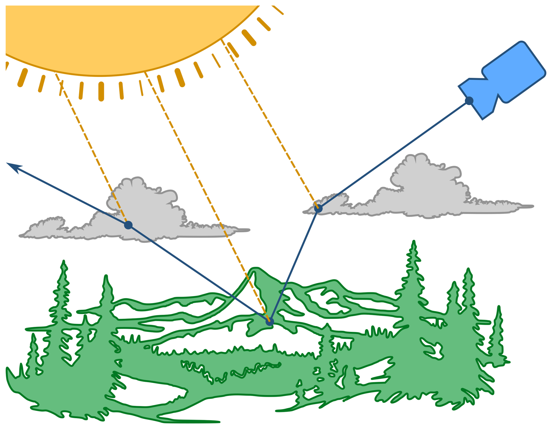
Figure 1 Eradiate uses a path tracing algorithm which builds light paths by performing random walks from the sensor, bouncing at surfaces and in the 1D atmosphere. At each node, a radiance sample is computed and added to the path contribution (this is the next event estimation method, also known as local estimate). The path is terminated if the ray escapes the medium or by the Russian roulette criterion.

In spherical-shell geometry, a flexible volumetric path tracing algorithm is used. This algorithm implements null-collision-based distance and transmittance sampling (Galtier et al., 2013; Novák et al., 2018; Miller et al., 2019), and trades off performance for flexibility. It uses a rejection technique to sample distances and estimate transmittance: this sets no constraint on scene geometry or on extinction coefficient data spatial variations and the method therefore adapts very well, in principle, to all kinds of atmospheric profiles. In practice, the method becomes less efficient at high optical thicknesses (above 1) due to the use of a global majorant for distance sampling. Several strategies are possible to overcome this issue, such as local majorants (Villefranque et al., 2019; Pharr et al., 2023) or an analytical estimator: these are areas for improvement for a future release.

4 Earth surface-atmosphere system components

4.1 Surface

4.1.1 Reflection models

The surface in the baseline scene (see Sect. 3.2) can be assigned various bidirectional scattering distribution functions (BSDFs).

The simplest reflection model provided by Eradiate is a diffuse (a.k.a. Lambertian) reflectance. The kernel-level implementation is wrapped in a high-level interface that allows specifying spectral variations with an xarray dataset object. This flexible data structure can be loaded from standard formats (e.g. NetCDF) or supplied directly by the user, who can write their own data converter very easily.

Several more complex BSDFs are available: implementations of the RPV, RTLS and Hapke models, as well as three different water surface models, are provided and can be assigned to the surface. Table 1 summarizes the intended usage of the main reflection models. Similar to the diffuse model, the kernel-level implementation of all reflection models is wrapped in a high-level interface that simplifies user input.

Rahman et al. (1993); Pinty et al. (2000)Strahler et al. (1999)Hapke (1984, 2012)Mishchenko and Travis (1997)Litvinov et al. (2024)Kotchenova et al. (2006)

Table 1 The main surface reflection models implemented by Eradiate.

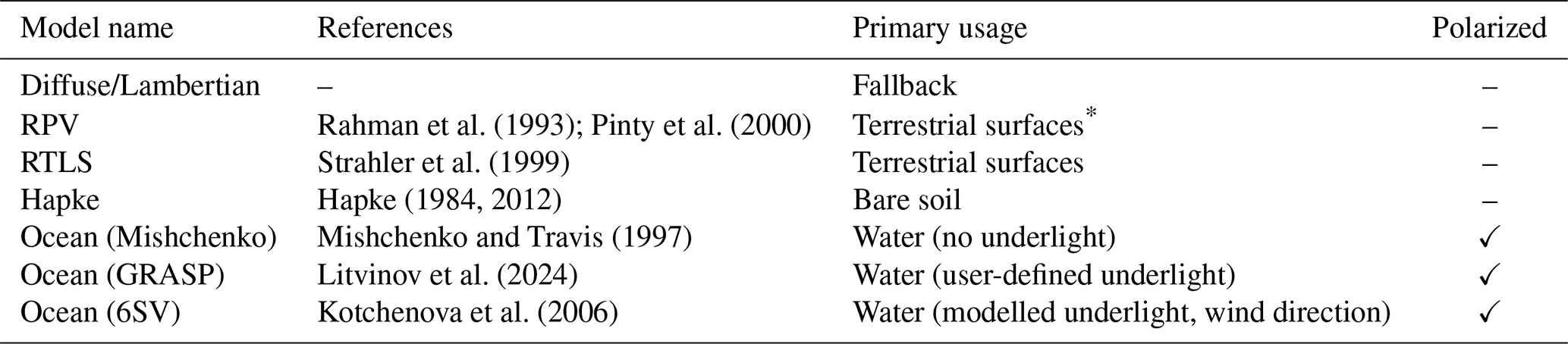
^* Primarily designed for vegetation.

4.1.2 Complex surface features (vegetation, topography)

Building on its radiometric kernel, Eradiate offers the possibility to load arbitrary shapes and assign them any reflection model implemented at the kernel level. In particular, it is possible to load triangulated meshes, which allows representing surface features of arbitrary complexity with relatively low effort and great flexibility.

All shapes can also be “cloned” with low memory cost using instancing. Instances can be positioned arbitrarily in the scene, in any number, and can be used e.g. to replicate a tree model or a forest patch many times.

These features can be used to model topography (Fig. 2), as well as explicitly resolved vegetated canopies (Fig. 3) and urban environments. Users can also use their own 3D models, and Eradiate provides specific infrastructure to load the 3D canopies defined in the RAMI benchmark series (Widlowski et al., 2007, 2015) based on PLY meshes.

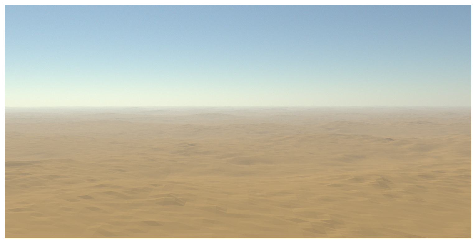
Figure 2 RGB view of the Algeria-5 pseudo-invariant calibration site with a plane-parallel atmosphere. The scene features an aerosol layer with an optical thickness of 0.2 and an exponential density distribution. The surface shape is a triangulation of the Copernicus GLO-30 (30 m resolution) digital elevation model (DEM) (Strobl, 2020) with a diffuse reflection model. See Sect. 8.2.2 for more technical details.

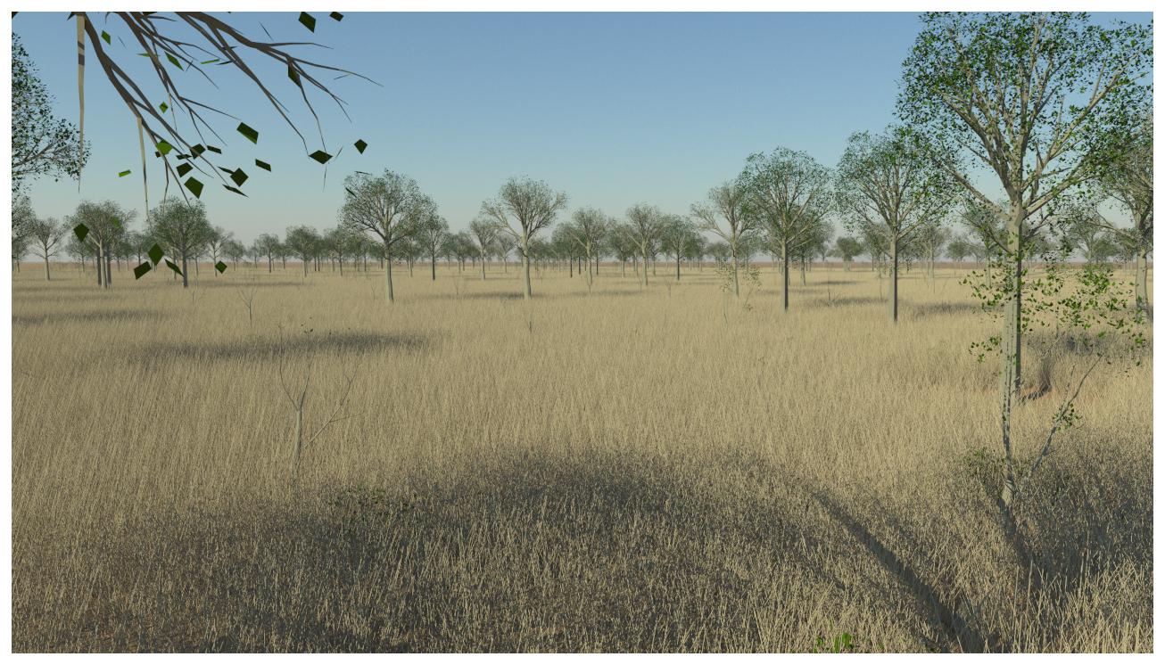
Figure 3 RGB view of the Savanna Pre-fire scene (Disney et al., 2011) with a plane-parallel atmosphere. The scene features an aerosol layer with an optical thickness of 0.1 and an exponential density distribution. See Sect. 8.2.1 for more technical details.

4.1.3 Surface texturing

Most BSDF parameters can be textured, i.e. assigned spatial variations in addition to their spectral variations. This allows one to, e.g., vary the reflectance of a diffuse BSDF at a surface. Texturing is done by mapping an object's texture coordinates (sometimes referred to uv coordinates) to a data source, typically an array with two spatial dimensions and one spectral dimension such as a spatially resolved hyperspectral albedo dataset. Figure 4 shows an example of diffuse reflectance texturing.

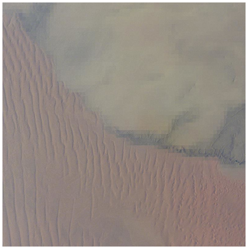
Figure 4 Nadir top of atmosphere (TOA) view of the Gobabeb HYPERNETS site in Namibia (De Vis et al., 2024) with a plane-parallel atmosphere (AFGL 1986 US Standard profile, no aerosols). The surface shape is a triangulation of the Copernicus GLO-30 DEM (30 m resolution) with a diffuse reflection model textured by a resampling at 1 km of the HAMSTER dataset (Roccetti et al., 2024).

The Eradiate kernel also ships with a “selector” BSDF plugin, which dispatches calls to multiple nested BSDF plugins, based on an index texture. In practice, this can be used to map land cover categories to associated material models, which do not have to be identical: one can assign, e.g., an RPV model to the land parts of a topographic model, and a water surface model to the water parts. Figure 5 shows an example of land cover-based material selection, as well as instancing (see Sect. 4.1.2).

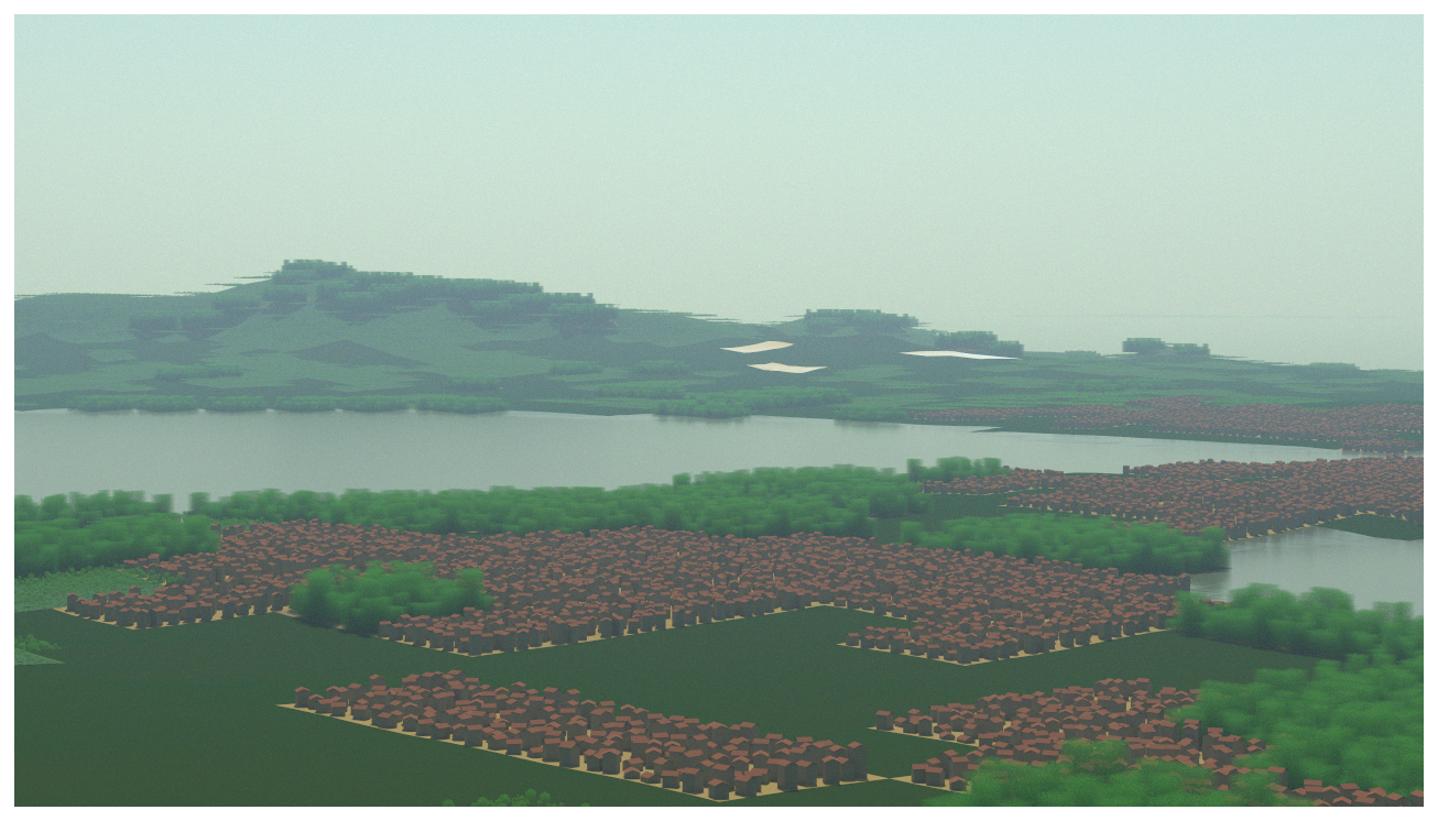
Figure 5 RGB view of a synthetic scene created after the area of Mbita, on Lake Victoria in Kenya. The surface shape (a triangulation of the Copernicus GLO-30 DEM) is assigned different reflection models (e.g. water, diffuse, RPV) based on land cover information contained in a texture encoded as a PNG image. Where relevant, land areas are also tiled with 3D objects at a reduced memory cost using instancing: a few templates (e.g. village, forest) are cloned many times to create a radiatively plausible reflection pattern. See also Sect. 8.2.3 for a similar example.

4.2 Atmosphere

The atmospheric medium is split into “molecular” (mostly gases) and “particulate” (aerosols or clouds) components. Components can be described with different vertical resolutions and are all resampled to the computational vertical grid (see Sect. 3.2). Only one molecular component is allowed, while any number of particulate components is allowed.

4.2.1 Molecules

The molecular component's optical properties are driven by a thermophysical property vertical profile that maps the temperature, pressure and species concentrations against altitude. Thermophysical profile handling tools are factored in an independent library (Nollet and Leroy, 2024) that can generate standard profiles such as the six AFGL profiles (Anderson et al., 1986), and rescale their total column concentrations to a target value, e.g. to account for the increase in CO₂ concentration since the 1980 s. Eradiate can also use arbitrary, user-supplied input, allowing for instance to derive thermophysical profiles from data provided by the Copernicus atmosphere monitoring service (CAMS) (Inness et al., 2019) for improved realism.

Molecular scattering. Molecular scattering is modelled with a polarized Rayleigh phase function (Hansen and Travis, 1974) that includes the depolarization factor to account for molecular anisotropy. When polarization is neglected, the (1,1) element of the phase matrix serves as the scattering phase function.

Molecular absorption. The thermophysical profile is used to query a molecular absorption database and build an absorption coefficient vertical profile. At the time of writing, Eradiate ships with 6 molecular absorption databases created from the HITRAN 2020 spectroscopic database (Gordon et al., 2022) using the RADIS (Pannier and Laux, 2019) software package. Additional cross-section data, not found in HITRAN's absorption line database (e.g. ozone photodissociation data published by Gorshelev et al., 2014; Serdyuchenko et al., 2014) are also incorporated in the shipped cross-section databases. Users can use their own molecular absorption data, provided that it complies with the documented data format. Table 2 lists all shipped databases.

Table 2 List of Eradiate's shipped molecular absorption databases.

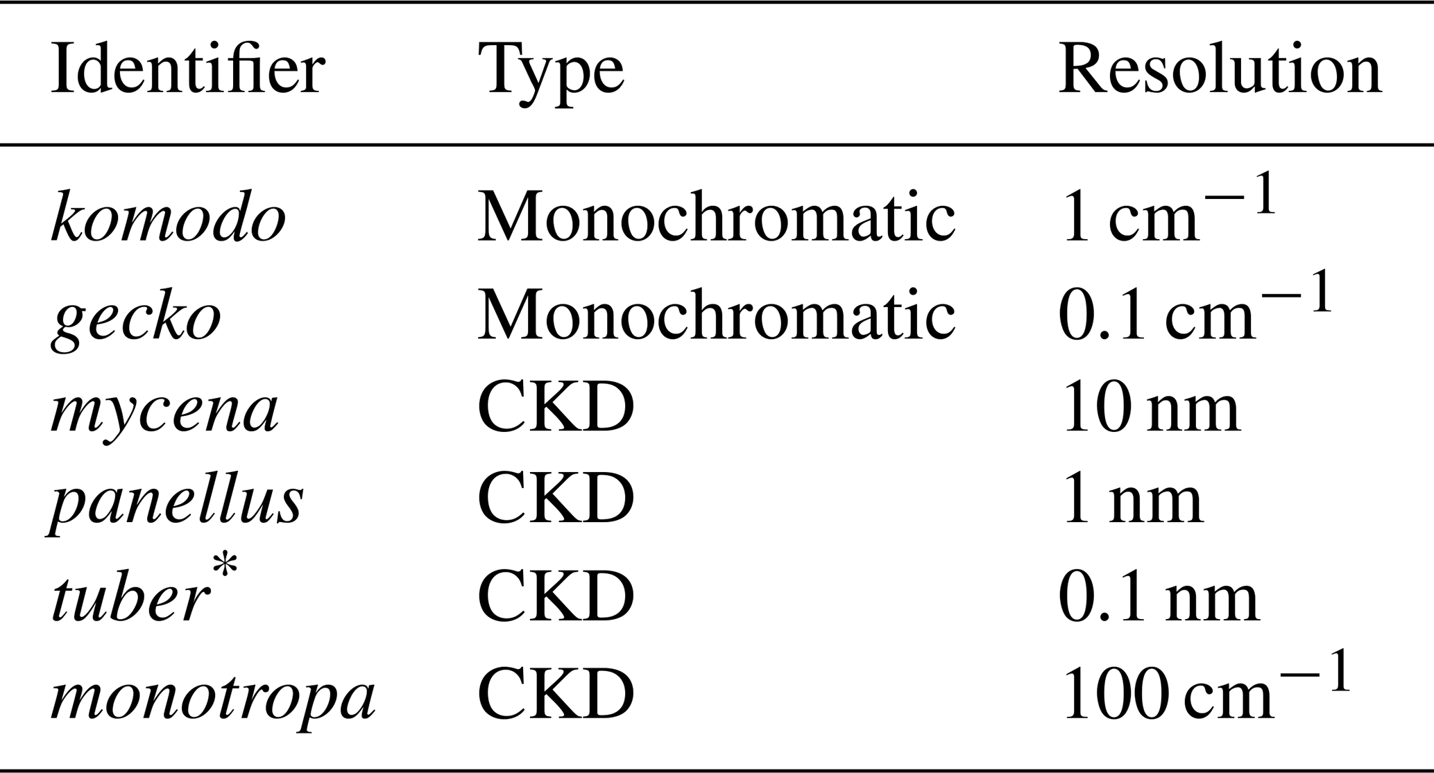
* Only covers the [250,2550] nm interval.

Eradiate can process the spectral dimension using two methods, which are selected upon activation of the operational mode:

• In monochromatic mode, the user inputs the sequence of wavelengths for which the RTE is solved. In that mode, the atmospheric absorption database (either brought by the user or selected from the list of built-in monochromatic databases mentioned in Table 2) should have a spectral resolution that is fine enough to resolve the complex line structure of the molecular absorption spectrum.

• In CKD mode, the spectral dimension is handled using the CKD method. Eradiate mostly follows the terminology of Hogan and Matricardi (2020). The spectrum is divided into a a set of spectral intervals, known as bins. This method alleviates the need to cover very densely the spectral dimension to resolve the high-frequency spectral features of molecular absorption spectra by reordering absorption coefficient values (denoted k) in each bin against a pseudo-frequency (denoted g) that represents the cumulative probability of the absorption coefficient over that bin. The resulting function k(g) is monotonically increasing and smooth, which allows to compute spectral integrals using a low-order quadrature rule (typically Gaussian) with good accuracy. The quadrature points are called g-points. In practice, this reduces by several orders of magnitude the number of spectral samples to process to achieve satisfactory accuracy. For further detail on this method, see, e.g., Lacis and Oinas (1991). In the CKD mode, the spectral discretization is driven by the selected absorption coefficient database. The bins that will be processed during the simulation are selected either manually by the user, or based on the sensor's spectral response function. When launching the simulation, Eradiate solves the RTE for each g-point of each active CKD bin, then aggregates each bin's g-points using the specified quadrature rule.

Monochromatic absorption databases are indexed by wavelength, pressure, temperature and species concentrations. Samples covering the solar reflective region (250 nm to 3 µm) are available through the data management interface. To restrict the amount of data delivered to a reasonable amount, these databases are sparse in all dimensions and are not recommended for quantitative applications. Providing a database with a higher spectral resolution is however possible.

CKD absorption databases are provided for the same spectral region with four spectral resolutions (see Table 2). Like their monochromatic counterparts, the CKD databases feature pressure, temperature and species concentration dimensions. Two spectral dimensions are used: each CKD bin is identified by its central wavelength, and the absorption coefficient is then indexed by the g pseudo-spectral coordinate in the CKD method. This indexing method allows to store a highly resolved k-distribution, giving flexibility in how g-points can be chosen during computation. Eradiate uses a conservative setup with a 16-point Gaussian quadrature, but other quadrature rules or number of g-points are supported.

4.2.2 Aerosols

The aforementioned molecular component can be combined with an arbitrary number of aerosol (or other particulates) layers parametrized by a vertical extent, a total optical thickness at a reference wavelength, a vertical density distribution and a dataset describing, as a function of the spectral coordinate, the single-scattering properties for that layer (extinction coefficient, single-scattering albedo, and phase matrix). Such single-scattering properties can be computed from microphysical properties, e.g. using Mie theory (for spherical particles) or the T-matrix method (for non-spherical particles).

Eradiate ships with a few sample datasets, and notably includes the aerosol classes defined by the 6SV RTM. No tool is included to derive single-scattering properties, but Eradiate can import data in the NetCDF format supported by the libRadtran RTM: Thus, users can provide customized input generated, e.g., using the MOPSMAP online tool (Gasteiger and Wiegner, 2018), or libRadtran's mie tool (Emde et al., 2016).

4.2.3 Clouds

Eradiate also supports cloud modelling, under the 1D assumption, using the same framework as for aerosols. Single-scattering properties therefore have to be supplied to the model, and can be derived from microphysical properties using Mie theory for liquid water clouds. Data for ice clouds based on appropriate parametrizations can also be imported, e.g. from libRadtran. 3D clouds are not supported by this release, but their addition is planned in a future version.

4.3 Illumination

Top of atmosphere irradiance spectrum. Several irradiance spectra are provided (Thuillier et al., 2003; Woods et al., 2009; Haberreiter et al., 2017; Meftah et al., 2018) and normalized to 1 AU, with the CEOS-endorsed TSIS-1 spectrum (Coddington et al., 2021) as the default. For more accurate radiance simulations, irradiance values can be scaled to account, e.g., for seasonal variations due to the eccentricity of the Earth's orbit around the Sun. The irradiance spectrum class accepts user-defined input in the documented format.

Illumination model. Eradiate provides two illumination models that describe radiance boundary conditions at the outer boundary of the computational domain, giving the value of the radiance field as a function of direction. The first one, a perfectly directional model, describes the radiance distribution as a delta Dirac distribution. The second one is more realistic and accounts for the fact that solar illumination, at the top of the atmosphere, is not perfectly directional, and implements in practice an environment map, also known as infinite area light in computer graphics (Pharr et al., 2023). Both illumination models are parametrized by the local solar zenith and azimuth angles and the selected irradiance spectrum. Figure 6 illustrate the conceptual difference between the two models.

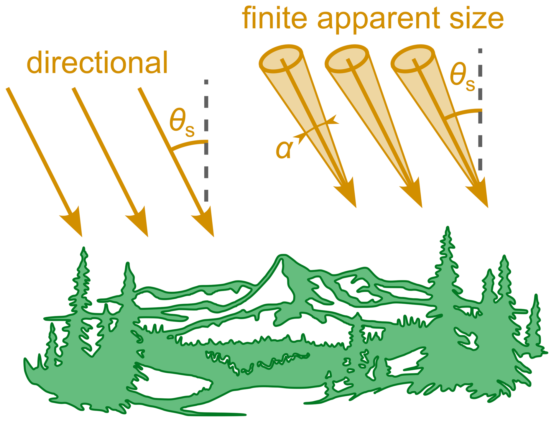
Figure 6 An illustration of Eradiate's illumination models. The first model (left) is perfectly directional and parametrized by the solar zenith (θ_s) and azimuth angles; the second (right) models the Sun's finite apparent size α, in addition to the solar angles.

5 Sensors and measurements

Most sensors implemented by Eradiate can be positioned arbitrarily in the scene. It is therefore possible to simulate measurements at the top of the atmosphere (e.g. to model a satellite), at the bottom of the atmosphere (ground level, e.g. to model a camera or a sun photometer), or anywhere in between (e.g. to model an airborne radiometer).

5.1 Fundamental radiometric quantities (radiance, fluxes)

Eradiate provides several sensors that offer interfaces to sample radiance at the aforementioned locations, varying the pixel count, angular coverage or spatial sampling – depending on what is most appropriate for the targeted application.

A simple radiancemeter allows to record radiance in a single direction from an arbitrary position in the scene. The interface allows to define several such sensors (positioned at different locations and pointing to different directions) that will be processed in parallel.

Another variant targets a specific location in the scene from a distant location. This distant radiancemeter also exists in several versions, which have various angular parametrizations (discrete or continuous). The distance between the target location and ray origins can be adjusted, up to infinity, making this sensor family a very flexible tool for computing various kinds of radiance estimates.

A special variant of the distant radiancemeter records the directional flux leaving a target location defined by an arbitrary positioned and oriented flat surface. It can, in practice, be used to compute the directional or total flux reflected by a surface.

Finally, a perspective camera sensor can be used as a more traditional interface to generate images. It implements a pinhole camera model with a configurable field of view.

These fundamental radiometric quantities can be combined to simulate more complex measurements. Section 8 provides a few examples that use one or multiple sensors.

5.2 Spectral response

All sensors can be assigned a spectral response function (SRF). Two main spectral response types are available:

• The delta spectral response selects one or several wavelengths in the spectrum at which Eradiate performs radiometric computations. In monochromatic modes, the exact wavelength is processed; in CKD modes, the CKD bin that includes the selected wavelength is processed. Results obtained with a delta SRF are not applied spectral weighting (a.k.a. convolution).

• The band spectral response applies an instrument spectral response function. Eradiate performs radiometric computations on the spectral domain covered by the SRF data, and outputs both the raw radiometric output, and the SRF-weighted radiometric quantities.

Eradiate ships with a library of band SRF data, and the documented xarray dataset format allows users to easily add their own.

6 Architecture and design

Eradiate is written in the Python 3 and C++17 languages. It consists of a high-performance radiometric kernel driven by an interface layer. The radiometric kernel uses low-level abstractions to run simulations; the interface layer exposes higher-level abstractions to the user, builds and runs simulations, then collects the results and packages them in a convenient format (see Fig. 7).

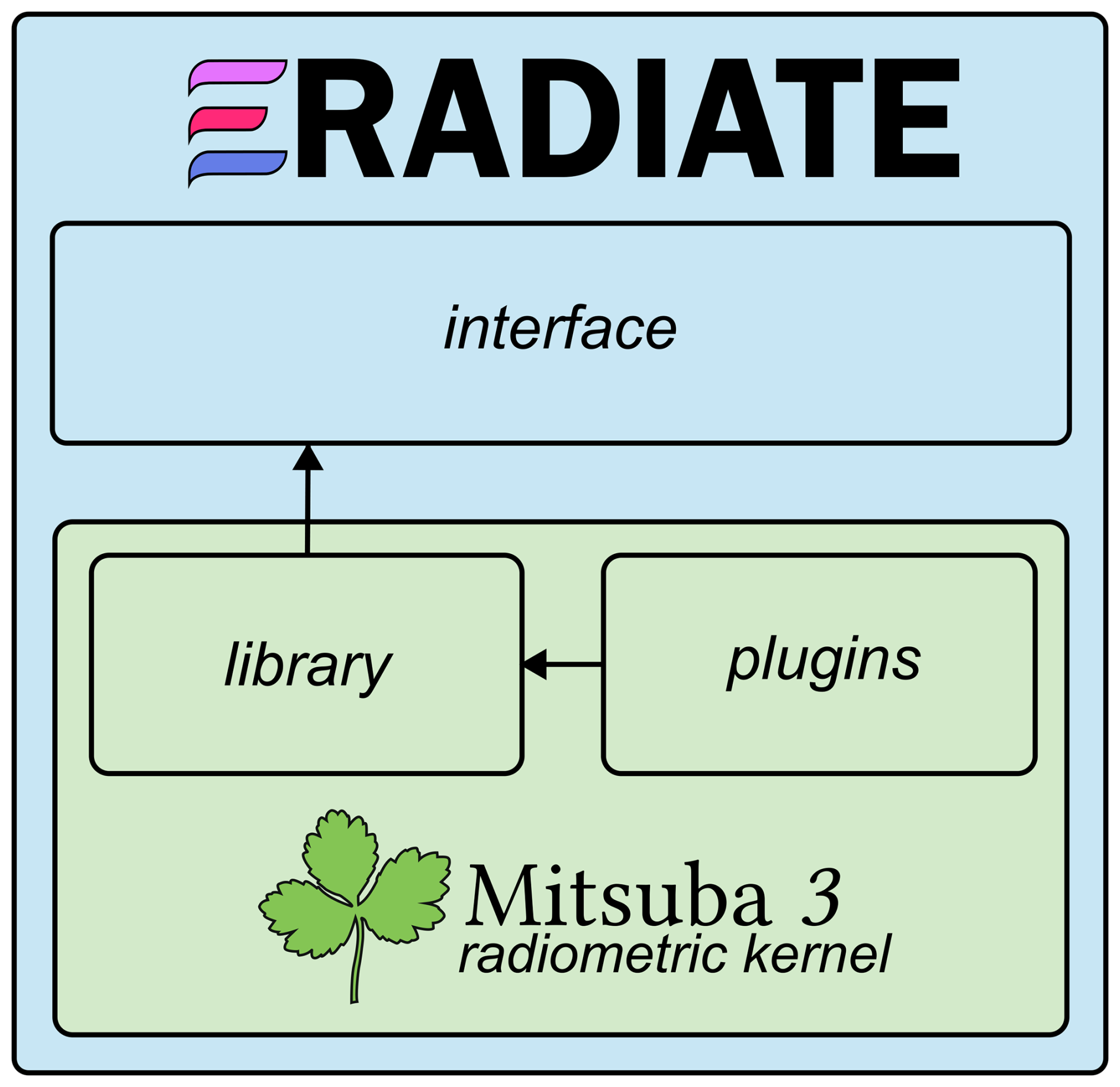
Figure 7 Architectural overview of Eradiate. The user-facing Python interface wraps a modified version of Mitsuba, our radiometric kernel, through its Python interface. The Python interface exposes library components written in C++ through extensive bindings. Mitsuba plugins, written in C++ or Python, implement kernel-level models and algorithms.

6.1 Radiometric kernel: Mitsuba 3

Eradiate's radiometric kernel is a modified version of Mitsuba 3 (Jakob et al., 2022a), a research-oriented rendering system written in C++ and Python. Its architecture shares similarities with that of PBRT (Pharr et al., 2023), which simplifies the learning curve despite the large number of advanced features it implements. Using an existing open-source renderer as the radiometric kernel, instead of writing a dedicated piece of software, dramatically reduces the amount of work required on foundational infrastructure (e.g. ray-shape intersections with built-in k-d tree or BVH construction, optical property representation, MCRT algorithm implementation). Mitsuba is built by trained computer scientists on the basis of proven architecture and takes advantage of utility libraries that ensure excellent performance. Its community of users and contributors helps to detect and solve issues and provide software usage examples.

Mitsuba is a retargetable system: its codebase is written with C++ template metaprogramming, which allows performing compile-time code transformation varying fundamental aspects of the renderer. This notably includes varying colour representation (e.g. monochromatic, RGB or spectral), accounting for polarization and changing floating point number precision. The renderer is built on top of the Dr.Jit just-in-time compilation library (Jakob et al., 2022b), which provides various computational backends targeting CPU or GPU hardware, also selectable through template metaprogramming. Each combination of template parameters is called a variant; compiled variants are defined at the beginning of the build process, and the active variant is selected at runtime. Eradiate takes advantage of this aspect of Mitsuba which greatly reduces the amount of code to maintain. For example, our polarized reflection and scattering algorithms are all implemented as variants of an unpolarized baseline in a unified codebase.

Mitsuba has a modular architecture: a core library provides basic infrastructure and interfaces, and the implementation of most of the algorithms involved in the MCRT process is contained in plugins dynamically loaded at runtime. Core library components and interfaces are generally stable and rarely require deep changes: thus, the API changes made in Eradiate's modified version of Mitsuba are carefully pondered to reduce the overhead when integrating upstream updates, which happen frequently due to Mitsuba's research software status. On the other hand, Eradiate's kernel contains a lot of plugin code that complements Mitsuba's shipped plugins with remote sensing-oriented components that implement specialized algorithms and models.

Mitsuba provides a set of fine-grained Python bindings which grant full access to most of the components of the renderer. The completeness of this Python interface was decisive when selecting the renderer to use as our radiometric kernel: the radiometric kernel can be entirely controlled in the language used to implement the interface layer.

6.2 Basic concepts

Mitsuba's variant selection system propagates to Eradiate in the form of operational modes. The active operational mode is selected globally and defines how the spectral dimension is handled (monochromatic or CKD), and whether polarization is accounted for. Eradiate currently operates entirely in double-precision to accommodate easily the potentially huge characteristic length scale differences there can be between the largest (a planet and its atmosphere) and smallest (a tree leaf or grass blade) objects in the simulation. Each mode is identified by a single keyword (e.g. mono or ckd_polarized).

Eradiate defines simulations using objects called experiments and formalized by the Experiment interface. An experiment class automates the assembly of a scene which consists of geometric primitives, surface and volume scattering properties, illumination and measure models, and an RTE integration algorithm, referred to as scene elements in the following.¹ The Experiment base type is subclassed to provide an interface that has a scope limited to a specific type of problem.

Experiment initialization does not trigger the simulation: the experiment object is created by the user and only holds a configuration until the eradiate.run() function is called. At this point, the scene assembly process is triggered, the experiment is translated into a kernel dictionary – the input to the Mitsuba radiometric kernel – depending on the active operational mode, and a Mitsuba scene object is instantiated. Eradiate then takes advantage of Mitsuba's scene update system: a Mitsuba scene object exposes scene parameters that can be dynamically updated while maintaining scene state consistency. In particular, the spectral properties of objects can be changed without triggering a full scene reload. Eradiate leverages this to run a sequence of monochromatic simulations in a so-called spectral loop. Each iteration of the spectral loop produces monochromatic output data held by a Mitsuba bitmap object. Collected bitmaps are aggregated into an xarray (Hoyer and Hamman, 2017) data structure (Fig. 8).

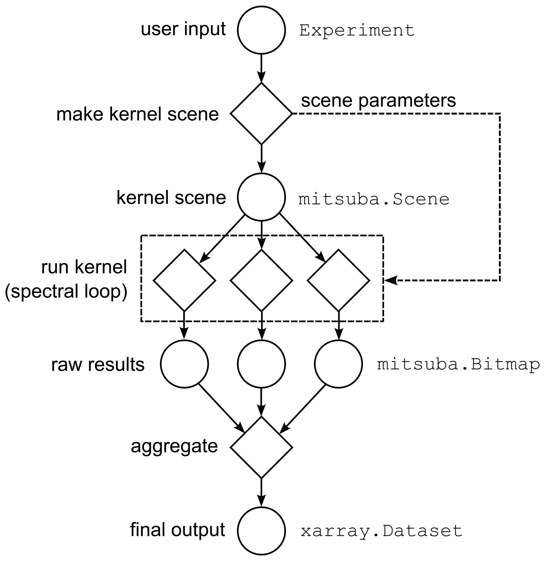
Figure 8 Eradiate's processing pipeline pre-processes user input, issued as an Experiment object, and generates a kernel scene dictionary, itself turned into a Mitsuba Scene object. The Mitsuba renderer is called repeatedly in a sequence where each iteration corresponds to a point in Eradiate's spectral discretization. The resulting raw output is then post-processed and formatted as an xarray dataset.

6.3 Scene assembly

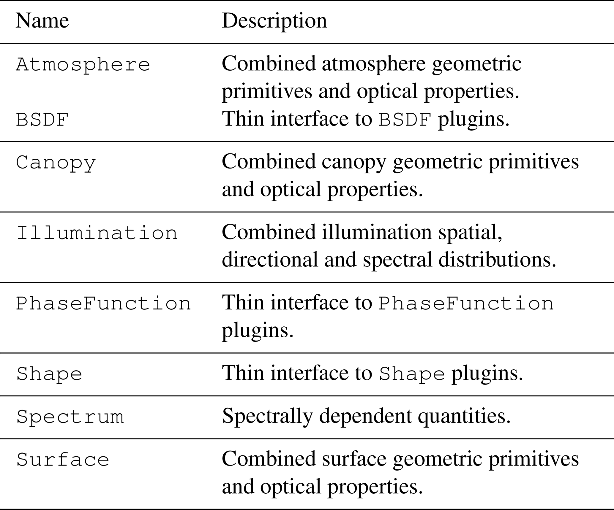
Simple interface. Eradiate's scene assembly process is centred around scene elements. They can represent geometric primitives, optical properties, illumination conditions, measures or MCRT algorithms. Various interface classes are defined, then implemented by concrete classes. They are generally independent of each other, acting as wrappers around one or several Mitsuba plugins. Coupling between scene elements generally occurs on an Experiment-dependent basis. For instance, a measure's target area may be constrained by the geometry of the problem: the Experiment object will then take care of making sure that the geometry and measure definitions are compatible with each other, and either automatically correct the configuration, warn the user or fail (i.e. raise an exception).

Scene assembly components are categorized thematically. Each general scene element class is embodied by an interface (see Table 3), itself implemented by various concrete classes. Although combining scene elements arbitrarily is conceptually possible, their assembly is constrained by their parent Experiment. For instance, a user will not be allowed to add multiple molecular atmospheric components at the same time.

Table 3 List of Eradiate's main SceneElement interfaces.

Expert interface. Simulations of complex scenes are generally out of the scope of the constrained simple interface defined by Experiment classes. For such situations, Eradiate offers the possibility to users to define their input using low-level Mitsuba primitives directly. When inserting such objects, users must pay attention to scene consistency themselves, but are in exchange free to do anything the radiometric kernel allows. The expert interface extends the baseline Experiment interface with two kinds of input:

• Mitsuba scene input, either in the form of full or partial kernel dictionaries, or fully initialized Mitsuba objects;

• scene parameters, which describe how Mitsuba scene parameters are updated at each iteration of the spectral loop.

A scene parameter definition includes:

• the parameter update protocol in the form of a callable that takes as input spectral loop contextual data;

• additional metadata used to associate the update protocol with a node in the Mitsuba scene parameter tree.

This infrastructure is what powers internally the simple interface and allows power users to use all Mitsuba plugins in their customized setup, including those which are not exposed by any Eradiate scene element. User kernel dictionary and scene parameter definitions are merged with the ones generated by the simple interface upon experiment initialization.

Appendix C elaborates on Eradiate's user interface and provides examples of simple and expert interface scripting.

7 Validation and benchmarking

As mentioned earlier, Eradiate is intended to provide a highly accurate simulation framework suitable for cal/val applications and is validated against both analytical test cases, community-approved benchmarking results and actual measurements.

7.1 Analytical solutions and unit testing

The first validation stage consists in checking Eradiate's output against known analytical solutions. While full radiative transfer simulation scenarios are generally too complex to derive an analytical solution, many components in the software package can be validated individually. This notably includes the evaluation and sampling routines of most scattering models, as well as the scene assembly process. These tests are implemented as part of Eradiate's unit testing framework, based on pytest (Krekel et al., 2004), which is run frequently on the development branch to detect regressions.

7.2 RAMI benchmark series

RAMI Online Model Checker (ROMC). Eradiate's canopy simulation features are validated against scenarios defined for the ROMC tool² (Widlowski et al., 2008). It provides a framework for autonomous canopy RTM benchmarking based on scenarios developed during the first three phases of the Radiative transfer Model Intercomparison (RAMI) (Pinty et al., 2001, 2004; Widlowski et al., 2007). ROMC scenarios are based on abstract canopies with diverse structures, e.g. homogeneous vegetated covers with different leaf angle distributions, clusters of spherical leaf clouds, or more realistic setups similar to forests. Canopy definitions are general, leaving to users and their RTM the choice of the representation: We chose to represent leaves as disks, but similar performance could be achieved by representing them using triangulated meshes. Readers interested in a complete list and description of the ROMC scenarios are referred to the original RAMI-3 publication (Widlowski et al., 2007) and the RAMI website.³

ROMC users can submit simulation results for various measurements: top of canopy (TOC) bidirectional reflectance factor (BRF) (full contribution, as well as partial contributions accounting for various orders of scattering or ignoring reflection by specific objects in the scene), fraction of radiation absorbed by foliage, albedo and flux transmitted through the canopy. ROMC submissions can be done in two modes:

• The DEBUG mode allows repeated submissions on many scenes and reveals to the user a reference against which they can compare and adjust. This mode is designed to help RTM developers debug their code to reach the community consensus.

• The VALIDATE mode allows only one submission on a restricted set of randomly chosen scenes different from those available in DEBUG mode, and exposes no “ground truth” for comparison before submission is completed. This mode is designed as a blind exercise to allow RTM developers and users to get a traceable proof of the performance of their model.

Eradiate was used to simulate the BRF in the principal and orthogonal planes.⁴ The full, single- and multiple-scattering contributions were computed. Periodic boundary conditions were simulated by padding the unit cell with instances of itself. The number of padding rows required to converge to a quasi-periodic setup depends on the scene. For the tested scenes, a padding value of 20 was appropriate. Various submissions were done in DEBUG mode, presented in Appendix A. A VALIDATE mode run was also performed, with results shown in Table 4. The skill score (as defined by Widlowski et al., 2008) on the submitted measurements is generally high (99 % or higher). The only exception is the brfpp_mlt measurement (multiple scattering in the principal plane) which is computed from three combined Monte Carlo estimators and thus accumulates variance: this results in increased noise, particularly visible when the expected value is low (all scenarios except HET41_DIS_ERE_NIR_30), and degrades the skill score. This measurement is however correct when the expected value takes more significant values (see the HET41_DIS_ERE_NIR_30 scenario). Lower variance could be achieved by implementing an integrator that returns this measurement directly.

Table 4 Eradiate ROMC submissions (model name: eradiatev100) in VALIDATE mode. Visuals are representative of the mentioned scenes, but not accurate renders of the particular simulated variants (e.g. the HET01 and HET41 scenes feature different numbers of spherical leaf clouds).

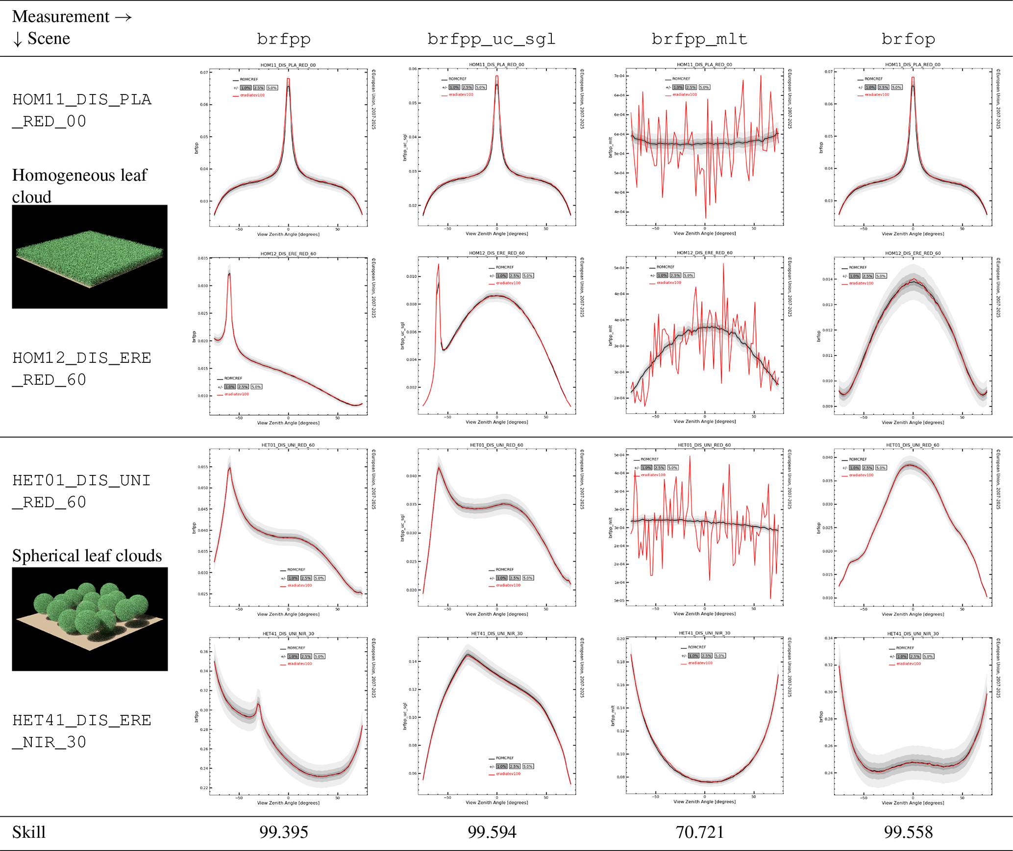
brfpp: BRF in the principal plane.
brfpp_uc_sgl: BRF in the principal plane for single-scattered radiation collided by the soil.
brfpp_mlt: BRF in the principal plane for multiple-scattered (two or more scattering events) radiation.
brfop: BRF in the cross plane (perpendicular to the principal plane).

From this, we conclude that Eradiate performs well on a variety of discrete scenes to compute radiance estimates. Remaining issues are attributed to operator mistakes, i.e. incorrect scene or measure setup.

Other RAMI phases. In addition to the permanently open ROMC, Eradiate was used to contribute to the RAMI-V and RAMI4ATM phases. RAMI-V (Lanconelli et al., 2025) further increases the complexity of canopy-centric benchmarking scenarios, with multiple scenes derived from actual canopies. At that time, Eradiate's canopy simulation features were in an early development stage and the submission was partial, focusing on a single scene and reflectance measures. The submitted results were within good agreement with other well-established MCRT models such as DART or LESS.

The RAMI4ATM phase (Joint Research Centre, 2025), in progress at the time of writing, focuses on benchmarking RTMs targeting 1D atmospheric simulation. Eradiate's coverage for that phase is much more extensive.

Relationship with unit testing. A few scenarios derived from the RAMI scenario pool were turned into regression tests and are executed as part of Eradiate's regular unit test suite using a statistical testing framework, mitigating the risk of regression without the need to run complete benchmarks.

7.3 IPRT benchmark series

In order to validate Eradiate for polarimetric simulations including scattering from molecules, aerosol particles and cloud droplets in the Earth atmosphere, we compared against comprehensive benchmark results established by the International Working Group on Polarized Radiative Transfer IPRT (Emde et al., 2015). The first phase of IPRT includes 1D setups for clear atmospheres, for cloud and aerosol scattering, as well as for surface reflection. The benchmark results were established by intercomparison of six participating independently developed radiative transfer codes.

Figure 9 shows the Eradiate results for case B3. The simulation uses the US Standard Atmosphere (Anderson et al., 1986) together with a typical aerosol profile (Shettle, 1986), with a vertical aerosol optical thickness of 0.2. Aerosol optical properties are provided on the IPRT website⁵ and correspond to prolate spheroids with an aspect ratio of 3. The particle size distribution has a mode radius of 390 nm. The complex refractive index is 1.52−0.01i and the mass density is 2.6 g cm⁻³. These properties are representative of the coarse mode of mineral dust aerosols (Hess et al., 1998). Simulations are performed at a wavelength of 350 nm in the ultraviolet spectral region, where Rayleigh scattering is strong and absorption is dominated by ozone. Radiances are calculated for sensors located at the surface, at 1 km altitude, and at the top of the atmosphere (TOA). The figure can be directly compared with Fig. 8 in Emde et al. (2015). The upper panels show the radiation field for a sensor at TOA viewing downward, while the lower panels show the radiation field for a surface sensor viewing upward. The solar zenith angle is 30° and the solar azimuth angle is 0°. The solar position is indicated by a yellow star in the polar plots. The subplots display the Stokes vector components: the intensity I, the linear polarization components Q and U, and the circular polarization component V. In this case, V is three to four orders of magnitude smaller than the linear polarization components. At the surface, the intensity I exhibits a pronounced forward-scattering peak in the solar direction. The degree of polarization is largely controlled by Rayleigh scattering and reaches its maximum at scattering angles close to 90°.

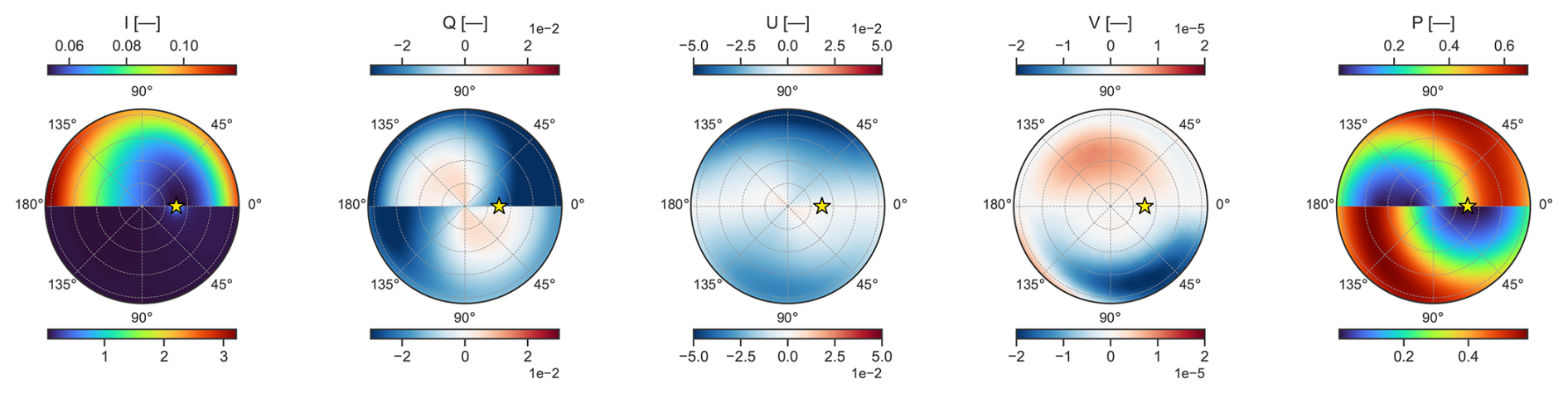
Figure 9 Simulated radiance field (Stokes components and degree of polarization P) at 350 nm for a standard atmosphere and vertically inhomogeneous aerosols with an optical thickness of 0.2. The upper part of the figures represents the radiance field at the top of the atmosphere for down-looking directions, and the bottom part is for up-looking directions at the surface. The I, Q, U and V fields are normalized by the incident top-of-atmosphere irradiance, which means that all quantities are unitless.

Table 5 shows the relative root mean square differences between Eradiate and MYSTIC (corresponding to Tables 3 and 4 in Emde et al., 2015). All cases except A5 were run with 10⁸ samples, for A5 including the cloud layer 10⁷ samples were used. Overall, we find a very good agreement with relative root mean square differences below 0.1 % for intensity and linear polarization. Larger differences are found for cases including clouds because less samples were run due to the high computational time caused by enhanced multiple scattering in clouds. Moreover, Eradiate does not include sophisticated variance reductions for cloud scattering so far. Nevertheless, for the intensity, the relative root mean square difference is still smaller than 0.5 %, and larger for the polarization because Q, U and V are very small for the cloud case. The differences are comparable to those of TROPOS, a Monte Carlo code without specific variance reduction methods for cloud scattering.

Table 5 Relative root mean square differences in per cent between Eradiate and MYSTIC for 1D IPRT cases published in Emde et al. (2015).

7.4 Comparison against experimental measurements

In addition to validation against analytical references and other trusted RTMs, Eradiate was compared to experimental measurements.

A validation exercise was conducted against SI-traceable reflectance measurements on an well-characterized artificial target (Leroy et al., 2025a). The target was measured optically with an SI-traceable spectro-goniophotometer, and the experiment was digitally replicated with Eradiate using as much information as possible from the experimental setup. The collected radiometric records, as well as the corresponding simulations, were attached uncertainty that allowed for comparison following metrological guidelines. The simulated reflectance values were found to agree with the experimental records within 2 % in most cases. Given the unbiased nature of Eradiate's MCRT methods, the error is mostly attributable to the accuracy of input data, in a broad sense (e.g. the selected surface scattering model and its parameters, the 3D model's geometric description, or the light source and sensor models). That exercise gave an order of magnitude of the accuracy that can be expected from a simulation in a highly controlled setup without volumetric scattering.

Eradiate was also used to produce a hyperspectral radiometric calibration reference for satellite-borne instruments (Luffarelli et al., 2025). In that study, volumetric scattering plays an important role and, although the selected calibration targets are very stable desert pseudo-invariant calibration sites (PICS), their optical characterization is very challenging. The simulation setup (notably relying on a spherical-shell geometry and detailed atmospheric molecular profiles sourced from CAMS) allowed to consistently reproduce measurements from various multispectral and hyperspectral instruments with an accuracy of 3 % or better in spectral regions where the atmospheric molecular transmittance is higher than 0.8, showing the suitability of Eradiate for that type of use case.

8 Applications and results

In this section, we demonstrate some of Eradiate's capabilities with simple examples pertaining to actual 1D and 3D use cases. Most of these examples are available as reproducible Jupyter notebooks shared in a companion repository.⁶

8.1 1D simulation

8.1.1 Calculation of radiance spectrum at top of atmosphere

To simulate hyperspectral satellite observations, we employ the correlated-k distribution database panellus (1 nm resolution, see Table 2) to generate spectra at a resolution of 1 nm. The example notebook⁷ illustrates how to set up such a simulation using the US Standard Atmosphere together with representative continental aerosol particles. For the lower boundary condition, we apply a spectrally dependent Lambertian surface albedo representative of a desert environment, extracted from the HAMSTER database (Roccetti et al., 2024).

Figure 10 presents the results. The top panel shows the solar irradiance spectrum measured by TSIS-1 (Coddington et al., 2021), which was used as input for the simulations. The bottom panel displays the TOA radiance spectra for a viewing geometry defined by a zenith angle of 60° and an azimuth angle of 75°. The corresponding solar zenith and azimuth angles are 30 and 160°, respectively. The blue line represents the TOA radiance for the US Standard Atmosphere (Anderson et al., 1986). The red line, which shows lower radiance values, includes an additional aerosol layer between 0 and 3 km altitude with an optical thickness of 2, superimposed on the molecular atmosphere. The aerosol optical properties correspond to the “continental” aerosol type in the 6S radiative transfer model (Kotchenova et al., 2006). The simulated spectrum clearly reveals the oxygen A and B absorption bands centred near 760 and 686 nm, respectively. Absorption features around 580 and 950 nm are associated with water vapour. Eradiate also provides the variance of the simulated radiance, from which the standard deviation can be derived. The shaded region indicates two standard deviations. This uncertainty is clearly non-negligible in the simulation that includes aerosols, whereas it is very small and not visible in the molecular-only case. The standard deviation scales with the square root of the number of samples, which was set to 100 in these calculations.

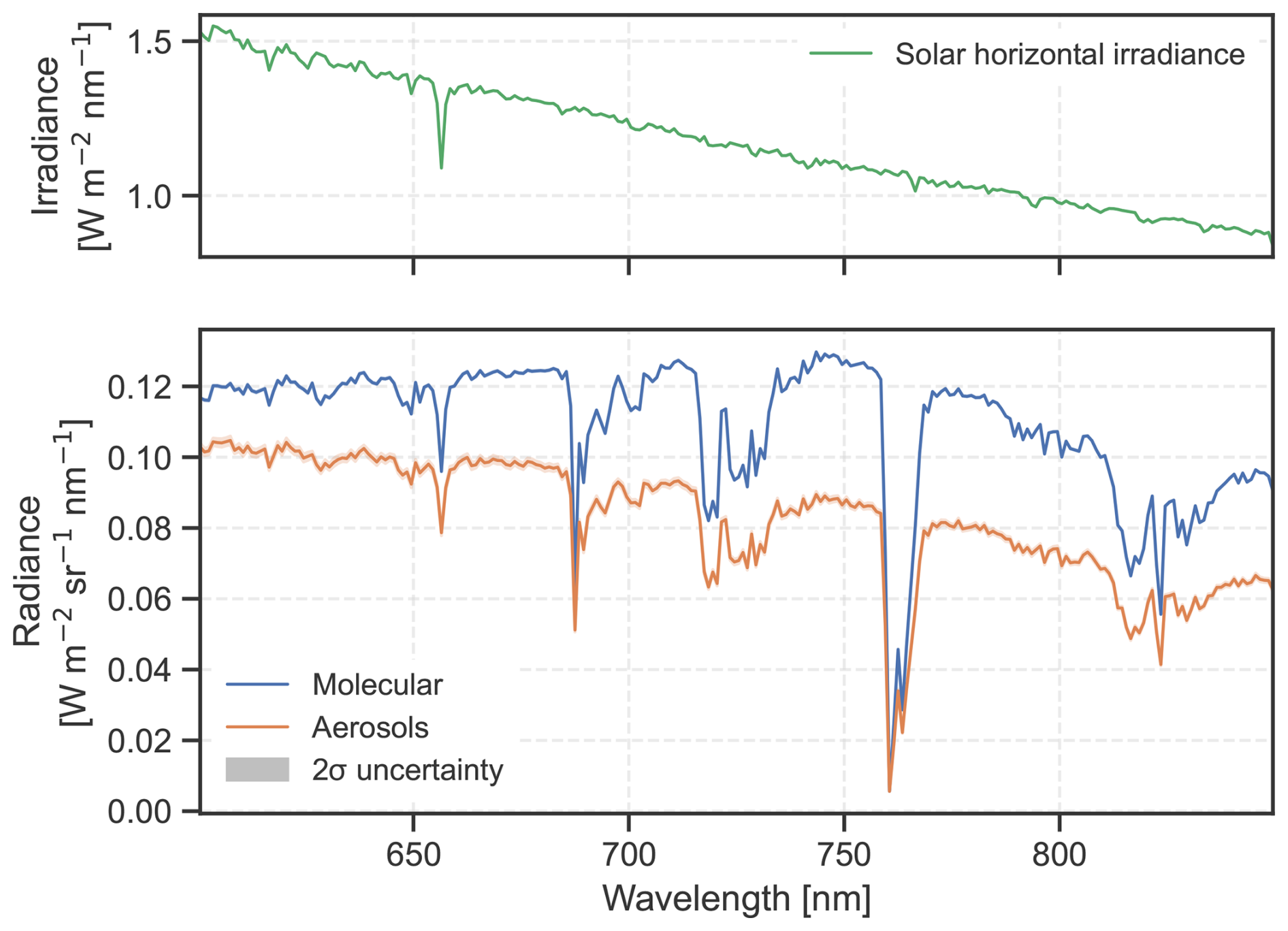
Figure 10 Top: Solar horizontal irradiance spectrum (which factors in the solar zenith angle). Bottom: Reflected radiance spectrum using the panellus absorption parametrization with a spectral resolution of 1 nm.

8.1.2 Sun photometer

AERONET (AErosol RObotic NETwork) (Holben et al., 1998) is a global network of ground-based sun photometers designed to measure aerosol optical properties. These instruments record direct solar irradiance and polarized sky radiances at multiple wavelengths across the visible and near-infrared spectral range. The example notebook⁸ demonstrates how Eradiate can be used to simulate such observations for an atmosphere containing an aerosol layer with an optical thickness of 0.5. The simulation is performed at the centre wavelengths of a typical sun photometer.

Figure 11 shows the results of a simulated almucantar scan. In this example, polarization effects are included, and the figure displays the total intensity I, the Stokes parameters Q and U, and the degree of polarization. The intensity peaks near the solar direction due to the strong forward scattering by aerosol particles. The degree of polarization decreases with increasing wavelength, reflecting the decrease of Rayleigh scattering, which is the dominant source of polarization.

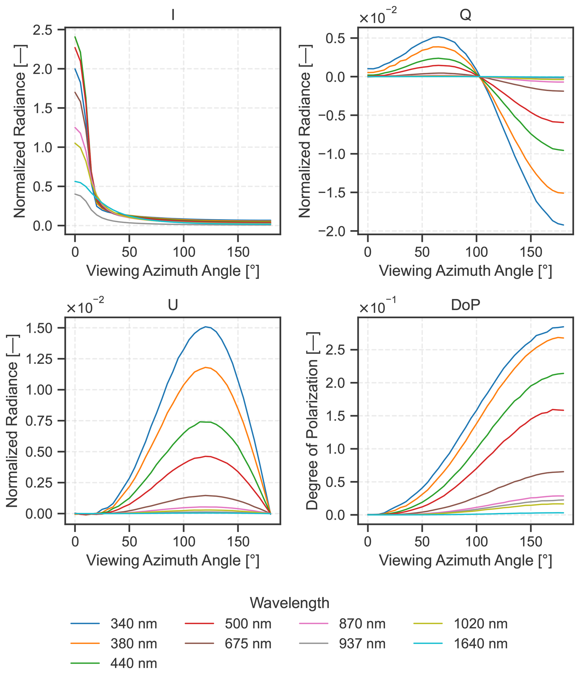
Figure 11 Simulation of radiance at the ground in the solar almucantar plane. The solar zenith angle is 30°, the surface albedo is 0.05 and the AOT is 0.5. The I, Q and U fields are normalized by the incident top-of-atmosphere irradiance, which makes results comparable across wavelengths.

8.1.3 Spherical geometry

Eradiate supports simulations in fully spherical geometry. This implementation has been validated against benchmark results published by Korkin et al. (2022). While spherical geometry is essential for limb or twilight observations, it is also critical for radiance simulations of polar-orbiting satellites, where neglecting atmospheric sphericity can introduce significant errors.

The example notebook⁹ demonstrates this effect. We include the US Standard atmosphere and compute TOA radiances for a solar zenith angle of 60° in both plane-parallel and fully spherical geometry. Figure 12 presents the resulting radiances, normalized to the incident solar irradiance. The comparison shows that plane-parallel geometry substantially underestimates radiances at viewing zenith angles exceeding about 50°.

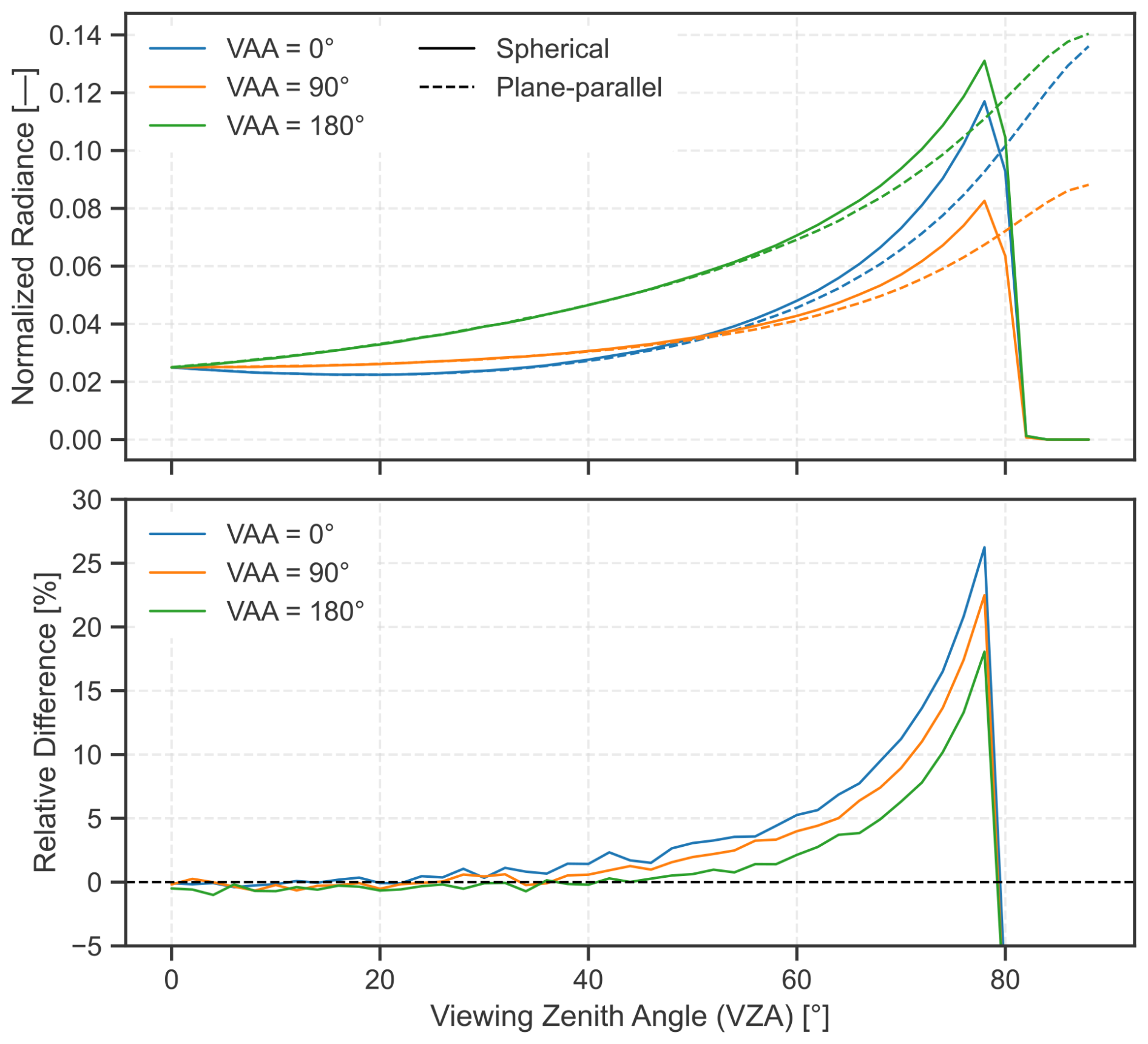
Figure 12 Comparison between spherical and plane-parallel geometry for a sensor at the top of the atmosphere. Line colours map to different viewing azimuth angles (VAAs). The solid lines show the results for spherical geometry, and the dashed lines those for plane-parallel geometry. The solar zenith angle is set to 60°.

8.1.4 Reflectance calculations

Eradiate can be used to compute reflectance quantities useful for EO applications. We follow the standard nomenclature established by Nicodemus et al. (1977) in the following. It should be noted that Eradiate computes only radiances, fluxes and powers, which means that reflectance quantities emerge after processing simulation results in a way similar to what would be done with experimental data: accessing some of the terms defined by Nicodemus et al. (1977) may require a specific simulation setup or an indirect computation.

The example notebook¹⁰ provided in the companion repository demonstrates how to compute:

• the “top of canopy” (TOC) BRF, obtained by computing the reflected radiance over a surface with no atmosphere, at the surface level;

• the “top of atmosphere” (TOA) BRF, obtained by computing the reflected radiance over a surface with an atmosphere, at the TOA level;

• the “bottom of atmosphere” (BOA) hemispherical directional reflectance factor (HDRF), obtained by combining the reflected radiance and incident radiant flux over a surface with an atmosphere, at the surface level.

Figure 13 shows that, even in a clear-sky scenario (i.e. without aerosols), the three quantities differ significantly. This can have significant impact: for instance, drones are now often used to measure the BOA hemispherical conical reflectance factor (HCRF), which is close to the BOA HDRF, and is identified to the TOC BRF. From a radiometric point of view, this is not correct; however, if one can tolerate a certain level of inaccuracy, quantified by Schunke et al. (2023), the BOA HCRF can be used as a TOC BRF.

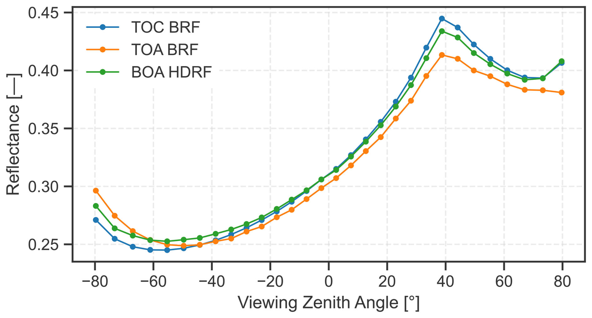
Figure 13 The TOA BRF (surface and atmosphere, sensor at satellite altitude), BOA HDRF (surface and atmosphere, sensor at top of canopy altitude) and TOC BRF (surface only, sensor at top of canopy altitude) for a retro-reflective RPV surface illuminated with a solar zenith angle of 38°. In the scenarios that include an atmosphere, a clear-sky AFGL 1986 (US Standard) profile is used. The values shown are computed using Eradiate in monochromatic at 550 nm.

8.1.5 Irradiance calculation

Irradiance is defined as the electromagnetic energy incident on a surface per unit time and per unit area. In Eradiate, irradiance can be computed using the distant_flux measure.

The example notebook¹¹ illustrates the simulation of diffuse and direct downwelling irradiances at the surface, as well as the upwelling irradiance reflected by the surface. The setup includes the US Standard atmosphere and a desert aerosol model (govaerts_2021_desert) designed to support the RAMI4ATM benchmarking exercise.¹² Irradiances are evaluated for varying AOTs and surface albedos.

Figure 14 shows the expected behaviour: as the AOT increases, more radiation is scattered within the atmosphere. This enhances the diffuse irradiance while reducing the direct irradiance. Increasing the surface albedo primarily raises the upwelling irradiance and, to some extent, the diffuse downwelling irradiance, since part of the reflected radiation is redirected back towards the surface. The direct irradiance, by contrast, represents unscattered radiation reaching the surface and is therefore unaffected by surface albedo.

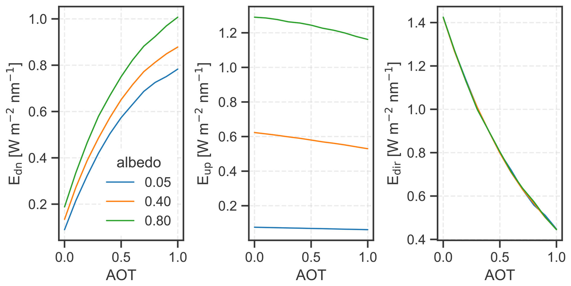
Figure 14 Simulated surface irradiances as functions of AOT and surface albedo. Shown are (left) diffuse downwelling irradiance E_dn, (middle) diffuse upwelling irradiance E_up, and (right) direct downwelling irradiance E_dir.

8.2 3D simulation

This series of examples showcase Eradiate's 3D surface simulation features with gradually increasing complexity in terms of required knowledge of Eradiate's expert interface.

8.2.1 Vegetated canopies from RAMI-V

This example shows how to use the automatic RAMI canopy loader, with or without padding the canopy with clones of itself, and with default or customized optical properties. The example notebook¹³ mainly uses perspective cameras for educational purposes, but the resulting scenes can be used readily to compute other quantities such as the ones defined in Sect. 8.1.4 (see Fig. 15). This setup is also used to create Fig. 3.

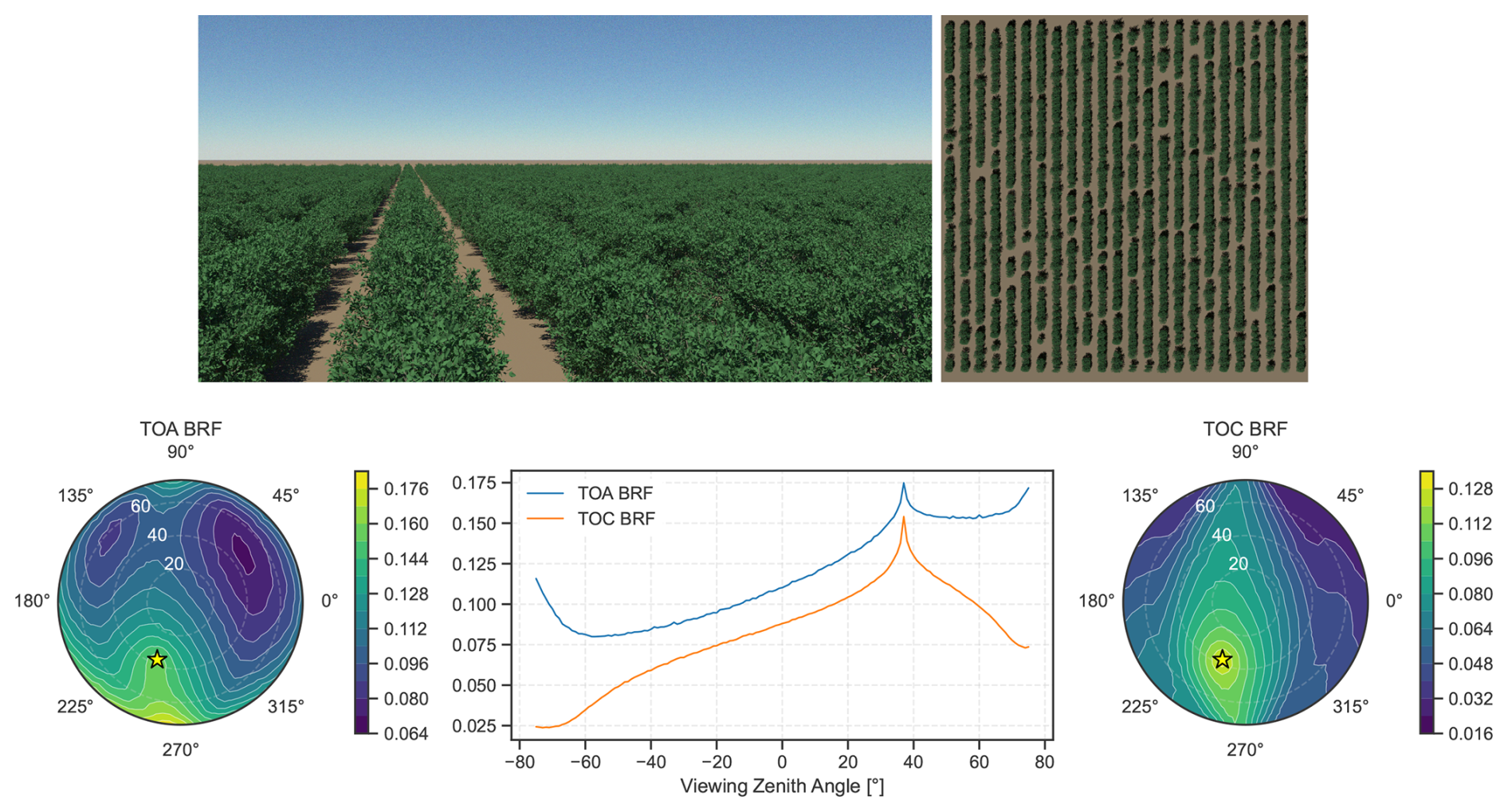
Figure 15 An example of output achievable with Eradiate's RAMI canopy loader. The scene is the Wellington Citrus Orchard (Stuckens et al., 2009; Somers et al., 2009). Top row: A perspective camera view of the scene (left), and a nadir-looking render of the unit cell (right). Bottom row: TOA (left) and TOC (right) reflectance of the Wellington Citrus Orchard scene. Both in the principal plane (centre). The TOA setup includes a clear-sky atmosphere (AFGL 1986 US Standard profile). Polar plots display the illumination direction with a star marker.

The highly directional features of the scene shown in Fig. 15 result in strong anisotropy in the canopy's reflective pattern, first at the TOC, and also at the TOA, showing a typical example where accounting for 3D surface features makes a significant difference when simulating satellite observations.

8.2.2 Algeria-5 pseudo-invariant calibration site

This example¹⁴ demonstrates a relatively simple use case of Eradiate's expert interface. It combines a spherical-shell background atmosphere (AFGL 1986 US Standard molecular atmosphere and an aerosol layer with an exponential vertical density distribution) with a triangulated DEM of the Algeria-5 PICS integrated directly as a Mitsuba primitive. This setup is used to create Fig. 2.

Topography is part of the complex 3D surface features that can cause deviations from the usual flat surface assumption mentioned in Sect. 1, e.g. when simulating satellite images above bright desert PICS, as illustrated by Govaerts (2015).

8.2.3 Sunset on Dakar

This last example is derived from a study in which a scene generator was implemented on top of the expert interface to create synthetic scenes derived from actual locations on Earth. In these scenes, a 100 km-sized area is divided into 100 m tiles populated with 3D geometry. Tiles are categorized based on a land cover map, and each type is assigned a set of 3D shapes and a background reflection model. These scenes exploit two important features:

• Instancing: The 3D shapes associated to a land cover type are loaded only once, then clone at every location where the land cover type is detected. In practice, this means that the geometry corresponding to the land cover type is loaded only once, which drastically reduces the memory footprint of the scene.

• Land cover-based material dispatching (see also Sect. 4.1.3): The background BRDFs of all land cover types are loaded into an index, which is then mapped spatially by a texture encoding the material with an 8-bit integer. This compact representation allows to map many reflection models with a high spatial resolution at a very low memory cost.

The output (see Fig. 16) shows an example of a coastal area near the city of Dakar, with both an in situ render and a synthetic satellite image. A similar setup is used to create Fig. 5.

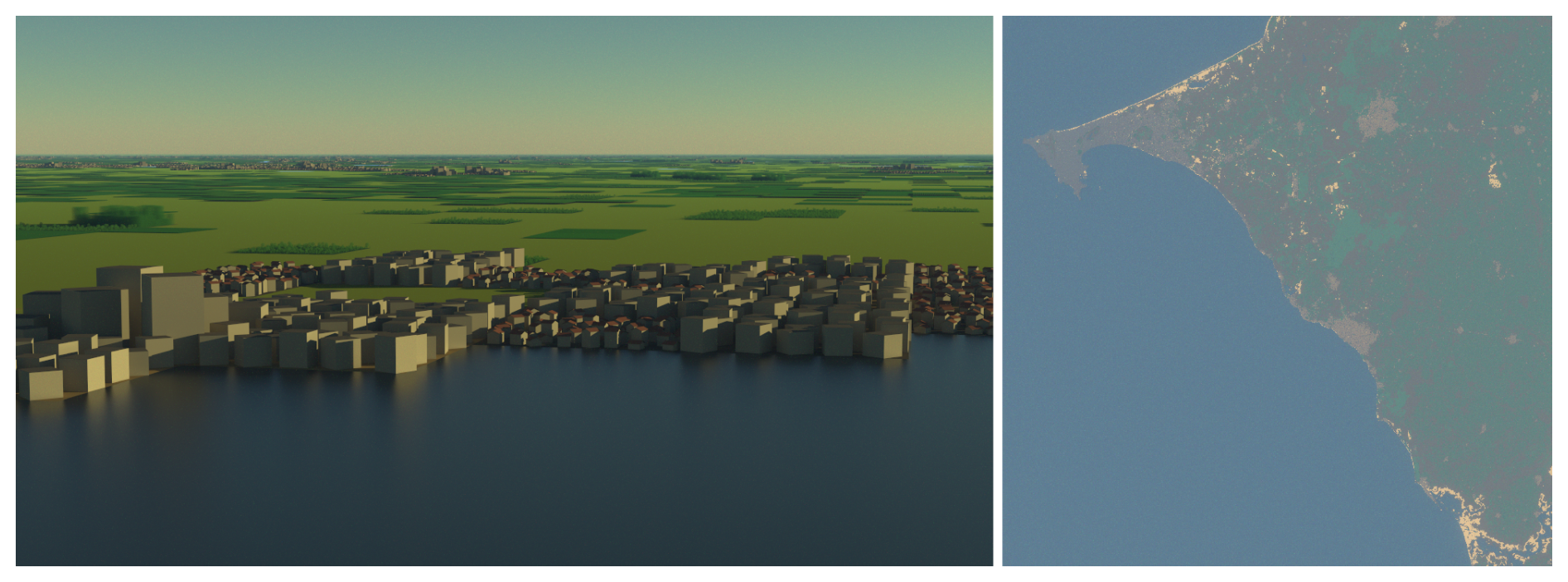
Figure 16 This synthetic scene is modelled after 100 km-wide area near the city of Dakar and created with a scene generator that leverages land cover information to select materials and clone instances of urban and vegetation 3D tiles. Except for the illumination angle, the RGB render (left) and the nadir-looking ortho-image (right) use identical scene input (land cover, a plane-parallel atmosphere with an AFGL 1986 US Standard profile and an aerosol layer with exponential density). The simulated pixel size of the ortho-image is 1 km, and the land cover tile size is 100 m.

This setup showcases the potential of Eradiate to simulate large scenes sourced from remote sensing data, with sensors at satellite level, and resolving metre-sized geometric features in a 100 km-sized area. The size of the scene and number of objects are such that they can be handled only thanks to features offered by the radiometric kernel, which demonstrates some of the many benefits brought by repurposing rendering software.

9 Conclusions and outlook

Eradiate builds on the history of radiative transfer simulation software for EO and incorporates modelling and technical advances made in other scientific fields, in particular computer graphics. The Mitsuba 3 renderer, integrated as our radiometric kernel, drastically simplifies the development of additional components, allows for providing a convenient Python-based interface and provides promising opportunities for future iterations of the model thanks to its retargetable architecture.

Eradiate v1.0.0 focuses on providing advanced surface modelling and 1D atmospheric modelling to meet the accuracy requirements for the vicarious calibration of modern instruments. The development roadmap includes the addition of 3D atmospheric scattering, as well as cloud-focused variance reduction techniques and optimizations to improve the efficiency of the MCRT algorithm. Extensions to the thermal infrared and microwave domains are planned. Finally, the simulation of volumetric scattering in aquatic bodies is foreseen. Continued validation, through regression detection against prior validated solutions, as well as benchmark participation, is planned.

A topic that was not explored so far by Eradiate is differentiable rendering. Mitsuba 3, and its underlying computational core Dr.Jit, have built-in infrastructure to differentiate simulations automatically, allowing to output gradients of a primal Monte Carlo estimator with respect to any variable in the scene (Jakob et al., 2022b). The simulation can then be included in an optimization loop to solve inverse problems. Inverse 3D radiative transfer problems in EO are extremely complex and still require a large amount of research for differentiable rendering techniques to be effective in that context; Eradiate has potential to contribute to that effort.

Eradiate is free software, intended to be both an easy entry point for radiative transfer beginners, a powerful tool allowing experts to build simulations with total freedom, and a sandbox for developers willing to experiment with new models, algorithms or scene setups, as illustrated by the examples shown in this paper. It hopefully contributes to making radiative transfer simulation software more comprehensive and accessible.

Appendix A: ROMC results examples in DEBUG mode

ROMC's DEBUG mode offers a broader scene variety than the VALIDATE mode and is an excellent testing sandbox for RTM development. Although the results submitted in this mode cannot be used to make claims on RTM performance, we show examples in Table A1 to illustrate the variety of surfaces that can be simulated with Eradiate.

Table A1 Examples of ROMC submissions in DEBUG mode.

Appendix B: General requirements

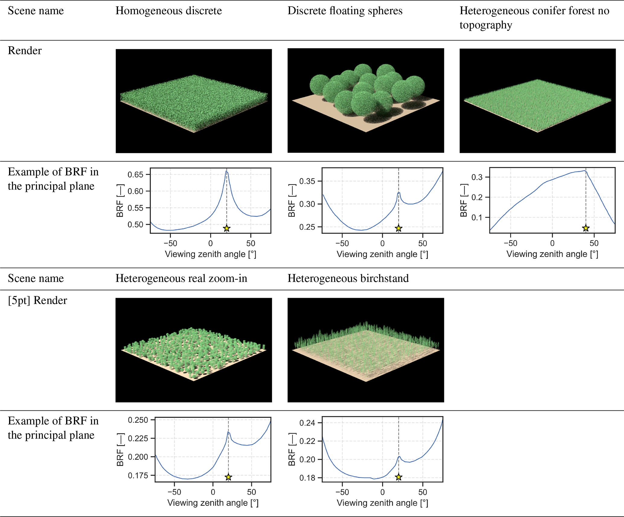
This appendix reviews the broad requirements which drive Eradiate's design. This is not a detailed requirement list, but it motivates some of the architectural and technological choices and numerical method selection decisions mentioned throughout this paper.

High accuracy. Eradiate primarily targets cal/val applications, with the ambition of eventually simulating satellite images with an accuracy better than 1 %, as mentioned in Sect. 1. This goal has consequences on the requirements underlying its design:

• Accuracy over performance. Since accuracy is the highest priority, it must not be sacrificed for performance. This means, in particular, that when selecting models and numerical methods, the candidate meeting the best Eradiate's accuracy requirements is prioritized, even if it is not the choice optimizing computational cost. This, however, does not mean that Eradiate's performance should not be optimized.

• 3D geometry support. High accuracy requires the support of 3D geometry to overcome the fundamental limitations of 1D models (“smooth and flat planet”). Here, 3D geometry is to be understood in a broad sense, and covers planetary curvature, terrain modelling, cloud modelling, non-uniform surface reflective properties and explicit surface geometric representation (detailed trees and buildings).

• Monte Carlo ray tracing. The very high scene complexity implied by the handling of 3D geometry features makes MCRT the natural method of choice to solve the RTE. MCRT can indeed deal with arbitrarily complex problems and solve them efficiently if correctly implemented. MCRT also has the big advantage of handling arbitrary length-scale complexity, making it possible, in principle, to include, in a fully coupled simulation, both centimetre- and kilometre-sized objects.

• State-of-the-art molecular absorption. We saw that molecular absorption modelling is a source of disagreement between RTMs and is also the cause of inaccuracies in satellite bands where it plays a significant role. Eradiate should implement state-of-the-art molecular absorption models, which starts with the ubiquitous CKD distribution method. It should be noted that the input data is as critical as the numerical method: Eradiate also has to ship high-quality atmospheric data.

Traceability and reliability. Traceability refers to the possibility to know where algorithms and data come from. This is an essential quality for a product meant for cal/val applications, but also for a community-oriented project. Reliability is the possibility to understand how well the software will achieve tasks executed with it. Eradiate covers these topics as follows:

• Free and open-source software. Eradiate is licensed under the GNU Lesser General Public License (LGPLv3) and designed as free software. Its source code is freely available and can be studied and audited.

• Extensive algorithm and data documentation. Eradiate ships with extensive documentation, with a user manual, tutorials and complete code reference. Data is self-documented using metadata.

• Benchmarking. Regular comparison exercises, based on benchmarks, are conducted. This way, we verify that the results produced by Eradiate are in line with other models in relevant situations.

Modern technology. This project was started with the intention of making radiative transfer modelling more accessible to users and developers.

• Modular architecture. Eradiate is designed in a modular way, using abstractions inspired by the architecture of the rendering software and incorporating EO idioms. This facilitates code maintenance, but also makes it possible to change parts of the model with only partial knowledge of how it works.

• Robust testing process. The codebase is systematically tested using pytest (Krekel et al., 2004). The test suite includes unit tests checking basic functionality, but also larger integration tests verifying that the model always performs consistently. In particular, selected benchmarking cases are used for regression testing.

• User-friendly Python interface. A typical scientific workflow often involves using software through an interactive Python console such as a Jupyter notebook (Kluyver et al., 2016). Eradiate is designed to address such use cases well and makes it easy to define and inspect simulations, run computations, and visualize results interactively.

Appendix C: User interface

Eradiate's user interface relies entirely on Python programming. Various features are implemented to make configuration code less error-prone, briefer and more enjoyable to write:

Algorithm C1 Basic interface.

1:

import numpy as np

2:

import eradiate

3:

from eradiate.experiments import AtmosphereExperiment

4:

from eradiate.scenes.atmosphere import MolecularAtmosphere

5:

from eradiate.scenes.bsdfs import LambertianBSDF

6:

from eradiate.scenes.measure import MultiDistantMeasure

7:

from eradiate.scenes.illumination import DirectionalIllumination

8:

9:

# Select mode before doing anything else

10:

eradiate.set_mode(“ckd”)

11:

12:

# Configure the experiment

13:

exp = AtmosphereExperiment(

14:

atmosphere=MolecularAtmosphere(),

15:

surface=LambertianBSDF(reflectance=0.5),

16:

illumination=DirectionalIllumination(azimuth=45.0, zenith=30.0),

17:

measures=MultiDistantMeasure.hplane(azimuth=45.0, zeniths=np.arange(-75, 76, 5.0)),

18:

)

19:

20:

# Run the simulation

21:

# The `spp' parameter controls the number of Monte Carlo samples at each

22:

# iteration of the spectral loop

23:

result = eradiate.run(exp, spp=10000)

24:

25:

# Display the results using xarray's plotting features

26:

result[”brf”].plot()

Algorithm C2 Basic interface (dictionary-based).

1:

import numpy as np

2:

import eradiate

3:

from eradiate.experiments import AtmosphereExperiment

4:

5:

eradiate.set_mode(”ckd”)

6:

7:

exp = AtmosphereExperiment(

8:

atmosphere={”type”: ”molecular”},

9:

surface={”type”: ”lambertian”},

10:

illumination={”type”: ”directional”, ”azimuth”: 45.0, ”zenith”: 30.0},

11:

measures={

12:

”type”: ”mdistant”,

13:

”construct”: ”hplane”,

14:

”azimuth”: 45.0,

15:

”zeniths”: np.arange(-75, 76, 5.0),

16:

},

17:

)

18:

19:

result = eradiate.run(exp, spp=10000)

20:

21:

result[”brf”].plot()

Algorithm C3 Expert interface.

1:

import mitsuba as mi

2:

3:

import eradiate

4:

from eradiate import KernelContext

5:

from eradiate import unit_registry as ureg

6:

from eradiate.kernel import scene_parameter

7:

8:

eradiate.set_mode(”mono”)

9:

10:

11:

# Define ”yellow” reflectance spectrum

12:

VALUES = {440.0: 0.1, 550.0: 0.5, 660.0: 0.9}

13:

14:

def spectrum_lambertian(ctx: KernelContext):

15:

return VALUES[ctx.si.w.m_as(”nm”)]

16:

17:

18:

# Declare an Experiment with custom kernel dictionary and parameters

19:

exp = eradiate.experiments.AtmosphereExperiment(

20:

atmosphere={”type”: ”molecular”},

21:

surface={”type”: ”lambertian”},

22:

measures={

23:

”type”: ”perspective”,

24:

”origin”: [5, 5, 1],

25:

”target”: [0, 0, 0.5],

26:

”film_resolution”: (320, 240),

27:

”srf”: {”type”: ”delta”, ”wavelengths”: [440, 550, 660]},

28:

},

29:

kdict={

30:

”mat_thesphere”: {”type”: ”diffuse”, ”id”: ”mat_thesphere”},

31:

”mat_thesquare”: {”type”: ”roughplastic”, ”id”: ”mat_thesquare”},

32:

”sphere”: {

33:

”type”: ”sphere”,

34:

”id”: ”thesphere”,

35:

”bsdf”: {”type”: ”ref”, ”id”: ”mat_thesphere”},

36:

},

37:

”square”: {

38:

”type”: ”rectangle”,

39:

”to_world”: mi.ScalarTransform4f.translate([0, 0, 0.1])

40:

@ mi.ScalarTransform4f.scale(2.0),

41:

”bsdf”: {”type”: ”ref”, ”id”: ”mat_thesquare”},

42:

},

43:

},

44:

kpmap={

45:

”mat_thesphere.reflectance.value”: scene_parameter(

46:

spectrum_lambertian,

47:

node_type=mi.BSDF,

48:

node_id=”mat_thesphere”,

49:

parameter_relpath=”reflectance.value”,

50:

),

51:

},

52:

)

53:

54:

55:

# Run simulation

56:

result = eradiate.run(exp, spp=256)

• Unit handling. Whenever relevant, numeric quantities handled by Eradiate are attached physical units using the Pint library (Grecco, 2022). This enforces dimensional consistency and guarantees unit conversion when relevant. This lets users input their data in the set of units they are most familiar with and makes using Eradiate easier for users unfamiliar with domain-specific units. To reduce input verbosity, values provided without units are automatically converted to configurable default units.

• Data delivery and consumption. Eradiate comes with various data (e.g. absorption cross-section databases, sensor spectral response, aerosol single-scattering properties) managed by an asset manager which, in practice, behaves like a basic package manager with a command-line interface. When consuming data, relative filesystem paths are resolved according to a configurable list of locations, which allows relocating data without modifying any code.

• Object attribute pre-processing. Eradiate uses the attrs library (Schlawack, 2024) to implement object initialization sequences. A range of converters and validators can pre-process values used to initialize scene element objects and check if their attributes have correct values. Failed validations raise exceptions which can be tracked to the code that emitted them using the Python traceback.

Example: Basic interface. Algorithm C1 shows a basic configuration for a 1D atmospheric radiative transfer simulation that outputs the TOA BRF of the scene in the principal plane.

All scene elements can also be instantiated from basic Python dictionaries. An Experiment can therefore be initialized either using Python objects explicitly, or using a dictionary in the style of the Mitsuba dictionary-based scene specification. This input method is preferred for its conciseness. Algorithm C2 refactors algorithm C1 with this approach.

Example: Expert interface. Algorithm C3 shows an example of complex scene building using the expert interface. Of notable importance is the need to hint Eradiate when searching the Mitsuba scene parameters which will undergo updates during the spectral loop using the keyword arguments of the scene_parameter() function.

Appendix D: List of the main acronyms

AOT	aerosol optical thickness
BOA	bottom of atmosphere
BRF	bidirectional reflectance factor
BRDF	bidirectional reflectance distribution function
BSDF	bidirectional scattering distribution function
BVH	bounding volume hierarchy
CKD	correlated-k distribution
CAMS	Copernicus atmosphere monitoring service
DEM	digital elevation model
EO	Earth observation
HDRF	hemispherical directional reflectance factor
MCRT	Monte Carlo ray tracing
PICS	pseudo-invariant calibration site
TOA	top of atmosphere
TOC	top of canopy
RTLS	RossThick-LiSparse
RTM	radiative transfer model
RTE	radiative transfer equation
RPV	Rahman-Pinty-Verstraete
SRF	spectral response function
VAA	viewing azimuth angle
VZA	viewing zenith angle
VRTE	vector radiative transfer equation