Implementation and evaluation of sea level operators in OceanVar2.0: an open-source oceanographic three-dimensional variational data assimilation system

This study presents the development and sensitivity analysis of the sea level operator within the OceanVar software which implements an oceanographic incremental three-dimensional variational data assimilation scheme. In OceanVar, the background error covariance matrix is decomposed into a sequence of physically based linear operators, allowing for individual analysis of specific error matrix components. The key development of OceanVar2.0 is the full integration of both dynamic height and barotropic model formulations as a flexible option for handling sea level covariance. The comparison of the two formulations of the sea level operator which provides correlations between Sea Level Anomaly, temperature and salinity increments is presented. The sensitivity experiments were performed in the Mediterranean Sea and the quality of the analysis assessed by comparing background estimates with observations for the period January–December 2021. The results confirm the methodological advantage of the barotropic model operator, which successfully overcomes the physical and operational limitations associated with choosing an appropriate level-of-no-motion for the dynamic height formulation. Furthermore, we present a method to assimilate along-track satellite altimetry considering a forecasting model with tides.

1 Introduction

Understanding the past state of the ocean and predicting its future behaviour is critical for sustainable development and for climate change mitigation and adaptation strategies. Oceans are a key component of the Earth's climate system, and they require specific data assimilation schemes due to the sparsity of data in the ocean interior. There are different methodologies for ocean data assimilation, each with its own strengths and weaknesses. Within inverse problem theory, the two most used approaches are the variational and the Kalman filter (Carrassi et al., 2018). Schemes based on Monte-Carlo algorithms, such as the Particle filter, have been proven to be successful on low-dimensional systems and have become feasible for high-dimensional geophysical systems only recently (Van Leeuwen et al., 2019). The choice of data assimilation method depends on factors such as the type of the observations, the desired forecast horizon, and the available computational resources.

Recent machine learning (ML) advancements offer potential optimizations for ocean data assimilation (e.g., Barthélémy et al., 2022; Beauchamp et al., 2023). ML can refine the representation of the errors and reveal complex relationships, improving accuracy. To fully leverage ML and new data streams, modular and flexible data assimilation software is essential. As research progresses, these advancements will significantly enhance our ability to understand and predict ocean behaviour.

The data assimilation community has made substantial strides in developing widely used software tools and specific implementations. General frameworks such as PDAF (Nerger and Hiller, 2013) and DART (Data Assimilation Research Testbed, Anderson et al., 2009) have contributed significantly to the field. Additionally, model-specific implementations such as ROMS-4DVAR (Moore et al., 2011) have been instrumental in advancing ocean data assimilation. Each of these tools offers unique capabilities, and the increasing complexity of data assimilation problems – particularly with the adoption of ML – drives the continuous development and innovation of both existing and new tools in the community, as evidenced by recent research (Martin et al., 2025).

OceanVar is the data assimilation software used in this study. It was first introduced by Dobricic and Pinardi (2008, hereafter DP08) and implements an incremental three-dimensional variational method. OceanVar features a modular design that allows for flexibility in incorporating diverse data sources and error covariance representations. This adaptability has made it suitable for a wide range of applications and research needs. The software has been extensively used in several operational and reanalysis systems, as evidenced by numerous publications (Dobricic et al., 2007; Storto et al., 2016; Escudier et al., 2021; Lima et al., 2021; Ciliberti et al., 2022; Coppini et al., 2023). It has been used to test new hybrid formulations (Oddo et al., 2016; Storto et al., 2018) and to implement new observational operators for different data types, including Lagrangian trajectories (Nilsson et al., 2012), sea-ice variables (Cipollone et al., 2023), daytime SST from SEVIRI (Storto and Oddo, 2019), and AI-based operators (Storto et al., 2021; Broccoli and Cipollone, 2025). Furthermore, it has been instrumental in improving error covariance models (Dobricic et al., 2015) and advancing specific applications, such as biogeochemical modelling (Teruzzi et al., 2014, 2018), and new interdisciplinary uses like assessing the impact on underwater acoustic predictions (Storto et al., 2020).

The extensive use of the code in diverse applications has led to the creation of different versions, some of which are inconsistent or incompatible. This core issue drives the development presented here. For this study, we used OceanVar2.0 (hereafter OceanVar2 for improved readability), a new version of the underlying OceanVar framework that unifies the various developments into a single, consistent, and fully parallelized software package.

In DP08 and all subsequent developments, horizontal covariance was approximated using the recursive filter (Lorenc, 1992; Hayden and Purser, 1995). The filter is conceptually simple, typically requiring only a few iterations to approximate the Gaussian function, and its application on a horizontal grid can be split into two independent directions (Purser et al., 2003). However, in cases of spatially or temporally varying correlation radii, the computational advantage of the recursive filter may be questioned (Purser et al., 2022). To provide the system with greater flexibility in terms of horizontal correlation radii, OceanVar2 models the horizontal correlation by a repeated application of the Laplacian operator, which is also the solution of the horizontal diffusion equation (e.g., Derber and Rosati, 1989; Weaver and Courtier, 2001).

Satellite altimetry and satellite-derived sea surface temperature are crucial in bridging gaps left by in-situ observations (Le Traon et al., 2025). Satellites help to cover almost the entire ocean surface and satellite altimetry contains information of the subsurface thermohaline structure that is key to obtain best estimates of the ocean variability at depth. Satellite altimetric sea level data are available from 1992, and altimeters have increased in coverage in the past ten years. The effective integration of satellite altimetry and sea surface temperature data into model corrections requires advanced extrapolation algorithms. While this necessity was first emphasized in foundational work (De Mey and Robinson, 1987), it continues to drive development in the field, as evidenced by cutting-edge solutions using machine learning (Zavala-Romero et al., 2025). In this work we demonstrate the capability of OceanVar2 to effectively assimilate along-track satellite altimetry with the use of a barotropic model operator and multivariate sea level, temperature and salinity statistics. Although the barotropic model was conceptually defined in DP08, its implementation was not carried forward or maintained in subsequent mainline versions. This work presents its full integration and optimization within the OceanVar2 framework. We present, for the first time, a detailed, direct comparison of the barotropic model defined by DP08 with the dynamic height operator. Additionally, OceanVar2 is applied to the latest version of the Mediterranean Sea forecasting System (Clementi et al., 2023) that considers tidal forcing. Tides are becoming an essential component of the resolved variability of the ocean general circulation, and they can no longer be neglected in numerical ocean circulation models (Arbic, 2022). Satellite altimeters sample tides along their track as well as the mesoscales. Using OceanVar2 we present a preliminary solution to the problem of assimilation in presence of tidal components both in model and observations.

The manuscript is organized as follows. After the introduction, Sect. 2 provides a general overview of the variational formulation and the characteristics of OceanVar2. Section 3 presents the background and the observational error covariance matrix formulation and their specific operators. Section 4 describes the experimental setup and the altimetry assimilation methods. Section 5 discusses the results. Section 6 provides an overview of the computational performance of the code. Finally, Sect. 7 provides the summary and conclusions.

2 Formulation of the Variational Assimilation Scheme

The standard cost function in three-dimensional variational data assimilation is defined as:

$$\begin{array}{}\text{(1)}& \begin{array}{rl}J\left(\mathit{x}\right)& ={\displaystyle \frac{\mathrm{1}}{\mathrm{2}}}{\left(\mathit{x}-{\mathit{x}}_{\mathrm{b}}\right)}^{\mathrm{T}}{\mathbf{B}}^{-\mathrm{1}}\left(\mathit{x}-{\mathit{x}}_{\mathrm{b}}\right)\\ & +{\displaystyle \frac{\mathrm{1}}{\mathrm{2}}}{\left(\mathit{y}-\mathit{h}\left[\mathit{x}\right]\right)}^{\mathrm{T}}{\mathbf{R}}^{-\mathrm{1}}\left(\mathit{y}-\mathit{h}\left[\mathit{x}\right]\right)\end{array}\end{array}$$

where, x is the analysis state vector containing the ocean model prognostic variables, x_b is the background state vector, B is the background error covariance matrix, h is the non-linear observational operator, y are the observations, R is the observational error covariance matrix and T indicates the matrix transpose. Equation (1) is linearized around the background state (e.g., Lorenc, 1997) and expressed in terms of the increments $\mathit{\delta }\mathit{x}=\mathit{x}-{\mathit{x}}_{\mathrm{b}}$:

$$\begin{array}{}\text{(2)}& J\left(\mathit{\delta }\mathit{x}\right)={\displaystyle \frac{\mathrm{1}}{\mathrm{2}}}\mathit{\delta }{\mathit{x}}^{\mathrm{T}}{\mathbf{B}}^{-\mathrm{1}}\mathit{\delta }\mathit{x}+{\displaystyle \frac{\mathrm{1}}{\mathrm{2}}}{\left(\mathit{d}-\mathbf{H}\mathit{\delta }\mathit{x}\right)}^{\mathrm{T}}{\mathbf{R}}^{-\mathrm{1}}\left(\mathit{d}-\mathbf{H}\mathit{\delta }\mathit{x}\right),\end{array}$$

where $\mathit{d}=\mathit{y}-\mathit{h}\left[{\mathit{x}}_{\mathrm{b}}\right]$ are the misfits (or innovations), and H is the Jacobian matrix of h at x=x_b. The analysis at a particular time is defined as ${\mathit{x}}_{\mathrm{a}}={\mathit{x}}_{\mathrm{b}}+\mathit{\delta }\mathit{x}$, where J attains its minimum.

Existence and uniqueness of x_a is guaranteed because J is quadratic with R and B positive definite matrices. The minimum can be found by forcing the gradient of the cost function to zero. The gradient of Eq. (2) is:

$$\mathrm{\nabla }J\left(\mathit{\delta }\mathit{x}\right)=\left({\mathbf{B}}^{-\mathrm{1}}+{\mathbf{H}}^{\mathrm{T}}{\mathbf{R}}^{-\mathrm{1}}\mathbf{H}\right)\mathit{\delta }\mathit{x}-{\mathbf{H}}^{\mathrm{T}}{\mathbf{R}}^{-\mathrm{1}}\mathit{d}$$

Following DP08, the OceanVar scheme assumes that the B matrix can be decomposed as:

$$\mathbf{B}={\mathbf{VV}}^{\mathrm{T}}$$

and the cost function may equivalently be minimized using a new control variable v (e.g., Lorenc, 1997) defined using the transformation matrix V⁺:

$$\mathit{v}={\mathbf{V}}^{+}\mathit{\delta }\mathit{x},$$

where the superscript “+” indicates the generalized inverse. The vector v is defined on the control space, and the increment vector δx on the physical space. The cost function (2) now obtains the form:

$$J\left(\mathit{v}\right)={\displaystyle \frac{\mathrm{1}}{\mathrm{2}}}{\mathit{v}}^{\mathrm{T}}\mathit{v}+{\displaystyle \frac{\mathrm{1}}{\mathrm{2}}}{\left(\mathbf{HV}\mathit{v}-\mathit{d}\right)}^{\mathrm{T}}{\mathbf{R}}^{-\mathrm{1}}\left(\mathbf{HV}\mathit{v}-\mathit{d}\right).$$

The misfit in OceanVar is estimated using the FGAT (First Guess at Appropriate Time) method. The valid time of the increment using the FGAT algorithm has been discussed and investigated in literature (see Massart et al., 2010). The purpose of FGAT is to ensure that each observation (y_i) falling within the assimilation window [$t_n;t_{n+\mathrm{1}}$] is compared against the model background (x_b) at the specific time of the observation (t_i), rather than only at the final analysis time (t_n+1). The innovations (d_i) are thus computed as:

$$d_{\mathrm{i}}=\left({\mathit{y}}_{\mathrm{i}}-\mathit{h}\left[{\mathit{x}}_{\mathrm{b}}\left(t_i\right)\right]\right),$$

where x_b(t_i) is the model background interpolated to the observational time t_i. The assimilation system then minimizes all these innovations to compute a single analysis increment (δx) which is applied at t_n+1. Formally our analysis is defined as the instantaneous field:

$${\mathit{x}}_{\mathrm{a}}\left(t_{n+\mathrm{1}}\right)={\mathit{x}}_{\mathrm{b}}\left(t_{n+\mathrm{1}}\right)+\mathit{\delta }x,$$

where x_b(t_n+1) is the instantaneous background field simulated by the nonlinear ocean model starting from t_n.

3 Modelling the background error covariance matrix

The transformation matrix V is modelled at each minimization iteration as a sequence of linear operators (e.g., Weaver et al., 2003). In this way, V successively transforms increments in the control space towards final increments in the physical space.

In OceanVar and OceanVar2 the matrix V is defined in the following way:

$$\begin{array}{}\text{(3)}& \mathbf{V}={\mathbf{V}}_{\mathrm{D}}{\mathbf{V}}_{u,v}{\mathbf{V}}_{\mathit{\eta }}{\mathbf{V}}_{\mathrm{H}}{\mathbf{V}}_{\mathrm{V}}\end{array}$$

From right to left, V_V defines the vertical error covariance; V_H the horizontal error correlation; V_η is the sea level operator containing correlation between temperature, salinity and sea surface elevation; and V_u,v forces a geostrophic balance between temperature, salinity and the velocity components. Finally, V_D is a divergence-damping operator avoiding spurious currents close to the coast in the presence of complex coastlines, as defined by DP08.

The vertical transformation operator V_V has the form:

$${\mathbf{V}}_{\mathrm{V}}={\mathbf{S}}_{\mathrm{c}}{\mathbf{\Lambda }}_{\mathrm{c}}^{\mathrm{1}/\mathrm{2}}$$

where columns of S_c contain eigenvectors and Λ_c is a diagonal matrix with eigenvalues of multivariate Empirical Orthogonal Functions (EOFs). In the OceanVar and OceanVar2 code, the EOFs can be defined pointwise (Coppini et al., 2023) or by regions (DP08).

Differently from DP08, to account for horizontal correlations, V_H is considered as the discretized form of the diffusive operator:

$${\mathbf{V}}_{\mathrm{H}}={\mathbf{\nabla }}_{\mathrm{H}}\cdot \left(k_{\mathrm{c}}{\mathbf{\nabla }}_{\mathrm{H}}C\right)$$

where ∇_H is the horizontal differential operator, k_c is the spatially variable diffusivity coefficient corresponding to horizontal correlation lengths, and C is a generic increment. Assuming a gaussian solution (Weaver and Courtier, 2001), the relation between k_c and the horizontal correlation radius is:

$$R_{\mathrm{H}}=\sqrt{\mathrm{2}{k}_{\mathrm{c}}\mathrm{\Delta }t}$$

Where R_H, in meters, is the horizontal correlation radius, and Δt=1 s is the pseudo time-step used to integrate the diffusion equation. This filter was implemented using a dimensional splitting approach. The operator is discretized with a Euler-Backward implicit scheme solved by means of LU decomposition of a tridiagonal matrix, following Hoffman and Frankel (2001). The tridiagonal matrix algorithm is chosen for its simplicity and the resulting ease of implementing its adjoint operator, its memory efficiency, and its ability to avoid external libraries implementing direct methods, thus forming a compact implementation which simplifies the porting of OceanVar2.

The V_η operator, the focus of this study, incorporates correlations between sea surface elevation and the subsurface thermohaline structure. Section 3.1 is dedicated to the detailed description of the two formulations implemented in OceanVar2.

The present formulation of OceanVar also allows for the computation of corrections for the velocity field: the V_u,v operator computes the velocity corrections assuming geostrophic balance. This assumption results in an operator with small computational cost. However, this assumption is not valid at the equator and may produce velocity vectors orthogonal to the coast. When imposing the zero-boundary condition for the velocity component perpendicular to the coast, the divergence component of the velocity field may become unrealistically large. Therefore, the divergence damping operator V_D in Eq. (3) is implemented to damp velocity divergence near coasts, while the vorticity remains unchanged. Details on the implementation of the divergence damping operator are provided in DP08.

As highlighted in DP08, the sequence of operator multiplication is critical and determined through a combination of physical reasoning and iterative experimentation. Initially, all increments are projected onto multivariate EOFs for sea level, temperature, and salinity, as these effectively capture ocean stratification (Sanchez de la Lama et al., 2016) and the relationship with sea level for assimilation purposes (De Mey and Robinson, 1987). Next, the increments are distributed horizontally. Following this, adjustments due to the sea level operator are computed based on the vertically projected temperature and salinity increments. Subsequently, increments in horizontal velocities are derived, and the process concludes with the application of the divergence damping filter.

3.1 The sea level operator and its relationship with the velocity terms

Dobricic et al. (2007) found that the vertical EOFs computed from the covariance between temperature, salinity and sea level could produce corrections that are not geostrophically balanced and proved that the enforcement of the geostrophic relationship for the sea level in the error covariance matrix has a significant positive impact on the accuracy of the analysis. Thus, in OceanVar2 the sea surface height increments from EOF projections are overwritten using a sea level operator. Two different sea level operators, with different levels of complexity, are implemented in OceanVar2.

The first is the commonly used Dynamic Height operator (V_η=V_DH), which is defined as:

$$\begin{array}{}\text{(4)}& {\mathbf{V}}_{\mathrm{DH}}=\mathit{\delta }{\mathit{\eta }}^{\mathrm{DH}}=-{\displaystyle \frac{\mathrm{1}}{{\mathit{\rho }}_{\mathrm{0}}}}\underset{-D}{\overset{\mathrm{0}}{\int }}\left[-\mathit{\alpha }\mathit{\delta }T+\mathit{\beta }\mathit{\delta }S\right]\mathrm{d}z\end{array}$$

Where D is a uniform reference level, corresponding to a level-of-no-motion, δT and δS are temperature and salinity increments respectively, α and β the expansion and contraction coefficients. The correlation between Sea Level Anomaly (SLA) from altimetry measurements and the dynamic height anomaly computed from in-situ measurements is high for regions deeper than 1000 m (Dhomps et al., 2011), at synoptic, seasonal and interannual time scales.

OceanVar2 allows the application of a more complex linear V_η. This operator is based on the formulation published in DP08 and derives from the steady state results of a linear barotropic model forced by buoyancy anomalies induced by the temperature and salinity increments. While the methodology was previously described in the literature, the barotropic model code itself was fully re-introduced and parallelized to function efficiently within the new OceanVar2 framework, with its general mathematical structure remaining unchanged. Its inclusion as a fully integrated option is a new feature of this version. The barotropic model equations, discretized in time by the semi-implicit scheme (Kwizak and Robert, 1971), are:

$$\begin{array}{}\text{(5)}& {\displaystyle }\begin{array}{rl}& {\displaystyle \frac{U^{n+\mathrm{1}}-U^{n-\mathrm{1}}}{\mathrm{2}\mathrm{\Delta }t}}-f{V}^n=\\ & -gH{\displaystyle \frac{\partial {\mathit{\eta }}^{\ast }}{\partial x}}-\underset{-H}{\overset{\mathrm{0}}{\int }}\left[\underset{-z}{\overset{\mathrm{0}}{\int }}{\displaystyle \frac{\partial \left(\mathit{\delta }b\right)}{\partial x}}\mathrm{d}{z}^{\prime }\right]\mathrm{d}z+\mathit{\gamma }{\mathrm{\nabla }}^{\mathrm{2}}{U}^{\ast }\end{array}\text{(6)}& {\displaystyle }\begin{array}{rl}& {\displaystyle \frac{V^{n+\mathrm{1}}-V^{n-\mathrm{1}}}{\mathrm{2}\mathrm{\Delta }t}}+f{U}^n=\\ & -gH{\displaystyle \frac{\partial {\mathit{\eta }}^{\ast }}{\partial y}}-\underset{-H}{\overset{\mathrm{0}}{\int }}\left[\underset{-z}{\overset{\mathrm{0}}{\int }}{\displaystyle \frac{\partial \left(\mathit{\delta }b\right)}{\partial y}}\mathrm{d}{z}^{\prime }\right]\mathrm{d}z+\mathit{\gamma }{\mathrm{\nabla }}^{\mathrm{2}}{V}^{\ast }\end{array}\end{array}$$

$${\displaystyle \frac{{\mathit{\eta }}^{n+\mathrm{1}}-{\mathit{\eta }}^{n-\mathrm{1}}}{\mathrm{2}\mathrm{\Delta }t}}+\left({\displaystyle \frac{\partial U^{\ast }}{\partial x}}+{\displaystyle \frac{\partial V^{\ast }}{\partial y}}\right)=\mathrm{0}$$

where U and V are vertically integrated velocity components, f is the Coriolis parameter, g is the acceleration due to gravity, H is the bottom depth, η is the surface elevation, δb is the buoyancy anomaly, and γ is the horizontal viscosity coefficient. The superscripts indicate the time step relative to n, and the superscript “*” indicates the weighted average between two timesteps. A more detailed description of the barotropic model and its discretization can be found in DP08. In the present version the barotropic model assumes closed lateral boundaries.

In the previous Eqs. (5) and (6), the buoyancy forcing term is defined as:

$$\mathit{\delta }b=g\left({\displaystyle \frac{\mathit{\delta }\mathit{\rho }}{{\mathit{\rho }}_{\mathrm{0}}}}\right)$$

and the density perturbation δρ is estimated by the linear equation of state:

$$\begin{array}{}\text{(7)}& \mathit{\delta }\mathit{\rho }=\mathit{\alpha }\mathit{\delta }T-\mathit{\beta }\mathit{\delta }S\end{array}$$

Expansion and contraction coefficients (α and β) in Eqs. (4) and (7) can be assumed space independent or spatially variable and estimated by linearizing the equation of state around a user defined background temperature (T_b) and salinity field (S_b):

$$\begin{array}{c}{\displaystyle }\mathit{\alpha }={\displaystyle \frac{\partial \mathit{\rho }}{\partial T}}{\mathrm{|}}_{T=T_{\mathrm{b}},S=S_{\mathrm{b}}}\\ {\displaystyle }\mathit{\beta }={\displaystyle \frac{\partial \mathit{\rho }}{\partial S}}{\mathrm{|}}_{T=T_{\mathrm{b}},S=S_{\mathrm{b}}}\end{array}$$

In the latter case the coefficients are read from an external input file.

In OceanVar2 the sea level operators produce the final sea surface height increments, replacing the increment produced by the cross-covariance between temperature, salinity and sea level provided by the EOFs (DP08, Storto et al., 2018).

The choice on the sea level operator has consequences on the velocity operator V_u,v. V_u,v computes the velocity correction assuming geostrophic balance under the Boussinesq and incompressibility approximations:

$$\begin{array}{c}{\displaystyle }f{u}_g\left(z\right)=-{\displaystyle \frac{\mathrm{1}}{{\mathit{\rho }}_{\mathrm{0}}}}{\displaystyle \frac{\partial p}{\partial y}}\\ {\displaystyle }f{v}_g\left(z\right)=+{\displaystyle \frac{\mathrm{1}}{{\mathit{\rho }}_{\mathrm{0}}}}{\displaystyle \frac{\partial p}{\partial x}}\end{array}$$

Decomposing the pressure p at any level z as:

$$p\left(z\right)=p_{\mathrm{atm}}+g{\mathit{\rho }}_{\mathrm{0}}\left(\mathit{\eta }+\underset{-z}{\overset{\mathrm{0}}{\int }}{\displaystyle \frac{\mathit{\delta }\mathit{\rho }}{{\mathit{\rho }}_{\mathrm{0}}}}\mathrm{d}z\right)$$

where p_atm is the atmospheric pressure, g is the effective gravity, η is the free surface elevation and δρ is the density departure from a reference state ρ₀. Neglecting the atmospheric pressure, and rewriting the hydrostatic term as buoyancy term, the geostrophic velocities become:

$$\begin{array}{}\text{(8)}& {\displaystyle }{\mathrm{fu}}_g\left(z\right)=-\left(g{\displaystyle \frac{\partial \mathit{\eta }}{\partial y}}+\underset{-z}{\overset{\mathrm{0}}{\int }}{\displaystyle \frac{\partial \mathit{\delta }b}{\partial y}}\mathrm{d}z\right)\text{(9)}& {\displaystyle }{\mathrm{fv}}_g\left(z\right)=+\left(g{\displaystyle \frac{\partial \mathit{\eta }}{\partial x}}+\underset{-z}{\overset{\mathrm{0}}{\int }}{\displaystyle \frac{\partial \mathit{\delta }b}{\partial x}}\mathrm{d}z\right)\end{array}$$

When adopting the barotropic model as V_η, the sea surface height in Eqs. (8) and (9) is replaced by the increments deriving from the solution of the barotropic model and the lower limit of the baroclinic integral reaches $-H(x,y)$, the ocean floor. On the other hand, when V_η=V_DH the horizontal pressure-gradient force must vanish at the level-of-no-motion, D, in Eq. (4). In Eqs. (8) and (9) η is then substituted with δη^DH and the velocity increments are computed only up to depth D. Thus, in case of the barotropic model, velocity corrections are provided for the entire water column, while in case of dynamic height, velocity corrections are provided from the surface to the level-of-no-motion.

3.2 The observational error covariance matrix and quality checks

The observation error ϵ⁰ is defined as the difference between the observation vector y and the observation counterpart in the true state x^t (Cohn, 1997)

$$\mathit{y}={\mathit{h}}^{\ast }\left[{\mathit{x}}^{\mathrm{t}}\right]+{\mathit{ϵ}}^{\mathrm{0}}\to {\mathit{ϵ}}^{\mathrm{0}}=\left(\mathit{y}-{\mathit{y}}^{\mathrm{t}}\right)-\left({\mathit{h}}^{\ast }\left[{\mathit{x}}^{\mathrm{t}}\right]-{\mathit{y}}^{\mathrm{t}}\right)={\mathit{ϵ}}^{\mathrm{m}}+{\mathit{ϵ}}^{\mathrm{r}},$$

where y^t is the true (unknown) observation value, h^∗ is an observation operator, ϵ^m labels the instrumental or measurement error (distance of the actual value from the true state) and ϵ^r gathers the different components of the representativeness errors, due to inaccuracies in h^∗ and the sampling error of the observations with respect to the true signal. Under the assumption of unbiased error 〈ϵ⁰〉=0 and that ϵ^m and ϵ^r are uncorrelated, the error covariance matrix R can be constructed as the sum of two terms that can be estimated independently:

$$\mathbf{R}=\langle {\mathit{ϵ}}^{\mathrm{0}}{\mathit{ϵ}}^{\mathrm{0}}\rangle \approx \langle {\mathit{ϵ}}^{\mathrm{m}}{\mathit{ϵ}}^{\mathrm{m}}\rangle +\langle {\mathit{ϵ}}^{\mathrm{r}}{\mathit{ϵ}}^{\mathrm{r}}\rangle ={\mathbf{R}}^{\mathrm{m}}+{\mathbf{R}}^{\mathrm{r}}.$$

If the errors associated to different observations are uncorrelated, the two matrices simplify greatly in diagonal ones. This hypothesis is valid for most of the current global/regional observational datasets and it is generally correct when observations are sampled relatively far in time (say few hours to avoid cross-correlation term in R^m) or are sparse with respect to the model grid resolution (to not include off-diagonal elements in R^r). Observation errors are a function of observation type in OceanVar2.

OceanVar2 contains various procedures for the quality control and preprocessing of observations. A background quality check is included to reject observations that are too far from the model estimate. This quality check uses a threshold on the squared misfit. While OceanVar2 supports approximating the misfit distribution with a Huber norm PDF (Storto, 2016) to mitigate the impact of outliers, this feature was not required for the analysis presented in this work.

To ensure that the assumption of spatially and temporally uncorrelated observation error is satisfied, data thinning and superobbing procedures are employed. Horizontal thinning rejects observations that are too close in space, and in cases where multiple data from the same instrument fall into the same model grid cell, only the observation closest to the analysis time is retained. Along the vertical dimension, a superobbing procedure takes the average of all data falling within the same model layer. Additionally, two important rejection criteria can be activated: coastal rejection prevents the assimilation of altimetric and in-situ coastal observations to avoid inconsistencies between observed and modelled coastal processes, and a bathymetry-based rejection prevents the assimilation of data in shallow areas.

4 Experimental Design

The experiments are designed to determine the best configuration of OceanVar2 for the assimilation of satellite altimetry together with ARGO floats and XBT in the Mediterranean Sea. The setup of the ocean model used in this study is a simplified version of the physical component of the Mediterranean Forecasting System of the Copernicus Marine Service (Clementi et al., 2023). The model is implemented over the entire Mediterranean basin (Fig. 1) with a horizontal grid resolution of $\mathrm{1}/\mathrm{24}$° (approx. 4 km) and 141 non-uniformly distributed vertical levels. The ocean model code is based on the Nucleus for European Modelling of the Ocean (NEMO) v4.2 (Madec and the NEMO System Team, 2023) and includes the representation of tides. Atmospheric forcings are calculated interactively with the operational fields of the European Centre for Medium-Range Weather Forecasts (ECMWF). The only difference to the Copernicus operational system is the omission of the surface wave model coupling.

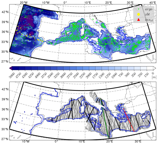
Figure 1 Top panel: Model domain and bathymetry. Green and yellow dots indicate the position of the assimilated ARGO floats and XBT respectively. Red triangles indicate the subset of in-situ data assimilated during the single daily cycle of 11 August 2021. Bottom panel: an example of 21 d altimetry data. Satellite tracks in red and green are used in Figs. 2 and 6 respectively. The solid, bold black tracks highlight the satellite altimetry data available during the single daily assimilation cycle of 11 August 2021. Three isobaths are drawn in both panels: 150, 350 and 1000 m.

Starting from an operational analysis, we performed a 1-year simulation followed by one year of daily assimilation cycles of in-situ (XBT and ARGO floats) and satellite SLA data for the whole year of 2021. Figure 1 shows the positions of the assimilated in-situ and SLA data. The SLA data coverage in the bottom panel refers to the full 21 d repeat cycle of the satellite orbits. In our experimental setup we perform daily assimilation cycles starting at midnight every day and we assimilate all observations available in the 24 h before the analysis time. The figure also highlights the data used during a single daily cycle (11 August 2021), specifically showing the in-situ and SLA track subset daily coverage.

4.1 Correcting the misfits for tides

A fundamental aspect to consider when assimilating SLA is the possible presence of tides in the modelled solution and in the observed data. Discrepancies between modelled and observed tides can, as a first approximation, be attributed to inaccuracies in the bathymetry of the model, the bottom and/or the coastal frictional dynamics. If the difference between observed and modelled estimates is due to tides, then this part of the misfit is primarily composed of external gravity waves. In the present OceanVar2 formulation, this high-frequency signal would be incorrectly projected into baroclinic increments by the covariance matrix of the background error (Eq. 3). Since tidal errors are not dynamically linked to the slow baroclinic ocean state, using the standard B matrix leads to spurious analysis increments. It is therefore essential to filter out the tidal signal from both the observed and modelled SLA. This work offers a solution to the assimilation of satellite altimetry in a model with tides, showing that a filtering procedure can be accurate enough and that no additional adjustment is required in the analysis.

The Copernicus along-track sea level anomalies are provided together with an estimate of the tidal signal along the tracks so tides can be filtered easily from the observations. To remove the tidal signal from the model background field, the tidal amplitude and phase for the eight components included in the Mediterranean Sea model (M2, S2, K1, O1, N2, P1, Q1 and K2) have been derived from a simulation output by harmonic analysis of the hourly sea level field. Following Cao et al. (2015), six months of hourly data were used for the harmonic analysis. The harmonic analysis was performed using the Pawlowicz et al. (2002) algorithm, based on the Foreman method (Foreman, 1977, 1978) at each model grid point. Knowing the tidal constants, it is possible to estimate the model tidal sea level at the exact time and location of the altimetry data and remove this component from the model outputs.

During the model simulation, misfits between model estimates and observations are computed and before entering OceanVar2, the misfits are updated, removing the tidal signal from both observations and model results. In Fig. 2 an example of an SLA satellite track is provided with model estimates and the satellite observations, the position of the track is shown in Fig. 1. In the upper panel of Fig. 2, the full signal from the model simulation and the observations is drawn as a function of latitude along the track. The middle panel of Fig. 2 shows the signals without tides, in addition to a debiasing procedure described by Dobricic et al. (2012). Dobricic et al. (2012) show that this method is the best for considering differences between the large-scale steric signal and the mean dynamic topography between observations and model. The average difference along the track is removed if the track is continuous, or for individual segments if the track is discontinuous due to the presence of land. Finally, in the bottom panel of Fig. 2 the two tidal components for the observational and modelled SLA are shown indicating the large-scale signal of tides in the open ocean.

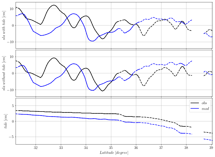
Figure 2 An example of Sea Level Anomaly data along the red track of Fig. 1. Blue lines indicate model free-run results, while black lines indicate observational data. In the upper panel the full signals are plotted. The dashed line indicates where SLA are in regions shallower than 1000 m. The middle panel shows the SLA after the removal of the tidal signals, separately in the model and observations, and the along-track averaged difference. The bottom panel shows the along-track observational and model tidal signals.

4.2 Sensitivity experiments

In addition to a free-run (non-assimilative model simulation), we present results from two sets of six 1-year assimilative experiments each, comparing them against each other and against observations. All the experiments assimilate ARGO floats and XBT temperature and salinity data in the whole domain including the Atlantic part, while SLA data are assimilated only within the Mediterranean Basin (see Fig. 1). In every experiment the vertical component of the background error covariance matrix is modelled using 25 tri-variate EOFs (temperature, salinity and SLA) computed following Dobricic et al. (2006) for every model grid point. The EOFs are computed from a 30-year timeseries of the Mediterranean Sea reanalysis (Escudier et al., 2021). The horizontal correlation radius was set to a constant value of 27 km, determined through sensitivity experiments. The diffusive filter was iterated five times to model the horizontal covariance. To account for coastal effects, the correlation radius was linearly decreased starting from about 30 km offshore to the minimum grid resolution near the coast. Additionally, a Neumann boundary condition was applied at the coast, setting the normal derivative of the field to zero. Observations are rejected if they are less than 15 km from the coast and if the misfits are larger than fixed thresholds: 5 °C for temperature, 2 psu for salinity; and 30 cm for SLA. The observational error covariance matrix is assumed diagonal. The results presented in Fig. 2 demonstrate that our model accurately reproduces along-track SLA tidal gradients, with the difference between the modelled and observed tidal signal being nearly constant. We effectively remove this along-track bias by subtracting the mean residual along each satellite track. This critical step ensures that the resulting misfit is very similar to the one computed without tides. Based on these considerations, we decided not to modify the SLA observational error, maintaining consistency with previous work (Escudier et al., 2021). Consequently, all the SLA data have an associated error of 3 cm regardless of the satellite and the geographic distribution. The observational errors for in-situ observations were tuned via the Desroziers' method (Desroziers et al., 2005) and vary monthly. We first prescribed the observation errors used in the previous system. The assimilation system was then run repeatedly, using the innovations and residuals to apply the Desroziers' formula to obtain an estimate for the observation error R. This process was iterated until the errors converged (e.g., Escudier et al., 2021). The resulting vertical error profiles are as follows: temperature and salinity observational errors peak at the surface with values of 0.45 °C and 0.14 psu, from 75 to 325 m depth they decrease linearly to values of 0.2 °C and 0.05 psu, starting from 750 m they have constant values of 0.1 °C and 0.02 psu respectively.

In addition to these sensitivity experiments, we also performed a set of idealized tests with synthetic observations to verify the internal consistency of the assimilation system and assess the behaviour of misfits and residuals under controlled conditions. A detailed description of these verification experiments is provided in the Supplement.

In all the experiments, the state vector contains the following model state variables:

$$\mathit{x}={\left[T,S,u,v,\mathit{\eta }\right]}^{\mathrm{T}}$$

where T is the three-dimensional temperature field, S the three-dimensional salinity field, u and v are the total horizontal velocity components and η the two-dimensional sea surface height.

Two sets of experiments are performed to compare the operational stability of mass-field-only $\left(T,S,\mathit{\eta }\right)$ correction against the maximal impact of full-state variable $\left(T,S,u,v,\mathit{\eta }\right)$ correction. Each of the two sets consists of six individual experiments (Exp-1 through Exp-6) with different OceanVar2 sea level operators and choices of free parameters. In Exp-1, which is used as a reference experiment, the barotropic model is used as the sea level operator with constant (in space and time) α and β in Eq. (7) and SLA data are rejected when falling in areas shallower than 100 m. In the second experiment (Exp-2), consistently with Adani et al. (2011), we rejected SLA data falling in areas shallower than 150 m. Experiment 3 is similar to Exp-2, but we test the sensitivity to variable expansion and contraction coefficients in Eq. (7). The coefficients are computed by linearizing the equation of state around a monthly mean climatology. In all these three experiments we integrated the barotropic model for 3 d with a time-step of 3600 s and then used the average of the last day as an approximation of the steady state solution. The integration of the barotropic model is fully implicit and the turbulent viscosity is equal to 650 m² s⁻¹.

Experiments 4, 5 and 6 use the dynamic height as the sea level operator. The difference between them is the choice of the level-of-no-motion. In Exp-4 we used a level-of-no-motion equal to 150 m, thus Exp-2 and Exp-4 differ only for the sea level operator. This shallow depth was specifically chosen to test the upper limit of observation inclusion, ensuring that the assimilation scheme uses the maximum possible Sea Level Anomaly (SLA) data coverage, even in areas shallower than the generally accepted level-of-no-motion. In Exp-5 the level-of-no-motion is 350 m in agreement with the Mean Dynamic Topography (Rio et al., 2014) used. Finally, in Exp-6 the level-of-no-motion is set at 1000 m which is the traditional choice for the operational setting of the Mediterranean Sea forecasting system (Coppini et al. 2023). In all these experiments, the depth of the level-of-no-motion naturally coincides with the minimum depth of SLA observations inclusion in the data assimilation scheme.

The configuration of the six individual experiments (Exp-1 to Exp-6) is identical across both sets. The two sets of experiments are designed to test the critical operational trade-off between numerical stability and maximal observational impact. In the first set of experiments, we prioritize stability by applying the analysis increments only to the assimilated variables (T, S and η), even though the state vector contains the velocity field. This forces the model dynamics to adjust the velocities indirectly. In the second set of experiments, which tests the maximal assimilation scope, also velocity corrections are applied directly in the analysis step. Throughout the remainder of the manuscript, experiments marked with an asterisk refer to those with velocity corrections. The first sets of experiments are summarized in Table 1. The second set of experiments has the same naming convention as the first set, with the sole difference being the application of the velocity correction in the analysis definition.

Table 1 Sensitivity experiments configurations. First row indicates the sea level operator used: BM = Barotropic Model; DH = Dynamic height. Second row indicates the choice for expansion and contraction coefficients: constant in space and time (Const) and spatially and temporarily variable as computed from monthly climatology (MC). Third row indicates the reference level for the lower integral limit of the dynamic height operator and thus the level-of-no-motion for the V_u,v part of the model background error covariance matrix. Fourth row indicates the minimum depth used as criterion to reject SLA data.

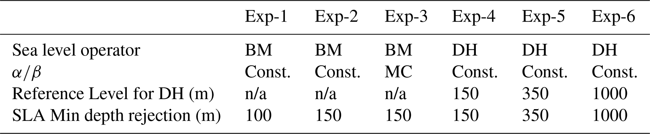
n/a – not applicable.

4.3 Performance Metrics

To fully assess the performances of the experiments listed in Table 1, the mean squared error (e.g., Murphy, 1988) is decomposed and the single components are analysed:

$$\begin{array}{}\text{(10)}& {\displaystyle }\mathrm{MB}=\stackrel{\mathrm{‾}}{m}-\stackrel{\mathrm{‾}}{o},\text{(11)}& {\displaystyle }\mathrm{SDE}={\mathit{\sigma }}_m-{\mathit{\sigma }}_o,\text{(12)}& {\displaystyle }\mathrm{CC}={\displaystyle \frac{\mathrm{1}}{{\mathit{\sigma }}_o}}{\displaystyle \frac{\mathrm{1}}{{\mathit{\sigma }}_m}}{\displaystyle \frac{\mathrm{1}}{N}}\sum _{i=\mathrm{1}}^N\left(m_i-\stackrel{\mathrm{‾}}{m}\right)\left(o_i-\stackrel{\mathrm{‾}}{o}\right),\end{array}$$

where MB is the mean bias error, SDE is the standard deviation error and CC is the cross correlation between the modelled and observed fields. The ith modelled and observed variable is denoted by m_i and o_i, respectively; $\stackrel{\mathrm{‾}}{m}$ and $\stackrel{\mathrm{‾}}{o}$ are the respective averages (horizontal and temporal); while σ_m and σ_o are the respective standard deviations. In addition, the unbiased root mean squared error (uRMSE) is computed:

$$\begin{array}{}\text{(13)}& \mathrm{uRMSE}=\sqrt{{\displaystyle \frac{\mathrm{1}}{N}}\sum _{i=\mathrm{1}}^N{\left[\left(m_i-\stackrel{\mathrm{‾}}{m}\right)-\left(o_i-\stackrel{\mathrm{‾}}{o}\right)\right]}^{\mathrm{2}}}.\end{array}$$

It is important to note that the model results and observations used here are the same as those used to calculate misfits within the assimilation cycle. However, while not all misfits are utilized in the assimilation process, all available observations are included in the error statistics. This ensures that all experiments are evaluated based on the same reference dataset of observations. Furthermore, to evaluate model performance even in very shallow regions, the observational dataset used in the misfits, and thus in the calculation of the error statistics, includes sea level anomaly (SLA) data covering regions up to 10 m depth. This allows for the assessment of model skill in very shallow regions where data are not assimilated in any of the presented experiments.

Given that the CC is always positive for all the experiments, the misfit statistics for the experiments listed in Table 1 are also analysed in terms of relative improvement with respect to the free-run or Exp-1 according to the following metrics definition:

$$\begin{array}{}\text{(14)}& {\displaystyle }{S}_{{\mathrm{uRMSE}}_{\mathrm{Exp}\mathrm{\#}}}=\left({\displaystyle \frac{{\mathrm{uRMSE}}_{\mathrm{Ref}}-{\mathrm{uRMSE}}_{\mathrm{Exp}\mathrm{\#}}}{{\mathrm{uRMSE}}_{\mathrm{Ref}}}}\right)\times \mathrm{100},\text{(15)}& {\displaystyle }{S}_{{\mathrm{CC}}_{\mathrm{Exp}\mathrm{\#}}}=\left({\displaystyle \frac{{\mathrm{CC}}_{\mathrm{Exp}\mathrm{\#}}-{\mathrm{CC}}_{\mathrm{Ref}}}{{\mathrm{CC}}_{\mathrm{Ref}}}}\right)\times \mathrm{100},\end{array}$$

where # indicates the different experiments listed in Table 1 and “Ref” denotes the free-run or Exp-1. S_CC is only calculated using Exp-1 as the reference. The exclusion of the free-run as a reference is necessary because the very small CC values would lead to excessively large percentage values that hinder meaningful comparison between the different experiments. In the manuscript the relative performance statistics are presented only for the SLA data given that a similar comparison for the temperature and salinity did not provide additional insights.

5 Results

Figure 3 shows the temperature and salinity increments resulting from different assimilation scheme setups (Table 1), all starting with the same set of SLA misfits. These increments are presented before analysing the skills of the various experiments. The differences between the experiments are generally small, and of the order of 10 %. The largest differences are due to the different number of SLA data assimilated, a result of the constraint imposed by the level-of-no-motion used or the different minimum depth rejection criterion adopted. We note that when the same data are assimilated, thus in areas deeper than 1000 m, very similar increments in SLA are generated by the OceanVar2 regardless of the schemes adopted. However, the schemes differ on how these increments are projected into temperature and salinity increments. Note that the ordinate axes are strongly stretched in the figure to highlight the first 150 m depth where most of the corrections are confined. Comparing Exp-2 and 3, which differ only in the use of spatially and temporally variable expansion and contraction coefficients, we observed small but noticeable differences in the temperature and salinity increments, particularly in the amplitude of near-surface maxima. The choice of sea level operator substantially influenced the results. When using Dynamic Height with a level-of-no-motion set at 1000 m (Exp-6), temperature and salinity increments were comparable to those obtained with the barotropic model. The primary cause of the observed differences appears to be the constraint imposed on assimilated data by the level-of-no-motion. Reducing the level-of-no-motion (Exp-4 and 5) allowed for the assimilation of more sea level anomaly data but resulted in considerably different temperature and salinity increments within the first 100 m compared to the barotropic model.

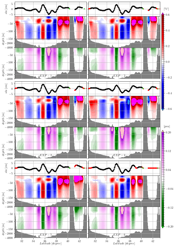
Figure 3 SLA, Temperature (red/blue) and Salinity (magenta/green) increments obtained from the different OceanVar2 configurations listed in Table1, starting from the same misfits. The SLA track used is drawn in green in Fig. 1. For each experiment in the top panel there are the SLA increments where black dots indicate assimilated data, green dots indicate data rejected based on the coastal distance criteria, red dots indicate data rejected due to the level-of-no-motion or minimum depth (in case of the barotropic model).

5.1 Barotropic sea level operator and free-run comparison

The performance of Exp-1 is compared with free-run. In Fig. 4 the statistics for the SLA are shown. Every point in the time-series represents 5 d window statistics. That is, the overbars and the standard deviations in Eqs. (10), (11), (12) and (13) are computed over a 5 d time window.

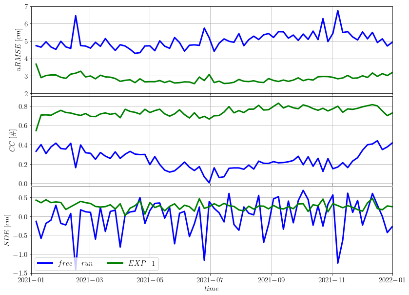
Figure 4 Time series of SLA error statistics for the entire year 2021. Blue (“free-run”) and green (“EXP-1”) lines indicate the statistics for the free-run results and the misfit of Exp-1 respectively. Top panel: unbiased root-mean-square error. Middle panel: correlation coefficient, in the bottom panel the standard deviation error is plotted.

The free-run has an error of about 5 cm, slightly growing during the second half of the year. The model with assimilation underwent a 10–20 d adaptation period, after which the uRMSE of the misfit stabilizes around 3 cm. A consistent improvement is noted in the CC. No seasonal cycle is observed in the CC of Exp-1, whereas the free-run exhibits a distinct summer minimum in the correlations. The SDE in the free-run is on average negative and it is characterized by 5 d oscillations. In Exp-1, the SDE stabilized around values of 0.25 cm, indicating an overestimation of the observed variability.

The SLA yearly averaged statistics were clustered according to ocean bathymetry and are plotted in Fig. 5. In areas with bathymetry between 150 and 2500 m, the free-run exhibited an almost constant uRMSE. However, the error increases in shallower and deeper regions, reaching the maximum in areas deeper than 3500 m. The uRMSE of the Exp-1 was more stable and approximately half of the corresponding free-run statistics. Regardless of the region considered, Exp-1 has better statistics than the free-run, indicating the effectiveness of the assimilation procedure. For the CC differences between free-run and Exp-1 results are also evident. In the free-run CC decreases with depth, while for the Exp-1 we observe an opposite tendency. In terms of SDE, the largest improvements with respect to the free-run are in shallow areas. The free-run underestimates the variance in areas with bathymetry shallower than 1000 m, this is particularly evident in areas shallower than 150 m. The model with data assimilation tends to overestimate the observed variability particularly in shallow areas.

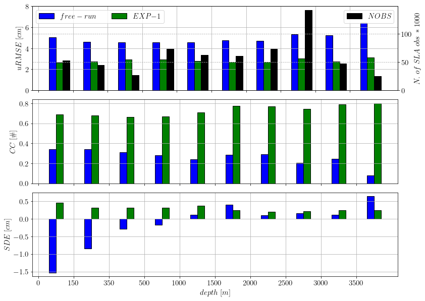
Figure 5 SLA statistics as a function of the ocean depth. Blue and green bars indicate the free-run and Exp-1 results respectively. In the top panel the number of observations used is also provided with dark bars.

In Fig. 6 the vertical profiles of uRMSE, MB, CC and SDE for salinity (upper panels) and temperature (bottom panels) for the free-run and the Exp-1 are shown. Statistics are computed against all available ARGO and XBT profiles. The vertical structure of the salinity uRMSE is similar between the free-run and the Exp-1. The salinity errors are characterized by a near surface maximum which is reduced in the assimilative run. The MB in the free-run has a subsurface minimum at 100 m depth, while Exp-1 misfits have almost homogenous values through all the water column. The CC resembles the vertical distribution of the uRMSE, with values approaching the unity in both the experiments below 500 m depth. Finally the salinity SDE confirms the large improvement arising from the assimilation procedure. In the near surface layer, the free and the assimilative run have opposite behaviours, with the free-run overestimating the observed variability while the assimilative run underestimating it. Below 100 m depth the SDE salinity values of Exp-1 are noticeably reduced with respect to the free-run.

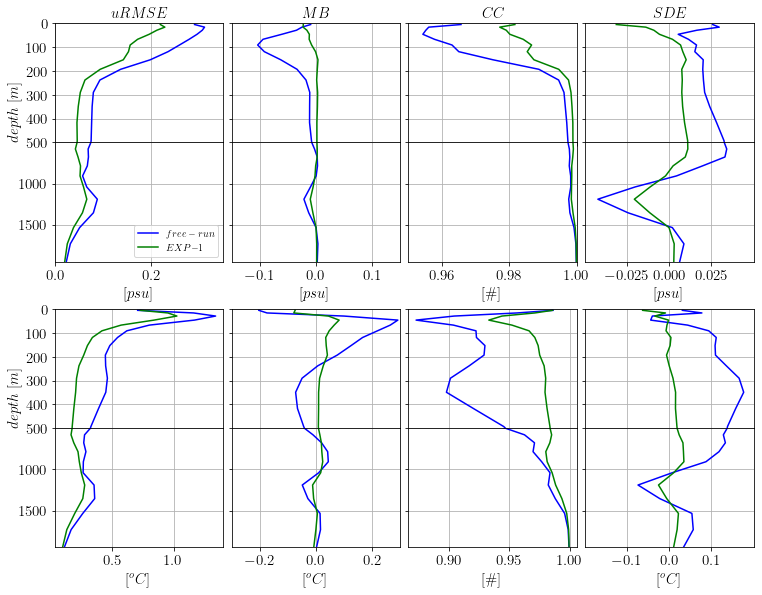
Figure 6 Vertical profiles of yearly averaged misfit statistics for salinity (top panels) and temperature (bottom panels). From left to right: uRMSE, ME, CC and SDE. Blue and green lines indicate free-run and Exp-1 results respectively.

The temperature uRMSE and CC are characterized by a strong, summer intensified (not shown), subsurface maximum/minimum due to the model difficulties in reproducing the correct stratification. A second uRMSE local maximum (CC minimum) is present around 300 m probably related to the misrepresentation of the Levantine Intermediate Water (LIW) advection in the different Mediterranean regions. A third temperature error relative maximum is present between 1000 and 1500 m depth. The assimilation corrects all the errors by approximately 30 %–50 % down to 500 m, less below this depth.

Temperature MB is largely improved by assimilation. The free-run tends to overestimate the observed temperature variability, and the SDE has a marked vertical structure. In general, the assimilation seems capable of correcting most of the model errors except in the upper thermocline/mixed layer depth. Analysis of the corresponding time-series (not shown) indicates a clear summer maximum in all the error statistics in proximity of the mixed layer depth. This behaviour is shared between all the different experiments, but it is clearly reduced in the assimilative runs. However, the persistence of this error maximum suggests a limitation in the current formulation of the Background Error Covariance. Specifically, the static, climatological nature of the EOFs used to model the vertical error component struggles to fully capture the rapidly evolving stratification and strong vertical gradients characteristic of the summer mixed layer. Future development will prioritize replacing these EOFs with more dynamic and stratification-aware operators to address this deficiency.

5.2 Sensitivity experiments to the sea level operator

Figure 7 illustrates the performance of the six different data assimilation experiments (without velocity corrections) in terms of correlation coefficient (CC) and improvements in root-mean-square error (S_uRMSE) relative to the model free-run. The top panels display the time evolution of these improvements, highlighting both short-term fluctuations and overall trends. The bottom panels present the time-averaged S_uRMSE and CC clustered by bathymetric depth ranges, revealing how the effectiveness of each experiment varies with depth. All assimilative experiments outperformed the model free-run. Experiments using the dynamic height as the sea level operator, with levels of no motion set at 150 m (Exp-4) or 1000 m (Exp-6), generally performed worse than the other experiments. For Exp-6, the differences in both uRMSE and CC were particularly noticeable in regions shallower than 1000 m, where SLA data were not assimilated. However, even in these regions, Exp-6 substantially outperformed the model free-run, suggesting that corrections applied in deeper areas effectively propagated into shallower regions. In Exp-4, the deterioration in results compared to other experiments was primarily confined to deeper regions. In areas shallower than 150 m Exp-1 outperforms the other experiments, however the performances of the experiments are similar indicating that the coastal areas are strongly constrained by the open ocean dynamics. A clear dependence of the CC on model bathymetry was evident in all experiments with the most significant improvements (with respect to the free-run) observed in areas deeper than 3500 m, where the model free-run exhibited the smallest CC. In shallow regions, Exp-6 generally provided the smallest improvement in CC compared to the other experiments. The results demonstrate that certain experiments achieve substantial improvements in deep-ocean regions, while others show more consistent performance across all depths. These results highlight the challenges associated with choosing an appropriate level-of-no-motion in data assimilation of SLA. The requirement to define a spatially constant level-of-no-motion, which is inherent to the dynamic height operator, demonstrates the critical limitations imposed by its theoretical assumptions, and our experimental results explicitly highlight these deficiencies. This constraint imposes a critical methodological compromise. For instance, maintaining a conservative, deep level-of-no-motion (e.g., 1000 m in Exp-6) ensures physical consistency but mandates the exclusion of a large fraction of the available SLA observations. Conversely, adopting a shallower level-of-no-motion (e.g., 150 m in Exp-4) maximizes observation coverage, yet the resulting analysis is compromised due to the violation of the theoretical assumptions in deeper water, ultimately leading to degraded accuracy. The choice of the level-of-no-motion can significantly impact the accuracy of model analysis, especially in complex regions with varying bathymetry and ocean dynamics, thereby confirming the methodological advantage of the barotropic model operator which successfully assimilates all available SLA data without imposing a constant level-of-no-motion constraint.

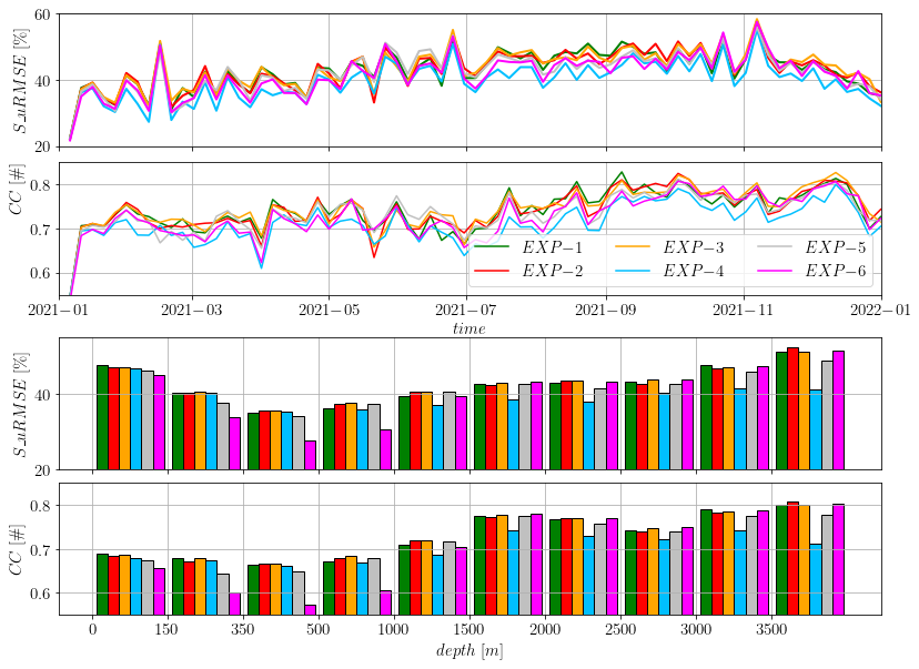
Figure 7 S_uRMSE and CC indices for the SLA misfit errors for the different experiments. S_uRMSE is computed w.r.t the free-run. Top two panels: time-series. Bottom panels: average indices for bathymetry classes.

Figure 8 presents the relative performance of five data assimilation experiments (Exp-2 through Exp-6) compared to a baseline assimilative experiment (Exp-1), now used as the reference. The top panels illustrate the time series of the relative change in root-mean-square error (S_uRMSE) and correlation coefficient (S_CC). The bottom panels depict the time-averaged S_uRMSE and S_CC changes, categorized by bathymetric depth ranges. In contrast to the previous figure, where improvements were relative to a model free-run, this figure demonstrates the relative performance of each experiment against the initial data assimilation run. Negative values indicate a decrease in performance (higher uRMSE or lower CC) compared to Exp-1, while positive values indicate improvement. This comparison highlights the incremental benefits or drawbacks of different experimental configurations in relation to a specific data assimilation configuration.

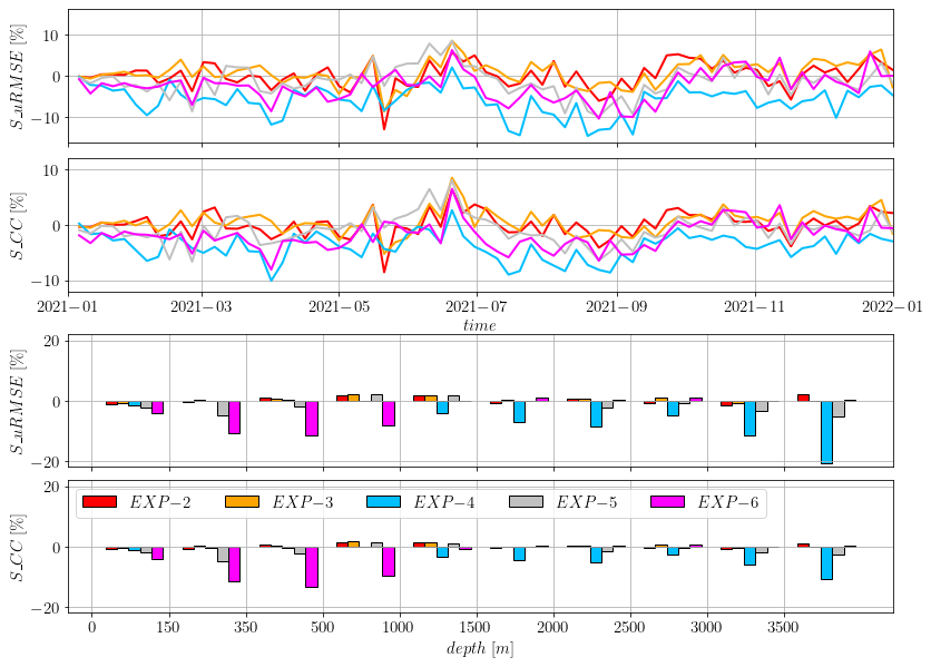
Figure 8 S_uRMSE and S_CC indices for % of improvement of the SLA errors for the different experiments w.r.t Exp-1. Top two panels: time-series. Bottom panels: average indices for bathymetry classes.

All the experimental configurations employing the barotropic model perform similarly to each other. In terms of time-series comparison, Exp-4 (with dynamic height as sea level operator and level-of-no-motion equal to 150 m) has performance worse than all the other experiments. Among the experiments using the dynamic height operator, Exp-5 generally has better results both in terms of uRMSE and CC. The analysis per bathymetric class highlights the differences among the experiments. None of the experiments outperform Exp-1 in regions shallower than 150 m both in terms of uRMSE and CC. In deeper areas we see that Exp-4 and Exp-5 produce, in general, worse results, and the worsening is amplified as the depth increases and the level-of-no-motion decreases; 1000 m depth is a clear boundary for the effectiveness of Exp-6. Employing the barotropic model as a sea level operator yields consistent results, with small sensitivity to the minimum depth used in the rejection criterion or to the choice of constant or variable expansion/contraction coefficients. This confirms the difficulty of establishing a constant level-of-no-motion and highlights the benefit of using the barotropic model as a balancing mechanism.

5.3 Sensitivity experiments to velocity corrections

The second set of experiments (Exp-1^* to Exp-6^*) was carried out including velocity corrections in the analysis estimates. This second set represents the maximal scope of multivariate assimilation, providing a benchmark against the mass-field-only correction of the first set. The OceanVar2 configuration used in Exp-4^* generated velocity increments that led to numerical instabilities in the ocean model, preventing this simulation from completing. This critical instability confirms the operational risk associated with introducing direct momentum corrections and highlights the sensitivity of Exp-4. In contrast, the other experiments in this set ran without such issues, underscoring the challenges associated with dynamic height methods. Consequently, our focus is on the stable experiments. Across all the stable configurations, the successful experiments in the second set, which included velocity corrections, demonstrated improved performance compared to their counterparts in the first set, without velocity corrections. The extent of improvement varies depending on the specific experiment and the region analysed.

Figure 9 shows the time series and Fig. 10 presents temporally averaged statistics by bathymetric class for the second set of experiments. In terms of time series (Fig. 9), the error components exhibit the same characteristics as those discussed for Exp-1 (Figs. 4 and 5). The uRMSE exhibits a summer minimum in all experiments. Exp-6^∗ performs significantly worse than the others throughout the year. All experiments using the barotropic model have similar uRMSE values, with Exp-1^∗ generally appearing slightly better than the others. The correlation coefficient (CC) increases throughout the experiment's length. For this statistic as well, Exp-6^∗ is the worst, showing consistently lower values than the other experiments. Even for the SDE, which is generally reduced compared to the previously studied experiments without velocity corrections, the relative performance of the different experiments is confirmed.

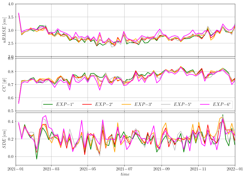
Figure 9 Second set of experiments SLA time series error statistics. Top panel: unbiased root-mean-square error. Middle panel: correlation coefficient. Bottom panel: standard deviation error. Colour code is provided in the middle panel legend.

Figure 10 presents the temporally averaged statistics clustered according to the bathymetry. All the stable experiments benefited greatly from the inclusion of the velocity corrections. The overall reduction in error confirms the importance of the velocity increments when the system remains stable. Exp-6^∗ confirms its poor performance in areas shallower than 1500 m. However, by also correcting the velocities, its statistics in deep areas are now similar or slightly better than those obtained from experiments using the barotropic model as operator in the background error covariance matrix. Exp-1^∗ is now the best among those analysed for all the bathymetric classes shallower than 500 m.

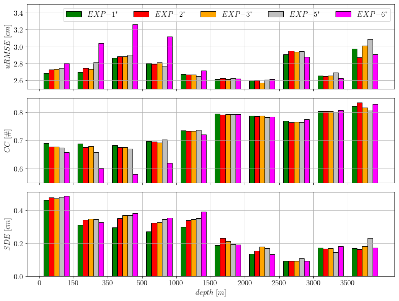
Figure 10 SLA statistics as a function of the ocean depth. Top panel: unbiased root-mean-square error. Middle panel: correlation coefficient. Bottom panel: standard deviation error. Colour code is provided in the top panel legend.

In terms of correlation coefficient, the results previously obtained by analysing uRMSE seem to be confirmed. For shallow areas (<1000 m), Exp-6^∗ is significantly worse than the others. In all other bathymetric classes, while confirming the previous findings, the differences between the experiments are less pronounced. A different behaviour is observed when analysing the standard deviation of the error. Exp-1^∗ remains the configuration that shows significantly lower error values than the others in almost all bathymetric classes. Notably, Exp-6^* is the one that benefits the most from velocity corrections, demonstrating that for this specific configuration, the direct momentum increments overcome other methodological weaknesses.

6 Computational performance and parallelization

To improve computational performance, OceanVar2 adopts a domain-decomposition scheme. This scheme leverages the computing power of a parallel computer by partitioning the computational domain into subdomains. Each process executes the necessary operations to update its portion of the global domain, sharing communications with neighbouring processes for lateral boundary treatments using Message Passing Interface (MPI) calls (The MPI Forum, 1993).

Rigorous testing has been conducted to guarantee bit-for-bit (BFB) reproducibility for the entire data assimilation system, excluding the cost function minimizer, across runs with different MPI processes as well as runs with the same amount of MPI processes but different partitioning of the structured geographic grid. The quasi-Newton L-BFGS minimizer (Byrd et al., 1995), employed for numerical minimization of the cost function, necessitates global matrix-vector multiplication, which precludes BFB reproducibility when domain decomposition is utilized. Divergences between executions stem from the non-associativity of floating-point operations, particularly floating-point summation within the minimizer. To specifically test and ensure that the parallelization of the rest of the assimilation system is fully reproducible, OceanVar2 offers the flexibility to execute the minimizer serially (by aggregating variables from all domains and forcing a fixed order of operations) while the remaining code is parallelized using MPI domain decomposition. Extensive testing has demonstrated that using this specific serial option for the minimizer ensures BFB reproducibility. Moreover, even when the minimizer is executed in parallel, differences arising from various domain decompositions are statistically insignificant. Possible future work includes the introduction of a different minimizer suited for MPI parallelization.

Neglecting the differences arising from the parallel execution of the minimizer, the computational performance of the different experiments was evaluated in terms of minimizer iterations and code scalability. Figure 11 compares the number of iterations required for the minimizer to converge in the various OceanVar2 experiments. The results are presented as a probability distribution, with statistics calculated based on the year of assimilation testing. Consistently, all experiments using the dynamic height operator converged with fewer iterations than those employing the barotropic model. The choice of the level-of-no-motion had a small effect, where the median increased from 24 to 25 iterations when using 350 or 150 m instead of 1000 m. However, the primary insight is that the choice of the free surface operator formulation and the level-of-no-motion have negligible impact on the overall convergence speed. The median number of required iterations remains stable across all the experiments, varying only from 24 to 26 iterations. These differences between the median values appear insignificant when considered in the context of the wide day-to-day variability in the required convergence steps observed across the assimilation year, which spans approximately 12 to 45 iterations due to fluctuation in data availability and associated misfit values. The observed increase in the median number of iterations for the barotropic model schemes is likely due to the barotropic model's inherent physical complexity, which results in a more intricate optimization landscape for the minimizer to navigate.

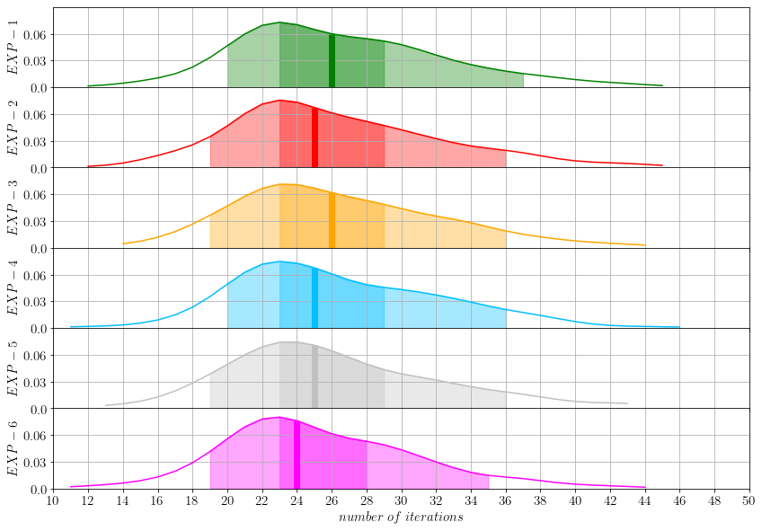
Figure 11 Probability density function (y axis) of the number of iteration (x axis) needed for the OceanVar2 minimization algorithm to converge. For each experiment, the lighter and darker shaded areas correspond to the 90 % and 50 % of the events respectively. The vertical lines are the medians of each distribution. Exp-1 to Exp-6 from top to bottom.

To assess scalability, we limited the comparison to Exp-2 and Exp-4, as they had the same number of assimilated observations. We tested OceanVar2's performance with increasing numbers of cores. For a fixed number of cores, we performed experiments using eight different sets of observations and various decomposition strategies. (e.g., with 16 cores, we tested 4×4 and 8×2). The results are shown in Fig. 12. The model grid consisted of $\mathrm{1307}\times \mathrm{380}\times \mathrm{141}$ points along the x, y, and z directions, respectively. Analysis not shown here confirms that, in these experiments, the computational load across subdomains does not show significant differences based on geometric peculiarities, such as coastal proximity. Instead, the computational load of a subdomain, and thus the total execution time, was primarily determined by the overall number of assimilated observations. This finding is consistent with the global nature of the variational solver and the number of iterations required for convergence. Notably, subdomains completely covered by land still required execution time comparable to the other domains. This occurred as a direct result of the land-sea mask not being used to optimize the domain decomposition, since the decomposition was based solely on the model grid geometry. The top panel of Fig. 12 shows the CPU time per core as a function of the number of cores for Exp-2 and Exp-4. Consistently with Fig. 11, the solid lines, representing the average CPU time, indicate that the difference between the dynamic height scheme (Exp-4) and the barotropic model (Exp-2) operators is minimal across all core counts, especially considering the large variability in run times, evidenced by the shaded areas indicating the maximum and minimum CPU time. More importantly, the speedup achieved is limited; increasing the cores from 1 to 36 yields a speedup of approximately 8, corresponding to a parallel efficiency of about 22 %. Furthermore, both experiments reach a performance plateau around 36 cores, with run time generally deteriorating at higher core counts due to increased communication overhead.

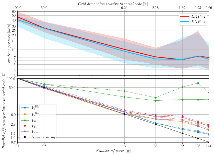
Figure 12 Parallel performance and routine-level scalability. Top panel: CPU time per core (minutes) as a function of the number of cores for Exp-2 and Exp-4. Solid lines represent the average CPU time, while shaded areas indicate the maximum and minimum CPU time observed for each core count. Bottom panel: Scalability analysis of individual Background Error Covariance matrix components. The y-axis is the percentage of reduction time with respect to the serial (single core) execution. Solid lines indicate the minimum execution time and dashed lines indicate the maximum execution time observed across different days and domain decompositions for both the tangent linear and adjoint routines. The solid black line indicates the linear reduction with the number of cores, and coloured lines show the performance of individual routines (component colours are defined in the figure legend).

To understand this limited parallel efficiency, the bottom panel of Fig. 12 presents the scalability (expressed as a percentage of efficiency relative to the serial code) for the different B matrix operators. The diffusive filter operator acts as the main bottleneck. Its efficiency decreases rapidly at higher core counts and then exhibits a negligible further performances gain, stabilizing beyond 36 cores. This filter, which utilizes an implicit scheme, was implemented using a dimensional splitting approach. It is solved by means of LU decomposition of a tridiagonal matrix. We acknowledge that the implementation and parallelization strategy employed is suboptimal. This design choice simultaneously precludes optimal parallelization and results in the diffusive filter's extreme sensitivity to the geometry of the domain decomposition, which is the primary cause of the wide run-time variability shown in the top panel. This sequential process requires all processors associated with subsequent columns of subdomains to wait and then repeats along the second dimension (rows of subdomains). Although this crude, initial implementation constrains the overall parallel efficiency, the resulting total execution time remains within acceptable limits, rendering the software suitable for our current purposes. Future development will prioritize a more scalable parallelization strategy for this critical routine. Examining the remaining key operators reveals a strong general trend: while efficiency is high up to 36 cores, all remaining components experience a reduction in scaling performance thereafter. The barotropic model operator is the least affected by this change in scaling efficiency observed past 36 cores, maintaining the highest efficiency among the B operators.

7 Conclusions

This study describes recent developments of the OceanVar software which implements an incremental variational ocean data assimilation scheme. Key innovations compared to the previous schemes (DP08, Storto et al., 2011, 2016) include the implementation and evaluation of two alternative solutions for the sea level operator, encompassing both barotropic model and dynamic height operator. Furthermore, a diffusive operator has been adopted to model Gaussian horizontal covariances, replacing the recursive filter used in previous code versions. Finally, the geostrophic velocity operator is utilized for total velocity corrections, deviating from the DP08 approach and applied to both dynamic height and barotropic sea level operators.

Furthermore, a method for filtering the tidal components of the background model fields is applied and tested allowing the assimilation of SLA without tides, together with in-situ temperature and salinity data to produce analyses. These new and old features in OceanVar2 have been tested and compared for a regional implementation of the assimilation scheme in the Mediterranean Sea.

It has emerged that the barotropic operator is the only operator capable of consistently assimilating sea level anomaly data in shallow and deep ocean regions. Variable α and β parameters in the linear equation of state (7) yielded minor differences in our experiments, however this assumption is likely not to be valid in global models.

The dynamic height operator, though easy to implement, has clear limitations. Requiring the definition of a spatially independent level-of-no-motion, it does not provide an optimal solution in domains with highly variable bottom topography and dynamics. For the Mediterranean Sea, a level-of-no-motion equal to 1000 m is appropriate, as demonstrated by the quality of the corrections obtained with OceanVar2. However, this represents a significant limitation, as it excludes the assimilation of SLA observations in shallower areas. Decreasing the level-of-no-motion depth reveals the limitations of this approach. For shallower levels, the benefits of assimilating more data are offset by the loss of the quality of the corrections in deeper areas. The results are corroborated by the numerical instabilities arising when velocity corrections are applied in experiments with a level-of-no-motion shallower than 350 m. The emergence of this critical instability provides a clear empirical demonstration that violating the inherent physical consistency assumptions used to construct the B matrix can lead to unstable solutions. Consequently, the optimal choice of operator depends on balancing the need for maximal observational impact with the requirement for numerical stability within the specific operational framework.

Although the barotropic model is inherently more complex and thus computationally more expensive than the dynamic height operator, its impact on the total run time is minor. This is because the semi-implicit scheme used to discretize the barotropic equations allows for large time-steps, significantly limiting the computational demand. This small computational overhead ensures that the barotropic model operator does not become the dominant factor in execution time.

The adopted solutions simplify the application of OceanVar2 in complex areas of the world's oceans. To our knowledge OceanVar2 is the only data assimilation software employing a barotropic model in its model background error covariance matrix. It is important to note that the current implementation of the barotropic model uses closed lateral boundary conditions. Its applicability is therefore limited to basins with a geometry that allows this approximation. In the future the barotropic model will be implemented also with open boundary conditions.

Regarding parallel performance, the diffusive filter overhead is currently the dominant computing factor, constraining the overall scalability. We acknowledge that the first implementation of the diffusive filter used in OceanVar2 limits the system's parallel efficiency. However, we chose this direction, replacing the previously used recursive filter, due to the superior flexibility and adaptability the diffusive filter offers for modeling horizontal error correlations.

The mathematical and algorithmic core of the system, first presented in DP08 and subsequently used in various operational forecasting frameworks, has been largely documented in several scientific works. Based on extensive testing, the revised code is stable and robust, with its performance results presented throughout this work. The present version, OceanVar2, is also open to the community.