Scenario set-up and the new CMIP6-based climate-related forcings provided within the third round of the Inter-Sectoral Model Intercomparison Project (ISIMIP3b, group I and II)

This paper describes the climate-related forcings (CRFs), i.e. change in climate comprising the atmosphere and the ocean, coastal water levels, and atmospheric composition (CO₂ and methane concentrations), provided as input data within the “b” part of the third simulation round of the Inter-Sectoral Impact Model Intercomparison Project (ISIMIP3b). While ISIMIP3a comprises historical impact models simulations forced by observational Direct Human Forcings (DHF), such as changes in population and asset distributions, land use, fishing efforts, agricultural and water management driven by socio-economic development or climate protection strategies, and observational CRF, the ISIMIP3b CRFs are based on climate model simulations generated within the sixth phase of the Coupled Model Intercomparison Project (CMIP6). In a first set of experiments covering the pre-industrial (1601–1849) and historical period (1850–2014) (ISIMIP3b, group I) the CMIP6-based CRFs for the historical period are combined with historical observation-based DHF also considered in ISIMIP3a. These group I simulations allow for the quantification of impacts of historical climate change by comparison to simulations where the observational DHF are combined with simulated pre-industrial CRFs. In addition, the impacts of observed changes in CRFs can be compared to the impacts of simulated changes in CRFs by comparing the ISIMIP3a simulations to the ISIMIP3b, group I simulations. The second group of experiments (ISIMIP3b, group II) comprises future projections assuming constant observational direct human forcings at 2015 levels to estimate the impact of climate change given today's DHF for the low emission scenario SSP1-2.6, the high and the very high emission scenarios SSP3-7.0, SSP5-8.5, and reference simulations based on pre-industrial CRF, respectively. The very high emissions scenarios and the assumption of fixed present day DHF particularly allow for testing the scalability of impacts in terms of global temperature change. The provided CRFs comprise atmospheric CO₂ and CH₄ concentrations, atmospheric and oceanic climate data, coastal water levels, tropical cyclone (TC) tracks and their associated wind speed and precipitation fields. In addition to the CRFs data, this paper describes the experiments belonging to group I and II and the rationale behind them. Another set of future projections accounting for changing DHFs (ISIMIP3b, group III) is in preparation and will be described in another paper.

1 Introduction

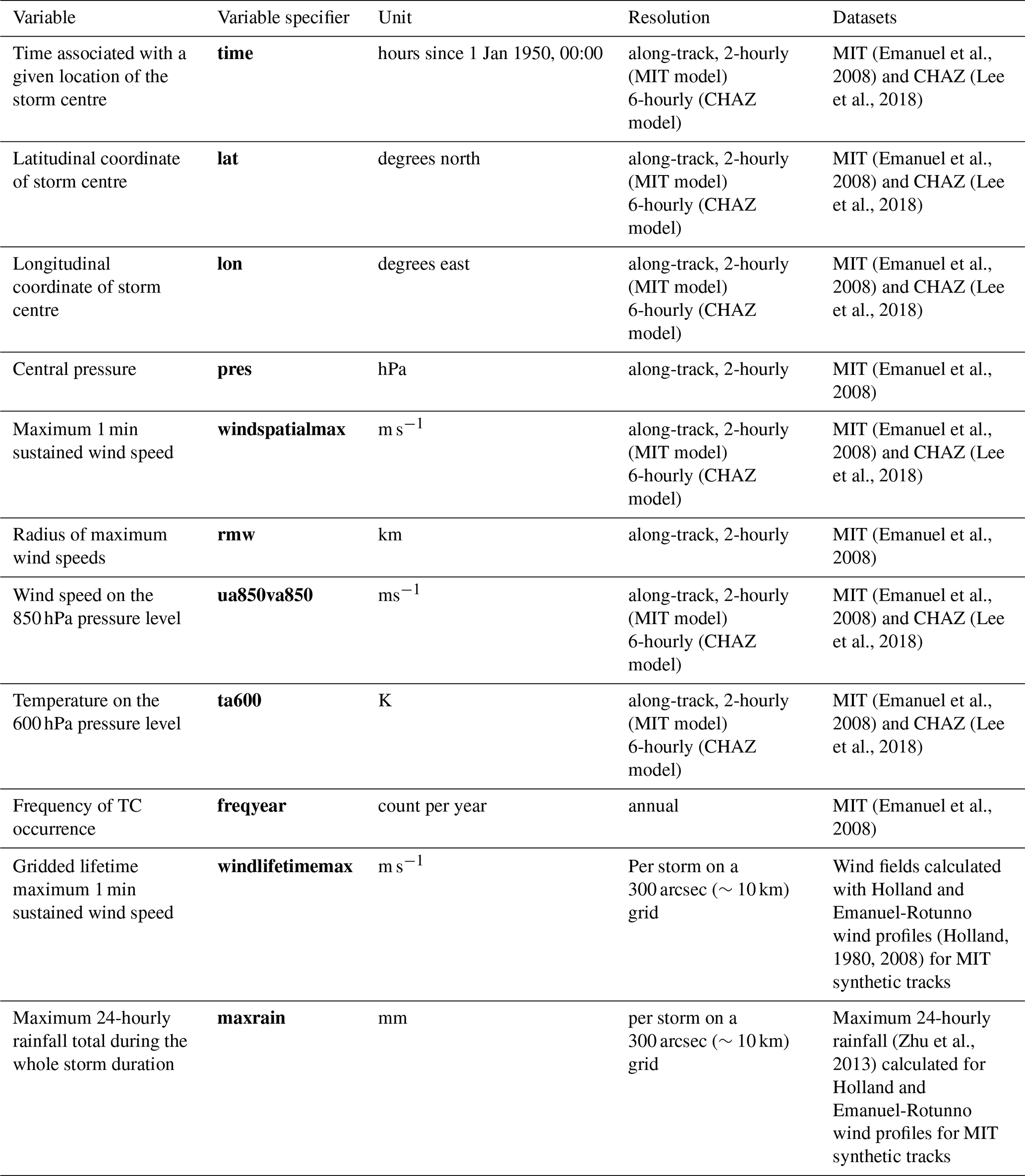
This is the second paper of a series of three papers describing the experiments of the third simulation round of the Inter-Sectoral Impact Model Intercomparison Project ISIMIP (isimip.org). The project provides a common scenario framework for cross-sectorally consistent climate impact simulations. Here, the term “experiment” is used as synonym for “scenario-setup”, i.e. the specification of the impact model simulations in terms of the applied input data or additional assumptions determining the simulations. This is following the use of the term within other model intercomparison projects such as the Coupled Model Intercomparison project CMIP (CMIP Model and Experiment Documentation, 2026) and a longer tradition within ISIMIP. Within ISIMIP the experiments are determined by the underlying set of CRFs and DHF. The CRF is different from the “climate forcing” considered within climate models. For the impact models the associated climate change represents the forcing. In addition, some of the impacts (e.g. changes in natural vegetation and crop yields) also directly depend on CO₂ concentrations (CO₂ fertilization effect, increased water use efficiency). Others (coastal infrastructure models) need information about sea level rise as input. Following the terminology of the IPCC AR6, where climate-related systems are defined as the “climate system including the ocean and the cryosphere as physical or chemical systems” (O'Neill et al., 2022), we label this group of forcings as Climate-Related Forcings (CRF) that cover all the inputs listed in Table 1. This group is distinguished from the Direct Human Forcing induced by socio-economic development, mitigation strategies or human adaptation measures such as land use changes, changes in agricultural and water management, population and assets distributions. While this paper only introduced the CRF for the ISIMIP3b, group I + II experiments a list of inputs belonging to this second group of forcings can be found in Frieler et al. (2024).

Currently, operational simulation protocols exist for the following sectors: Agriculture, Biomes, Energy, Fire, Food security and nutrition, Groundwater, Labour, Lakes global, Lakes regional, Fisheries and marine ecosystems global, Fisheries and marine ecosystems local, Peatland, Permafrost, Water global, Water regional. Additional protocols for Coastal systems, Regional forests, Temperature-related mortality, health indicators, Terrestrial biodiversity, and Water quality sectors are under development.

In its third round it covers (i) model evaluation and climate impact attribution experiments based on observation-based CRF and DHF (ISIMIP3a, Table 1 of the associated protocol paper (Frieler et al., 2024), (ii) climate impact simulations driven by simulated CRF based on climate model simulations generated within the sixth phase of the Coupled Climate Model Intercomparison Project (CMIP6) (see Table 1, this paper) assuming ISIMIP3a observational DHF in the historical period and fixed 2015 DHF for the future simulations (ISIMIP3b, group I + II, this paper), and (iii) an upcoming set of CMIP6-based future projections where DHF vary according to given Shared Socioeconomic Pathways (SSPs) (no adaptation scenarios) and in response to climate change impacts (adaptation scenarios) (ISIMIP3b, group III). So while this paper only describes the ISIMIP3b CRF, the first paper described the historical DHF used within ISIMIP3b, and the third paper will only address the future DHFs for group III that are still under development while the CRF of the group III simulations will be identical to the future CRF described here.

Similar to the Coupled Model Intercomparison Project (CMIP) (Eyring et al., 2016) all simulations will be freely available (ISIMIP Repository, 2026) to allow for follow-up analysis. The consistent design of the simulations does not only allow for the comparison of climate impact simulations within each sector, but also enables the bottom-up integration of impacts across sectors. Thus, it provides a unique basis for the estimation of the effects of climate change on, e.g., the economy, displacement and migration, health, or water quality resolving the mechanisms along different impact channels and fully exploiting the process-understanding represented in the biophysical impact models.

Compared to the CMIP5-based ISIMIP2b, the ISIMIP3b CRF represent the following updates: (i) climate forcing data based on phase 6 of the Coupled Model Intercomparison Project (CMIP6) (Eyring et al., 2016) and post-processed by an improved bias adjustment and statistical downscaling method (see Sect. 3.2), and (ii) provision of large ensembles of potential realisations of tropical cyclone tracks, wind and precipitation fields derived from two different modelling approaches assuming CMIP6 boundary conditions, while in ISIMIP2b only one approach was used and precipitation fields were not included. In addition, we plan to provide coastal water levels at high temporal resolution (upcoming). The approach to generate the data is also described here.

The development of the ISIMIP3b protocol was coordinated by the ISIMIP-Cross-Sectoral Science Team (CSST) at the Potsdam Institute for Climate Impact Research (PIK) along the same decision process as for ISIMIP3a (Frieler et al., 2024).

This paper is accompanied by a simulation protocol (ISIMIP3b simulation protocol, 2026) providing all technical details such as file and variable naming conventions, as well as sector-specific output variables to be reported by the participating modelling teams. As the protocol may still be updated due to addition of new variables, correction of errors, or the inclusion of new sectors, contributors to ISIMIP should always refer to https://protocol.isimip.org (last access: 20 December 2025) for the most up to date reference for planned impact model simulations.

The ISMIP3a and ISIMIP3b protocols have been jointly developed and participation in ISIMIP3 requires contribution to both ISIMIP3a and ISIMIP3b, using the same impact model versions in order to allow for the evaluation of the impact models future projections in ISIMIP3b.

The paper provides a catalogue where interested modellers can find the data to run their models according to the ISIMIP3b protocol.

In Sect. 2, we describe selected scenarios and the rationale behind the individual set-ups chosen within the community-driven decision process (Sect. 2). In Sect. 3, we then introduce the individual climate-related forcing data sets collected as input for the different modelling experiments covering atmospheric climate data including lightning and tropical cyclones tracks, wind and precipitation fields; ocean data; coastal water levels; and atmospheric CO₂ as well as CH₄ concentrations. We provide a brief documentation of the approaches, variable names, formats, references, sources, covered time period, etc., as a service to the community, without analysing and discussing these datasets, except for the effects of an adjustment of the bias-adjustment method used to generate the ISIMIP3b atmospheric forcing data (see Sect. 3.1).

2 Experiments and underlying rationale

The selection of the scenarios is a community-driven process constrained by the availability of climate model simulations (ensemble of simulations by multiple General Circulation Models (GCMs) per scenario) and socio-economic background information (such as land use patterns, populations and GDP data etc. additionally required as “Direct Human Forcing” for the ISIMIP3b, group III impact model simulations that will be introduced in an upcoming paper). These criteria have made CMIP6-ScenarioMIP the reference point for the selection (O'Neill et al., 2016). The selection of ISIMIP3b scenarios (see Fig. 1) from the four ScenarioMIP Tier 1 scenarios was additionally driven by the aim to capture a wide range of possible futures from low to high emission scenarios and to provide a long baseline simulation assuming pre-industrial climate conditions that allows for a robust estimation of reference return levels of extreme events. This is why the original selection comprised the pre-industrial baseline (“picontrol”), the historical simulations (“historical”), SSP1-2.6 representing the “low end of the range of future forcing pathways in the IAM literature”, and SSP5-8.5 representing the “high end of the range of future pathways in the IAM literature” (O'Neill et al., 2016). Given recent mitigation efforts, some estimates of recoverable coal reserves, and decreasing prices for renewable energies the emissions underlying SSP5-8.5 have been criticised for being unplausibly high (Emissions – the “business as usual” story is misleading, 2023). Based on these discussions, the “medium to high end of the range of future forcing pathway” SSP3-7.0 (O'Neill et al., 2016) has been added to the ISIMIP3b scenario set-up. While this scenario is described as “average no policy” by Hausfather and Peters (2020) (Emissions – the “business as usual” story is misleading), we highlight that we explicitly do not describe it as a “business as usual scenario” and that this was not the framing within ScenarioMIP either. Instead SSP3-7.0 differs from the other scenarios with regard to particularly high aerosol emissions and high decreases in forest areas going beyond the assumptions in the other scenarios. So it has been shown that the increase of global mean precipitation with global warming is much weaker in SSP3-7.0 than in the other scenarios (Shiogama et al., 2023). In addition, SSP5-8.5 is explicitly kept in the ISIMIP3b ensemble as its particularly strong warming signal allows testing to what degree the simulated impacts of climate may scale with global mean temperature, which could allow for a translation of impacts to other emission scenarios. In addition, even under lower emission scenarios, global warming levels as the ones reached under SSP5-8.5 in 2100 will eventually be reached later in time as long as emissions are not reduced to zero. These impacts of high warming levels would not be captured when only considering lower emission scenarios ending in 2100.

However, in such a setting it has to be taken into account that ssp370 is different from the other scenarios with regard to particularly high aerosol emissions and high decreases in forest areas going beyond the assumptions in the other models. So it has been shown that the increase of global mean precipitation with global warming is much weaker in SSP3-7.0 than in the other scenarios (Shiogama et al., 2023).

All ISIMIP experiments are determined by the underlying set of CRFs and DHF, where each package of CRF and DHF has a specific label that will then be included in the output file names to allow for an identification of the experiments they belong to. The individual experiments are defined by the combination of both types of forcing data sets, where the associated specifiers are indicated in brackets in the subheadings naming the experiments (CRF specifier + DHF specifier). The different combinations of the default sets of ISIMIP3b CRFs (“picontrol”, “historical”, “ssp126”, “ssp370”, and “ssp585”) and DHF (“histsoc”, “2015soc”, “1901soc”, “1850soc”, “nat”, and “2015soc-from-histsoc”) are sketched in Fig. 1 and described in more detail below.

The CRF data described in this paper are mandatory; i.e. if impact models consider this forcing, the specified dataset must be used; if an alternative input data set is used instead, the run cannot be considered an ISIMIP3b, group I + II simulation. The DHF for the historical period is identical to the ISIMIP3a DHF listed in Table 1 of Frieler et al. (2024) where we also indicate whether the data set is mandatory or optional. Optional forcing data could be used but is not mandatory. In addition, the protocol includes a set of sensitivity experiments that are described as deviations from the default runs and labelled by the baseline CRF and DHF settings and a third specifier indicating the deviation from this default setting. The ISIMIP3b group I + II sensitivity scenario set-ups include experiments with fixed levels of atmospheric CO₂ concentrations (“2015co2”), high levels in CO₂ concentrations in combination with low levels of climate change (“ssp585co2”), and lightning data that vary in response to climate change (“varlightning”), while lightning is fixed at present day levels in the default runs. These sensitivity experiment runs are not depicted in Fig. 1 but listed in Table 2.

Figure 1 Illustration of the default ISIMIP3b forcing data sets. Each ISIMIP3b experiment is defined by a combination of a CRF data set with a DHF data set. The considered combinations are listed in Table 2 and the underlying rationale is described in Sect. 2.1 and 2.2. Table 1 lists all data sets defining the considered CRFs while the DHFs are based on the same datasets as in ISIMIP3a. Potentially required spin-up procedures are not included in the figure, but described in Sect. 2.1.

The ISMIP3b simulations are divided into two groups. Group I comprises the simulations from 1601–1849 (pre-industrial) and 1850–2014 (historical) assuming simulated pre-industrial and historical CRFs and different constant (“nat”, “1850soc”, and “2015soc”) or varying (“histsoc”) levels of DHF based on the same observational data used in ISIMIP3a (see Fig. 1). Group II comprises the future projections assuming constant 2015 levels of DHF (see Fig. 1) including a baseline with pre-industrial CRF (grey line in the future projections part of Fig. 1). All experiments are introduced in more detail below (Sect. 2.1 for group I and 2.2 for group II).

In contrast to ISIMIP3a, the CRFs provided for ISIMIP3b currently only comprise atmospheric (see Sect. 3.1) and oceanic climate data (see Sect. 3.4), tropical cyclone tracks with associated wind and precipitation fields (see Sect. 3.2), and CO₂ and methane concentration (see Sect. 3.5). We do not yet provide associated coastal water levels (see Sect. 3.2.3 for planned work). Impact simulations that rely on the missing forcings cannot be generated within ISIMIP3b yet, but we are currently developing their setup and will provide the forcings as soon as possible. The ISIMIP3b atmospheric and oceanic climate data are derived from five different GCMs generated within the Coupled Model Intercomparison project, phase 6 (CMIP6).

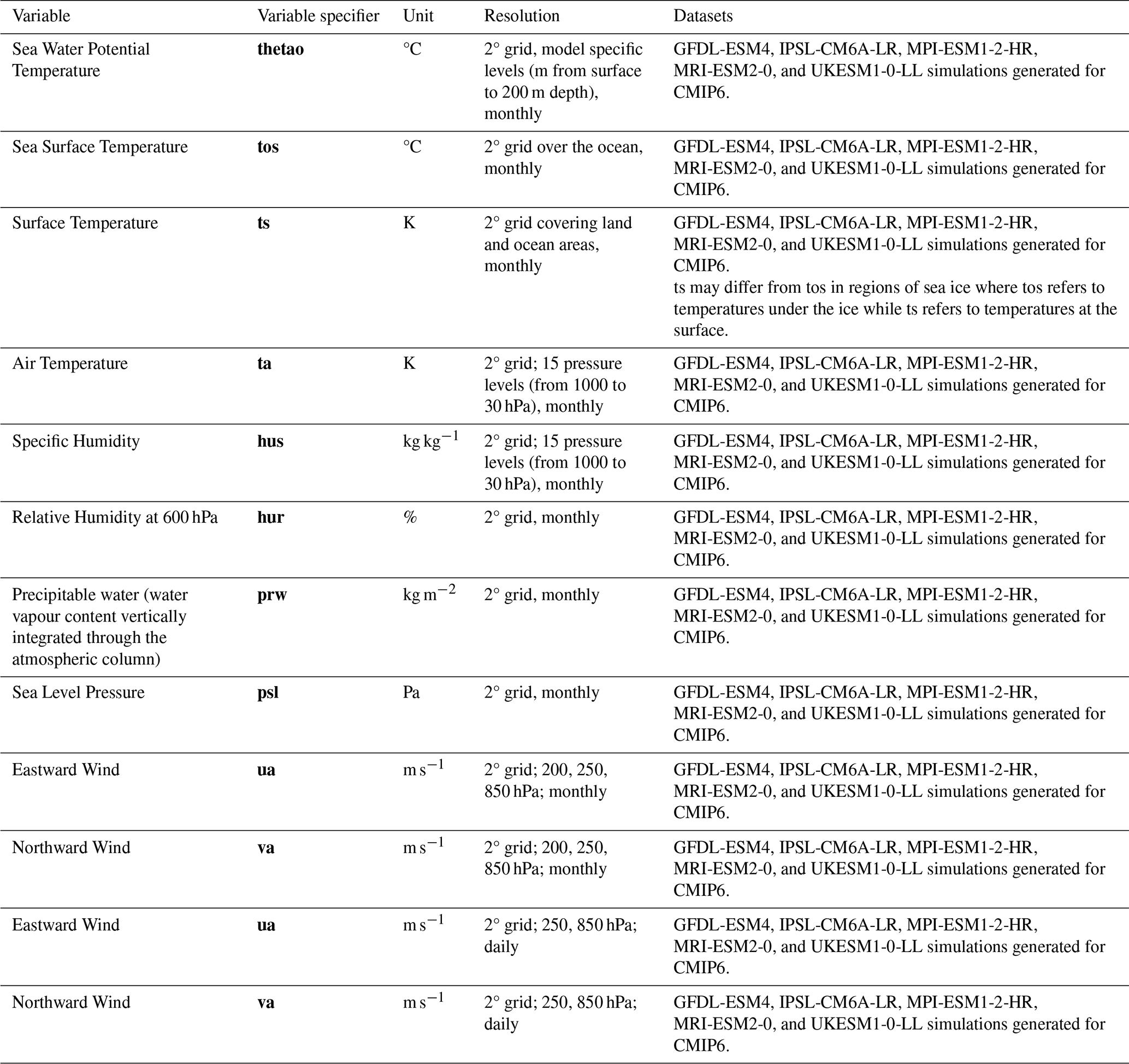
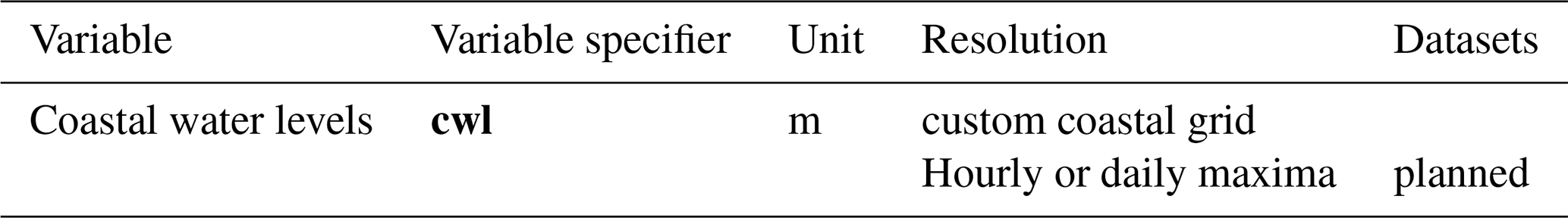
Table 1 Climate-Related Forcing datasets for ISIMIP3b. Climate-Related Forcing datasets for ISIMIP3b; forcing groups are set in bold, forcings in italic, and the single data sets in regular font.

2.1 ISIMIP3b, group I: Climate-model based impact model simulations for the period from 1601 to 2015

The group I experiments cover the years 1601–1849 with pre-industrial CRFs (“picontrol”) and fixed 1850 direct human forcings (“1850soc”) described in the grey column 3 of the ISIMIP3b scenario Table 2 as well as the subsequent years 1850–2014 considering pre-industrial and historical CRF (“picontrol” or “historical”) and different assumptions about DHF (“histsoc”, “2015soc”, “1850soc”, and “nat”) as described in the grey column 4 of Table 2. The reasoning behind the individual experiments are introduced below.

Pre-industrial reference simulations (picontrol + histsoc, picontrol + 2015soc, picontrol + 2015soc-from-histsoc, picontrol + 1850soc, picontrol + nat; default)

To estimate the impacts of historical and future changes in the CRFs, the protocol includes reference simulations based on pre-industrial CRFs and DHF identical to those considered in the climate change scenario runs. These reference simulations represent large samples (at least 250 years) of impact distributions based on stable pre-industrial CRFs (picontrol) and constant DHFs (see “picontrol + 1850soc”, “picontrol + 2015soc”, and “picontrol + nat” experiments in Table 2). Compared to the often used much shorter historical reference periods, this allows for a more robust fitting of extreme value distributions such as Gumbel distributions to simulation of e.g. annual maximum discharge to estimate reference 100 year return levels.

In addition, the protocol includes a reference experiment for the historical period (1850–2014) with DHF changing over time (histsoc) and 1850–2014 pre-industrial CRF (picontrol), while fixed 2015 DHF is considered afterwards (2015–2100) (“picontrol + 2015soc-from-histsoc”). This run may be different from the “picontrol + 2015soc” simulation for this time window because of the lagged effects of increasing DHF from 1850 to 2014. The “histsoc” DHF is identical to ISIMIP3a (Frieler et al., 2024).

The complete pre-industrial reference runs are divided in two parts. Only the first parts from the start until 2014 belong to group I (grey fields in Table 2), while the second parts covering the period 2015–2100 belong to group II (red parts of Table 2).

Comparing these reference simulations to the scenario experiments using historical CRFs (historical + histsoc, historical + 2015soc, historical + 1850soc, historical + nat; default (see below)) allows for the estimation of the effects of simulated historical climate change conditional on the assumed DHF. The historical CRF (“historical”) starts from the pre-industrial climate simulation in 1850, i.e. the “picontrol” and “historical” versions of the experiments have a common starting point. As some impact indicators may have “internal” trends not necessarily forced by external drivers (e.g. re-growth of forests), the comparison of the 1850–2014 impact simulations forced by the “historical” CRF to parallel simulations using the “picontrol” CRF is more appropriate to estimate the effects of historical climate change than comparing an early period of the historical impact simulation to the end of the historical period. The comparison of the simulations assuming “historical” CRF with the reference simulations based on “picontrol” CRF does not allow for a separation of the impacts of the natural and anthropogenic historical climate forcing. To allow for a quantification of the effects of the anthropogenic CRFs, we also support historical reference simulation accounting for the natural CRF only (“hist-nat” simulations generated within the Detection and Attribution Model Intercomparison Project (DAMIP) as sub-MIP of CMIP6, (Gillett et al., 2016) While this set-up is not an official part of the ISIMIP3b protocol, we provide the associated bias-adjusted CRF as secondary climate input data (Lange et al., 2023).

For models requiring a spin-up, the “picontrol” CRFs should be used in combinations with DHF (i) at 1850 levels to spin-up for the “1850soc” and “histsoc” experiments, (ii) at 2015 levels to initialise the “2015soc” experiment, and (iii) set to zero to start the “nat” experiments. For the spin-up all years of the “picontrol” CRF should be copied as often as needed. The “picontrol + 1850soc” run from 1601–1849 is part of the regular experiments that should be reported and hence the spin-up has to be finished before this pre-industrial period.

Standard historical simulations based on historical climate-related forcing and observed changes in direct human forcing (historical + histsoc; default)

This experiment covering the historical period (1850–2014) is determined by historical (“historical”) CRFs and DHFs evolving according to observations (ISIMIP3a “histsoc” DHF). The ISIMIP3b “historical + histsoc” experiment is comparable to the default “obsclim + histsoc” experiment considered within ISIMIP3a but based on simulated CRFs. The simulated climate is different from the observed realisation due to differences in the internal variability of the observed and simulated historical climate and potential deficits in the climate model simulations or the observational data. A comparison between the default ISIMIP3b “historical + histsoc” impact model simulations to the associated ISIMIP3a results allows for a quantification of the effects of the discrepancies between the observed and simulated CRFs on the considered impact indicators. These simulations can be initialised from the spin-up of the associated pre-industrial reference simulations in case a spin-up is needed.

Simulations with historical climate-related forcing and fixed 2015 direct human forcing (historical + 2015soc; default)

This historical experiment is similar to the standard historical experiment except that it is forced by fixed 2015 DHF. It is introduced into the “first priority” scenario-set-up to generate an ensemble of historical cross-sectorally consistent impact simulations that is as large as possible by not excluding impact models that are not able to handle varying DHF. If a spin-up is needed the associated simulations can be initialised from the spin-up of the associated pre-industrial reference simulation (picontrol + 2015soc, default) described at the beginning of this section.

Simulations with historical climate-related forcing and fixed 1850 direct human forcing (historical + 1850soc; default)

This historical experiment is also similar to the standard historical experiment but it is forced by the fixed 1850 DHFs. It corresponds to the “obsclim + 1901soc” experiment of ISIMIP3a. Here in ISIMIP3b we consider the year 1850 instead of 1901 used in ISIMIP3a as this is the year where the “historical” climate simulations with observed natural and human forcings start, i.e. a branch from the pre-industrial climate simulations assuming constant pre-industrial forcings (“picontrol”). The “historical + 1850soc, default” impact model simulations allow for the quantification of the “pure effect of climate change” over the historical period. In contrast, the comparison of the “historical + 1850soc, default” impacts simulations to the “historical + histsoc” simulations allows for the quantification of the “pure effect of historical changes in DHF”. If a spin-up is required it does not have to be newly generated as it is identical to the spin-up for the default “picontrol + 1850soc”, “picontrol + histsoc”, and “historical + histsoc” simulations and described in the beginning of this section.

Simulations with historical climate-related forcing and no direct human forcings (historical + nat; default)

Considering no DHF (nature run) allows quantifying the effect of the simulated historical climate change conditional on otherwise natural conditions, i.e. no direct human influences on land use, water management etc.. This experiment is introduced as a companion experiment to the “obsclim + nat” experiment of ISIMIP3a. The comparison with the three historical simulations with constant DHF allows for testing to what degree the impact of climate change on the simulated natural or human systems is conditional on the underlying DHF. This experiment is only included for the biomes and fisheries and marine ecosystems fisheries sectors as models from other sectors usually need some basic information such as vegetation patterns that are not available for natural-only conditions. The biomes models generate their own natural-only vegetation patterns based on their dynamic representation of vegetation. A spin-up does not have to be newly generated but is identical to the spin-up for the “picontrol + nat” experiment described above.

“De-biased” sensitivity simulations within the marine ecosystems and fisheries sector (FishMIP) with de-biased historical oceanic forcings and no or histsoc direct human forcings (historical + nat, historical + histsoc; de-biased)

So far, the default oceanic forcing is not bias-adjusted as globally the observational data are too sparse to be used in a similar empirical way as for the bias-adjustment of the atmospheric forcing. However, the biases in the forcing are expected to also induce biases in the historical and future impact simulations. To quantify these effects and to test a suggested bias-adjustment method based on comprehensive ocean-biogeochemistry model simulations forced by bias-adjusted atmospheric forcings we include a sensitivity experiment where the default CRF is replaced by input data generated by a dynamical de-biasing approach (Lengaigne et al., 2025) using the NEMO-PISCES physical-biogeochemical ocean model (Madec, 2015), which is the oceanic component of the IPSL-CM6A-LR climate model. Thus, the forcing data will first be generated for IPSL-CM6A-LR, but later extended to other ISIMIP-GCMs as described in Sect. 3.4.2.

In contrast, the oceanic forcing for the regional component of the marine ecosystems and fisheries sector have been bias-adjusted by regional observational oceanic data as described in Sect. 3.4.3. In this case most models only use the bias-adjusted inputs and not the raw ones. Nevertheless the experiments are labeled as “de-biased” sensitivity experiments to ensure a consistent naming across scales.

2.2 ISIMIP3b, group II: Climate-model based future impact model simulations with constant 2015 direct human forcings

The ISIMIP3b, group II simulations comprise a set of future impact projections (2015–2100) using fixed levels of DHF as considered in the historical simulations (“2015soc”, “1850soc”, and “nat”) or reached at the end (2014) of the historical period in the “historical + histsoc” runs (“2015soc-from-histsoc”). These runs are described in the red cells of Table 2.

Pre-industrial reference simulations (picontrol + 2015soc, picontrol + 2015soc-from-histsoc, picontrol + 1850soc, picontrol + nat; default)

These simulations are included into the ISIMIP3, group II part of the protocol to allow for the estimation of the effect of climate change by comparing the future impact projections to simulations assuming the same background DHF but pre-industrial levels of CRF (see description of baseline simulations in Sect. 2.1).

Future impact projections assuming SSP-RCP-based climate-related forcings starting from “historical + histsoc” simulations (ssp126 + 2015soc-from-histsoc, ssp370 + 2015soc-from-histsoc, ssp585 + 2015soc-from-histsoc; default)

This experiment represents an expansion of the group I “historical + histsoc” experiment based on fixed 2015 DHF for the future. Note that this experiment is different from the experiment with fixed 2015 DHF for the future where the associated impact simulations start from the “historical + 2015soc” group I simulations (see description below).

These experiments have been introduced to describe the impacts of different scenarios of changes in the climate-related systems on today's natural systems and societies, i.e. assuming present day population levels and distributions, land use patterns, water, and agricultural management measures etc. In many cases, the projected changes in natural and human systems can be interpreted as the pure effect of the prescribed changes in the climate-related systems. However, they could also partly result from lagged effects of the historical changes in DHFs (“histsoc”), CRF (“historical”), or natural temporal trends induced e.g. by re-growth of forests. To be able to separate natural trends from the effects of changing CRFs, the associated simulations can be compared to reference impact simulations with pre-industrial CRF forced with the same DHF (“picontrol + 2015soc-from-histsoc”, see description in group I section).

Future impact projections assuming SSP-RCP-based climate-related forcings starting from historical simulations with constant 2015 direct human forcings (ssp126 + 2015soc, ssp370 + 2015soc, ssp585 + 2015soc; default)

These experiments expand the “historical + 2015soc” experiments from ISIMIP3b, group I using DHFs that are held constant at 2015 levels for the historical period into the future. Although the DHF in the future period is identical to the future simulations described above, the difference in historical forcing may affect the impact simulations in the future period. These simulations are also considered first priority as some of the impact models may not be able to handle varying DHF and therefore can only perform these experiments. Models participating in the “2015soc-from-histsoc” experiments described above are also asked to complete the “2015soc” runs to generate an ensemble of consistent impact model simulations with as many members as possible.

Future impact projections assuming SSP-RCP-based climate-related forcings starting from historical simulations assuming constant 1850 direct human forcings (ssp126 + 1850soc, ssp370 + 1850soc, ssp585 + 1850soc; default)

These experiments continue the default “historical + 1850soc” experiments considered in ISIMIP3b, group I. They are included to estimate the impact of changes in the climate-related systems conditional on 1850 levels of DHF that can be compared to the impact conditional on today's levels of DHF (“2015soc”).

Future impact projections assuming SSP-RCP-based climate-related forcings starting from historical simulations assuming no direct human forcings (ssp126 + nat, ssp370 + nat, ssp585 + nat; default)

These experiments continue the default “historical + nat” experiments in ISIMIP3b, group I. They are included to estimate the effect of changes in the climate-related systems (here climate change itself and increasing CO₂ concentrations) assuming no DHF.

CO₂ sensitivity simulations (ssp126 + 2015soc-from-histsoc, ssp370 + 2015soc-from-histsoc, ssp585 + 2015soc-from-histsoc, ssp585 + 2015soc, ssp585 + 1850soc, ssp585 + nat; 2015co2)

To separate the effects of increasing atmospheric CO₂ concentrations (in particular the CO₂ fertilisation or water use efficiency effects on vegetation) from the effects of other changes in the climate-related systems, the ISIMIP3b protocol includes sensitivity experiments where atmospheric CO₂ concentrations are held constant at 2015 levels. For SSP1-2.6 and SSP3-7.0, they are only introduced as deviations from the default “2015soc-from-histsoc” experiments while for SSP5-8.5 the effect can also be quantified conditional on all levels of direct human influences considered in the previous experiments.

Future lightning sensitivity simulations (ssp126 + 2015soc-from-histsoc, ssp370 + 2015soc-from-histsoc, ssp585 + 2015soc-from-histsoc; varlightning)

To study the effects of future changes in lightning flash rates as opposed to using a stationary lightning climatology, the ISIMIP3b protocol includes sensitivity experiments where future lightning flash rates change along the RCPs. The future lightning data sensitivity experiment is introduced as a deviation from the default “2015soc-from-histsoc” experiment and only for one climate model (UK-ESM). This sensitivity experiment has been introduced for the fire sector.

Climate sensitivity simulations under high levels of CO₂ (ssp126 + 2015soc-from-histsoc, ssp585co2)

To study the effects of high atmospheric CO₂ concentration without accompanying changes in climate, the ISIMIP3b protocol includes a sensitivity experiment where the atmospheric CO₂ concentration are prescribed according to RCP8.5, while the other CRF, in particular the atmospheric forcings are from SSP1-2.6. The future climate sensitivity experiment is introduced as a deviation from the default “ssp126 + 2015soc-from-histsoc” experiment. This sensitivity experiment has been introduced for the peat sector.

“De-biased” sensitivity simulations within the marine ecosystems and fisheries sector (FishMIP) with de-biased oceanic forcings and no or 2015soc direct human forcings for reference simulations based on pre-industrial oceanic forcing (picontrol + nat, picontrol + 2015soc-from-histsoc; de-biased) and the associated simulations accounting for different levels of climate change (ssp126 + nat, ssp370 + nat, ssp858 + nat, ssp126 + 2015soc-from-histsoc, ssp370 + 2015soc-from-histsoc, ssp585 + 2015soc-from-histsoc)

These simulations represent the future extensions of the “de-biased” group I simulations described above. They are designed to test the dynamical bias-adjustment suggested for the global oceanic forcings under different levels of climate change (ssp126, ssp370, ssp585). The regional impact projections within the sector are also based on de-biased oceanic forcings and are therefore also labeled as “de-biased” sensitivity experiments to ensure a consistent labeling across scales.

Table 2 ISIMIP3b climate-model based experiments. The table provides a comprehensive list of all ISIMIP3b, group I (pre-industrial + historical period) and group II (future period) experiments defined by the assumed CRF and DHF. Here, the CRF are only described by the climate (oceanic and atmospheric) forcings and the assumed CO₂ and CH₄ concentrations that have a direct influence on the simulated impacts. Coastal water levels are not mentioned in the description as we do not provide the associated input data yet. Experiment specifiers are set in bold.

3 Climate-related forcing data

3.1 Bias-adjusted and statistically downscaled atmospheric climate forcing

For ISIMIP3b we provide the daily atmospheric forcings for the same variables as in ISIMIP3a on the default 0.5° grid (see Table 3). These variables are from the output of CMIP6 climate model simulations, selected and processed as described below. We use the climate simulations from the picontrol (for pre-industrial conditions), historical (for historical conditions), ssp126, ssp370, and ssp585 (for future conditions under the scenarios SSP1-2.6, SSP3-7.0, and SSP5-8.5, respectively) CMIP6 experiments.

Table 3 Climate-related atmospheric forcing data provided within ISIMIP3b. The upper limits of precipitation (pr) and snowfall (prsn) correspond to 600 and 300 mm d⁻¹, respectively, while the lower and upper limits of Near-Surface Air Temperature (tas), Daily Maximum Near-Surface Air Temperature (tasmax) and Daily Minimum Near-Surface Air Temperature (tasmin) correspond to −90 and +70 °C, respectively. Variable specifiers are set in bold.

For the pre-industrial conditions, 500 years of picontrol output data are used and harmonised across GCMs with respect to the time range they cover. This is possible because picontrol data only carry nominal year labels without historical reference points (see original nominal start and end years in Table 4). We changed the GCM-specific picontrol time ranges listed to 1601–2100.For the historical and future climate conditions, we provide input data for 1850–2014 and 2015–2100, respectively, in line with the time ranges covered by the corresponding CMIP6 experiments. The common time axis is important as the use of the input data should be harmonised across all sectors. In particular, the year-by-year combination of the pre-industrial CRF with the historical DHF should be done in the same way across all sectors and models.

Selection of climate models

To limit the number of mandatory impact simulations and hence lower the barrier to participation in ISIMIP3b, we provide climate input data for only five selected CMIP6 climate models. The basic characteristics of the five GCMs are listed in Table 4. The models were selected based on data availability at the selection time (late 2019 to early 2020), performance in the historical period, structural independence, process representation and equilibrium climate sensitivity (ECS).

To be included in ISIMIP3b, a GCM had to provide daily data for all variables listed in Table 3 except for near-surface specific humidity (huss) (which was derived from near-surface relative humidity (hurs), surface air pressure (ps) and near-surface air temperature (tas), see below), ps if sea level pressure (psl) was available, so a proxy for ps could be computed based on psl and tas, and near-surface wind speed (sfcwind) if zonal and meridional near-surface wind components (uas, vas) were available, so a proxy for sfcwind could be computed based on uas and vas. Those daily data had to cover 500 picontrol years and all years of the historical, SSP1-2.6, SSP3-7.0, and SSP5-8.5. In addition, we favoured GCMs that provided the additional input data needed for the tropical cyclone modelling (Table 5) and the fisheries and marine ecosystems sector (FishMIP; Table 10).

Table 4 Characteristics of CMIP6 climate models used in ISIMIP3b. Columns show (from left to right) the climate model acronym, the horizontal grid size (longitude × latitude) of the original atmospheric output data, the ensemble member used, the nominal time range covered by the picontrol data used, the equilibrium climate sensitivity (ECS) according to (Meehl et al., 2020), and the main model reference paper and the CMIP6 simulation data publications used. For definitions of climate model acronyms and modelling groups see (CMIP6 source_id values, 2023).

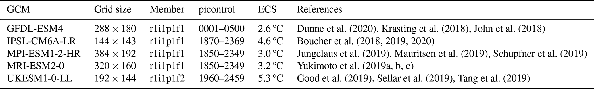
According to a skill analysis (see Fig. 2), the GCMs ACCESS-CM2, AWI-CM-1-1-MR, CESM2, CESM2-WACCM, CMCC-ESM2, EC-Earth3-AerChem, GFDL-CM4, GFDL-ESM4, HadGEM3-GC31-LL, HadGEM3-GC31-MM, MPI-ESM1-2-HR, MPI-ESM1-2-LR, MRI-ESM2-0, NorESM2-MM, SAM0-UNICON, TaiESM1, and UKESM1-0-LL perform relatively well in reproducing the main historically observed characteristics of the atmosphere. From that list, only GFDL-ESM4, MPI-ESM1-2-HR, MRI-ESM2-0, and UKESM1-0-LL provided all required daily data at the time of model selection. Another model that fulfilled all those data requirements and shows an average performance in the historical period is IPSL-CM6A-LR. These five GCMs were selected to be used in ISIMIP3b. With the exception of GFDL-ESM4, these models also provide the data needed for tropical cyclone modelling. GFDL-ESM4 is the model providing the most comprehensive oceanic bio-geochemical forcings for FishMIP while other models cover less and partly other oceanic variables (see Table 8). Three of the climate models (GFDL-ESM4, IPSL-CM6A-LR, UKESM1-0-LL) are successors of models already used in ISIMP2b and in the ISIMIP Fast Track.

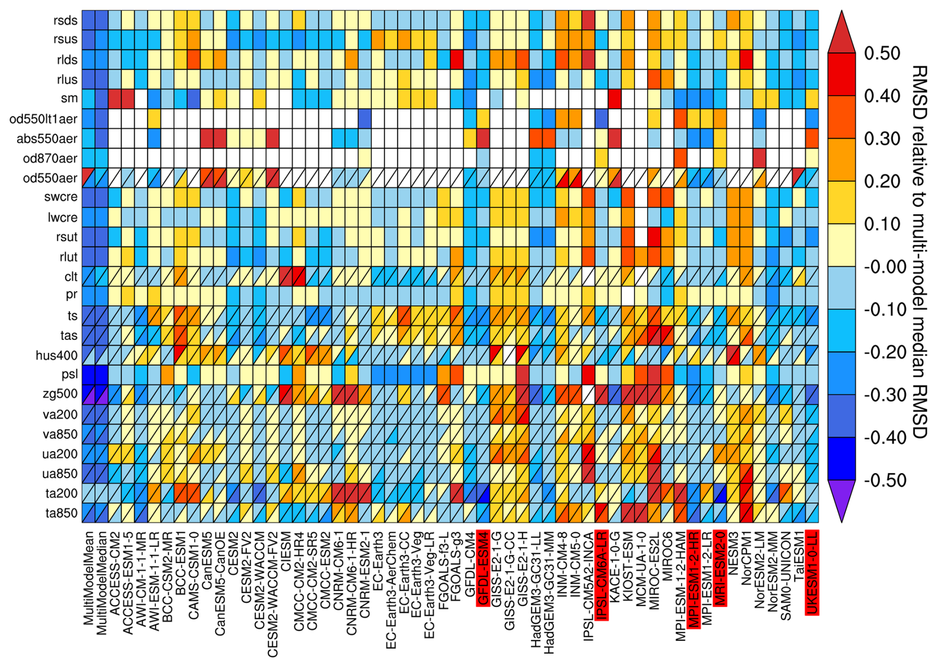
Figure 2 Relative space-time root-mean-square deviation (RMSD) calculated from the climatological seasonal cycle of the CMIP6 historical simulations (1980–1999) compared to observational datasets, for various CMIP6 GCMs (columns) and climate variables (rows), similar to Fig. 6 of Bock et al. (2020). A relative performance is displayed, with blue shading showing better and yellow and red shading showing worse model performance than the median RMSD of all model results of the CMIP6 ensemble. A diagonal split of a grid square shows the relative error with respect to the reference data set (lower right triangle) and an alternative data set (upper left triangle), as listed in Table 5 of Bock et al. (2020). White boxes are used when data are not available for a given model and variable. Models selected for ISIMIP3b are highlighted in red. Variables are (from top to bottom): Surface Downwelling Shortwave Radiation (rsds), Surface Upwelling Shortwave Radiation (rsus), Surface Downwelling Longwave Radiation (rlds), Surface Upwelling Longwave Radiation (rlus), Soil Moisture (sm), Ambient Fine Aerosol Optical Depth at 550 nm (od550lt1aer), Ambient Aerosol Absorption Optical Thickness at 550 nm (abs550aer), Ambient Aerosol Optical Depth at 870 nm (od870aer), Ambient Aerosol Optical Thickness at 550 nm (od550aer), Shortwave Cloud Radiative Effect (swcre), Longwave Cloud Radiative Effect (lwcre), Top-of-Atmosphere Outgoing Shortwave Radiation (rsut), Top-of-Atmosphere Outgoing Longwave Radiation (rlut), Total Cloud Cover Percentage (clt), Precipitation (pr), Surface Temperature (ts), Near-Surface Air Temperature (tas), Specific Humidity at 400 hPa (hus400), Sea Level Pressure (psl), Geopotential Height at 500 hPa (zg500), Northward Wind at 200 hPa (va200), Northward Wind at 850 hPa (va850), Eastward Wind at 200 hPa (ua200), Eastward Wind at 850 hPa (ua850), Air Temperature at 200 hPa (ta200), and Air Temperature at 850 hPa (ta850). Produced with ESMValTool v2.0 (Andela et al., 2020b, a; Righi et al., 2020).

The five GCMs are structurally independent in terms of their ocean and atmosphere model components. Furthermore, all of them have a coupled climate and carbon cycle and in some cases, fully interactive chemistry and aerosol components. We favoured models that applied prognostic couplings between processes and model domains wherever possible to maximise the coverage of simulated feedbacks.

The five GCMs provide a good representation of both the mean and the range of the full CMIP6 multi-model ensemble ECS. According to Meehl et al. (2020), the CMIP6 multi-model mean ECS is 3.7 °C, which is precisely met by the mean ECS of the five ISIMIP3b GCMs. The transient climate response (TCR) of 2.0 °C is also precisely met. This provides an improvement over ISIMIP2b, in the sense of the selected GCM subset reflecting the statistics of the larger CMIP ensemble. In ISIMIP2b the mean ECS for the full CMIP5 was 3.2 °C compared with a mean ECS of 3.72 °C for the four ISMIP2b GCMs (see Tables S1 and S2 in Jägermeyr et al. (2021). The ISIMIP3b ensemble includes three models with below-average ECS (GFDL-ESM4, MPI-ESM1-2-HR, MRI-ESM2-0) and two models with above-average ECS (IPSL-CM6A-LR, UKESM1-0-LL) (see Table 4). In line with their ECS values, we find GFDL-ESM4 and UKESM1-0-LL to project the weakest and strongest global warming, respectively, under any future scenario considered (see Fig. 3). Under SSP5-8.5, the global mean near-surface temperature in 2100 is about 3 °C larger in UKESM1-0-LL than in GFDL-ESM4. Under SSP1-2.6, the projections are about 1.5 °C apart. The ensemble mean warming of the ISIMIP3b CMIP6 models is significantly higher than the warming of the ISIMIP2b CMIP5 models, across global land area by an average of 0.3 °C, but over the main breadbasket cropland regions by more than 0.5 °C between 1983–2013 and 2069–2099, under both SSP1-2.6 and SSP5-8.5 (Table S1 in Jägermeyr et al., 2021). This is in line with the higher median ECS in CMIP6 compared to CMIP5; indeed, some CMIP6 models have an ECS above the assessed likely (2.5 to 4 °C) and very likely (2 to 5 °C) ranges in the IPCC's sixth assessment report (AR6) (Forster et al., 2021). The reasons for these higher estimates of ECS are complex, with cloud feedback processes playing an important role (Zelinka et al., 2020). While the plausibility of the very high ECS estimates has been questioned, recent studies indicate CMIP6 models with high ECS tend to simulate cloud properties better than low ECS models (Bock and Lauer, 2024); also, unaccounted natural variability may have biased the IPCC's assessed ranges somewhat low (Liang et al., 2024; Watanabe et al., 2024).

The ISIMIP3b ensemble reflects the spread in ECS of the overall CMIP6 ensemble, with two models above the AR6 likely range and one of these (UKESM1-0-LL) above the very likely range. The strong warming response of these models should be kept in mind when conducting ISIMIP3b-based impacts studies. However, depending on the region and variable of interest, the high ECS does not necessarily have any bearing on the magnitude or realism of projected regional impacts, and any further selection of models should not be based solely on ECS but on the models' suitability for the impacts variables in question (Swaminathan et al., 2024). In many applications, results can be harmonized by describing the simulated impacts in terms of global mean temperature changes instead of time for the different emission scenarios.

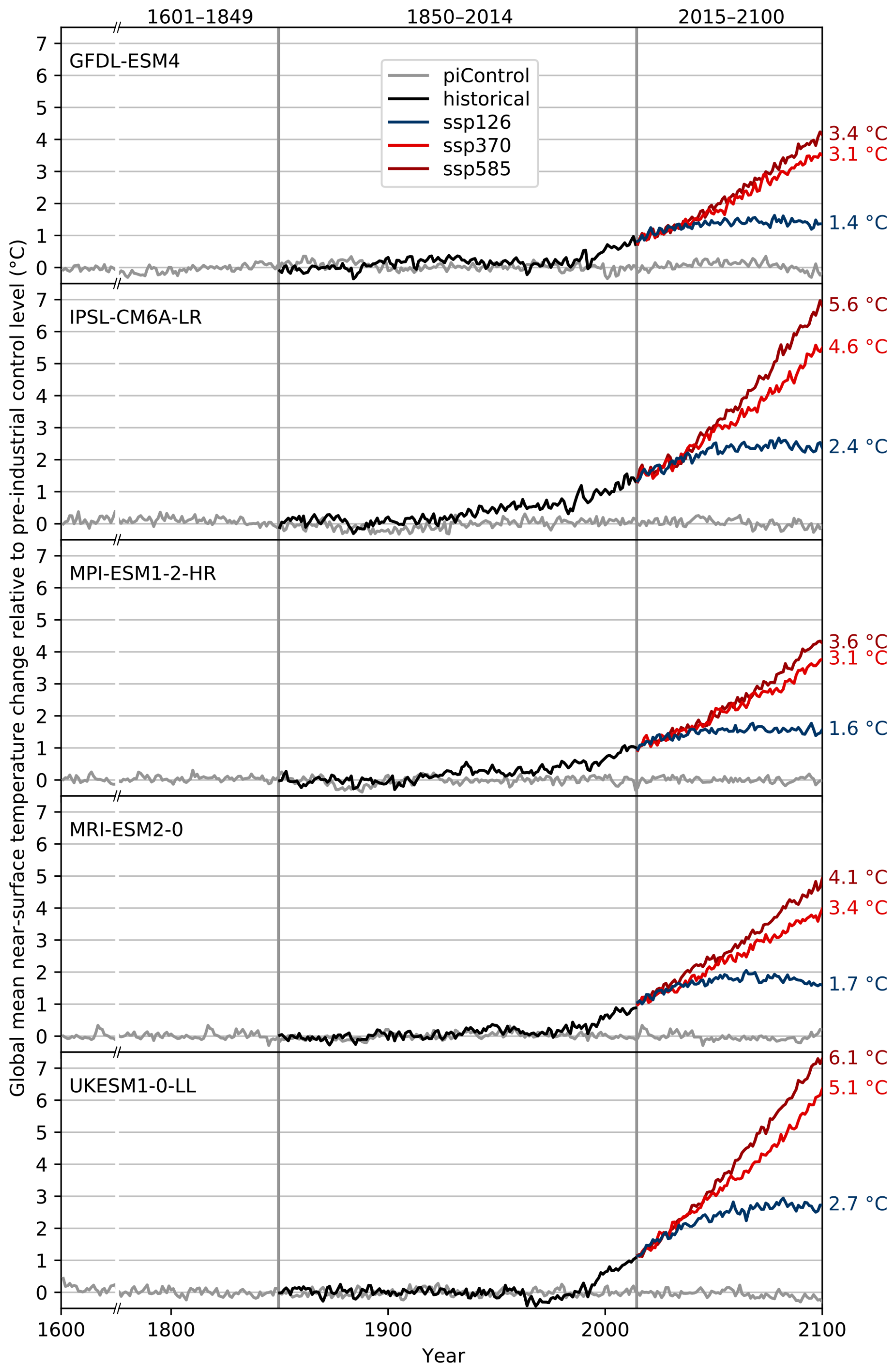
Figure 3 Time series of annual global mean near-surface temperature change relative to pre-industrial levels (1601–1849 average) as simulated with GFDL-ESM4, IPSL-CM6A-LR, MPI-ESM1-2-HR, MRI-ESM2-0 and UKESM1-0-LL (from top to bottom). Colour coding indicates the underlying CMIP6 experiments (grey: pre-industrial control, black: historical, blue: SSP1-2.6, light red: SSP3-7.0, dark red: SSP5-8.5) with corresponding time periods given at the top. Numbers to the right of the plot represent end-of-century warming levels under the different future scenarios, expressed as the global multi-year mean near-surface temperature change from 1601–1849 to 2070–2100.

Bias adjustment and statistical downscaling

To make the GCM-based climate forcing usable for the impact modellers we apply a bias adjustment ensuring that the GCM simulations match the observed distribution of climate data over the historical reference period (1979–2014). In addition to the bias adjustment a statistical downscaling to our standard 0.5° grid is included in the pre-processing of the surface and near-surface atmospheric variables (see Table 3). The method used for the bias adjustment and statistical downscaling (BASD) in ISIMIP3b is version 2.5 of ISIMIP3BASD (Lange, 2019b, 2021a).

ISIMP3BASD has several advantages compared to the method used for bias adjustment and statistical downscaling in ISIMIP2b (Frieler et al., 2017; Lange, 2017, 2018). First, it clearly separates the adjustment of biases in climate model output at 1 or 2° resolution, whatever is closest to the original output data, from the statistical downscaling to the target resolution of 0.5°. Compared to ISIMIP2b, where climate model output was first spatially interpolated to the target resolution and then bias-adjusted, the new approach avoids the associated underestimation of the spatial variability at the target resolution (Lange, 2019b). Second, the new quantile mapping method preserves trends in each quantile of the distribution of the daily data and adjusts biases in distribution quantiles of the daily data more accurately than the ISIMIP2b bias adjustment methods (Lange, 2019b).

For trend preservation, we first produce future pseudo-observations by shifting the historically observed daily data by the simulated future climate change. Here, the signal of climate change is the difference or the ratio between the inverse empirical cumulative distribution function of the historical period and the respective distribution functions of each 36-year period of the future. Using the difference ensures additive trend preservation and using the ratio ensures multiplicative trend preservation under bias adjustment. We apply additive trend preservation for near-surface air temperature (tas), sea level pressure (psl, see Table 3), and surface downwelling longwave radiation (rlds). We apply primarily multiplicative trend preservation for precipitation including snowfall (pr), near-surface wind speed (sfcWind), and the range (tasrange = tasmax − tasmin) between the daily maximum and minimum near-surface air temperatures (tasmax and tasmin, respectively) that can transition smoothly to additive trend preservation for data with large negative biases in the historical period (Lange, 2019b). In a second step, the future simulations are mapped onto the future pseudo-observations by quantile mapping. Both steps, the generation of the future pseudo-observations and the quantile mapping of the future simulations onto the pseudo-observations, are applied for each day of the year separately. The distributions include data from the 31 d around the considered day and all years of the reference or future period, respectively. This means a sample size of 31×36 values for each day of the year. Through this approach the bias adjustment implicitly also adjusts the multi-year mean annual cycle and a mix of year-to-year and day-to-day variability (Haerter et al., 2011).

In addition, the method adjusts the frequency of daily data falling outside of the inner bounds specified in Table 3 (e.g. the dry day frequency, i.e. the number of days with precipitation below 0.1 mm d⁻¹).

Four variables were adjusted and downscaled indirectly: near-surface specific humidity (huss) was derived from adjusted and downscaled near-surface relative humidity (hurs), surface air pressure (ps), and near-surface air temperature (tas) using the equations of Buck (1981) as described in Weedon et al. (2010), snowfall (prsn) was derived from adjusted and downscaled precipitation including snow (pr) and the snowfall ratio (prsnratio = prsn $/$ pr), and daily maximum and daily minimum near-surface air temperatures (tasmax and tasmin, respectively) were derived from adjusted and downscaled tas, and the tasrange = tasmax − tasmin and skewness of the daily temperature cycle tasskew = (tas − tasmin) $/$ (tasmax − tasmin).

The basic characteristics of ISIMIP3BASD (version 1.0) are described in Lange (2019b). However, the method finally used to generate the forcing data now provided within ISIMIP3b (ISIMIP3BASD version 2.5) deviates from the original version in some aspects. In the following we describe the most important updates of the procedure relative to the one described in Lange (2019b). For a complete list of differences between the two versions of the BASD method and the full history of which feature was added in which update, see the CHANGELOG included in the archive of code version 2.5 (Lange, 2021a).

In Lange (2019b) the bias-adjustment was applied on a monthly basis, i.e. the future pseudo-observations and the quantile mapping described above was applied to all daily January data, February data and so forth. This approach can introduce discontinuities at the transition from one month to another (see Fig. 4). That is why for ISIMIP3b the adjustment is done in the running window mode with steps of 1 d and a window width of 31 d as described above. This approach resolves the discontinuity issue (see Fig. 4), as suggested by Themeßl et al. (2012) Thrasher et al. (2012) Gennaretti et al. (2015) and Grenier (2018).

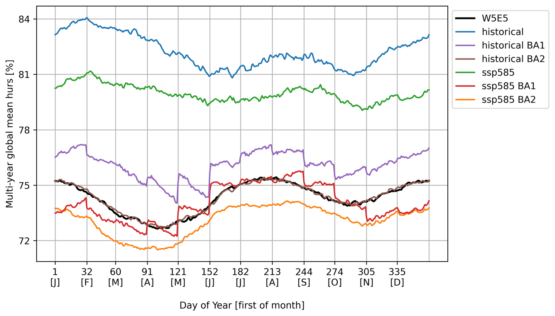
Figure 4 Global multi-year daily mean near-surface relative humidity for UKESM1-0-LL historical (1979–2014) and SSP5-8.5 (2065–2100), with uncorrected historical simulated data in blue, uncorrected future simulated data in green, historical bias-adjusted data in purple and brown, future bias-adjusted data in red and orange, and observational reference data in black. The bias is effectively reduced throughout all days of the year (brown line closely matching the black line) when ISIMIP3BASD v2.5 is applied in running-window mode in steps of 1 d (BA2). In contrast, a month-by-month application, which was the only option in ISIMIP3BASD v1.0, generates discontinuities at each turn of the month (BA1).

Since ps, rlds and tas can show significant trends within the 36-year training and application periods ISIMIP3BASD v1.0 includes a detrending of these variables within these intervals before the pseudo-future observations and the transfer functions are estimated and applied. Afterwards the trend is added back again. This is done to prevent the confusion of trends with interannual variability during quantile mapping (Lange, 2019b; Maraun, 2013). In contrast to v1.0, in v2.5, applied to generate the ISIMIP3b forcing data, the detrending is only applied if the trend is significantly different from zero at the 5 % level.

We also changed the method used to generate future pseudo-observations of bounded variables (Eqs. 8 and 9 of Lange, 2019b), in order to stabilise results in some edge cases. If, e.g., the historically observed relative dry-day frequency was 0.0 while the simulated frequency was 0.8 for the historical period and 0.9 for some future period, then, according to Eq. (9) of Lange (2019b), the future pseudo-observed frequency would be equal to $\mathrm{1}-(\mathrm{1}-\mathrm{0.0})(\mathrm{1}-\mathrm{0.9})/(\mathrm{1}-\mathrm{0.8})=\mathrm{0.5}$. As this is considered unrealistic we apply a revised version of Eq. (9) of (Lange, 2019b) that reads

$$\begin{array}{}\text{(1)}& P_{\mathrm{fut}}^{\mathrm{obs}}=\left\{\begin{array}{l}{P}_{\mathrm{fut}}^{\mathrm{sim}}\text{ if }\\ P_{\mathrm{hist}}^{\mathrm{sim}}=P_{\mathrm{hist}}^{\mathrm{obs}},\\ \mathrm{0}+(P_{\mathrm{hist}}^{\mathrm{obs}}-\mathrm{0})(P_{\mathrm{fut}}^{\mathrm{sim}}-\mathrm{0})/(P_{\mathrm{hist}}^{\mathrm{sim}}-\mathrm{0})\\ \text{if }{P}_{\mathrm{fut}}^{\mathrm{sim}}\le P_{\mathrm{hist}}^{\mathrm{sim}}>P_{\mathrm{hist}}^{\mathrm{obs}},\\ \mathrm{1}-(\mathrm{1}-P_{\mathrm{hist}}^{\mathrm{obs}})(\mathrm{1}-P_{\mathrm{fut}}^{\mathrm{sim}})/(\mathrm{1}-P_{\mathrm{hist}}^{\mathrm{sim}})\\ \text{if }{P}_{\mathrm{fut}}^{\mathrm{sim}}\ge P_{\mathrm{hist}}^{\mathrm{sim}}<P_{\mathrm{hist}}^{\mathrm{obs}},\\ P_{\mathrm{hist}}^{\mathrm{obs}}+P_{\mathrm{fut}}^{\mathrm{sim}}-P_{\mathrm{hist}}^{\mathrm{sim}}\text{ otherwise}.\end{array}\right.\end{array}$$

In this revised relation, the otherwise case applies if $P_{\mathrm{fut}}^{\mathrm{sim}}<P_{\mathrm{hist}}^{\mathrm{sim}}<P_{\mathrm{hist}}^{\mathrm{obs}}$ or $P_{\mathrm{fut}}^{\mathrm{sim}}>P_{\mathrm{hist}}^{\mathrm{sim}}>P_{\mathrm{hist}}^{\mathrm{obs}}$. Hence it applies to the aforementioned edge case, where it produces a less extreme future pseudo-observed relative frequency of $\mathrm{0.0}+\mathrm{0.9}-\mathrm{0.8}=\mathrm{0.1}$. Equation (8) of Lange (2019b) was revised analogously to Eq. (9).

Furthermore, we refined the method used to generate future pseudo-observations (step 5 of the bias adjustment algorithm of Lange, 2019b) for all variables with at least one bound: In v1.0, the future pseudo-observations were generated by transferring simulated trends in all distribution quantiles to the observational reference data. That included trends in, e.g., precipitation quantiles below the wet-day threshold. However, in some cases, the trend transfer turned many dry days into wet days, with a profound impact on the shape of the distribution of future pseudo-observed wet-day precipitation. As a result, simulated trends in wet-day precipitation intensity were not well preserved. In v2.5, trend transfers are restricted to values within threshold. This particularly improves the preservation of trends in wet-day precipitation intensities.

We also modified the bias adjustment method for Near-Surface Relative Humidity (hurs) because ISIMIP3BASD v1.0 turned out to produce unrealistic distributions of hurs under climate change if there are too many cases of supersaturation (hurs ≥100 %) in the simulated data. This is the case for several of the CMIP6 GCMs selected for ISIMIP3b, particularly in high-latitude winter: While no supersaturations are found in the observational reference data, the GCM simulates many supersaturations in the historical reference period and even more so in a future period, under SSP5-8.5 (see Fig. 5). ISIMIP3BASD v1.0 preserves this projected trend and hence produces future bias-adjusted hurs data with many supersaturations. In v2.5, this trend is no longer preserved. Instead, the supersaturation probability is fixed at the observed level, which is zero or very close to zero in all seasons and grid cells for W5E5. Future pseudo-observations of hurs are generated by applying the revised (see above) Eq. (8) of Lange (2019b) to all hurs values after capping them at 100 %. The new approach was motivated by findings from Ruosteenoja et al. (2017, 2018). They analysed hurs data from CMIP5 and showed that (i) supersaturations in those data are mostly spurious, resulting from, e.g., inconsistencies in the interpolation of temperature and specific humidity to the near-surface level, and (ii) climatological mean value trends of hurs become more consistent with trends in relative humidity from the lowest model level if hurs is capped at 100 % before trends are calculated.

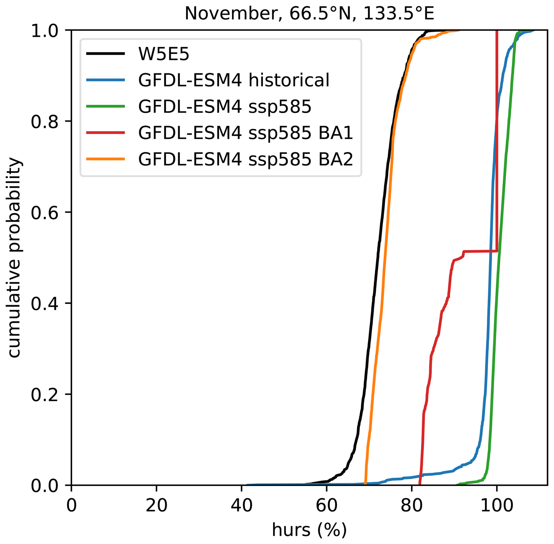
Figure 5 Empirical cumulative distribution functions of near-surface relative humidity in high-latitude winter (November, 66.5° N, 133.5° E) for GFDL-ESM4 historical (1979–2014) and SSP5-8.5 (2065–2100), with historical simulated data in blue, future simulated data in green, future bias-adjusted data in red and orange, and observational reference data in black. The simulated climate change signal is well preserved with ISIMIP3BASD v2.5 using a fixed supersaturation (hurs ≥100 %) probability and Eq. (1) applied to all hurs values after capping them at 100 % to generate future pseudo-observations (orange, BA2). In contrast, the simulated climate change signal is not well preserved if the supersaturation probability is allowed to change and Eqs. (8) and (9) of Lange (2019b) are used to generate future pseudo-observations of hurs (red, BA1).

In addition, while ISIMIP3BASD v1.0 applies parametric quantile mapping to all climate variables, we used a nonparametric approach for the bias adjustment of near-surface relative humidity (hurs), the snowfall ratio (prsnratio), surface downwelling shortwave radiation (rsds), and the skewness of the daily temperature (tasskew) since the parametric quantile mapping method previously used for those variables suffered from occasionally unstable beta distribution fits.

Moreover, the parametric quantile mapping described in Lange (2019b) does not only adjust biases in quantiles of the simulated daily data but also adjusts biases in the likelihood of individual events, as in Switanek et al. (2017). To avoid overfitting artifacts we did not adjust event likelihoods for ISIMIP3b.

Finally, the diurnal temperature range (tasrange) was ultimately bias-adjusted using a Weibull distribution, not a Rice distribution as described in Lange (2019b) because the Weibull distribution fits the data better in most cases, in particular in the upper tail.

For further details of the application of ISIMIP3BASD v2.5 for ISIMIP3b, including the exact Python commands and application periods used per CMIP6 experiment, see the ISIMIP3b bias adjustment fact sheet (Lange, 2021b).

In addition, we use a new observational target dataset. Instead of using the EWEMBI dataset (E2OBS, WFDEI and ERAI data merged and bias-corrected for ISIMIP; (Lange, 2019a)) in ISIMIP3b we adjust the climate forcing data to version 2.0 of the W5E5 dataset (WFDE5 over land merged with ERA5 over the ocean; Lange et al., 2021). The data cover the entire globe at 0.5° horizontal and daily temporal resolution from 1979 to 2019. W5E5 v2.0 is derived by applying version 2.0 of the WATCH Forcing Data methodology (WFDE5; Cucchi et al., 2020) to ERA5 reanalysis data (Hersbach et al., 2020) and precipitation data from version 2.3 of the Global Precipitation Climatology Project (GPCP; Adler et al., 2003).

The statistical downscaling method did not change between v1.0 and v2.5 of ISIMIP3BASD, i.e. for ISIMIP3b we use the approach described by Lange (2019b). This method adds the spatiotemporal variability that is missing at the low spatial resolution at which the bias adjustment is done (1 or 2°, depending on the GCM), compared to the target resolution of the downscaling (0.5°). The method is a modified version of the MBCn algorithm from Cannon (2018), which in turn is a stochastic, multivariate, non-parametric quantile mapping method. We use it to transfer the statistical relationship between low-resolution and high-resolution W5E5 data to the GCM output that was previously bias-adjusted using low-resolution W5E5 data. In comparison to the approach used in ISIMIP2b (a spatial interpolation to the target resolution followed by a bias adjustment at that resolution), the approach used in ISIMIP3b is less prone to inflate temporal variability and deflate spatial variability, i.e. the ISIMIP3b approach produces more realistic spatiotemporal variability patterns at the target resolution (Lange, 2019b).

Table 5 Information about tropical cyclone tracks and windfields provided as climate-related forcing data within ISIMIP3b. Variable specifiers are set in bold.

3.2 Tropical cyclones

We provide large ensembles of potential realisations of TC tracks and intensities that are consistent with the large-scale atmospheric and oceanic conditions simulated by four of the five ISIMIP3b GCMs (see Table 6) and for a selection of scenarios considered in ISIMIP3b (see Table 1). The tracks are generated by two different statistical-dynamical approaches, the MIT approach and the CHAZ approach detailed below, forced by data from the ISIMIP3b GCMs listed in Table 6. For the MIT approach, we provide gridded wind (maximum 1 min sustained wind speeds during the whole duration of the TC) and rainfall (maximum 24-hourly amounts of rain during the whole duration of the TC) fields at a spatial resolution of 300 arcsec (approximately 10 km) using the same approaches also applied to the historically observed tracks (Frieler et al., 2024), Sect. 4.2).

Both methods to generate the TC tracks are assessed in Meiler et al. (2025). The modeling approaches consist of a genesis, a track, and an intensity module:

MIT approach. Within MIT (Emanuel et al., 2008), the time-evolving state of the atmosphere and ocean surface given by the GCMs is randomly (uniformly distributed in time and space) seeded by weak proto-cyclones (genesis module). The seed disturbances are assumed to move with the GCM-provided large-scale flow in which they are embedded, plus a westward and poleward component owing to planetary curvature and rotation (track module). Their intensity is calculated using the Coupled Hurricane Intensity Prediction System (CHIPS; Emanuel et al., 2004), a simple axisymmetric hurricane model coupled to a reduced upper ocean model to account for the effects of upper ocean mixing of cold water to the surface (intensity module). Applied to the synthetically generated tracks, this model simulates which of the seeded proto-cyclones develop into TCs, reaching maximum 1 min sustained wind speeds of at least 35 knots, or dissipate due to unfavourable environments. The probabilistic seeding of proto-cyclones is repeated until the desired number of storms per year is reached (in our case, 1500). For each year, the share of proto-cyclones that dissipated in the process is used to derive an estimate of annual TC occurrences (freqyear). Extensive comparisons to historical events (Emanuel et al., 2008) have revealed that the statistical properties of the simulated events are consistent with historical TC genesis.

For each year of the ISIMIP3b period 1850—2100 (except for GFDL-ESM4, where tracks were only generated for 1850–2014 and 2061–2100, and MRI-ESM2-0 for 1950–2100, see Table 1), 1500 tracks were generated, globally. Depending on the application, a simple subsampling (Meiler et al., 2022) or a more advanced bias-correction and emulation procedure (Geiger et al., 2021) might be necessary to extract properly-sized sets of potential realisations from the MIT ensembles.

The “ISIMIP3b tropical cyclone tracks MIT” dataset shall only be used for noncommercial purposes, including teaching and research at universities, colleges and other educational institutions, research at non-profit research institutions, and personal non-profit purposes. It is accessible through the ISIMIP data portal (https://data.isimip.org/access/ISIMIP3b/InputData/climate/tropical_cyclones/MIT/tracks/, last access: 20 December 2025) after agreeing to the corresponding license.

For using the tracks for commercial purposes, including but not restricted to consulting activities, software or data products, and a commercial entity participating in research projects, please contact Kerry Emanuel (MIT, email: emanuel@mit.edu) for an appropriate license.

CHAZ approach. CHAZ (Lee et al., 2018) seed disturbances are also initialised randomly, but, in contrast to the MIT model, the global seeding rate and the local probabilities are derived from two versions of a TC genesis index (TCGI, Tippett et al., 2011 (genesis module)) and intended to represent the environmental conditions instead of being adjusted to produce a prescribed number of TCs. It is noted that CHAZ's projection of global and basin-wide TC annual frequency is sensitive to the choice of the particular variable used to represent moisture in its genesis module. Simulations using column relative humidity (CRH) as the moisture variable tend to project an overall increase in global TC frequency, while those using saturation deficit (SD) show a decrease (Camargo et al., 2014; Lee et al., 2020). Both parameters describe how far the atmosphere is from saturation, and they have very similar spatial patterns in the present climate, so historical data cannot be used to determine which variable is the best choice to represent the climate. These two configurations reflect the uncertainty of TC frequency projections (Sobel et al., 2021). Here we provide CHAZ downscaling using both choices of moisture variable to account for this uncertainty.

Similar to MIT, CHAZ then moves the synthetic storms by advection of the environmental steering flow plus a beta drift (track module). The evolution of synthetic storm intensity is calculated using the surrounding atmospheric conditions through an empirical multiple linear regression model plus a stochastic component (intensity module, Lee et al., 2015, 2016). The stochastic component accounts for internal storm dynamics that do not depend explicitly on the environment. While, in MIT, TC occurrence frequency is provided as an additional variable, in CHAZ, this information is implicitly contained in the number of TCs that were seeded by the genesis module and that reached TC strength according to the intensity module.

For ISIMIP3b, 20 different CHAZ realisations of the genesis and subsequent tracks are generated with 40 ensemble members each from the intensity module for the historical period and for all RCP-SSP combinations considered within ISIMIP3b. For each of the 20 realisations, we compute wind and rain fields for the first ensemble member from the intensity ensemble. The design of 20 realisations allows CHAZ to generate similar numbers (∼1800) of synthetic storms per year per GCM as the MIT models over the historical period. The exact number of storms per year in CHAZ varies by GCM, by scenario, by the choice of humidity variables in CHAZ's genesis component (Lee et al., 2020). On average, CHAZ generates 1817, 1802, 1820, 1810, 1842 storms per year for GFDL-ESM4, IPSL-CM6A-LR, MPI-ESM1-2-HR, MRI-ESM2-0, and UKESM1-0-LL, respectively. The CHAZ model has been shown to capture the statistical properties of the observed storms when forced by global reanalysis data (Lee et al., 2018). Its CMIP6 downscaling results are reported in Fosu et al. (2024). Sobel et al. (2019) used both models to study cyclone risk for Mumbai, India and showed that MIT and CHAZ generate comparable return periods (frequency of exceedance) of maximum wind speeds at landfall. However, a frequency bias-correction might still be necessary, depending on the application (Meiler et al., 2022).

The “ISIMIP3b tropical cyclone tracks (CHAZ)” dataset shall only be used for noncommercial purposes, including teaching and research at universities, colleges and other educational institutions, research at non-profit research institutions, and personal non-profit purposes. It is accessible through the ISIMIP data portal (https://data.isimip.org/access/ISIMIP3b/InputData/climate/tropical_cyclones/CHAZ/tracks/, last access: 6 March 2026) after agreeing to the corresponding license.

For using the tracks for commercial purposes, including but not restricted to consulting activities, software or data products, and a commercial entity participating in research projects, please contact Chia-Ying Lee (Columbia University, email: cl3225@columbia.edu) for an appropriate license.

Table 6 Climate input data interpolated to 2° horizontal resolution and provided without bias adjustment for tropical cyclone modelling with MIT and CHAZ. Variable specifiers are set in bold.

3.3 Coastal water levels

We do not yet provide coastal water levels as forcing data for ISIMIP3b. However, we plan to generate time series of coastal water levels from 1900 to 2100 at hourly resolution or for daily maxima. The data set and method will be described in a separate manuscript. Similar to the hourly water level dataset of ISIMIP3a (see Sect. 3.3 of Frieler et al., 2024, and Treu et al., 2024), we will combine long-term annual sea level change with estimates of short-term coastal water level variation. Concerning the long-term sea level change component, we go beyond the ISIMIP2b approach (Frieler et al., 2017) and use tide gauge, satellite, vertical land motion and global climate model data to constrain a model with observations and IPCC AR6 projections in a Bayesian setting building on Perrette and Mengel (2025). The Perrette and Mengel (2025) model allows for smooth projections of relative sea level from observational time series collected at tide gauge stations with an explicit representation of the different components of sea level rise. To become usable for ISIMIP3 we will (a) extend the approach to all coastlines and (b) use GCM output directly for the global thermosteric and local sterodynamic components (Gregory et al., 2019) of sea level rise, which are modeled by the GCMs. Extension to all coastlines is possible for the ice sheet, glacier and sterodynamic components as they rely on spatial fingerprints or GCM output. Processes driving vertical land motion that are not related to large scale climate processes are however more difficult to model. They are estimated from data as residual vertical land motion in Perrette and Mengel (2025). As we do not have data at all coastlines we will extrapolate in time and space the historical rates from tide gauge sites or apply zero rates for this component. Using the explicit component structure of the model, the method will provide relative sea level projections (including vertical land motion), which can be directly used in coastal impact studies. We plan to estimate the short-term coastal water level variation by a machine-learning approach that is trained to reproduce simulations of the Global Tide and Surge Model (GTSM) driven by ERA5 reanalysis data (Muis et al., 2020) or simulations from HighResMIP (Muis et al., 2023). We are currently testing the dependency of the short-term water level variation on available atmospheric information at GCM resolution. If the predictive power is high enough we will use the findings to provide computationally efficient water level projections specific for the ISIMIP GCMs.

Table 7 Coastal water level specifications. Variable specifiers are set in bold.

3.4 Ocean data

In the default experiments, the ocean variables provided by the GCMs are not subject to bias-adjustment, unlike the atmospheric forcing data (Sect. 3.4.1). This is due to the absence of a comprehensive global observational oceanic dataset to serve as a reference for the adjustment.

However, in order to mitigate potential biases in global impact model simulations stemming from biases in raw oceanic forcing data, we plan to provide a de-biased version to be used in a sensitivity experiment (see Table 2). They will be derived from an ocean-biogeochemistry model forced by bias-adjusted monthly atmospheric surface flux data from four of the five ISIMIP3b GCMs. The approach preserves the monthly variability of the underlying GCM while the daily variability is added from an independent simulation (see Sect. 3.4.2).

For the regional impact model simulations, observational data for individual variables have either been applied directly (if the required forcing was observed) to rectify biases in regional oceanic forcings by the delta method or have first been translated into the required forcing variable by model simulations (see Sect. 3.4.3). The regional bias-adjustment is independent from the generation of the global de-biased forcing data.

In order to gauge the effects of these adjustments on the corresponding impact simulations, the protocol includes sensitivity experiments (“de-biased”) grounded on these adjusted CRF (see Table 2). The comparison of associated impact simulation to the default ones is expected to provide valuable insights into the effects of potential biases in the CRF. The “de-biased” experiments are considered a starting point to develop methods to bias-adjust the oceanic forcings in further ISIMIP simulation rounds and make these simulations the default ones. Following the ISIMIP “consistency framing” the bias-adjustment should also preserve the daily variability of the original GCM simulations to allow for a cross-sectoral integration on daily time scale.

3.4.1 Raw data without bias adjustment (default experiment)

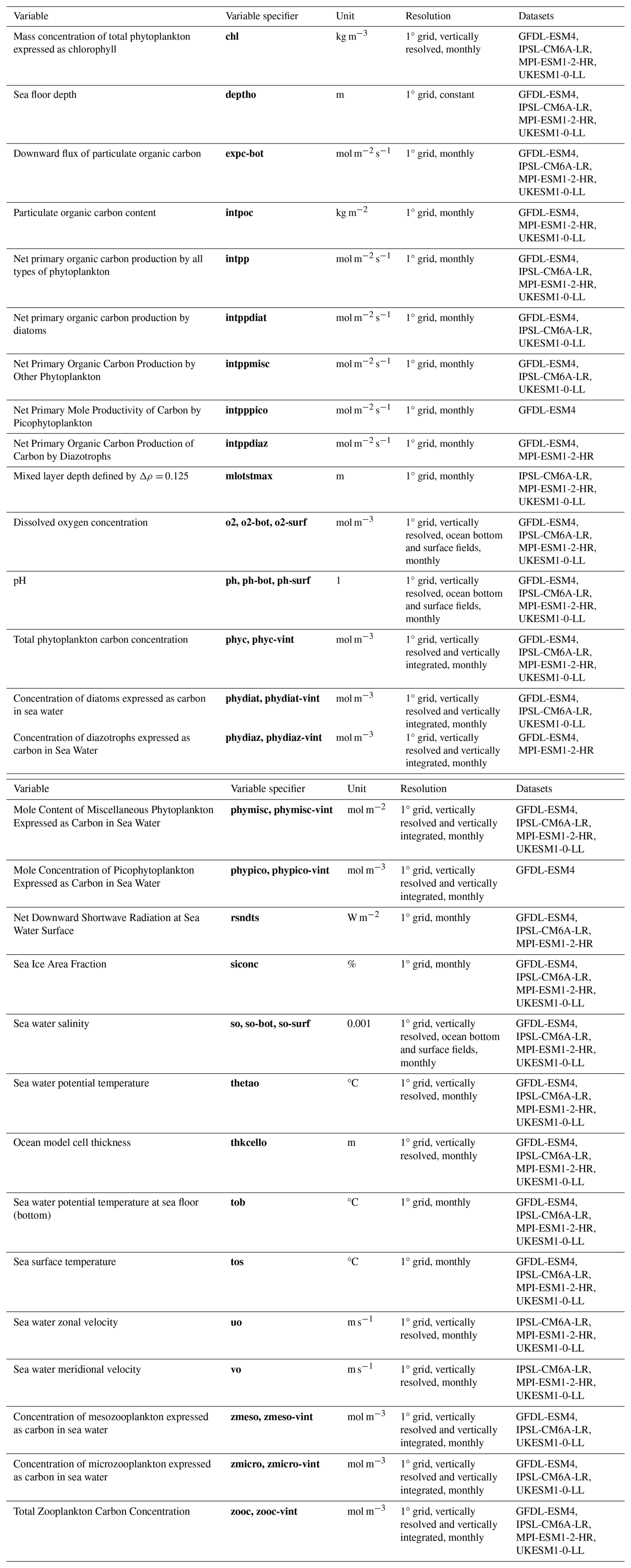
In ISIMIP3b, a set of physical and biogeochemical ocean variables nearly identical to that in ISIMIP3a is provided (see Sect. 4.4, Table 8 of Frieler et al., 2024, and Table 8 below). These variables are obtained from the CMIP6 GCMs, which also supply the atmospheric forcing for ISIMIP3b, except for MRI-ESM2-0, which lacks bio-geochemical variables. In other models, only certain individual variables are missing (see Table 8). Obtaining both atmospheric and oceanic variables from the same set of GCMs ensures consistency between the fisheries and marine ecosystems sector and other ISIMIP sectors. The available variables in ISIMIP3b are interpolated from the native grids of the ocean models to a regular 1° grid. This resolution is comparatively lower than that of the ISIMIP3a ocean input data due to the generally reduced native resolution of CMIP6 GCM simulations compared to the ocean model used to generate the oceanic forcings based on observational atmospheric forcings for ISIMIP3a.

Table 8 Oceanic climate-related forcing data provided within ISIMIP3b. Variables with suffixes -bot, -surf, and -vint were obtained from the seafloor, the top layer of the ocean, and vertical integration, respectively. Variable specifiers are set in bold.

3.4.2 Bias-adjusted global ocean forcings (“de-biased” sensitivity experiment)

GCMs have been shown to have limitations in accurately representing various aspects of the present climate system (Eyring et al., 2023), (Séférian et al., 2020), that are also expected to affect regional physical and biogeochemical oceanic projections (Li et al., 2016), (Tagliabue et al., 2021). In particular, biases in sea-surface temperature (SST, variable “tos”) and nutricline as well as thermocline depth influence oceanic primary productivity, which in turn has major influence on various marine ecosystem processes. Thus, reducing the substantial biases in GCMs' ocean variables through bias-adjustment is desirable. Typically, for bias-adjustment of atmospheric variables, statistical approaches are used where a transfer function is trained to map the simulated historical distribution of the relevant variables to the observed distribution and then applied to future simulations. Yet for oceanic variables, the scarcity of comprehensive sub-surface observational data globally does not allow for a similar, direct adjustment of the relevant variables. However, standalone ocean-biogeochemistry simulations, when driven by observation-based atmospheric reanalysis data, have been demonstrated to considerably alleviate SST-related biases and typically provide satisfactory simulations of the physical ocean and marine biogeochemistry for the historical period (e.g. Tsujino et al., 2020; Barrier et al., 2023). Thus, an alternative process-oriented bias-adjustment approach has been developed that relies on a comprehensive ocean-biogeochemistry model that is forced by bias-adjusted atmospheric forcings. The adjustment of the ISIMIP3b oceanic forcings builds on such a dynamical de-biasing approach (Lengaigne et al., 2025), which relies on conducting forced oceanic simulations using the NEMO-PISCES physical-biogeochemical ocean model (Madec, 2015), which is the oceanic component of the IPSL-CM6A-LR climate model. The ocean model needs to be forced with high-frequency (3-hourly) surface momentum, heat and freshwater fluxes. Since from the CMIP6 pre-industrial, historical, and future scenario simulations used in ISIMIP3b these variables are only available at monthly resolution, additional steps are necessary to generate climatological high-frequency fluxes first. In the following, we first describe these preparatory steps, and then the de-biasing strategy, in more detail.

Table 9 Bias-adjusted ocean data to be used by global impact models in the “de-biased” sensitivity experiment in the fisheries and marine ecosystems sector. Variable specifiers are set in bold.

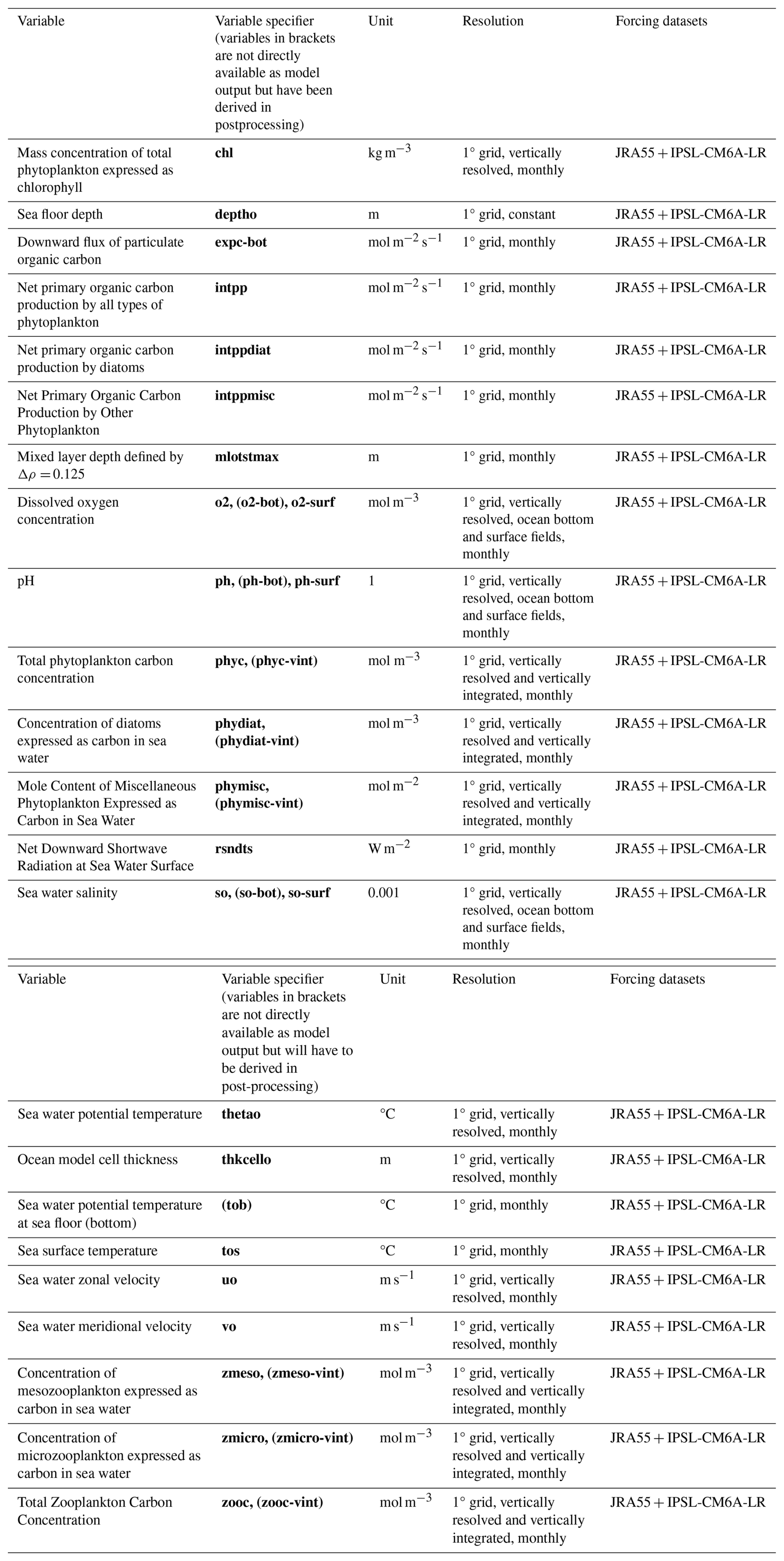
High-frequency surface flux forcing. Initially, a climatological simulation spanning the historical period from 1958 to 2022 is performed by forcing the ocean model NEMO-PISCES with a single repeating annual cycle representative of the 1990s' climate conditions sourced from the “Repeat Year Forcing” (RYF) from JRA55 reanalysis (Stewart et al., 2020). This simulation is driven using the CORE bulk formulae (Large, 2004), incorporating all surface atmospheric variables at 3-hourly resolution from JRA55 RYF as inputs and storing 3-hourly momentum, heat and freshwater fluxes from this simulation. These 3-hourly JRA55 RYF fluxes are then added to the monthly seasonal flux anomalies available from the ISIMIP3b climate models for the pre-industrial (picontrol), historical (historical) and future SSP1-2.6 (ssp126), SSP3-7.0 (ssp370), and SSP5-8.5 (ssp585) scenarios. In this way, 3-hourly surface flux forcings are created for all ISIMIP3b scenarios. Notably, this procedure results in sub-monthly variability mirroring that of the JRA55 RYF, rather than the variability simulated by the coupled climate model. This means that any projected changes in sub-monthly variability due to climate change are not integrated in the final de-biased product. However, to date, marine ecosystem modellers have not analysed sub-monthly variability anyways (and most marine ecosystem models are not suited to account for sub-monthly variability of forcings), making this approach suitable.

Alternatively, de-biased ocean simulations including GCM-based sub-monthly variability could be constructed by an alternative approach. In this scenario, 3-hourly surface atmospheric variables would be extracted directly from each GCM simulation, rather than from JRA55 RYF forced oceanic simulations. Forcing NEMO-PISCES with these variables using bulk formulae would once again produce the necessary 3-hourly surface fluxes, this time with variability consistent with the coupled GCM across all timescales. This approach however requires running a separate ocean simulation for each GCM and scenario to derive the surface fluxes, necessitating a much larger number of ocean model runs than the approach using JRA55 RYF. In addition, the 3-hourly input from the GCMs is not available for all scenarios.

De-biasing strategy. The 3-hourly surface fluxes, constructed as described above, then serve as input for another set of NEMO-PISCES ocean model simulations which produce the final, bias-adjusted historical and future forcings for the marine ecosystem models. Since these ocean model simulations are driven directly with surface fluxes (instead of bulk formulae), they enable an online implementation of the surface heat flux feedbacks triggered by climate change, which is important for realistically representing the effects of global warming (Lengaigne et al., 2025). As described by Lengaigne et al. (2025), climate change alters surface fluxes both directly through the effect of greenhouse gases on atmospheric characteristics, such as wind speed or humidity; and through feedback effects related to changes in SST. For our bias-adjustment procedure, to maintain physical consistency, the part of the anomalous surface fluxes that directly depends on climate change-induced SST warming is separated from the part that does not. Only the latter part is used as a direct flux input to NEMO-PISCES, while the former is implemented within NEMO-PISCES as an online relaxation to the warming signal from the debiased historical and future simulations using a spatially and seasonally variable feedback damping coefficient. This SST feedback coefficient, derived from observed surface variables, represents the Newtonian cooling negative feedback related to latent heat fluxes through the Clausius-Clapeyron relationship and the negative feedback related to upward long-wave radiation through Stefan's law (Zhang and Li, 2014) and the positive downward longwave radiation feedback related to increasing temperature (Shakespeare and Roderick, 2022). Application of this approach to the NEMO-PISCES ocean model effectively reproduces the global SST changes simulated by CMIP6 models, as demonstrated in Lengaigne et al. (2025).

In this way, physical and biogeochemical ocean simulations are generated for picontrol and historical climate forcings as well as for each of the future climate change scenarios, ensuring that the background climatological state is constrained by the reanalysis, while still accounting for both interannual and long-term climate variability simulated by the underlying GCM. Consequently, the resulting ocean-biogeochemistry simulations considerably mitigate the strong present-day climatological biases identified in the coupled models. Depending on data availability for the relevant monthly fluxes, this de-biasing procedure can be applied to any climate model. The set of variables included in the de-biased dataset will be a subset to the one in the raw GCM dataset (Table 8), detailed in Table 9.

Additionally, to generate observation-based oceanic forcings for ISIMIP3a, a reference simulation is also forced with the full JRA55 forcing (Tsujino et al., 2018) that includes observed inter-annual and decadal variability. This oceanic forcing is expected to be a valuable additional CRF for impact model evaluation within ISIMIP3a akin to the GFDL-MOM6-COBALT2 reanalysis-driven historical dataset used in ISIMIP3a (Frieler et al., 2024).

3.4.3 Bias-adjusted regional ocean forcings (“de-biased” sensitivity experiment)

Regional marine ecosystem models are most often calibrated to reproduce observed environmental variables when driven by observed sea surface and bottom temperature, primary production (phytoplankton production), and zooplankton biomass. However, despite this calibration, biases may still occur in the ecosystem model's historical simulations when it is forced by – potentially biased – climate model data instead of observational data. To reduce this effect the GCM-based input data has been adjusted such that the historical GCM simulations match observational data for certain regions (Eddy et al., 2025). The adjustment is based on the delta approach where simulated and observational forcing data X_sim and X_obs are averaged across a given historical reference period to determine the bias Δ = mean (X_sim) − mean (X_obs) that is then subtracted from the simulated forcing data. This method preserves the trend in the forcing data and its internal variability. Some ocean forcing variables are not an exact match with variables used in regional marine ecosystem models. For example, sea water potential temperature (thetao), concentration of diatoms (phydiat-vint), or concentration of mesozooplankton (zmeso-vint) may first be converted to other indicators that are then used as input for the regional marine ecosystem models. In these cases the derived indicator is corrected using the delta method (see Table 10).

Table 10 Bias-adjusted ocean data to be used by regional impact models in the “de-biased” sensitivity experiment in the fisheries and marine ecosystems sector. EwE: Ecopath with Ecosim. See Ortega-Cisneros et al. (2025) for details about this and other ecosystem models mentioned. Variable specifiers are set in bold.

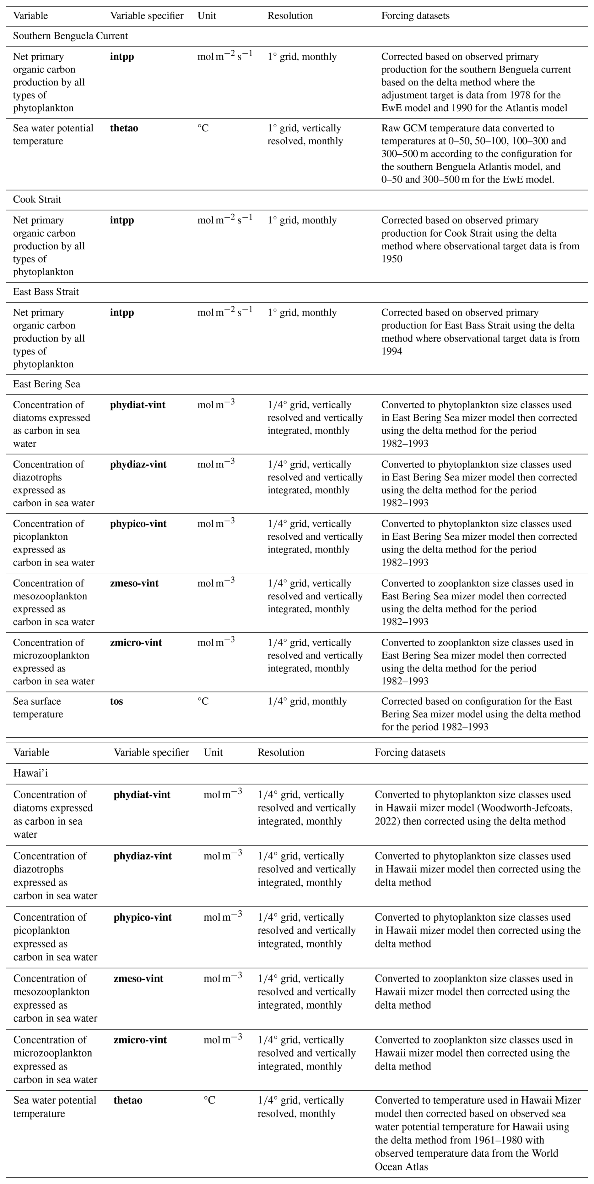
3.5 Future Lightning Data

For the “varlightning” sensitivity experiment we provide temporally varying lightning density (strokes km⁻² d⁻¹) for the period 2015–2100 on monthly resolution (monthly mean of daily lightning stroke density) and the standard 0.5° global grid. This dataset may be used in a range of applications, for example, to understand the influence of lightning on wildfire ignition or atmospheric composition.

The lightning density is derived from future climate simulations of UKESM1-0-LL and an empirical relationship between Convective Available Potential Energy (CAPE) and lightning strokes based on the WWLLN Global Lightning Climatology and time-series (WGLC) (Kaplan and Lau, 2021, 2022). Daily mean CAPE is calculated from non bias-adjusted air temperature, air pressure, and specific humidity on pressure levels from the surface to the top of the troposphere.

The relationship between daily CAPE and daily lightning is estimated by linear regression of log-transformed CAPE derived from the GCM-calculated CAPE during the period of overlapping model output and observed daily lightning from WGLC (2015–2020) for each gridcell and month of the year. Where <10 observations of daily lightning are available over the calibration period, we use global mean regression parameters.

The empirical relationships are applied to the daily CAPE data from the UKESM1-0-LL simulations for all three climate scenarios SSP1-2.6, SSP3-7.0, and SSP5-8.5. The associated lightning densities were monthly averaged. To maintain the spatial structure of lightning observed at present, lightning anomalies compared to the simulated 2015–2020 climatological reference were added to the observed present-day lightning climatology from WGLC for 2015–2020. The “varlightning” sensitivity experiment is assumed to start from the default historical group I simulation, assuming the Flash Rate Monthly Climatology (Cecil, 2006), not changing with climate change.

Table 11 Future lightning forcing data provided within ISIMIP3b. Variable specifiers are set in bold.

4 Conclusions

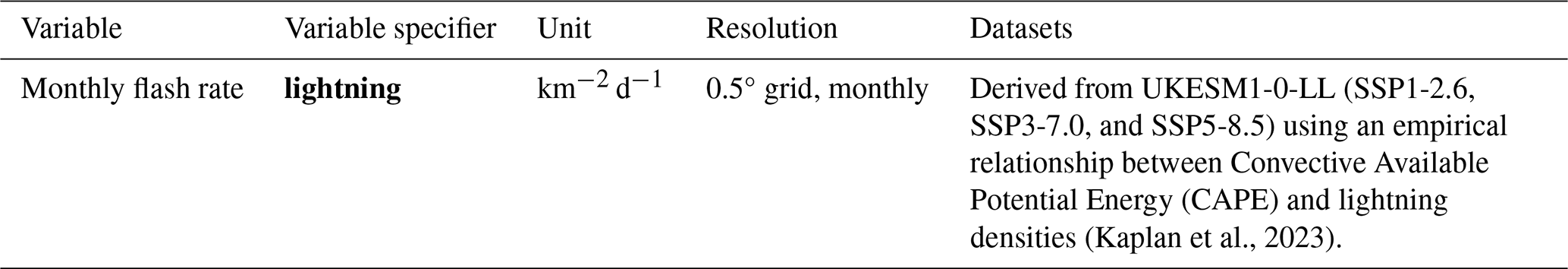
This paper gives an overview over the ISIMIP3b, group I and II experiments and the provided climate-related forcing data sets. The simulations assuming fixed 2015 direct human forcings and a low (ssp126) and two high emission scenarios (ssp370 and ssp585) are designed to describe the impacts of different levels of climate change on present day natural and human systems.

This paper is intended to work as a catalogue where the climate impact modellers can find all relevant information (data source, formats, resolution, covered time period etc.) about the climate-related forcings selected as input for the impact model simulations generated within the CMIP6-based ISIMIP3b, group I (historical period) and group II (future projections) framework. As a continuous process we would like to improve or complement these data sets wherever possible. So this paper can also be read as a call to either contribute by additional input data that allows other sectors to join the current simulation round or by methods that could be used to generate additional data sets for the next simulation round that will likely build on CMIP7 simulations. The following climate-related forcings have been identified as still missing and particularly critical to be added to a fourth simulation round of ISIMIP: (i) temporally resolved lightning data accounting for changes in climate, (ii) bias-adjusted oceanic forcing data, (iii) projected coastal water levels in high temporal resolution accounting for extremes and representing the effects of long term sea level rise in line with the underlying global climate simulations, and (iv) ozone concentration fields in line with the GCM simulations. While a bias-adjustment of the oceanic forcings is already suggested in Sect. 3.4.2, the approach does not preserve the daily variability of the raw oceanic forcings as it requires atmospheric surface flux only available in monthly resolution from the ISIMIP3b GCMs. To ensure the consistency on daily time scale, we have submitted an associated request for CMIP7 whose simulations will be used within the next round of ISIMIP. The generation of high resolution coastal water levels is ongoing research described in Sect. 3.2.3. In particular the generation of the short term variability that will have to be added to the long term trends in water levels still has to be developed and prove to fulfill the demands. In addition, it would be great to also provide estimates of the extreme coastal water levels associated with the tropical cyclone tracks and wind fields we provide within ISIMIP3b (see Sect. 3.2). There is a general demand for higher resolution CRF including both, the oceanic and the atmospheric components ideally accounting for heat island effects. As the ISIMIP CRF have to be globally consistent in the sense that they have to represent the daily variability of the underlying coarse resolution GCMs, we cannot use data from dynamical downscaling approaches using boundary conditions from different GCM runs as for example available through CORDEX. However, it seems to be appealing to harmonize the selection of the ISIMIP GCMs with a priority setting regarding the GCM-based boundary conditions within CORDEX.

The climate-related forcings described here are also provided as input for the new ISIMIP3b, group III simulations where the associated Direct Human Forcings (DHF) are not held constant at 2015 levels but are projected into the future in line with (i) the population growth and economic development associated with the considered Shared Socioeconomic Pathways (SSPs) and mitigation measures required to reach the prescribed levels of climate forcings associated with the climate projections (“no adaptation” experiments) and (ii) additionally accounting for the impacts of climate change (“adaptation” experiments). The collection of the associated DHF will be described in a separate paper.