PALM-meteo 2.8: Processor of PALM meteorological input data

PALM is a versatile and modular microscale atmospheric modelling system. It supports offline nesting using pre-processed initial and boundary conditions provided via the dynamic driver file, along with other time-dependent input data, such as radiative forcing. PALM-meteo is a new modular tool for preparing PALM dynamic drivers using data from various mesoscale or global meteorological models as well as other sources, such as measurements. It is derived from an older tool, the WRF_interface, which provided dynamic drivers using WRF (Weather Research and Forecasting) model data. PALM-meteo significantly expands the scope of usable meteorological and chemical inputs for PALM (currently supporting WRF, ICON, Aladin, CAMx, and CAMS) and is readily extendable to additional data sources in the future. Its processing capabilities extend beyond simple conversion and interpolation, including vertical adaptation, mass balancing, wind damping, and other features. The applicability of this versatile tool has been demonstrated by several studies, including the validation of PALM model simulations and various scenario simulations, e.g., in Prague (Czech Republic), Bergen (Norway), Guelph (Canada), Milan and Bologna (Italy), Berlin and Leipzig (Germany), or Vienna (Austria).

1 Introduction

Recent research progress in numerical weather and climate simulations of urbanised areas has developed to include higher spatial and temporal resolutions (Hamdi et al., 2020). Feedback from microscale processes impacted by surface heterogeneities can be explicitly resolved and better represented, enabling detailed assessments of urban atmosphere dynamics and further supporting adaptation of cities to climate change and mitigation of its impacts (González et al., 2021; Masson et al., 2020; Yang et al., 2023).

The increased sophistication of microscale meteorological tools stresses the fidelity and realism of their input data, i.e., land use, building morphology, turbulence, meteorological inflow conditions, etc. (Belda et al., 2021; Dauxois et al., 2021; Radović et al., 2024). Among the components mentioned, constraining microscale simulations across the simulation domain with properly derived meteorological input data is a decisive factor that affects the flow development within the high-resolution domain (Ehrhard et al., 2000; Xie and Castro, 2008; Talbot et al., 2012; Wyszogrodzki et al., 2012).

Widely used numerical weather prediction (NWP) models simulate regional atmospheric flows in real meteorological conditions, but their spatial and vertical resolution usually does not reach the meter-scale resolution necessary to capture individual components of the urban landscape (e.g., streets or buildings). On the other hand, microscale modelling tools – though powerful for assessing street-scale urban microclimate processes – do not contain information about the primary drivers of day-to-day weather variations, i.e., synoptic-scale systems (Maronga et al., 2015; Baklanov et al., 2018). As a result, an integral aspect of urban micro-meteorological modelling involves developing methods for utilising and generating initial and boundary conditions (IBC) from larger-scale (mesoscale) models to drive microscale meteorological models (Maronga et al., 2020; Kadasch et al., 2021; Resler et al., 2021, 2024). The initial state of the atmosphere (i.e., initial conditions) at the beginning of the simulation, and the atmospheric conditions imposed at the edges of the computational domain (i.e., boundary conditions), control and determine the flow evolution during the simulation period in limited-area models. Hence, to ensure realistic and physically consistent simulations of urban airflow, microscale models must be adequately connected to the real atmosphere through the IBC. Nonetheless, transforming mesoscale data from synoptic to city- and street-scales is a non-trivial, technically complex task and requires well-developed and specialised tools capable of bridging the gap between meso- and microscale model differences (e.g., scale gap, temporal resolution, grid incompatibility, physical inconsistencies; Wiersema et al., 2020).

1.1 Initial and boundary condition methods

To date, various types of IBC have been used to constrain microscale simulations at the lateral, top, and bottom sides of the simulation domain. Depending on the experimental design and objectives, the strategies for providing IBC, along with their corresponding mathematical formulations, vary. The most common and straightforward methods include idealised forcings, such as Dirichlet or Neumann conditions, which prescribe fixed physical values and constant gradients, respectively. In studies that consider idealised domain geometry, cyclic (periodic) boundary conditions can be employed. In other cases, observation-based forcing data (e.g., radiosonde vertical profiles) can be utilised. Still, due to their spatiotemporal scarcity, lack of consistency across a simulation domain, and limited representation of the real state of the atmosphere, they present a suboptimal choice for microscale model forcing.

Along with the methods for implementing boundary constraints, boundary input data categories must be defined. As a baseline, thermodynamic (i.e., temperature) and dynamic (i.e., wind velocity) boundary conditions must be provided. Furthermore, urban-scale simulations require consistent radiative forcing, which is essential to accurately capture energy transfer and surface-atmosphere radiation interactions, which are key drivers in the atmospheric boundary layer. It is typically provided through short- and longwave downwelling fluxes at the top of the domain and can be derived from the mesoscale models or observations. Finally, depending on the modelling goals (e.g., in air quality modelling simulations), inputs containing chemical species specifications are also required. These are typically derived from observation stations or chemical transport models and include background concentrations of chemical species such as nitrogen oxides, carbon monoxide, ozone, and particulate matter.

For the real-case microscale simulations, coupling microscale with mesoscale models is vital (Kadaverugu et al., 2019; Wong et al., 2021; San Jose and Perez-Camanyo, 2022). Microscale-mesoscale model coupling strategies for exchanging data broadly encompass two categories, i.e., online and offline (Baklanov et al., 2014; Kadasch et al., 2021). The former implies simultaneous model execution and data exchange (possibly including feedback from the microscale into the mesoscale model), while the latter refers to running the mesoscale model first, storing its output, and feeding information to the microscale model through boundary conditions, continuously updating them over time throughout the simulation. The adopted coupling strategy depends on various factors, such as application purposes, computational resources, etc. Nevertheless, even though the online coupling offers more realistic assessments, the offline one is routinely employed in the PALM model's framework and offers greater flexibility while providing sufficiently accurate results.

1.2 The PALM model system

The PALM model system (Maronga et al., 2020) is an open-source, complex microscale meteorological model. It is usually utilised with the LES core that solves non-hydrostatic, filtered, Boussinesq-approximated, incompressible Navier-Stokes equations, however the RANS core is also implemented. The model is equipped with multiple components enabling realistic simulations of urban environments, in particular the land surface model (LSM; Gehrke et al., 2021), building surface model (BSM; Resler et al., 2017; Maronga et al., 2020), radiative transfer model and plant canopy model (RTM and PCM; Krč et al., 2021), single-layer urban canopy model (SLURB; Karttunen et al., 2025), human biometeorology module (BIO; Fröhlich and Matzarakis, 2020), chemistry model (CHEM; Khan et al., 2021), online nesting (Hellsten et al., 2021) and mesoscale nesting (MESO; Kadasch et al., 2021). The model and its individual components have been validated multiple times against tunnel measurements (e.g., Gronemeier et al., 2021; Řezníček et al., 2023) and in real environments (e.g., Resler et al., 2017, 2021, 2024). The model has been used for research as well as for urbanistic studies in different parts of the world. The input data needed for complex simulation setups can be provided in specific NetCDF files called drivers according to the PALM Input Data Standard. These drivers provide, e.g., domain configuration including terrain, soil, trees, and buildings (Static driver), initial and boundary meteorological and air quality conditions (Dynamic driver), unresolved urban layer description (SLURB driver), emissions (Chemistry driver), and traffic-related information (Traffic driver).

1.3 IBC and the dynamic driver in PALM

PALM contains various options for setting IBC. Separate boundary condition types can be set for the left-right, north-south, bottom, and top boundaries. They can be set for all quantities or specified separately for different quantities, e.g., pressure, potential temperature, or subgrid-scale turbulence kinetic energy (TKE). The condition can be set to Dirichlet, Neumann, or cyclic. The initial conditions can be set in various ways; the most common are setting constant profiles or by solving the 1-D model for the vertical profile of the quantity. The IBCs can be complemented by a large-scale forcing and nudging mechanism to drag vertical profiles to prescribed values. All these options are intended mainly for use in synthetic idealised experiments, which are not meant to represent actual atmospheric conditions at a specific point in time and space. In real or realistic experiments, PALM implements a mechanism called offline nesting. This setting dynamically sets the boundary conditions to Dirichlet on the inflow and Radiation on the outflow parts of the lateral and top boundaries.

Supplying IBC for PALM simulations is managed through the so-called dynamic driver input file (named PIDS_DYNAMIC in PALM's working directory). The mentioned file comprises time-dependent meteorological data, large-scale forcing tendencies, radiation fields, and, optionally, chemical species data. It is utilised from the beginning of the simulation, providing the initial conditions for the entire domain and time-dependent lateral and top boundary conditions for the duration of the simulation. The core variables provided are the 3-D fields of potential temperature (θ), velocity components (u, v, w), and water vapour mixing ratio (q_v). In addition, the 3-D fields of soil moisture and temperature, as well as a 1-D time series of large-scale surface forcing of surface pressure, are included as additional mesoscale-derived bottom boundary constraints. Radiation-associated variables, such as short- and longwave downwelling radiation and shortwave downwelling diffuse radiation, are provided for cases that utilise external radiative forcing. In setups involving chemistry modelling, the IBC of the concentrations of the configured chemical species are provided as well, although until recently, the initial conditions could be only provided as vertical profiles (lod=1; see Sect. 2.2.2). Lateral boundary conditions are provided only at the outermost grid row/column of the PALM domain (i.e., no relaxation of the BC in a buffer zone is performed).

When applying the boundary conditions from the dynamic driver, PALM internally performs linear interpolation in time, so that the variables may be provided at their original temporal resolution, thus reducing the size of the dynamic driver. Moreover, PALM dynamically adjusts its timestep length, so the actual PALM timesteps are not known in advance. All the listed variables have a common time dimension called time, except for the radiation variables, which have their own time dimension called time_rad. It is very common to have mesoscale model outputs in 1 h intervals, which may be insufficient for radiation (especially shortwave), hence the possibility of providing it at a finer temporal resolution.

1.4 Existing tools for PALM dynamic drivers

Considering that mesoscale data processing and further coupling to the high-resolution microscale domain are not a part of PALM's internal structure, this process has to be executed as a preprocessing step before PALM's utilisation. Multiple preprocessors exist to facilitate the dynamical downscaling process and create PALM-consistent input, e.g., WRF_interface (WRF_interface, 2020), WRF4PALM (Lin et al., 2021), or SanDyPALM (Vogel et al., 2025) for the WRF (Weather Research and Forecasting) model outputs or INIFOR (Kadasch et al., 2021) for the COSMO model outputs. Achieving a user-oriented, streamlined coupling interface characterised by flexibility of coupling to multiple mesoscale and chemical models and transparency in a standardised workflow is a technically complex and laborious task. Most importantly, ensuring physical realism and internal consistency between the two models during the downscaling process across coupled domains requires a robust coupling framework. To address these challenges, we present PALM-meteo 2.8, a processor designed to convert, reformat, and adjust meteorological, radiation fields, and chemical species to drive PALM simulations, bridging the interface between a variety of mesoscale weather and chemistry models and high-resolution microscale model.

1.5 Previous studies using PALM-meteo and its predecessors

The first version of the PALM-meteo was created in the winter of 2020 together with Deutscher Wetterdienst (DWD) project PAMORE, as a more advanced and modular replacement for the older tool WRF_interface (WRF_interface, 2020). However, the projects split, and the current PALM-meteo version contains no DWD-developed code or methods. The older tool was used in several studies in Prague (Czech Republic) (Belda et al., 2021; Geletič et al., 2021; Resler et al., 2021) and in Vienna (Austria) (Žuvela-Aloise et al., 2025).

Previous versions of the PALM-meteo were used for PALM dynamic driver preprocessing in several studies in various cities. Examples of the papers utilising results from the PALM-meteo are mainly from Prague (Geletič et al., 2022, 2023; Janků et al., 2024; Patiño et al., 2024; Radović et al., 2024; Resler et al., 2024; Řezníček et al., 2025), Bergen (Norway) (Esau et al., 2024), or Guelph (Ontario, Canada) (Wang et al., 2025). Moreover, a study by Resler et al. (2024) uses IBC created by PALM-meteo from various regional climate models, including WRF, ICON, and Aladin.

A methodical approach presented in Radović et al. (2024) evaluated the PALM model system's performance and sensitivity across a series of different WRF model-derived boundary inputs under distinct meteorological scenarios. The authors demonstrated the microscale model's ability to attenuate the transferred driving data biases and stressed the importance of accuracy and careful selection of the mesoscale forcing. More precisely, the study presents the challenges of obtaining accurate boundary conditions for the microscale PALM model by utilising an ensemble of 16 WRF configurations across four seasons. The results showed that PALM is inherently dependent on the quality of its mesoscale boundary conditions. Radović et al. (2024) is focused primarily on wind speed in 10 m and air temperature in 2 m, as a typically measured meteorological variables. PALM's high-resolution simulations can partially attenuate errors in wind speed but cannot entirely correct errors in air temperature. Since the experiment established that the mesoscale model is a primary source of bias, the study stresses the need for rigorous evaluation and meticulous construction and selection of boundary conditions to achieve reliable PALM simulations. Currently, there is no published sensitivity study focused on shortwave and longwave radiation, as well as the effect of various urban parameterisations.

Thanks to a relatively stable specification of PALM's dynamic driver, there is a high cross-compatibility between dynamic drivers created in PALM-meteo and various PALM versions. In general, new PALM-meteo versions are tested with new PALM versions, and since version 24.04, the PALM model system releases are bundled with up-to-date PALM-meteo versions. However, there is no need to select specific versions of either programs for the purpose of mutual compatibility. During PALM-meteo development, there were only a small number of changes that could cause incompatibility of dynamic drivers from older versions of PALM-meteo when used in newer PALM versions, such as the addition of a compulsory LOD attribute for variables (see also Sect. 2.2.2) or a change in the verification of the z-coordinate variable. Therefore, it is recommended to always use the latest version of PALM-meteo.

2 Description of PALM-meteo

The main goal of PALM-meteo is to convert coarse-resolution atmospheric data onto the PALM model grid (see illustration in Fig. 1) and process them into the PALM dynamic driver with IBC and other desired meteorological inputs.

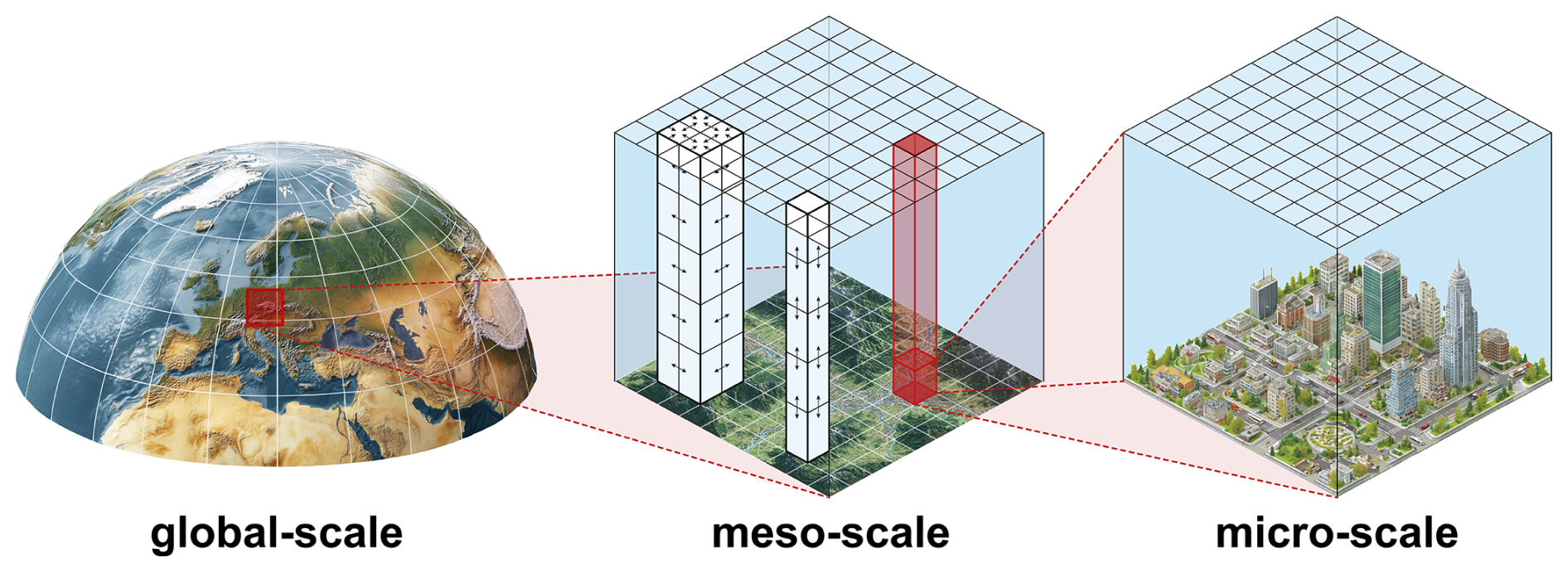
Figure 1 Illustration of the downscaling via horizontal and vertical interpolation in a typical PALM toolchain with PALM-meteo. The first step is performed within mesoscale model by transferring data from a global scale model. The second step is carried out in PALM-meteo, where horizontal and vertical interpolation or adaptation are required (illustrated by the white columns and arrows in the second panel). After this processing, part of the red column(s) is prescribed as boundary conditions for the microscale model.

PALM-meteo can take input data from a variety of sources, but the most common scenario is using 3-D outputs from a mesoscale atmospheric model, either from a forecast or from a (re)analysis. In this approach, the subsequent PALM simulation can be viewed as downscaling of the mesoscale model data, although in some cases PALM's static input data (such as buildings or vegetation) may represent a scenario which differs from the reality represented in the mesoscale model.

In the typical mesoscale nesting scenario, there is a very large gap in horizontal resolutions (typically units of kilometres versus units of metres). This is one of the reasons why such microscale simulations usually apply a temporal spin-up after the initial state, as well as a rather large spatial buffer at the windward side (typically several hundred metres or several kilometres for moderate wind speeds), such that PALM can develop realistic flow with appropriate resolved and subgrid-scale turbulence. To save computational resources, this is in most cases accomplished by having a larger parent domain with coarser resolution into which the fine-scale domain for the area of interest is nested; the nesting may also be multi-level. The Synthetic Turbulence Generator in PALM generates turbulence at the inflow boundary, but it does not alleviate the need for a sufficient buffer area. Having this in mind, PALM-meteo does not perform any specific surface diagnostics beyond the state provided by the input data. In the vertical dimension, where the gap in resolutions is typically much smaller, it uses only interpolation and extrapolation of the input levels; any further refinement is left to the inflow area of the PALM simulation.

2.1 PALM-meteo architecture

The generation of a dynamic driver proceeds in six stages:

1. check_config: validation of user configuration

2. setup_model: set-up of simulation domain projection, geometry, and properties

3. import_data: loading of data from input files (such as mesoscale model outputs), including initial data conversions

4. hinterp: horizontal interpolation, usually in the form of regridding

5. vinterp: vertical adaptation and interpolation

6. write: generation of a finalised PALM dynamic driver, post-processing.

This order of operations is fixed due to multiple interdependencies. Specifically, performing vertical interpolation after horizontal is required for vertical adaptation to the fine-resolution terrain, see Sect. 2.2.3.

Due to potentially large amounts of data processed by PALM-meteo, most of the intermediate data is passed from one stage to the next via an intermediate file. This program design has several key advantages. Because each stage can be executed in its entirety, it is possible to stop the process between two stages and continue it later, possibly on a different machine. If a change is induced that affects only some later stages, it is not necessary to re-run the preceding stages. It is also possible to examine the well-defined intermediate results, which, in combination with executing individual stages, greatly help with debugging and parameter tuning. The partially or wholly interpolated values may also be useful in scientific analyses regarding the PALM simulation for which they are prepared.

This design approach was chosen over an alternative design in which the program would process data in smaller chunks that always fit into memory (such as the values for a single variable and a single time step), continuously from the beginning until they are written to the dynamic driver. Such a design could avoid the intermediate files, thus saving some time and storage space. However, it would also need to reinitialise the processing of each stage for each chunk of data, and it could lead to further complications in cases where there are interactions and dependencies between individual variables (e.g., when they are related to the same physical quantity) or time-steps (e.g., with temporal (dis-)aggregation).

More details about the architecture and implementation of PALM-meteo are available in the Appendix A

2.2 Common capabilities

PALM assumes that the IBC are hydrostatic; therefore, it takes pressure only as a time series of values that represent the common hydrostatic pressure at the base model level (origin_z). For the current input modules that import data from non-hydrostatic models (WRF, ICON, Aladin), the base level pressure is taken from the surface pressure and adjusted using the barometric formula, which assumes the dry adiabatic lapse rate of $\frac{g}{c_p}$:

$$\begin{array}{}\text{(1)}& P_{\mathrm{b}}=P_{\mathrm{s}}{\left(\mathrm{1}-{\displaystyle \frac{(h_{\mathrm{b}}-h_{\mathrm{s}})g}{c_p{T}_{\mathrm{s}}}}\right)}^{\frac{c_p}{R_{\mathrm{d}}}}\end{array}$$

where P_s is the input model's surface pressure, T_s is air temperature at surface, h_s is the surface elevation, h_b is the PALM base level elevation, c_p is the isobaric heat capacity of air, R_d is the specific gas constant of (dry) air and g is the acceleration of gravity.

The base-level pressure is calculated from Eq. (1) for each PALM model column and then averaged spatially. The resulting common base level pressure is written in the dynamic driver variable surface_forcing_surface_pressure (which actually specifies base level pressure, not surface pressure as the name suggests), and it is also used in other PALM-meteo calculations that deal with hydrostatic pressure.

2.2.1 Forecast cycles

For most PALM-meteo plugins, the input data comes from either a forecast model or a (re)analysis. In either case, the input data may come from one or more forecast/data assimilation cycles. In the case of a forecast, the data are labelled by their cycle (typically the time of their last analysis) and the time of validity; the forecast horizon is the distance between the cycle and the validity time. For analyses divided into cycles spanning multiple times of validity, we use an equally defined horizon as a purely technical label.

The user's data archive may contain overlapping forecast/assimilation cycles (i.e., where the horizons are longer than the interval between the cycles). In that case, PALM-meteo allows a versatile selection of input data such that they form a continuous (equidistant) time series. Typical global or mesoscale numerical weather models use either four or eight cycles every day, starting at midnight UTC; the user may select all or a subset of cycles by specifying a regular cycle interval. In addition to that, the earliest usable horizon may be specified in case the early horizons should be disregarded as a model spin-up or stabilisation period.

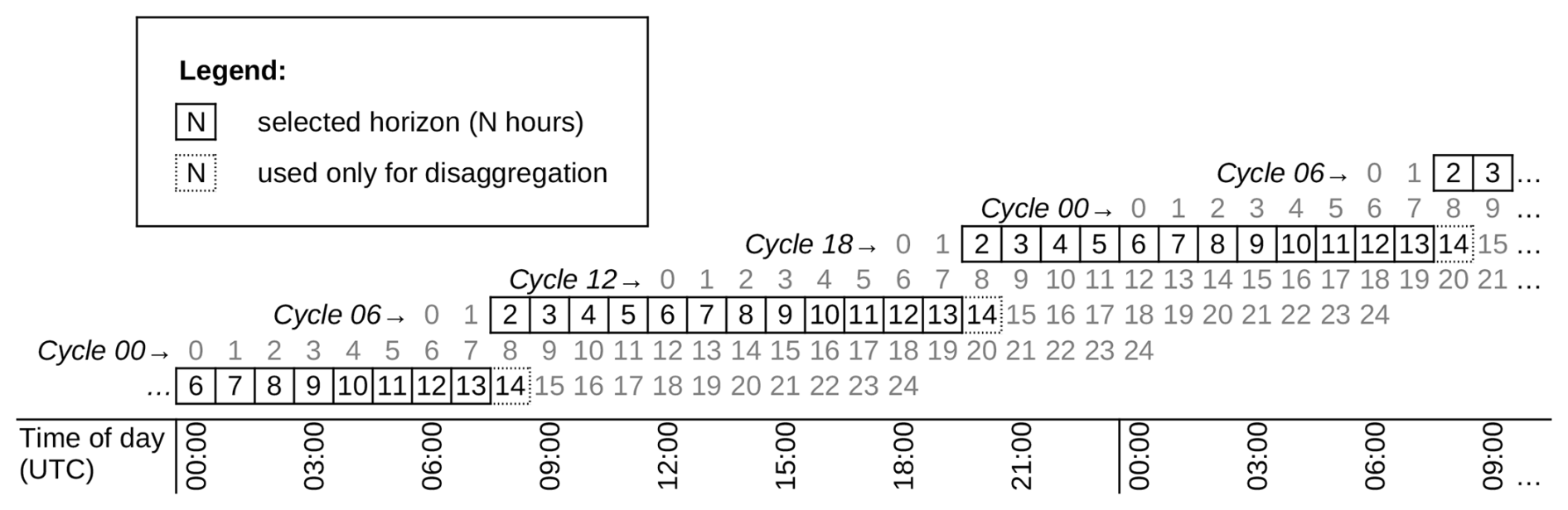
Figure 2 Example of forecast cycle and horizon selection. The user database contains hourly data from forecast cycles at 00:00, 06:00, 12:00 and 18:00 UTC; each forecast contains 25 h of data (00:00–24:00 UTC). The user selects 06:00 UTC as the reference cycle, 12 h as the cycle interval (thereby skipping cycles 00:00 and 12:00 UTC) and 2 h as the earliest horizon. The times 08:00–19:00 UTC are taken from the forecast cycle at 06:00 UTC of that day, and the times 20:00–07:00 UTC are taken from the forecast cycle at 18:00 UTC. In addition, the data from 20:00 UTC from the cycle 06:00 UTC and 08:00 UTC from the cycle 18:00 UTC are used as the right-hand side of the temporal disaggregation interval.

If the input data contains temporal averages or accumulations that need to be temporally disaggregated for the use in PALM, the disaggregation is only valid between subsequent timesteps of the same cycle. In that case, one further (overlapping) horizon needs to be selected from each cycle to be used as the right-hand side of the disaggregation interval. See Fig. 2 as an example. Additionally, since the disaggregated values represent the centres of the intervals between timesteps, it is possible to either use one extra timestep before and after the simulation period for the disaggregated values, or to extrapolate these ends if the respective input files are not available.

Combining data from multiple forecast cycles is favourable for longer simulations, as it uses earlier forecast horizons that have lower forecast errors than later horizons. On the other hand, it may lead to unnatural jumps in the data at the seams between the cycles. For that reason, it may be preferred to use a single forecast cycle for shorter simulations if the available forecast horizons cover the full duration of the PALM simulation. The configuration allows to select a single cycle as an alternative to the cycle interval.

As a third option, the user may choose to ignore the forecast/assimilation cycle information and use all provided input files, assuming they already form a continuous time series.

2.2.2 LOD=1 conversion

By default, the initial conditions are provided as a full 3-D field, specified in the dynamic driver by assigning the value 2 to the lod (level of detail) attribute. PALM also supports 1-D vertical profiles, which are specified as lod=1. The 1-D profiles may be used for debugging PALM, or if lod=2 leads to unexpected errors. PALM-meteo supports creating these profiles as horizontal averages over the model domain using the pt (potential temperature), qv (humidity), and uvw (wind field) options in the output:lod configuration section.

2.2.3 Vertical adaptation method

An important issue when preparing all 3-D fields for IBC is the matching of vertical coordinates. Because the resolution of the PALM model and the resolution of input data (e.g., from a mesoscale model) differ greatly (typically by 3+ orders of magnitude), the representation of terrain height differs as well. Apart from different resolutions, other reasons for the difference in terrain height are different data sources and/or processing methods. Therefore, PALM-meteo needs to match vertical coordinates with a potentially different terrain height. This is done as part of vertical interpolation. In general, there are three possible solutions to match vertical coordinates:

1. Maintain level height (either as hydrostatic pressure or as height above mean sea level – a.m.s.l.), disregarding differences in terrain. This leads to major problems: when the target (PALM) terrain at a specific horizontal point is lower than the terrain in the input data, the values between the two terrain heights need to be extrapolated; in the opposite case, the data between the two terrains are discarded. Any surface-related effects, such as wind drag or strong vertical gradients in temperature and humidity, will be positioned improperly.

2. Shift data vertically so that terrain height is matched. In other words, maintain the above-ground level (AGL) height in the input data. With this approach, the surface-related effects will be preserved correctly, but the vertical shift will remain constant for all levels. If the vertical gradients in the upper levels for the respective variables are not negligible and the terrain has steep slopes leading to uneven vertical shifts, this translates to strong horizontal gradients in the upper levels of the resulting 3-D field. This can lead to problems in the PALM model, such as the formation of unrealistic gravity waves.

3. Match the terrain at the lower levels, keep zero or small vertical shifts in the upper levels and stretch or squeeze the levels in between. This approach is used in PALM-meteo under the name vertical adaptation.

The vertical adaptation method in PALM-meteo was initially inspired by the hybrid vertical levels in the WRF model. WRF uses either the sigma levels, where each level is defined by a constant ratio between the model top pressure and the surface hydrostatic pressure at each grid point, or the hybrid levels, which are isobaric above a certain level and gradually transition to terrain-following below that level. For the WRF model, PALM-meteo allows the user to use an analogous method for the vertical adaptation (such as if the terrain in WRF was changed internally to match the PALM terrain). By selecting the adequate choice sigma or hybrid for the configuration option wrf:vertical_adaptation, depending on the WRF setup, PALM-meteo loads the corresponding level metadata from the WRFOUT files and shifts the levels accordingly as part of the vinterp stage.

However, these two methods are only applicable to WRF data. In addition to that, both the sigma and hybrid methods typically leave too strong horizontal gradients for PALM configurations with resolutions in the order of metres and with coarse terrain. To counter that, a third method called universal has been implemented. This method uses user-specified transition level (configured as vinterp:transition_level)

In the next step, the vertical interpolation of the 3-D fields together with terrain matching and vertical adaptation is performed for each PALM grid column linearly on the pressure coordinates, where the shifted pressure ${\stackrel{\mathrm{̃}}{p}}_{l_n}^{\mathrm{W}}$ of WRF level n is calculated as

$$\begin{array}{}\text{(2)}& {\stackrel{\mathrm{̃}}{p}}_{l_n}^{\mathrm{W}}=\left\{\begin{array}{ll}\left(p_{l_n}^{\mathrm{W}}-p_{\mathrm{t}}\right)\frac{p_{\mathrm{s}}^{\mathrm{P}}-p_{\mathrm{t}}}{p_{\mathrm{s}}^{\mathrm{W}}-p_{\mathrm{t}}}+p_{\mathrm{t}},& \text{if }{p}_{l_n}^{\mathrm{W}}>p_{\mathrm{t}}\\ p_{l_n}^{\mathrm{W}},& \text{if }{p}_{l_n}^{\mathrm{W}}\le p_{\mathrm{t}}\end{array}\right.\end{array}$$

where $p_{l_n}^{\mathrm{W}}$ is the original WRF level n pressure, $p_{\mathrm{s}}^{\mathrm{W}}$ is the WRF surface pressure, $p_{\mathrm{s}}^{\mathrm{P}}$ is the pressure corresponding to the PALM terrain and p_t is the transition level pressure (the upper stretching limit), which is taken from the average pressure at the configured height above the highest obstacles (terrain, buildings or plant canopy) in the domain. The corresponding option transition_level has a default value of 300 m, but if the user can assess the height at which the effect of surface friction is no longer apparent in the context of relevant weather and surface roughness, it is recommended to specify this. An example of the universal vertical adaptation method is presented in Fig. 3. In this setup for Prague, the transition level was set to 2179 m a.m.s.l., so the WRF layers above that are unchanged and the layers below shift progressively to match the more detailed terrain.

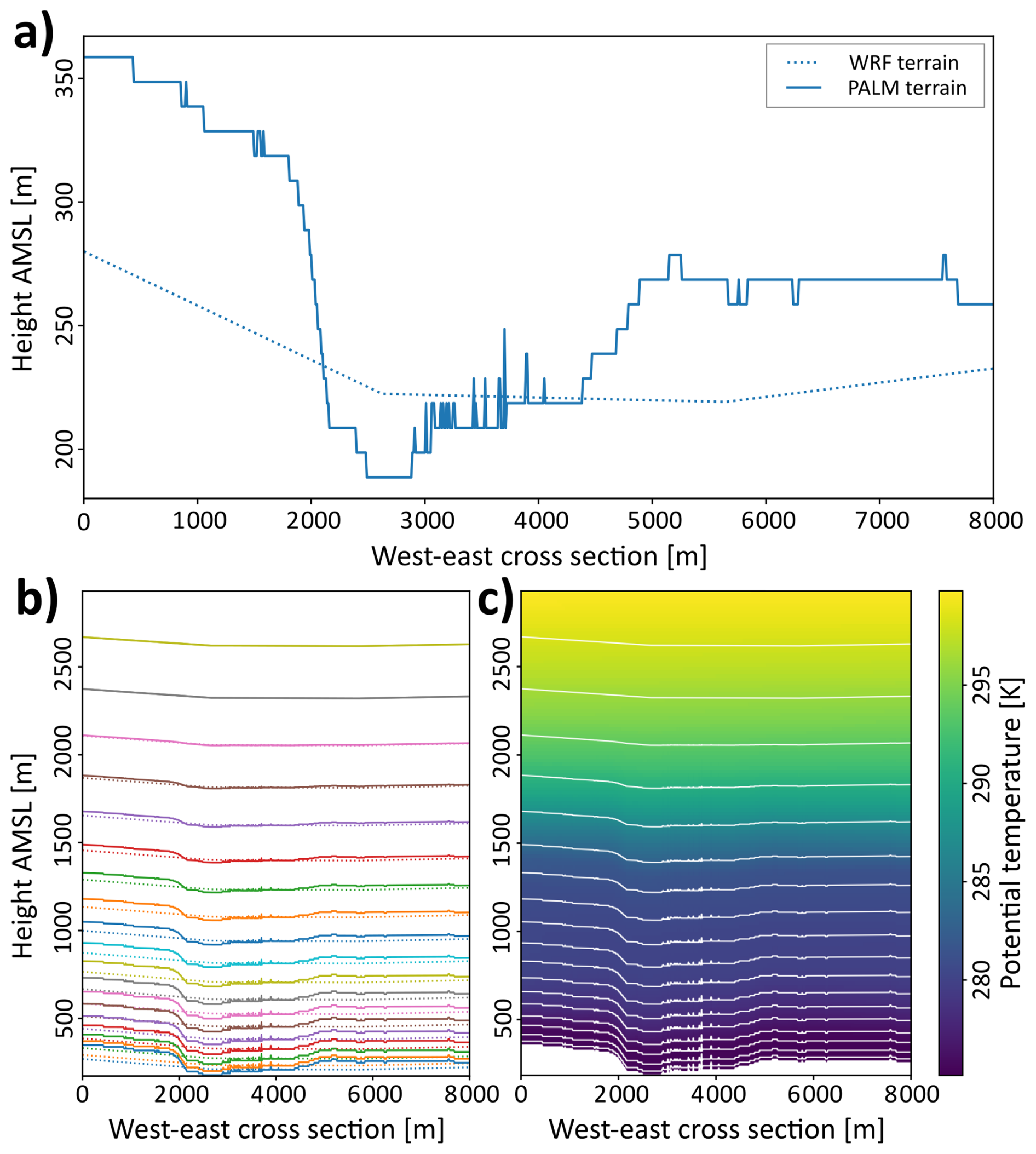
Figure 3 Illustration of the vertical adaptation method: Example scenario of the Vltava river valley in Prague, west–east cross sections with elevations exaggerated. (a) Mismatch of the interpolated coarse terrain from the 3 km WRF model and the fine terrain of the PALM model. (b) Structure of the individual vertical layers of the WRF model (dashed lines) and the position to which they are shifted by the vertical adaptation method (full lines of the same colour). (c) Final vertically interpolated 3-D field (potential temperature) with the overlay of the shifted WRF levels from which the interpolation is performed.

2.2.4 Vertical interpolation

For large simulations, the vertical interpolation is typically the longest stage of PALM-meteo processing due to the simple fact that it processes the largest amount of data (full 3-D fields on the fine PALM grid). PALM-meteo currently offers three different implementations of the actual vertical interpolation routine, and the user may select the preferred implementation using the configuration option vinterp:interpolator.

The metpy interpolator is the legacy option which uses the interpolate_1d function from the MetPy (NSF Unidata, 2025) library, which is an optional dependency. In most cases, this is the slowest implementation.

The prepared interpolator is the default option. It is fully implemented in Python (NumPy) within PALM-meteo, and it works in two stages: first, it calculates and stores the interpolation weights based on source and target vertical coordinates, and then it uses these weights to perform the linear interpolation, which is done repeatedly for all fields to which those vertical coordinates apply. This interpolator is typically much faster than metpy.

The fortran interpolator uses a Fortran routine that needs to be compiled into native code using the f2py tool, which is shipped with NumPy (a dependency of PALM-meteo). This interpolator is by far the fastest of the three and should be preferred for large scenarios, if possible.

For vertical interpolation of the wind components u, v, and w, the vertical interpolation is linear by default, which should be sufficient for most scenarios. It is also possible to interpolate between the source model levels using the wind profile power law. This law is normally used for estimating horizontal wind speed at height z from the wind speed u_r at the reference height above ground z_r using the formula

$$\begin{array}{}\text{(3)}& u=u_{\mathrm{r}}{\left({\displaystyle \frac{z}{z_{\mathrm{r}}}}\right)}^{\mathit{\alpha }}.\end{array}$$

This method may be generalised for interpolation at height z_m between levels z_b and z_t with wind speeds u_b and u_t respectively:

$$\begin{array}{}\text{(4)}& u_{\mathrm{m}}=u_{\mathrm{b}}+\left(u_{\mathrm{t}}-u_{\mathrm{b}}\right){\displaystyle \frac{z_{\mathrm{m}}^{\mathit{\alpha }}-z_{\mathrm{b}}^{\mathit{\alpha }}}{z_{\mathrm{t}}^{\mathit{\alpha }}-z_{\mathrm{b}}^{\mathit{\alpha }}}}\end{array}$$

which is equivalent to the original formula (3) in the case where the bottom level is the ground ($u_{\mathrm{b}}=z_{\mathrm{b}}=\mathrm{0}$).

This method is intended for special cases, such as fine-resolution small-scale scenarios where there are insufficient near-surface vertical levels in the input data. In that case, the user needs to estimate the appropriate value of α (e.g., α=0.143), set the configuration of vinterp:wind_power_law to that value and check the results for inconsistencies.

2.2.5 Mass balancing

When the dynamic driver is created, the cumulative inflow of air mass may not always equal the cumulative outflow for several reasons:

1. The input data (e.g., from the mesoscale model or manually prescribed profiles) need not be mass-balanced at the selected PALM boundaries, either due to the elasticity of the mesoscale model or due to the nature of the manually prescribed data.

2. The vertical adaptation method, if applied, does not guarantee that the balance between inflow and outflow is preserved perfectly.

3. A rounding error between the inflow and outflow may have been created with the spatial interpolation and resampling while creating the dynamic driver. For the non-linear air density profile, there is another potential source of discrepancy due to the linear interpolation.

4. When PALM applies the boundary conditions from the dynamic driver, another rounding error or non-linear discrepancy may be created due to temporal interpolation.

There are two available approximation systems for the flow equations in the PALM model. Both of them are incompressible; they do not consider the dynamic change of air density. The Boussinesq approximation, which is the default, assumes constant background air density across the whole simulated domain (only the influence mediated by potential temperature is considered). The other option, the anelastic approximation, assumes a fixed, horizontally constant air density profile.

PALM needs to ensure mass balance at all times. When offline nesting is enabled in PALM, this is performed at each timestep after applying the temporally interpolated boundary conditions by adding or subtracting the residual mass flux in the form of a constant vertical speed difference at the top boundary. This approach is simple, but limiting it to the top boundary means that the applied speed difference may be relatively high if the residual flux is high or if the aspect ratio of the domain is very high.

In order to remove most of the residual flux (points 1–3) in advance, PALM-meteo performs mass balancing by default as part of the last step when the dynamic driver file is written. Unlike the balancing method in PALM, this method distributes the residual flux evenly to all five borders. Thanks to the larger total border area, this method leads to smaller added speed differences.

The user needs to specify the planned approximation method for the PALM simulation using the configuration option simulation:approximation. For each of the five boundaries, PALM-meteo calculates the grid cell border area (taking into account the vertical stretching, if configured). At the lateral boundaries, PALM-meteo uses the terrain and building data provided by the static driver setup plugin (see Sect. 2.3.1) to identify the atmospheric (unblocked) border grid cells where the adjustment can be performed.

The residual mass flux (positive for inflow, negative for outflow) is calculated as

$$\begin{array}{}\text{(5)}& \mathrm{\Delta }{M}^{\mathrm{I}}=\sum _B\sum _{ij}{Q}_{B,i,j}^{\mathrm{I}}{\mathit{\rho }}_{i,j}\end{array}$$

with the volumetric inflows for the individual grid cell boundaries defined as

$$\begin{array}{}\text{(6)}& Q_{B,i,j}^{\mathrm{I}}=\left\{\begin{array}{ll}-V_{i,N^{\mathrm{Y}},j}{A}_{\mathrm{n},i,j}^B& \text{if }B=\mathrm{n}\text{ (north)}\\ V_{i,\mathrm{0},j}{A}_{\mathrm{s},ij}^B& \text{if }B=\mathrm{s}\text{ (south)}\\ -U_{N^X,i,j}{A}_{\mathrm{e},i,j}^B& \text{if }B=\mathrm{e}\text{ (east)}\\ U_{\mathrm{0},i,j}{A}_{\mathrm{w},ij}^B& \text{if }B=\mathrm{w}\text{ (west)}\\ -W_{i,j,N^Z}{A}_{\mathrm{t},i,j}^B& \text{if }B=\mathrm{t}\text{ (top)}\end{array}\right.,\end{array}$$

where $B\in \mathit{\{}\mathrm{n},\mathrm{s},\mathrm{e},\mathrm{w},\mathrm{t}\mathit{\}}$ identifies the respective lateral or top boundary, i and j index the individual grid cells adjacent to that boundary, and $A_{B,i,j}^B$ is the area of the boundary represented by that grid cell. $U_{i,j,k}$, $V_{i,j,k}$, and $W_{i,j,k}$ are the wind components, and the N^X, N^Y, and N^Z are the grid sizes in the respective dimensions. The air density ρ_i,j is used only in the case of the anelastic approximation.

Finally, the wind speed adjustment (positive for inflow), which is added to or subtracted from the corresponding boundary wind speed components as in Eq. (6), is calculated as $\frac{\mathrm{\Delta }{M}^{\mathrm{I}}}{A^B\mathit{\rho }}$ where $A^B={\sum }_B{\sum }_{i,j}{A}_{B,i,j}^B$ is the total area of all five boundaries.

PALM-meteo has the option of verifying the mass balancing by recalculating ΔM^I after its application; this prints a negligible non-zero value, which is the result of floating-point rounding errors.

2.2.6 Gas molar conversions

Upon loading the chemical input data, PALM-meteo performs automatic parsing and conversions of the decimal factors of the most commonly used units: ppmV, ppbV and µg m⁻³, g m⁻³, kg m⁻³.

However, this system is not well-suited for converting between molar fractions or volume concentrations (which PALM's chemistry module expects for gas-phase species) and mass concentrations (which PALM expects for non-gas-phase species, i.e., aerosols). The reason is that upon loading the chemistry input data, the precise air temperature and pressure are not yet known (they may already be loaded, but if they come from a separate meteorological model, they may be on a different grid).

This information is available on the PALM grid later in the last workflow stage, after the horizontal and vertical interpolation; therefore, the final unit conversion for chemistry is performed by the standard write plugin. Each time a quantity is marked as gas-phase (the attribute non_gasphase is false or missing) and it is provided as a mass concentration, its configured molar mass is used for conversion at the last stage.

Finally, in the very special case where the nitrogen oxide sum (NO_x) is requested to be calculated as a sum of nitric oxide (NO) and nitrogen dioxide (NO₂) and those quantities are provided as mass concentrations, they need to be converted to volume concentrations using their respective molar masses before the summation. In order to achieve that, there is a special option postproc:nox_post_sum which performs the summation of listed variables after their respective unit conversions.

2.3 Currently available modules

2.3.1 Set-up from static driver

This is currently the only way that PALM-meteo can perform the setup stage. This module loads a valid PALM static driver (by default taken from its standard PALM input file path) and sets up the following domain properties:

• horizontal domain structure (placement, geographic projection, and resolution),

• terrain, buildings, and plant canopy if present, also soil moisture adjustment, and

• simulation start time.

The vertical structure (size, resolution and optional grid stretching) and simulation length are not present in the static driver according to the PALM input data standard (PIDS), so they are taken from the configuration file. It is expected that an alternative to this module will be added in the future: a simple module which sets up the simulation purely from the configuration file for cases where the static driver is not (yet) available.

The specification of buildings in the PALM static driver provides several options, which makes it nontrivial to interpret the building data identically to how the PALM model does that. There are three main NetCDF variables which specify building data:

building_id

is an integer variable which, for each i,j coordinate, specifies the ID of the building on that point, thus separating the individual buildings horizontally.

buildings_2d

is a real-valued variable which is used to describe buildings in the 2.5-D geometry (without holes or overhangs). For each i,j coordinate, it specifies the building height in metres above terrain.

buildings_3d

is used to describe buildings with a full 3-D structure. It is a 3-D boolean variable which, for each $i,j,k$ point, specifies true if the respective grid cell lies within a building.

All buildings in the scenario are described as either 2.5-D or 3-D; if both variables are present, then only buildings_3d is used.

The vertical placement of the buildings is complicated by the fact that both variables specify the building shape with respect to the underlying terrain. The terrain is described as 2.5-D in the real-valued variable zt, which for each i,j specifies the terrain height in metres relative to origin_z, therefore PALM needs to discretise the terrain according to the vertical grid spacing dz. PALM-meteo, as well as any tool which needs to interpret terrain and/or buildings from the static driver, needs to perform identical discretisation to avoid mismatches. The same discretisation applies to the building heights in buildings_2d, while the heights of the terrain and the building are combined after the discretisation, not before. Finally, it is defined that if not all i,j points in the same building ID have identical terrain height, then the highest of such points determines the vertical placement of the respective building.

PALM-meteo carefully replicates the described building placement mechanism from the PALM model in order to identify buildings as obstacles for mass balancing (Sect. 2.2.5) and for the wind damping mechanism (Sect. 2.3.10). If there is a large number of individual buildings, this may slow down processing, as the horizontal grid mask needs to be processed for each building separately.

2.3.2 WRF

The WRF model is a state-of-the-art mesoscale numerical weather prediction system designed for both atmospheric research and operational forecasting applications. It features two dynamical cores, a data assimilation system, and a software architecture supporting parallel computation and system extensibility. The model serves a wide range of meteorological applications across scales from tens of meters to thousands of kilometres. The WRF development began in the latter 1990s as a collaborative partnership of the National Center for Atmospheric Research (NCAR), the National Oceanic and Atmospheric Administration (represented by the National Centers for Environmental Prediction (NCEP) and the Earth System Research Laboratory), the U.S. Air Force, the Naval Research Laboratory, the University of Oklahoma, and the Federal Aviation Administration (FAA). Nowadays, the WRF model is probably the most used model among scientists worldwide.

This was the first input module for PALM-meteo, created as a rewrite of the older WRF_interface tool, providing a full-featured replacement for the now-deprecated tool.

2.3.3 LCC projection in WRF

The recommended grid projection for using the WRF-ARW model in mid-latitudes is the Lambert conformal conic (LCC) projection. However, for the LCC projection, WRF does not use the standard WGS84 ellipsoid with a≈6378.1 km and b≈6356.8 km, but rather a computationally simpler sphere with r=6370 km (Snyder, 1987). In addition, when the WRF inputs are prepared using the built-in WRF Preprocessing System (WPS), any WGS-84 georeferenced input data are used directly as if they were referenced in the spherical coordinates, bypassing the conversion of geodetic latitude.

This approach is acceptable as long as the WRF outputs are treated in the same way – the XLAT and XLONG fields in the WRFOUT files do match the placement of the model grid. However, if somebody uses the LCC projection parameters from WRF to define the projection and then transforms the coordinates using a library that performs geodetic latitude conversion, such as the PROJ.4 library (PROJ, 2025), this leads to errors in latitude in the order of tens of kilometres. To avoid these errors, the conversion must not be done between the WRF LCC projection and the WGS84 (EPSG:4326) coordinates, but rather between the WRF LCC projection and the corresponding spherical coordinates. PALM-meteo uses this method to avoid the errors in latitudes. In addition, it allows to verify the projection parameters using the hinterp:validate option, available for all PALM-meteo input plugins.

2.3.4 WRF radiation

The WRF radiation plugin imports radiation data from the specified WRF output files. These may or may not be the same WRFOUT files used for atmospheric variables. If the main output file interval is 1 h, it is recommended to configure WRF to produce the AUXHIST files with radiation variables in a finer temporal resolution (e.g., 10 min).

There are multiple optional radiation modules in WRF, and some of these produce radiation outputs in different variables, so the variable names in PALM-meteo are configurable. The WRF files need to contain shortwave and longwave horizontal irradiance (marked in WRF as downward radiation) and, optionally, the diffuse component of the shortwave horizontal irradiance. If this component is not present, it is skipped from the dynamic driver, and the PALM radiation module uses its internal estimation of the direct/diffuse ratio.

2.3.5 ICON

The ICON (ICOsahedral Nonhydrostatic) modelling framework (Zängl et al., 2015) is a joint project of Deutscher Wetterdienst (DWD), Max-Planck-Institute for Meteorology (MPI-M), the German Climate Computing Center (DKRZ), the Karlsruhe Institute of Technology (KIT) and the Center for Climate Systems Modeling (C2SM) for developing a unified next-generation global numerical weather prediction and climate modelling system. ICON represents a flexible, scalable, high-performance modelling framework for weather, climate and environmental prediction. Its results provide actionable information for experts and wider society, and advance understanding of the Earth's climate system.

The ICON modelling framework offers a wide range of applications across all temporal and spatial scales. ICON can be used for global and regional numerical weather prediction as well as for global and regional climate simulations.

The ICON model utilises an icosahedral-triangular grid for its geographical projection rather than a traditional latitude-longitude grid. This grid is constructed by successively dividing the faces of an icosahedron, resulting in a mesh of triangular elements. The grid generation starts with an icosahedron inscribed in the sphere. Connecting the 12 vertices of the icosahedron with geodesic lines yields 20 equilateral spherical triangles with an edge length of about 7054 km. Iterative subdivision (e.g., bisection or trisection) of the triangle edges then yields a model grid with the desired spatial resolution. The effective mesh size of the model grid is defined as the square root of the mean area of the spherical triangles. In the current operational version, the global ICON grid has 2 949 120 triangles, corresponding to an average area of 173 km² and thus to an effective mesh size of about 13 km. All scalar prognostic model variables (e.g., temperature, density, moisture quantities) are located in the circumcenter of the triangles, whereas the edge-normal wind components are located in the edge midpoints.

The most important ICON prognostic variables are air density and virtual potential temperature (which allows diagnosing the pressure), horizontal and vertical wind speed, humidity, cloud water, cloud ice, rain, and snow. These variables are calculated for all grid cells at 90 terrain-following model levels extending from the surface to a height of 75 km, yielding a total of about 265 million grid points. Over land, additional prognostic equations are solved for soil temperature and soil water content for 7 soil levels.

PALM-meteo uses NetCDF files for the ICON input data. These can be provided directly by the PAMORE (PArallel MOdel data REtrieve from Oracle databases) (Deutscher Wetterdienst, 2025) service, or they can be obtained by converting the ICON GRIB files to NetCDF using Climate Data Operators (CDO; Max-Planck – Institut für Meteorologie, 2025).

For horizontal interpolation, PALM-meteo first performs Delaunay triangulation of the ICON grid points using the SciPy library (Virtanen et al., 2020), which itself uses the implementation from the QHull library (Barber et al., 1996). Then it calculates the barycentric coordinates of the PALM grid points within each triangle and uses them as interpolation weights, as demonstrated in Fig. 4. This method is part of the PALM-meteo plugin library and is usable with any input grid described solely by the geographical coordinates of each grid point, including unstructured grids.

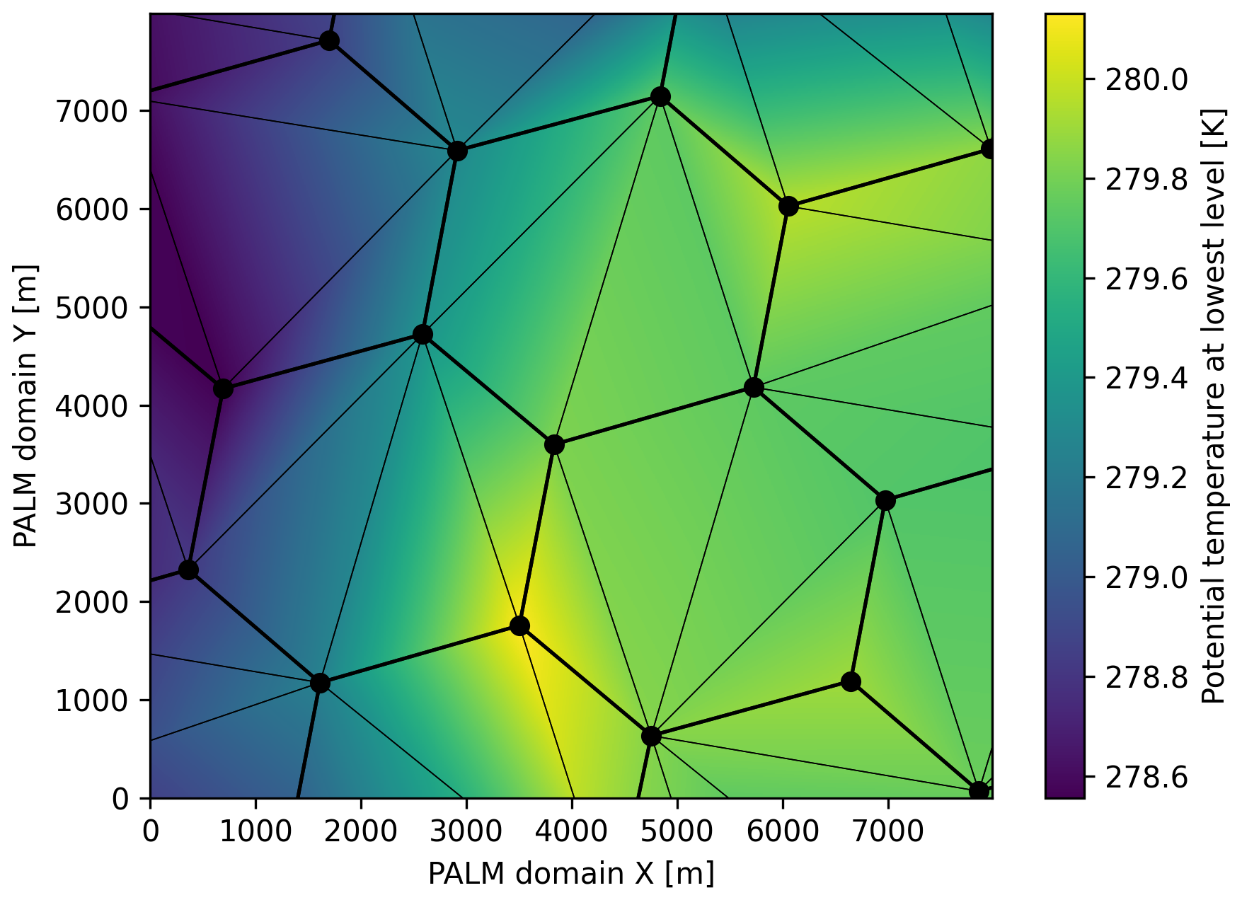
Figure 4 Demonstration of the barycentric horizontal interpolation for ICON-D2 data on the Legerova scenario (8 × 8 km from resolution approx. 2 km into 10 m; see Sect. 3.1). The black lines represent the triangulation of the source data points (black dots), and the fill is the interpolated field (near-surface potential air temperature). Note that the source data points are in a hexagonal pattern (the hexagons are accentuated with thicker lines), yet not perfectly regular (due to the projection of the icosahedral global grid); therefore, the triangulation of the individual hexagons is also irregular.

The DWD maintains an archive of ICON model data with multiple datasets from the ICON model analyses and forecasts. These datasets vary in the model variables they include and the duration for which they are kept in the archive. PALM-meteo can be used with both analysis and forecast data, but some DWD datasets do not contain all the variables required for PALM, such as the vertical velocity component.

The ICON variables, which remain constant for the duration of one forecast (one assimilation cycle), such as the vertical structure of the model levels, are included only in the first file for each forecast. PALM-meteo can be configured to generate a dynamic driver which spans multiple ICON forecasts as described in Sect. 2.2.1; in that case, it always loads the model level heights from the first (zero-horizon) file of each cycle, even if the specified earliest horizon is higher (i.e., the file is disregarded for other data).

Generating radiation inputs for PALM requires at least the shortwave and longwave horizontal irradiance, with an optional direct component for the shortwave irradiance. Unfortunately, most ICON outputs available from the DWD archive using PAMORE lack the downward longwave radiation, with only the net radiation available. Because the net radiation ${\mathrm{\Phi }}_{\mathrm{d}}=E_{\mathrm{e}}-J_{\mathrm{e}}$, where E_e is the received (downward) radiant flux and J_e is the leaving (upward) flux, PALM-meteo uses the Stefan–Boltzmann law to calculate the downward flux:

$$\begin{array}{}\text{(7)}& \begin{array}{rl}& {\mathrm{\Phi }}_{\mathrm{d}}=E_{\mathrm{e}}-J_{\mathrm{e}}=(E_{\mathrm{a}}+E_{\mathrm{r}})-(M_{\mathrm{e}}+E_{\mathrm{r}})=E_{\mathrm{a}}-M_{\mathrm{e}}\\ & {\mathrm{\Phi }}_{\mathrm{d}}=\mathit{\epsilon }{E}_{\mathrm{e}}-\mathit{\epsilon }\mathit{\sigma }{T}^{\mathrm{4}}\\ & E_{\mathrm{e}}={\displaystyle \frac{{\mathrm{\Phi }}_{\mathrm{d}}+\mathit{\epsilon }\mathit{\sigma }{T}^{\mathrm{4}}}{\mathit{\epsilon }}}\end{array}\end{array}$$

where E_a is the absorbed flux, E_r is the reflected flux, M_e is the emitted flux, ε is the surface emissivity, T is the surface temperature and σ is the Stefan–Boltzmann constant. All fluxes refer to the longwave band. The surface emissivity for each grid point in the ICON model is constant in time unless that area has snow cover (which is currently unsupported by PALM-meteo). It needs to be loaded from a separate file containing the static model fields.

2.3.6 Aladin

The Aladin (Aire Limitée Adaptation dynamique Développement InterNational) model was proposed by Météo-France in 1990 to build a mutually beneficial collaboration with the National Meteorological Services of Central and Eastern Europe. This collaboration results in Aladin running in operational mode in the Czech Hydrometeorological Institute (CHMI) and providing 3 d forecasts for a large part of Europe. The model assumes that the important meteorological events at those fine scales (local winds, breezes, thunderstorm lines, …) are mainly the result of a so-called “dynamical” adaptation to the characteristics of the Earth's surface. The model running at CHMI has a spatial resolution of 2.3 km in 87 vertical layers, coupling global models ARPEGE (Météo-France) and European Centre for Medium-Range Weather Forecasts' (ECMWF) Integrated Forecasting System (IFS). Since 2025, its results have been publicly available on the server https://opendata.chmi.cz (last access: 28 April 2026) with the metadata integrated within the National Open Data Catalogue (NKOD; Digital and Information Agency, 2025) and the geospatial data in the Czech National Geoportal INSPIRE (https://geoportal.gov.cz, last access: 28 April 2026).

The ALADIN plugin supports input files in the GRIB and GRIB2 formats. It was implemented with an extra data import step at the beginning, which converts the data into a temporary NetCDF file, which can save time when multiple datasets are prepared from the same inputs. In the future, this extra step will be eliminated.

The Aladin data from CHMI are provided on a regular grid in the LCC projection. PALM-meteo uses bilinear horizontal interpolation and supports also radiation inputs, including the direct component of the shortwave radiation. However, as these inputs are provided only at 1 h temporal resolution, the PALM simulations need to be monitored for artefacts related to the direct radiation near the horizon around sunrise and sunset.

2.3.7 CAMx

The CAMx plugin provides chemistry inputs from the CAMx chemical transport model. CAMx (Comprehensive Air Quality Model with Extensions) is a widely used Eulerian photochemical modelling system for gas and particulate air pollution. It allows for an integrated assessment of gaseous and particulate air pollution across many scales, from urban to regional. It has been developed since 1996 by Environ (currently part of the Ramboll company) under an open-source licence and has been employed extensively by government agencies, academic and research institutions, and private consultants for regulatory assessments and scientific research.

The CAMx model takes meteorological data from a meteorological model (e.g., WRF) and emission inputs provided by an emission modelling system (e.g., SMOKE or FUME) and provides fields of pollutant concentrations.

When the CAMx data is used in PALM-meteo, no assumptions are made about the relation between the meteorological and chemical inputs for PALM-meteo; therefore, PALM-meteo also supports the case where the CAMx model simulation was based on different meteorological inputs, and consequently on a different model grid. Still, if the configuration option camx:uses_wrf_lambert_grid is enabled, PALM-meteo assumes that the CAMx data are placed on a grid using the LCC projection from WRF (see Sect. 2.3.2 and interprets the projection metadata accordingly. In that case, it uses bilinear horizontal interpolation. If the option is disabled, PALM-meteo cannot make any assumptions about the model grid and the projection on which it is based, so it uses the latitude and longitude NetCDF variables for georeferencing input data, and it performs the barycentric interpolation on a triangulated grid as in ICON (Sect. 2.3.5).

The PALM chemistry module takes advantage of the Kinetic PreProcessor (KPP; see Damian et al., 2002), which offers multiple chemistry mechanisms with flexible configuration. As a result of that, the potential sets of IBC variables with chemistry species concentrations may be very different depending on the PALM KPP configuration, starting from simple passive tracer simulations with, e.g., aerosols (PM₁₀, PM_2.5) and/or typical pollutants (NO_x, SO₂) through mechanisms with simplified basic chemistry to very complex chemical mechanisms with tens of species, such as Carbon Bond 4 (CB4; see Gery et al., 1989).

The global or mesoscale chemical transport models may not always provide the exact set of concentration variables needed for PALM; often, it may be necessary to perform simple calculations such as unit conversions, summing up of species (e.g., NO_x from NO₂ + NO₃) or splitting by a ratio. PALM-meteo offers a flexible configuration system to specify chemical IBC species and to perform these calculations when required.

The main configuration for this purpose is the list of output chemical variables (empty by default when chemistry is disabled). Each output variable needs to have a definition with the list of input variables, the formula for calculating the output value from the input values, the output unit of the calculated value, and an optional list of assertions to be checked with the input variables. If the formulae for multiple variables contain an identical term, it is possible to configure it as a preprocessed value to avoid its repeated computation. Such definitions are provided for some commonly used chemical mechanisms (36 commonly used chemical species), but these can be easily extended and/or overwritten by the user. In addition to that, simple unit conversions are handled automatically as described in Sect. 2.2.6.

This configuration mechanism, which utilises different lists of predefined variables, is employed in all chemical plugins within PALM-meteo.

2.3.8 CAMS

Copernicus Atmosphere Monitoring Service (CAMS), and its implementation in the ECMWF's IFS, provides operational daily analysis and forecast of aerosol optical depth (AOD) for five aerosol species using an online integrated module for aerosol and chemistry coupled to IFS (C-IFS). A fully prognostic aerosol model has a significant impact on weather forecasts in cases of large aerosol concentrations, as observed during dust storms or intense pollution events.

The CAMS reanalysis datasets include: (i) the CAMS global reanalysis (EAC4), which currently covers the period from January 2003 to December 2024; (ii) and CAMS global greenhouse gas reanalysis (EGG4), which currently covers the period 2003–2020.

The CAMS reanalysis is the latest global reanalysis data set of atmospheric composition (AC) produced by the Copernicus Atmosphere Monitoring Service, consisting of 3-dimensional time-consistent AC fields, including aerosols, chemical species and greenhouse gases, through the separate CAMS global greenhouse gas reanalysis (EGG4). The data set builds on the experience gained during the production of the earlier MACC reanalysis and CAMS interim reanalysis.

The CAMS reanalysis was produced using 4DVar data assimilation in CY42R1 of ECMWF's IFS, with 60 hybrid sigma/pressure (model) levels in the vertical, with the top level at 0.1 hPa. Atmospheric data are available on these levels, and they are also interpolated to 25 pressure, 10 potential temperature and 1 potential vorticity level(s). “Surface or single-level” data are also available. Generally, the data are available at a sub-daily and monthly frequency and consist of analyses and 48 h forecasts, initialised daily from analyses at 00:00 UTC.

PALM-meteo supports CAMS outputs in the NetCDF format with the regular latitude–longitude grid (equirectangular projection). The mechanism for species calculations and unit conversions, as described in Sect. 2.3.7, is also used. The configuration is available for NO, NO₂, O₃, PM₁₀ and PM_2.5 and the postprocessing sum may be used to calculate NO_x.

2.3.9 Synthetic inputs

The synthetic input PALM-meteo plugin differs significantly from the other input plugins as it does not use meteorological data from any specific (mesoscale) model. Its goal is to enable simple and flexible creation of synthetic IBC by specifying vertical profiles and/or timeseries within the PALM-meteo configuration file, taking advantage of other PALM-meteo features, such as the vertical adaptation method (Sect. 2.2.3).

Vertical profiles of time-dependent variables can be set in the configuration section synthetic:prof_vars. A list of vertical profiles for velocity (u, v, w), potential temperature (θ), water vapour mixing ratio (q), soil temperature (t_soil) and moisture (q_soil) together with a list of heights for the profiles in meters above origin_z (or below for soil variables) can be prescribed.

Each vertical profile may be listed as constant or as a sequence of profiles with assigned times. In addition, the profiles in the sequence may be repeated and/or permuted by specifying their timeseries section, which simplifies creation of, e.g., multiple daily cycles.

This approach offers a more generic and flexible alternative to prescribing profiles via the PALM's PARIN (_p3d) namelist file. It enables time-dependent Dirichlet boundary conditions for all of u, v, w, θ, q and for the soil variables. Unlike PALM's built-in options set_constant_profiles and set_1d-model_profiles, this method offers more precise meteorological inputs, such as prescribing the full potential temperature profile rather than just setting a vertical gradient.

As the dynamic driver inputs are hydrostatic, pressure is prescribed as a single value; either for the surface pressure or the sea-level pressure, which is then converted to origin_z.

There is no verification whether the provided input data are physically consistent. Prescribing unrealistic values, such as large negative vertical gradients of θ, may lead to unrealistic or even crashed PALM simulations.

2.3.10 Wind damping near walls

Because the terrain matching and vertical adaptation method (Sect. 2.2.3) purposely ignores buildings and the mesoscale models in general cannot resolve such fine-scale details, the interpolated wind field for the initial conditions generated by PALM-meteo may contain a wind field that seems to enter and leave solid obstacles, thus creating velocity divergence. This is expected, and PALM solves this in its first timestep; however, it may negatively affect the convergence of the pressure solver, especially when the buildings contain narrow gaps which may not be (entirely) removed by PALM's terrain filtering.

PALM-meteo contains a plugin for damping the initial-condition wind near walls in a post-processing step. Depending on the configuration, it zeroes the U, V and W fluxes in one or more grid cells adjacent to the vertical walls and then linearly increases the wind damping factor from zero to one at a configured horizontal distance from the wall, from where onward the wind field remains unchanged. This process does not remove the velocity divergence of the initial wind field, but it has been tested to make the PALM's multigrid pressure solver converge faster.

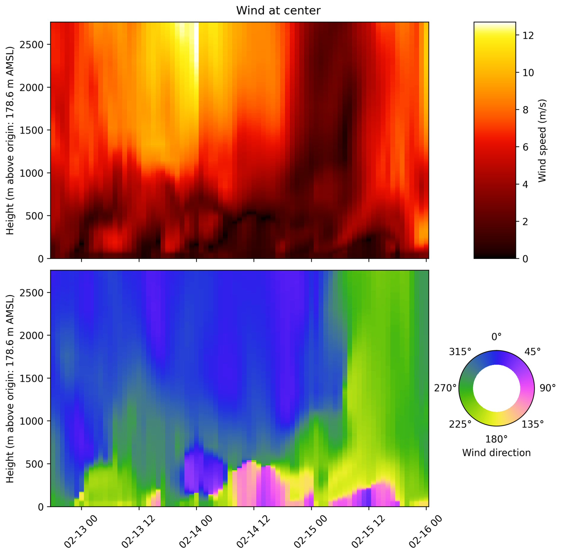
2.3.11 Vertical profile plotting

The plotting plugin generates graphical plots of any output variables (by default the wind speed + direction, potential temperature, and humidity). These plots are generated as heat maps with the y-axis representing height (above the origin height) for a selected location (centre of domain by default), the x-axis representing time and the colour representing the magnitude of the specific variable. They are useful for quick analysis of the meteorological inputs and their suitability for the intended PALM simulation, e.g. the wind speeds at all heights or the diurnal cycle of the convective boundary layer. The plots are generated at the write stage, utilising the full 3-D data for all times from the previous vertical interpolation stage. An example of wind speed and direction is available in Fig. 5.

Figure 5 Example output of the plotting plugin, showing wind speed and direction from the centre of the Legerova scenario (see Sect. 3.1).

3 Example use cases and performance

Since PALM-meteo is an input data processor for the PALM model, it can be evaluated indirectly by validating the result of the prepared PALM simulations and discussing the effect of IBC on the results.

PALM-meteo as well as its predecessor WRF_interface have already been used to generate meteorological inputs for PALM validation studies, such as Resler et al. (2021, 2024). Both studies mention strong dependence of PALM on driving meteorological conditions, where the errors in mescsale weather models used as inputs to PALM's IBC strongly influence the results of PALM simulations. A dedicated study on PALM's sensitivity to IBC using PALM meteo was performed by Radović et al. (2024). Section 1.5 describes this study and lists other studies using PALM-meteo. We consider these studies to be a sufficient evaluation of the results of PALM-meteo based PALM simulations. Consequently, this paper focuses more on PALM-meteo and its direct outputs.

To evaluate the computational requirements of PALM-meteo and to demonstrate its practical usability, two domains have been selected, one in Prague (Czech Republic) and one in Guelph (Canada).

3.1 Legerova (Prague, Czech Republic)

Prague is situated mainly on the Vltava River, and the Berounka River flows into the Vltava at the southern city border. Most of the city of Prague is located on the Prague plateau. In the south, the city's territory extends into the Hořovice Uplands, and in the north it extends into the Central Elbe Table lowland. The highest point is on the western border of Prague, at 399 m above sea level. Notable hills in the centre of Prague, rising from the Vltava river level, are Petřín with 327 m and Vítkov with 270 m. The lowest point is the Vltava in Suchdol where it leaves the city, at 172 m. With an elevation range around 230 m, Prague represents a complex urban landscape including steep hills and deep valleys (see Fig. 6).

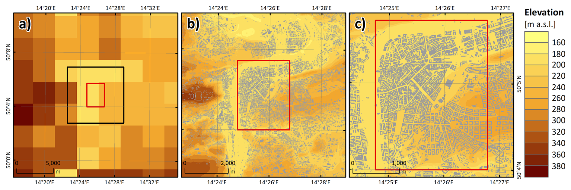
Figure 6 Example of the domain centred on Legerova street (Prague, Czech Republic) with a digital elevation model in resolution of 3 km (a), 8 m (b) and 2 m (c). The black square represents a parent domain, and the red square the asymmetrically located child domain.

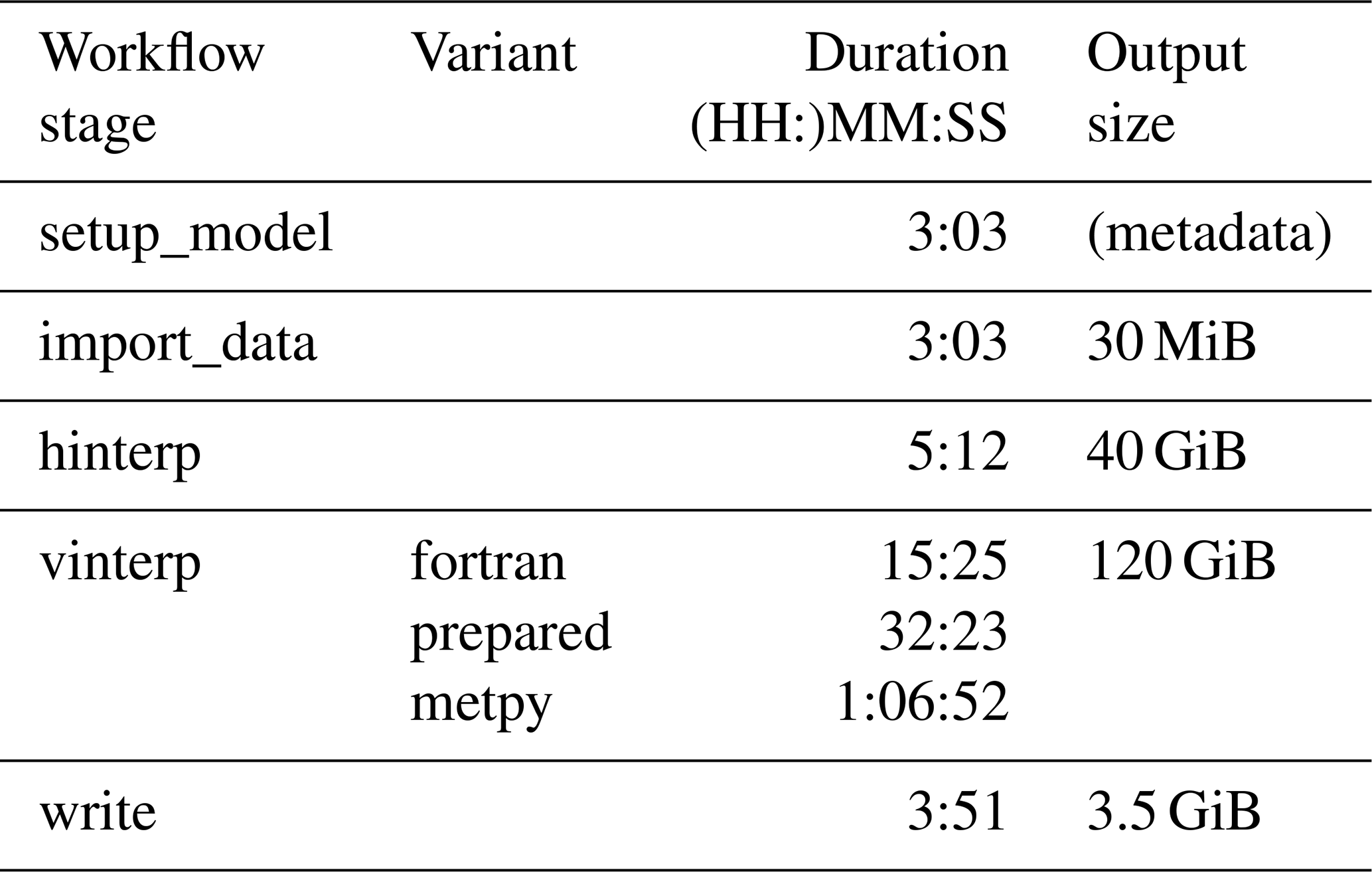
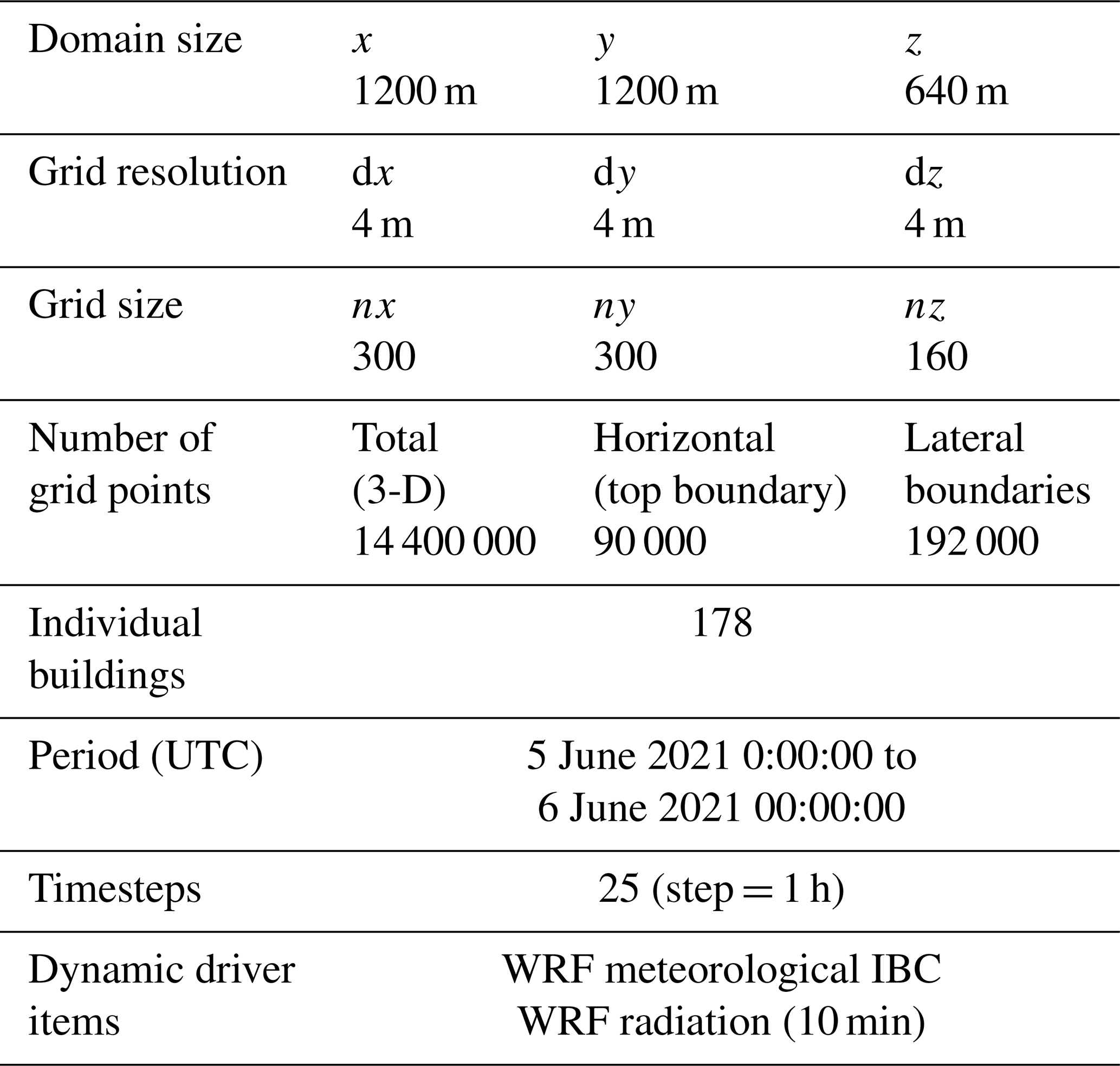
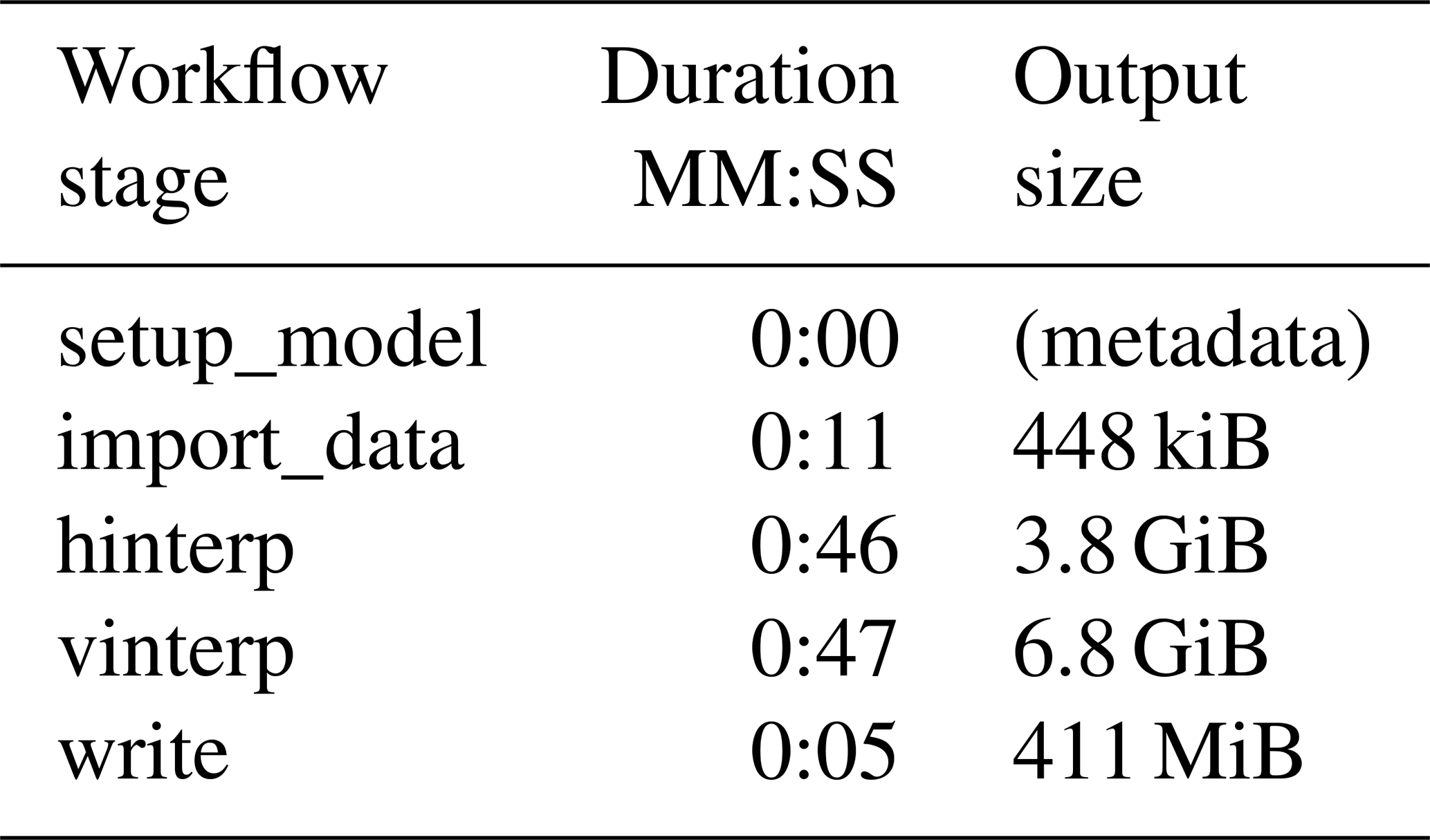
The parameters of the Legerova simulation domain are listed in Table 1. The times needed for the full PALM-meteo workflow in the parent domain (which contains both initial and boundary conditions, as opposed to the dynamic driver for the child domain with only initial conditions), running on the Intel Xeon Gold 6242 CPU, are listed in Table 2. The total processing took 31 min with the fortran vertical interpolator.

Table 1 Parameters of the Legerova simulation (parent domain).

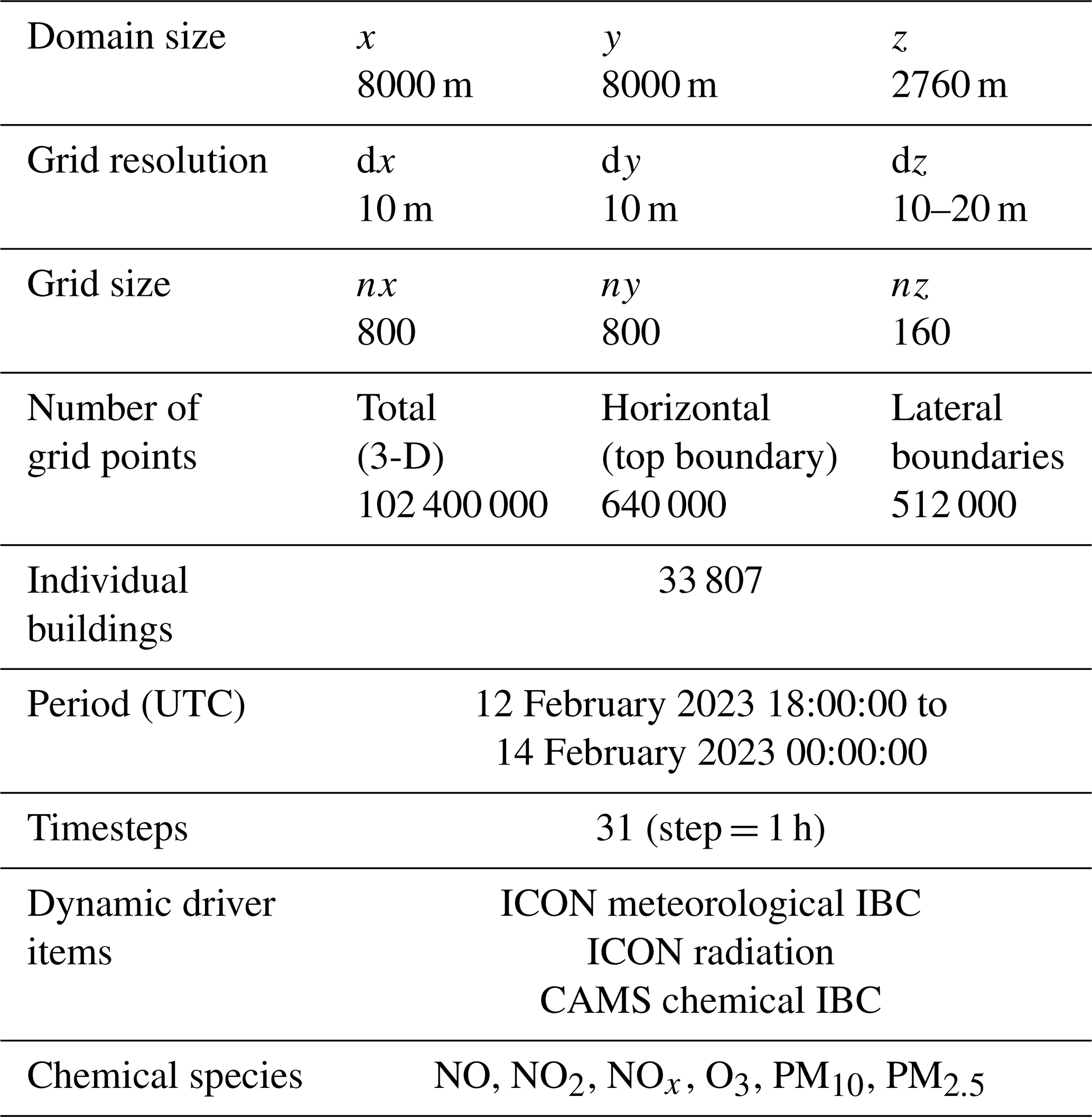
Table 2 Performance of PALM-meteo on the Legerova parent domain.

An example of the wind component perpendicular to the domain border processed from meteorological data provided by three different mesoscale models is shown in Fig. 7.

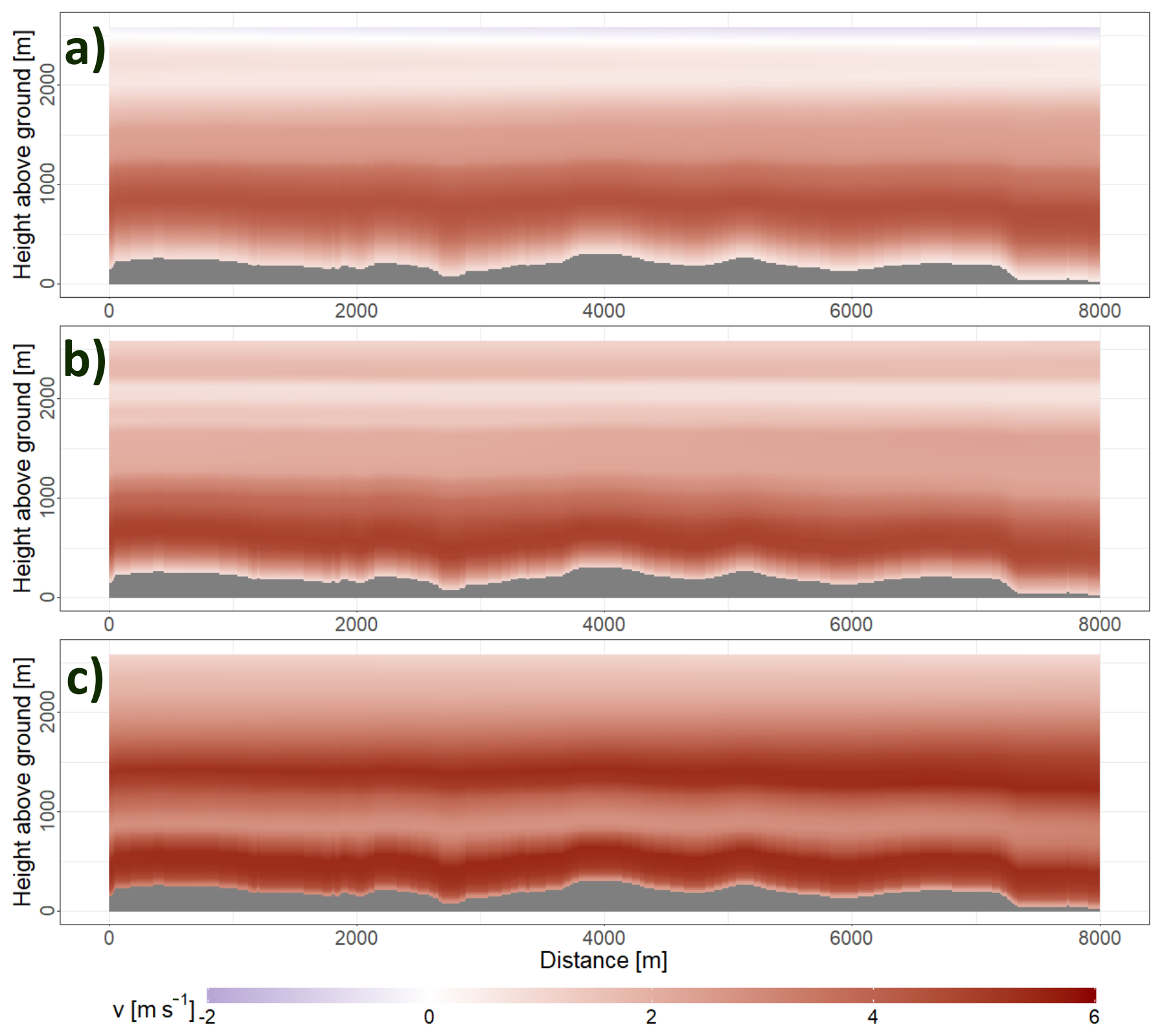
Figure 7 Example of the u component of wind on the Eastern boundary of the Legerova domain (Prague, Czech Republic) processed from Aladin (a), ICON (b), and WRF (c) meteorological models on 13 February 2023 at 09:00 UTC.

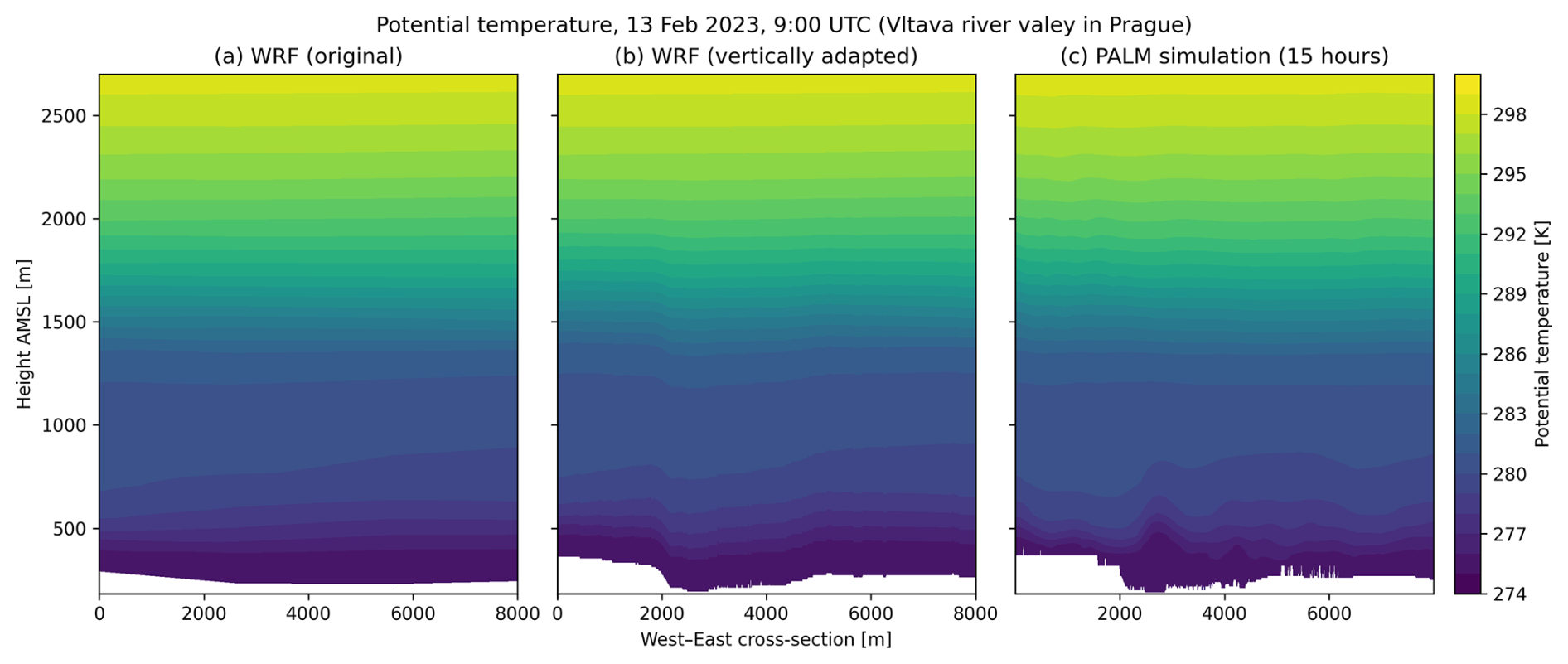
Figure 8 Comparison of vertical cross-section of potential temperature from the original WRF data (a), vertically adapted PALM-meteo outputs (b) and the outputs from a PALM simulation driven by those IBC (c). The PALM simulation started 15 h prior to the displayed time. The position and time of the cross-section matches Fig. 3 in Sect. 2.2.3.

Figure 8 illustrates the processing from a different point of view. It compares the potential temperature from the original WRF outputs, the same values vertically adapted by PALM-meteo to match the terrain (see also Sect. 2.2.3) and the values from the actual PALM simulation which was driven by those meteorological inputs.

This sequence demonstrates that the original vertical levels from WRF were based on a coarse terrain that was inconsistent with the high resolution terrain in PALM, so they needed to be adapted by PALM-meteo. In this case, the adaptation was configured with the transition level 2000 m above origin_z. The vertical shifts are still apparent around 1300 m a.m.s.l., yet the PALM simulation driven by these inputs maintains relatively flat layers of potential temperature above approximately 1000 m. The current version of PALM-meteo has the default transition level set to 300 m above the highest obstacles, which further decreases the vertical propagation of the terrain following structures.

3.2 Guelph (Ontario, Canada)

Guelph is situated above the confluence of the Speed River and the Eramosa River. The Speed River enters from the north and the Eramosa River from the east; the two rivers meet below downtown and continue southwest, where they merge with the Grand River (Ontario). The landscape was heavily sculpted by glaciers, and the terrain is mostly flat, with old river mounds. The mean elevation is 33 m, and the difference between the lowest and highest point is less than 50 m. The Guelph terrain elevation in different domains of different resolutions is shown in Fig. 9.

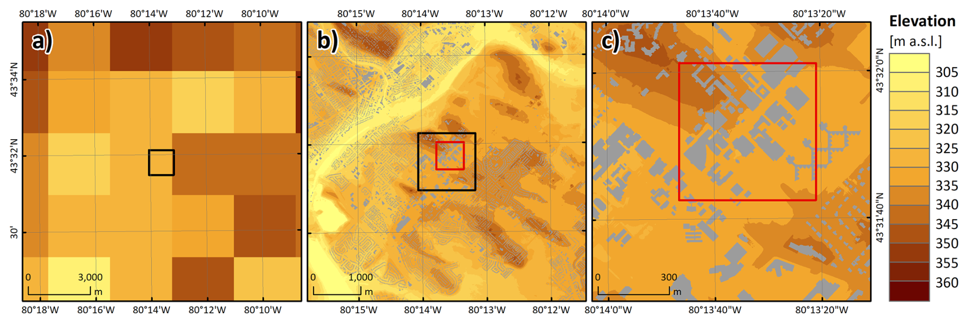
Figure 9 Example of the asymmetrically located domain centred on campus of the University of Guelph (Ontario, Canada) with a digital elevation model in resolution of 3 km (a), 8 m (b) and 1 m (c). The black square represents a parent domain, and the red square the asymmetrically located child domain.

The parameters of the Guelph simulation domain are listed in Table 3. The times needed for the full PALM-meteo workflow in the parent domain, running on the Intel Xeon Gold 6242 CPU, are listed in Table 4. Since the domain is a lot smaller than the Legerova domain and there are no chemical variables, the total processing took only 1 min 49 s. This processing used only the preferred fortran vertical interpolator.

Table 3 Parameters of the Guelph simulation (parent domain).

Table 4 Performance of PALM-meteo on the Guelph parent domain.

4 Conclusions and further work

This paper thoroughly describes the PALM-meteo tool, its architecture, and its applicability for preparing meteorological inputs for the PALM model, together with example applications.

PALM-meteo significantly extends the scope of usable meteorological inputs for the PALM model. Its focus on flexibility, modularity and extensibility, together with decent performance, allows it to be continuously improved and thoroughly verified at each stage of its processing. Its applicability for realistic PALM simulations has already been demonstrated by previously published studies mentioned in Sect. 1.5.

PALM-meteo continues to be under active development, with new plugins being added and the program core and currently available modules being improved and optimised.

New plugins are currently being developed for the ALARO, HARMONIE and WRF-Chem models. Further plugins are currently being considered for the GFS model outputs and ERA reanalyses. There is also an ongoing general effort towards further deduplication and modularisation of tasks within the current plugins.

Appendix A: PALM-meteo implementation

A1 Plugin system

PALM-meteo is designed from the ground up to be modular and extensible, so that adding plugins that support new input formats and data sources is as easy as possible.

The core of the program resides in the Python module palmmeteo. The basic set of plugins provided with PALM-meteo is packaged in the module palmmeteo_stdplugins. User-supplied plugins are expected to be placed in modules whose names start with the prefix palmmeteo_. Each plugin – standard or user-supplied – can implement one or more stages (see Sect. 2.1). This is done by implementing a class derived from palmmeteo.plugins.Plugin and the respective abstract base classes, such as palmmeteo.plugins.ImportPluginMixin, or alternatively by using the function decorator palmmeteo.plugins.eventhandler.

A2 Configuration system

The configuration of PALM-meteo is represented as a tree-like structure where internal nodes are either dictionaries or ordered lists, and the leaf nodes are values of various data types. This is a common structure which matches, e.g., JSON or YAML files.

Although it is possible to run PALM-meteo with only a few lines of configuration (keeping defaults for the rest), the full documentation tree contains a variety of values ranging from mandatory user-specified configuration to the programmer-specified constants, with a marginal chance of ever having to be altered. PALM-meteo does not draw a strict boundary between beginner-, advanced- or programmer-specific configuration. The user-facing options are well documented, and an example of their usage is provided in the template configuration file. Advanced users or programmers, and debuggers may also alter the non-documented configuration options; it is their responsibility to edit only the values they fully understand.

A2.1 Tasks

To make the basic configuration easier, PALM-meteo uses large chunks of configuration called tasks. A single configured job for PALM-meteo may contain one or more tasks, each of which enables a logical, mostly self-contained chunk of processing, such as taking meteorological inputs from a specific mesoscale model. A single task typically enables one or more plugins and sets the related initial configuration, which can be further modified by the user's config file(s).

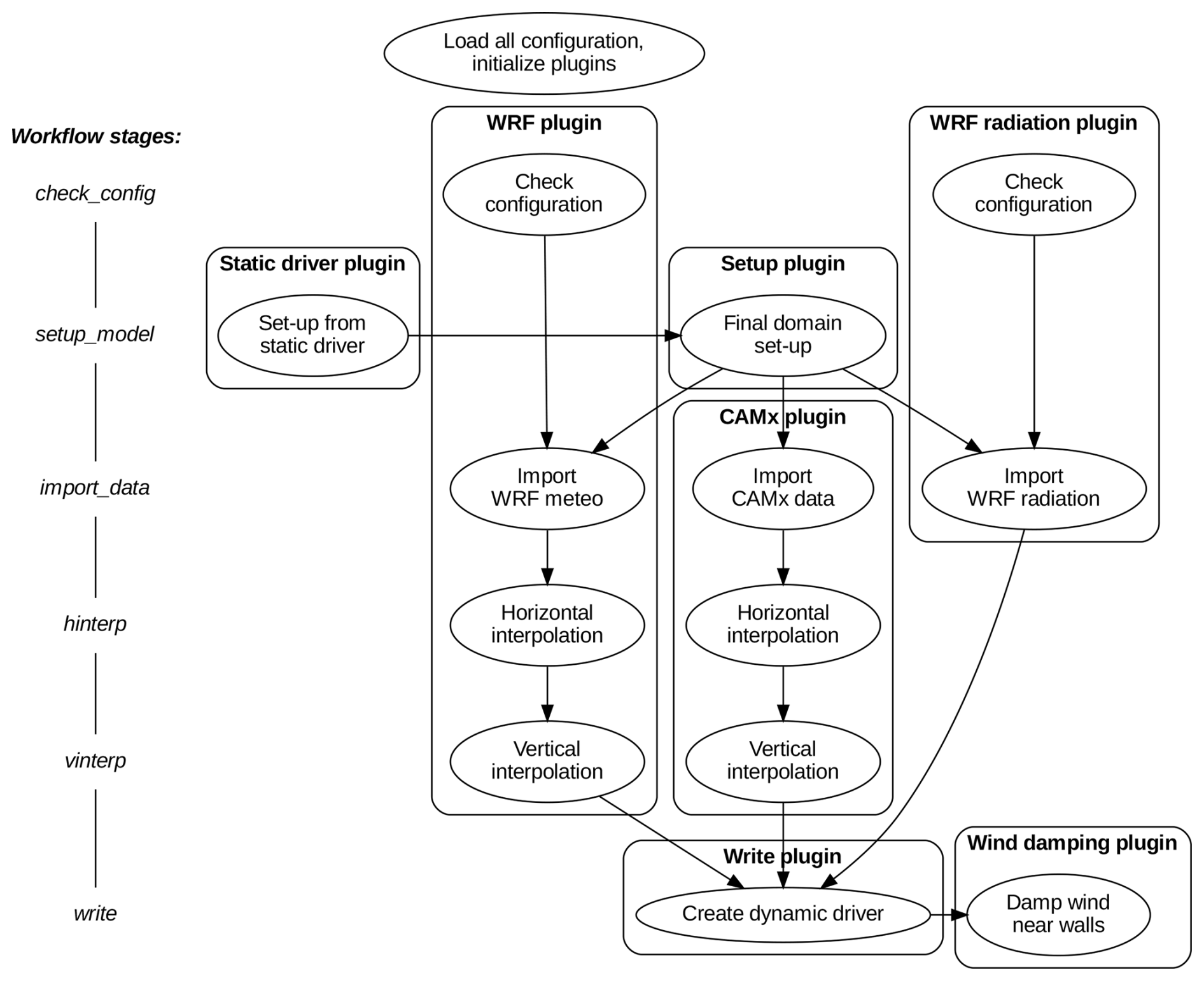
Figure A1 A flowchart of processing of an example PALM-meteo scenario with multiple plugins for meteorological and chemical IBC, including radiative forcing.

The current version of PALM-meteo contains these tasks:

wrf:

Loads meteorological inputs from the WRF model.

wrf_rad:

Loads radiation data from the WRF model and includes them in the output dynamic driver. These are independent of the basic meteorological inputs (atmosphere and soil), which may come from a different model.

icon:

Loads meteorological inputs from the ICON model. Radiation data may be included if configured.

aladin:

Loads meteorological inputs from the Aladin model.

aladin_rad:

Loads radiation data from the Aladin model (independent of the basic meteorological inputs).

camx:

Loads chemistry data from the CAMx model.

cams:

Loads chemistry data from the CAMS model.

synthetic:

Specifies basic meteorological inputs using specified constants, profiles and timeseries, so that no mesoscale weather model data are necessary.

winddamp:

Performs damping of the wind ($u,v,w$) near vertical walls in the initial conditions.

plot:

Generates graphical plots of selected output variables.

From the configuration point of view, each task specifies a sub-tree which will be applied over the main configuration tree if the specific task is enabled. This is applied after loading the user configuration, and the values which are already specified by the user are not overwritten.

An example of a complete processing workflow of a PALM-meteo scenario with multiple plugins is presented in Fig. A1. This scenario used the tasks wrf, wrf_rad, camx, and winddamp, which enabled the respective plugins in addition to the plugins enabled by default (Static driver, Setup, and Write).

A2.2 Configuration processing

PALM-meteo assembles the full documentation tree from several fragments loaded from separate YAML files. The initial default values are loaded from the YAML files shipped with the source code, and the user values from the user-supplied configuration file(s). The configuration is processed in five steps:

1. Default values for core options from the core configuration default file.

2. Default values for plugin-specific options from the plugin configuration default files (overwriting previous values in case of conflict).

3. Configuration from the user configuration file is loaded and applied (overwriting defaults). If there is more than one configuration file specified, they are applied in the specified order (overwriting previous values).

4. For each enabled task, the configuration sub-tree of that task is applied over the configuration tree (non-overwriting).

5. Command-line options are applied to the respective configuration values (overwriting).