Love number computation within the Ice-sheet and Sea-level System Model (ISSM v4.24)

The Love number solver presented here is a new capability within the Ice-sheet and Sea-level System Model (ISSM) for computing the response of a 1D radially-symmetric solid Earth to tidal forcing and surface mass loading. This new capability allows solving zero-frequency free oscillation equations of motion decomposed into the well-known y_i system and enables high wave number computations with spherical harmonic truncation degree of ∼ 10 000 and above. It facilitates capturing the high-resolution response of the solid Earth to a step-function forcing in terms of gravity potential changes, vertical and horizontal bedrock displacement, and polar motion. The model incorporates compressible isotropic elasticity and three forms of linear viscoelasticity for mantle rheology: the Maxwell, Burgers, and Extended Burgers Materials (EBM). We detail our approach to the parallelization and numerical optimization of the solver, and report the accuracy of our results with respect to community benchmark solutions. Our main motivation is to facilitate simulations of a coupled system of surface mass transport (e.g. changes in polar ice sheets and sea level) and solid Earth models at kilometer-scale lateral resolutions with numerical efficiency that supports the exploration of large model ensembles and uncertainty quantification.

1 Introduction

1.1 General context

The viscoelastic solid-Earth and sea level response to the redistribution of surface mass in the cryosphere, ocean, terrestrial water and sediments has a numerical modeling history of nearly six decades (McConnell, 1965; Peltier, 1974). This response is typically expressed in terms of bedrock deformation, changes in relative sea level, gravitational potential, geocentric motion, and Earth's rotation parameters. These are collectively referred to as the Gravity, Rotation and Deformation (GRD) signals (Gregory et al., 2019). GRD models have been used in problems where the loading time scale ranges from thousands of years (often referred to as Glacial Isostatic Adjustment or GIA, Whitehouse, 2018) to sub-seasonal (e.g. Adhikari et al., 2019; Michel and Boy, 2022; Heki and Jin, 2023), and applied on regional (e.g. Yousefi et al., 2018; Wake et al., 2016; Spada and Melini, 2022) to global scales (Peltier et al., 2015; Caron et al., 2018; Gowan et al., 2021). As such, GRD models have proven instrumental in better interpreting the signals recorded in geologic and geodetic data, such as past sea level indicators, tide gauges, Global Navigation Satellite Systems (GNSS), terrestrial and space gravimetry, and satellite altimetry. Outstanding differences between GRD models generally stem from three distinct sources (e.g. Caron et al., 2018; Melini and Spada, 2019; Cederberg et al., 2023): (1) the selection and curation of constraining datasets; (2) treatment of solid Earth structure and mantle rheology; and (3) various refinements to the loading history. The presented Love number solver enables systematic investigation of model disparities related to the radial solid-Earth structure and mantle rheology.

The emergence of modeling approaches that couple ice sheet dynamics with GRD processes has revealed important feedback mechanisms impacting the grounding line migration and marine ice sheet instability on decadal and longer timescales (e.g. Gomez et al., 2015; Larour et al., 2019; Book et al., 2022). Our main motivation is to enable the Ice-sheet and Sea-level System Model (ISSM) to tackle such coupled problems and enhance its sea-level projections framework (Adhikari et al., 2016; Larour et al., 2020). Our capability is also adapted to lower complexity models wherein the ice history is prescribed a priori (e.g. using the ICE-6G model from Peltier et al., 2015), which may be considered as a one-way coupling problem.

In this paper, we document the recently-coded Love number solver in the ISSM framework (Caron, 2024, available at https://doi.org/10.5281/zenodo.13984073), capable of accounting for a range of linear viscoelastic rheologies for the mantle and lithosphere. We report our numerical approach and optimization strategy. By employing higher-order linear viscoelasticity that predicts rapid deformation at short time scales (e.g. Faul and Jackson, 2015; Hazzard et al., 2023; Ivins et al., 2023a), this new ISSM capability may be used to examine rapid ice sheet-solid Earth interactions on time scales of months to decades. The capability also facilitates studying general interactions between the Hydrosphere and Solid Earth as well as GRD phenomena in other planetary bodies. It may also be adapted to investigate a host of problems involving tidal dispersion and dissipation in Earth and elsewhere.

1.2 Spherically symmetric vs 3D Earth model for GRD

New model approaches that deviate from the surface load Love number formulation are used to include a laterally variable Earth rheology (Latychev et al., 2005; Zhong et al., 2022; Lloyd et al., 2024; Huang et al., 2023; van Calcar et al., 2023). These new methods combine prior information on the radial dependence of mantle rheology with lateral viscosity contrast estimated from seismic velocity anomalies. While poised to become the standard in GRD modeling at sometime in the future, 3D Earth GRD models are computationally costly compared to approaches that approximate the Earth structure to be only radially dependent, a necessary ingredient of the Love number approach. This currently limits our ability to evaluate uncertainty on Earth parameters. We note that potential solutions are explored in the community in the form of emulators (Lin et al., 2023; Love et al., 2024) and sensitivity kernels (Lloyd et al., 2024). Love number approaches still remain a powerful method to explore the background rheology profile, and to establish a robust prior for its parameters (Caron et al., 2017; Melini and Spada, 2019) owing to their low computational cost. This is particularly beneficial for frameworks that rely on ensemble modeling to comprehensively approach interdisciplinary problems such as projections of sea-level change (Larour et al., 2020). Recent improvements to the theory and numerical implementation of the Love number problem include new approaches to time-dependent response to tidal and surface loading (Martinec and Hagedoorn, 2014; Melini et al., 2022; Michel and Boy, 2022) as well as rigorously accounting for the adiabaticity of mantle thermal structure (Kachuck and Cathles, 2019). Furthermore, a new formulation of a linear rheology, the Extended Burgers rheology (EBM), featuring both transient and steady-state relaxation, have been documented by Faul and Jackson (2015), Simon et al. (2022), Ivins et al. (2022, 2023a), Lau (2023). Work parallel to our new ISSM core has recently been published by Lau (2024) who also solves the Love number problem with a higher-order linear viscoelasticity. The latter work does not pursue EBM rheology, but rather a structurally similar formulation developed by Yamauchi and Takei (2016) based upon experiments with granular borneol. Lau (2024), and the work presented here, represent a new and exciting direction for radially stratified models of GRD processes that occur during the Little Ice Age and Anthropocene and that should be included in solid Earth-ice interaction models of future sea-level change. As these new rheological models emerge, we believe that it is first important to understand what observational constraints can be put on transient relaxation parameters at the lowest level of model complexity.

1.3 Transient mantle rheology

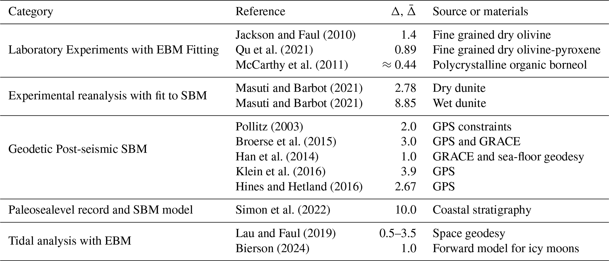
One of the traditional goals of GIA modeling is to determine the spatial dependence of the effective Newtonian viscosity that characterizes the mantle circulation time scales (t≥10 million years, e.g. Hager and Clayton, 1989; Mitrovica and Forte, 2004). While Lau et al. (2020) have recently pointed out that an improved reconciliation among various inferences of lithospheric thicknesses over ten thousand to hundred million year time scales may be achieved by invoking frequency dependent rheology, there is general consensus on the internal consistency of sub-lithospheric viscosity structure based on both GIA and mantle convection. However, geodetic observations of load-related vertical motions of the crust following load changes during the past 100 years suggest much lower values of the effective viscosity (e.g. Nield et al., 2014; Kierulf et al., 2022) and this may be related to the fact that this short time-scale is not recording information about long-term viscosity (e.g. Hazzard et al., 2023; Kierulf et al., 2022). More convincing evidence for transient rheology comes from the geodetic observations of time-dependent, widespread crustal motions following large earthquakes. The later observations have been modeled using the simple Burgers rheology, from which a value of the amplitude factor $\overline{\mathrm{\Delta }}$ may be deduced. By using the linear constitutive EBM equations that have been proposed to explain laboratory experimental data (e.g. Faul and Jackson, 2015) we may employ parameter values that are consistent with either post-seismic studies of high temperature and pressure laboratory studies, or to both. In Table 1 we present some of the values of the transient relaxation strength parameter from tidal, post-seismic and laboratory experiments for both $\overline{\mathrm{\Delta }}$ and Δ.

Jackson and Faul (2010)Qu et al. (2021)McCarthy et al. (2011)Masuti and Barbot (2021)Masuti and Barbot (2021)Pollitz (2003)Broerse et al. (2015)Han et al. (2014)Klein et al. (2016)Hines and Hetland (2016)Simon et al. (2022)Lau and Faul (2019)Bierson (2024)

Table 1 Estimates of transient relaxation strength Δ. [1]: Reported ratios of relaxed and unrelaxed Young's modulus. SBM: Simple Burgers Material. EBM: Extended Burgers Material.

Transient rheology may also be necessary to explain time-varying features of geodesy that are global in scale, such as the ongoing changes in the Earth shape, $\dot{J_{\mathrm{2}}}$ (e.g. Métivier et al., 2020). At a global scale there exist abundant information associated with the response of the Earth to body tides. Theories for the frequency-dependent dissipative processes interior to planet-moon systems have long been sought to reconcile the astronomically based necessity of low Q/high dispersion with high temperature and pressure laboratory data (e.g. Goldreich, 1963; Goldreich and Soter, 1966). Over the past 50 years a frequency-dependent Andrade rheology has been employed in the study of planetary Q (e.g. Castillo-Rogez et al., 2011). However, it has become clear that EBM models are also applicable to the study of tidal dispersion and dissipation (e.g. Lau and Faul, 2019; Gevorgyan et al., 2020; Bierson, 2024). Therefore, our new ISSM Love number computational capability can also support the development of planetary interior models that satisfy tidal observations and simultaneously provide prediction of a long-term viscosity.

A basic assertion of the Andrade model is that the creep function takes a form that includes a term with time-dependence, βtⁿ, with $n\approx \mathrm{1}/\mathrm{3}$ and β a coefficient (e.g. Cooper, 2002). Hence, developing models consistent with a long-term viscosity are excluded. One of our future goals will be to couple ice sheet grounding line evolution to motions of the bedrock topography, as the latter influence ice sheet mass balance projections, and as such, the coupled ice sheet model may require updating solid Earth viscoelastic response on a sub annual time scale. In such models it will be important to have a reference long-term viscosity incorporated into the model. In summary, EBM models find support from models of both post-seismic geodetic observations (Pollitz et al., 2006), terrestrial and planetary tides and may additionally be connected to long-term viscosity inferences (e.g. Whitehouse et al., 2019; Ivins et al., 2023b; Hazzard et al., 2023).

1.4 Main goals

Our main focus in this paper is to develop a toolset that enables the coupling of surface mass transport models (e.g. ice flow models) and GRD models with a variety of linear rheologies. Thus, our GRD model uses a Love number framework with radially symmetric Earth representation. Specifically, we target the following key capabilities for our solver:

1. The Love numbers are expressed as the time-dependent response to a Heaviside forcing function, thus facilitating the coupling with surface mass transport model through an explicit time-stepping framework.

2. The solver must support the computation of the Love number system at very high spherical harmonic degree (>10⁴). This requirement follows from the results suggested by Larour et al. (2019), wherein localizing ice changes and solid-Earth deformation was found to be important at kilometer scale, the same scale over which basal topography beneath the ice sheet exhibits flow inhibiting/promoting variability.

3. The solver must support the computation of compressible linear viscoelastic rheologies for the mantle, including support for transient relaxation. This follows some of the latest advances in modeling the mantle mechanics (Ivins et al., 2020, 2022, 2023a; Lau and Faul, 2019; Lau et al., 2021) for properly characterizing the time scale over which ice evolution occurs in the presence of complex underlying topography.

4. The solver must be computationally efficient enough to allow for the rheological parameter space to be explored using ensemble modeling approaches and Bayesian explorations. Considerable uncertainty remains in GIA and surface loading models, thus proper characterization of the non-uniqueness of the model solutions has proven critical to evaluate applications to geodetic datasets (Caron et al., 2018) and projections (Larour et al., 2020).

In the following sections we lay out the theory underlying the Love number system, explain our approach to both implementing and optimizing the numerical resolution of that system, and assess the efficiency and accuracy of our solver with respect to the community benchmark of Spada et al. (2011).

Table 2 List of symbols commonly used in this paper.

2 Theory

The classical problem of the Earth’s deformation in the presence of either discrete or continuous loading for a spherical self-gravitating sphere with a mantle and a liquid core has been formulated and solved for more than a century (Herglotz, 1905; Love, 1911). However, it was only with the development of modern computational physics that practical solutions to this fundamental solid Earth boundary value problem were realized (Pekeris and Jarosch, 1958; Alterman et al., 1959). We begin our discussion with the basic equations of motion and gravitation along with the relevant independent and dependent variables in this mathematical system.

2.1 Physics and Perturbation Equations

At the heart of the Love number problem is an ordinary differential equation system first described in its viscoelastic form by Peltier (1974). It is derived by combination of equations governing the conservation of mass and linear momentum and Poisson's equation:

$$\begin{array}{}\text{(1)}& {\displaystyle \frac{\partial \mathit{\rho }}{\partial t}}=-\mathrm{\nabla }\cdot \left(\mathit{\rho }\overline{\mathit{u}}\right)\text{(2)}& {\displaystyle }\mathit{\rho }{\displaystyle \frac{{\partial }^{\mathrm{2}}\overline{\mathit{u}}}{\partial t^{\mathrm{2}}}}=\mathrm{\nabla }\cdot \overline{\overline{\mathbf{\Sigma }}}+\mathit{\rho }\mathrm{\nabla }({\mathrm{\Phi }}_{\mathrm{E}}+S)\text{(3)}& {\displaystyle }\mathrm{\Delta }{\mathrm{\Phi }}_{\mathrm{E}}=-\mathrm{4}\mathit{\pi }G\mathit{\rho }\end{array}$$

Here $\overline{\mathit{u}}$ represents the displacement vector of solid-Earth material at any location, Φ_E the Earth's gravity potential (excluding any surface loading), ρ is the solid-Earth material density, $\overline{\overline{\mathbf{\Sigma }}}$ is the stress tensor, S is the gravity potential of the external forcing, G is Newton's gravitational constant and and t the time coordinate (see Table  for the list of symbols used in this paper). In these balance equations we include both the perturbed and unperturbed states, respectively indicated with subscripts 1 and 0. The unperturbed state balance is:

$$\begin{array}{}\text{(4)}& \mathrm{\nabla }{\mathcal{P}}_{\mathrm{0}}\left(r\right)=-{\mathit{\rho }}_{\mathrm{0}}\left(r\right)g_{\mathrm{0}}\left(r\right){\overline{\mathit{e}}}_{\mathrm{r}}\end{array}$$

for the spherically symmetric static Earth, with 𝒫₀, ρ₀ and g₀ representing the hydrostatic pressure, density and gravity, r the radius variable and ${\overline{\mathit{e}}}_{\mathrm{r}}$ the unit vector in the radial direction. The model static potential is

$$\begin{array}{}\text{(5)}& {\mathrm{\nabla }}^{\mathrm{2}}{\mathrm{\Phi }}_{\mathrm{E}\mathrm{0}}\left(r\right)=-\mathrm{4}\mathit{\pi }G{\mathit{\rho }}_{\mathrm{0}}\left(r\right)\end{array}$$

where we define the separation of total potential by

$$\begin{array}{}\text{(6)}& {\mathrm{\Phi }}_{\mathrm{E}}={\mathrm{\Phi }}_{\mathrm{E}\mathrm{0}}\left(r\right)+{\mathrm{\Phi }}_{\mathrm{E}\mathrm{1}}(t,r,\mathit{\theta },\mathit{\phi })\end{array}$$

and density by

$$\begin{array}{}\text{(7)}& \mathit{\rho }={\mathit{\rho }}_{\mathrm{0}}\left(r\right)+{\mathit{\rho }}_{\mathrm{1}}(t,r,\mathit{\theta },\mathit{\phi }).\end{array}$$

Here perturbed variables Φ_E1 and ρ₁ represent small anomalies to the unperturbed state induced by the forcing. Note that Eqs. (5) and (6) may be used to construct viscoelastic models for any terrestrial-like planetary body. We also note that the unperturbed gravity may be constructed from:

$$\begin{array}{}\text{(8)}& g_{\mathrm{0}}\left(r\right)={\displaystyle \frac{\mathrm{4}\mathit{\pi }G}{r^{\mathrm{2}}}}\underset{\mathrm{0}}{\overset{r}{\int }}{r^{\prime }}^{\mathrm{2}}{\mathit{\rho }}_{\mathrm{0}}\left(r^{\prime }\right)d{r}^{\prime },\end{array}$$

with G Newton's gravitational constant. Furthermore, the perturbed density is also recoverable from the mass conservation equation as

$$\begin{array}{}\text{(9)}& {\mathit{\rho }}_{\mathrm{1}}=-{\mathit{\rho }}_{\mathrm{0}}\mathrm{\nabla }\cdot \overline{\mathit{u}}-\overline{\mathit{u}}\cdot \left({\displaystyle \frac{\partial {\mathit{\rho }}_{\mathrm{0}}}{\partial r}}\right){\overline{\mathit{e}}}_{\mathrm{r}}.\end{array}$$

For brevity we shall drop the subscript “1” from ρ₁ in what follows. For completeness we also note that the perturbed pressure field is

$$\begin{array}{}\text{(10)}& {\mathcal{P}}_{\mathrm{1}}={\mathit{\rho }}_{\mathrm{0}}\left(r\right)g_{\mathrm{0}}\left(r\right)\overline{\mathit{u}}\cdot {\overline{\mathit{e}}}_{\mathrm{r}}.\end{array}$$

Note that we have yet to specify the relationship between $\overline{\overline{\mathbf{\Sigma }}}$ and $\overline{\mathit{u}}$ as it depends on the choice of rheological model employed for solid Earth material.

The problem is simplified by two approximations. First, the deformation regime is considered to be limited to small pertubations of the system, i.e. cross-terms δuδv can be neglected in expressions with the form $u.v=(u_{\mathrm{0}}+\mathit{\delta }u)(v_{\mathrm{0}}+\mathit{\delta }v)=u_{\mathrm{0}}{v}_{\mathrm{0}}+u_{\mathrm{0}}\mathit{\delta }v+v_{\mathrm{0}}\mathit{\delta }u+\mathit{\delta }u\mathit{\delta }v$, wherein u₀ and v₀ refer to variables (displacement, gravity potential, density, etc) in the initial state of the system. Second, the Earth structure is assumed to be radially symmetric (i.e. with no lateral variations) and the material to be isotropic.

2.2 Spectral Expansion

The full system of perturbation equations is fully derived by Gilbert and Backus (1968). The resulting system involves 6 radially-dependent variables (and their first radial derivatives) conventionally noted y_i(r) for $\mathrm{1}<i<\mathrm{6}$ (Alterman et al., 1959):

$$\begin{array}{}\text{(11)}& {\displaystyle }\begin{array}{rl}\overline{\mathit{u}}(r,\mathit{\theta },\mathit{\phi },t)& =a\sum _{n=\mathrm{1}}^{n_{max}}\sum _{m=\mathrm{0}}^n{y}_{\mathrm{1},n}(r,t)Y_n^m(\mathit{\theta },\mathit{\phi }){\overline{\mathit{e}}}_{\mathrm{r}}+y_{\mathrm{3},n}(r,t)\\ & \left({\displaystyle \frac{\partial Y_n^m(\mathit{\theta },\mathit{\phi })}{\partial \mathit{\theta }}}{\overline{\mathit{e}}}_{\mathit{\theta }}+{\displaystyle \frac{\partial Y_n^m(\mathit{\theta },\mathit{\phi })}{\sin \mathit{\theta }\partial \mathit{\phi }}}{\overline{\mathit{e}}}_{\mathit{\phi }}\right),\end{array}\text{(12)}& {\displaystyle }\begin{array}{rl}\overline{\overline{\mathbf{\Sigma }}}\cdot {\overline{\mathit{e}}}_r& =\stackrel{\mathrm{̃}}{\mathit{\mu }}\sum _{n=\mathrm{1}}^{n_{max}}\sum _{m=\mathrm{0}}^n{y}_{\mathrm{2},n}(r,t)Y_n^m(\mathit{\theta },\mathit{\phi }){\overline{\mathit{e}}}_{\mathrm{r}}+y_{\mathrm{4},n}(r,t)\\ & \left({\displaystyle \frac{\partial Y_n^m(\mathit{\theta },\mathit{\phi })}{\partial \mathit{\theta }}}{\overline{\mathit{e}}}_{\mathit{\theta }}+{\displaystyle \frac{\partial Y_n^m(\mathit{\theta },\mathit{\phi })}{\sin \mathit{\theta }\partial \mathit{\phi }}}{\overline{\mathit{e}}}_{\mathit{\phi }}\right),\end{array}\text{(13)}& {\displaystyle }{\mathrm{\Phi }}_{\mathrm{E}\mathrm{1}}(r,\mathit{\theta },\mathit{\phi },t)=g_{\mathrm{S}}a\sum _{n=\mathrm{1}}^{n_{max}}\sum _{m=\mathrm{0}}^n{y}_{\mathrm{5},n}(r,t)Y_n^m(\mathit{\theta },\mathit{\phi }),\text{(14)}& {\displaystyle }{g}_r(r,\mathit{\theta },\mathit{\phi },t)=g_{\mathrm{S}}\sum _{n=\mathrm{1}}^{n_{max}}\sum _{m=\mathrm{0}}^n{y}_{\mathrm{6},n}(r,t)Y_n^m(\mathit{\theta },\mathit{\phi }),\end{array}$$

where θ and φ are the colatitude and longitude, respectively. The y_i variables represent the spherical harmonic coefficients of the non-dimensionalized vertical displacement (y₁), vertical traction (y₂), tangential displacement (y₃), tangential traction (y₄), gravitational potential (y₅) and radial gravity (y₆). The scaling constants associated with the y_i variables are a, $\stackrel{\mathrm{̃}}{\mathit{\mu }}$, a, $\stackrel{\mathrm{̃}}{\mathit{\mu }}$, g_Sa and g_S, respectively, with $\stackrel{\mathrm{̃}}{\mathit{\mu }}$ an arbitrary shear modulus value. Note that throughout this manuscript we employ spherical harmonics functions, $Y_n^m(\mathit{\theta },\mathit{\phi })$, with n and m the spherical harmonic degree and order, respectively. The harmonic truncation degree n_max depends on desired applications, and often ranges from 2 (tidal applications) to over 500 (high-resolution regional loading applications). For the derivation of the y-system of equations these may either be defined with complex or real forms. The real form is:

$$\begin{array}{}\text{(15)}& Y_n^m(\mathit{\theta },\mathit{\phi })={\mathcal{N}}_n^m{P}_n^m\left(\mathit{\theta }\right)\left[\cos \right(m\mathit{\phi })+\sin (m\mathit{\phi }\left)\right],\end{array}$$

commonly used in geodesy. Here the normalization factor ${\mathcal{N}}_n^m$ is as defined in Lambeck (1980),

$$\begin{array}{}\text{(16)}& {\mathcal{N}}_n^m\equiv \sqrt{{\displaystyle \frac{(\mathrm{2}n+\mathrm{1})(n-m)\mathrm{!}(\mathrm{2}-{\mathit{\delta }}_{\mathrm{0}m})}{(n+m)\mathrm{!}}}},\end{array}$$

with associated Legendre polynomials $P_n^m\left(\mathit{\theta }\right)$ as defined in Arfken (1970) (see Table 12.3 therein), and δ_0m=1 if m=0, δ_0m=0 otherwise. These harmonics have the advantage that they are also used in contemporary GRACE and GRACE-FO Level 2 gravity releases (e.g. Wahr et al., 1998; Gunter et al., 2006). Complex harmonics that are generally more useful for wave analysis are also a viable option (e.g. Dahlen and Tromp, 1998) for deriving the y-system of ordinary differential equations, the same as those derived by Gilbert and Backus (1968).

Essential to the decomposition is the orthogonality of the spherical harmonics. The expansion:

$$\begin{array}{}\text{(17)}& {\displaystyle }\begin{array}{rl}\left(\begin{array}{c}N(\mathit{\theta },\mathit{\phi },t)\\ u_r(\mathit{\theta },\mathit{\phi },t)\\ u_{\mathrm{E}}(\mathit{\theta },\mathit{\phi },t)\\ u_{\mathrm{N}}(\mathit{\theta },\mathit{\phi },t)\end{array}\right)& =\sum _{n=\mathrm{1}}^{n_{max}}\sum _{m=\mathrm{0}}^n{\displaystyle \frac{S_n^m\left(t\right)}{g_{\mathrm{S}}}}\\ & \ast \left(\begin{array}{c}{\mathit{\delta }}^L+k_n\left(t\right)\\ h_n\left(t\right)\\ l_n\left(t\right)\frac{\mathrm{1}}{\sin \left(\mathit{\theta }\right)}\frac{\partial }{\partial \mathit{\phi }}\\ -l_n\left(t\right)\frac{\partial }{\partial \mathit{\theta }}\end{array}\right)Y_n^m(\mathit{\theta },\mathit{\phi }),\end{array}\end{array}$$

allows the solution of the partial differential equations system to be reduced to a numerical problem for ordinary differential equations. Here, ∗ indicates a temporal convolution, N the geoid, u_r, u_E and u_N are the radial, East and North surface displacement components, and h, l and k are Love numbers. For common applications on the Earth system, we typically expect δ^L=0 for tidal forcing; δ^L=1 for surface loading: the geoid N reflects the gravity field of both the solid-Earth and the surface load; however, for tidal deformation, excluding the direct term δ_L means that the forcing (from the Moon, Sun or other celestial bodies) is not itself counted as the Earth's gravity field.

2.3 Love Numbers in the Laplace Domain

The Love numbers h(t), k(t) and l(t) are the time-variable coefficients that describe this linear relationship, directly obtained from y₁(t,a), y₅(t,a), y₃(t,a), respectively. Our end goal is to determine their values for a given structure and rheology of the solid-Earth. To this end, it is convenient to resolve the system in the Laplace domain as opposed to the time domain. There, for viscoelastic models such as Maxwell, Burgers and the Extended Burgers Material, the rheology equation can be expressed as a linear relationship between the stress and strain tensors, analogous to the elastic problem (see the correspondence principle,  Peltier, 1974):

$$\begin{array}{}\text{(18)}& \overline{\overline{\mathbf{\Sigma }}}\left(s\right)=\mathit{\lambda }\left(s\right)\mathrm{\nabla }\cdot \overline{\mathit{u}}\left(s\right)+\mathrm{2}\mathit{\mu }\left(s\right)\overline{\overline{\mathit{\epsilon }}}\left(s\right),\end{array}$$

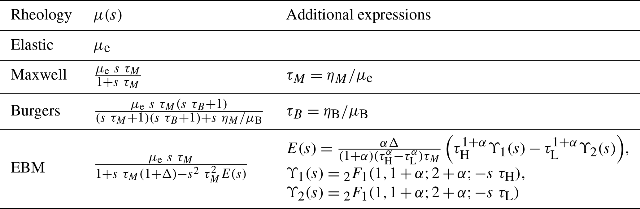
where $\overline{\overline{\mathit{\epsilon }}}$ is the strain tensor obtained from $\overline{\mathit{u}}$ and its spatial derivatives. Table 3 lists the expression of μ(s) for different rheology models, and the bulk modulus κ is assumed to be independent of frequency (Ivins et al., 2022), thus $\mathit{\lambda }\left(s\right)=\mathit{\kappa }-\frac{\mathrm{2}}{\mathrm{3}}\mathit{\mu }\left(s\right)$.

3 Method

Our approach to solving the y_i system closely follows that of Greff-Lefftz and Legros (1997), wherein the solid-Earth model is composed of an elastic lithosphere, a series of viscoelastic mantle layers, an inviscid fluid outer core and a solid inner core. The approach is fundamentally no different than that described by Longman (1962) or Takeuchi and Saito (1972). We number these layers with superscript j=1 to ℒ (the number of layers) from the deepest to the subsurface layer. Each layer is assumed to have a homogenous density ρ, Lamé elastic parameters λ_e and μ_e and any additional rheological parameter such as the Maxwell viscosity η_M, or parameters for the transient rheology (see Table 3).

The system of equations we are looking to solve is a linear equation system consisting of 6(ℒ+1) equations and 6(ℒ+1) unknowns: the y_i variables at each layer interface and for each degree. It is solved once for each spherical harmonic degree n and frequency s by a linear equation solver. In the following subsections we lay out these equations and how to obtain them through boundary conditions at layer boundaries and the propagation of y_i variables within layers.

Table 3 Parameterization of the rheology in the Laplace domain. Note that compressible cases assume $\mathit{\lambda }\left(s\right)=\mathit{\kappa }-\frac{\mathrm{2}}{\mathrm{3}}\mathit{\mu }\left(s\right)$ for all rheologies (Ivins et al., 2022).

3.1 Boundary and continuity conditions

Here we list the equations governing the y_i system at the Earth's center, surface and interfaces between layers.

• At the Earth surface (r=a), ^ℒy₄=0, ^ℒy₁ and ^ℒy₃ are free (free surface hypothesis), and ^ℒy₂, ^ℒy₅, ^ℒy₆ are related to the surface forcing S by the following equations. For n>1 and if the forcing type is surface loading (δ_L=1):

  $$\begin{array}{}\text{(19)}& {\displaystyle }{y}_{\mathrm{2}}\left(a\right)=-{\displaystyle \frac{\mathrm{2}n+\mathrm{1}}{\mathrm{3}}}{\displaystyle \frac{{\mathit{\rho }}_{\mathrm{E}}}{\stackrel{\mathrm{̃}}{\mathit{\mu }}}}{S}_n^m\text{(20)}& {\displaystyle }{y}_{\mathrm{6}}\left(a\right)+{\displaystyle \frac{n+\mathrm{1}}{a}}{y}_{\mathrm{5}}\left(a\right)={\displaystyle \frac{\mathrm{2}n+\mathrm{1}}{g_{s}a}}{S}_n^m\end{array}$$

  with ρ_E the mean Earth density and a the Earth surface radius. For n>1 and if the forcing type is tidal (δ_L=0), there is no radial traction related to the weight of the load, thus:

  $$\begin{array}{}\text{(21)}& {\displaystyle }{y}_{\mathrm{2}}\left(a\right)=\mathrm{0}\text{(22)}& {\displaystyle }{y}_{\mathrm{6}}\left(a\right)+{\displaystyle \frac{n+\mathrm{1}}{a}}{y}_{\mathrm{5}}\left(a\right)={\displaystyle \frac{\mathrm{2}n+\mathrm{1}}{g_{\mathrm{S}}a}}{S}_n^m\end{array}$$

  When n=1, in both cases, the system degenerates and we must impose y₅=0 as an additional boundary condition to fix the center of the frame at the center of mass of the system (including the whole solid-Earth Earth and any surface load). This is because the degree one term of the gravity potential has the unique property to be directly linked to the position of the center of mass in the frame.

  Considering that the Love numbers represent the proportionality coefficients between the forcing S and the resulting deformation, we set $S_n^m=\mathrm{1}$ in the above equations and subsequently in our approach. This yields:

  $$\begin{array}{}\text{(23)}& \left(\begin{array}{cccccc}\mathrm{0}& \mathrm{0}& \mathrm{0}& \mathrm{1}& \mathrm{0}& \mathrm{0}\\ \mathrm{0}& \mathrm{1}& \mathrm{0}& \mathrm{0}& \mathrm{0}& \mathrm{0}\\ \mathrm{0}& \mathrm{0}& \mathrm{0}& \mathrm{0}& \frac{n+\mathrm{1}}{a}& \mathrm{1}\end{array}\right){}^{\mathcal{L}}\overline{\mathbf{y}}\left(a\right)=\left(\begin{array}{c}\mathrm{0}\\ -{\mathit{\delta }}_L\frac{\mathrm{2}n+\mathrm{1}}{\mathrm{3}}\frac{{\mathit{\rho }}_E}{\stackrel{\mathrm{̃}}{\mathit{\mu }}}\\ {\mathit{\delta }}_{\mathrm{1}n}\frac{\mathrm{2}n+\mathrm{1}}{g_{S}a}\end{array}\right)\end{array}$$

• At solid-solid interfaces (between mantle and lithospheric layers), all of y_1..6 variables are continuous, meaning:

  $$\begin{array}{}\text{(24)}& {}^j\overline{\mathbf{y}}\left(r\right)+\left(\begin{array}{cccccc}-\mathrm{1}& \mathrm{0}& \mathrm{0}& \mathrm{0}& \mathrm{0}& \mathrm{0}\\ \mathrm{0}& -\mathrm{1}& \mathrm{0}& \mathrm{0}& \mathrm{0}& \mathrm{0}\\ \mathrm{0}& \mathrm{0}& -\mathrm{1}& \mathrm{0}& \mathrm{0}& \mathrm{0}\\ \mathrm{0}& \mathrm{0}& \mathrm{0}& -\mathrm{1}& \mathrm{0}& \mathrm{0}\\ \mathrm{0}& \mathrm{0}& \mathrm{0}& \mathrm{0}& -\mathrm{1}& \mathrm{0}\\ \mathrm{0}& \mathrm{0}& \mathrm{0}& \mathrm{0}& \mathrm{0}& -\mathrm{1}\end{array}\right){}^{j+\mathrm{1}}\overline{\mathbf{y}}\left(r\right)=\overline{\mathbf{0}}\end{array}$$

• At liquid-solid interfaces, i.e. at the core-mantle and inner-core boundaries (CMB and ICB respectively), we assume that the fluid core's shape follows an equipotential. This ties y₁, y₂ and y₆ together as the radial displacement at the CMB or ICB can be used to calculate directly the excess of pressure and gravity from the other two components. For an in-depth explanation we direct the reader to Greff-Lefftz and Legros (1997). We also know that y₅ is continuous, y₄=0 because the fluid core cannot sustain deviatoric stresses, and y₃ is undermined, effectively decoupling the horizontal motion at both interfaces. For our purposes, this means the system at the ICB is described as the following:

  $$\begin{array}{}\text{(25)}& {}^{\mathrm{2}}\overline{\mathbf{y}}\left(b\right)+\left(\begin{array}{cccccc}-\mathrm{1}& \mathrm{0}& \mathrm{0}& \mathrm{0}& -\frac{\mathrm{1}}{g}& \mathrm{0}\\ -{\mathit{\rho }}^{\mathrm{2}}ga& \mathrm{0}& \mathrm{0}& \mathrm{0}& \mathrm{0}& \mathrm{0}\\ \mathrm{0}& \mathrm{0}& -\mathrm{1}& \mathrm{0}& \mathrm{0}& \mathrm{0}\\ \mathrm{0}& \mathrm{0}& \mathrm{0}& \mathrm{0}& \mathrm{0}& \mathrm{0}\\ \mathrm{0}& \mathrm{0}& \mathrm{0}& \mathrm{0}& -\mathrm{1}& \mathrm{0}\\ \mathit{\gamma }\mathit{\rho }{g}_S& \mathrm{0}& \mathrm{0}& \mathrm{0}& \mathrm{0}& -\mathrm{1}\end{array}\right){}^{\mathrm{3}}\overline{\mathbf{y}}\left(b\right)=\overline{\mathbf{0}}\end{array}$$

  where superscripts 1 and 2 refer to terms in the inner and outer core layers, respectively.

  At the CMB we have:

  $$\begin{array}{}\text{(26)}& {}^{\mathrm{3}}\overline{\mathbf{y}}\left(b\right)+\left(\begin{array}{cccccc}-\mathrm{1}& \mathrm{0}& \mathrm{0}& \mathrm{0}& \frac{{}^{\mathrm{2}}{B}_{\mathrm{55}}}{g}& \frac{{}^{\mathrm{2}}{B}_{\mathrm{56}}}{g}\\ -{\mathit{\rho }}^{\mathrm{2}}ga& \mathrm{0}& \mathrm{0}& \mathrm{0}& \mathrm{0}& \mathrm{0}\\ \mathrm{0}& \mathrm{0}& -\mathrm{1}& \mathrm{0}& \mathrm{0}& \mathrm{0}\\ \mathrm{0}& \mathrm{0}& \mathrm{0}& \mathrm{0}& \mathrm{0}& \mathrm{0}\\ \mathrm{0}& \mathrm{0}& \mathrm{0}& \mathrm{0}& -\mathrm{1}& \mathrm{0}\\ \mathit{\gamma }\mathit{\rho }{g}_S& \mathrm{0}& \mathrm{0}& \mathrm{0}& \mathrm{0}& -\mathrm{1}\end{array}\right){}^{\mathrm{2}}\overline{\mathbf{y}}\left(b\right)=\overline{\mathbf{0}}\end{array}$$

  Note that because y₁ in the outer core is not independent of y₅ and y₆, the boundary conditions at the CMB must use propagation terms ²B₅₅ and ²B₅₆ associated with y₅ and y₆ in order to explicitly connect the 2-variable system in the outer core to the other y_i variables (see Sects. 3.3 and 3.4).

3.2 Analytical propagation of the y_i system from the Earth's center to the innermost interface

We use the incompressible homogenous solid sphere solution (hereafter referred to as the inner sphere solution) from Greff-Lefftz and Legros (1997) to effectively create boundary conditions for $y_{\mathrm{3}},y_{\mathrm{4}},y_{\mathrm{5}}$ at r=r_inner (the other 3 variables must be null within the inner sphere because they follow terms in r⁻ⁿ that would otherwise diverge at r=0). We employ this method because the numerical approach used for the propagation in other layers leads to divergent terms.

We employ this method because the numerical approach used for the propagation in other layers leads to divergent terms. At r=r_inner:

$$\begin{array}{}\text{(27)}& \left(\begin{array}{cccccc}\frac{r}{a}& {\mathcal{A}}_{\mathrm{1}}& \frac{n+\mathrm{3}}{n(n+\mathrm{1})}\frac{r}{a}& \mathrm{2}\frac{\mathit{\mu }}{\stackrel{\mathrm{̃}}{\mathit{\mu }}}\frac{n+\mathrm{2}}{n+\mathrm{1}}& \mathrm{0}& \frac{\mathrm{4}\mathit{\pi }{\mathit{\rho }}_{I}Gr}{g_S}\\ \frac{\mathrm{1}}{ra}& {\mathcal{A}}_{\mathrm{2}}& \frac{\mathrm{1}}{nra}& \mathrm{2}\frac{\mathit{\mu }}{\stackrel{\mathrm{̃}}{\mathit{\mu }}}\frac{n-\mathrm{1}}{n{r}^{\mathrm{2}}}& \mathrm{0}& \frac{\mathrm{4}\mathit{\pi }{\mathit{\rho }}_{I}G}{r{g}_S}\\ \mathrm{0}& -\frac{{\mathit{\rho }}_I}{\stackrel{\mathrm{̃}}{\mathit{\mu }}}& \mathrm{0}& \mathrm{0}& \frac{\mathrm{1}}{g_{S}a}& \frac{n}{g_S}\end{array}\right){}^{\mathrm{1}}\overline{\mathbf{y}}\left(r\right)=\overline{\mathbf{0}},\end{array}$$

with ρ_I is the average density below r_inner, ${\mathcal{A}}_{\mathrm{1}}=\mathrm{2}\frac{\mathit{\mu }}{\stackrel{\mathrm{̃}}{\mathit{\mu }}}(n-\mathrm{1}-\frac{\mathrm{3}}{n})+\frac{\mathrm{4}\mathit{\pi }{\mathit{\rho }}_I^{\mathrm{2}}G}{\mathrm{3}\stackrel{\mathrm{̃}}{\mathit{\mu }}}{r}^{\mathrm{2}}$ and ${\mathcal{A}}_{\mathrm{2}}=\mathrm{2}\frac{\mathit{\mu }}{\stackrel{\mathrm{̃}}{\mathit{\mu }}}\frac{n-\mathrm{1}}{r^{\mathrm{2}}}+\frac{\mathrm{4}\mathit{\pi }{\mathit{\rho }}_I^{\mathrm{2}}G}{\mathrm{3}\stackrel{\mathrm{̃}}{\mathit{\mu }}}$.

3.3 Propagation between the bottom and top interface of each solid layer

In a solid layer, the following relation exists between y_i variables and their radial derivatives (Alterman et al., 1959):

$$\begin{array}{}\text{(28)}& \dot{\overline{\mathbf{y}}}=\overline{\overline{\mathbf{D}}}\overline{\mathbf{y}}\end{array}$$

with the derivative coefficient matrix:

$$\begin{array}{}\text{(29)}& \begin{array}{rl}& \overline{\overline{\mathbf{D}}}=\\ & \left(\begin{array}{cccc}-\frac{\mathrm{2}\mathit{\lambda }}{x(\mathit{\lambda }+\mathrm{2}\mathit{\mu })}& \frac{\stackrel{\mathrm{̃}}{\mathit{\mu }}}{\mathit{\lambda }+\mathrm{2}\mathit{\mu }}& \frac{n(n+\mathrm{1})\mathit{\lambda }}{x(\mathit{\lambda }+\mathrm{2}\mathit{\mu })}& \mathrm{\dots }\\ -\left(\mathrm{4}\mathit{\rho }gax-\frac{\mathrm{12}\mathit{\mu }(\mathit{\lambda }+\frac{\mathrm{2}}{\mathrm{3}}\mathit{\mu })}{\mathit{\lambda }+\mathrm{2}\mathit{\mu }}\right)\frac{\mathrm{1}}{\stackrel{\mathrm{̃}}{\mathit{\mu }}{x}^{\mathrm{2}}}& -\frac{\mathrm{4}\mathit{\mu }}{x(\mathit{\lambda }+\mathrm{2}\mathit{\mu })}& \left(\mathit{\rho }gax-\frac{\mathrm{6}\mathit{\mu }(\mathit{\lambda }+\frac{\mathrm{2}}{\mathrm{3}}\mathit{\mu })}{\mathit{\lambda }+\mathrm{2}\mathit{\mu }}\right)\frac{n(n+\mathrm{1})}{\stackrel{\mathrm{̃}}{\mathit{\mu }}{x}^{\mathrm{2}}}& \mathrm{\dots }\\ -\frac{\mathrm{1}}{x}& \mathrm{0}& \frac{\mathrm{1}}{x}& \mathrm{\dots }\\ \frac{\mathrm{1}}{\stackrel{\mathrm{̃}}{\mathit{\mu }}{x}^{\mathrm{2}}}\left(\mathit{\rho }gax-\frac{\mathrm{6}\mathit{\mu }(\mathit{\lambda }+\frac{\mathrm{2}}{\mathrm{3}}\mathit{\mu })}{\mathit{\lambda }+\mathrm{2}\mathit{\mu }}\right)& -\frac{\mathit{\lambda }}{\mathit{\lambda }+\mathrm{2}\mathit{\mu }}& \frac{\mathit{\mu }}{\stackrel{\mathrm{̃}}{\mathit{\mu }}}\frac{\mathrm{2}\left(\mathrm{2}\mathit{\mu }\left(n(n+\mathrm{1})-\mathrm{1}\right)+\mathit{\lambda }\left(\mathrm{2}n(n+\mathrm{1})-\mathrm{1}\right)\right)}{(\mathit{\lambda }+\mathrm{2}\mathit{\mu })x^{\mathrm{2}}}& \mathrm{\dots }\\ \mathrm{4}\mathit{\pi }\mathit{\rho }G\frac{a}{g_{\mathrm{S}}}& \mathrm{0}& \mathrm{0}& \mathrm{\dots }\\ \mathrm{0}& \mathrm{0}& -\mathrm{4}\mathit{\pi }\mathit{\rho }G\frac{a}{g_{\mathrm{S}}}\frac{n(n+\mathrm{1})}{x}& \mathrm{\dots }\end{array}\right.\\ & \left.\begin{array}{cccc}\mathrm{\dots }& \mathrm{0}& \mathrm{0}& \mathrm{0}\\ \mathrm{\dots }& \frac{n(n+\mathrm{1})}{x}& \mathrm{0}& -\frac{\mathit{\rho }}{\stackrel{\mathrm{̃}}{\mathit{\rho }}}\\ \mathrm{\dots }& \frac{\stackrel{\mathrm{̃}}{\mathit{\mu }}}{\mathit{\mu }}& \mathrm{0}& \mathrm{0}\\ \mathrm{\dots }& -\frac{\mathrm{3}}{x}& -\frac{\mathit{\rho }}{\stackrel{\mathrm{̃}}{\mathit{\rho }}x}& \mathrm{0}\\ \mathrm{\dots }& \mathrm{0}& \mathrm{0}& \mathrm{1}\\ \mathrm{\dots }& \mathrm{0}& \frac{n(n+\mathrm{1})}{x^{\mathrm{2}}}& -\frac{\mathrm{2}}{x}\end{array}\right)\end{array}\end{array}$$

where μ=μ(s) and λ=λ(s) are parameterized via their rheological expressions in Table 3. In this step, we aim to use the above expression to derive the relationship between the y_i values at the bottom and the top of layer j:

$$\begin{array}{}\text{(30)}& {}^j\overline{\mathbf{y}}\left(r_{\mathrm{top}}\right)={}^{\mathbf{j}}\overline{\overline{\mathbf{B}}}{}^j\overline{\mathbf{y}}\left(r_{\mathrm{bottom}}\right)\end{array}$$

Matrix $\overline{\overline{\mathbf{B}}}$ (sometimes referred to as the fundamental or propagation matrix, e.g. Spada et al., 2011) is a 6-by-6 coefficient matrix that can be used to propagate y_i values from r_bottom to r_top within the layer, discretized along a radial grid with step Δr. The propagation matrix is computed numerically via the following method:

1. Let r₁:=r_bottom at the bottom of the layer, q:=1 and $y_{i=q}\left(r_{\mathrm{1}}\right):=\mathrm{1}$ and $y_{i\ne q}\left(r_{\mathrm{1}}\right):=\mathrm{0}$.

2. Let $r_{\mathrm{2}}:=r_{\mathrm{1}}+\mathrm{2}\mathrm{\Delta }r$. Compute y_i(r₂) using y_i(r₁), the analytical expression of y_i derivatives and the Runge-Kutta 4 method. The latter involves evaluating $\overline{\overline{\mathbf{D}}}$ (Eq. 29) at $x=r_{\mathrm{1}}/a$, $x=(r_{\mathrm{1}}+\mathrm{\Delta }r)/a$ and $x=(r_{\mathrm{1}}+\mathrm{2}\mathrm{\Delta }r)/a$ to compute the average slope $<\overline{\overline{\mathbf{D}}}>$ over [r₁, r₂] then $\overline{\mathit{y}}\left(r_{\mathrm{2}}\right)=\overline{\mathit{y}}\left(r_{\mathrm{1}}\right)+\mathrm{2}\mathrm{\Delta }r<\overline{\overline{\mathbf{D}}}>\overline{\mathit{y}}\left(r_{\mathrm{1}}\right)$. Update r₁:=r₂.

3. Repeat step 2 until r₂=r_top at the top of the layer. We then have ^jB_qi:=y_i(r_top).

4. Repeat steps 1–3 for $q\in [\mathrm{2};\mathrm{6}]$.

3.4 Propagation within the fluid core

The outer core material is taken to be an inviscid fluid, therefore the radial traction y₄=0 (no shear stress is supported), and y₃ is undetermined. Under the hypothesis that the shape of the fluid core interfaces is described by gravity equipotential surfaces (Chinnery, 1975; Greff-Lefftz and Legros, 1997), y₁ is no longer independent from y₅ and y₆, and y₂ only reflects the change in lithostatic pressure which can be computed from y₁. As a result, the system is reduced to a 2 independent variable system based on y₅ and y₆ (Eq. 31), as in Greff-Lefftz and Legros (1997). A similar method to the previous section is then employed to propagate y₅ and y₆ through the outer core, the rest of the variables being recovered via boundary conditions laid out in Eqs. (25) and (26).

Within the fluid core, the effective y_i system is therefore:

$$\begin{array}{}\text{(31)}& \left(\begin{array}{c}\dot{{}^{\mathrm{2}}{y}_{\mathrm{5}}}\\ \dot{{}^{\mathrm{2}}{y}_{\mathrm{6}}}\end{array}\right)=\overline{\overline{\mathbf{D}}}\left(\begin{array}{c}{}^{\mathrm{2}}{y}_{\mathrm{5}}\\ {}^{\mathrm{2}}{y}_{\mathrm{6}}\end{array}\right)\end{array}$$

with:

$$\begin{array}{}\text{(32)}& \overline{\overline{\mathbf{D}}}=\left(\begin{array}{cc}\mathrm{4}\mathit{\pi }\mathit{\rho }G\frac{a}{g}& \mathrm{1}\\ \left(-\mathrm{16}\mathit{\pi }\mathit{\rho }G\frac{a}{g}+\frac{n(n+\mathrm{1})}{x}\right)\frac{\mathrm{1}}{x}& -\frac{\mathrm{2}}{x}-\mathrm{4}\mathit{\pi }\mathit{\rho }G\frac{a}{g}\end{array}\right)\end{array}$$

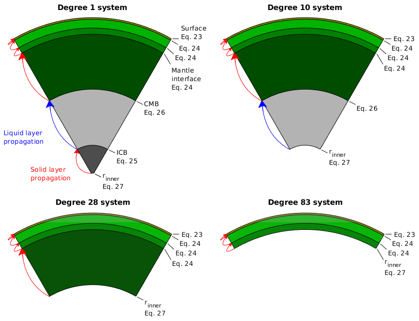
Figure 1 Example of the effective implementation of the y_i system for benchmark Earth model M3-L70-V01 (Spada et al., 2011) and the initial configuration at degree 1, and for the spherical harmonic degrees where the first 3 layers are removed from the system. Applied boundary conditions are indicated by their equation numbers, and colored arrows indicate propagation steps carried out between the bottom and top of each active layer. In each case r_inner corresponds to radius of the interface where Eq. (27) is applied.

3.5 Inverse Laplace transform

In this step we are looking for a method to compute time-dependent Love numbers, h(t), k(t), and l(t) from the estimates of frequency-dependent Love numbers h(s), k(s), and l(s). Our approach here is motivated by our goal to employ Love numbers alongside mass transport models, where the coupled model alternatively computes the change of ice thickness, water column height, ocean pressure, etc., and the ensuing solid-Earth response. In particular, it has to be possible to incrementally compute the ongoing and evolving Earth response before the complete time series of surface mass changes is known. Our choice is to assume that the temporal form of the forcing potential is a unit Heaviside function such that H(t):=1 for t≥0, H(t)=0 for t<0. The forcing potential can then be discretized as follows:

$$\begin{array}{}\text{(33)}& S_n^m\left(t\right)=\sum _{t_{\mathrm{L}}=\mathrm{0}}^t{S}_n^m\left(t_{\mathrm{L}}\right)H(t-t_{\mathrm{L}})\end{array}$$

And thus with Heaviside Love numbers, the temporal convolution in Eq. (17) becomes:

$$\begin{array}{}\text{(34)}& \begin{array}{rl}\left(\begin{array}{c}N(\mathit{\theta },\mathit{\phi },t)\\ u_r(\mathit{\theta },\mathit{\phi },t)\\ u_E(\mathit{\theta },\mathit{\phi },t)\\ u_N(\mathit{\theta },\mathit{\phi },t)\end{array}\right)& =\sum _{t_L=\mathrm{0}}^t\sum _{n,m}{\displaystyle \frac{S_n^m\left(t_L\right)}{g_S}}H(t-t_L)\\ & \times \left(\begin{array}{c}{\mathit{\delta }}^L+k_n(t-t_L)\\ h_n(t-t_L)\\ l_n(t-t_L)\frac{\mathrm{1}}{sin\left(\mathit{\theta }\right)}\frac{\partial }{\partial \mathit{\phi }}\\ -l_n(t-t_L)\frac{\partial }{\partial \mathit{\theta }}\end{array}\right)Y_n^m(\mathit{\theta },\mathit{\phi })\end{array}\end{array}$$

Several methods are available to perform this inverse Laplace transform, and the respective advantages and shortcomings of the main approaches used in GIA are discussed in Spada and Boschi (2006). Here, we choose to employ a method known as the Post-Widder formulation, that has been successfully employed by Spada and Boschi (2006) for Love number computation. This method is a purely numerical approach to computing the inverse Laplace transform, based on the evaluation of successive derivatives of the spectral Love numbers (Abate and Valkó, 2004). It does not require the exploration of the complex frequency plane, nor a priori of the relaxation modes. This makes it the candidate of choice to compute complex rheology structures we are interested in, and in particular non-Maxwellian rheologies such as the Extended Burgers Material. This is because we expect an infinite number of relaxation modes from the distribution governing the transient relaxation, as it corresponds to a continuous distribution of viscosities with associated time scales ranging from τ_L to τ_H (Ivins et al., 2020).

On the other hand, this method is known to have drawbacks for compressible models. Plag and Jüttner (1995); Hanyk et al. (1999); Vermeersen and Mitrovica (2000) identify two types of gravitational instability affecting Maxwell compressible regimes: (1) dilatation modes, which depend on the ratio between Lamé parameters, can most affect low degrees and horizontal deformation; and (2) Rayleigh-Taylor instabilities, related to density stratification, impact models with few mantle layers the most. Using traditional normal mode approaches (Peltier, 1974), one is normally able to identify and exclude unstable modes based on the sign of their relaxation time. This is not possible with the Post-Widder method as individual modes are not identified, and as a result, there is a chance that particular choices of frequency samples lead to numerical artifacts in the results if the system is solved near the frequency of an unstable mode. Mitigation strategies can be employed to reduce both the likelihood of encountering such modes and their amplitude. Vermeersen and Mitrovica (2000) indicates that the input model for radial density and elastic parameter profiles (such as PREM,  Dziewonski and Anderson, 1981) may be checked to detect instabilities in the initial state and emphasizes the stabilizing role of an elastic lithosphere; Hanyk et al. (1999) note that finer layering of the Earth model increases the timescales of the instable modes, such that their contributions may be lessened at or below post-glacial deformation time scales.

The Post-Widder formulation is implemented as follows:

$$\begin{array}{}\text{(35)}& f(t{)}_M=\sum _{p=\mathrm{1}}^{\mathrm{2}M}{\mathit{\xi }}_M^{p}f(s_p),\end{array}$$

where f is the function we wish to perform the inverse Laplace transform of any of the Love numbers, M indicates the maximum number of derivations of f considered, and the frequency samples necessary to estimate f at time t are given by $s_p=\frac{p\ln \left(\mathrm{2}\right)}{t}$. ${\mathit{\xi }}_M^p$ are the coefficients for the frequency samples to get the proper derivatives:

$$\begin{array}{}\text{(36)}& {\mathit{\xi }}_M^p={\displaystyle \frac{(-\mathrm{1}{)}^{p+M}}{p}}\sum _{q=\mathrm{Floor}\left(\frac{p+\mathrm{1}}{\mathrm{2}}\right)}^{min(p,M)}{\displaystyle \frac{q^{M+\mathrm{1}}}{M\mathrm{!}}}{C}_q^M{C}_q^{\mathrm{2}q}{C}_{p-q}^q,\end{array}$$

with $C_p^q$ the binomial coefficient. This method is based on the Saltzer summation for inverse Laplace transform, through Eqs. (2), (6), (7) in Valkó and Abate (2004), and is similar to the accelerated Gaver sequence employed by Spada and Boschi (2006).

The main downside of this approach is its numerical stability, as repeated derivatives of estimated Love numbers is prone to the propagation of errors via catastrophic cancellation. Spada and Boschi (2006) point out that multiprecision environments, supporting up to 128 digits variables, can be helpful in mitigating this effect for larger values of M. Our implementation can be run with either double (16 digits) or quadruple (32 digits) precision. However, we find that the level of systematic errors associated with our method in the propagation step does not allow quadruple precision to improve the accuracy of our solutions with respect to the benchmark solutions. We also found that catastrophic cancellation was more susceptible to happen in near-elastic or near-fluid regimes where the frequency dependence is small. We have found that the ideal value of M is not the same for different values of t. Our approach is thus as follows. If $M_{max}<\mathrm{4}$, we compute $f(t{)}_{M_{max}}$ straightforwardly from Eq. (35), as there are not enough iterations of M to apply our error growth detection method. Otherwise, for each value of t:

1. Compute f(t)₁, f(t)₂, f(t)₃ and f(t)₄. Assume M=4.

2. If $\left|f\right(t{)}_M-f\left(t{)}_{M-\mathrm{1}}\right|>\left|f\right(t{)}_{M-\mathrm{1}}-f\left(t{)}_{M-\mathrm{2}}\right|$ and $\left|f\right(t{)}_{M-\mathrm{1}}-f\left(t{)}_{M-\mathrm{2}}\right|>\left|f\right(t{)}_{M-\mathrm{2}}-f\left(t{)}_{M-\mathrm{3}}\right|$, then the series is labeled as divergent and we choose f(t)_M−2 as the final stable value. The reason why we look for 3 consecutive iterations diverging and not merely 2 is to allow for inflection points in the convergence of the series.

3. Else, increment M by one and compute f(t)_M.

4. Repeat 2 and 3 until either the series diverges or the series reaches the maximum number of iteration M_max.

3.6 Polar motion transfer function

The polar motion transfer function (hereafter PMTF) ℳ is the analog of Love numbers for the movement of the Earth spin axis. This displacement occurs in response to the same forcing and produces additional changes to the Earth gravity potential and bedrock motion known as the rotational feedback (Mitrovica et al., 2005). Here we consider only the secular polar motion, neglecting the Chandler wobble as it produces no long-term trend. Following Spada et al. (2011) we have:

$$\begin{array}{}\text{(37)}& \mathcal{M}\left(s\right)={\displaystyle \frac{\mathrm{1}+k_{\mathrm{2}}\left(s\right)}{\mathrm{1}-k_{\mathrm{2}}^T\left(s\right)/k_{\mathrm{s}}}}.\end{array}$$

with k₂ the degree 2 loading Love number, $k_{\mathrm{2}}^T$ the degree 2 tidal Love number, k_s the secular degree 2 tidal Love number. This function can then be expressed in the time domain as a Heaviside response ℳ(t) via an inverse Laplace transform, by the same process highlighted above for Love numbers. In Fig. 2 we compare the results from our computation with respect to the benchmark of Spada et al. (2011). We find satisfactory agreement with relative errors within 10⁻⁵ for t<100 000 years (which is usually the maximum scale employed in GIA modeling). Therefore, in subsequent comparisons to the benchmark result we focus on reporting the relative error rather than the direct output in our figures, as differences in the left panel are not visible.

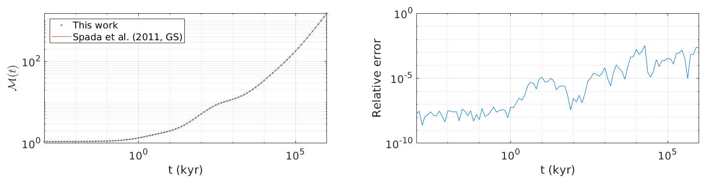
Figure 2 Polar motion transfer function (Heaviside response) for model M3-L70-V01. Left: comparison of absolute values, and right: relative difference between our computation and the reference benchmark from Spada et al. (2011). The benchmark response was computed using normal modes provided by contributor GS in test T-4 in Spada et al. (2011), and Eqs. (23)–(28) therein. Our computation is parameterized with N_grid=6000, $M_{max}=\mathrm{7}$.

4 Structure of the Love number solver

Here we present an overview of the main steps followed by our Love number solver. Figure S2 displays a flowchart summary of this structure for a typical resolution of surface loading Love numbers, while Fig. S3 provides the details of steps taken to solve the y_i system at any given degree n and frequency s. Note that our solver optimizes computation time by identifying a spherical harmonic degree at and above which the deformation is practically contained within the elastic lithosphere, and the viscous component of the deformation can be neglected. More information about the threshold n_vmax and the comparison between elastic and pseudo-fluid Love numbers is provided in Sect. 5.1.3.

1. Initialization: Gather parameters from ISSM wrapper. Compute g₀(r), and λ(s), μ(s) for each layer.

2. Compute elastic Love numbers $h_{n,\mathrm{e}},k_{n,\mathrm{e}},l_{n,\mathrm{e}}$ and pseudo-fluid Love numbers $h_{n,\mathrm{f}},k_{n,\mathrm{f}},l_{n,\mathrm{f}}$ for $n\in [n_{min},n_{max}]$.

3. Determine degree n_vmax where the viscous part of Love numbers becomes negligible.

4. Distribute the frequency vector between CPU nodes for parallel computation.

5. For each node, compute $h_n\left(s\right),k_n\left(s\right),l_n\left(s\right)$ for $n\in [n_{min},n_{\mathrm{vmax}}]$ for its assigned list of frequencies. For $n\ge n_{\mathrm{vmax}}+\mathrm{1}$ the Love numbers are set for all values of s to the elastic values from step 2.

6. If the forcing type is set to surface loading, also compute degree 2 tidal Love numbers $h_{\mathrm{2}}^T\left(s\right),k_{\mathrm{2}}^T\left(s\right),l_{\mathrm{2}}^T\left(s\right)$ for the polar motion transfer function (PMTF) and rotational feedback response.

7. Perform the inverse Laplace transform of $h_n\left(s\right),k_n\left(s\right),l_n\left(s\right)$ to get the Heaviside Love numbers $h_n\left(t\right),k_n\left(t\right),l_n\left(t\right)$. The Laplace transform of tidal degree 2 Love numbers and PMTF is also performed if they were computed in the previous step.

8. Assemble Love numbers and PMTF across CPU nodes from parallel computation.

9. Output Love numbers and PMTF.

5 Performance

In this section we report metrics related to (1) the accuracy of our results relative to benchmark tests from Spada et al. (2011, hereafter S11), specifically the computations from TABOO as this entry was available for all tests, (2) the stability and available approximations for the computation at high spherical harmonic degree, and (3) computation time under different optimization schemes and parallel settings. The benchmark results only features incompressible Earth models, which we approximate by imposing ^jλ_e=10²⁰ Pa throughout the Earth model. Our reference is Test-5/1 for time-domain Love numbers for both Earth models therein, containing results for a maximum degree of n=256. Two main Earth structures are employed: model M3-L70-V01 is structured with a low number of layers (1 elastic lithosphere layer, 3 viscoelastic mantle layers) that are thinner as the radius gets closer to the Earth surface; model VSS96 consists of a total of 29 mantle and lithosphere layers of similar thickness. To both of these Earth models we add 2 layers for the liquid outer core and inner core that are inviscid and match the density specified in Spada et al. (2011). For the purpose of examining the elastic and fluid behavior of our solver at high degree, we also use a 500-layers Earth model based on the Preliminary Reference Earth Model (PREM-500,  Dziewonski and Anderson, 1981) with a viscosity of 10²¹ Pa s throughout the mantle and variable lithospheric thickness. Our tests were performed with a 20-core Intel Xeon(R) E5-2687W v3 CPU operating at 3.10 GHz, on a 64-bit RedHat operating system.

5.1 Optimization

5.1.1 Coefficients of y_i matrix in the propagation

Our main strategy to reduce computation time of the Love number system is to minimize the number of redundant recomputations of terms in the y_i coefficient matrix in the propagation step. To this end it is useful to recognize the basic structure of the computation as 4 nested loops, spanning, in the following order, (1) the spherical harmonic degrees; (2) frequencies; (3) the 6 y_i variables in the propagation step and (4) the radial grid. Our goal here is to avoid recomputing terms that do not change in lower loop levels. Instead we precompute terms for the coefficient matrix before loops 1, 2 and 4 in subsequent loops. No such optimization can be done for loop 3 as terms are not recurrent between variables.

We first start by defining the following factors:

$$\begin{array}{}\text{(38)}& \begin{array}{ll}\stackrel{\mathrm{̃}}{\mathit{\rho }}=\frac{\stackrel{\mathrm{̃}}{\mathit{\mu }}}{g_{\mathrm{S}}a},& \underset{\mathrm{¯}}{\underset{\mathrm{¯}}{\mathit{\kappa }}}=\underset{\mathrm{¯}}{\underset{\mathrm{¯}}{\mathit{\lambda }}}+\frac{\mathrm{2}}{\mathrm{3}}\underset{\mathrm{¯}}{\underset{\mathrm{¯}}{\mathit{\mu }}},\\ \underset{\mathrm{¯}}{\underset{\mathrm{¯}}{\mathit{\beta }}}=\underset{\mathrm{¯}}{\underset{\mathrm{¯}}{\mathit{\lambda }}}+\mathrm{2}\underset{\mathrm{¯}}{\underset{\mathrm{¯}}{\mathit{\mu }}},& \mathit{\gamma }=\mathrm{4}\mathit{\pi }\mathit{\rho }G\frac{a}{g_{\mathrm{S}}},\\ \underset{\mathrm{¯}}{L}=\underset{\mathrm{¯}}{n}(\underset{\mathrm{¯}}{n}+\mathrm{1})& \\ \underset{\mathrm{¯}}{\underset{\mathrm{¯}}{{\mathit{\kappa }}^{\prime }}}=\mathrm{3}\mathit{\kappa }/\underset{\mathrm{¯}}{\underset{\mathrm{¯}}{\mathit{\beta }}},& \underset{\mathrm{¯}}{\underset{\mathrm{¯}}{{\mathit{\mu }}^{\prime }}}=\underset{\mathrm{¯}}{\underset{\mathrm{¯}}{\mathit{\mu }}}/\stackrel{\mathrm{̃}}{\mathit{\mu }},\\ {\mathit{\sigma }}^{\prime }=\mathit{\rho }a/\stackrel{\mathrm{̃}}{\mathit{\mu }},& {\mathit{\rho }}^{\prime }=\mathit{\rho }/\stackrel{\mathrm{̃}}{\mathit{\rho }}\\ \underset{\mathrm{¯}}{\underset{\mathrm{¯}}{f_{\mathrm{0}}}}=-\mathrm{2}\underset{\mathrm{¯}}{\underset{\mathrm{¯}}{\mathit{\lambda }/\mathit{\beta }}},& \underset{\mathrm{¯}}{\underset{\mathrm{¯}}{f_{\mathrm{1}}}}=\stackrel{\mathrm{̃}}{\mathit{\mu }}/\underset{\mathrm{¯}}{\underset{\mathrm{¯}}{\mathit{\beta }}},\\ \underset{\mathrm{¯}}{\underset{\mathrm{¯}}{f_{\mathrm{2}}}}=\underset{\mathrm{¯}}{\underset{\mathrm{¯}}{\mathit{\lambda }}}\underset{\mathrm{¯}}{L}/\underset{\mathrm{¯}}{\underset{\mathrm{¯}}{\mathit{\beta }}},& \underset{\mathrm{¯}}{\underset{\mathrm{¯}}{f_{\mathrm{3}}}}=\underset{\mathrm{¯}}{\underset{\mathrm{¯}}{{\mathit{\mu }}^{\prime }{\mathit{\kappa }}^{\prime }}},\\ \underset{\mathrm{¯}}{\underset{\mathrm{¯}}{f_{\mathrm{4}}}}=-\mathrm{4}\underset{\mathrm{¯}}{\underset{\mathrm{¯}}{\mathit{\mu }/\mathit{\beta }}},& \underset{\mathrm{¯}}{f_{\mathrm{5}}}=\underset{\mathrm{¯}}{L}{\mathit{\rho }}^{\prime },\\ \underset{\mathrm{¯}}{\underset{\mathrm{¯}}{f_{\mathrm{6}}}}=-\mathrm{2}\underset{\mathrm{¯}}{\underset{\mathrm{¯}}{{\mathit{\mu }}^{\prime }{\mathit{\kappa }}^{\prime }}}\underset{\mathrm{¯}}{L},& \underset{\mathrm{¯}}{\underset{\mathrm{¯}}{f_{\mathrm{7}}}}=\mathrm{1}/\underset{\mathrm{¯}}{\underset{\mathrm{¯}}{{\mathit{\mu }}^{\prime }}},\\ \underset{\mathrm{¯}}{\underset{\mathrm{¯}}{f_{\mathrm{8}}}}=-\mathrm{2}\underset{\mathrm{¯}}{\underset{\mathrm{¯}}{{\mathit{\mu }}^{\prime }{\mathit{\kappa }}^{\prime }}},& \underset{\mathrm{¯}}{\underset{\mathrm{¯}}{f_{\mathrm{9}}}}=-\underset{\mathrm{¯}}{\underset{\mathrm{¯}}{\mathit{\lambda }/\mathit{\beta }}},\\ \underset{\mathrm{¯}}{\underset{\mathrm{¯}}{f_{\mathrm{10}}}}=\frac{\mathrm{2}\underset{\mathrm{¯}}{\underset{\mathrm{¯}}{{\mathit{\mu }}^{\prime }}}}{\underset{\mathrm{¯}}{\underset{\mathrm{¯}}{\mathit{\beta }}}}\left((\underset{\mathrm{¯}}{\underset{\mathrm{¯}}{\mathit{\lambda }}}+\mathrm{2}\underset{\mathrm{¯}}{\underset{\mathrm{¯}}{\mathit{\mu }}})(\underset{\mathrm{¯}}{L}-\mathrm{1})+\underset{\mathrm{¯}}{\underset{\mathrm{¯}}{\mathit{\lambda }}}\underset{\mathrm{¯}}{L}\right),& \underset{\mathrm{¯}}{f_{\mathrm{11}}}=\mathit{\gamma }\underset{\mathrm{¯}}{L}\end{array}\end{array}$$

Here, f_1.. refer to the precomputed terms in order in which the appear in Eq. (39), terms with a prime symbol ^′ are used for non-dimensionalized quantities (e.g. μ^′ is the non-dimensionalized shear modulus) while terms with a tilde ∼ are used for other scaling constants. Note that underline marking indicates when we precompute terms: terms with no underline are neither frequency-dependent or degree-dependent and are computed only once, before the start of loop 1; terms with single underline are only degree-dependent and are computed once per degree, before loop 2 (i.e. recomputed once per degree); and terms with double underline are frequency-dependent and are computed once per degree and frequency, before loop 3.

Within loops 3 and 4 these factors are used in the propagation of the y_i system as described below. Note that we need to separate the terms that depend on different powers of the non-dimensionalized radius x, as well as the gravity g₀, as these terms change within loop 4.

In its optimal form, Eq. (29) becomes:

$$\begin{array}{}\text{(39)}& \begin{array}{rl}& \overline{\overline{\mathbf{D}}}=\\ & \left(\begin{array}{cccccc}\frac{f_{\mathrm{0}}}{x}& f_{\mathrm{1}}& \frac{f_{\mathrm{2}}}{x}& \mathrm{0}& \mathrm{0}& \mathrm{0}\\ \frac{\mathrm{4}}{x}\left(-{\mathit{\sigma }}^{\prime }{g}_{\mathrm{0}}+\frac{f_{\mathrm{3}}}{x}\right)& \frac{f_{\mathrm{4}}}{x}& \left(f_{\mathrm{5}}{g}_{\mathrm{0}}+\frac{f_{\mathrm{6}}}{x}\right)\frac{\mathrm{1}}{x}& \frac{L}{x}& \mathrm{0}& -{\mathit{\rho }}^{\prime }\\ -\frac{\mathrm{1}}{x}& \mathrm{0}& \frac{\mathrm{1}}{x}& f_{\mathrm{7}}& \mathrm{0}& \mathrm{0}\\ \frac{\mathrm{1}}{x}\left({\mathit{\sigma }}^{\prime }{g}_{\mathrm{0}}+\frac{f_{\mathrm{8}}}{x}\right)& f_{\mathrm{9}}& \frac{f_{\mathrm{10}}}{x^{\mathrm{2}}}& -\frac{\mathrm{3}}{x}& -\frac{{\mathit{\rho }}^{\prime }}{x}& \mathrm{0}\\ \mathit{\gamma }& \mathrm{0}& \mathrm{0}& \mathrm{0}& \mathrm{0}& \mathrm{1}\\ \mathrm{0}& \mathrm{0}& -\frac{f_{\mathrm{11}}}{x}& \mathrm{0}& \frac{L}{x^{\mathrm{2}}}& -\frac{\mathrm{2}}{x}\end{array}\right)\end{array}\end{array}$$

The efficiency improvement to computation time is reported in Table 4. We found that with our method the most computationally expensive step of the Love number solver was by far the propagation of the y_i system within Earth layers. Pre-computing all coefficients before loop 3 (referred to as “prefactoring only” in Table 4) allows for about a 75 % reduction in the computational time compared to the naive implementation. Further decrease of redundant operations can be achieved by pre-computing different terms at different time following colors indicated in Eq. (38) (see entries under “Fully optimized”), cutting the prefactoring time by a factor 3. This amounts to a further 27 % decrease in overall computational time (81 % compared to the naive implementation).

Table 4 Computation time (seconds) for 3 levels of optimization of the y_i system propagation within layers, for model M3-L70-V01 with N_grid=6000, n_CPU=20, $M_{max}=\mathrm{7}$, $n_{max}=\mathrm{800}$ and N_t=100. Here naive implementation refers to computing Eq. (29) each time the propagation step is performed. Prefactoring only refers to computing Eq. (38) each time loop 3 is performed, and using Eq. (39) during the propagation step. Fully optimized computes terms in Eq. (38) before loops 1, 2 or 3 depending on their degree and frequency dependence, and using Eq. (39) in the propagation step. Values are reported with a precision of 0.01 s, and ϵ indicates computation time below this precision threshold.

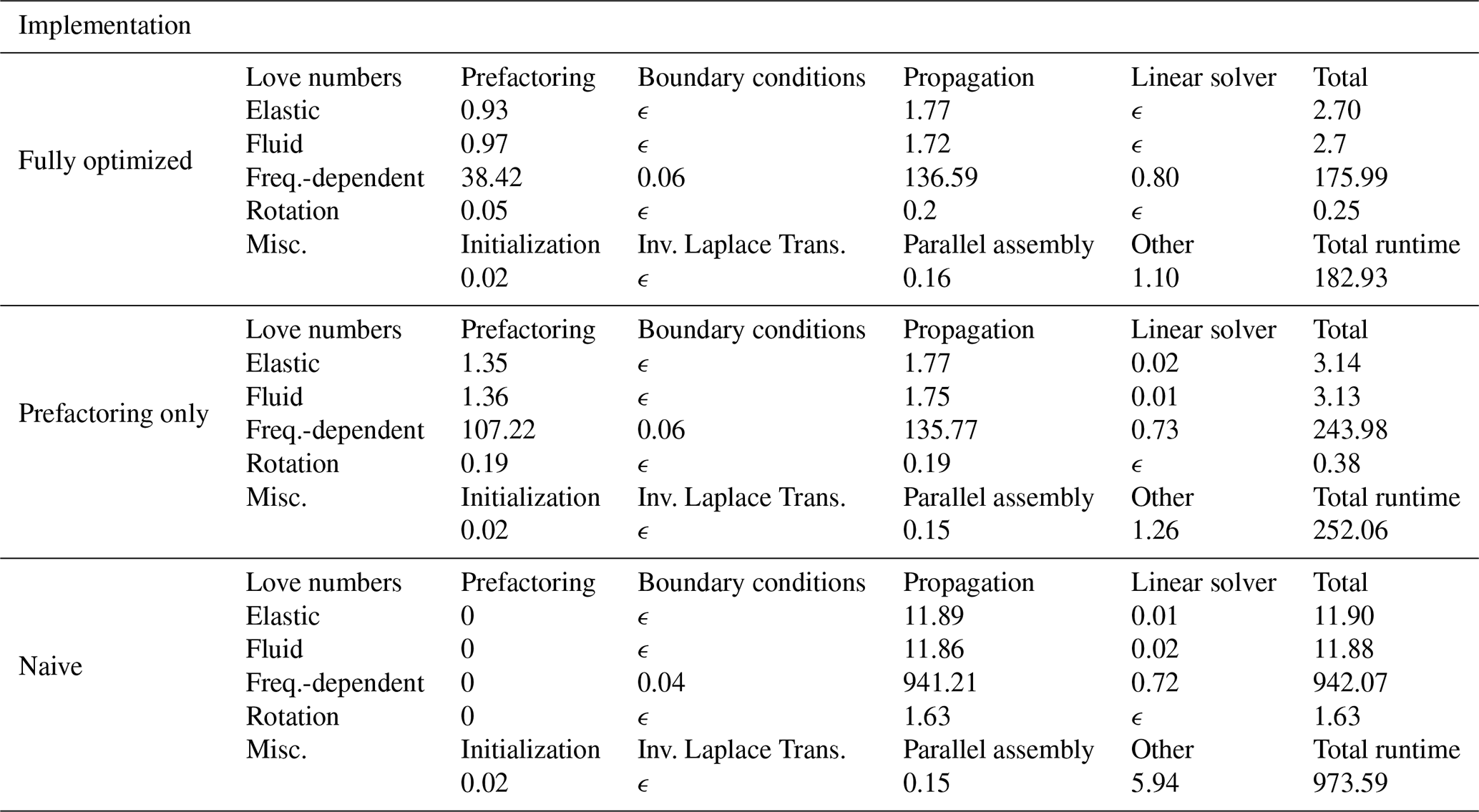
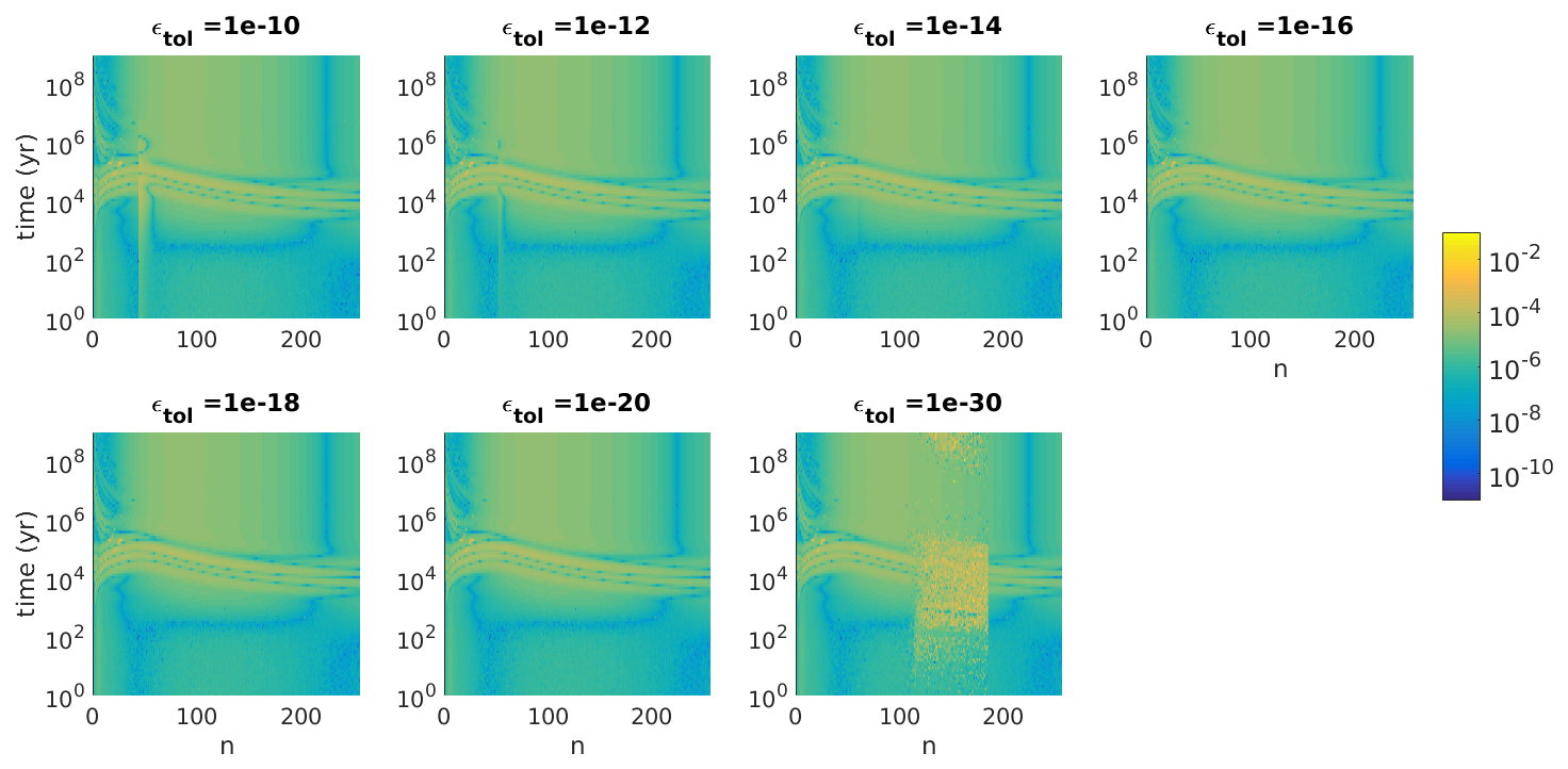
Figure 3 Relative error (colorbar) with respect to the S11 benchmark on time-domain loading Love number h. Each frame represents the error for different value of the threshold ϵ_tol for the deep-to-surface Love numbers ratio.

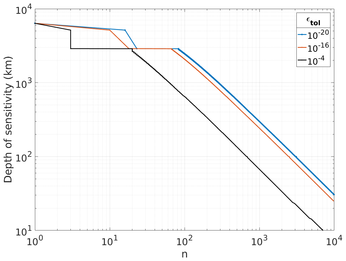
Figure 4 Migration of depth r_inner for the first interface in the resolution of the elastic system. Below this depth, the ratio of deep to surface Love numbers (for all 3 of h, k, l) is less than ϵ_tol.

5.1.2 High-degree computation

As the spherical harmonic degree increases, deformation from surface loading decays increasingly faster with depth. This effect can be physically understood as destructive interference between the peaks and troughs of the surface load potential, which becomes significant at depth greater than the spherical harmonic wavelength. For the y_i system, this means that the conditioning of the equation coefficient matrix gradually degrades as degree increases, until our linear equation solver is no longer able to invert the matrix. In our implementation and for model M3-L70-V01, this happens around degree 243. To get around this limitation and compute high-degree Love numbers, our strategy relies on monitoring the ratio of deformation at the surface and at our innermost interface located at r_inner after the system has been solved at a given degree. At this depth, analogs of Love numbers can be expressed as:

$$\begin{array}{}\text{(40)}& {\displaystyle }{h}_D=y_{\mathrm{1}}\left(r_{\mathrm{inner}}\right)g_{\mathrm{S}}a,\text{(41)}& {\displaystyle }{l}_D=y_{\mathrm{3}}\left(r_{\mathrm{inner}}\right)g_{\mathrm{S}}a,\text{(42)}& {\displaystyle }{k}_D=y_{\mathrm{5}}\left(r_{\mathrm{inner}}\right)g_{\mathrm{S}}a-{\left({\displaystyle \frac{r_{\mathrm{inner}}}{a}}\right)}^n,\end{array}$$

and similarly, surface Love numbers are given by:

$$\begin{array}{}\text{(43)}& {\displaystyle }{h}_S=y_{\mathrm{1}}\left(a\right)g_{\mathrm{S}}a,\text{(44)}& {\displaystyle }{l}_S=y_{\mathrm{3}}\left(a\right)g_{\mathrm{S}}a,\text{(45)}& {\displaystyle }{k}_S=y_{\mathrm{5}}\left(a\right)g_{\mathrm{S}}a-\mathrm{1.0}\end{array}$$

If $min\left\{\left|\frac{h_D}{h_S}\right|,\left|\frac{k_D}{k_S}\right|,\left|\frac{l_D}{l_S}\right|\right\}<{\mathit{ϵ}}_{\mathrm{tol}}$, an arbitrary threshold, we flag the innermost layer to be removed from the y_i system when it is subsequently solved at higher degree. In doing so the 6 equations and unknowns relating to the interface at the bottom of this layer are removed. At the top of this layer, the continuity equations are replaced with the inner sphere solution, which guarantees numerical stability at r=0. In Fig. 3, a performance test against the S11 benchmark is performed with model M3-L70-V01 for several values of ϵ_tol. Choosing either ${\mathit{ϵ}}_{\mathrm{tol}}:={\mathrm{10}}^{-\mathrm{10}}$ or ${\mathit{ϵ}}_{\mathrm{tol}}:={\mathrm{10}}^{-\mathrm{30}}$ reveals additional error from either removing layers too soon or too late, respectively, in the former case because the physics are poorly approximated and the latter case because of the propagation of numerical noise. These results indicate that ${\mathrm{10}}^{-\mathrm{14}}\le {\mathit{ϵ}}_{\mathrm{tol}}\le {\mathrm{10}}^{-\mathrm{20}}$ produce equally accurate solutions, though further testing different Earth model may narrow down this preferred interval. Frames with ${\mathrm{10}}^{-\mathrm{14}}\le {\mathit{ϵ}}_{\mathrm{tol}}\le {\mathrm{10}}^{-\mathrm{20}}$ also serve as a representative example for the distribution of errors (relative to S11) across time and the spherical harmonic degrees. In Fig. 4 we show the depth-degree relationship for the removal of layers for 3 values of ϵ_tol. This is performed for the highly layered PREM-500 model in order to finely detail the migration of the depth sensitivity with the harmonic degree. After r_inner increases past the CMB, we can see a quasi-linear curve for all values of ϵ_tol, indicative of a power-law relationship. The blue and orange curves are both from our recommended interval, and indicate the depth that is numerically relevant to solve the y_i system for any particular degree. This does not mean that the displacement and potential changes are physically large at this depth, and by contrast the black curve indicates where the ratio of depth-to-surface Love numbers reaches less than 0.1 %.

5.1.3 Limits of the sensitivity to viscosity

Another consequence of the Love number depth-dependence described above is that there is a spherical harmonic degree n_vmax above which the deformation is practically contained within the elastic lithosphere. Note that for models with a homogeneous lithosphere this also coincides with the limit where Love numbers tend to their asymptotic value, but these two limits may need to be distinguished for models with several subsurface elastic layers (for example, models detailing the structure of the lithospheric mantle and crust). We also remark that this limit is in theory independent of the viscosity profile or the rheology model chosen to represent viscoelasticity, as it relies on fluid Love numbers. In practice, we expect that very weak sensitivity may arise from imperfect approximation of fluid Love numbers.

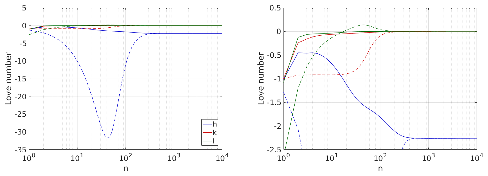
Figure 5 Elastic (solid lines) and pseudo-fluid (dashed lines) Love numbers for the M3-L70-V01 model. The right frame shows a zoomed-in version of the left frame to better highlight the convergence between all elastic and pseudo-fluid Love numbers. For this model, we find that all 3 fluid Love number fall within 0.1 % of their elastic value at degree 875 with $\left|\frac{h_{\mathrm{f}}-h_{\mathrm{e}}}{h_{\mathrm{e}}}\right|=\mathrm{1.89912}\times {\mathrm{10}}^{-\mathrm{6}};\left|\frac{k_{\mathrm{f}}-k_{\mathrm{e}}}{k_{\mathrm{e}}}\right|=\mathrm{1.90551}\times {\mathrm{10}}^{-\mathrm{6}};\left|\frac{l_{\mathrm{f}}-l_{\mathrm{e}}}{l_{\mathrm{e}}}\right|=\mathrm{0.999277}\times {\mathrm{10}}^{-\mathrm{3}}$, with $h_{\mathrm{e}},k_{\mathrm{e}},l_{\mathrm{e}}$ and $h_{\mathrm{f}},k_{\mathrm{f}},l_{\mathrm{f}}$ the elastic and pseudo-fluid Love numbers, respectively.

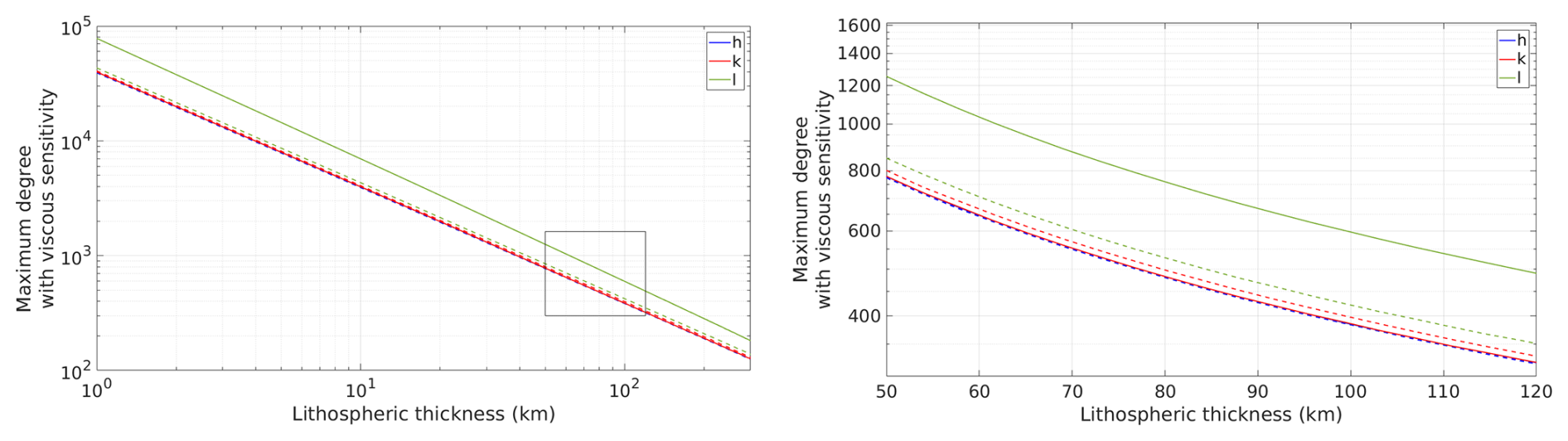
Figure 6 Maximum degree n_vmax where loading Love numbers exhibit frequency sensitivity (i.e. the fluid to elastic difference exceeds 0.1 % of the elastic values), as a function of the lithospheric thickness. Solid lines: incompressible case, dashed lines: compressible case. These curves assume the PREM structure and are insensitive to the viscosity profile. Left: Logarithmic view for a lithospheric thickness between 1 and 300 km; right: linear x-axis view for commonly assumed values of the lithospheric thickness. The bounding box on the left frame shows the location of the right frame axes. Note that the blue line for h is often obscured by the red line for k as both yield similar values of n_vmax.

Detecting this limit is helpful for optimization purposes as the frequency-dependence of Love numbers becomes negligible after this threshold, and so the elastic value becomes sufficient to describe the Earth's response. Our approach to determine the limit n_vmax is to compute “pseudo-fluid” Love numbers using the lowest frequency requested by the user, and the elastic Love numbers before solving the system at any other frequencies. An arbitrary threshold applied to the relative difference between pseudo-fluid and elastic values may be used to determine when the frequency dependence of the system can be neglected for all 3 Love numbers. We find that l is the Love number that exhibits the most sensitivity to viscosity, particularly in the incompressible case, and setting this threshold to 10⁻³ usually results in n_vmax such that h and k are within a relative difference of 10⁻⁵ of their elastic value. Figure 5 illustrates this behavior for model M3-L70-V01 by comparing the elastic Love numbers with their pseudo-fluid counterpart (in this case, the response after t=10⁶ years, following Spada et al., 2011). Figure 6 shows how n_vmax varies with the lithospheric thickness for each of the 3 Love numbers. The results consistently point to a power-law relationship, the threshold being significantly more constraining for the case of l in an incompressible Earth model.

5.2 Accuracy and efficiency

Here we assess the accuracy and computational efficiency of our solver based on the benchmark results of Spada et al. (2011). We then perform 3 different experiments to investigate the performance of our solver. In experiment 1 and 2, we vary the size of the radial grid used for the propagation step (Sect. 3.3), where we compute matrix $\overline{\overline{B}}$ every Δr. Subdividing the layers in this way creates a 1D grid from r_inner to the surface. The questions investigated in comparing experiments 1 and 2 are as follows: (1) for a given number of grid points (a priori equivalent computational resources), are Δr better distributed uniformly across all layers, or should each layer have the same number of propagation steps? (2) what is the ideal total number of grid points N_grid, in order to solve Love numbers accurately, before yielding diminishing returns?

In experiment 1, the number of radial steps is the same in each layer. Therefore thinner layers therein are resolved with a smaller grid resolution Δr. In experiment 2, the grid resolution Δr is the same in all layers, therefore thinner layers therein are discretized with fewer grid points. In experiment 3, we vary the maximum number of iterations within the inverse Laplace Transform.

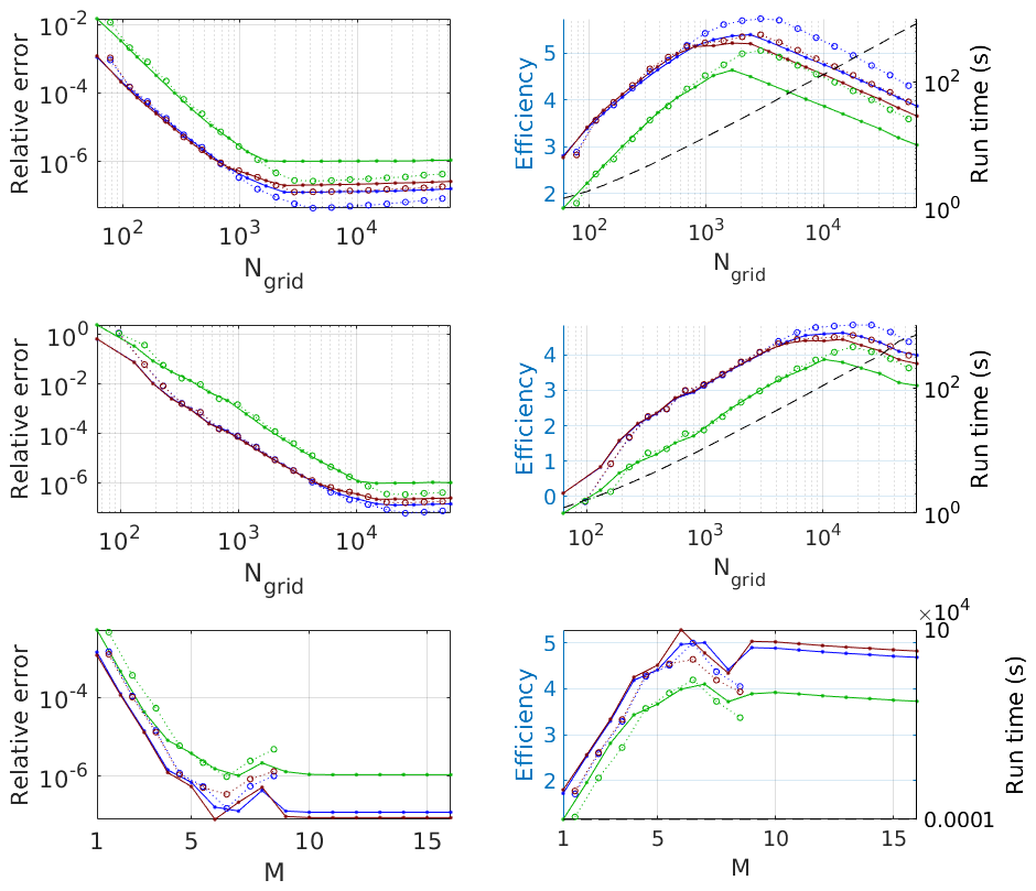
Figure 7 Accuracy of the Love number solver. Left column: Relative error (median value across degrees and frequency) on Heaviside loading Love numbers for model M3-L70-V01 for (h), (k) and (l) (blue, red and green colors respectively). Solid lines: error relative to S11 GS, for external validation purposes. Dotted lines: difference between computations using increasing values (circles) of N_grid or M, for the evaluation of internal convergence. Right column: computational efficiency (−log ₁₀ (median relative error × Run time), colored lines, left y-axis); run time (black dashed line, right y-axis). Top row: increasing the radial grid resolution, with the same number of grid points in each layer. Middle row: increasing the radial grid resolution, keeping the resolution Δr the same for all layers. Bottom row: maximum number of iterations for the Post-Widder inverse Laplace transform. No dotted line is represented for M≥9 as for these cases the median error is 0.

Figure 8 Same as Fig. 7, but for model VSS96.

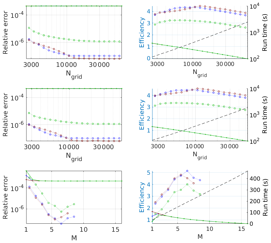
Figure 7 shows that for model M3-L70-V01 it is more efficient to distribute the same number of radial grid points to each layer (experiment 1) than a homogeneous grid size across the whole mantle (experiment 2), with a maximum efficiency reached around $\mathrm{2}\times {\mathrm{10}}^{\mathrm{3}}<N_{\mathrm{grid}}<\mathrm{4}\times {\mathrm{10}}^{\mathrm{3}}$ (with diminishing returns at larger grid sizes) instead of $\mathrm{1}\times {\mathrm{10}}^{\mathrm{4}}<N_{\mathrm{grid}}<\mathrm{3}\times {\mathrm{10}}^{\mathrm{4}}$. In this Earth model, the layer thickness also increases with depth so it is possible that the ideal distribution of grid points be actually one where the radial resolution improves closer to the surface. Figure 8 shows that for model VSS96 in which layers have similar thickness, both approaches are roughly equivalent. The convergence of the Post-Widder algorithm is highlighted in experiment 3 (last row in Figs. 7 and 8). For model M3-L70-V01 we can see that past M=7 the solutions no longer improve with respect to the S11 benchmark, and in fact the internal convergence metric (dotted lines) highlights growing divergence for two iterations before the series is stopped by our error detection algorithm. This is close to the maximum that might be expected a priori for double-precision variables (16 digits): at M=8 we have performed 16 derivatives of our function in the Laplace domain and correspondingly magnified errors through catastrophic cancellation. For model VSS96, our model agreement to the benchmark results appears to be poorer (with residuals on the order of 10⁻⁴–10⁻³) although a similar level of internal convergence to model M3-L70-V01 is achieved for N_grid≈10⁴ and M=7. A comparison between the two benchmark solutions submitted to this test (GS and VK) yields relative differences of the same order of magnitude. It is therefore not clear whether this result indicates that our numerical approach to the propagation of the y_i system accumulates larger errors for highly stratified Earth models, or simply highlights the challenges faced by the community to compute such models. We note nonetheless that outstanding residual to the benchmark test remain typically in the relative error range of 10⁻⁸–10⁻³ with an optimal parameterization, which is several orders of magnitude less than the uncertainty levels of 15 %–40 % found by Caron et al. (2018) through ensemble modeling for GIA applications. This indicates that uncertainties related to the choice of method to solve the y_i system appears to be negligible compared to other sources of uncertainty. Our takeaway in this section is to recommend ${\mathrm{10}}^{\mathrm{3}}<N_{\mathrm{grid}}<{\mathrm{10}}^{\mathrm{4}}$ with the same number of grid points per layer, and $M_{max}=\mathrm{7}$ for the Post-Widder transform.

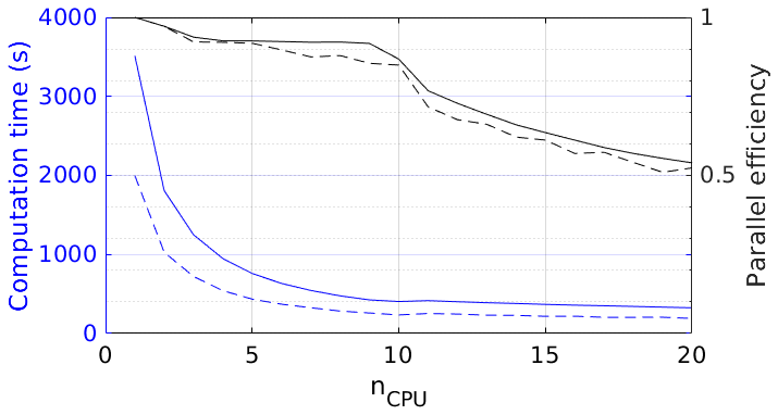
Figure 9 Performance of the parallelized computation depending on the number of core processing units (CPU) used. Model M3-L70-V01 is used with $n_{max}=\mathrm{800}$ (viscoelastic regime), N_grid=6000 and N_t=100 (dashed lines), or N_grid=600 and N_t=1000 (solid lines). Parallel efficiency is defined as the ratio of computation time at 1 CPU to the total core time at n_CPU ($\mathrm{Efficiency}=\frac{\mathrm{Time}(n_{\mathrm{CPU}}=\mathrm{1})}{\mathrm{Time}\left(n_{\mathrm{CPU}}\right)\times n_{\mathrm{CPU}}}$). For example, a perfect efficiency of 1 at n_CPU=20 would indicate that computation time is decreased by a factor 20, while an efficiency of 0.5 would be the result of a factor 10 decrease only.

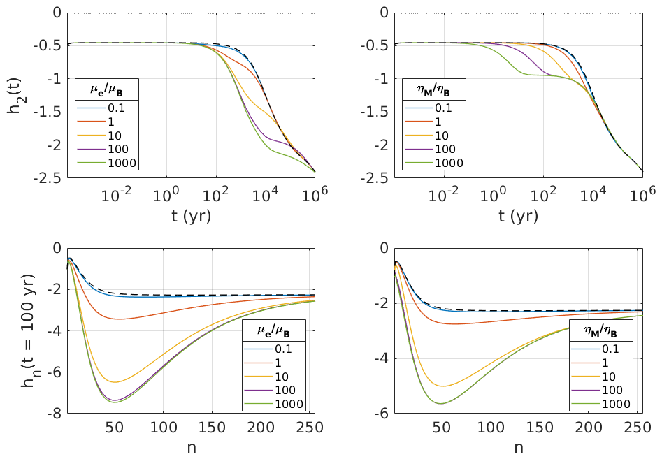
Figure 10 Love numbers based on a variation of the M3-L70-V01 model with simple Burgers rheology instead of Maxwell. Left column: the ratio of shear moduli ${\mathit{\mu }}_{\mathrm{e}}/{\mathit{\mu }}_{\mathrm{B}}$ is varied with the ratio of viscosities ${\mathit{\eta }}_M/{\mathit{\eta }}_{\mathrm{B}}=\mathrm{10}$. Right column: ${\mathit{\eta }}_M/{\mathit{\eta }}_{\mathrm{B}}$ is varied and ${\mathit{\mu }}_{\mathrm{e}}/{\mathit{\mu }}_{\mathrm{B}}=\mathrm{3}$. Top row: time-dependent Love number at degree 2. Bottom row: degree-dependent Love number 100 years after the Heaviside load. The dashed line indicates the Love number response for the same Earth model with Maxwell rheology instead.

6 Transient rheology

Here, we explore the changes to Love numbers when transient deformation is added to a given Maxwell rheology by augmenting it to a simple Burgers or EBM rheology. These transient Love numbers are computed for the incompressible case by replacing μ(s) in the y_i system using the formula indicated in Table 3. We have found that the availability of libraries computing the hypergeometric function ${}_{\mathrm{2}}{F}_{\mathrm{1}}(\mathrm{1},\mathrm{1}+\mathit{\alpha };\mathrm{2}+\mathit{\alpha };z)$ (with in our application $z=-s{\mathit{\tau }}_{\mathrm{H}}$ or $z=-s{\mathit{\tau }}_{\mathrm{L}}$) outside of $-\mathrm{1}<z<\mathrm{1}$ is limited. Therefore, we provide analytical alternatives in Sect. S1 in the Supplement for a select number of values for α. Previous work showcased an EBM response to loading for a half-space model without an elastic lithosphere (Ivins et al., 2020, 2023a) and to tidal forcing (Lau and Schindelegger, 2023). In Figs. 10 and 11, we show loading Love numbers for a variation of model M3-L70-V01 that includes transient relaxation. For each case, we vary linearly or logarithmically one transient parameter at a time; nominal parameters for the simple Burgers rheology are ${\mathit{\mu }}_{\mathrm{e}}/{\mathit{\mu }}_{\mathrm{B}}=\mathrm{3}$ and ${\mathit{\eta }}_M/{\mathit{\eta }}_{\mathrm{B}}=\mathrm{10}$ and for EBM rheology are α=0.5, τ_L=54 min, τ_H=7 years and Δ=3. For simple Burgers rheology (Fig. 10), we note that varying the short term viscosity affects the characteristic time scale of the response, but not its amplitude. On the other hand, the shear modulus μ_B of the Kelvin-Voigt element associated with the transient response affects both properties.

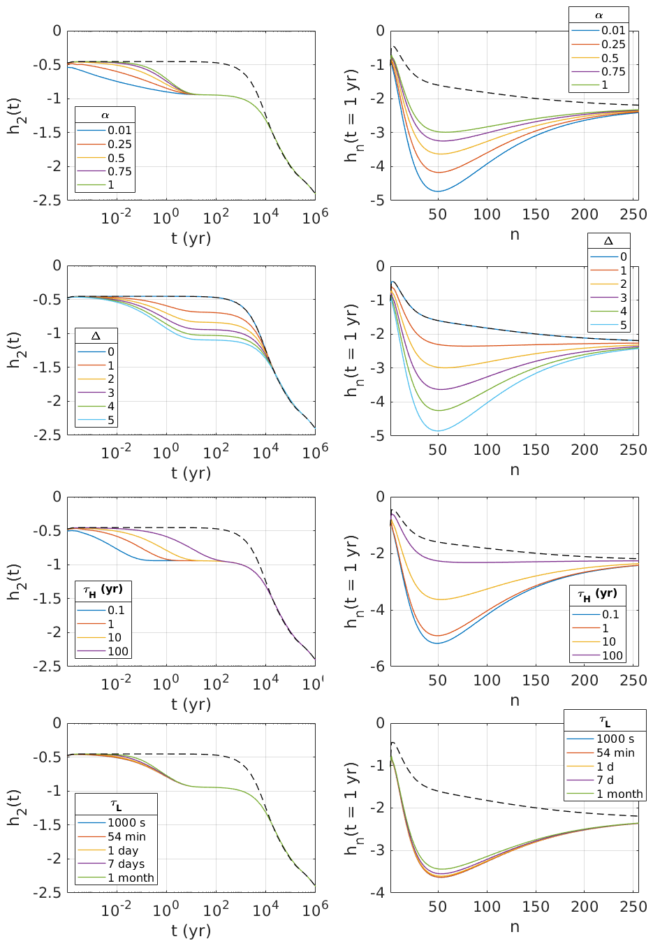
Figure 11 Love numbers based on a variation of the M3-L70-V01 model with the Extended Burgers Material (EBM) rheology instead of Maxwell. Transient parameters are varied linearly one at a time (top to bottom rows), with nominal values α=0.5, τ_L=54 min, τ_H=7 years and Δ=3. Left column: time-dependent Love number at degree 2. Right column: degree-dependent Love number 1 year after the Heaviside load. The dashed line indicates the Love number response for the same Earth model with Maxwell rheology instead.

For EBM rheology (Fig. 11), we remark that the variation of low-cutoff time τ_L within values suggested by the literature (see Ivins et al., 2020, 2023a) only results in minimal changes to Love numbers for all degrees, even for the high value of 1 month. Realistic estimations of τ_L range between ≈1 and 12 h. Below this period, the absorption band associated with long-period seismic normal modes dominates the regime of anelastic dissipation (Lau and Faul, 2019). At a period of 12 h, the M2 tide phase lag (Ray et al., 2001) suggests that large-scale mantle anelasticity is already in effect, implying τ_L<12 h.

We find that variations of α only produce significant changes at time scales below the specified high-cutoff time τ_H, which here essentially results in sensitivity α only at seasonal and shorter periods. However, we do not yet have firm constraints on τ_H, especially for the deep mantle, and it is therefore possible that α could have a significant impact on yearly to centennial time scale especially when τ_H appears to be larger than considered here. In any case, we expect α to be most important for applications related to body tides. The other two parameters Δ and τ_H appear as the main controls to the amplitude and time scale of the response, respectively, which is consistent with the results of Ivins et al. (2023a). We expect these two parameters to be the most important controls in applications of EBM to GIA and contemporary loading problems. It is important to appreciate the role of Δ as an amplification factor for transient behavior, a fact that also holds for the simple Burgers material (SBM) (Faul and Jackson, 2015).

The analogous roles played by the relaxation strength among simple and extended Burger's rheologies motivates inclusion of post-seismic geodetic studies in a summary of our quantitative understanding of Δ. A summary is presented in Table 1 wherin we note that the strength parameter for SBM is $\overline{\mathrm{\Delta }}={\mathit{\mu }}_{\mathrm{e}}/{\mathit{\mu }}_{\mathrm{B}}$ (e.g. Faul and Jackson, 2015; Ivins et al., 2023a). We note that Hines and Hetland (2016) modeled the post-seismic deformation following the 2010 M_w=7.5 El Mayor-Cucapah earthquake with Maxwell rheology and three transient rheologies (Zener, Burgers and the Generalized Maxwell). They concluded that a transient rheology was required to fit the GPS data, and that an optimum ratio of instantaneous rigidity (μ_e) to longer-term rigidity (analogue to μ_B) was determined to be 2.67. We enter this estimate of $\overline{\mathrm{\Delta }}$ into Table 1. It should be kept in mind that the post-seismic models have yet to explicitly consider the EBM rheological formulation.

In Table 1, we include a reanalysis of experiments by Chopra (1997) and Chopra and Paterson (1981) on wet and dry dunite samples. It is interesting that the value for $\overline{\mathrm{\Delta }}$ derived by Masuti and Barbot (2021) for the wet sample is nearly one order of magnitude larger than the Δ value found in the experimental results for dry olivine-pyroxene by Qu et al. (2021). Clearly, there is a great challenge for developing data controlled EBM-based geodynamic models in the future. The new software provided to the geosciences community here may offer an important vehicle for addressing this challenge.

7 Conclusions

Determining the decadal and centennial evolution of the Greenland and Antarctic ice sheets, and the associated sea-level change, informs major decisions for coastal hazard mitigation and social development at the global scale. Such complex systems involve a diverse array of physical processes occurring both within and between ice sheets, terrestrial water, oceans and the solid-Earth. In particular, important feedback loops have been identified in marine-terminating ice sheets between ice thickness change at the grounding line and the viscoelastic bedrock response. The framework presented in this paper offers a way to tackle these problems through the computation of Love numbers, emphasizing the following features:

1. Two-way coupling capability with surface mass transport models is enabled through the Heaviside-response-form of the time-dependent Love number. This is achieved via the Post-Widder approach to the inverse Laplace transform.

2. Computation at very high spherical harmonic degree (>10⁴) is enabled by moving the boundary condition at the innermost interface toward the surface throughout the computation.

3. We provide support for traditional mantle rheology models (elastic, Maxwell and Burgers) as well as the Extended Burgers Material (EBM), an emerging linear rheology model that focuses on describing mantle viscoelasticity between the seismic and Glacial Isostatic Adjustment timescales. All rheologies are supported in the compressible and incompressible regimes.

4. The exploration of rheological parameters, and uncertainty quantification via ensemble modeling approaches are promoted by improvements to the computation time via the optimization of the propagation coefficient matrix, the implementation of parallel computation, and the detection of transition between the viscoelastic and elastic regimes at high degree.

The validation of our results was carried out via comparison with the community benchmark of Spada et al. (2011) for incompressible Maxwell models up to spherical harmonic degree 256. Further work toward benchmarking community capabilities at high spherical harmonic degree, for compressible and transient rheologies is required for additional validation in the corresponding regimes.