darcyInterTransportFoam v1.0: an open-source, fully-coupled 3D solver for simulating surface water – saturated groundwater processes and exchanges

Fully-coupled solvers have proven to be suitable and computationally efficient tools for studying surface water–groundwater (SW-GW) interactions. Most existing fully-coupled codes use the two-dimensional, depth-averaged shallow water equations for surface flows. As a result, three-dimensional (3D) flow dynamics are ignored in the surface domain, including phenomena important for the SW-GW exchange such as turbulence. Computational Fluid Dynamics (CFD) solvers allow to capture 3D information on the surface turbulent flow by solving the full Navier-Stokes equations. Consequently, they are well-suited for the study of the actual exchange flows of water and solutes across the sediment-water interface. Among the available CFD software, the open-source toolbox OpenFOAM provides a flexible modelling framework to implement user-defined, fully-coupled models for the detailed investigation of SW-GW interaction processes. Based on this CFD platform, Lee et al. (2021) developed hyporheicScalarInterFoam, a fully-coupled 3D solver capable of solving the flow and transport processes in both surface and subsurface domains as well as the interactions across their interface. Despite the potential of this new code to tackle SW-GW interactions, its application to real-world hydrogeological scenarios is constrained by limitations in boundary conditions, parameter heterogeneity and key hydrodynamic and transport processes, among others, which hinder the accurate representation of the complex characteristics of natural systems. To overcome this, an updated and extended version of hyporheicScalarInterFoam, called darcyInterTransportFoam, is presented in this paper. The new fully-coupled solver enhances the applicability of the original by introducing novel simulation features. These include internal solver updates, such as the definition of heterogeneous and anisotropic subsurface fields and the simulation of heat transfer in both domains, as well as newly implemented add-ons, including pre- and post-processing utilities and additional boundary conditions. A complete description of all the new features is provided in this paper. Moreover, the utility of darcyInterTransportFoam is demonstrated in a test case, where the SW-GW flow, solute transport and heat transfer processes are simulated in a highly conductive river-aquifer system.

1 Introduction

Acknowledging the role that surface water-groundwater (SW-GW) interactions play for the health of aquatic ecosystems has gained importance in recent years (Brunner et al., 2017; Krause et al., 2017; Lewandowski et al., 2020). Surface water bodies, such as streams, lakes or wetlands, and the aquifers they are connected to should be considered as a single, integral entity due to their continuous interaction (Winter et al., 1998). This interaction controls the fate and transport of contaminants and waterborne substances in the system (Dichgans et al., 2023; Nisbeth et al., 2019; Schaper et al., 2018). Likewise, aerobic and anaerobic reactions as well as the different biological activities produced in the ground are also influenced by this bidirectional exchange (Lewandowski et al., 2019; Nogueira et al., 2021; Trauth et al., 2018). Consequently, the water quality and the overall ecological health of the SW-GW system is affected by the continuous interaction across the sediment-water interface (Boano et al., 2014; Toran, 2019).

Multiple investigations on both water and solute exchange have recently been conducted to study the interconnection between SW and GW (Coluccio and Morgan, 2019; Hermans et al., 2023; Krause et al., 2023). In this context, numerical models arise as a viable complement to field and laboratory experiments to investigate the dynamic interactions across the sediment-water interface (Barthel and Banzhaf, 2016; Brunner et al., 2017; Fleckenstein et al., 2010; Krause et al., 2014). Compared to physical studies, numerical models can provide high-resolution spatiotemporal information on relevant flow and transport processes at any location in the system (Broecker et al., 2021). SW-GW interaction cases are commonly solved using an asynchronous linking, or one-way, coupling approach (Maxwell et al., 2014), with pressure as the coupling parameter (e.g., Chen et al., 2015, 2018; Jin et al., 2011; Lee et al., 2020; Trauth et al., 2014; Trauth and Fleckenstein, 2017). Following this technique, a surface flow model is coupled to a groundwater flow model, where the pressure distribution at the bottom boundary of the surface model is imposed as the upper boundary condition (BC) for the groundwater model. No feedback is provided from the subsurface to the surface domain after solving the groundwater fields, meaning that the resulting exchange fluxes do not influence the surface flow dynamics. However, since flow and transport exchanges are bidirectional, considering the interfacial feedback as unidirectional may result in significant errors in the water and mass balances (Li et al., 2020). In this way, fully-coupled models (FCMs) account for the actual bidirectional interaction between SW and GW by transferring parameter information from one domain to another through an iterative algorithm. This coupling strategy is usually referred to as sequential iterative, or two-way, approach (Maxwell et al., 2014). FCMs commonly solve the subsurface flow using Richards' equation and Darcy's law, while applying the shallow water equations or the Navier-Stokes equations to simulate the surface flow. Unlike the shallow water equations, the Navier-Stokes equations account for turbulence in the surface domain. Turbulence has proven to influence the magnitude of SW-GW exchange and, as such, its detailed computation should not be ignored (Tonina and Buffington, 2009; Voermans et al., 2017). The Navier-Stokes equations are solved by Computational Fluid Dynamics (CFD) models. CFD solvers have the potential to account for the complex three-dimensional (3D) mechanisms of flow dynamics, including turbulence, and therefore, to provide high-resolution information on the flow field characteristics.

Among the different CFD models available to simulate 3D processes, the OpenFOAM (Open-Source Field Operation And Manipulation) software has grown in popularity in recent years (e.g., Broecker et al., 2017, 2021; Lee et al., 2020, 2022; Sobhi Gollo et al., 2022; Trauth et al., 2014, 2015). OpenFOAM (Weller et al., 1998) is a powerful, free and open-source C$++$ toolbox consisting of a comprehensive set of applications (solvers, utilities, boundary conditions, etc.) designed to simulate diverse two and three-dimensional continuum mechanics problems, most prominently including CFD (OpenCFD Ltd., 2024). The main advantage of OpenFOAM over other CFD models is the modular and extensible nature of its code structure. As such, OpenFOAM provides an adequate modelling framework to implement FCMs for the thorough study of the 3D SW-GW processes. Based on this, Li et al. (2020) developed hyporheicFoam. This user-defined model simulates flow and biogeochemical reactions in both surface and subsurface domains as well as the two-way exchange across their interface. The multicomponent reactive transport is modelled in both domains by generic advection-diffusion/dispersion-reaction equations, whereas the standard pimpleFoam solver is used to simulate the surface flow dynamics and a new-coded OpenFOAM solver is applied to solve the saturated groundwater flow. The full coupling between domains is achieved via the mapping of conservative flux BCs at the interface through an iterative scheme. The fact of using a transient, incompressible solver like pimpleFoam to simulate the surface flow implies that hyporheicFoam assumes the water surface is flat, i.e., a rigid-lid (e.g., Chen et al., 2018; Janssen et al., 2012; Jin et al., 2011; Lee et al., 2020). Nevertheless, the water surface in rivers is free to move and can adjust to the topography. In this way, prior studies have shown the impact that a deformable, free surface has on the magnitude of bedform-driven SW-GW exchange, indicating an underestimation of the flux exchanges under the rigid-lid assumption (e.g., Broecker et al., 2019, 2021; Trauth et al., 2014, 2015). To overcome this limitation, a new fully-coupled 3D model, called hyporheicScalarInterFoam, was implemented by Lee et al. (2021). This novel solver switches from pimpleFoam to interFoam to simulate the surface flow dynamics but keeps the same solver as hyporheicFoam for the porous media flow. interFoam (Deshpande et al., 2012) is a two-phase, incompressible, immiscible solver within the OpenFOAM library that uses the Volume of Fluid (VOF) phase-fraction based interface capturing approach (Hirt and Nichols, 1981) for solving the three-dimensional Navier-Stokes equations. This interface tracking method allows modelling the free surface located between the two simulated fluids (i.e., air and water in this case), so that the deformations of the river's water surface can be considered in the computation of the SW-GW exchange. Furthermore, in contrast to hyporheicFoam, hyporheicScalarInterFoam only simulates conservative transport at both domains. Model-specific flux BCs are also mapped at the interface through an iterative algorithm for the full coupling of the two domains.

Despite the potential of hyporheicScalarInterFoam to simulate surface water-groundwater (SW-GW) flow dynamics and transport processes, its applicability to actual hydrogeological contexts is constrained by various modelling limitations, including: (1) the solver does not explicitly calculate any hydrology-related field, such as the specific discharge or the hydraulic head, but solves the surface and subsurface hydrodynamics based on the so-called modified pressure and the volume-averaged velocity. (2) A water height cannot be set at the outlet patch of the surface domain and, therefore, neither can a hydrostatic pressure BC that would allow the flow to leave the simulation domain freely. (3) The adjustable body force required to make the pressure field compatible with periodic BCs is only considered in the calculation of the specific discharge, while both the hydraulic head and the groundwater flux are determined without this additional pressure gradient. (4) The model only allows the specification of homogeneous and isotropic parameter fields (i.e. hydraulic conductivity, porosity and longitudinal and transversal dispersivities) for the entire subsurface domain, which prevents the definition of further complex underground characterizations (e.g., heterogeneous fields). Moreover, (5) the sediment-water interface has to be fully submerged so that the model can run, which implies that both domains must be hydraulically connected all over the interface boundary. (6) The transport of conservative solutes requires to always be solved in both phases in the surface domain, whereas (7) the heat transfer simulation is not available in any of the domains. (8) The mapping of data between the domains is performed via interpolation at their interface boundary, which may result in a loss of information depending on the resolution of both meshes. (9) The convergence of the surface and subsurface results is evaluated by a user-specific maximum iteration loop that does not check the solution mismatch between both domains after each iteration. (10) The model does not allow defining BCs at the interface other than those used for the two-way coupling mode, which complicates its execution in one-way coupling mode. Furthermore, (11) the reinitialization of the data fields at any time of the simulation is only possible through data-preprocessing. Consequently, further development of the code is required to fill all the above-mentioned simulation gaps as well as to extend the solver functionality, so that the model could be applied to different scale SW-GW interaction scenarios.

Hence, this paper introduces an updated and extended version of the hyporheicScalarInterFoam solver, based on the computational fluid dynamics (CFD) platform OpenFOAM. Analogously to the earlier version, the new code, called darcyInterTransportFoam, is an open-source, fully-coupled 3D model aiming at the simulation of flow and transport processes in both surface and subsurface domains, as well as the interactions between them. The latter is achieved through the bidirectional mapping of flux BCs at the domain's interface via an iterative scheme. Moreover, as intended, darcyInterTransportFoam upgrades the applicability of the original solver by extending its modelling capabilities through a series of solver updates and new simulation add-ons. The latter consist of several pre- and post-processing utilities, along with three novel boundary conditions. As for the solver updates, these include, among others, the possibility to simulate passive solute transport in a single phase within the surface domain, the definition of non-uniform underground parameter fields, the automatic specification of impervious regions in the subsurface domain and the simulation of heat transfer in both domains. Furthermore, the structure and organization of the code is also updated to make it more user-friendly. Biogeochemical reactions, targeted by other user-defined, fully-coupled OpenFOAM solvers, such as hyporheicFoam (Lee et al., 2022; Li et al., 2020), cannot be simulated with the current version of the solver, just as they could not in hyporheicScalarInterFoam.

The efficacy of the new solver is additionally demonstrated in a three-dimensional test case, in which the SW-GW flow, solute transport and heat transfer processes occur across a river segment of an actual alluvial system are simulated using darcyInterTransportFoam.

2 Model description

darcyInterTransportFoam (Pardo-Álvarez, 2025, 2026a) is implemented in the free and open-source CFD software OpenFOAM v2412. Similarly to its predecessor, the new fully-coupled solver applies a pseudo-transient coupling approach, in which transient surface flow and steady-state saturated subsurface flow are simulated at every time step (Fig. 1). Accordingly, the subsurface solution is updated at each time step based on the transient BCs firstly computed at the SW-GW interface during the surface flow simulation. After solving the subsurface flow, relevant quantities are mapped back onto the surface domain within the same time step, reflecting the combined effects of the transient surface forcing and any additional subsurface boundary contributions. A convergence check is then performed to ensure consistency between surface and subsurface exchanges after mapping. A similar procedure is applied to solute transport and heat transfer, although in these processes transience is considered in both domains. Due to the different characteristic response timescales of surface and subsurface flows, a single iteration per time step is generally sufficient, unless strong, fast two-way feedback across the interface requires additional convergence loops. Consequently, the subsurface adjustment is assumed to occur quasi-instantaneously, consistent with the slower response of groundwater compared to surface water. This approach reflects the physical assumption that, over the short timescales of surface flow variations, the subsurface water table remains stable and does not undergo significant movement. As a result, the model achieves faster and more stable simulations.

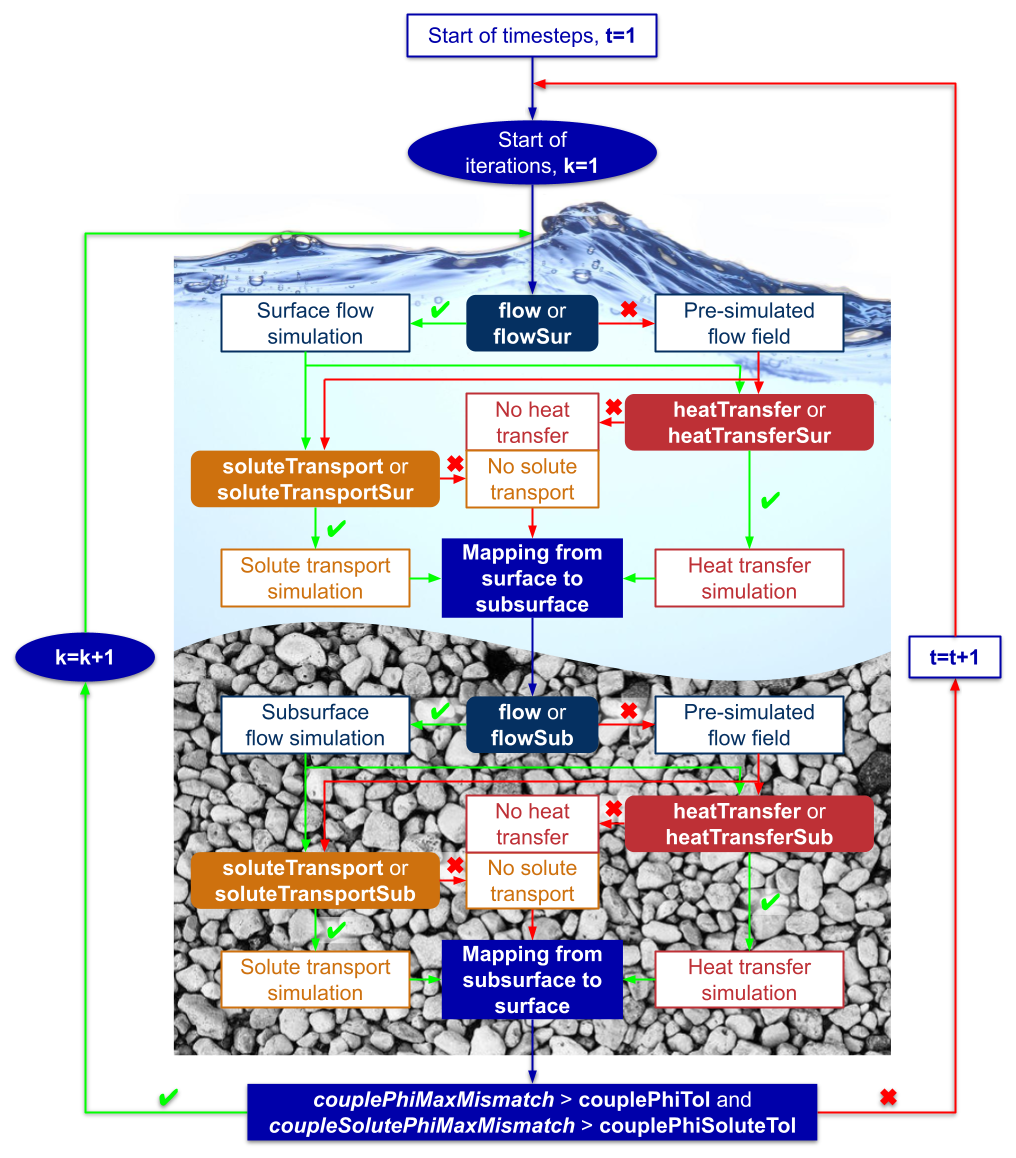
Figure 1 Simulation workflow of darcyInterTransportFoam. Mass conservation is ensured by the updated iterative scheme, that enforces both water and solute flux consistency across the interface of the surface and subsurface domains.

The governing equations and coupling modes of darcyInterTransportFoam are described in this section, followed by an overview of its newly introduced simulation features.

2.1 Governing equations

The new FCM introduces small modifications to some original expressions while expanding the functionality of hyporheicScalarInterFoam by incorporating additional equations and simulation options. In this way, the user-defined code for simulating groundwater flow has been updated to improve accessibility and fully account for the influence of surface dynamics on the subsurface solution. Additionally, modified advection-diffusion-dispersion and novel temperature energy equations are implemented in each domain to respectively enhance the conservative solute transport simulation and enable heat transfer modelling.

Both surface and subsurface partial differential equations are discretized using the Finite Volume Method (FVM) in space and the Finite Difference Method (FDM) in time (Schulze and Thorenz, 2014).

2.1.1 Surface domain

darcyInterTransportFoam models the surface flow as a transient, immiscible, two-phase flow using the VOF interface capturing approach. This method separates the two phases (i.e., air and water) by a continuous, free interface, whose location and shape are determined as a property of the phase fraction field, α_i (–) (Schulze and Thorenz, 2015). Such deformation of the interface allows us to account for the actual flow dynamics in the surface domain, which in turn leads to a correct estimate of the flow, solute and heat exchanges across the sediment-water interface.

Turbulent Two-Phase Flow

As commonly assumed for free-surface fluids, the surface flow is additionally considered to be incompressible (Young et al., 2010). Consequently, there is no need for equations of state to relate the thermodynamic variables (Versteeg and Malalasekera, 2007) and the two-phase flow is adequately governed by the continuity equation (Eq. 1), the Navier-Stokes equations (Eq. 2) and the α_i transport equation (Eq. 6).

The VOF method solves the surface flow dynamics considering the two immiscible phases as one fluid. The resulting single-phase is assumed to be Newtonian and incompressible, according to the physical properties of both surface phases. As a result, the continuity equation can be simplified to:

$$\begin{array}{}\text{(1)}& \mathrm{\nabla }\cdot U_{\mathrm{sur},i}=\mathrm{0},\end{array}$$

and the momentum equation to:

$$\begin{array}{}\text{(2)}& \begin{array}{rl}& {\displaystyle \frac{\partial {\mathit{\rho }}_{\mathrm{sur},i}{U}_{\mathrm{sur},i}}{\partial t}}+\mathrm{\nabla }\cdot \left({\mathit{\rho }}_{\mathrm{sur},i}{U}_{\mathrm{sur},i}{U}_{\mathrm{sur},i}\right)\\ & -\mathrm{\nabla }\cdot \underset{{\mathit{\tau }}_{ij}}{\underbrace{\left[{\mathit{\mu }}_{\mathrm{sur},i}\left(\mathrm{\nabla }{U}_{\mathrm{sur},i}+{\left(\mathrm{\nabla }{U}_{\mathrm{sur},j}\right)}^T\right)\right]}}\\ & =-\mathrm{\nabla }{p}_{{\mathrm{rgh}}_{\mathrm{sur},i}}-g\cdot x_i\mathrm{\nabla }{\mathit{\rho }}_{\mathrm{sur},i}+{\mathit{\rho }}_{\mathrm{sur},i}{S}_{U_{\mathrm{sur},i}},\end{array}\end{array}$$

where U_sur,i and U_sur,j respectively denote the single-phase velocity field in the x and y directions (m s⁻¹), t is the time (s), ρ_sur,i and μ_sur,i are respectively the single-phase density (kg m⁻³) and dynamic viscosity fields (N m⁻²), τ_ij is the deviatoric viscous stress tensor field (N m⁻²), $p_{{\mathrm{rgh}}_{\mathrm{sur},i}}$ is the modified pressure field (Pa) obtained by subtracting the hydrostatic pressure to the static pressure, g is the gravitational acceleration vector (m s⁻²), x_i is the cell position vector field (m) and $S_{U_{\mathrm{sur},i}}$ accounts for any source/sink term field (m s⁻¹). $p_{{\mathrm{rgh}}_{\mathrm{sur},i}}$ enables to avoid potential steep pressure gradients caused by hydrostatic effects as well as simplifying the definition of pressure BCs (Rusche, 2003).

The single-phase parameters ρ_sur,i and μ_sur,i are calculated by weighted averaging of the physical properties of both surface fluids based on α_i:

$$\begin{array}{}\text{(3)}& {\displaystyle }{\mathit{\rho }}_{\mathrm{sur},i}={\mathit{\alpha }}_i{\mathit{\rho }}_{{\mathrm{w}}_{\mathrm{sur}}}+\left(\mathrm{1}-{\mathit{\alpha }}_i\right){\mathit{\rho }}_{{\mathrm{a}}_{\mathrm{sur}}},\text{(4)}& {\displaystyle }{\mathit{\mu }}_{\mathrm{sur},i}={\mathit{\alpha }}_i{\mathit{\mu }}_{{\mathrm{w}}_{\mathrm{sur},i}}+\left(\mathrm{1}-{\mathit{\alpha }}_i\right){\mathit{\mu }}_{{\mathrm{a}}_{\mathrm{sur},i}},\end{array}$$

where ${\mathit{\rho }}_{{\mathrm{w}}_{\mathrm{sur}}}$ and ${\mathit{\rho }}_{{\mathrm{a}}_{\mathrm{sur}}}$ are respectively the densities of the surface water and the air (kg m⁻³) and ${\mathit{\mu }}_{{\mathrm{w}}_{\mathrm{sur},i}}$ and ${\mathit{\mu }}_{{\mathrm{a}}_{\mathrm{sur},i}}$ represent the surface water and air dynamic viscosity fields (N m⁻²). The latter properties result from:

$$\begin{array}{}\text{(5)}& {\mathit{\mu }}_{p_{\mathrm{sur},i}}={\mathit{\mu }}_{{\mathrm{phys}}_{p_{\mathrm{sur}}}}+{\mathit{\mu }}_{\mathrm{turb},i},\end{array}$$

where p is the subscript for the respective surface phase, w (water) or a (air), and ${\mathit{\mu }}_{{\mathrm{phys}}_{p_{\mathrm{sur}}}}$ and μ_turb,i are respectively the physical and turbulent dynamic viscosities (N m⁻²). The μ_turb,i field is computed by the selected turbulence model. As most OpenFOAM solvers, darcyInterTransportFoam allows to choose among different Reynolds-Averaged Navier-Stokes (RANS), Large Eddy Simulation (LES) and hybrid RANS-LES Detached Eddy Simulation (DES) models to simulate the turbulent hydrodynamics. For the test case in this study, the widely applied k-ω SST (Shear Stress Transport) RANS model (Menter, 1994) was chosen to resolve the different scales of turbulence.

An advanced transport equation is used to accurately determine the distribution of α_i through the surface domain and, therefore, the position of the free surface. This is achieved by introducing an additional convective term into the standard α_i transport equation that “compresses” the free surface (Berberović et al., 2009), resulting in a sharper interface resolution which ultimately enables proper conservation of α_i throughout the simulation domain (Weller, 2002):

$$\begin{array}{}\text{(6)}& {\displaystyle \frac{\partial {\mathit{\alpha }}_i}{\partial t}}+\mathrm{\nabla }\cdot \left({\mathit{\alpha }}_i{U}_{\mathrm{sur},i}\right)+\underset{\text{Compression term}}{\underbrace{\mathrm{\nabla }\cdot \left[\right(\mathrm{1}-{\mathit{\alpha }}_i\left){\mathit{\alpha }}_i{U}_{\mathrm{r},i}\right]}}=\mathrm{0},\end{array}$$

where $U_{\mathrm{r},i}=U_{{\mathrm{w}}_{\mathrm{sur},i}}-U_{{\mathrm{a}}_{\mathrm{sur},i}}$ is the relative velocity field (m s⁻¹) between the two surface phases, known as the compression velocity (Berberović et al., 2009).

The resultant α_i is strictly bounded between 0 (air) and 1 (water) in each computational cell of the surface domain. Any value in between will imply a mixture of both phases. As for the interface, the VOF method estimates its location as a property of α_i rather than explicitly computing it, being this normally considered to be around α_i=0.5.

Following the U_sur,i, p_sur,i and α_i solutions, the newly implemented fields of surface water depth, d_sur,i (m), piezometric level, piezo_sur,i (m) and surface hydraulic head, h_sur,i (m), are subsequently calculated according to Bernoulli's equation.

Passive Solute Transport

The new FCM provides two simulation options for modelling the transport of a conservative solute in the surface domain. The first option solves the one-fluid advection-diffusion equation previously implemented in hyporheicScalarInterFoam, based on the formulation introduced by Teuber (2020). Further details on this approach can be found in Haroun et al. (2010), Nieves-Remacha et al. (2015) and Severin (2017).

However, in the new solver the computation of the surface diffusion coefficient field, D_sur,i (m² s⁻¹), differs from that in hyporheicScalarInterFoam in that it also accounts for the contribution of the physical (or molecular) diffusivity, D_phys (m² s⁻¹), to the total diffusivity across the domain, a factor particularly relevant in low-turbulence zones or for fine-scale processes:

$$\begin{array}{}\text{(7)}& D_{\mathrm{sur},i}=D_{\mathrm{phys}}+\left.{\displaystyle \frac{{\mathit{\nu }}_{\mathrm{turb},i}}{{\mathit{Sc}}_{\mathrm{turb}}}}\right\}{D}_{\mathrm{turb},i},\end{array}$$

where Sc_turb is the turbulent Schmidt number (–) and D_turb,i is the turbulent diffusivity, (m² s⁻¹). Both D_phys and Sc_turb have to be defined by the user. Alternatively, D_sur,i can be specified via a constant value for the whole surface domain, offering a simplified yet practical setup not available in the original solver.

The second simulation option is newly implemented and designed to reduce computational costs when the focus is limited to a single simulated phase. Based on the two-phase advection-diffusion equation contained in the standard scalarTransport function object (OpenCFD Ltd., 2023), this approach uses the computed α_i to delimit the extension of the solute transport simulation within the system. Accordingly, the passive transport of any species is only simulated in those cells whose α_i is equal to 1, skipping the rest in the computation. The described governing equation has the subsequent form:

$$\begin{array}{}\text{(8)}& \begin{array}{rl}& {\displaystyle \frac{\partial C_{\mathrm{sur},i}}{\partial t}}+\mathrm{\nabla }\cdot \left({\mathit{\alpha }}_i{U}_{\mathrm{sur},i}{C}_{\mathrm{sur},i}\right)-\mathrm{\nabla }\cdot \left({\mathit{\alpha }}_i{D}_{\mathrm{sur},i}\mathrm{\nabla }{C}_{\mathrm{sur},i}\right)\\ & ={\mathit{\alpha }}_i{S}_{C_{\mathrm{sur},i}},\end{array}\end{array}$$

where C_sur,i is the surface concentration field (kg m⁻³) and $S_{C_{\mathrm{sur},i}}$ accounts for any concentration source/sink field (kg m⁻³).

The latter approach was the one selected to model the conservative solute transport in the test case presented in this paper.

Heat Transfer

Analogously to solute transport, darcyInterTransportFoam enables to solve the surface heat transfer through two new simulation approaches. One of these is based on Aryal (2019) and simulates the distribution of temperature in both surface phases using the following energy equation:

$$\begin{array}{}\text{(9)}& \begin{array}{rl}& \mathit{\rho }{\mathrm{Cp}}_{\mathrm{sur},i}{\displaystyle \frac{\partial T_{\mathrm{sur},i}}{\partial t}}+\mathrm{\nabla }\cdot \left(\mathit{\rho }{\mathrm{Cp}}_{\mathrm{sur},i}{U}_{\mathrm{sur},i}{T}_{\mathrm{sur},i}\right)\\ & -\mathrm{\nabla }\cdot \left(K_{\mathrm{sur},i}\mathrm{\nabla }{T}_{\mathrm{sur},i}\right)=\mathit{\rho }{\mathrm{Cp}}_{\mathrm{sur},i}{S}_{T_{\mathrm{sur},i}},\end{array}\end{array}$$

where ρ is the density (kg m⁻³), Cp_sur,i is the surface specific heat capacity field (m² s⁻² °C⁻¹), T_sur,i is the surface temperature field (°C), K_sur,i is the surface thermal conductivity field (kg m s⁻³ °C⁻¹) and $S_{T_{\mathrm{sur},i}}$ represents any heat source/sink field (°C). As for ρ_sur,i and μ_sur,i, the ρCp_sur,i field is computed as a single-phase property by weighted averaging of ρ and Cp of both phases based on α_i. K_sur,i is likewise evaluated as a function of α_i, with the thermal conductivity of each surface phase, $K_{p_{\mathrm{sur}}}$ (kg m s⁻³ °C⁻¹), defined as:

$$\begin{array}{}\text{(10)}& K_{p_{\mathrm{sur}}}={\displaystyle \frac{{\mathit{\rho }}_{p_{\mathrm{sur}}}{\mathrm{Cp}}_{p_{\mathrm{sur}}}{v}_{{\mathrm{phys}}_{p_{\mathrm{sur}}}}}{{\mathit{Pr}}_{p_{\mathrm{sur}}}}},\end{array}$$

where $v_{{\mathrm{phys}}_{p_{\mathrm{sur}}}}$, ${\mathrm{Cp}}_{p_{\mathrm{sur}}}$, ${\mathit{Pr}}_{p_{\mathrm{sur}}}$ denote, respectively, the physical kinematic viscosity (m² s⁻¹), the specific heat capacity (m² s⁻² °C⁻¹) and the Prandtl number (–) of either the air or water phase.

The second simulation approach restricts the computation of heat transfer to a single surface phase, thereby reducing computational demands. Similarly to solute transport, this is done based on the α_i solution. As such, the transfer of heat is skipped in all those computational cells whose α_i differs from 1. The resulting energy equation has the form of:

$$\begin{array}{}\text{(11)}& \begin{array}{rl}& {\mathit{\rho }}_{{\mathrm{w}}_{\mathrm{sur}}}{\mathrm{Cp}}_{{\mathrm{w}}_{\mathrm{sur}}}{\displaystyle \frac{\partial T_{\mathrm{sur},i}}{\partial t}}+\mathrm{\nabla }\cdot \left({\mathit{\rho }}_{{\mathrm{w}}_{\mathrm{sur}}}{\mathrm{Cp}}_{{\mathrm{w}}_{\mathrm{sur}}}{\mathit{\alpha }}_i{U}_{\mathrm{sur},i}{T}_{\mathrm{sur},i}\right)\\ & -\mathrm{\nabla }\cdot \left(K_{\mathrm{sur},i}\mathrm{\nabla }{T}_{\mathrm{sur},i}\right)={\mathit{\rho }}_{{\mathrm{w}}_{\mathrm{sur}}}{\mathrm{Cp}}_{{\mathrm{w}}_{\mathrm{sur}}}{\mathit{\alpha }}_i{S}_{T_{\mathrm{sur},i}},\end{array}\end{array}$$

As occurred with solute transport, this latter simulation option was chosen to solve the temperature dynamics and exchanges produced in the implemented test case.

2.1.2 Subsurface domain

The introduced solver version assumes the subsurface domain to remain fully saturated, regardless of temporal variations in hydraulic head. Accordingly, groundwater flow is simulated under steady-state conditions, with the solution depending on the transient surface hydrodynamics transferred to the subsurface across the domain interface and on the selected BCs. Subsurface flowpaths, as well as solute and heat processes, are driven by the resulting saturated hydraulic head gradients within the porous medium.

On the other hand, in contrast to the prior solver version, darcyInterTransportFoam defines the subsurface geological parameters, namely, porosity, θ_i (–), hydraulic conductivity, K_ij (m s⁻¹), and longitudinal and transverse dispersivities, α_L,i and α_T,i (m), as 3D scalar and tensor fields. This novel feature allows to extend the applicability of the code to actual alluvial aquifers commonly characterized by heterogeneous θ_i, α_L,i and α_T,i scalar fields as well as heterogeneous and anisotropic K_ij tensor fields.

Saturated Groundwater Flow

Considering the fully saturated assumption, the 3D groundwater flow is described by the following continuity equation for a heterogeneous, anisotropic aquifer:

$$\begin{array}{}\text{(12)}& \mathrm{\nabla }\cdot \left(-K_{ij}\mathrm{\nabla }{h}_{\mathrm{sub},i}\right)=\mathrm{0},\end{array}$$

where h_sub,i is the subsurface hydraulic head field (m). Mass conservation is thus solved based on h_sub,i, in contrast to the modified pressure field, $p_{{\mathrm{rgh}}_{\mathrm{sub},i}}$ (Pa), used in hyporheicScalarInterFoam. While both variables are closely related, they are not identical, as $p_{{\mathrm{rgh}}_{\mathrm{sub},i}}$ does not include the velocity head:

$$\begin{array}{}\text{(13)}& {\displaystyle \frac{p_{{\mathrm{rgh}}_{\mathrm{sub},i}}}{{\mathit{\rho }}_{{\mathrm{w}}_{\mathrm{sub}}}g}}=h_{\mathrm{sub},i}-{\displaystyle \frac{q_i^{\mathrm{2}}}{\mathrm{2}\left|g\right|{\mathit{\theta }}_i^{\mathrm{2}}}},\end{array}$$

where ${\mathit{\rho }}_{{\mathrm{w}}_{\mathrm{sub}}}$ is the groundwater density (kg m⁻³) and q_i is the specific discharge field (m s⁻¹). Consequently, $p_{{\mathrm{rgh}}_{\mathrm{sub},i}}$ approximates h_sub,i in the subsurface, as kinetic energy effects are typically negligible due to the low flow velocities in porous media. However, solving the groundwater flow based on h_sub,i allows for the incorporation of the surface water velocity effects at the SW-GW interface, thereby accounting for their potential influence on the overall subsurface dynamics. This contribution was omitted in the original version of the solver.

Following the head solution, q_i (Haitjema and Anderson, 2016) is sequentially computed using Darcy's law:

$$\begin{array}{}\text{(14)}& q_i=-K_{ij}\mathrm{\nabla }{h}_{\mathrm{sub},i},\end{array}$$

Darcy's law is generally applicable to slow-moving groundwater flows characterized by Reynolds numbers smaller than 10 (Bear, 1972), a condition that is satisfied in most natural groundwater environments. The application of Darcy's law to non-Darcy-flow in porous media may lead to an overestimation of the groundwater flow rates.

Passive Solute Transport

The conservative solute transport in the porous medium is modelled using the same advection-diffusion-dispersion equation as in hyporheicScalarInterFoam. Nevertheless, in darcyInterTransportFoam the hydrodynamic dispersion coefficient tensor field, D_sub,ij (m² s⁻¹), can either be specified as spacially uniform and constant through a single value or calculated as the sum of the effective molecular diffusion coefficient field, D_diff,ij (m² s⁻¹), and the mechanical dispersion coefficient field, D_disp,ij (m² s⁻¹). This choice between two alternatives represents an improvement over its predecessor, where only the second option was available, and aims to provide greater flexibility to the user in solute transport simulations. Moreover, unlike in hyporheicScalarInterFoam, the D_diff,ij tensor corrects for tortuosity the user-defined molecular diffusion coefficient, D_m, based on Boudreau (1996), ensuring a more accurate representation of solute transport in complex subsurface environments:

$$\begin{array}{}\text{(15)}& D_{\mathrm{diff},ij}={\displaystyle \frac{D_{\mathrm{m}}}{\mathrm{1}-\mathrm{2}\ln {\mathit{\theta }}_i}}{J}_{ij},\end{array}$$

where J_ij is the tensor of ones. The D_disp,ij tensor follows the same formulation as in the original solver, with the default setting ${\mathit{\alpha }}_{\mathrm{T},i}=\mathrm{0.1}\cdot {\mathit{\alpha }}_{\mathrm{L},i}$ (Cardenas et al., 2008) applied when no field is specified for α_T,i at the start of the simulation.

Heat Transfer

The new FCM solves the transport of heat at the subsurface domain assuming local thermodynamic equilibrium in the ground. Thus, both the groundwater and the porous medium ($T_{{\mathrm{w}}_{\mathrm{sub}}}$ and T_pm, respectively) are considered to be at the same temperature $T_{{\mathrm{w}}_{\mathrm{sub}}}=T_{\mathrm{pm}}=T_{\mathrm{sub}}$. This assumption simplifies the definition of the heat transfer model to a single energy equation (Rubin, 1974), derived by combining the energy balance equations of both subsurface phases (i.e., water and porous medium):

$$\begin{array}{}\text{(16)}& \begin{array}{rl}& \mathit{\rho }{\mathrm{Cp}}_{\mathrm{sub},i}{\displaystyle \frac{\partial T_{\mathrm{sub},i}}{\partial t}}+\mathrm{\nabla }\cdot \left({\mathit{\rho }}_{{\mathrm{w}}_{\mathrm{sub}}}{\mathrm{Cp}}_{{\mathrm{w}}_{\mathrm{sub}}}{U}_{\mathrm{sub},i}{T}_{\mathrm{sub},i}\right)\\ & -\mathrm{\nabla }\cdot \left(K_{\mathrm{sub},i}\mathrm{\nabla }{T}_{\mathrm{sub},i}\right)=\mathit{\rho }{\mathrm{Cp}}_{\mathrm{sub},i}{S}_{T_{\mathrm{sub},i}},\end{array}\end{array}$$

where T_sub,i is the subsurface temperature field (°C), ${\mathrm{Cp}}_{{\mathrm{w}}_{\mathrm{sub}}}$ is the groundwater specific heat capacity (m² s⁻² °C⁻¹), K_sub,i is the subsurface thermal conductivity field (kg m s⁻³ °C⁻¹) and $S_{T_{\mathrm{sub},i}}$ represents any heat source/sink field (°C). The overall specific heat capacity field, ρCp_sub,i, is computed by weighted averaging of ρ and Cp of the groundwater and the porous medium based on θ_i. K_sub,i is also averaged in the same way, with the thermal conductivity of groundwater, $K_{{\mathrm{w}}_{\mathrm{sub}}}$ (kg m s⁻³ °C⁻¹), calculated analogously to $K_{p_{\mathrm{sur}}}$ and the thermal conductivity of the porous medium, K_pm (kg m s⁻³ °C⁻¹), prescribed by the user as a single constant value. By default, the variables used to compute $K_{{\mathrm{w}}_{\mathrm{sub}}}$ are assigned the values of their surface counterparts, although user-defined values can also be specified.

2.2 Coupling modes between the two domains

Although darcyInterTransportFoam has been initially designed to run in sequential iterative mode (i.e., two-way coupling), the solver also supports application in asynchronous linking mode (i.e., one-way coupling). Both coupling approaches were previously available in hyporheicScalarInterFoam.

Nevertheless, minor updates have been introduced to the sequential iterative coupling scheme to enhance the data transfer between domains, thereby enforcing flux consistency across the interface. These include the code reorganization to improve readability and comprehension, the reformulation of the data mapping approach and the definition of new options for selecting the processes to simulate. Further details on the updates implemented in the two-way coupling scheme can be found in Sect. 2.3.1.

The governing surface and subsurface flow equations are solved sequentially and iteratively within each time step in the updated fully-coupled scheme, as follows:

In the first iteration, k, the surface hydrodynamic fields, namely $U_{\mathrm{sur},i}^k$ and $p_{\mathrm{sur},i}^k$, are first solved using the Navier-Stokes equations to next infer from them $h_{\mathrm{sur},i}^k$.

The estimated $h_{\mathrm{sur},i}^k$ at the bottom boundary of the surface domain is transferred to the top boundary of the subsurface domain (Fig. 2) according to:

$$\begin{array}{}\text{(17)}& \left\{\begin{array}{lll}\mathrm{\nabla }{h}_{\mathrm{sub},i}^k\cdot n_{\mathrm{sub},i}=\mathrm{0}& \Rightarrow & U_{\mathrm{sur},i}^k\cdot n_{\mathrm{sur},i}<\mathrm{0}\left(\text{upwelling flux}\right)\\ h_{\mathrm{sub},i}^k=h_{\mathrm{sur},i}^k& \Rightarrow & U_{\mathrm{sur},i}^k\cdot n_{\mathrm{sur},i}>\mathrm{0}\left(\text{downwelling flux}\right)\end{array}\right.\end{array}$$

where n_sur,i and n_sub,i are, respectively, the outward-pointing unit normal vector field of the surface bottom and subsurface top boundaries.

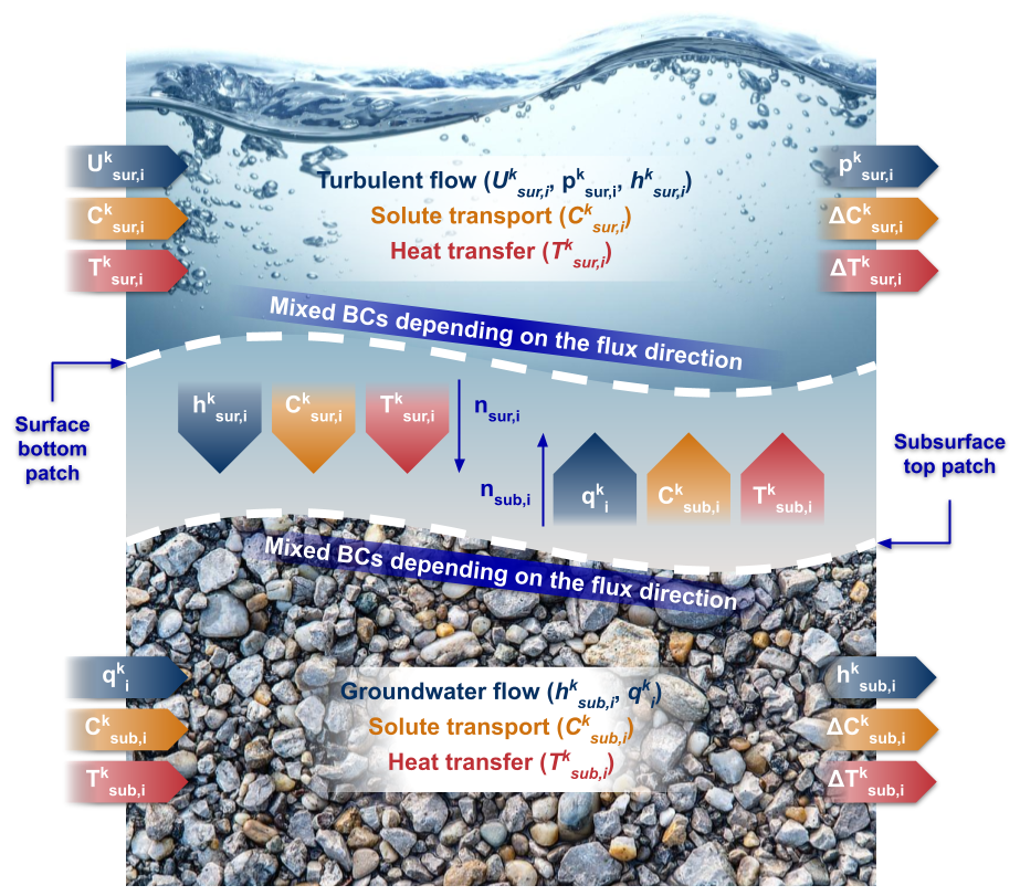
Figure 2 Two-way data mapping at the interface patch of the surface and subsurface meshes for the full coupling of both domains.

The groundwater flow is then simulated using the saturated porous media continuity equation, which results in an estimated $h_{\mathrm{sub},i}^k$ from which an estimated $q_i^k$ is ultimately inferred.

The resulting $q_i^k$ at the upper boundary of the subsurface domain is subsequently mapped to the bottom boundary of the surface domain (Fig. 2). Accordingly, in the next iteration, k+1, the surface bottom BC for $U_{\mathrm{sur},i}^{k+\mathrm{1}}$ will depend on whether the flux is downwelling or upwelling as per:

$$\begin{array}{}\text{(18)}& \left\{\begin{array}{lll}{U}_{\mathrm{sur},i}^{k+\mathrm{1}}=q_i^k& \Rightarrow & q_i^k\cdot n_{\mathrm{sub},i}>\mathrm{0}\left(\text{upwelling flux}\right)\\ \mathrm{\nabla }{U}_{\mathrm{sur},i}^{k+\mathrm{1}}\cdot n_{\mathrm{sur},i}=\mathrm{0}& \Rightarrow & q_i^k\cdot n_{\mathrm{sub},i}<\mathrm{0}\left(\text{downwelling flux}\right)\end{array}\right.\end{array}$$

$p_{\mathrm{sur},i}^{k+\mathrm{1}}$ will be inferred from $U_{\mathrm{sur},i}^{k+\mathrm{1}}$ through a fixed flux BC. The iterative process will proceed until convergence (Fig. 1).

Once the flow field is solved, a similar iterative scheme is applied to both the solute transport and the heat transfer processes. Depending on the direction of the flux at the interface patch, the BC defined for each domain can be either a fixed value or a fixed flux (Fig. 2). Thereby, for each iteration within a time step, the potential temperature BCs at the subsurface top boundary will be:

$$\begin{array}{}\text{(19)}& \left\{\begin{array}{lll}\mathrm{\nabla }{T}_{\mathrm{sub},i}^k\cdot n_{\mathrm{sub},i}=\mathrm{0}& \Rightarrow & U_{\mathrm{sur},i}^k\cdot n_{\mathrm{sur},i}<\mathrm{0}\left(\text{upwelling flux}\right)\\ T_{\mathrm{sub},i}^k=T_{\mathrm{sur},i}^k& \Rightarrow & U_{\mathrm{sur},i}^k\cdot n_{\mathrm{sur},i}>\mathrm{0}\left(\text{downwelling flux}\right)\end{array}\right.\end{array}$$

whereas at the surface bottom patch:

$$\begin{array}{}\text{(20)}& \left\{\begin{array}{lll}{T}_{\mathrm{sur},i}^{k+\mathrm{1}}=T_{\mathrm{sub},i}^k& \Rightarrow & q_i^k\cdot n_{\mathrm{sub},i}>\mathrm{0}\left(\text{upwelling flux}\right)\\ \mathrm{\nabla }{T}_{\mathrm{sur},i}^{k+\mathrm{1}}\cdot n_{\mathrm{sur},i}=\mathrm{0}& \Rightarrow & q_i^k\cdot n_{\mathrm{sub},i}<\mathrm{0}\left(\text{downwelling flux}\right)\end{array}\right.\end{array}$$

As happened to the flow solution (Eqs. 17 and 18), the iterations will continue until the convergence is reached within each time step. The same procedure will be employed by solute transport.

2.3 Code novelties

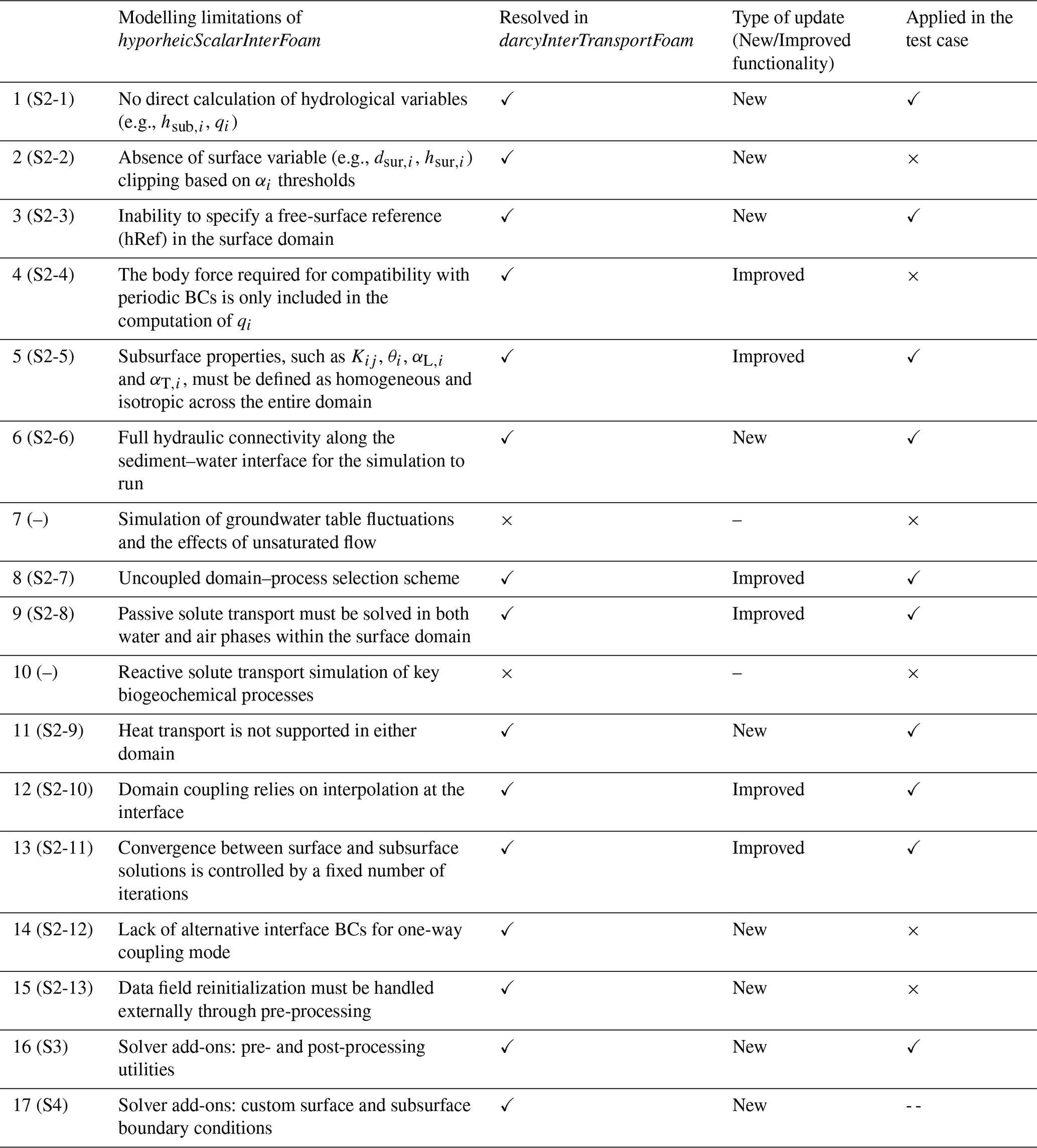
A brief description of the code novelties used in the subsequent test case is provided in the following subsections, while the full set of solver updates and simulation add-ons is indicated in Table 1 and described in detail in the Supplement to this article.

Table 1 Overview of the modelling limitations of hyporheicScalarInterFoam and the corresponding updates implemented in darcyInterTransportFoam, indicating whether each limitation is addressed, the nature of the update and whether the functionality is exercised in the test case. An extended description of each limitation and its associated update is provided in Sects. S2, S3 and S4, with the corresponding point number indicated in brackets in column 1. The marks in columns 3 and 5 denote the status of each entry: a tick for “yes”, a double dash for “partial” and a cross for “no”.

2.3.1 Solver updates

The updates implemented in the solver comprise modifications to the structure and organization of the code (Sect. S1), along with improvements to existing functionalities and the addition of new ones (Sect. S2).

The solver updates described below include the names of all the cited parameters in the code (i.e., files, variables, fields, dictionaries, etc.), along with the corresponding point numbers (in brackets) referring to their extended descriptions in Sect. S2:

Computation of additional hydrology-related fields, such as the specific discharge (q), the water depth (dSur, dSub) or hydraulic head (hSur, hSub). Accordingly, the groundwater flow is solved based on hSub, in contrast to the modified pressure field (pTildeSub) used in the original model (1).

Definition of a reference for the free-surface (hRef) in the surface domain. This optional feature allows to specify a water height at the surface outlet patch that, combined with the appropriate BCs for pressure and velocity, enables the flow to leave the simulation domain freely (3).

Possibility to set the porosity (theta) and the longitudinal and transverse dispersivities (alpha_L and alpha_T) as heterogeneous via scalar fields, as well as the hydraulic conductivity (K) as heterogeneous and anisotropic through a tensor field. This non-uniform field definition provides full flexibility in assigning the previous parameters throughout the subsurface domain, enabling, e.g., the setup of layers with diverse geologic characteristics, a heterogeneous parameter distribution or the definition of impermeable zones (5).

Simplification of the scheme used to select the processes to be solved by the model. As a result, the choice of the flow, the solute transport as well as the heat transfer simulation can be made jointly for both surface and subsurface domains (flow, soluteTransport and heatTransfer options in the simulationProperties dictionary, respectively). Furthermore, as an alternative to this joint selection, the simulation of each process can be also separately specified for each domain. The different process selection options as well as their corresponding implications can be checked in Fig. 1 (7).

Full reformulation of the passive solute transport module, including both the code organization and the modelling approach. Regarding the later, both the surface diffusion and the subsurface hydrodynamic dispersion fields (DSur and DSub, respectively) can be either computed through new or partially modified equations or specified as uniform throughout the domain via a single value (constDSur or constDSub). Moreover, the transport of conservative solutes (CSur) can be optionally solved in one or two phases at the surface domain (solutePhases). All the solute transport related expressions are gathered within the corresponding header files CSurEqn.H and CSubEqn.H in the surface and subsurface domains. A thorough description of the novel transport equations is provided in Sect. 2.1.1 and 2.1.2 (8).

Addition of a heat transfer module for the simulation of the temperature distribution in both surface and subsurface domains. Both the code organization and the modelling scheme of this new module are based on those implemented in its solute transport counterpart. Consequently, two phase-based simulation options (heatPhases) are included in the TSurEqn.H file to simulate the transfer of heat in the surface domain (TSur), whereas the energy equation required to resolve the temperature distribution in the ground (TSub) is contained in TSubEqn.H. Further details about the implemented heat transfer equations can be found in Sect. 2.1.1 and 2.1.2 (9).

Modification of two-way data mapping (Sect. 2.2) for a more accurate conveyance of the information between the domains. In this way, the data is no longer interpolated but directly assigned to the matching nodes of both meshes at their respective interface patch. This new method ensures the exact transmission of the solution from one domain to another (hSur, q, CSur/CSub and TSur/TSub) (10).

Reformulation of the convergence check at the SW-GW interface. Rather than relying on a fixed maximum number of correction loops, water and solute flux consistencies are evaluated at each time step by comparing the exchange fluxes predicted from the surface domain with those computed from the groundwater solution. Convergence is considered achieved when both water and solute flux mismatches (couplePhiMaxMismatch and coupleSolutePhiMaxMismatch) fall below the specified tolerances (couplePhiTol and couplePhiSoluteTol) (Fig. 1) (11).

2.3.2 Pre- and post-processing utilities

Four new utilities were developed to be used with darcyInterTransportFoam (Sect. S3). Additionally, some of them are also compatible with other OpenFOAM solvers. The complete new set was used to perform pre- and post-processing actions in the implemented test case:

checkMeshesMatch: checks whether the number of faces of both meshes and their coordinates match at the interface patch. The fulfilment of both conditions ensures the appropriate fitting of both surface and subsurface meshes. Only applicable to OpenFOAM models consisting of two adjacent simulation meshes.

changeZRefMesh: performs two optional actions: (1) translation of the mesh points according to a user-specified reference mesh elevation; and (2) adjustment of hRef to the actual mesh location. Both actions are independent of each other. Applicable to further OpenFOAM models.

restoreZRefMesh: initially designed to be used in combination with changeZRefMesh but also applicable on its own. This utility conducts three optional and independent actions: (1) translation of the mesh points according to the meshShiftZ value; (2) reestablishment of the original, user-defined hRef (if previously applied changeZRefMesh); and (3) adjustment of the computed hydrological fields (piezoSur, hSur and hSub) based on meshShiftZ. meshShiftZ can be either previously determined by changeZRefMesh or provided by the user in the constant directory. Applicable beyond darcyInterTransportFoam.

transferMeshDecomp: transfers the domain decomposition from one mesh to another through the interface patch of both meshes. A prior decomposition of both domains (decomposePar utility) is required to generate the necessary cellDist and cellDecomposition files for its execution. Furthermore, it optionally overwrites the cellDecomposition file of the reference and/or target mesh once the transfer is done. Only applicable to OpenFOAM models consisting of two adjacent modelling meshes.

2.3.3 Surface and subsurface boundary conditions

One new boundary condition for U_sur,i and another two for h_sub,i were implemented along with the new solver (Sect. S4). Analogously to the novel utilities, some of the new BCs are darcyInterTransportFoam-specific while others can also be applied to other OpenFOAM solvers. The two h_sub,i boundary conditions were used in the test case:

darcyGradHead: sets at the patch the ∇h_sub,i resulting from the defined q_i BC. It is based on the previously developed darcyGradPressure BC (Horgue et al., 2015). Applicable to OpenFOAM models other than darcyInterTransportFoam.

surfaceHydrostaticHead: specifies at the inlet, outlet or aquifer (i.e., bottom) patch of the subsurface domain the hydrostatic h_sub,i computed at the equivalent surface boundary. Accordingly, single values will be assigned to the subsurface inlet and outlet patches ($max\left({\mathrm{piezo}}_{\mathrm{sur},i}\right))$, whereas an entire head field will be prescribed to the bottom boundary of the subsurface domain (piezo_sur,i). In this early version, its use is restricted to the above-mentioned boundaries. Only applicable to darcyInterTransportFoam.

3 Test case

The performance and capabilities of darcyInterTransportFoam are demonstrated through a 3D test case, where the SW-GW flow, solute transport and heat transfer processes are simulated across a segment of an actual, alluvial river-aquifer system. A small description of the simulation domain, the simulated hydraulic scenario and details of the overall modelling setup are provided below.

3.1 Simulation domain

To ensure the necessity of fully-coupled modelling for capturing the full dynamics of the system, a field site characterized by high K_ij values was selected to conduct the evaluation test case. The simulation domain focuses on a segment of the Emme River near Aeschau in the Emmental region of Switzerland (Fig. A1 in the Appendix). At this location, the river features a coarse gravel bed underlain by quaternary alluvium composed of coarse sandy gravel with a variable proportion of silt (Käser and Hunkeler, 2016; Peel et al., 2022). This geology creates an extremely conductive river-aquifer system (Blau and Muchenberger, 1997; Schilling et al., 2017), with depth-averaged K_ij values ranging from $\mathrm{2.3}\times {\mathrm{10}}^{-\mathrm{3}}$ to $\mathrm{7}\times {\mathrm{10}}^{-\mathrm{3}}$ m s⁻¹ and θ_i values between 0.1 and 0.3 (Schilling et al., 2022; Würsten, 1991). The high permeability of the alluvium results in continuous SW-GW interactions across the riverbed (Tang et al., 2018). These exchanges significantly impact the groundwater mixing ratios and travel times, particularly during high-flow events, when the river discharge can account for up to 90 % of the total aquifer recharge (Poffet, 2011; Popp et al., 2021). Together, the described geological and hydraulic characteristics create a highly dynamic river-aquifer system, ideal for testing and evaluating the new fully-coupled SW-GW OpenFOAM model. Further details on the field site characteristics are provided in Käser and Hunkeler (2016) and Schilling et al. (2017).

3.2 Hydraulic scenario

A 8-well abstraction plant (BR1 to BR8) is situated on the extensive floodplain along the river's left bank (Blanc et al., 2024; Schilling et al., 2017, 2022) (Fig. A1). At the end of 2018, two temporary vertical wells (VB1 and VB2) were drilled in the vicinity of this existing wellfield to conduct a major, 1.5-month pumping test (Peel et al., 2022; Popp et al., 2021). Throughout the test, all or part of the water pumped from the two newly installed wells was discharged into the Emme via several pipes (Fig. A2). The mean river temperature during the experiment was 2 °C, while the temperature of the abstracted groundwater averaged 8 °C, coinciding with the mean annual air temperature at the site (Figura et al., 2013). Both surface and subsurface temperatures were obtained from point measurements taken on-site. The resulting plume from the temperature contrast, along with the heat exchange results from previous studies at the site, provides an ideal scenario to test the newly implemented heat transfer module of darcyInterTransportFoam. Consequently, this scenario is selected for the model's test case. Furthermore, although no solute measurements were taken in the river during the pumping test, the solute exchanges are also simulated, assuming similar interaction dynamics as heat across the SW-GW interface.

3.3 General modelling setup

3.3.1 Mesh features

The surface and subsurface meshes for the test case were generated using blockMesh, one of the mesh generation utilities of OpenFOAM. Accordingly, the resulting meshes consist of 3D, structured, hexahedral blocks defined by either straight or curved edges. To enable full control over the mesh generation process, the blockMeshDict file required for running blockMesh was generated for each mesh using a set of user-defined MATLAB scripts (Pardo-Álvarez, 2026b). These scripts were also used to generate other mesh-related dictionaries (e.g., topoSetDict) and input data files (e.g., setFieldsDict) associated with the resulting structured meshes.

Figure 3 Simulation meshes generated with blockMesh.

A high-resolution (0.25 m) Digital Elevation Model (DEM), acquired on 20 March 2015 using drone-based photogrammetry (Schilling et al., 2017), was used to define the interface boundary of both domains (i.e., the riverbed patch) (Fig. A3). The surface and subsurface meshes are approximately 2.5 and 10 m high, respectively, and both are about 235 m long and 50 m wide. However, rectangular inflow and outflow stretches of around 6.25 and 12.5 m long, respectively, were added to each mesh to prevent potential perturbations caused by the geometric features of the inlet and outlet boundaries. Moreover, the smooth transition between these regular sections and the actual riverbed topography was achieved through approximately 12.5 m long segments. Consequently, the total length of each mesh was increased by around 43.75 m (Fig. A3). The other two dimensions remained unaltered.

As for the mesh discretization, a mesh sensitivity study was conducted to determine the optimal resolution for each mesh, leading to the selection of a surface mesh with approximately 2×106 cells and a subsurface mesh with about 8×106 elements. Identical cell counts in the longitudinal and transversal directions are imposed for both domains to ensure effective interface node matching and, thus, successful coupling of their solutions.

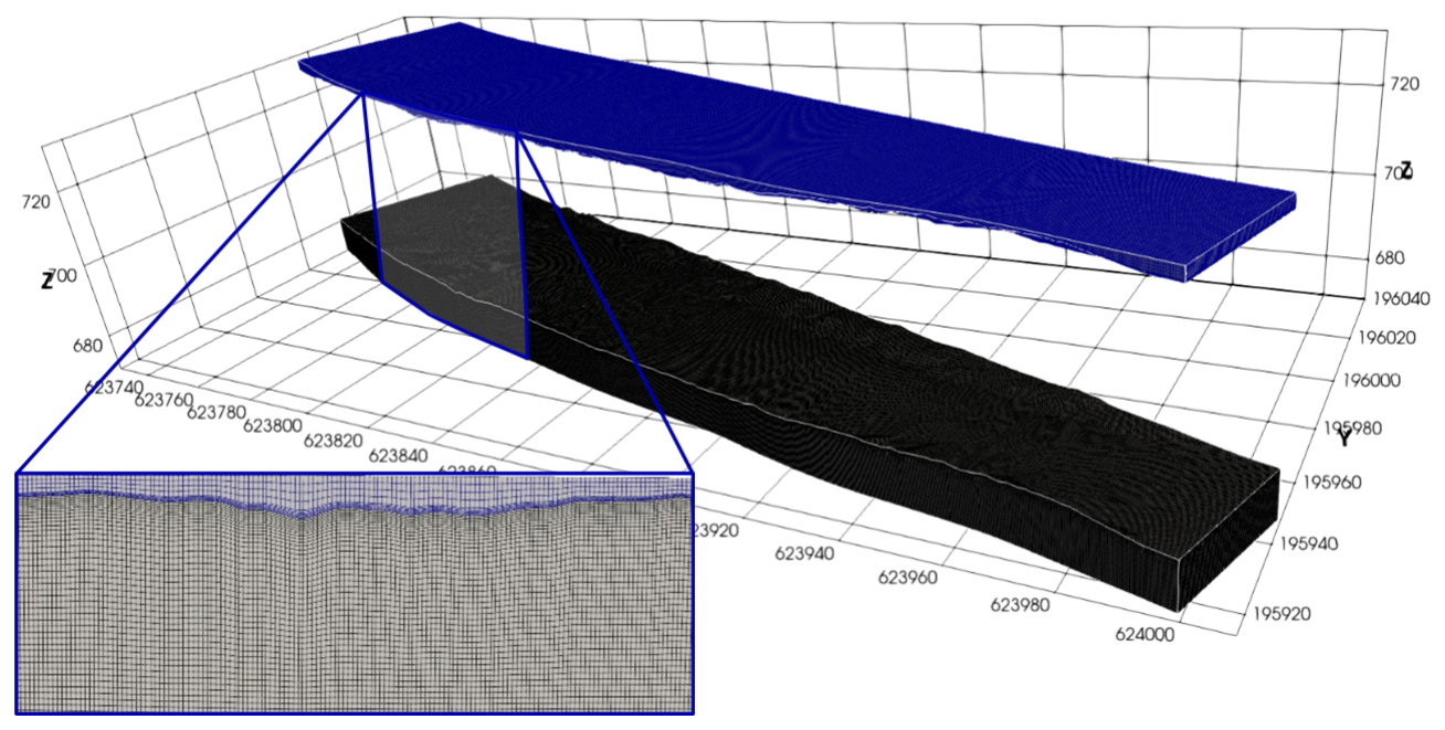
Moreover, the meshes were gradually refined vertically towards the SW-GW interface to capture the complex dynamics across this boundary and satisfy the y+ (dimensionless wall distance) requirement near the riverbed in the surface domain (Fig. 3). In both meshes, the smallest elements are located close to the interface (0.001 m² face area), while the largest cells are situated within the air-phase in the surface domain (0.24 m²) and at the bottom boundary in the subsurface domain (0.1 m²). Especially large element sizes were defined for the surface air-phase, since detailed processes in this region are not of interest for the present study. This phase is only simulated to account for the water level fluctuations.

3.3.2 Model parametrization

All fluid parameters were assumed to stay constant over time in agreement with the simulated steady-state flow and transport dynamics. Common values of ${\mathit{\nu }}_{{\mathrm{phys}}_p}$ and ρ_p at ambient temperature were defined for the air and water (Table A1 in the Appendix). Regarding the solute transport parameters, a D_phys of $\mathrm{4.2}\times {\mathrm{10}}^{-\mathrm{10}}$ m² s⁻¹, corresponding to fluorescein sodium (NaFl), and a Sc_turb of 1 were applied to both surface fluids. D_m was assumed to be equal to D_phys. Moreover, heat parameters, such as Pr_p, were inferred from the fluid temperatures specified for each domain. Further details on the fluid properties are provided in Table A1.

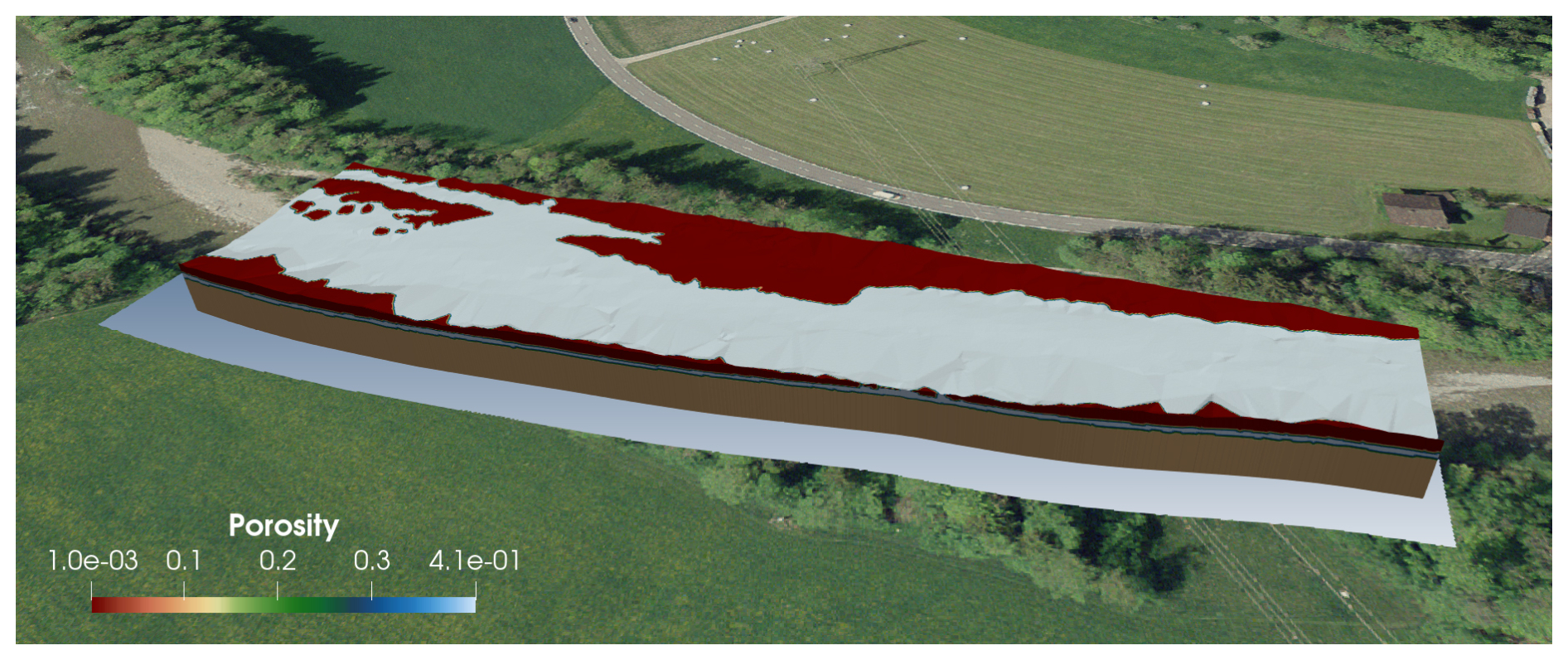
Figure 4 Porosity field (θ_i) of the test case (background image from © Google Maps 2024).

Regarding the geological properties, two layers of different homogeneous and isotropic K_ij and θ_i were defined in the subsurface domain (Fig. 4). The upper layer, located at the first 2 m beneath the riverbed, has a K_ij of $\mathrm{2.8}\times {\mathrm{10}}^{-\mathrm{3}}$ m s⁻¹ and a θ_i of 0.41. These values were assigned via a setFieldsDict using a triangulated surface geometry. The rest of the aquifer corresponds to the second layer, whose K_ij and θ_i are $\mathrm{6.4}\times {\mathrm{10}}^{-\mathrm{3}}$ m s⁻¹ and 0.1, respectively. Moreover, eight impermeable regions of different depths (from 0.25 to 1 m) were defined below the surface dry areas (i.e. the riverbanks and several gravel bars) by means of a triangulated surface geometry using the water table height as reference (Fig. 4). Within these regions, the values of K_ij and θ_i are small enough to ensure the flow cannot pass through them. Thereby, K_ij is set to 10⁻²⁰ m s⁻¹ and θ_i to 10⁻³. Additional geological parameters, such as α_L,i and α_T,i, were also prescribed at the aquifer. In this way, a different homogeneous α_L,i was assigned to each subsurface region. Particularly, α_L,i of 3 and 5 m were set, respectively, to the upper and lower layers, while a field of 10⁻⁷ m was prescribed to the impervious zones. α_T,i was approximated by $\mathrm{1}/\mathrm{10}$ of α_L,i. The rest of the ground parameters can be found in Table A1.

3.3.3 Initial and boundary conditions

All surface and subsurface fields were initialized with values as close as possible to the expected solution to help the model reach the steady state faster. Some values were obtained from a spin-up run, and thus directly specified in the field data files for the entire simulation domain (Tables A2, A3 and A4), while others were assigned to specific mesh locations through different setFields actions. The latter was the case of the surface fields alpha.water (α_i), U (U_sur,i), C (C_sur,i) and T (T_sur,i).

On the other hand, as it happened with the fluid and geologic properties, all the prescribed boundary conditions remained constant during the simulation to represent a steady-state scenario. The inlet of the surface domain is split into two patches, with α_i prescribed accordingly on each one: water enters the domain through the lower patch (inletWater) via a specified constant discharge (10 m³ s⁻¹), whereas the upper half (inletAir) is reserved for the air flow by means of a total pressure condition. The latter condition is also applied to the top boundary (atmosphere). Additionally, water also flows into the domain through the waterJet patch (0.42 m³ s⁻¹). The water level at the surface outlet (0.25 m) is fixed by combining a hydrostatic pressure condition with a reference free-surface elevation (hRef). At the riverbed, U_sur,i is initially set to 0 m s⁻¹, switching to a heterogeneous field after the first coupling iteration. The impact of the riverbed roughness in the flow dynamics is also considered through the application of a rough wall function to ν_turb,i at this patch. As for the subsurface domain, the inlet and outlet boundaries are prescribed with an upstream q_i of $\mathrm{2}\times {\mathrm{10}}^{-\mathrm{5}}$ m s⁻¹ and a downstream hydrostatic h_sub,i condition, respectively. Furthermore, h_sub,i is originally fixed to zero at the riverbed, pending the first iteration of the coupling scheme to change its value. Regarding the solute transport and heat transfer simulation, constant input values of 5 kg m⁻³ and 2 °C are set at the inletWater patch and 10 kg m⁻³ and 8 °C at the waterJet and subsurface inlet boundaries, whereas both inletAir and atmosphere patches are prescribed with a zero-gradient outflow condition with specified input for the case of reversing flow. Similar mixed BCs are defined at the riverbed in the two domains, mapping the values from the coupled domain in case of inflow. Both surface and subsurface outlet patches are set to a zero-gradient condition. The remaining boundaries, namely banks and aquifer, are specified as impermeable using a slip condition. As such, the flow can move along the patch but not across it.

The full suite of initial and boundary conditions prescribed for the test case is detailed in Appendix A. For more detailed information on their use and implementation, refer to the online OpenFOAM User's Guide (OpenCFD Ltd., 2023).

3.3.4 Numerical schemes, linear solvers and solution algorithms

The terms of the partial differential equations governing the flow, solute transport and heat transfer are transformed into algebraic equations through different spatial and temporal discretization schemes. The complete suite of numerical schemes used in the present test case can be checked in Table A5.

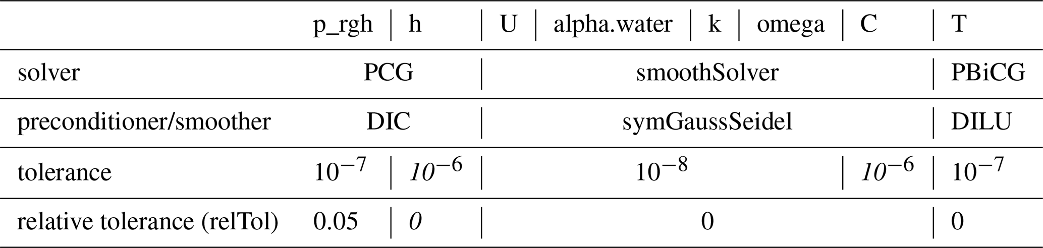
The discretized equations are then solved using a range of iterative linear-solvers. The selected linear-solver, along with the preconditioner and tolerance needed to achieve an accurate solution, is defined for each dynamic variable in Table A6.

In the surface domain, the 3D velocities and pressure are solved iteratively using the PIMPLE pressure-velocity coupling algorithm (OpenCFD Ltd., 2023). This iterative procedure is necessary for the VOF method to effectively solve the pressure field while satisfying the continuity equation. The pressure correction is achieved via the Poisson equation, with convergence attained through 3 inner-correctors and 1 outer-corrector. As for the subsurface solution, the hydraulic heads are corrected for mesh non-orthogonality using 1 non-orthogonal corrector.

The model setup is completed with the definition of the simulation control options. The initial timestep was set to 0.001 s, allowing a maximum timestep of 1 s. Moreover, the timestep size was dynamically adjusted according to a specified maximum Courant number of 0.5 and a maximum alpha Courant number of 1.

4 Results

The test case is defined as a 3D, partially open system. Consequently, water fluxes enter and exit the modelling domain only through the upstream and downstream boundaries, while the riverbanks and aquifer bottom are considered impermeable. This simplified assumption improves upon the 2D, closed model setups of Li et al. (2020) and Lee et al. (2021) by better capturing the dynamic behaviour of a natural river. Furthermore, the defined system aligns with the need expressed by Li et al. (2020) to further study the performance of FCMs in open systems.

Based on the fact that the original model, hyporheicScalarInterFoam, already proved its efficacy to tackle the hydrodynamics of the hyporheic zone, the reach-scale interfacial exchanges are shown this time, together with their overall impact in the whole system dynamics. The selected scale aims to demonstrate the potential of the new model to also untangle the flow dynamics and transport processes at larger hydrological contexts than the hyporheic region.

Since both the conservative transport and heat transfer do not influence the flow, the steady, pre-simulated flow field was used throughout an intermediate period of the simulation (area coloured in the graphs) to speed-up the computational times of both processes.

A selection of the most representative results from the test case is presented in this section. The simulated flow exchanges across the riverbed and associated groundwater flowpaths, along with their impact on the solute concentration and water temperature, are shown and discussed below.

4.1 Exchange water fluxes across the riverbed

Figure 5 illustrates how the groundwater flowpaths cross diagonally the domain, moving from the right to the left bank as they travel through the aquifer. Moreover, they do not avoid the natural riverbanks, but flow underneath as a consequence of the subsurface characterization (Sect. 3.2.2). The length of the resulting flowpaths is directly related to the described directions, being possible to find values ranging from 5 to 170 m. Both physical and geological features of the system explain this fact. In this regard, a shallow channel is formed on the left side of the riverbed as a result of the significant height variation along its cross-section (Fig. A3). Such topographical difference causes a head gradient that drives most of the groundwater flowpaths of the domain. Rather than flowing straight, the paths change their direction towards the left bank of the river. This fact, along with the permeable riverbanks, generally makes the flow travel longer distances than if moved longitudinally under the course of the river. Furthermore, the same system characteristics favour the existence of a broad set of smaller path lengths generated by the multiple gradients produced across the riverbed. A 3D view of the groundwater flowpaths underneath the riverbed is shown in Fig. A4.

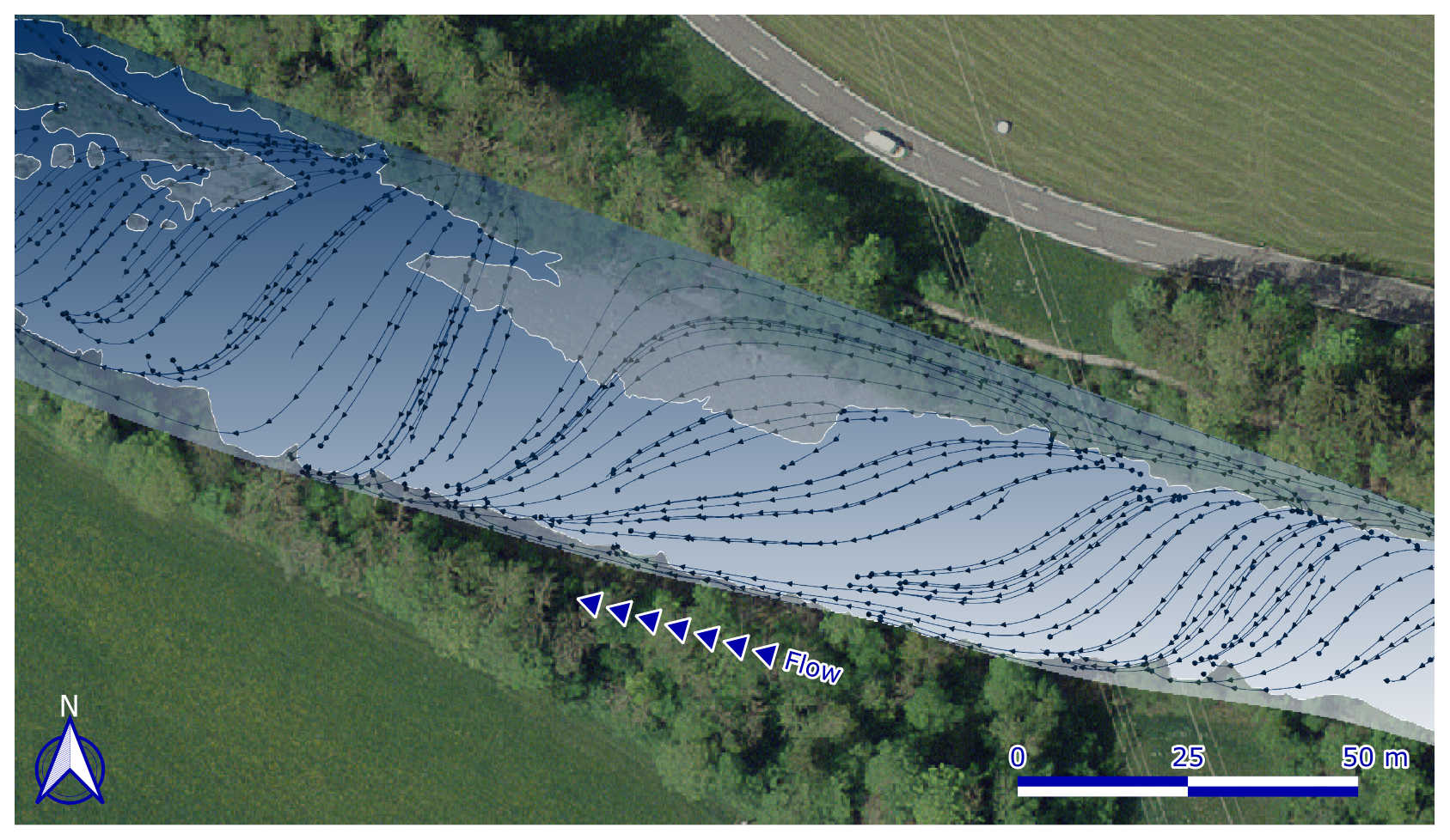
Figure 5 2D top-view of the simulated groundwater flowpaths underneath the riverbed (background image from © Google Maps 2024).

As required, the water balance is conserved within the system. This fact is verified by the surface and subsurface effluxes, that equalled the water influxes once the steady-state was reached. Such conservation of mass confirms the good functioning of the coupling iterative scheme of darcyInterTransportFoam. On the other hand, the exchange fluxes across the riverbed show higher upwelling rates than downwelling (0.34 and 0.28 m³ s⁻¹, respectively), indicating that the exfiltration towards the river prevails over the infiltration into the ground. This pattern is confirmed by the conservative solute and temperature results presented in the following sections.

4.2 Water temperature field

Both the SW-GW heat exchanges and the groundwater plume generated in the river during the pumping test were modelled to evaluate the efficiency of the novel module.

The specified initial temperatures correspond to the mean values measured in-situ during the pumping experiment. Accordingly, the air and water phases in the surface domain were initially set to −2 and 2 °C, respectively, while the groundwater temperature was initialized to 8 °C.

The simulated plume was compared to that measured on site using a drone-mounted thermal camera. As shown in Fig. 6, both drone-based (panel a) and model-based (panel b) outcomes depict the temperature contrast generated by the warm abstracted groundwater. However, while the trajectory and location of the plume look similar in both images, the shape and length differ between them. The reasons behind these differences can be diverse and go from the lack of accurate field observations to a wrong selection of the simulation parameters, or even a combination of both. In this case, the high-flow conditions presented in the river the day the thermal flight was carried out made the acquisition of additional field data especially difficult. This fact reduced the availability of in-situ temperature measurements and, consequently, the capability to later validate the values observed with the drone. Moreover, access to detailed information on the discharged groundwater was challenging due to the engineering approach of the data source. In most cases, the companies responsible for the pumping test provided data at hourly or even daily intervals. These temporal resolutions – far from those required to thoroughly study highly dynamic processes like temperature – combined with the described on-site data limitations, complicated the definition of a suitable model setup for reproducing the temperature field captured by the drone. However, despite these constraints, the model reproduces the overall spatial pattern of heat redistribution, indicating an adequate functioning of the new solver's heat transfer module, while local discrepancies in magnitude remain, as reflected by a root mean square error (RMSE) of 0.82 °C. The mismatch with the observed values can be attributed to a suboptimal selection of the simulation parameters, suggesting that an improved choice would lead to a better match.

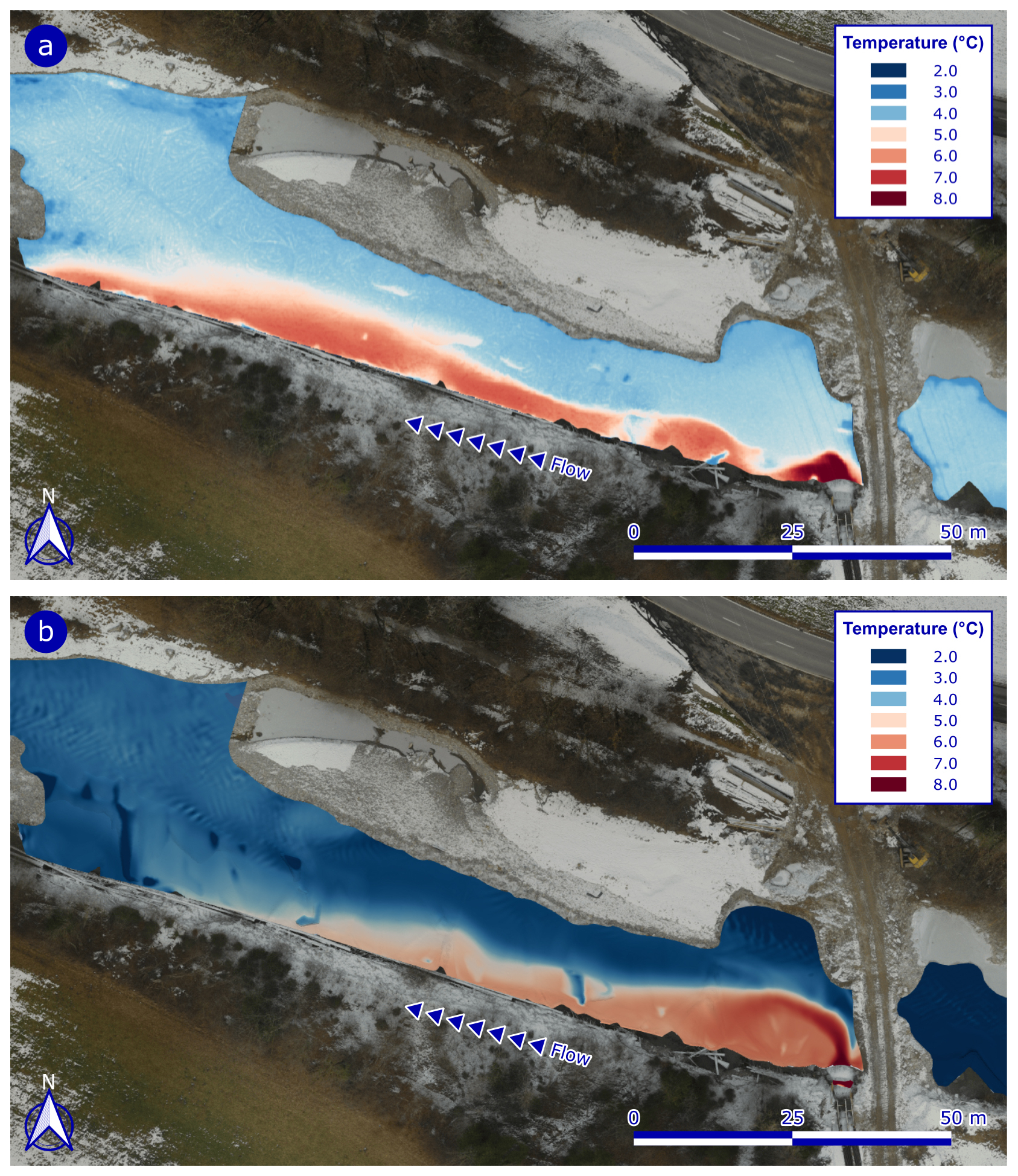
Figure 6 (a) Drone-measured and (b) simulated temperature plumes generated by the groundwater jet at the water surface (background image captured on site by the drone).

As for the heat exchanges across the riverbed, the results obtained show that the two-way exchange mostly occurs across the main course of the river, namely, the shallow channel located on the left side of the bed (Fig. 7a). Within this region, areas of warm groundwater are combined with areas of cold surface water. No groundwater contribution is produced outside of this zone. The resulting temperature pattern aligns with that described in previous studies at the site. One of these, Käser and Hunkeler (2016), identified an alternate sequence of upwelling and downwelling locations along the Emme which proved the existence of a complex pattern of river-aquifer interactions. The outcomes achieved with the new model reproduce such pattern, corroborating in this way the capability of darcyInterTransportFoam to solve actual heat transfer processes.

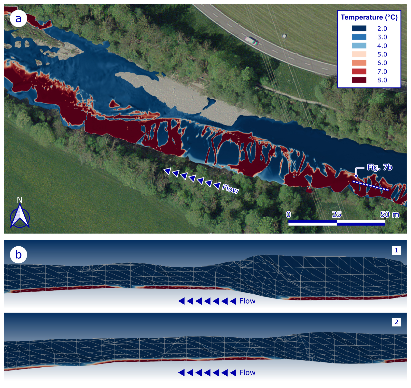
Figure 7 (a) Modelled water temperature pattern at the riverbed (background image from © Google Maps 2024) and (b) cross-sectional view in the x-z plane along the dashed line in (a).

Furthermore, the heat outputs also indicate that, despite the multiple interactions produced across the riverbed, their impact in the surface and subsurface water temperatures is relatively small, as shown in Fig. 8. This figure illustrates how the average temperatures stay nearly constant over time at the outlet of both domains. Such steady behaviour can be explained by the small magnitude of the riverbed exchanges (Sect. 4.1). As a result of this, the tiny gaining fluxes infiltrate in the ending domain just a few millimetres (first row of cells) before mixing with the main flow of the system (Fig. 7b). The big difference in volume between the two flows makes the temperature of the former to diffuse within the second, consequently minimizing its effect in the mean temperature of the domain. These little heat infiltrations would also explain the measuring approach followed by Käser and Hunkeler (2016), that required from near-bed measurements to properly detect the temperature changes resulting from the subsurface upwelling.

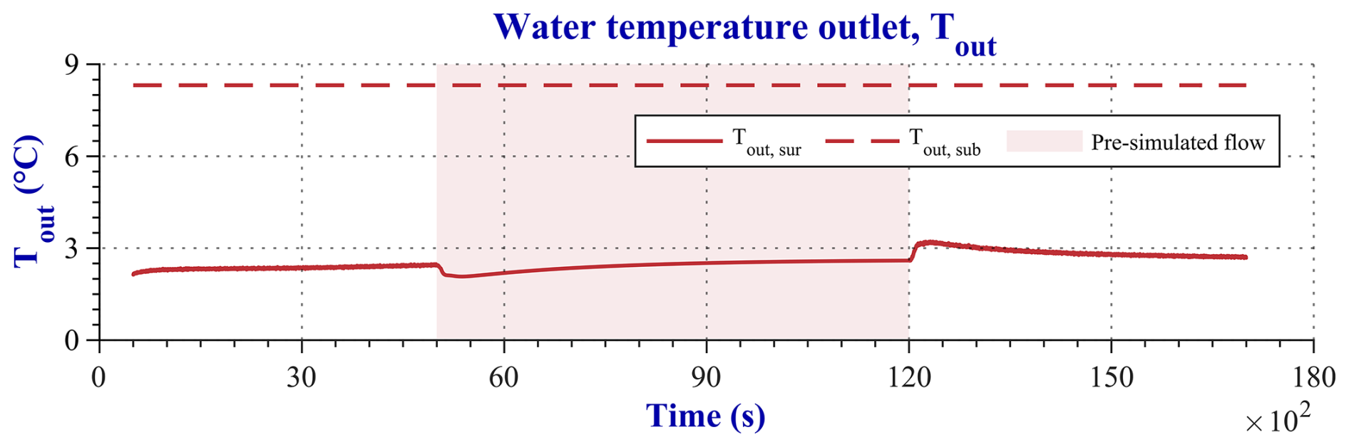
Figure 8 Average water temperature across the surface and subsurface outlet boundaries. The subscripts sur and sub refer to surface and subsurface domains, respectively. The coloured area corresponds to the simulation period in which the pre-simulated flow field was used to only run heat transfer.

4.3 Conservative solute field

The solute analysis skipped the plume caused by the released groundwater and only simulated the mass exchanges that occurred across the river-aquifer interface.

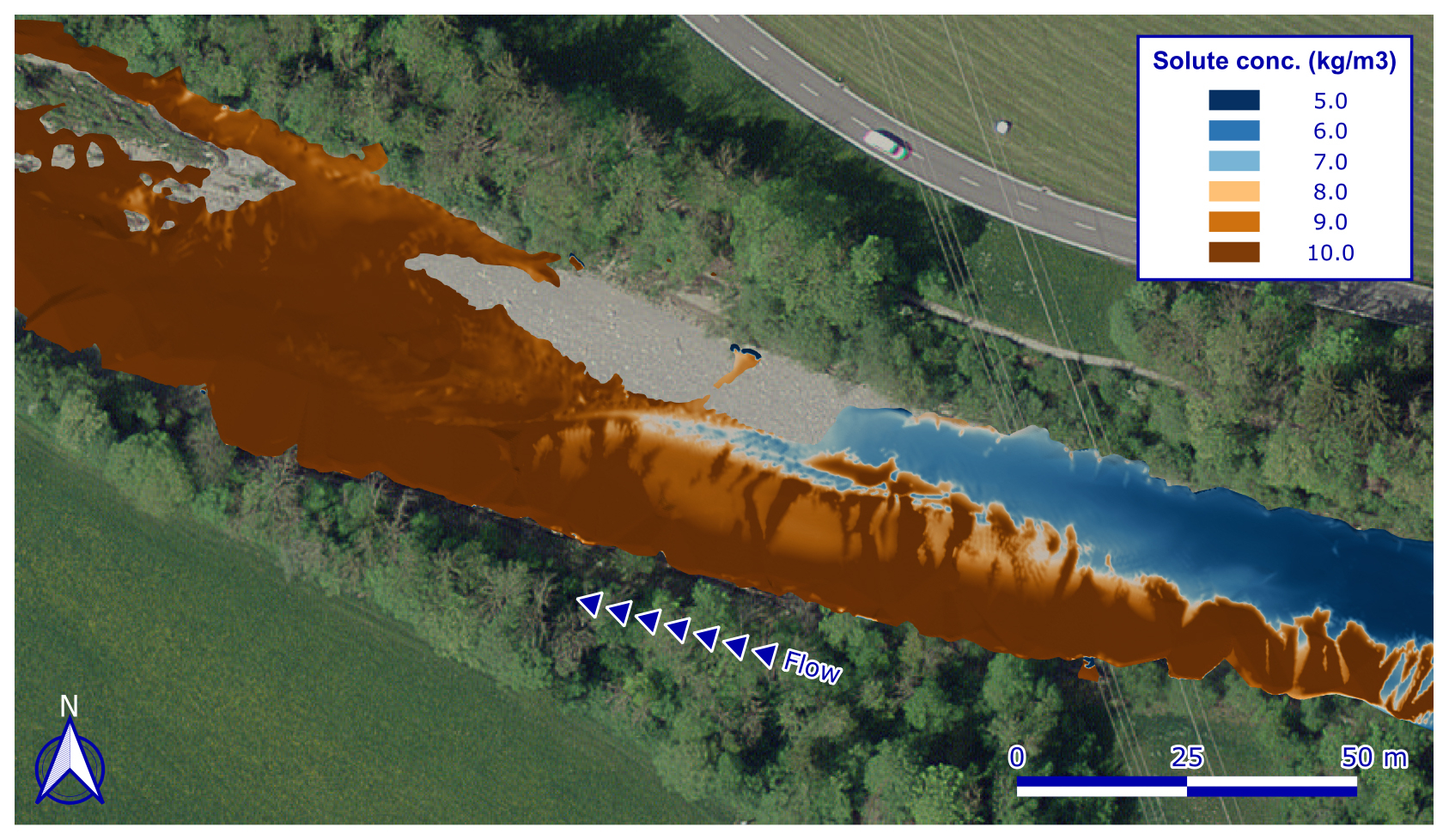
Figure 9 Modelled solute concentration pattern at the riverbed (background image from © Google Maps 2024).

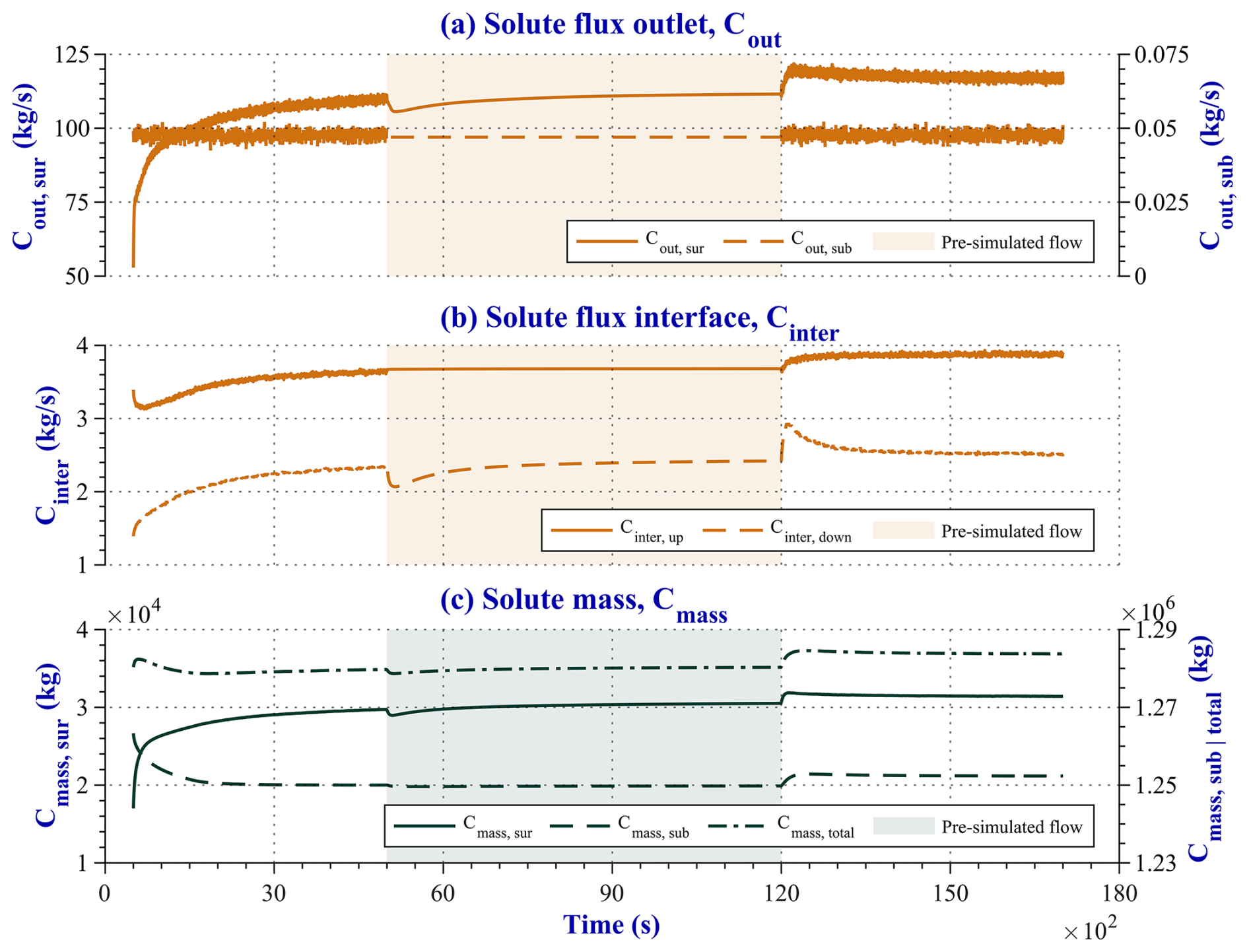
Figure 10 Solute flux across the (a) outlet and (b) interface boundaries. (c) Solute mass in each simulated domain and total mass in the system. The subscripts sur and sub refer to surface and subsurface domains, respectively, while up and down indicate upwelling and downwelling fluxes. The coloured area corresponds to the simulation period in which the pre-simulated flow field was used to only run solute transport.

Initial C_sur,i of 0 and 5 kg m⁻³ were respectively prescribed for the air and water phases, while C_sub,i was initialized to 10 kg m⁻³. Although unrealistic, these high concentration values were chosen to ensure a clear representation of both the interfacial exchanges and the solute mixture in each domain.

The solute concentrations attained at the riverbed are shown in Fig. 9. Analogously to temperature, the bidirectional exchange pattern is mainly located along the shallow channel situated on the left side of the bed. Outside of this zone, no groundwater exfiltration is produced and, thus, the concentrations remain around 5 kg m⁻³. However, in contrast to heat, that diffuses within the surface flow, the solute mass concentrates over time towards the end of the simulation domain. Such accumulation is behind the different extension of subsurface upwelling depicted in Figs. 7a and 9. Yet, the locations where the groundwater actually exfiltrates can be still identified, as they correspond to the darkest spots of the resultant solute field. The pattern described by such spots matches that exhibited by the warm upwelling groundwater, as expected (Fig. 7a).

The aforementioned downstream concentrations are supported by the solute efflux of the surface domain. As plotted in Fig. 10a, the concentration increases over time at the surface outlet while remains essentially stable at its subsurface counterpart. The followed trends confirm the solute accumulation at the surface and also point out the prevalence of subsurface upwelling over surface downwelling. The latter is corroborated by the solute fluxes measured across the riverbed (Fig. 10b), which aligned with the previously described water exchanges (Sect. 4.1).

The solute mass increases in the surface domain and decreases in the subsurface as a result of the described interfacial exchanges (Fig. 10c). The steady-state is reached in both domains once the solute is fully mixed within the system. However, as expected, the total mass is conserved and stays constant throughout the whole simulation. This fact corroborates the system mass balance and, thus, the good functioning of the coupling iterative algorithm at the interface of both domains.

5 Limitations and implications

Analogously to its predecessor, the current version of darcyInterTransportFoam simulates steady-state, fully saturated subsurface flow assuming a static groundwater table. This modelling framework reflects the physical assumption that surface water dynamics occur on timescales much shorter than those governing subsurface flow, thereby justifying the steady-state treatment of groundwater. However, the inability to simulate unsaturated conditions introduces limitations regarding the applicability of the solver. For example, if the groundwater table drops under a clogged streambed, unsaturated zones develop. The code cannot reproduce this disconnection between the surface and the subsurface. Similarly, rapid declines in surface water levels can lead to unsaturated conditions along the riverbanks, which also cannot be represented within the current framework. These limitations are not unique to darcyInterTransportFoam, but were already inherent to hyporheicScalarInterFoam. Nonetheless, scenarios involving localized and well-defined unsaturated regions, such as fine-grained riverbank deposits or seasonally disconnected floodplain margins, can still be approximated with the new code by prescribing impermeable zones and conducting fully-coupled simulations only in the hydraulically connected sections.

Meanwhile, the assumption of full saturation remains valid in other hydrological settings, including gaining river reaches supported by shallow, unconfined aquifers; alluvial valleys with consistently high groundwater tables due to regional discharge; and perennial rivers where sustained baseflow maintains saturation across the riverbed and adjacent banks. For such groundwater systems, Haitjema (2006) developed an approach to assess when steady-state conditions can adequately approximate transient system response to periodic hydraulic stresses. This method calculates an aquifer response time, τ (–), given by:

$$\begin{array}{}\text{(21)}& \mathit{\tau }={\displaystyle \frac{\mathrm{1}}{\mathrm{4}P}}{\displaystyle \frac{S{L}^{\mathrm{2}}}{Kb}},\end{array}$$

where P is the period of the forcing function (365 d for seasonal fluctuations), S is the storativity (specific yield, S_y, for an unconfined aquifer), L is the characteristic system length defined as the distance between major surface water features (m), K is the hydraulic conductivity (m s⁻¹) and b is the saturated thickness (m).

Therefore, prior estimation of τ is recommended to evaluate the suitability of the steady-state groundwater formulation adopted in darcyInterTransportFoam for a given system. In general, small values of τ (τ<0.1) characterize highly permeable unconfined aquifers and most confined aquifers, for which bounding or successive steady-state solutions can be used to represent annual periodicity. Moderately permeable to low-permeability unconfined systems ($\mathrm{0.1}<\mathit{\tau }<\mathrm{1.0}$) are likely to exhibit local transient effects that are not captured by successive steady-state solutions and therefore typically require transient simulations. In low-permeability unconfined aquifers (τ>1.0), the groundwater system responds slowly to periodic changes in recharge or boundary conditions, such that a time-averaged steady-state approximation is appropriate. Further justification for these guidelines is provided in Haitjema (2006) and Anderson et al. (2015).

However, while the current modelling approach may be appropriate for the aforementioned cases, further development of the solver will be required to account for the groundwater table fluctuations and the effects of unsaturated flow on the overall system dynamics. One possible path forward would be to adopt a strategy similar to that implemented in groundwaterFoam (Horgue et al., 2022), which solves unsaturated flow by linearizing the pressure head form of Richards' equation using either Picard's or Newton's method. Additional work will also be needed to develop a reactive solute transport module for the simulation of key biogeochemical reactions (e.g., aerobic respiration, denitrification, etc.). Although previous custom fully-coupled solvers in OpenFOAM, such as hyporheicFoam, were already capable of simulating reactive processes, integrating them into the current framework will require reformulating the module to operate within a two-phase flow context, which adds complexity to its implementation. These enhancements will enable more comprehensive simulations of the dynamic and biogeochemical processes occurring at the river-aquifer interface, even in regions where SW and GW are hydraulically disconnected.

On the other hand, the accessibility to sufficient computational resources to run big CFD models, such as that described in this paper, may represent a limitation to achieving an efficient computation with darcyInterTransportFoam. In this way, the OpenFOAM software allows users to take full advantage of the computer hardware by enabling parallel computations on a theoretically unlimited number of processors. Four mesh decomposition methods are supported to that end. In the present study, the manual decomposition method was applied to ensure an equal division of the surface and subsurface domains. Moreover, 124 CPUs were used to run in parallel the test case on 4 nodes of a local HPC (High-Performance Computing) cluster (2.9 GHz, Ubuntu 22.04.1 LTS operating system). However, access to such amount of computing resources can sometimes be challenging, since most computers are normally equipped with just 8 to 16 cores (with hyperthreading), rarely more. For this reason, it is highly encouraged to use darcyInterTransportFoam on massively parallel machines (e.g. HPC supercomputers or multi-core processors) provided with the necessary computational resources to run any model regardless of its scale and resolution. However, there are some caviates concerning parallelisation. A common recommendation for domain decomposition is that the number of cells hosted per core should lie between 30 000 and 100 000 to guarantee an optimal parallelisation. Whenever this condition is not met and, therefore, the number of cells per core exceeds the recommended cap, the computational times increase dramatically, consequently breaking the compromise between computational efficiency and accuracy in the numerical solution.

Regarding the limitations specific to the simulated test case, the difficulty of acquiring high-resolution in-situ data on the simulated flow, transport and heat processes reduced the availability of field observations for comparison against the model results. The small number of on-site observations (drone-based temperature maps, point temperature measurements and flow data) could initially be considered insufficient to guarantee the quality and accuracy of the simulation. However, the simulated results are consistent with findings from previously conducted field and modelling studies at the site. This agreement, together with the conservation of flow and mass observed in the simulation, provides additional evidence supporting the computational consistency and efficiency of the new solver.

6 Summary and conclusions

An upgraded version of the fully-coupled, three-dimensional SW-GW solver  hyporheicScalarInterFoam, named darcyInterTransportFoam, is presented in this paper. Its novel simulation features are thoroughly described, along with an evaluation of its performance in a test case conducted at a 235 m-long river segment of an actual alluvial aquifer.

The results achieved in the test case confirm the good functioning of the new solver and its add-ons. Such a statement is supported by the facts presented below. The number of the involved solver modification (Sect. 2.3.1) is included between square brackets in each point:

The water flow exits the surface domain freely at a subcritical water height without requiring an obstacle (e.g., a step, ramp or gate) to stabilize the water level before reaching the outlet patch (Bayon-Barrachina and Lopez-Jimenez, 2015) (2).

The parametrization of the real aquifer is captured in the simulated subsurface domain, enabling a realistic estimation of groundwater flowpaths, subsurface velocities and hydraulic heads (1, 3).

Unsaturated regions in the subsurface domain, formed beneath surface dry areas, are no longer a limitation for the computation, as they are defined as impermeable. The simulation is still carried out at the hydraulically connected river-aquifer zones. Accordingly, both direction and length of the flowpaths adjust to the physical and geological characteristics of the system (1, 3).

Passive solute transport and heat transfer are effectively simulated in the surface and subsurface domains. Additionally, both processes are solved in a single phase (water) in the surface domain. The agreement between the modelled outcomes and field observations further validates this model's performance (4, 5, 6, 8).

Both water and solute mass balances are conserved within the system, which ensures the flux consistency across the interface of both domains (1, 5, 7, 8).

Water, solute and temperature results exhibit interconnected behaviour. Similarly, the flux exchanges across the interface and the mass balance of each domain display interdependent dynamics (1, 4, 5, 6, 7, 8).

The above points illustrate that, despite the modelling limitations of the present version of darcyInterTransportFoam, the new solver fills most of the simulation gaps of its predecessor, hyporheicScalarInterFoam. In this way, the model is successfully applied to solve the flow, solute and heat exchanges across the riverbed of the selected Emme River segment. Moreover, its utility to study the SW-GW interactions and dynamics beyond the hyporheic zone is also demonstrated through its application to a reach-scale scenario.

The successful performance of darcyInterTransportFoam confirms its potential for simulating multiple hydrogeological scenarios, underpinned by its capability to represent the intricate characteristics of natural systems and the diverse dynamic processes they drive. Among its new functionalities, the ability to prescribe heterogeneity and anisotropy in the subsurface, as well as to define layers or anthropogenic structures (e.g., weirs), represents a significant step toward more physically realistic riverbed-aquifer interactions. This feature, combined with the solute transport and heat transfer modelling, enables the simulation of important feedback mechanisms between SW and GW, whose detailed dynamics could not be accounted for in the previous version of the solver. For instance, the migration of a contaminant plume from GW into a river under geologically complex conditions can now be simulated, with spatial variability in K_ij and θ_i governing both the transport pathways and the timing of pollutant discharge. Similarly, the inclusion of stratified layering and anisotropic properties allows for a more accurate representation of gaining-losing conditions and hyporheic exchanges, both of which are highly sensitive to subsurface characterization and drive key biogeochemical processes. In such contexts, temperature dynamics act not only as tracers but also as active drivers of biochemical reactions. Moreover, in river-aquifer systems affected by anthropogenic modifications, such as dams, levees or bank reinforcements, the improved modelling framework enables the explicit definition of these structures to assess their influence on hydraulic connectivity, and consequently on processes like solute retention and thermal buffering.

Further code development is still needed to address the remaining limitations of the current solver version, such as the simulation of unsaturated flow and multicomponent reactive transport. Closing these gaps will enable a more comprehensive representation of the physical and biogeochemical processes occurring at the river–aquifer interface.

Appendix A

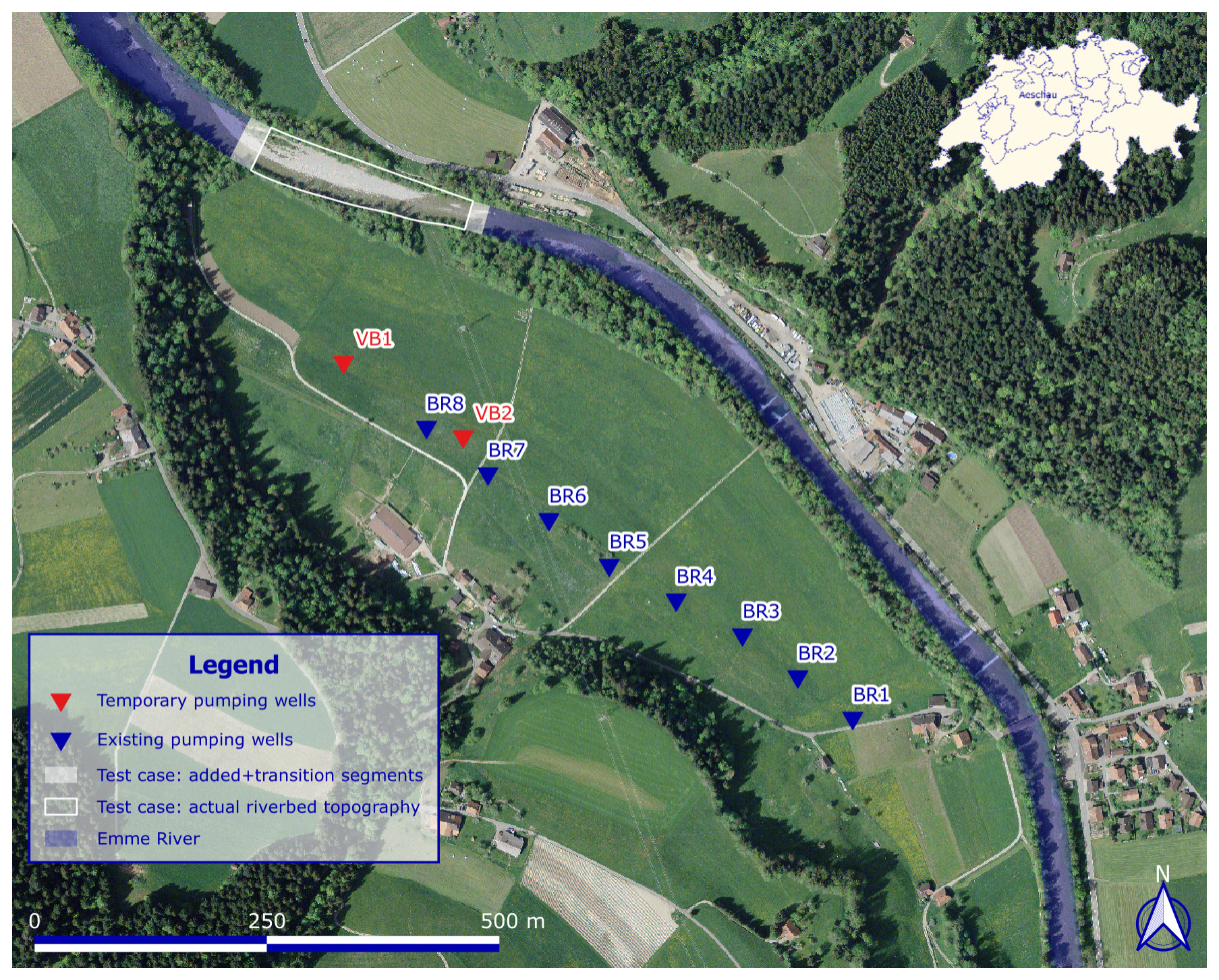
Figure A1 Location of the model's test case in the Emme River (background image from © Google Maps 2024).

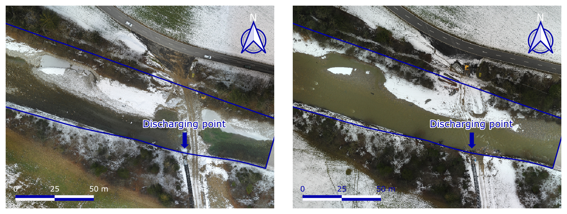
Figure A2 Snapshot of the pipes releasing pumped groundwater in the Emme River at two different flow scenarios (background image captured on site by the drone).

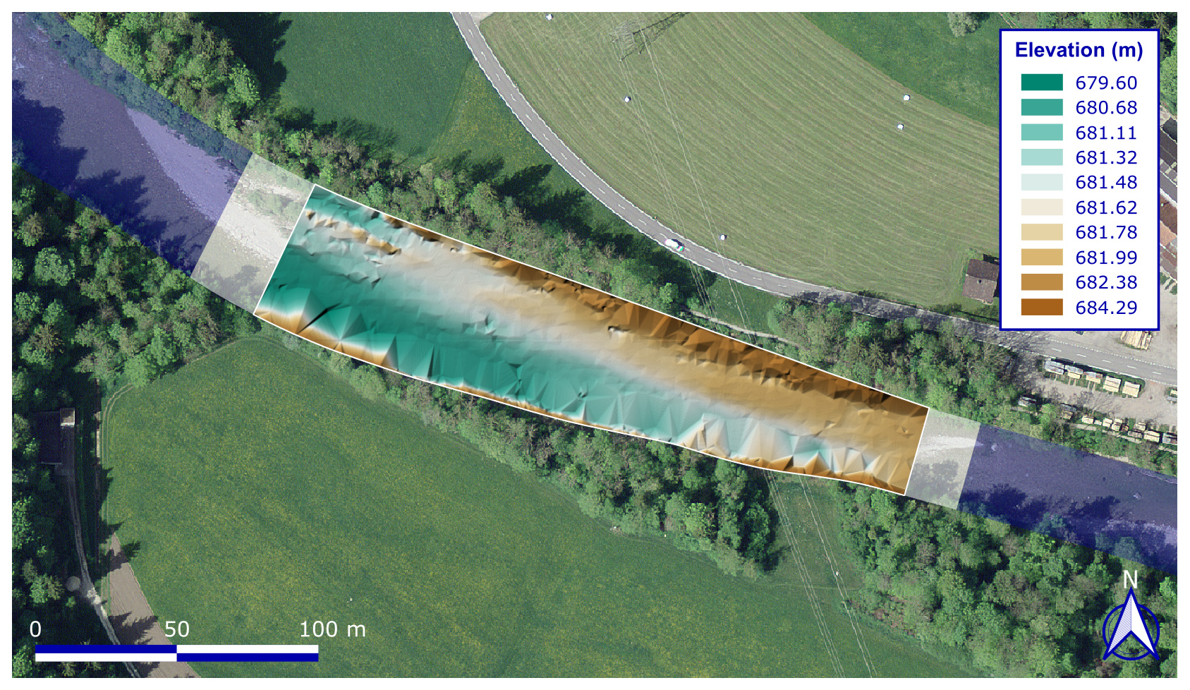
Figure A3 High-resolution (25 cm) riverbed DEM used to define the 3D meshes of the test case (background image from © Google Maps 2024).

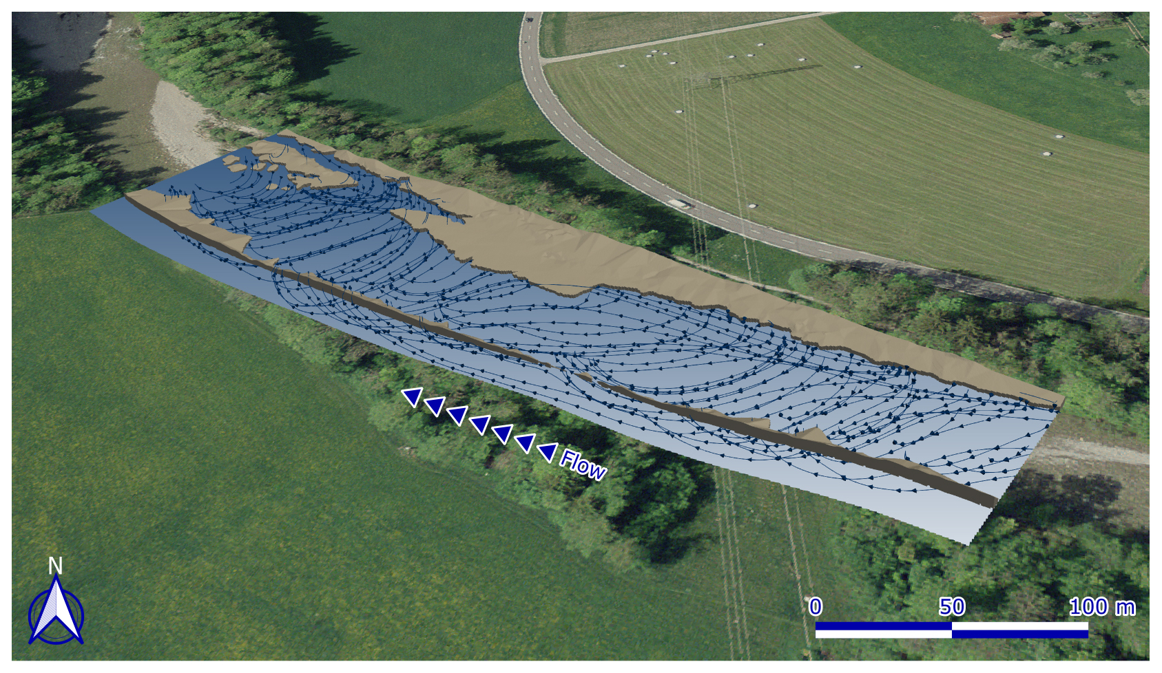
Figure A4 3D view of the simulated groundwater flowpaths underneath the riverbed (background image from © Google Maps 2024).

Table A1 Surface and subsurface (italic) fluid and geological parameters defined in the test case.

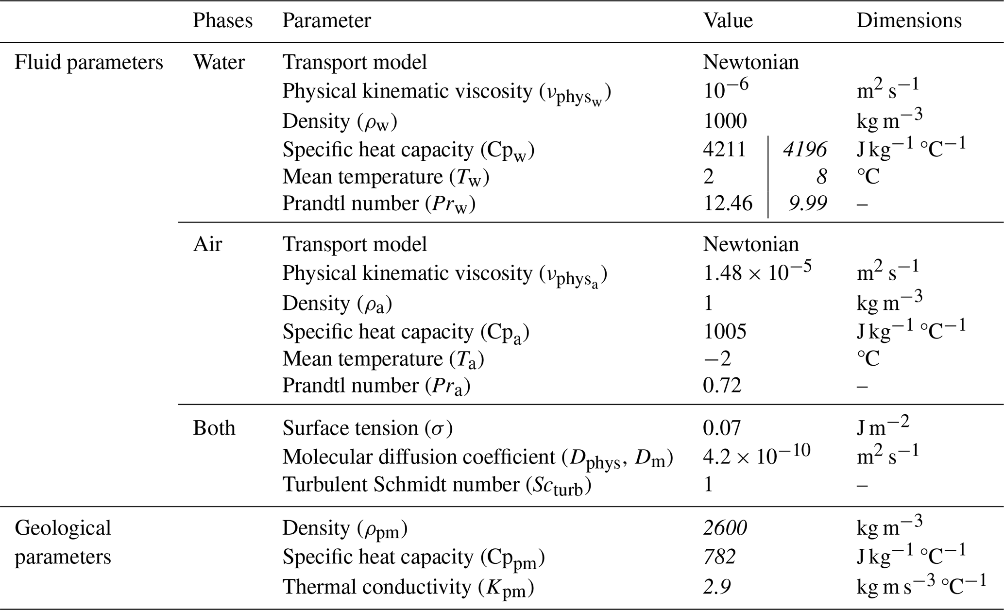
Table A2 Initial (IC) and boundary conditions (BC) defined for each surface variable.

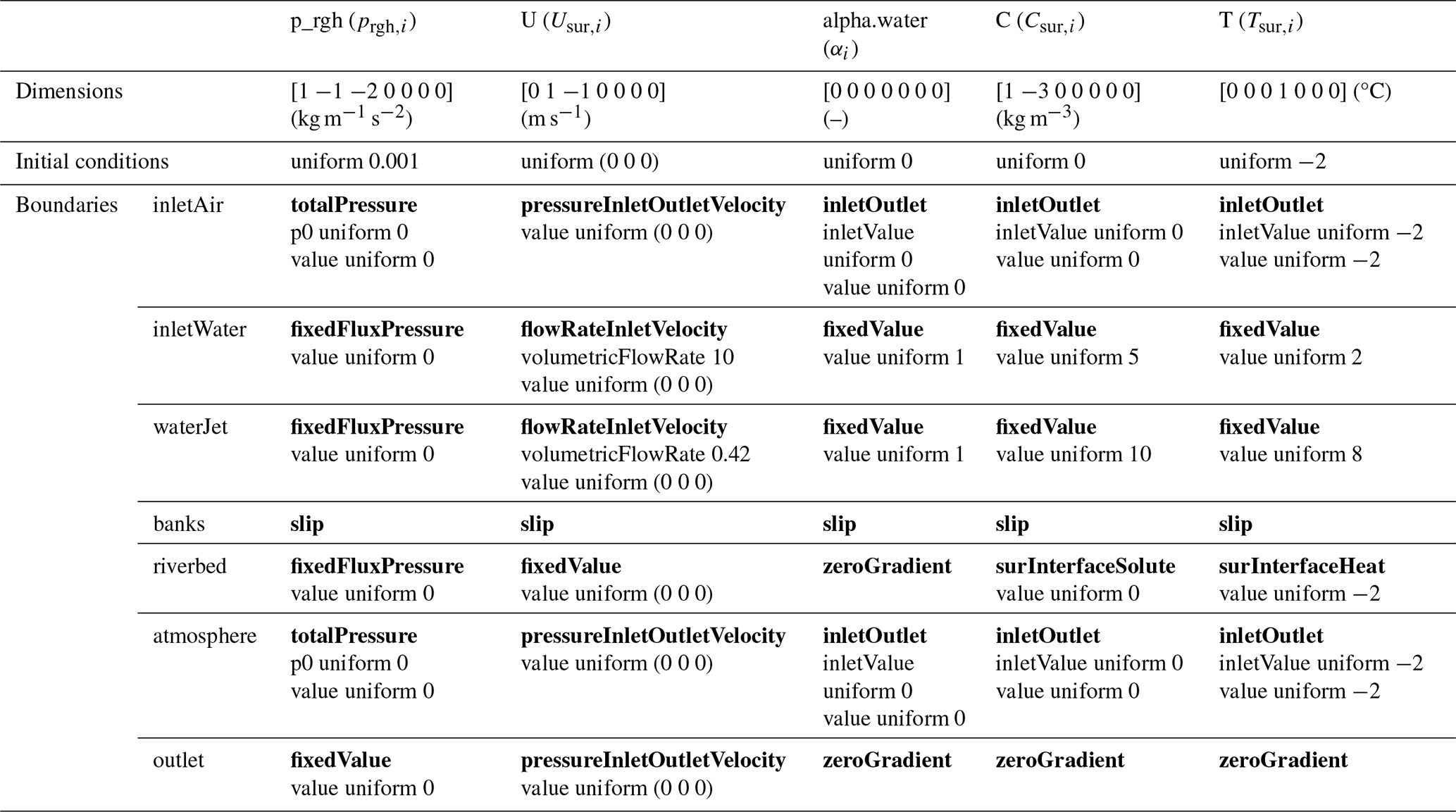
Table A3 Initial (IC) and boundary conditions (BC) defined for each kOmegaSST turbulence model variable.

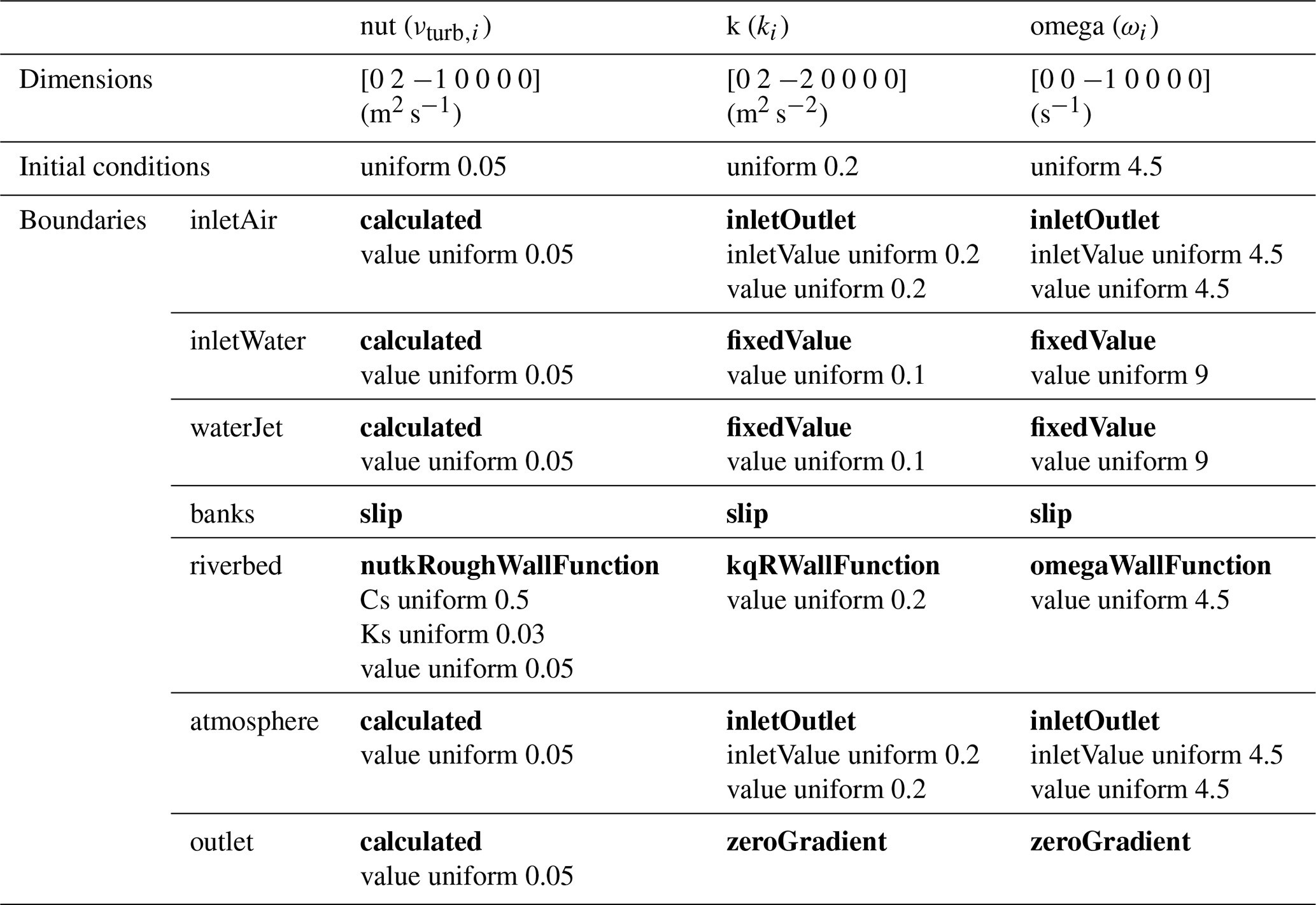
Table A4 Initial (IC) and boundary conditions (BC) defined for each subsurface variable.

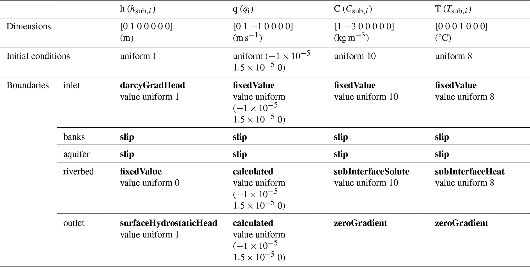
Table A5 Numerical schemes selected to discretize the surface and subsurface equation terms.

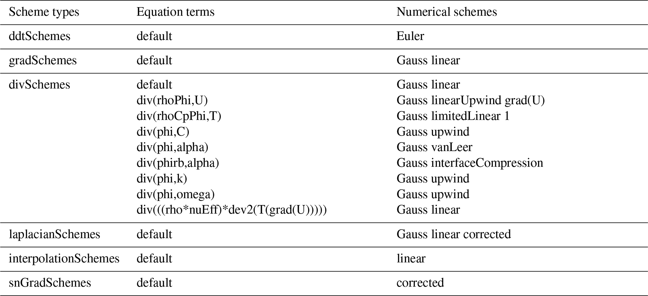
Table A6 Numerical solvers selected to solve the surface and subsurface (italic) variables.