Benchmarking soil moisture and its relationship to ecohydrologic variables in Earth System Models

Soil moisture (SM) is a key regulator of ecosystem biogeophysics, influencing plant water relations and land-atmosphere energy exchanges. We evaluate the representation of SM in 16 Earth System Models from the Coupled Model Intercomparison Project Phase 6 (CMIP6) using the International Land Model Benchmarking (ILAMB) framework, focusing on surface (0–5, 0–10 cm) and rootzone (0–100 cm) depths, as well as key ecohydrological variables like gross primary productivity (GPP), leaf area index (LAI), and evapotranspiration (ET), and their coupling. Models are benchmarked against multiple observational and assimilated datasets to assess both state variables and cross-variable relationships. Surface SM is generally well represented (r > 0.87), while rootzone SM variability is systematically overestimated (normalized standard deviation > 1). ET shows strong agreement with observations (r > 0.9), whereas GPP and LAI exhibit larger inter-model spread. Skill in individual variables does not guarantee realistic SM–ecohydrology coupling, which varies strongly across models and depends on the reference dataset. Köppen-based regional analyses reveal strong regime dependence, with several models performing well in Tropical and Temperate regions but degrading in Continental (high-latitude) zones. Across both global and regional benchmarks, models cluster by land surface framework, indicating that structural choices in soil hydrology and soil–plant coupling exert a first-order control on performance. These results provide process-relevant benchmarks and suggest that improving the representation of vertical soil structure, rooting depth distributions, and soil–plant hydraulic coupling will be central to advancing soil moisture realism in next-generation Earth system models.

1 Introduction

Soil moisture (SM) plays a central role in regulating Earth system processes by controlling the storage and exchange of water, carbon, and energy between the land surface and atmosphere (Clark et al., 2015; Trugman et al., 2018; Green et al., 2019; Massoud et al., 2020). Accurately representing SM in Earth System Models (ESMs) is essential for improving predictions of the Earth system (Seneviratne et al., 2010; Hauser et al., 2016; Humphrey et al., 2021). ESMs simulate these processes through coupled biogeochemical and hydrological cycles, both of which are strongly influenced by SM. However, accurately modeling SM at ESM grid scales remains challenging due to heterogeneity in soil properties, scale mismatches between physical processes and model resolution, and limited knowledge of subsurface boundary conditions (e.g., groundwater depth). As a result, ESMs adopt a range of approaches to simulate SM. The majority rely on “bucket-type” models that route water through discrete soil layers using threshold-based parameters (e.g., field capacity) and rate-dependent functions (e.g., hydraulic conductivity).

This work seeks to evaluate the representation of SM in ESMs by using the International Land Model Benchmarking (ILAMB) framework (Collier et al., 2018), a tool extensively used to assess the performance of land models. ILAMB provides a standardized, reproducible evaluation framework that compares model output against observational benchmarks using a suite of complementary metrics, including measures of bias, variability, seasonal cycle, and spatial pattern agreement. Its modular design and consistent scoring methodology make it well suited for systematic, multi-model intercomparison and for diagnosing strengths and weaknesses across different components of the land surface system. Although ILAMB has been applied to various ecohydrologic processes and properties such as gross primary production (GPP) (Caen et al., 2022), evapotranspiration (ET) (Wu et al., 2020), and leaf area index (LAI) (Yang et al., 2023), SM has remained mostly underrepresented in ILAMB-based model evaluations until now.

Despite advances in ESMs, the accurate simulation of SM in Coupled Model Intercomparison Project Phase 6 (CMIP6) remains a persistent challenge due to structural biases and uncertainties in land surface processes. Several studies have highlighted both improvements and limitations in how CMIP6 models represent SM. For example, Yuan et al. (2021) showed that CMIP6 models better capture historical surface SM trends over the contiguous United States (CONUS) compared to CMIP5, particularly in regions like the Northwest and Midwest. However, considerable inter-model variability remains, suggesting a need for further refinement in future model generations. Similarly, Wang et al. (2022) conducted a comprehensive evaluation of CMIP6 SM simulations over China and found that while the multi-model mean (MME) generally captured observed spatial patterns and seasonal cycles of both near-surface and rootzone SM, substantial inter-model spread persisted, particularly in trends and interannual variability. Their findings also emphasized the dominant role of land surface schemes in driving model behavior, as models developed by the same institution often exhibited similar performance. Moreover, Purdy et al. (2018) illustrated the potential for significant improvement in model performance through better SM representation, showing that integrating SM information from satellite data into model simulations reduced global ET errors by up to 23 % in dry regions. These studies point to the critical need to identify and correct structural biases that limit current model skill in simulating SM.

At the same time, the importance of accurately simulating SM extends beyond model performance metrics. Zuo et al. (2024) highlighted that maintaining current global SM levels could reduce nearly a third of projected land warming under low-emission scenarios. Their results, based on outputs from historical CMIP6 experiments and other model intercomparison projects, highlight the central role SM plays in climate feedbacks and the reliance on models like CMIP6 to inform future projections. Given both the challenges and stakes involved, this study benchmarks SM and its coupling with ecohydrologic processes such as GPP, LAI, and ET, with the goal of identifying model limitations and guiding improvements as we look toward CMIP7 and beyond.

The evaluation of SM in global models has a long history, with early efforts dating back to Robock et al. (1998) as part of the Atmospheric Model Intercomparison Project (AMIP). In their analysis, they found significant discrepancies in how SM was represented and simulated across different models, an issue that was prominent 25 years ago and remains a challenge today. More recently, Qiao et al. (2022) conducted a detailed evaluation of SM using a suite of CMIP6 models, examining both surface and deeper SM (up to 2 m) across various subregions around the globe. They found that the multimodel ensemble mean generally produces reasonable representations for overall climatology. However, their study relied on reanalysis products and data assimilation systems as the reference for benchmarking (Qiao et al., 2022), which, while widely used, are not true SM observational products but rather model-based estimates. Furthermore, Qiao et al. (2022) assumed that the model outputs mrsos (surface SM) and mrsol (layered SM) represent the same variable, despite their structural differences (Massoud et al., 2026). In reality, mrsol provides moisture values at multiple soil layers, from which mrsos, representing moisture in the top 10 cm of soil, is derived. Other studies used a combination of observation and model-based benchmarks, but are limited to regional domains and similarly do not distinguish the different nature of mrsos and mrsol (Yuan et al., 2021; Wang et al., 2022). In this current study, we distinguish between these two variables and apply depth-specific derivations to more accurately evaluate SM representation across different layers in the models. Here, we not only benchmark SM at various depths, but also evaluate key ecohydrologic variables such as GPP, LAI, and ET, both individually and in relation to SM, to provide a more comprehensive assessment of land surface processes in CMIP6 models.

One of the persistent challenges in benchmarking SM is the limited availability of high-quality datasets. To address this, we utilize two key datasets for global-scale benchmarking in this study. The first is the Wang et al. (2021) product, which is a weighted average of multiple sources, including offline land surface model simulations, remote sensing data, and reanalysis products, that was found to outperform the original sources in that study. This dataset provides estimates for both surface SM (top 10 cm) and rootzone SM (up to 1 m), offering a view of SM at different depths. The second dataset is the European Space Agency Climate Change Initiative SM (ESA-CCI SM) product (Dorigo et al., 2015, 2017; Gruber et al., 2019; Preimesberger et al., 2021, 2025), which is derived from a blend of passive and active satellite sensors. ESA-CCI SM represents surface SM down to 5 cm, and its combination of different satellite platforms helps mitigate the limitations of individual sensors, providing an observational estimate for surface SM that is robust. Together, these datasets allow for a more thorough evaluation of SM in CMIP6 models. We emphasize that neither of these products represents a definitive “truth,” as both incorporate model-based information and are subject to their own structural assumptions and uncertainties. In contrast to studies that rely on a single reanalysis-based reference (e.g., Qiao et al., 2022), our approach intentionally combines complementary datasets with differing methodologies, including satellite-based observations (ESA-CCI) and a blended product integrating offline models, reanalysis, and satellite constraints (Wang et al., 2021). By using multiple reference products rather than a single benchmark, our goal is to provide a more robust and balanced assessment of model performance and to reduce reliance on any one dataset. We note that soil moisture below 1 m can also be important for ecosystem functioning (Stocker et al., 2023), particularly in regions with deep rooting systems (Kühnhammer et al., 2023), but evaluating deeper soil layers is beyond the scope of this study and we therefore focus on surface and rootzone soil moisture.

While benchmarking SM alone can offer insights into model performance, understanding how SM interacts with other ecosystem processes such as GPP, ET, and LAI can yield additional clues into the strengths and weaknesses of these models (Guswa et al., 2002; Wang et al., 2019). By examining how models' skills are related to certain model processes, we aim to uncover patterns that point to specific model limitations, whether they stem from structural design, input data, or parameterizations. Ultimately, this work seeks to guide improvements in model development and reduce uncertainties in global SM simulations. The goals of this study are threefold. First, we benchmark CMIP6 models in their simulation of SM at multiple depths, specifically at 5, 10, and 100 cm, using various datasets. Second, we assess model performance in simulating key ecohydrologic variables, including GPP, LAI, ET, as well as the relationships between SM and each of these variables. Third, we aim to identify specific areas for improvement, whether in individual models or as systematic issues across the CMIP6 ensemble. To support these objectives, we also implement a Köppen climate region analysis (Peel et al., 2007) within the ILAMB framework to evaluate model performance across distinct climate zones.

2 Materials and Methods

2.1 Models and Variables in CMIP6 Simulations

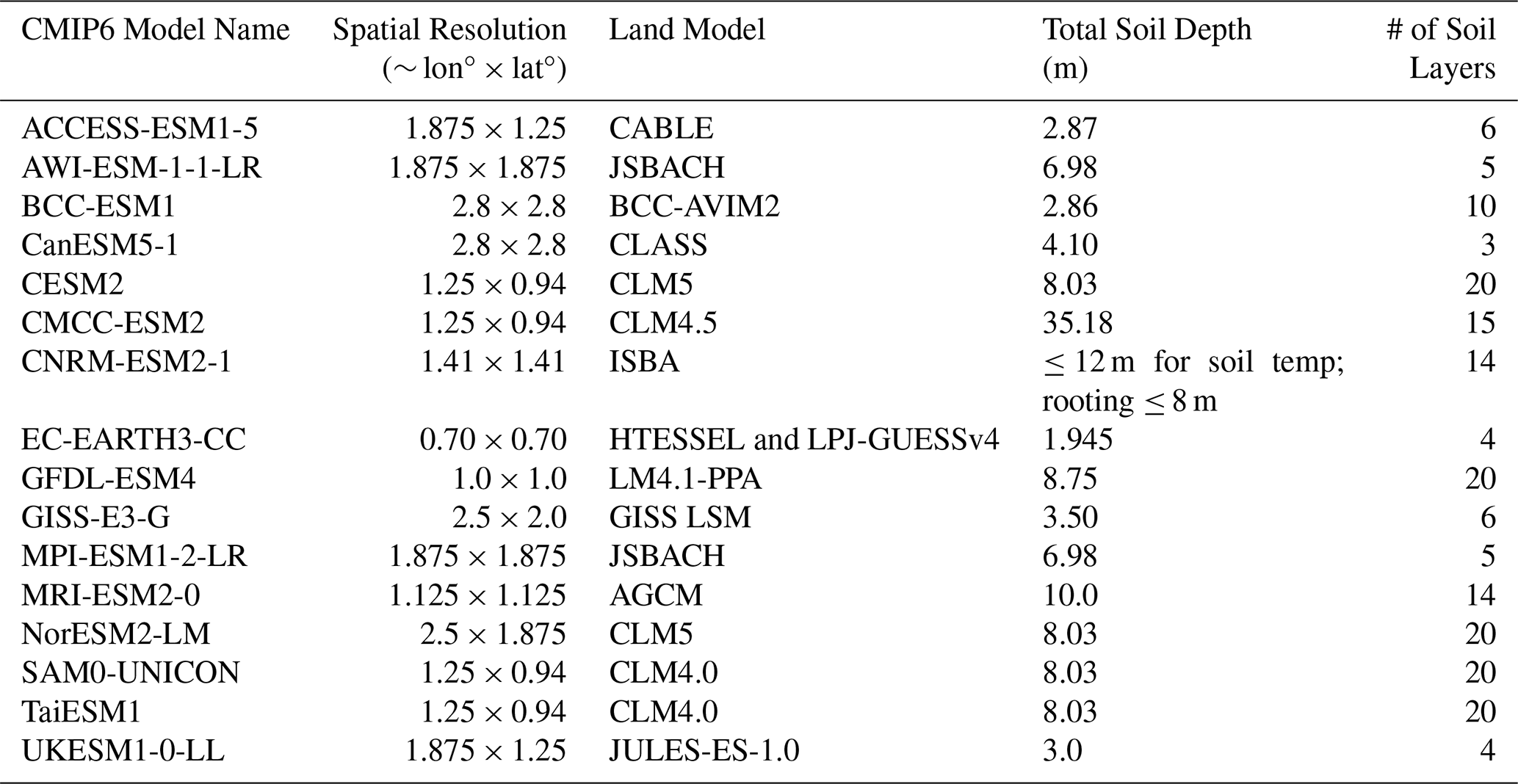
The model data used in this study come from CMIP6 (Eyring et al., 2016), an international effort to standardize ESM simulations, enabling direct comparison across models. We use a suite of CMIP6 models (detailed in Table 1) that differ in their spatial resolutions and land surface model components. Table 1 lists each model's horizontal grid spacing and the land surface scheme used to simulate SM, GPP, LAI, and ET.

The SM variables analyzed are mrsol and mrsos, which represent layered and surface soil moisture, respectively. Both variables are provided in units of mass per unit area [kg m⁻²]. Other simulated variables include gpp (units g m² d⁻¹), lai (unitless), and evspsbl (units mm d⁻¹) corresponding to GPP, LAI, and ET. All variables are analyzed at monthly temporal resolution.

To derive SM at specific depths (e.g., 0–5, 0–10, or 0–100 cm), we calculate depth-integrated soil moisture estimates from the mrsol variable, which provides total SM contained in each discrete model soil layer. Since the vertical layering varies across models, we apply a depth-weighted integration approach that also converts units from mass to volumetric SM (i.e., from [kg m⁻²] to [m³ m⁻³]). This conversion and integration is expressed as:

$$\begin{array}{}\text{(1)}& \begin{array}{rl}{\mathrm{SM}}_{\mathrm{integrated}}& =\left\{\left[{\sum }_{\mathrm{layer}i=\mathrm{1}}^{\mathrm{layer}n-\mathrm{1}}{\displaystyle \frac{\mathrm{mrsol}\left(i\right)}{{\mathit{\rho }}_{\mathrm{w}}\cdot \mathrm{d}z\left(i\right)}}\cdot \mathrm{d}z\left(i\right)\right]\right.\\ & \left.+\left[{\displaystyle \frac{\mathrm{mrsol}\left(n\right)}{{\mathit{\rho }}_{\mathrm{w}}\cdot \mathrm{d}z\left(i\right)}}\cdot z_{\mathrm{remaining}}\right]\right\}/z_{\mathrm{total}}\end{array}\end{array}$$

In this equation, mrsol(i) represents the mass of SM in the ith model-defined soil layer, reported in units of [kg m⁻²]. The variable ρ_w is the density of liquid water, assumed to be a constant value of 1000 kg m⁻³. The quantity dz(i) refers to the thickness of the ith soil layer in meters [m], which is used to compute the volumetric contribution of each layer. The term z_remaining represents the portion in [m] of the final layer that partially overlaps with the target integration depth (e.g., if the target is 10 cm and the final layer spans from 8–15 cm, then z_remaining=2 cm = 0.02 m. The total integration depth, z_total, is the sum of all full-layer thicknesses plus z_remaining, defining the vertical extent over which SM is integrated.

This formula first converts each layer's SM from mass per unit area [kg m⁻²] to volumetric SM [m³ m⁻³] by dividing by the product of water density and layer thickness. Then, it multiplies by the layer thickness to compute the volume per unit area. Summing over all layers and dividing by the total soil depth yields the average volumetric SM over the target depth. This method standardizes SM across models with differing vertical discretizations and unit conventions, enabling accurate and consistent comparisons with benchmarking datasets, which report SM as a volume fraction. For surface SM (mrsos), which represents a shallow fixed-depth layer (i.e., 0.1 m), we apply the same conversion logic by assuming that fixed depth during volumetric transformation. This approach is consistent with prior studies (e.g., Qiao et al., 2022; Wang et al., 2022; Massoud et al., 2026).

Table 1 CMIP6 models used in this study, along with their latitude and longitude grid sizes and the land models with their soil depths and number of soil layers used in each model.

2.2 Soil Moisture Datasets Used for Benchmarking

In this study, we evaluate the SM performance of CMIP6 models using two primary benchmark datasets. The first is the ESA-CCI SM product (Dorigo et al., 2017; Gruber et al., 2019; Preimesberger et al., 2021), which provides a global, long-term record of surface SM (∼ 2–5 cm) spanning over 40 years (1978–2023) at a daily temporal resolution that is aggregated to reflect monthly values and spatial resolution of approximately 25 km (Fig. 1A). The ESA-CCI SM product is updated annually through an algorithmic process that incorporates data from both passive and active satellite sensors, producing a blended dataset that integrates multiple sensor sources while extending the time series with each update. This dataset has been extensively used in hydrological and climatological research (e.g., An et al., 2016; McNally et al., 2016; Ciabatta et al., 2018; Massoud et al., 2023; Li et al., 2025a), including the Bulletin of the American Meteorological Society's annual “State of the Climate” reports. Its long-term, global coverage makes it a valuable resource for evaluating surface SM in ESMs. To facilitate direct comparison with the ESA-CCI SM product that typically represents SM at a depth of 5 cm, the mrsol variable in each CMIP6 model is integrated to the 5 cm layer using Eq. (1). Given that some models have first layers that are deeper than 5 cm, this integration may introduce additional uncertainty in the estimated SM.

The second SM dataset used in this study is the Wang et al. (2021) product, which provides a global, gap-free, long-term record of SM across four depths (0–10, 10–30, 30–50, and 50–100 cm) from 1970 to 2016, with a monthly temporal resolution and spatial resolution of 0.5°. This dataset synthesizes SM information from diverse sources, including in situ observations, satellite data, reanalysis products, and offline land surface model simulations. It employs three statistical approaches, unweighted averaging, optimal linear combination (OLC), and emergent constraint (EC), to produce a merged product that outperforms individual source datasets in terms of bias, root mean square error (RMSE), and correlation when compared to in situ observations. For this study, we utilize the OLC version of the Wang et al. (2021) product, which we hereafter refer to as Wang2021OLC, because it is constrained by in situ observational values and performs among the best of the paper's reported method-data source combinations. This hybrid dataset offers harmonized spatial, temporal, and vertical coverage, making it highly suitable for large-scale ESM benchmarking of both surface (Fig. 1B) and rootzone (Fig. 1C) SM. Since this dataset provides SM estimates at both 10 and 100 cm depths, we integrate the mrsol variable from each CMIP6 model to these depths using Eq. (1) to enable direct comparison. In addition, because the mrsos variable in CMIP6 models also represents surface SM at approximately 10 cm, it is separately benchmarked against the 10 cm layer from the Wang2021OLC product. This dual use of mrsol and mrsos allows us to assess the internal consistency and depth representation of SM across different model variables and observational references.

While these datasets are widely used and provide valuable long-term, global-scale estimates, each has inherent limitations, including retrieval uncertainties, differences in spatial and temporal resolution, and dependence on model-based or algorithmic assumptions. Because no single dataset can fully capture the complexity of SM dynamics, the use of multiple, complementary observational and assimilated products helps quantify uncertainty in the benchmark results presented here.

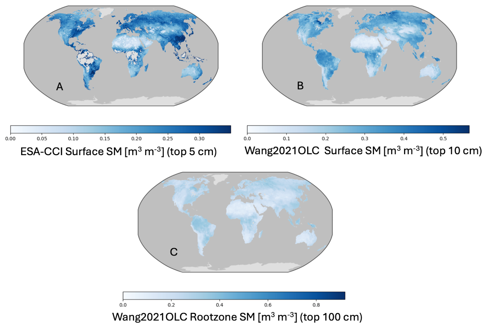
Figure 1 Long-term mean soil moisture (SM) from observational datasets. (A) ESA-CCI Surface SM [m³ m⁻³] (top 5 cm) (1978–2023), providing global estimates based on satellite data. (B) Wang et al. (2021) OLC Surface SM [m³ m⁻³] (top 10 cm) (1970–2016), derived from a merged dataset of satellite and in-situ observations. (C) Wang et al. (2021) OLC Rootzone SM [m³ m⁻³] (top 100 cm), representing long-term mean soil moisture across the rootzone. Each subplot shows the global distribution of soil moisture at the depths represented in each product.

2.3 Other Benchmark Datasets

For the ecohydrologic relationship variables, we incorporate observational datasets specific to each variable that exist in the ILAMB data library. GPP observations are derived from the Water, Energy, and Carbon with Artificial Neural Networks (WECANN) dataset, which provides globally gridded estimates based on advanced machine learning approaches that integrate remote sensing and meteorological inputs (Alemohammad et al., 2017) from 2007 to 2016. LAI data is sourced from the NOAA Climate Data Record (CDR) of AVHRR Leaf Area Index (AVH15C1) from 1981 to 2019 (Claverie et al., 2016). ET data comes from the Global Land Evaporation Amsterdam Model (GLEAM) v3.3a, which provides daily estimates (aggregated here to reflect monthly values) from 1980 to 2018 (Miralles et al., 2011; Martens et al., 2017). The spatial resolution of the WECANN GPP product (Fig. 2A) is 0.5°, that of the AVH15C1 LAI data (Fig. 2B) is 0.05°, and that of the GLEAMv3.3a ET data (Fig. 2C) is 0.25°.

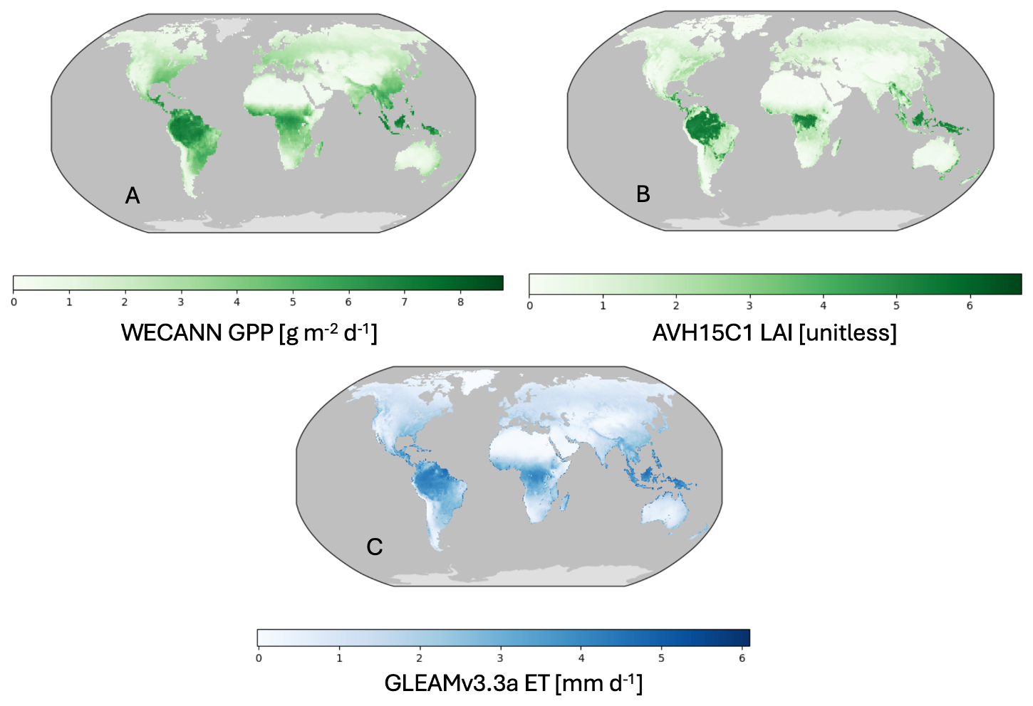
Figure 2 Long-term mean ecohydrological variables from observational datasets. (A) WECANN GPP [g m⁻² d⁻¹ ] (2007–2016), providing global estimates of gross primary productivity derived from machine learning techniques. (B) AVH15C1 LAI [unitless] (1981–2019), representing global leaf area index values from the NOAA Climate Data Record. (C) GLEAMv3.3a ET [mm d⁻¹] (1980–2018), showing global evapotranspiration estimates derived from satellite observations and meteorological data. Each subplot displays the global distribution of these ecohydrological variables.

While ILAMB supports multiple observational datasets for each variable, we utilize a single benchmark dataset per variable in this study to maintain consistency and simplicity in our analysis. GPP observations are taken from the WECANN product (Alemohammad et al., 2017), which provides globally gridded estimates derived from machine-learning approaches that integrate satellite and meteorological data. LAI is evaluated using the NOAA Climate Data Record AVH15C1 product (Claverie et al., 2016; NOAA CDR AVH15C1), which offers a long-term, internally consistent record based on AVHRR observations. ET is benchmarked against GLEAM v3.3a (Miralles et al., 2011; Martens et al., 2017), a widely used dataset that combines satellite observations with a physically based modeling framework.

It is worth noting that although these products are widely used as observational references, they are themselves derived from models or statistical algorithms informed by observational inputs, and therefore should be interpreted as observationally informed estimates rather than direct measurements. Each dataset also carries known limitations, including uncertainties related to retrieval algorithms, input data quality, and assumptions embedded in the underlying models. Nonetheless, these datasets have been extensively evaluated and applied in previous studies and provide reliable and widely accepted benchmarks for evaluating modeled GPP, LAI, and ET (represented by the gpp, lai, and evspsbl variables), supporting a comprehensive evaluation of ecohydrologic processes and their relationships with SM.

2.4 ILAMB Framework

The ILAMB framework is an open-source software package used to assess the performance of ESMs by comparing model outputs to a suite of observational datasets. ILAMB's scoring system integrates several key performance metrics: bias, RMSE, seasonal cycle representation, and spatial distribution (Fig. A1). These metrics are synthesized into an overall score using the method detailed in Collier et al. (2018), offering a quantitative view of model fidelity. Bias measures the average deviation from observational data, RMSE quantifies error magnitude, and the seasonal cycle and spatial metrics assess the temporal and geographic accuracy of model outputs. By combining these metrics, ILAMB generates diagnostic graphics and scores to help identify strengths and weaknesses in model simulations. The ILAMB framework has been widely adopted for model evaluation and intercomparison, aiding in the continuous development of more accurate land model components (Collier et al., 2018, 2023).

In this study, we extend the ILAMB analysis by incorporating Köppen climate classifications, which allows for a more detailed evaluation of model performance across diverse climate zones. These regions, which include tropical, desert and semi-arid, temperate, and continental climates, reflect varying environmental conditions that significantly influence SM and vegetation dynamics. By examining model skill within these distinct climate zones, we gain deeper insights into region-specific strengths and weaknesses, allowing for targeted improvements in land models across climate types.

3 Results from ILAMB

3.1 Overall benchmark scores in ILAMB

In this section, we summarize the global performance of CMIP6 models using the ILAMB framework across surface and rootzone soil moisture (SM) and key ecohydrological variables. The combined results are shown in the ILAMB portrait plot (Fig. 3), where colors indicate relative performance across models and metrics, with purple denoting higher skill and orange lower skill. The Overall Score is a composite metric that combines normalized measures of bias, error magnitude (RMSE), seasonal cycle representation, and spatial pattern agreement following the ILAMB methodology (Collier et al., 2018). The Seasonal Cycle Score evaluates how well models capture the timing and amplitude of the observed annual cycle, while the Spatial Distribution Score measures agreement in spatial patterns across grid cells.

Rather than showing uniform behavior across variables, the models exhibit distinct and structured performance patterns. Some models display relatively strong skill for ecohydrological variables (GPP, LAI, and ET) but weaker performance for soil moisture itself, while others perform well for soil moisture states but less well for vegetation and flux variables. As a result, the coupling metrics between SM and ecohydrological variables often differ markedly from the skill in the individual variables alone. This indicates that reproducing realistic mean states or variability does not necessarily imply that models capture the correct sensitivity of ecosystem processes to soil moisture.

Notably, models based on the same land surface framework tend to exhibit similar performance signatures (e.g., CESM2 and NorESM2-LM using CLM5, and MPI-ESM1-2-LR and AWI-ESM-1-1-LR using JSBACH; see Table A1). This structural coherence suggests that differences in land model formulation play an important role in shaping benchmarking outcomes, motivating a more detailed examination of soil moisture, ecohydrological variables, and their coupling in the following subsections. We note that comparable process-level documentation is not always consistently available across all CMIP6 models; therefore, Table A1 summarizes key characteristics only for those models for which this information is clearly documented in the literature, and the absence of entries for some models reflects limitations in publicly available documentation rather than an exhaustive comparison.

Figures A1–A3 provide additional context for these patterns. Figure A1 shows the individual ILAMB component scores for global surface SM (mrsol integrated to 10 cm) against Wang2021OLC, Fig. A2 presents the quantitative Overall Scores underlying Fig. 3, and Fig. A3 shows global maps of model bias. Together, these diagnostics illustrate that the overall rankings emerge from a combination of biases, variability errors, and spatial pattern mismatches, rather than from any single performance metric alone.

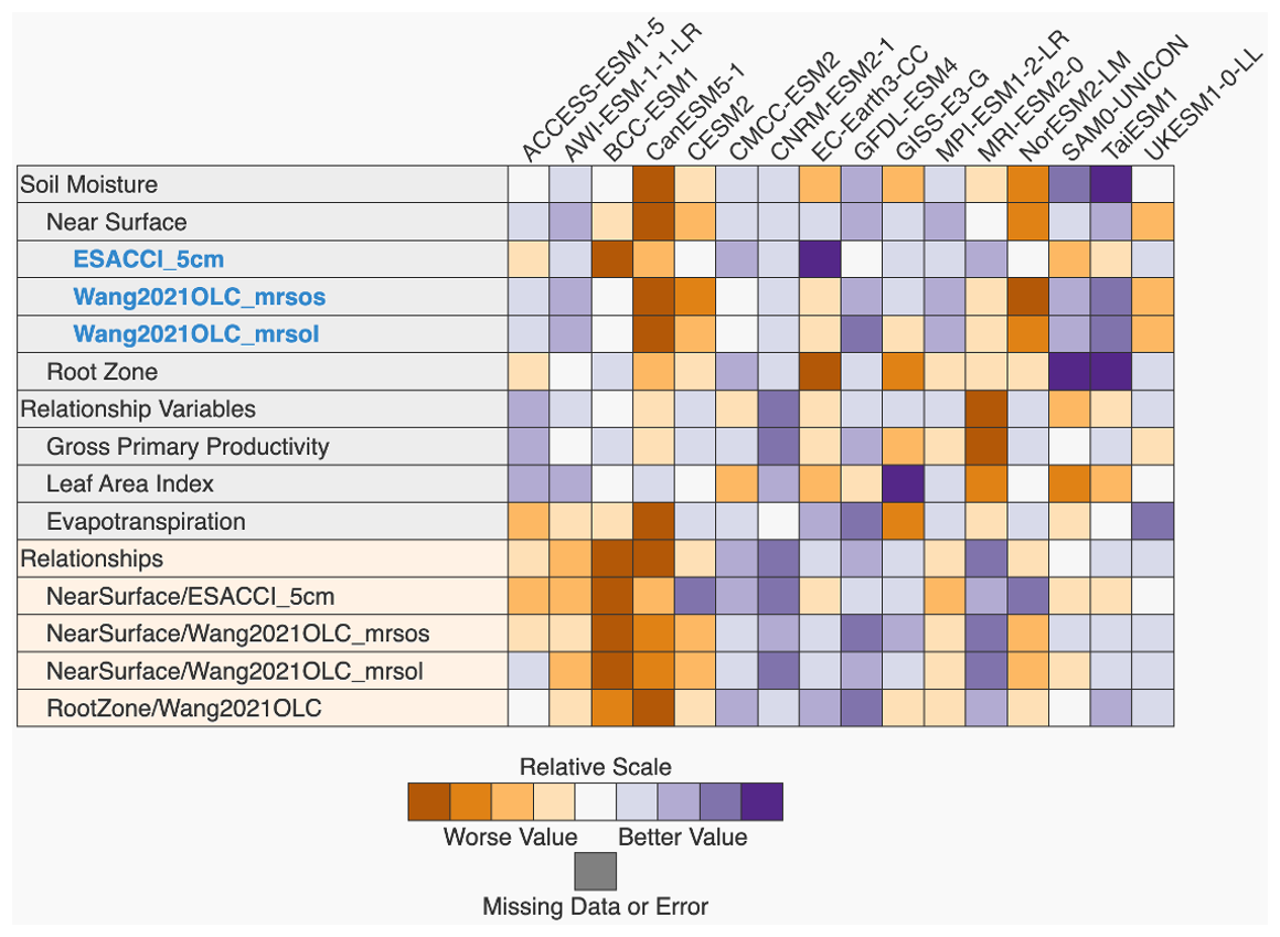
Figure 3 Benchmarking results from the ILAMB global run. Each model is compared against observational datasets: ESA-CCI Surface SM [m³ m⁻³] (top 5 cm), Wang2021OLC Surface SM [m³ m⁻³] (top 10 cm), Wang2021OLC Rootzone SM [m³ m⁻³] (top 100 cm), WECANN GPP [g m⁻² d⁻¹ ], AVH15C1 LAI [unitless], and GLEAMv3.3a ET [mm d⁻¹ ]. Additionally, the relationships between soil moisture and ecohydrological variables (GPP, LAI, and ET) are also benchmarked. Purple represents better relative skill, while orange indicates relatively worse performance.

3.2 Surface and Rootzone Soil Moisture

The evaluation of surface and rootzone SM highlights sensitivity both to the observational reference and to the soil depth considered. When surface SM is evaluated using ESA-CCI (top 5 cm) and Wang2021OLC (top 10 cm), roughly half of the models change their relative skill ranking while others remain similar (Fig. 3), indicating that benchmarking outcomes at shallow depths depend in part on the choice of observational dataset. In contrast, when different model representations of shallow SM (mrsos and mrsol integrated to 10 cm) are evaluated against Wang2021OLC, most models retain similar rankings, suggesting relatively consistent performance across comparable near-surface depths within a common benchmark. Rootzone SM (0–100 cm), also evaluated against Wang2021OLC, shows a mixture of stable and shifting rankings relative to the surface evaluation: several models change skill category or show modest shifts, while many remain broadly similar. Together, these patterns indicate that differences among observational products influence surface benchmarking outcomes, while depth-dependent differences in model performance emerge more clearly when extending the evaluation to the rootzone.

As noted in Sect. 2.2, differences in model vertical discretization introduce an additional source of uncertainty, particularly for surface SM. Some models have first soil layers that are deeper than 5 cm, so integrating mrsol to 5 cm to match ESA-CCI can introduce representational errors, which likely contributes to part of the spread in surface SM performance. This structural mismatch between model layers and observational depth definitions complicates direct comparisons and underscores the challenges of benchmarking near-surface SM consistently across models.

The Taylor diagram analysis (Fig. 4), based on monthly mean fields from both models and observational datasets, further illustrates systematic differences between surface and rootzone performance. Across models, correlations with observed surface SM are generally higher than agreement in variability, indicating that models tend to better capture relative wetness and dryness patterns than absolute soil moisture magnitudes. In contrast, rootzone SM exhibits a systematic overestimation of variability across nearly all models. This suggests that ESMs tend to simulate larger fluctuations in deeper soil moisture than indicated by available reference data, pointing to a persistent challenge in representing subsurface water storage and buffering processes. At the same time, the limited availability and greater uncertainty of deep soil moisture observations likely contribute to the reduced observed variability at depth, implying that part of the model–data discrepancy may reflect observational limitations as well as model deficiencies. Together, these results indicate that while many models achieve reasonable performance for surface SM patterns, substantial challenges remain in representing the magnitude and variability of rootzone SM. The contrast between relatively robust surface correlations and systematically inflated deep-soil variability highlights the importance of improving subsurface hydrological processes and their vertical coupling in land surface models.

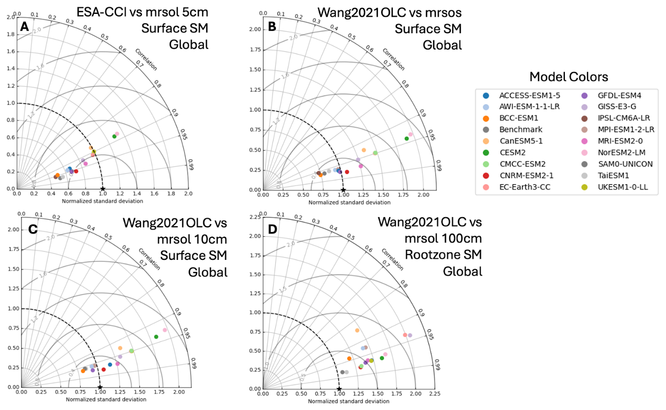
Figure 4 Taylor diagrams evaluating the performance of CMIP6 model SM simulations compared to different observational datasets: (A) Surface SM from ESA-CCI (top 5 cm), (B) Wang2021OLC Surface SM using mrsos from the models (top 10 cm), (C) Wang2021OLC Surface SM using mrsol from the models (top 10 cm), and (D) Wang2021OLC Rootzone SM (top 100 cm).

3.3 Ecohydrological Variables

The evaluation of ecohydrological variables (GPP, LAI, and ET) reveals substantial diversity in model performance across variables and across models (Fig. 3). Unlike soil moisture, where some coherence in relative ranking is evident, models that perform well for one ecohydrological variable often perform poorly for others, resulting in a wide spread of rankings and few consistently high-performing models across all three benchmarks. This lack of coherence highlights the difficulty of achieving balanced realism in vegetation productivity, canopy structure, and surface fluxes within a single model framework.

The Taylor diagram analysis (Fig. 5), based on monthly mean fields from models and observational datasets, further illustrates systematic differences in how these variables are represented. Across most models, both GPP and LAI exhibit a pronounced high bias in variability, indicating that models tend to overestimate fluctuations in vegetation productivity and canopy structure relative to observations. In contrast, ET generally shows stronger agreement with observations, both in terms of spatial correlation and variability. This pattern suggests that while models capture the large-scale controls on surface energy and water fluxes relatively well, they tend to exaggerate the amplitude of vegetation responses.

The comparatively stronger performance in ET likely reflects, at least in part, tighter physical constraints through the surface energy balance and the availability of multiple independent observational products used to evaluate and calibrate this variable. Although transpiration is fundamentally a vegetation-controlled process and is represented in land models through the same canopy and stomatal conductance formulations that regulate carbon uptake, ET can nonetheless appear better constrained because it is subject to additional physical and observational constraints.

In addition, this relatively strong ET skill may also arise from compensating parameter choices that mask deficiencies in soil moisture representation. For example, biases in soil hydraulic properties or effective soil water holding capacity may compensate for missing or simplified processes such as groundwater interactions or root water uptake, allowing models to reproduce realistic surface fluxes despite underlying errors in subsurface moisture dynamics. By comparison, GPP and LAI are influenced by a broader set of interacting biological and phenological processes, which are represented differently across models and remain more weakly constrained by observations (Massoud et al., 2019; Li et al., 2025b). As a result, larger inter-model spread and systematic variability biases in GPP and LAI are not unexpected, even in cases where ET appears relatively well simulated.

Together, these results indicate that skill in simulating surface fluxes does not necessarily imply comparable skill in representing vegetation structure or productivity, and that improvements in ecohydrological realism will likely require more consistent treatment of vegetation dynamics in addition to improvements in hydrological processes.

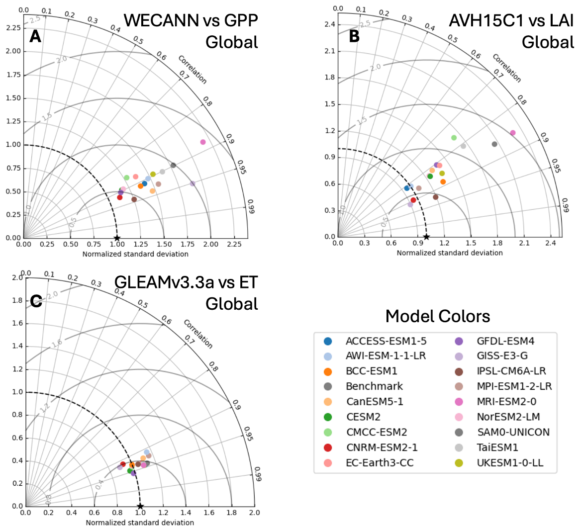
Figure 5 Taylor diagrams evaluating the performance of CMIP6 models in simulating ecohydrologic variables: (A) Gross Primary Productivity (GPP) from WECANN, (B) Leaf Area Index (LAI) from AVH15C1, and (C) Evapotranspiration (ET) from GLEAMv3.3a.

3.4 Relationship of Soil Moisture to Ecohydrological Variables

The relationship between soil moisture and ecohydrological variables provides a more stringent test of model behavior than evaluation of the individual variables alone. Figures 6 and 7 illustrate these relationships for the ACCESS-ESM1-5 model using two different observational surface SM products, based on monthly mean fields consistent with the temporal resolution of the analysis. The comparisons reveal that apparent agreement in individual variables does not necessarily translate into agreement in their coupled behavior, with notable differences emerging depending on the benchmark dataset and the depth of soil moisture considered.

When evaluated against the ESA-CCI surface SM product (0–5 cm; Fig. 6), models exhibit substantial discrepancies in the diagnosed relationships between SM and GPP, LAI, and ET, indicating that vegetation sensitivity to near-surface moisture is not consistently represented. In contrast, when the Wang2021OLC product is used with SM integrated to 10 cm (Fig. 7), agreement between models and observations improves for most variables, suggesting that part of the mismatch in surface-based comparisons arises from differences in observational products and soil depth representation. This highlights the strong sensitivity of coupling diagnostics to both the choice of reference dataset and the effective depth over which soil moisture is evaluated. We note that the climatological fields shown in Figs. 6 and 7 are computed within ILAMB from the available gridded data over the evaluation period. Because the ESA-CCI product contains spatial and temporal gaps in coverage, the resulting inferred climatological means and relationships may be influenced by incomplete sampling, potentially affecting the model–data comparison.

Extending this analysis across the full CMIP6 ensemble (Fig. 8) confirms that coupling skill varies widely among models and does not simply mirror performance in the individual SM or ecohydrological variables. Some models that perform well for SM or for GPP, LAI, and ET individually nevertheless show weak performance in the coupling metrics, indicating that reproducing realistic mean states or variability is insufficient to guarantee realistic dynamic sensitivity between soil moisture and ecosystem processes. Conversely, other models exhibit relatively stronger coupling skill despite more modest performance in the individual variables, underscoring that different aspects of model behavior are being tested by these diagnostics.

Together, these results demonstrate that benchmarking SM–ecosystem relationships provides complementary information to traditional state-based evaluations. The systematic differences in coupling performance across models and datasets point to persistent challenges in representing how soil moisture anomalies propagate into vegetation and surface flux responses, and motivate further examination of the underlying structural differences among land models.

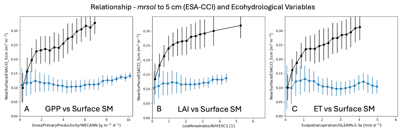
Figure 6 Relationship of SM (y-axis) versus ecohydrological variables (x-axis) shown through dot-and-whisker plots for the ACCESS-ESM1-5 model (blue) and observations (black). The ESA-CCI SM product (typically to 5 cm) is used here for SM, compared to the ACCESS-ESM1-5 model's SM integrated to the same depth (mrsol to 5 cm). The relationship of these SM estimates are shown for (a) WECANN GPP, (b) AVH15C1 LAI, and (c) GLEAMv3.3a ET at the global scale. Whiskers indicate interquartile ranges across land grid cells. These plots reveal a significant discrepancy between the model and observations when using ESA-CCI as the SM benchmark.

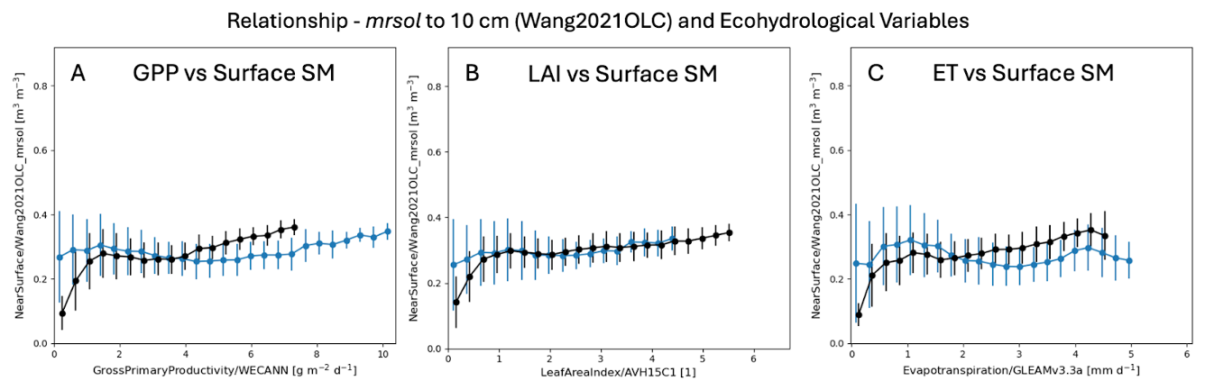
Figure 7 Similar to Fig. 6, but using the Wang2021OLC SM product (integrated to 10 cm) and the corresponding ACCESS-ESM1-5 model SM at the same depth (mrsol to 10 cm). Dot-and-whisker plots show the relationship of soil moisture (y-axis) versus (a) WECANN GPP, (b) AVH15C1 LAI, and (c) GLEAMv3.3a ET for both model (blue) and observations (black) at the global scale. Whiskers represent interquartile ranges. Compared to Fig. 6, these plots demonstrate a marked reduction in discrepancies between modeled and observed relationships.

3.5 Other ILAMB capabilities: Köppen Classification

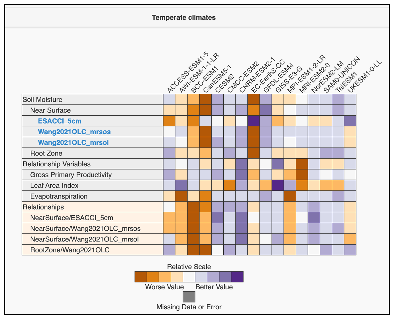
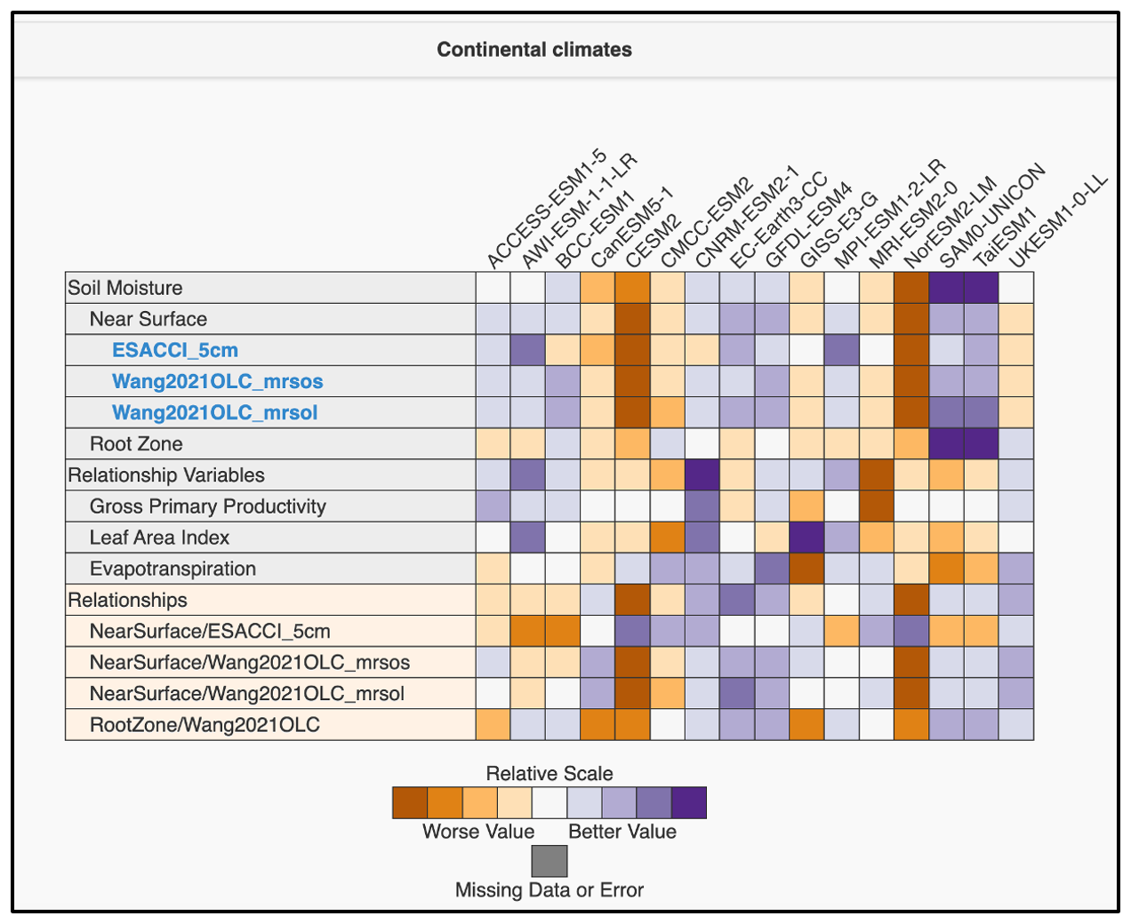
While the preceding analyses focus on global-scale benchmarking, one of ILAMB's key strengths is its ability to evaluate model performance within specific biogeographic regimes. Using Köppen classifications, we assess model behavior across Tropical, Desert and Semi-arid, Temperate, and Continental climate zones (Fig. A4). The regional results from ILAMB (Figs. A5–A9) reveal that model performance is strongly dependent on the climate zone and that global scores can obscure substantial regional contrasts.

In the Tropical region (Figs. A5–A6), CLM5-based models (CESM2 and NorESM2-LM) exhibit consistently high skill across soil moisture, ecohydrological variables, and their relationships, indicating coherent performance in energy- and water-rich environments. In contrast, JSBACH-based models (MPI-ESM1-2-LR and AWI-ESM-1-1-LR) show systematically weaker performance across many of these diagnostics, while UKESM1-0-LL (JULES) exhibits mixed behavior, with relatively stronger performance for rootzone SM and surface fluxes but weaker performance for surface SM and GPP. These patterns suggest that model differences that are muted in global averages can become more pronounced when evaluated in climate regimes dominated by deep rooting, strong transpiration control, and tight soil–vegetation coupling.

In Desert and Semi-arid regions (Fig. A7), CLM5-based models again show generally strong performance across most variables, although skill in rootzone SM is reduced, leading to weaker coupling metrics involving deep soil moisture. JSBACH-based models tend to perform relatively well for soil moisture states but less well for ecohydrological variables, resulting in degraded coupling diagnostics. UKESM1-0-LL again shows mixed behavior, with relatively strong performance for rootzone SM and ET but weaker performance for surface SM and GPP, and correspondingly weaker coupling metrics. These results highlight that in water-limited environments, differences in how soil moisture anomalies propagate into vegetation and flux responses become particularly important.

In Temperate regions (Fig. A8), CLM5-based models maintain generally high performance across most benchmarks, although some degradation is evident for LAI. JSBACH-based models show relatively good performance for surface SM and LAI but weaker performance for rootzone SM, GPP, and ET, leading to poor coupling metrics. UKESM1-0-LL again exhibits stronger performance for rootzone SM and ecohydrological variables than for surface SM, with coupling metrics remaining comparatively weak. This intermediate regime underscores the growing importance of vertical soil moisture structure and rooting depth in shaping both state and coupling performance.

The Continental (high-latitude) region (Fig. A9) shows the most pronounced divergence among models. Here, CLM5-based models exhibit markedly degraded performance across soil moisture, ecohydrological variables, and their relationships, likely reflecting the strong influence of cold-region processes such as organic soils, freeze–thaw dynamics, and high soil porosity, which lead to substantially higher simulated soil moisture than indicated by current observational products. In contrast, JSBACH-based models show relatively good performance for surface SM and ecohydrological variables but weaker performance for rootzone SM, resulting in depth-dependent differences in coupling skill. These results demonstrate that high-latitude regions pose distinct challenges for both observations and models, and that process representations that improve performance in one climate regime may degrade it in another.

Taken together, the regional diagnostics show that no single model performs uniformly well across all climate regimes and benchmarks. The strong regime dependence of model skill highlights the importance of regional evaluation for identifying both strengths and weaknesses that are not evident from global metrics alone, and reinforces the need for process-based interpretation of benchmarking results.

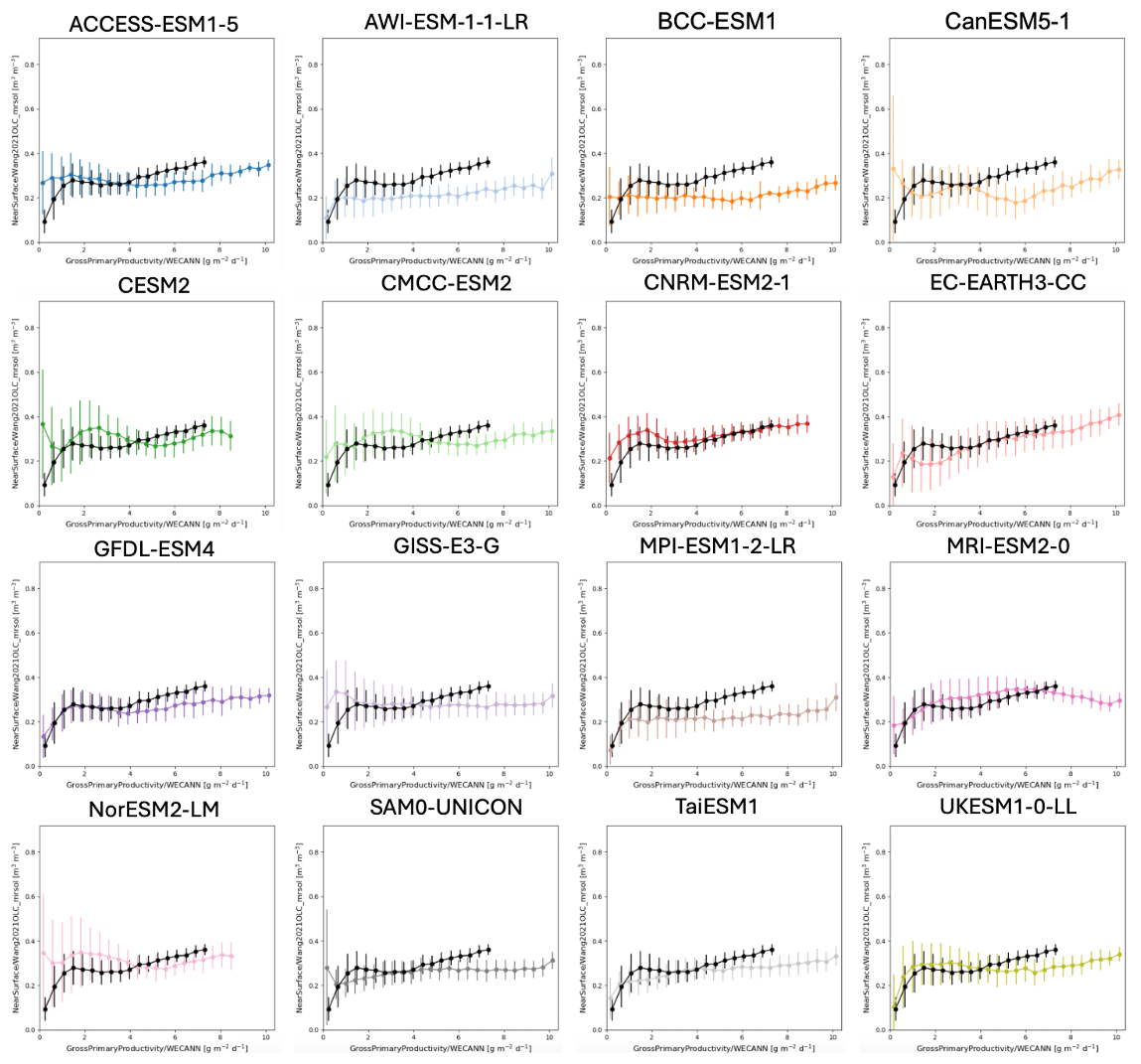
Figure 8 Similar to the bias plots shown in Fig. 7A, but for all models. These plots highlight the observed relationships (black curves) between the surface SM (from the Wang2021OLC top 10 cm SM product) and GPP (from WECANN), as well as the relationship shown in each model (colored curves) using the simulated mrsol to 10 cm and gpp variables.

4 Discussion

4.1 Potential Drivers for Divergences in Model Simulations

The substantial spread in SM estimates among CMIP6 models reflects differences in how land surface models (LSMs) represent key processes and input data, as evidenced by both the global and Köppen-region ILAMB diagnostics (Sect. 3.1 and 3.5). Although precipitation is a major driver of SM, it does not explain much of the mean inter-model variability in this study. Most CMIP6 models simulate similar global mean precipitation rates of approximately 2.5 mm d⁻¹ (Tapiador et al., 2018), suggesting that differences in total precipitation alone are insufficient to account for the spread in simulated SM (see Fig. A1, column “Model Period Mean”). However, the timing and intensity of precipitation events, rather than total amounts, may contribute significantly to model divergence, especially in regions with highly seasonal precipitation regimes where the timing of precipitation governs the length of dry-down periods. This effect is particularly pronounced in seasonally snowmelt-dominated systems (Harpold and Molotch, 2015), where variations in precipitation and snowmelt seasonality strongly influence the partitioning between infiltration, runoff, and ET. Differences in how models represent storm frequency, sub-daily rainfall variability, and snowmelt dynamics can therefore propagate into systematic differences in SM variability and ecohydrological coupling, as seen in the regional results. Similarly, the treatment of soil ice is unlikely to contribute significantly to SM variability in a direct sense, as the CMIP6 definition of SM includes both liquid water and ice, which should be handled consistently across models and is only relevant in cold regions. This implies that other factors, such as soil properties, hydrologic parameterizations, and land–atmosphere feedbacks, are likely more important contributors to the inter-model spread highlighted in Sect. 3.2–3.5.

One important driver is the treatment of soil properties, particularly in high-latitude regions. Models that include representations of organic soils, such as CESM2 and NorESM2-LM, tend to simulate higher SM levels, likely due to the greater water-holding capacity of organic matter. Both models use the CLM5 land surface scheme, which explicitly accounts for organic soil processes in northern latitudes (Lu et al., 2020). This feature provides a plausible explanation for the large positive SM biases seen for these models in the Continental region (Figs. A9 and A3), while also being consistent with their comparatively strong performance in Tropical and Temperate regions (Figs. A5 and A8), where organic-rich soils and strong vegetation–soil coupling are widespread. It remains unclear whether all CMIP6 models have updated their treatment of organic soils to a similar degree, which could contribute to persistent inter-model differences in both SM states and SM–vegetation relationships.

Soil porosity is another critical input affecting SM simulations. Previous work (Dai et al., 2019) has shown that many CMIP5 models used outdated soil maps (e.g., FAO, 2003), and some CMIP6 models may still rely on these legacy datasets. More modern global soil datasets, such as the Harmonized World Soil Database v2.0 (Nachtergaele et al., 2023), the Global Soil Dataset for Earth System Modeling (Shangguan et al., 2014), and SoilGrids (Hengl et al., 2014), offer improved estimates of soil properties, including porosity. Differences in the underlying soil maps and parameter choices may therefore help explain why some models perform well for surface SM but poorly for rootzone SM, or vice versa, as seen in several Köppen regions (Sect. 3.5).

Model-specific representations of hydrologic processes further influence SM estimates and coupling behavior. For example, EC-Earth3-CC consistently simulates high SM values, potentially due to its inclusion of groundwater–soil interactions not present in many other models. With a few exceptions (Oleson et al., 2013; Lawrence et al., 2019), ESMs generally rely on “bucket-type” soil moisture representations that drain water between layers based on thresholds (e.g., field capacity) and rates (e.g., hydraulic conductivity), rather than fully pressure-driven flow as in Richards' equation. Across the CMIP6 ensemble, differences in the number and spacing of soil layers, rooting profiles, ET parameterizations, infiltration schemes, soil hydraulic properties, total soil depth, and lower boundary conditions (e.g., free drainage versus groundwater influence; see Table A1) likely contribute to the contrasting behaviors observed among model families, such as the different surface-versus-rootzone and state-versus-coupling skill patterns seen for CLM5-, JSBACH-, and JULES-based models.

Finally, land–atmosphere feedbacks may also contribute to the inter-model spread. CMIP models have been shown to overestimate the strength of feedbacks between SM and atmospheric variables, including temperature, ET, and surface fluxes (Levine et al., 2016). These exaggerated feedbacks may amplify SM variability and introduce additional divergence across models. For instance, models that strongly couple soil moisture to surface heat fluxes may simulate more aggressive drying or wetting cycles, depending on local conditions (Schumacher et al., 2022), potentially contributing to the widespread pattern of relatively good ET skill but weaker SM–ET coupling seen in several models (Sect. 3.4). The degree of inter-model variability in feedback strength is probably quite high, but further studies are needed to quantify how this affects inter-model spread in SM (Vogel et al., 2018; Talib et al., 2023).

In summary, the observed variability in SM simulations across CMIP6 models likely stems from a combination of factors, including differences in soil properties, legacy input datasets, precipitation event timing, hydrologic parameterizations, vertical structure and boundary conditions, and land–atmosphere feedbacks. The regime-dependent patterns revealed by the Köppen analysis suggest that these factors operate differently across climate zones, reinforcing the need for both global and regional diagnostics when evaluating and improving SM representation in ESMs.

4.2 Shared characteristics of models with similar performance

The global and regional ILAMB diagnostics reveal clear clustering of model behavior by land surface framework (Sect. 3.1 and 3.5; Table A1), indicating that structural choices in land model formulation exert a first-order control on both state and coupling performance. Models that share a common land surface model tend to exhibit similar strengths and weaknesses across soil moisture (SM), ecohydrological variables, and their interrelationships, suggesting that performance differences are not purely idiosyncratic but are linked to shared process representations.

CESM2 and NorESM2-LM, which both use CLM5, provide a clear example of this structural coherence. These models show relatively strong and internally consistent performance for ecohydrological variables (GPP, LAI, and ET) and their coupling to SM across several regions, particularly in the Tropical and Temperate zones (Sect. 3.5, Figs. A5 and A8). This behavior is consistent with CLM5's more detailed treatment of soil hydrology and explicit soil–plant hydraulic stress, which promotes coherent interactions between soil water availability, transpiration, and photosynthesis (Table A1). At the same time, both models exhibit degraded performance in the Continental (high-latitude) region, where their inclusion of organic soils and cold-region processes leads to systematically higher simulated SM than indicated by current observational products (Fig. A9). This combination of strong ecohydrological coupling but biased SM states highlights how a given structural choice can improve process coherence while simultaneously introducing regional biases.

In contrast, the JSBACH-based models (MPI-ESM1-2-LR and AWI-ESM-1-1-LR) tend to show relatively good performance for some SM state variables, particularly near the surface in several regions, but weaker performance for ecohydrological variables and, notably, for SM–vegetation coupling metrics. This pattern is especially evident in arid and temperate regimes (Sect. 3.5), where these models often reproduce mean SM reasonably well but fail to translate SM variability into realistic vegetation or flux responses. A plausible explanation is that JSBACH relies on more implicit vegetation water-stress formulations and simplified soil–plant coupling (Table A1), which may limit the model's ability to propagate soil moisture anomalies consistently into photosynthesis and transpiration, even when the soil moisture state itself is reasonably represented.

UKESM1-0-LL (JULES) exhibits a different, mixed behavior. This model often shows weaker performance for surface SM but comparatively better performance for rootzone SM and surface fluxes, along with moderate skill in some coupling metrics. This depth-dependent pattern is consistent with JULES's prescribed root distributions and implicit soil moisture stress functions, which can yield reasonable integrated flux responses while still allowing biases in shallow soil layers (Table A1). The recurring finding that UKESM1-0-LL captures some aspects of ecohydrological behavior despite weaker SM states reinforces the idea that realistic fluxes do not necessarily guarantee realistic subsurface moisture dynamics.

Taken together, these results demonstrate that similarities in land surface model architecture translate into recognizable performance “signatures” across both global and regional benchmarks. They also show that models can achieve good performance in individual variables while still failing to capture the correct coupling between soil moisture and ecosystem processes. This underscores the importance of evaluating not only state variables but also cross-variable coherence, and suggests that targeted improvements to soil hydrology, rooting depth distributions, and soil–plant coupling schemes could yield broad benefits across multiple aspects of model performance.

4.3 Consideration of uncertainty and limitations in the benchmark results

Evaluating model performance inherently involves uncertainty, both from observational datasets and from model representations. To better characterize this uncertainty, we employed multiple observational products for surface and rootzone SM, including ESA-CCI and Wang2021OLC surface SM, as well as Wang2021OLC rootzone SM. By comparing models against more than one observational reference, we aimed to capture a broader envelope of observational variability, rather than relying on any single product that may contain its own structural or systematic biases. We reiterate that none of the benchmark datasets used here represents a definitive truth, and that our multi-product approach is intended to reduce dependence on any single reference and to better characterize observational uncertainty. Similarly, we assessed different model representations of SM, including the mrsos and mrsol variables integrated to 5, 10, and 100 cm depths, to examine how model configuration affects evaluation outcomes.

We note that GPP and LAI are integrative ecosystem variables influenced by multiple interacting processes beyond soil moisture alone, and therefore discrepancies in SM–GPP or SM–LAI relationships cannot be interpreted mechanistically as arising solely from deficiencies in soil hydrology. In this study, these relationships are instead used to assess whether models reproduce the emergent ecosystem-scale coupling between soil moisture variability and vegetation functioning. More process-level hydrological quantities, such as runoff, drainage, or evaporation–transpiration partitioning, would be valuable for mechanistic diagnosis of soil moisture controls, but their use as global benchmarking targets is currently limited by observational availability and consistency. We therefore focus on GPP, LAI, and ET as comparatively well-constrained, widely evaluated ecosystem-scale diagnostics, while acknowledging the associated limitations in process-level attribution.

Soil moisture presents unique challenges in benchmarking due to the diversity and limitations of observational data sources. Satellite-derived products offer broad spatial coverage but are limited to shallow depths and may have coarser resolution for passive microwave technology, whereas active microwave retrievals can achieve higher resolution but are subject to greater uncertainty from surface roughness and vegetation structure (Zeng et al., 2023). In contrast, in-situ observations provide deeper and more accurate point measurements but are geographically sparse and face substantial scaling challenges when compared against ESM grid cells. While our study did not include in-situ datasets, their inclusion could strengthen future benchmarks, particularly for deeper soil layers and for regions where satellite coverage is limited. The variation in spatial resolution, vertical depth coverage, and methodological differences between observational datasets contributes to uncertainty in benchmarking, and any conclusions drawn from SM comparisons, especially in data-sparse regions such as high latitudes and arid zones, should be interpreted within this context.

To address these complexities, we adopted a multi-product comparison approach. However, additional strategies may further enhance benchmarking efforts. In atmospheric science, for example, it is common to evaluate models not only against individual datasets but also against an ensemble of observations (Yamaguchi et al., 2016), which helps define a consensus observational baseline. While this strategy is less frequently used in the SM modeling community, it may offer a valuable pathway forward, particularly when observational datasets diverge or when no single product can be considered definitively superior.

Beyond observational uncertainty, ensemble modeling (using a collection of model runs or parameter sets) can also help characterize structural and parametric uncertainty within the models themselves. While not implemented in this study, future benchmarking efforts could benefit from integrating probabilistic or ensemble-based approaches to better understand model sensitivity (cf. Massoud et al., 2019) and confidence in simulated soil moisture.

5 Conclusions

This study evaluated the performance of 16 CMIP6 models in simulating key land surface and ecohydrological variables, including surface and rootzone soil moisture (SM), gross primary productivity (GPP), leaf area index (LAI), and evapotranspiration (ET), using the ILAMB framework. By combining state-variable benchmarks with diagnostics of SM–ecohydrology coupling and regional (Köppen) analyses, we provide a multi-faceted assessment of land model behavior. The main findings are summarized as follows:

• i.

  Model performance in simulating soil moisture (SM) varies substantially depending on the observational benchmark used. For example, some models (e.g., EC-Earth3-CC) perform well against ESA-CCI surface SM but perform substantially worse relative to the Wang2021OLC product. This sensitivity highlights the importance of using multiple observational references to better characterize uncertainty and avoid conclusions based on a single dataset.

• ii.

  Model skill differs markedly across variables and reflects structural similarities among land surface model frameworks. For instance, CESM2 and NorESM2-LM exhibit relatively strong performance for ecohydrological variables (GPP, LAI, and ET) but show persistent SM biases in high-latitude regions. These shared behaviors reflect their common use of the CLM5 land surface model and illustrate how structural choices shape both strengths and weaknesses in simulated land surface states and fluxes. In particular, models with more explicit soil–plant hydraulic coupling, such as CLM5-based models, tend to reproduce SM–vegetation relationships more consistently across regions, whereas models relying on more implicit vegetation water-stress formulations (e.g., JSBACH- and JULES-based models) more often reproduce soil moisture states without fully capturing the associated vegetation or flux responses.

• iii.

  Evaluating SM–ecohydrology relationships further shows that models more consistently reproduce observed coupling patterns when assessed against the Wang2021OLC dataset than against ESA-CCI. This suggests that deeper soil moisture estimates may provide a more stable reference for diagnosing vegetation–water interactions, while also reinforcing that good performance in individual variables does not necessarily imply realistic cross-variable sensitivity.

• iv.

  Model skill also varies strongly by climate regime. For example, CESM2 and NorESM2-LM perform relatively well in Tropical and Temperate regions but degrade substantially in Continental (high-latitude) zones, where cold-region processes and organic soils play a larger role. These results highlight the limitations of relying on global mean scores alone and demonstrate the value of regional benchmarking for diagnosing where and why models succeed or fail.

Taken together, these results indicate that no single CMIP6 model performs best across all variables, coupling metrics, or regions. Instead, performance patterns often cluster by land surface model family, suggesting that structural choices in soil hydrology, rooting representation, and soil–plant coupling influence both soil moisture states and ecohydrological interactions. The ILAMB framework therefore provides a useful approach not only for benchmarking individual variables but also for diagnosing cross-variable coherence and regional dependencies in model behavior.

Future work should expand these benchmarking efforts by incorporating in-situ observations, applying ensemble-based and probabilistic approaches to both models and observations, and further refining regional analyses. Such developments will be important for improving constraints on soil moisture dynamics, strengthening understanding of land–atmosphere coupling, and guiding the development of next-generation Earth system models, including those participating in CMIP7.

Appendix A

Table A1 Overview of key land surface process representations for some of the selected CMIP6 models used in this study, including hydrology scheme, root distribution, lower boundary condition, and treatment of plant hydraulics. This table provides structural context for interpreting differences in soil moisture, ecohydrological variables, and their coupling across models. Sources for each entry are listed in the table. Because process-level documentation is not consistently available for all CMIP6 models, this table summarizes key characteristics only for models with clearly documented information in the literature.

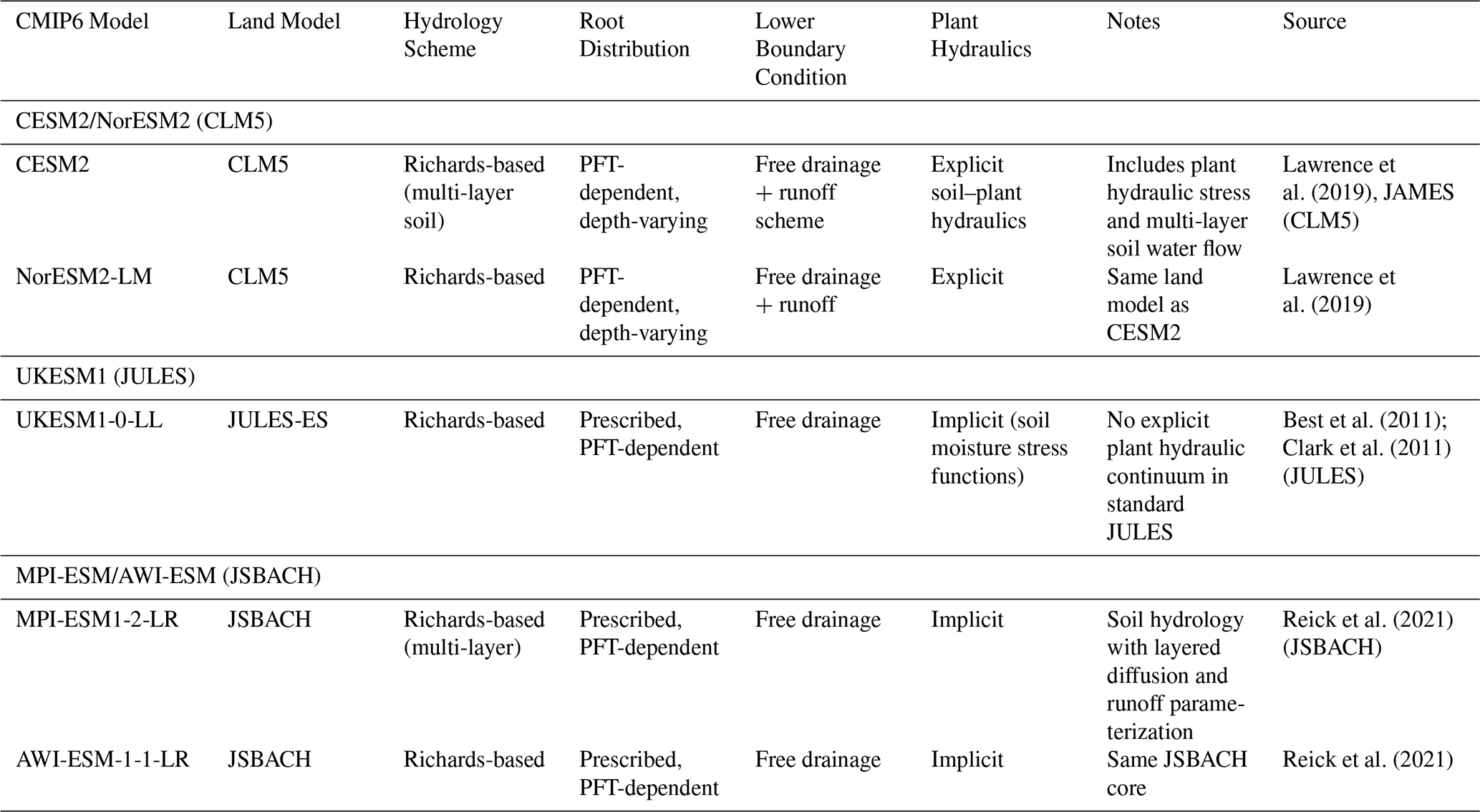
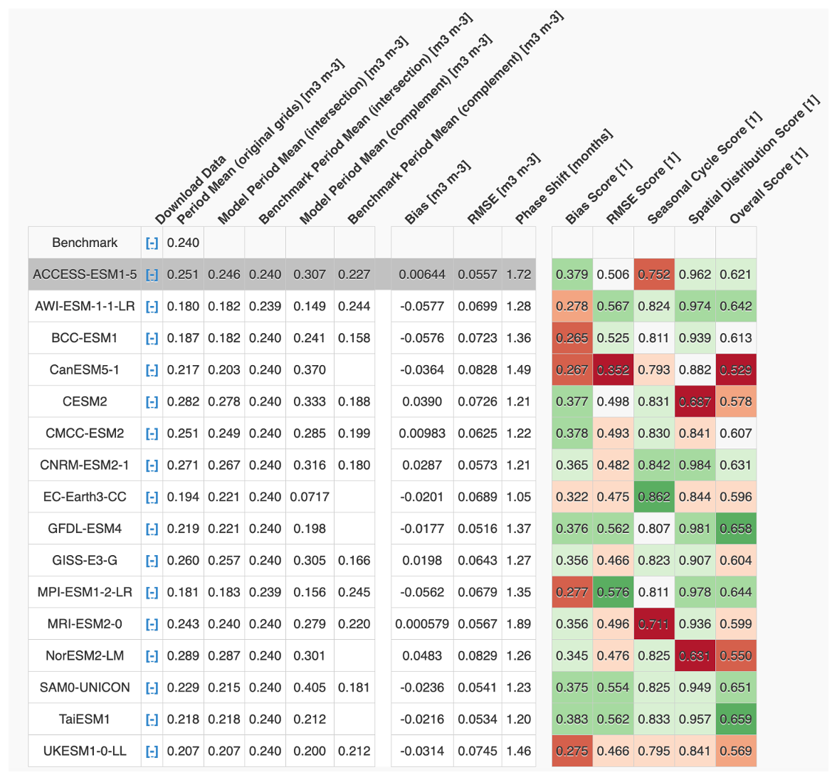
Figure A1 Evaluation of global simulations of SM using the mrsol variable to 10 cm, compared to the Wang et al. (2021) dataset at the same depth. The various metrics shown are the different benchmark scores used in the ILAMB evaluation, including Bias Score, RMSE Score, Seasonal Cycle Score, and Spatial Distribution Score. These scores contribute to the final benchmark, represented here as the Overall Score, and are the results that are presented in Fig. 3 (and Figs. S5 and S7–9).

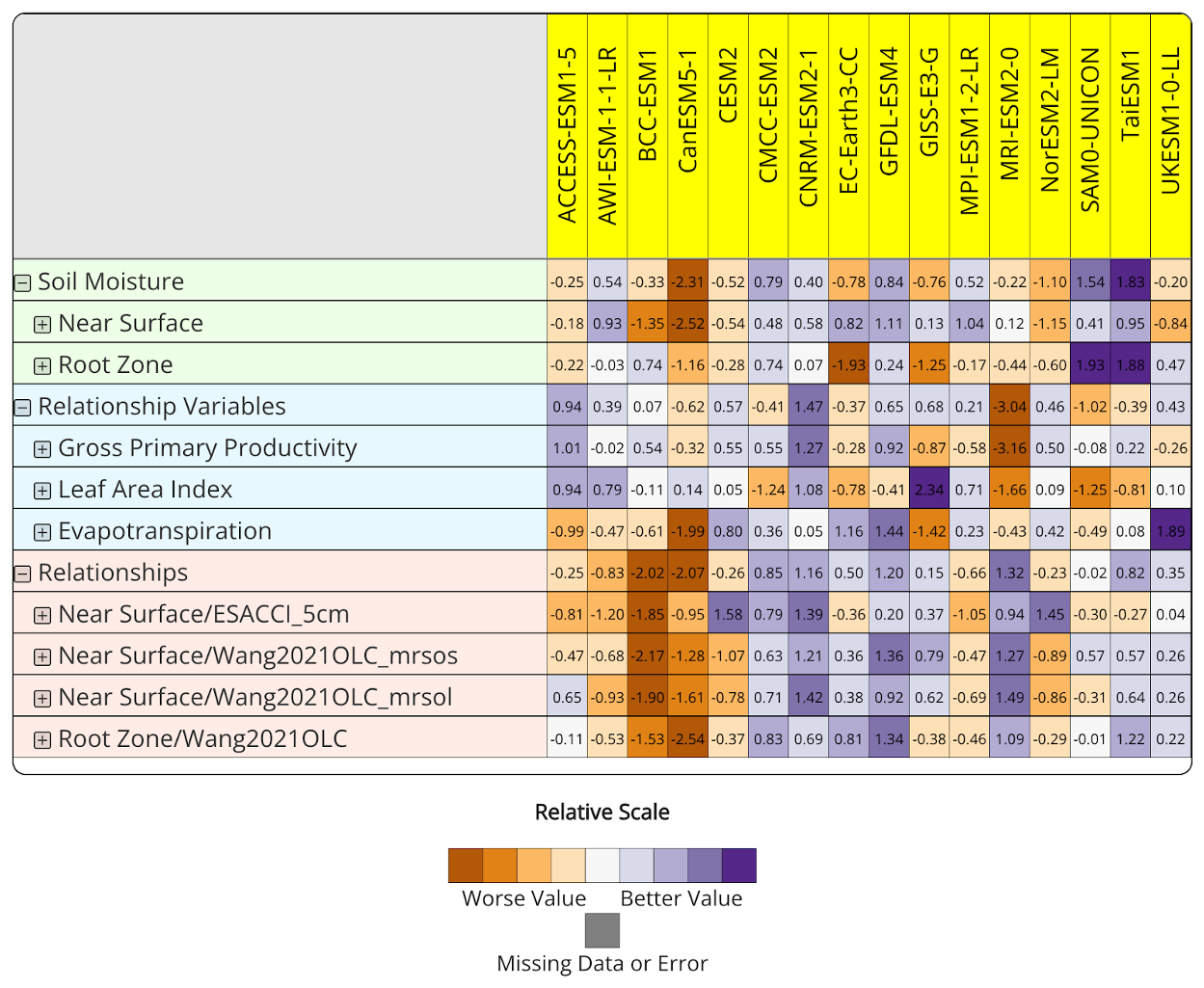
Figure A2 Overall scores that provide the ILAMB results in Fig. 3 are depicted numerically here.

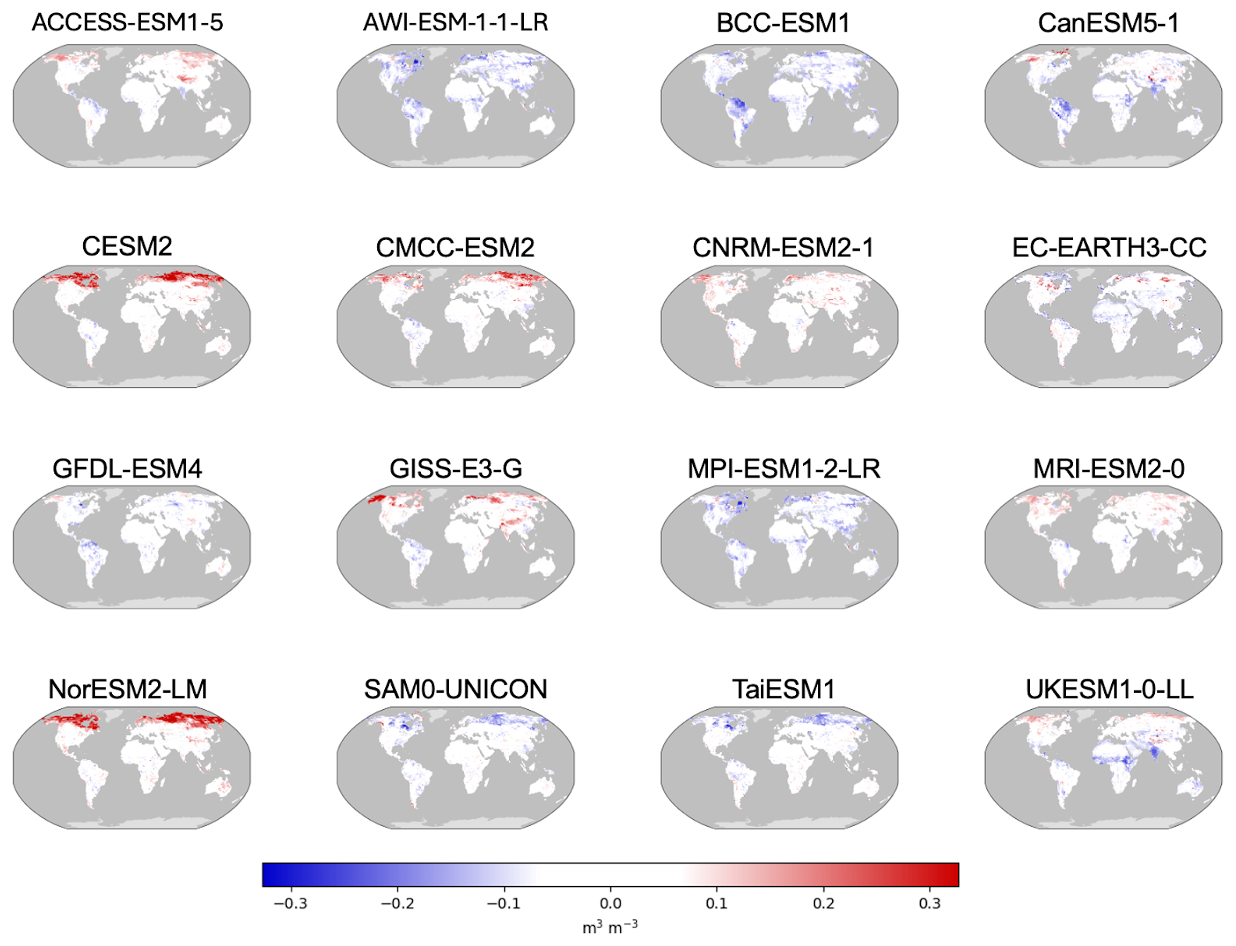
Figure A3 Bias plots (in m³ m⁻³) comparing Wang2021OLC top 10 cm SM product to the mrsol variable up to 10 cm for all models. The bias is calculated as the difference between model simulations and observations in each grid cell, providing insight into simulated SM performance in various regions around the globe. 

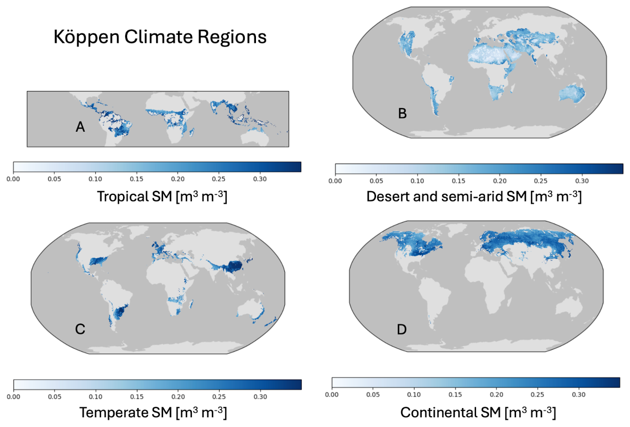
Figure A4 Köppen climate regions evaluated in this study through ILAMB. The default region is “global”, while other regions include (A) Tropical, (B) Desert and Semi-arid, (C) Temperate, and (D) Continental. Regional mean values of surface SM derived from the ESA-CCI product are shown. The ESA-CCI dataset includes some data gaps, particularly in densely forested regions (e.g., the Amazon and Congo), ice-covered areas, and urban zones, due to limitations in microwave satellite observations. These gaps are more prevalent in earlier years and become less frequent over time. However, the primary purpose of this figure is to broadly illustrate the Köppen climate regions rather than serve as a detailed analysis of SM.

Figure A5 ILAMB results similar to Fig. 3, but for the “Tropical” Köppen region.

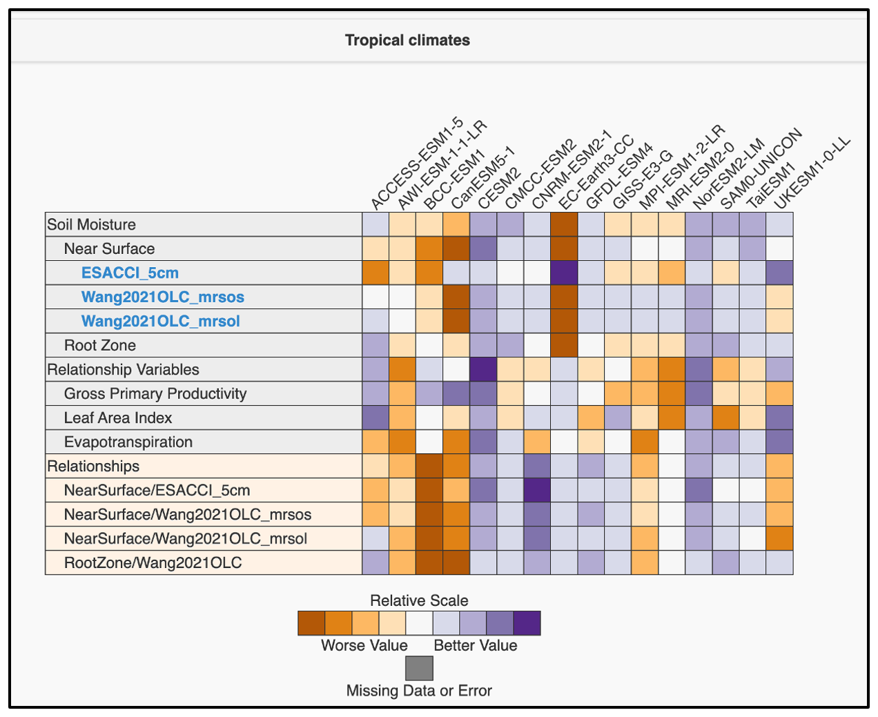
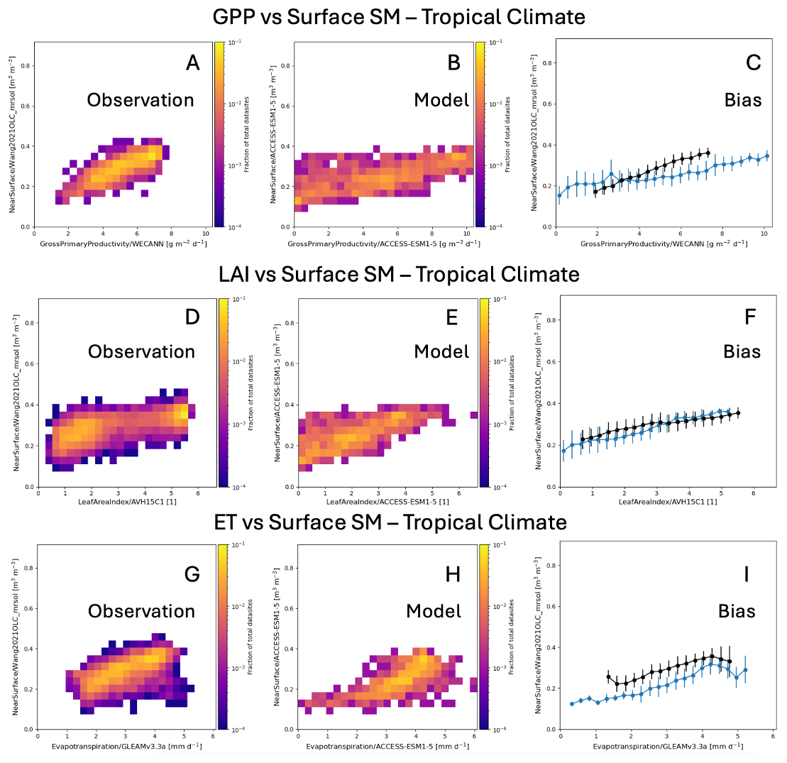
Figure A6 Relationships between surface SM and ecohydrologic variables, similar to Fig. 7, but for the “Tropical” Köppen region. The model results shown here are for the ACCESS-ESM1-5 model. Panels (A), (D), and (G) show the heat maps of the observed relationships, panels (B), (E), and (H) show the heat maps of simulated relationships in the ACCESS-ESM1-5 model, and panels (C), (F), and (I) portray both the observed and simulated relationships in the form of dot and whisker plots for easy comparison.

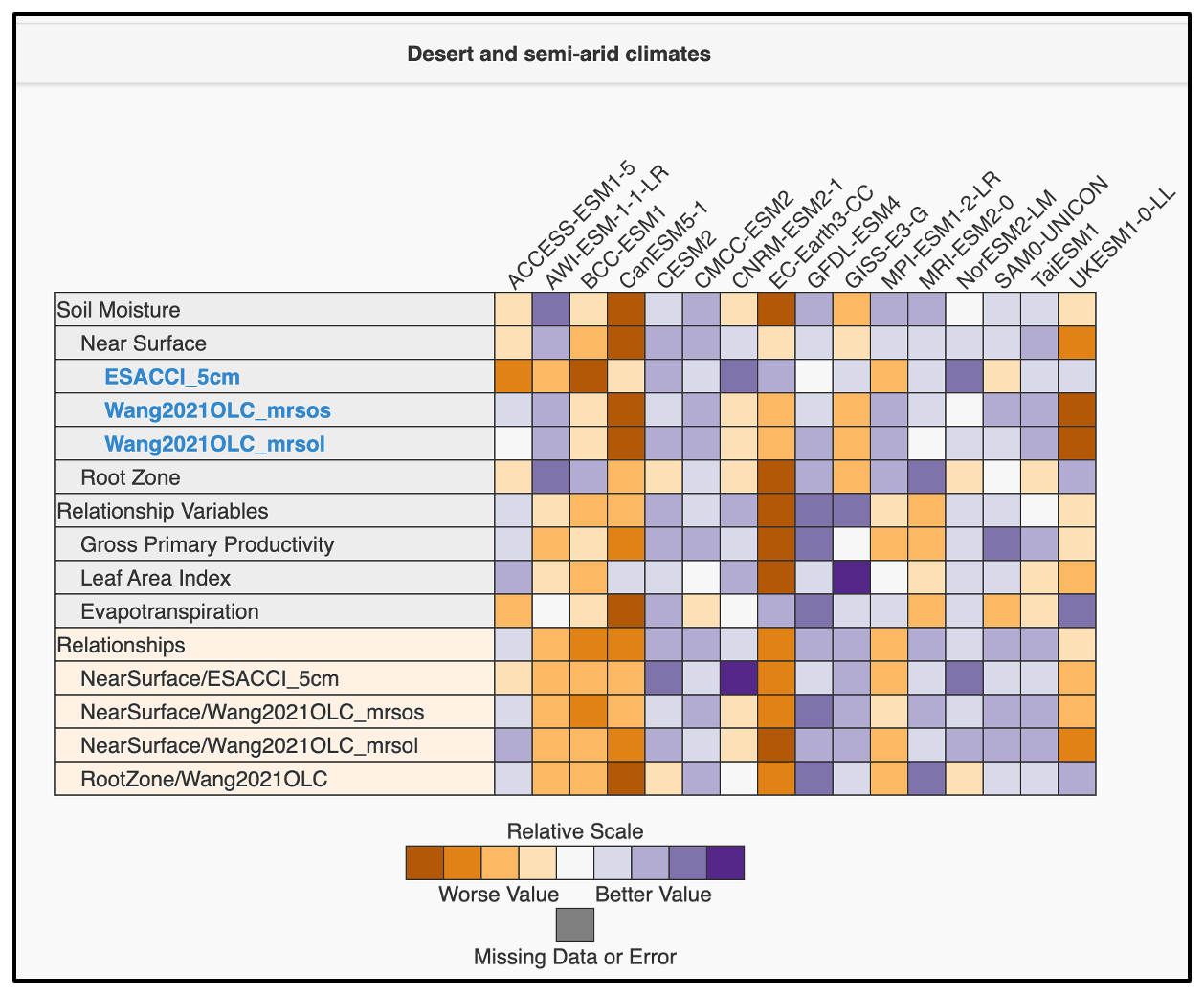
Figure A7 ILAMB results similar to Figs. 3 and A5, but for the “Desert and semi-arid” Köppen region.

Figure A8 ILAMB results similar to Figs. 3 and A5, but for the “Temperate” Köppen region.

Figure A9 ILAMB results similar to Figs. 3 and A5, but for the “Continental” Köppen region.