Controls of the latitudinal migration of the Brazil-Malvinas confluence described in MOM6-SWA14

The distribution and productivity of nutrients, eddy formation, energy dissipation, and other ocean properties are influenced by the variability of Western Boundary Currents (WBCs). In the Southwestern Atlantic, the key features are the Brazil-Malvinas Confluence (BMC) and the North of Brazil Current (NBC). This work investigates them using a 20 year high-resolution ocean model simulation with the Modular Ocean Model version 6 (MOM6) $\mathrm{1}/\mathrm{14}$° configuration. The results reveal a significant deviation in the path and trends of volume transport of the WBCs over the decades. The BMC adjacent region gets saltier and warmer, with increased kinetic energy and transport. Although transport trends in the NBC indicate reduced transport, this results from weaker wind forcing, which reduces the Mixed Layer Depth (MLD) in the simulation and the subsurface transport in the region. The warming in the Brazil Current region triggers a stronger southward flow, resulting in a southward shift of 0.93 ± 0.08° of latitude/decade in the BMC separation. Working against this flow, the propagation of the Kelvin Waves from the Eastern Pacific Ocean induces a northern shift of the BMC, revealed by topographic Kelvin Waves in the spectral analysis. This Pacific-Atlantic inter-basin relation indicated here underscores the importance of propagating Pacific disturbances into the region to maintain the positioning of the BMC and its properties under a warming Atlantic Ocean.

1 Introduction

Recent studies have revealed a relationship between the Southwestern Atlantic Ocean and extreme precipitation events in South America (Rodrigues et al., 2019; Pezzi et al., 2022; Laureanti et al., 2024). The analysis focused on the high-resolution circulation of this ocean was also motivated by oil spills and other accidents polluting the Brazilian coastline, striking important naturally preserved areas (Nobre et al., 2022). Climate studies in the region have focused on heat budgets and trends (Muller et al., 2021; Franco et al., 2020). Improving the description of the ocean circulation features in this region can result in a better understanding of the dynamics, including even that of the CO₂ distribution (Valerio et al., 2021; Bonou et al., 2016). To extend the knowledge of these features, this work focuses on investigating the variability and trends of the Western Boundary Currents (WBCs) in the Southwestern Atlantic Ocean.

The Atlantic Ocean is an energetic region with both surface and undercurrents between the Brazilian eastern coast and the African western coast. Figure 1 illustrates the sea surface currents in this region, including the North Brazil Current (NBC) and the Brazil Current (BC), whose flow is maintained by the southern branch of the South Equatorial Current (sSEC). The sSEC redirects toward South America after originating in the Angola Gyre off the Western African Coast. The BC and the Malvinas Current (MC) confluence at a southward region (Garzoli and Bianchi, 1987; Goni et al., 2011; Combes and Matano, 2014b; Barré et al., 2006; Ferrari et al., 2017; Artana and Provost, 2023), forming the Brazil-Malvinas Confluence (BMC). This region experiences intense oceanic mesoscale activity due to the retroflection of these currents (Oliveira et al., 2009). The MC originates in higher latitudes and flows northward, driven by the Antarctic Circumpolar Current (ACC) (Combes and Matano, 2014b). Meanwhile, the NBC encounters the continental shelf in Northwestern Brazil, where its retroflection generates eddy propagation (Bueno et al., 2022; Garzoli et al., 2004). These are recognized as WBCs, as they path is set along the coastline, comprising unique dynamic properties and interactions with the continental shelf, a common characteristic in the BC, MC, and NBC.

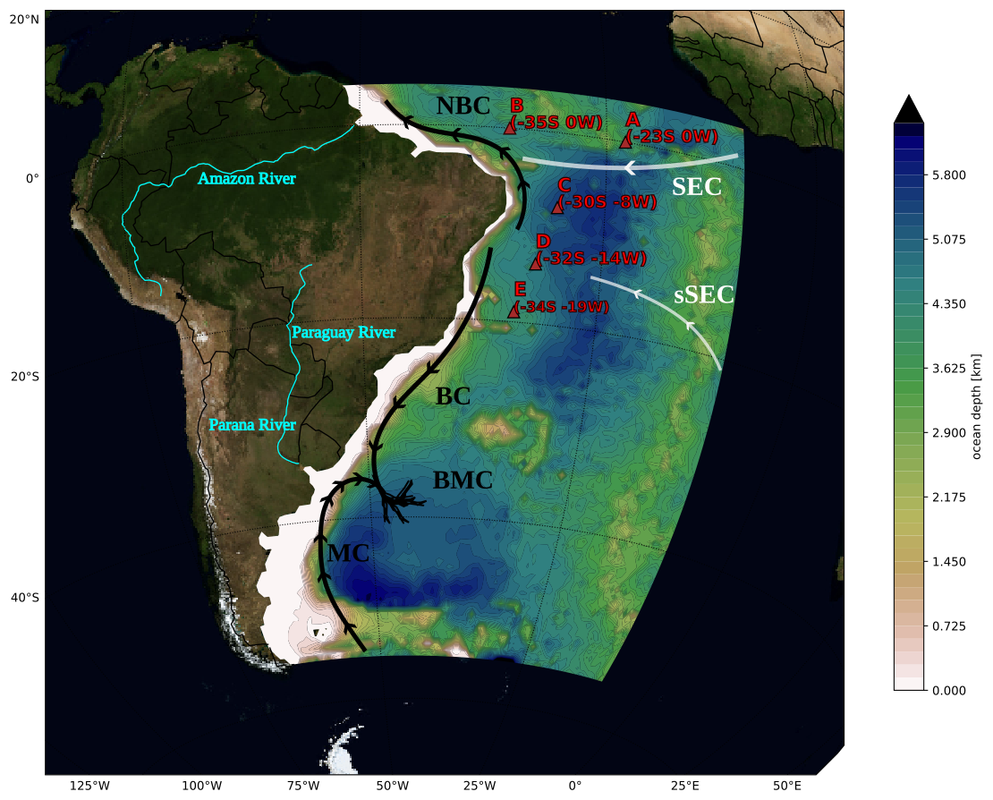
Figure 1 The Southwestern Atlantic simulation domain. The arrows illustrate near-surface currents: from north to south, the South Equatorial Current (SEC) and its southern branch (sSEC), the North Brazil Current (NBC), the Brazil Current (BC), the Malvinas Current (MC) and the Brazil-Malvinas Confluence (BMC). The Western Boundary Currents (WBCs) are in black. The shaded colors indicate the topography in the Southwestern Atlantic Ocean used in MOM6 simulations. The locations of the 5 PIRATA buoys with observational data are in red. The locations of the major rivers in this domain are shown in blue. Satellite images from Blue Marble: Next Generation define the terrain contours by NASA Earth Observatory.

The wind plays a dominant role in the variability of the WBCs (Wunsch and Ferrari, 2004). It impacts the mesoscale structure within the Gulf Stream, which is a WBC in the Northwestern Atlantic Ocean, affecting the Mean Kinetic Energy (MKE) to Eddy Kinetic Energy (EKE) conversions along the coast (Kang et al., 2016). The wind contribution to the BMC variability can be explained by the frequent passage of atmospheric fronts at those latitudes that alter the predominant wind direction and cause sudden reversal of the currents throughout the water column (Campos et al., 2013; Lago et al., 2019). Furthermore, specific analysis of the MC near the Patagonian shelf has demonstrated its modulation by wind stress (Guerrero et al., 2014; Palma et al., 2004; Lago et al., 2019). Additionally, winds also influence the Plata River discharge impacting the BC flow (Piola et al., 2005; Campos et al., 2013). Northwesterly wind-stress anomalies commonly induce heavy runoff over summer, spreading river plumes meridionally. During wintertime, strong southwesterly winds intensify a northward current, causing freshwater discharges from the La Plata Basin to move northward. The seasonality of the atmospheric patterns also contributes to precipitation inputs, which has been considered a contributor to ocean variability (Campos et al., 2013; Lago et al., 2019; Palma et al., 2004). An interannual variability influence near the La Plata Basin is also evident, where the El Niño-Southern Oscillation (ENSO) impacts freshwater discharges (Combes and Matano, 2018). In addition, some studies have recognized the contribution of the South Atlantic Subtropical High (SASH) and the Intertropical Convergence Zone (ITCZ) for the NBC variability. The SASH is the lower-level atmospheric dominant feature of the SEC, impacting the SEC-NBC transport, while the ITCZ predominantly contributes to the Equatorial currents (Lumpkin and Garzoli, 2005; Valerio et al., 2021). Important features related to its variability relate to the propagation of eddies in the NBC retroflection, which results in a deviation of its natural path from 4 to 8° N (Bueno et al., 2022; Valerio et al., 2021).

The highly energetic activity imposes challenges for diagnosing SST in places adjacent to WBC in General Circulation Models (GCMs) (Stock et al., 2015; Adcroft et al., 2019). The oceanic grid resolution is key for simulating the physical processes, as it determines the range of perturbations reproduced by the model (Adcroft et al., 2019; Hallberg, 2013; Chassignet and Xu, 2021). At least a $\mathrm{1}/\mathrm{8}$° resolution is required to explicitly capture the mesoscale baroclinicity in the Southwestern Atlantic, while a resolution higher than $\mathrm{1}/\mathrm{25}$° is recommended for continental shelf regions (Hallberg, 2013). In addition, using a high-resolution ocean bathymetry induces better heat distribution by ocean currents (Griffies et al., 2015). Regional numerical simulations can provide specific diagnostics, including distinct driving mechanisms for shelf circulation. For instance, studies conducted by Palma et al. (2004, 2008) explored the significance of wind and tidal motion in the Patagonian Shelf. The findings indicated that south of 40° S, circulation is primarily influenced by semidiurnal tidal mixing (M2, S2, N2), wind, and the MC. The tidal mixing enhances bottom friction that balances the energy input by the wind stress. Similar outcomes were described in a high-resolution simulation using the Regional Ocean Modelling System (ROMS) (Combes and Matano, 2014a). Local winds contribute significantly to the shelf variability, but adding tides is crucial to replicating the mixing near the coastal region accurately. The MC's transport is highly correlated with the upwelling at the Patagonian shelf break and exhibits an out-of-phase relationship with the BC (Combes and Matano, 2014a).

There are also important WBCs relations driven by the proximity to the coastal slopes (Hughes et al., 2019). The internal variability of the currents and transport in the WBCs offers a broader number of dynamic interactions, different from those in the open ocean. Tropical waves from the Pacific follow the western South American coastline, propagate, and contribute to the coastal dynamics in the Southwest Atlantic Ocean. Poli et al. (2022) reveal that Kelvin wave dispersion and Rossby wave propagation from the Madden-Julian Oscillation are linked to the barotropic and baroclinic components of the coastal trapped waves in the Southwest Atlantic Ocean.

This study aims to extend our understanding of this region by simulating and evaluating the ocean circulation. The relevance of this implementation to global climate studies is the focus on the WBCs, indicating their unique variability and potential drivers. Simulating the Southwestern Atlantic WBCs with a high-resolution framework allows for determining meaningful characteristics of the variability of the mesoscale circulation.

This article is organized as follows: The first two sections detail the model setup and the datasets. The results initially focus on evaluating surface features and vertical structures by comparing them with local observational data in Sect. 3. The analysis discusses the characteristics of the meso- and large-scale circulation within the domain, assessing the contribution of winds and ocean transport to the overall dynamics in the model. Section 4 discusses the seasonal variability and trends of the WBCs. In Sect. 4.3, we focus on the internal and external components of the variability of WBCs. The last section contains the discussion and conclusions, offering an analysis of the variability of the WBCs circulation reproduced by the model.

2 Model and Data

2.1 Model Description and Configuration

The model used in this work is the Modular Ocean Model version 6, developed by the Geophysical Fluid Dynamics Laboratory (GFDL) from the National Oceanic and Atmospheric Administration (NOAA) (Adcroft et al., 2019). The model was designed to represent the ocean's general circulation. The version used in this paper is capable of running on regional configurations as a result of the implementation of open boundary conditions. The horizontal grid extends from longitude 69 to 9° W and from latitude 55° S to 5° N, at $\mathrm{1}/\mathrm{14}$° resolution (approx. 7 km). The model domain uses the topography displayed in Fig. 1. The ocean bathymetry was interpolated from a horizontal resolution of 450 m from the General Bathymetric Chart of the Oceans (GEBCO) (Giribabu et al., 2023). The vertical discretization distributes 75 levels from 3 m up to 6500 m of depth, varying in thickness from 2 m near the surface up to 250 m in the deep ocean. The model uses the z^∗ vertical coordinate, which is a height-based coordinate rescaled with the free surface (Adcroft and Campin, 2004). Under this setup, the model simulation started on 1 January 1997 and ended on 31 December 2016, a total of 20 years. A test run made with the model with a hybrid vertical coordinate is also evaluated from 1997 until 2002, to verify impacts of the vertical discretization.

The model uses initial and boundary conditions data from GLORYS12v1 ocean reanalysis, developed by the Copernicus Marine Environment Monitoring Service (CMEMS), with a daily frequency and an 8 km resolution ($\mathrm{1}/\mathrm{12}$°) (Jean-Michel et al., 2021). The atmospheric forcing is the hourly reanalysis data from the European Centre for Medium-Range Weather Forecasts (ECMWF) fifth generation (ERA5) at 25 km (Hersbach et al., 2023). Ten tidal components from the global model of ocean tides TPXO (Egbert and Erofeeva, 2002) are used in the boundaries and internal domain to force the barotropic conditions through parametrization. The components are four semidiurnal (M2, S2, N2, and K2), four diurnal constituents (K1, O1, P1, Q1), and two long-period constituents (Mm and Mf). The freshwater discharge is from the Global Flood Awareness System (GloFAS) reanalysis dataset (Zsoter et al., 2021). To assimilate natural conditions, chlorophyll estimates from the Sea-viewing Wide Field-of-view Sensor (SeaWiFS-NASA) (NASA, 2018) are inserted in the opacity scheme to modify the estimate of the atmospheric radiation reaching the deepest layers. The MOM6 schemes are based on the physical ocean model configuration of Ross et al. (2023). Parameterizations include the convection Energetic Planetary Boundary Layer (ePBL) approximation (Reichl and Hallberg, 2018), the Fox-Kemper restratification for the mixing layer (Fox-Kemper et al., 2011), while astronomical tides and the Kappa-shear scheme (Jackson et al., 2008) induces interior and bottom mixing, respectively.

2.2 Data for Validation

The 20 year simulation is assessed by comparing mean fields with observational data. The World Ocean Atlas (WOA) temperature and salinity climatology (Locarnini et al., 2019; Zweng et al., 2019) and the Mixed Layer Depth (MLD) climatology from de Boyer Montégut et al. (2004) correspond to the datasets of coarser resolution with a 1° resolution. A local comparison relates the model results to the observational data from 5 buoys from the Pilot Research moored Array in the Tropical Atlantic (PIRATA) project (Servain et al., 1998). The dataset consists of time series and vertical profiles of temperature and salinity over the tropical Atlantic, with five moored buoys in the tropical Atlantic, two on the equator that have data from January 1998 to recent years, and the other three are placed southern, with measurements starting in August 2005. The buoys are A: 0° S 23° W, B: 0° S 35° W, C: 8S° 30° W, D: 14° S 32° W, and E: 19° S 34° W and their locations are shown in Fig. 1. The GLORYS12v1 reanalysis, used as forcing and for comparison with model outputs, provides comparable results in high-resolution daily data. Besides the assimilative schemes, this reanalysis uses ERA-Interim and ERA5 data in the surface and the dynamical core from NEMO in 50 standard levels (Jean-Michel et al., 2021). The mean winds from ERA5 are compared against the 0.125° QuickSCAT (QSCAT) satellite data, available between 1999 and 2009 (Hoffman and Leidner, 2005).

3 Evaluation of the Simulation Mean State

3.1 Ocean Surface

Surface variables often characterize the main features that develop in the ocean. Figure 2 displays the mean surface variables from model outputs compared to observations. The fields originate from different horizontal resolutions, with a coarser resolution for the observations, resulting in a lack of representation of higher-resolution structures, especially near the coastline. Overall, the results indicate a good representation of the mean state fields. The central South Atlantic is the region with the most similar SST patterns. The major differences appear in the open sea with colder SST in the eastern equatorial Atlantic in the model. The difference in the BMC is negative and less than 1 °C, which is more accurate than the one obtained with the global $\mathrm{1}/\mathrm{4}$° version of the model, with a positive bias greater than 2 °C, using the same vertical model coordinate (Adcroft et al., 2019), highlighting the benefits of increasing the horizontal resolution.

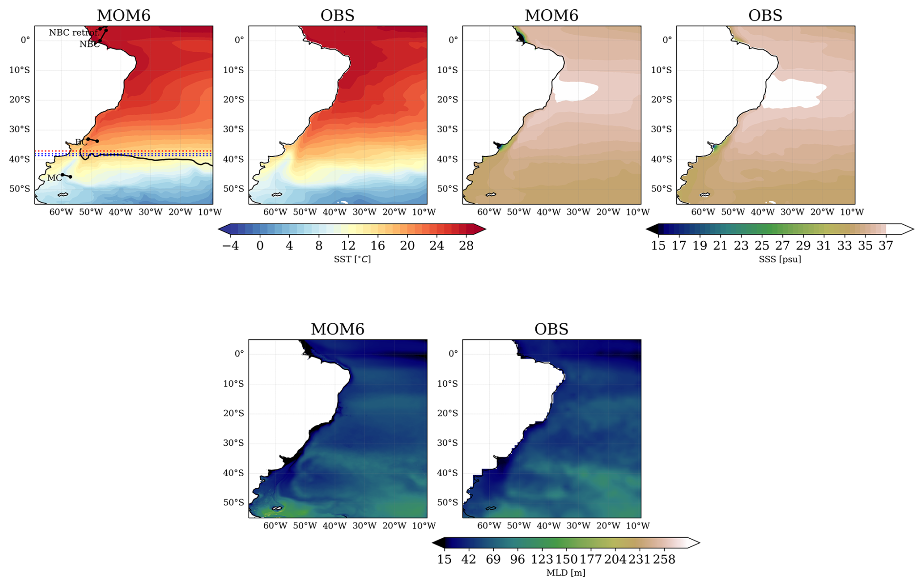
Figure 2 Sea Surface Temperature (top row), Salinity (middle row), and Mixed Layer Depth (bottom row), 20 year mean from the simulation (left) and WOA observations (right). In (a), the illustrated black line is the 10 °C isotherm at 200 m, where it meets with the 1000 m isobath, an estimate proposed by Garzoli and Bianchi (1987) to indicate the BMC separation in the model. The dotted curves represent the mean BMC separation using (red) GLORYS12v1 reanalysis and (blue) the obtained from satellite observational sets by Goni et al. (2011).

The model captures the development of the BMC, with the location of the temperature gradients in the region. The northward propagation of surface cold waters through the MC ends at approximately 37° S. The confluence with the BC appears within this region, which is close to estimates from observational data (Fig. 1; Goni et al., 2011; Lumpkin and Garzoli, 2011). A similar gradient is found in the observations, but cooler temperatures emerge near the La Plata Basin coast.

The model shows extra fresher waters near the La Plata and the Amazon Basins, indicating that the salinity is close to zero downstream of the basins. The model presents less salty waters than the observations at around 10–20° S, which appears to be related to the river discharges. However, the freshwater inputs look trapped in shallower depths on the coastline, and according to the ocean circulation (Fig. 1), the fresher water inputs flow south for the La Plata River and northwest for the Amazon River. The MLD pattern diagnosed by the ePBL's model scheme is consistent with the patterns of the observations despite the impacts of the river on the coastline circulation.

Contrasting patterns between the shallow and deepest regions appear from comparing the model seasonal averages with reanalysis from GLORYS12v1 with similar horizontal resolution (Jean-Michel et al., 2021). Figure 3 shows the sea surface density for each trimester, estimated by the equation of state for ocean models considering temperature and salinity (Wright, 1997). There is a higher consistency in the seasonal density between the fields far from the coast. Some differences in temperature contours emerge in the northwestern and southwestern South Atlantic, where the model keeps colder equatorial waters during most seasons. Although the difference in the temperature field has maximum values of −1 °C to the south of 30° S, especially during March to May (MAM) and June to August (JJA), it reproduces a weaker variance in the density field. The difference in density in the tropics is unrelated to the temperature variations and indicates the presence of freshwater inputs from the rivers, as indicated in Fig. 2.

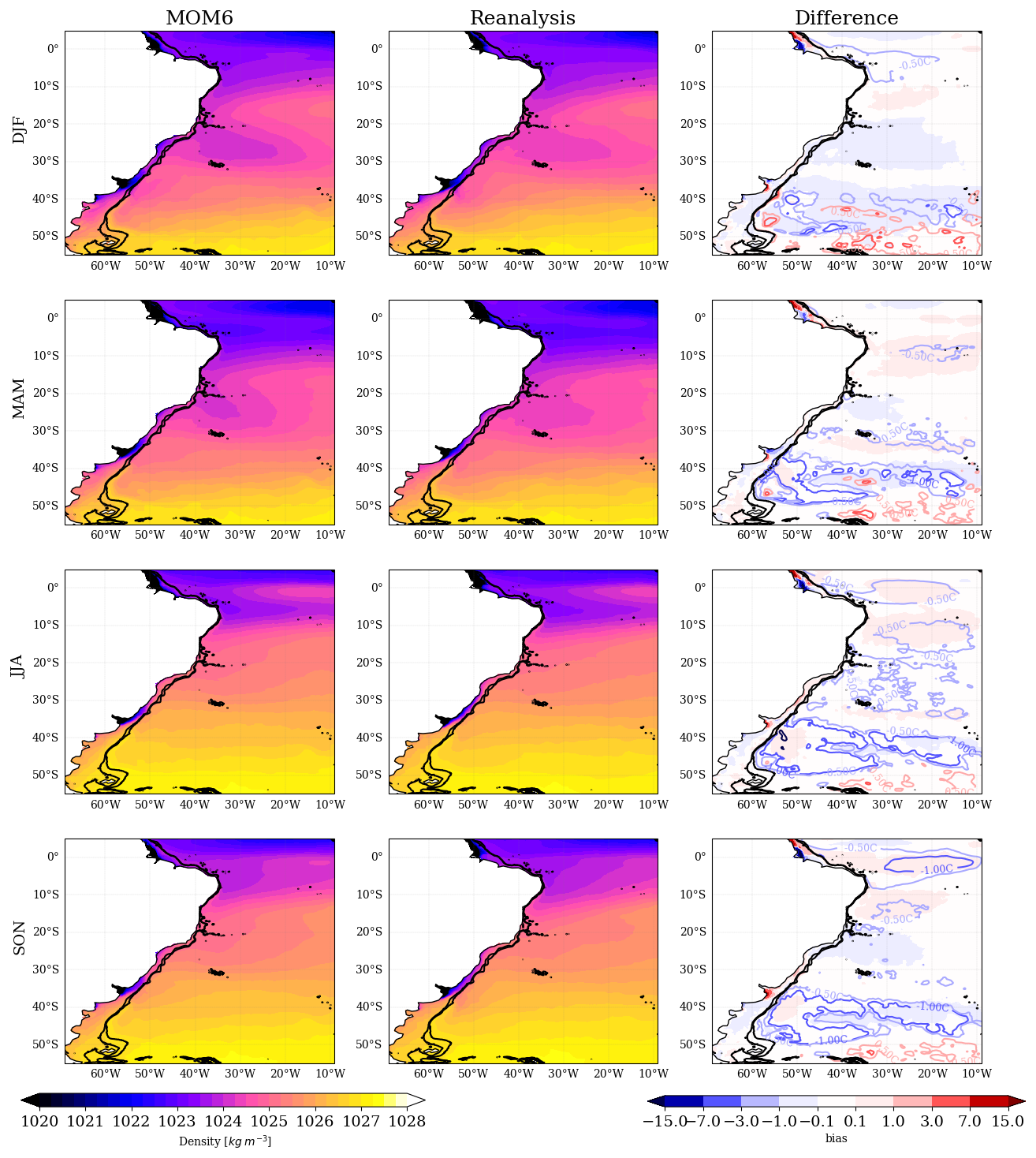
Figure 3 Seasonal mean surface density for the MOM6 simulation, the reanalysis (GLORYS12v1) and error. Each row shows a season, from the top to the bottom, DJF, MAM, JJA, and SON, marking the transition from austral summer to spring. The means consider the period from 1997 until 2017. The contours in the right column show the temperature errors in the open ocean (depth ≥1000 m), with contours at ±0.5, 1.0, and 3.0 °C. The thick black contours indicate the 200 and 1000 m isobaths.

The most significant differences in density appear in the shallow areas in the Amazon region, which exhibits variability related to the river's seasonality. The contrasting heavy rainfall related to the ITCZ displacement is related to the region's variability (Valerio et al., 2021). It contributes significantly to the mean flow from December to February (DJF) until MAM, with fewer discharges during JJA and September to November (SON). The difference in the density fields (Fig. 3) indicates that the model representation of the river discharges is more coherent during MAM, the period of higher freshwater discharge. The model's salinity distribution is counterbalanced in the other drier seasons, showing reduced salinity in the Amazon River basin and increased in the extreme northwest of the domain. Thus, deviations in the mixing of the river discharges imply the appearance of a core of higher density northwest of the domain and a lower density in the Amazon basin in Fig. 3. The density is higher in the model when more saline waters than the reanalysis are found and lower when more fresher waters appear.

Like the Amazon, the river seasonality implies modifications in the river discharges in the La Plata Basin. The model overestimates the density downstream of the La Plata Basin due to more saline waters on the southwest coast, mostly during SON. During winter (JJA), strong runoff is enabled by the frequent passage of atmospheric systems when the intense rainfall and wind spread the freshwater discharges of the river plume (Campos et al., 2013; Lago et al., 2019; Piola et al., 2005).

The importance of determining the advancement of freshwater plumes into the open ocean in both basins has been described in the literature (Valerio et al., 2021; Campos et al., 2013). Although the surface fields based on the 20 year model averages exhibited bias constrained by the coastline, the freshwater plumes accurately display the river seasonality. The river discharges simulated by the model represent the impact on the MLD seen in Fig. 2. In addition, the salinity variations near the Amazon and La Plata basins also considerably impact the surface density comparable to the reanalysis (Fig. 3). Although a similar resolution increases the consistency of the results in the basins, unbalanced freshwater amounts still occur. The results indicate that the amount of freshwater on the surface and the lower density contribute to less mixing in shallower depths. At higher depths, the similarity of the results, especially in MLD and density patterns, indicates that the unbalanced freshwater influences the appearance of local biases more strongly at the deltas of the Amazon and La Plata Rivers. However, there are still biases near the BMC and in tropical regions that may be due to other factors.

3.2 Vertical Structure of Temperature and Seasonal Variability

Profiles of potential temperature in Fig. 4 characterize the vertical structure in the ocean model against the reanalysis and the PIRATA buoys observations. The depth of the 18 °C isotherm compared to the buoys evidences the conformity in the vertical structure. The 18 °C isotherm in the A and B observations shows deeper seasonal fluctuations during SON, so the model fails in reproducing the structure. During the warmer season, MAM, when the warmer waters reach deeper layers in the observations, the model remains cooler until the wintertime. This effect reduces the MLD in the model, which shows a 30 m shallower MLD (Fig. 4, right column) than the other datasets in the buoy sites (Fig. 4, left and center). The difference is even more critical at the buoy B site, where the MLD is more than 30 m shallower in the model.

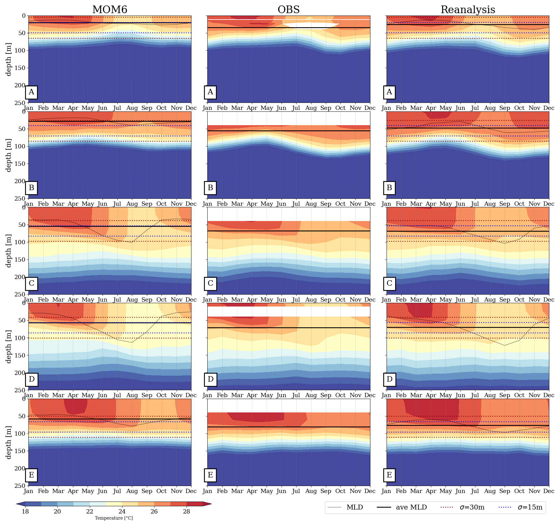
Figure 4 Mean annual cycle of the vertical profile of temperature and MLD at PIRATA buoy sites. The colors display the temperature, and the lines are the MLD. The letters identify the buoy sites from A to E. MOM6 outputs are on the left column, observed data from the PIRATA buoys are in the center, and reanalysis products are on the right. The MLD for observation and reanalysis are estimated with the ΔT=0.2 °C temperature threshold from a near-surface value and the 10 m. Missing data appears at different depths in the observations and are shown in white. The dashed lines highlight depths above/below the mean buoy-estimated MLD in blue with a difference of 15 m and in red 30 m.

The temperature at shallow and deeper regions shown at the buoy sites in Fig. 5 explains the reduced heat entrainment from the surface layers in the model due to different factors. Near the surface, the model temperature is approximately ≤1 °C lower than the reanalysis and the buoys through the seasons (Figs. 3 and 5a). The model presents a well-defined seasonal cycle near the surface (Fig. 5a), when a warmer surface appears during MAM and cooler in JJA and SON. More contrasting outliers are in the 80 m depth layer (Fig. 5b), with the buoys in the tropical region revealing higher temperatures obtained with the hybrid coordinate compared to the z^∗ coordinate. In the other buoy sites (C, D, and E), far from the equatorial region where the water column is deeper (Fig. 1), the model presents a reduced bias. Reproducing the 80 m temperature in the equatorial region is a challenge even in the reanalysis (Fig. 5b). Compared to the model in z^∗, the observations at sites A and B present 2 °C warmer temperatures during SON and 1 °C warmer temperatures during DJF. This divergence for site B starts in JJA, getting colder by more than 2 °C than the observations in SON. For buoy A, the most divergent seasons are SON and DJF.

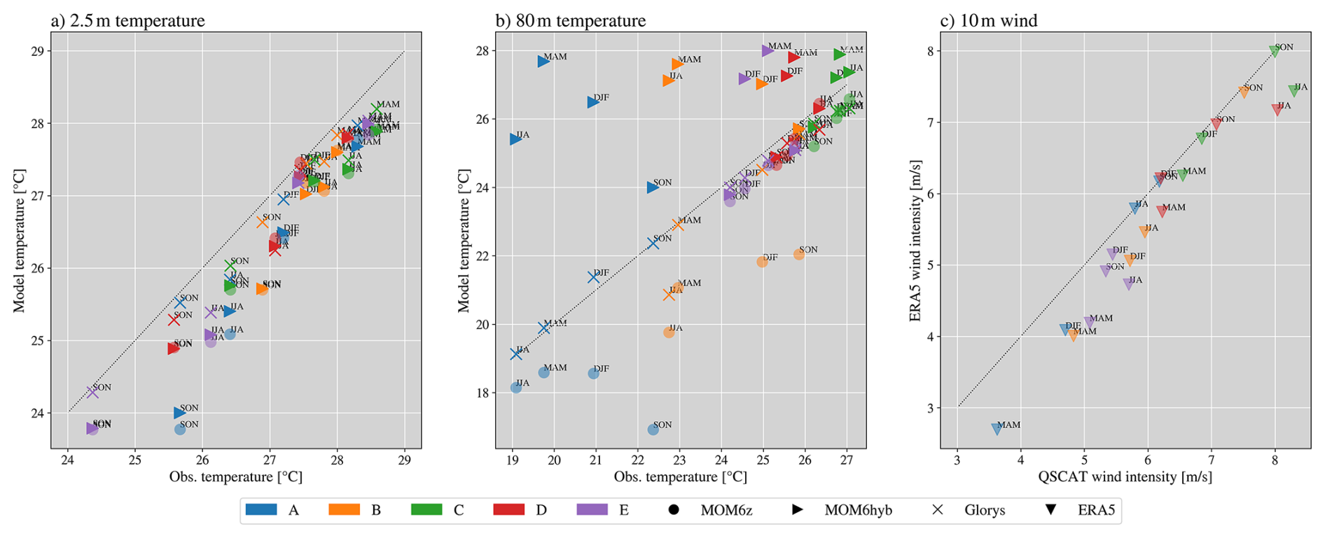
Figure 5 Seasonal 2.5 and 80 m temperatures and 10 m winds, compared against observations. The graphs display the temperature at 2.5 m (a) and 80 m (b) for the model and reanalysis compared to PIRATE buoy observations. In (c), the atmospheric forcing for the model, 10 m wind from ERA5, compared to QSCAT satellite observation (Hoffman and Leidner, 2005). Colors distinguish the buoy sites from A to E. The model data is plotted with two vertical discretizations: MOM6z takes the z coordinate system and MOM6hyb uses a hybrid system. The same period of 5 years is considered for the model data. The reanalysis from GLORYS12v1 is marked with crosses and ERA5 triangles. The seasons are named as DJF, MAM, JJA, and SON.

The heat entrainment capability of the model in the equatorial region is enhanced by changing the vertical coordinate from z^∗ to the hybrid coordinate. This is shown by comparisons of the z^∗ and hybrid coordinates for the 5 year run (Fig. 5b). This vertical discretization allows the warmer structure at 80 m to be reproduced on SON, although the temperatures in other seasons remain high. A more qualified description of these mechanisms and additional adjustments can be disclosed in the following studies. For comparison, Fig. A1 in the Appendix shows that the temperature distribution remains the same for the model in the z^∗ coordinate over the entire simulation period.

The tendency of the model to underestimate the entrainment of seasonal heat at the equator indicates a concern about the ITCZ displacement. The latitudinal ITCZ displacement causes the most intensive surface heating during MAM (Valerio et al., 2021), reproduced with lower bias by the model considering observations (Figs. 3 and 5a). This enables the development of stratification and heating of the deeper layer in the following seasons. However, although the model reproduces the warmer temperatures during MAM and JJA, the deeper layers remain cooler until SON (Fig. 5b). This deviation indicates that although the model receives the seasonal heat at the surface, it gets under-mixed during the stratified period. In contrast, for the reanalysis and the hybrid MOM6 set-up to reproduce the heating and the accordant stratification structure during SON, the 80 m-depth waters are slightly warmer than the buoys for sites A and B.

The seasonal ITCZ displacement impacts wind speed in the buoy sites, which is a misleading diagnostic that can interfere with ocean currents and mixing. The model wind forcing (ERA5) is compared to QSCAT satellite observations in Fig. 5c to observe this effect. Although the ITCZ depends most on the wind structure during DJF and MAM in the equatorial region, ERA5 wind is slower than the observations through all seasons. During the warm season, buoy sites A, B, and E present wind forcing almost 1 m s⁻¹ slower. The wind pattern, which contributes to the vertical mixing, suggests that equatorial region temperature biases occur due to the lack of a wind-driven source.

The deviation of mixing temperature and freshwater in the adjacent layers can be a response to the vertical coordinate system (Fig. 5b) and to the weaker ERA5 10 m-wind, compared to the estimates from satellite observations (Fig. 5c). The winds lead to less mixing in the bottom layers since it dissipates the wind stress, the main energy source to the currents, and subsequent horizontal transport. These factors can also contribute to the salinity differences in the northwestern part of the domain. Lighter density is placed in the Amazon Basin due to the weak zonal winds and a lack of mixing, resulting in the fresher water patterns in the surface. In turn, the lack of advection of freshwater results in salty and more dense waters (>7 kg m⁻³) in the northwest corner of the domain (Fig. 3).

3.3 Meso- and Large-scale Circulation

The ocean circulation comprises the distribution of the current speeds and energy, potentially related to the tracer exchanges in the domain. The analysis in this study allows the observation of meso- and large-scale circulation as represented by the model. The 20 year mean surface current speed model outputs in Fig. 6a display the mean natural path of the main currents, depicted in Fig. 1: SEC, NBC, BC, and the MC, distinguished from the mean flow. The BC is observed through the warm high-speed currents on the mid-western Atlantic flowing southward from 20° S. The MC surrounds the east of the Patagonian Shelf on the Argentinean coast south of 40° S, and the eastward flow in 50° S marks the origin of the South Atlantic Current. The mean speed field also allows the appearance of high-speed currents in the BMC, between 35 and 45° S. In the northwest, the flow of the NBC and the connection with the SEC is also pronounced. The NBC is north of 5° N and to the northwest. Thus, the model places the ocean currents that agree with the general location described by others (Lumpkin and Garzoli, 2005; Oliveira et al., 2009).

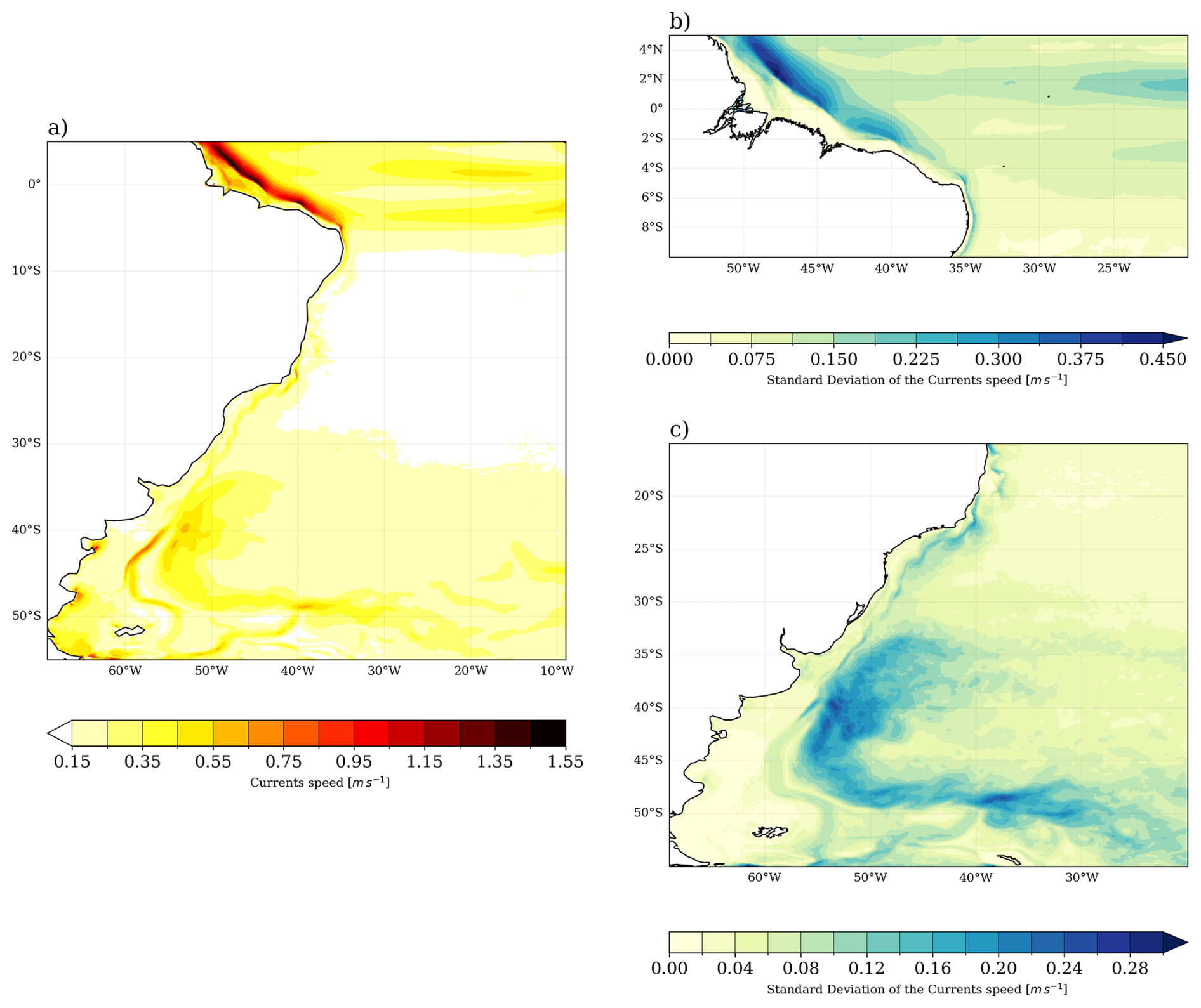
Figure 6 Mean sea surface currents (m s⁻¹) (a) and standard deviation of the mean speed (m s⁻¹) for the NBC (b) and the BMC (c) regions. The standard deviation considers the monthly variability of speed in the domain. The main BC and MC path appears with currents speed above 0.3 and 0.6 m s⁻¹, respectively, while the speed of the NBC is above 1 m s⁻¹.

The current speed standard deviation for the two main WBCs reveals that the model can reproduce the variability of these features in various different shallow parts of the domain (Fig. 6b and c). The NBC is the most prominent current in the domain, and the speed reaching 1.5 m s⁻¹ and the standard deviation of 0.45 m s⁻¹ indicate larger variability. This dynamic background induces the formation of mesoscale structures through the NBC retroflection (Bueno et al., 2022; Garzoli et al., 2004). Part of this variability is due to the topographic gradient but also induced by the seasonal cycle and the river discharges of the Amazon River. Another contributing factor is the SEC's high speed (>0.45 m s⁻¹) and deviation (>0.15 m s⁻¹) in equatorial waters. The SEC maintains East-West oceanic transport, suffering from the seasonal effect drift due to the trade winds, which decreases its intensity during DJF compared to JJA (Lumpkin and Garzoli, 2005). The propagation of mesoscale eddies also induces the intense variability noted near the BMC. The high speed and deviation are constraints in an area where the retroflection of the MC propagates eddies to the west. This region is known for the shelf-break upwelling, where the significant depth gradient and the proximity to the MC contribute to the enhanced mixing and upwelling (Fig. 1).

The presence of eddies relates to the transference from mean potential to mean kinetic energy, observed by the Sea Surface Height (SSH) variability and MKE in Fig. 7. The MKE pattern displays the highest values where the highest speed is placed, as expected for both WBCs, but the variability in the SSH is observed only in the BMC (Fig. 7d). The high-resolution benefits the maintenance of the MKE distribution, particularly in the BMC, where the eddies are the major variability driver. To the west of 55° W, the Patagonian Shelf circulation is guided by the interaction of semidiurnal and diurnal tidal components with the bottom friction and wind stress (Palma et al., 2004, 2008). The speed of the currents in the southern Patagonian Shelf in the model output represents this dynamical effect (Fig. 6a). In other parts of the domain, the variability in the SSH is higher only in the river mouth. This indicates the influence of barotropic tides, which intensely modify the SSH in shallower regions. The MKE distribution and intensity of >0.2m² s⁻² are similar to observations (Oliveira et al., 2009), and the distribution agrees with reanalysis (Poli et al., 2022). The high variability in the BMC occurs due to the physical processes related to the confluence of the BC and MC, which, near the Patagonian shelf, promote eddy formation due to the continental slope. As it shows fewer SSH deviations, the propagation of eddies in the NBC in this simulation is reduced. This suggests that the energy cascade primary process may not only drive eddy formation in this region but also other physical dissipative processes. The distinguished aspects found for the NBC and the BMC are covered in different sections in the following chapter, where this study evaluated the seasonal variability and trends.

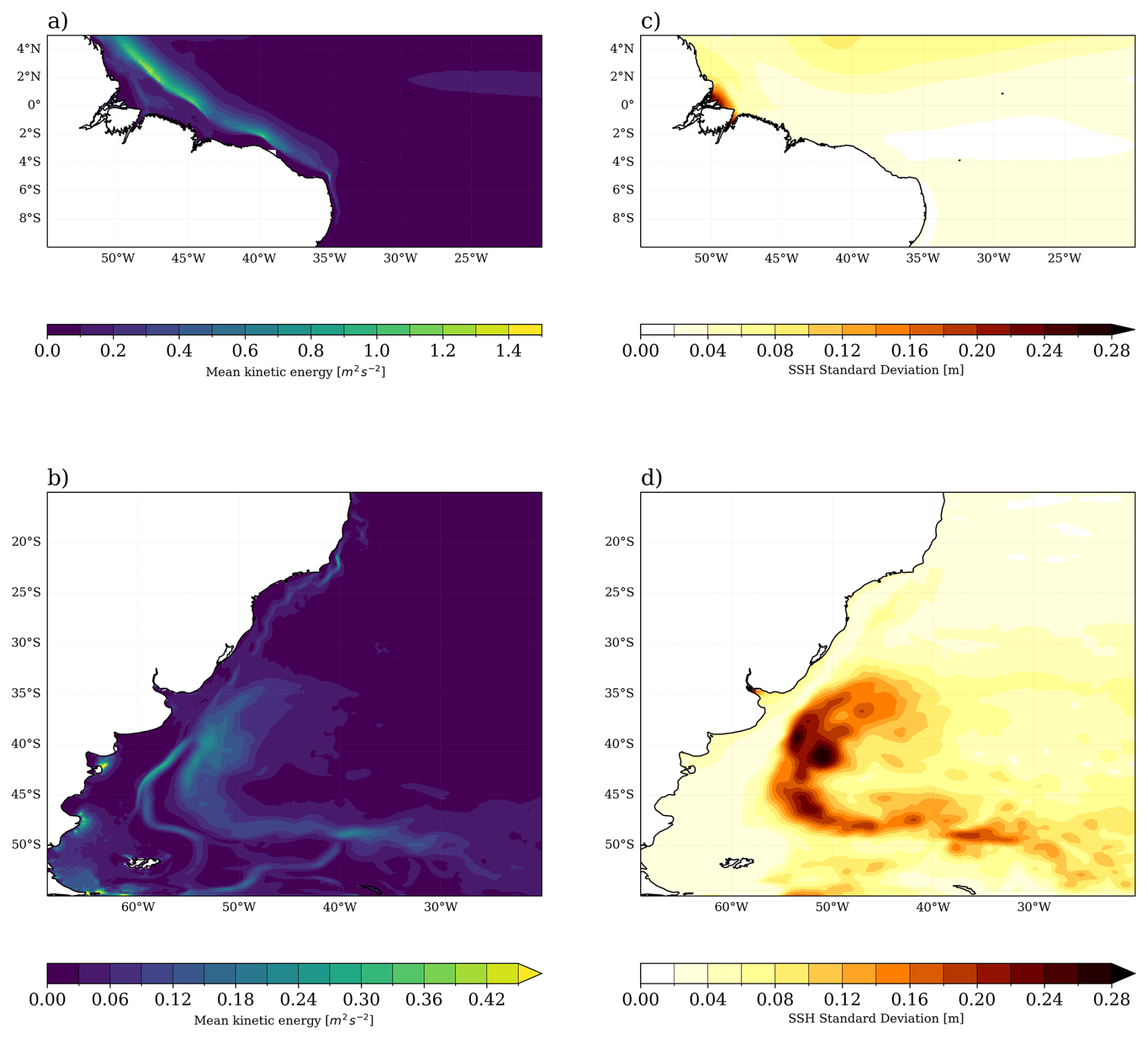
Figure 7 Standard deviations of the Mean Kinetic Energy (m² s⁻²) (a, b) and SSH (m) (c, d) in the regions of the WBCs. In the latter, fields are std concerning the monthly variability from 1997 until 2017.

4 Seasonal Variability and Trends of the WBCs

4.1 Brazil-Malvinas Confluence

The high variability in the BMC occurs due to the physical processes related to the confluence of the BC and MC, which, near the Patagonian shelf, promote eddy formation due to the continental slope (Oliveira et al., 2009). Mesoscale variability and eddy propagation are often diagnosed from the SSH standard deviation (Fig. 6). The model patterns show consistency with those analyzed by Oliveira et al. (2009), using observed data from drifting buoys interpolated onto a 0.5°×0.5° grid. The model also shows similarity with the observed MKE field from other studies (Oliveira et al., 2009; Combes and Matano, 2014a) (Fig. 7). Several authors have emphasized the importance of wind stress in maintaining the barotropic component of the circulation of the northern Patagonian Shelf (Lago et al., 2019; Campos et al., 2013; Palma et al., 2008, 2004; Combes and Matano, 2018). The most prominent influence is during the well-mixed period (JJAS) rather than in the stratified period (JFMA), when the baroclinic component is more relevant (Lago et al., 2019). This effect can be diagnosed in the climatological field in Fig. 7. The presence of eddies in the annual average enhances the standard deviation of SSH and reveals the baroclinic component. The barotropic component is related to the total MKE distribution in the annual average in Fig. 7c. It is confirmed that the main variability of the velocity fields is related to eddy propagation, which drives the SSH variability. The model consistently preserves the circulation features of the BMC even in regions close to shallow shelves.

The model captures the seasonal behavior of the BC and the MC, revealing the density variations through the seasons in Fig. 3. This implies that the MC takes a northern place during the colder seasons in this hemisphere (JJA, SON) while the BC advances during the warmer seasons (DJF, MAM). This is also evident in the seasonal cycle of the BC and MC transport (Fig. 8) and in the number of extremes per season (Fig. 10). The model registered below-average transport for the MC from October through April and above-average transport from May through September. The BC has the opposite cycle, and above-average southward transport occurs from December until April. The seasonal cycle is similar to what was found by Combes and Matano (2014b) with ROMS simulations. Despite this, ROMS presents a higher MC mean transport of around 73.1 Sv at 41° S compared to MOM6's 60.3 Sv transport at 45° S (Fig. 8). The BC transport is higher in this simulation, around 57.9 Sv, while ROMS registers 40 Sv at 33° S.

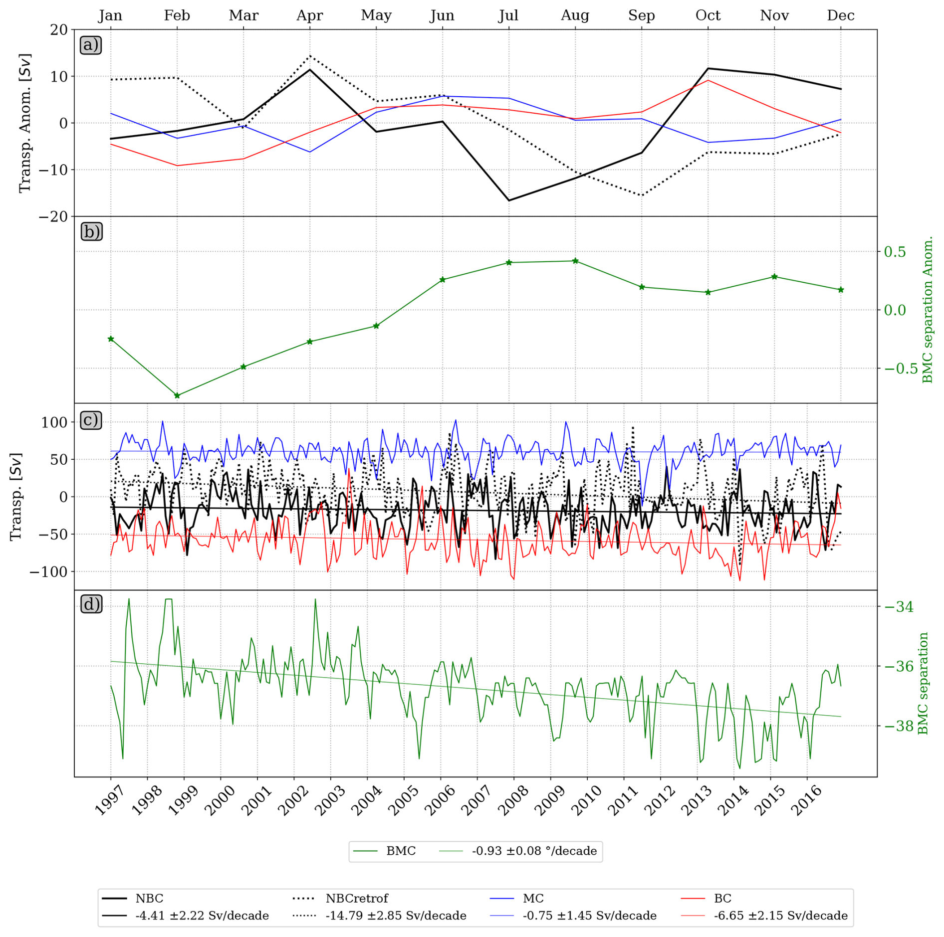
Figure 8 Ocean transport of the WBCs in the domain and the latitudinal displacement of the BMC separation. The first row shows the mean monthly transport anomalies for each WBC, and the second row shows the mean monthly BMC separation anomalies. The third row depicts the interannual transport for the WBC, and the bottom row shows the BMC positioning. The ocean transport is vertically integrated between latitudes 0° and 3.5° N for the NBC and 4 and 5° N for its retroflection, whereas it is at latitudes 45 and 33° S for the MC and BC, respectively. The transects are depicted in Fig. 2. The positive transport flows northward and east, and the negative transport flows south and west.

The transport of the BC and MC shows a high interannual variability, as depicted in Fig. 8. They can widely vary their transport from 10 to 88 Sv, with smaller transport in the BC (Goni et al., 2011). The increased MC transport induces the seasonal negative temperature bias in the 20 year mean temperature patterns from MAM until SON (Fig. 3). Besides, the transports show a negative trend, more than 10 times higher than the trend obtained with observations (Goni et al., 2011). This could imply a systematic error in the simulation. Studies indicated that adjustments in the model bottom friction modify the mean northern ACC transport, inducing changes in the mean BMC (Combes and Matano, 2014a; Peterson, 1992; Combes and Matano, 2014b). As in this simulation, the ACC transport is given through reanalysis data, the bottom friction is the parameter that could interfere with the MC variability. However, the BC offers a balanced higher southward trend, which other studies have indicated as a consequence of Atlantic Ocean warming (Lumpkin and Garzoli, 2011; Risaro et al., 2022).

Although the BMC separation occurs on average between the latitudes 37 and 39° S (Goni et al., 2011), several studies have recorded climatic trends of a southward shift in the BMC position. The trend is induced by the intense warming observed in this ocean (Risaro et al., 2022; Franco et al., 2020), but the intensity of this relation and variability is still uncertain. According to Goni et al. (2011), with satellite observations, this trend has a rate of 1.5° per decade between 1993–2008. Lumpkin and Garzoli (2011) indicated a varying rate between 0.6 to 0.9° per decade with data from 1992 until 2007. A numerical model used by Combes and Matano (2014b) revealed a displacement of 0.62° per decade, which the study related to the weakening of the ACC.

The BMC separation obtained from model outputs is the latitude where the 1000 m isobath meets the 10 °C isotherm at 200 m, which, according to Garzoli and Bianchi (1987), depicts a location of enhanced time-space variability of the front separation. For the 20 year MOM6 simulation, the mean BMC separation is at 36.76 ± 0.77° S, as depicted in Fig. 2. The plot shows the mean position obtained with GLORYS12v1 for the same period and by Goni et al. (2011), which considered satellite observations from 1993 until 2008. The model simulation is slightly (≈1°) more northerly than the other estimates in the plot. Using ROMS, Combes and Matano (2014b) estimate that the BMC separation is ≈2° farther south, around 39° S. The same reanalysis from GLORYS12v1 has been used in other studies have depicted a similar BMC separation near 38° S (Artana et al., 2019, 2021).

The 20 year simulation outputs allow for the characterization of trends in this ocean, which is important for diagnosing the variability of the mean state. The model overestimated the BMC separation trend over the years compared to observations. The simulation registers a −0.93° per decade deviation, while Goni et al. (2011) obtained different results based on observations of SST and SSH, with values of −0.39 and −0.81° per decade, respectively. Lumpkin and Garzoli (2011) indicate a trend between 0.6 and 0.9° per decade for 1992–2007. Despite the higher trend, the model mean BMC separation is close to other estimates (Fig. 2), indicating that the model seasonal bias is compensated and the MC positioning is stable in this simulation.

The trends of surface variables in Fig. 9 depict important patterns in the BMC region. The temperature in the BMC is very similar to the pattern obtained with satellite observations for the 1982–2017 period (Risaro et al., 20202). The temperature is warmer in most BMC vicinities, while it is cooler in the southern part of the domain, representing more than 0.5 std. Enhancing the polar northward flow from the Drake Passage contributes to the negative SST and SSS trend, resulting in fresher and colder waters. In the BMC region, surface speed trends present a similar pattern; accordingly, warmer and saltier waters are faster and have increased transport, while colder and fresher waters are slower. This agrees with the number of BMC separation location extremes in Fig. 10, which reduces significantly through the years, confirming the southward movement. In a warmer environment, the transport generated by the BMC presents stronger initial energy, but its track has a southward displacement.

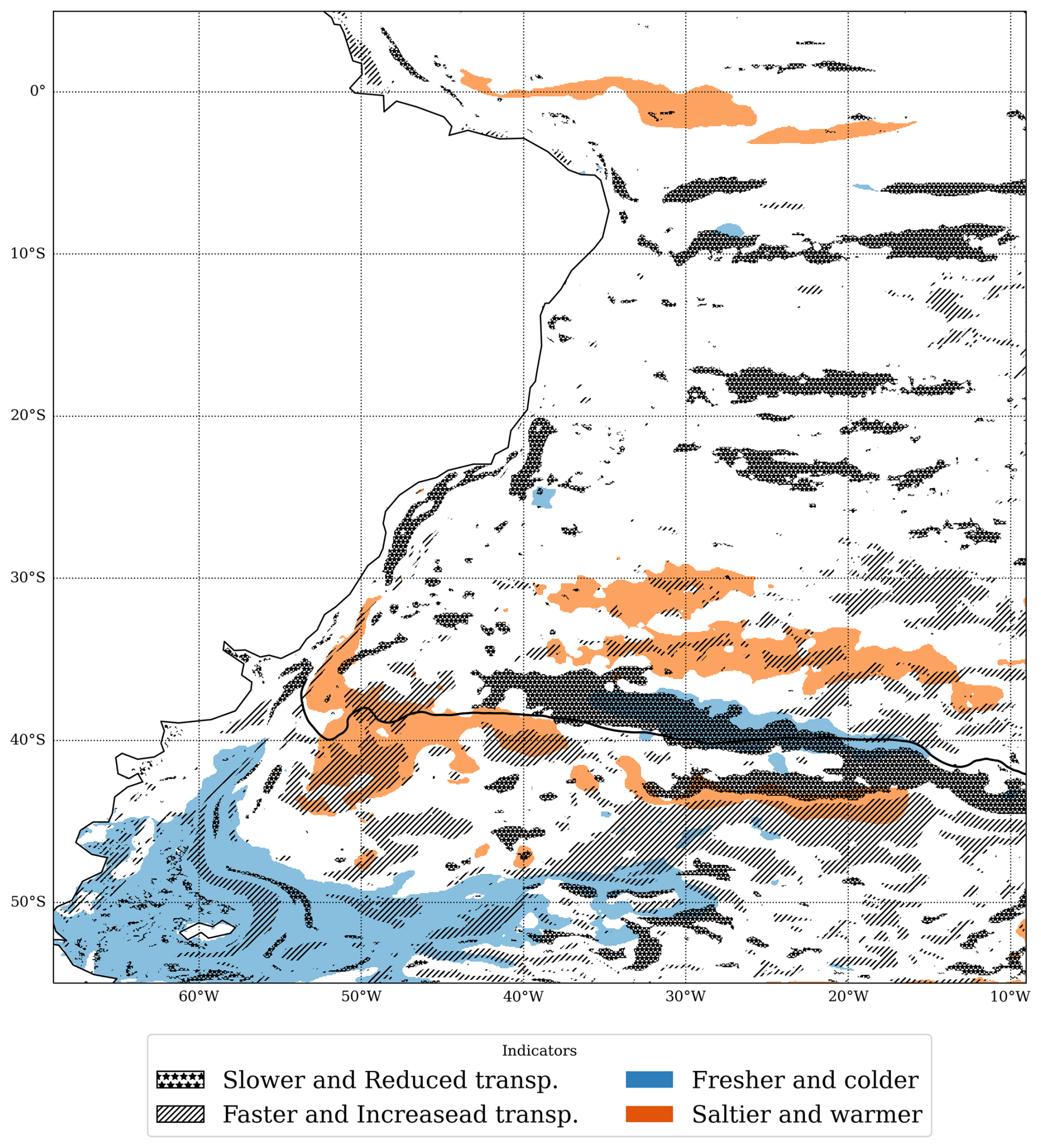
Figure 9 Trends in the WBCs. Trends of different surface variables simulated by the model. Trends originate from a 36 month running mean smothered series of standardized anomalies (Risaro et al., 2022). Colored regions are significant at a 95 % confidence level, according to Mann-Kendall's test (Mann, 1945; Kendall, 1975). The trends by decade are normalized, and the colors display anomalous patterns above 0.5 std.

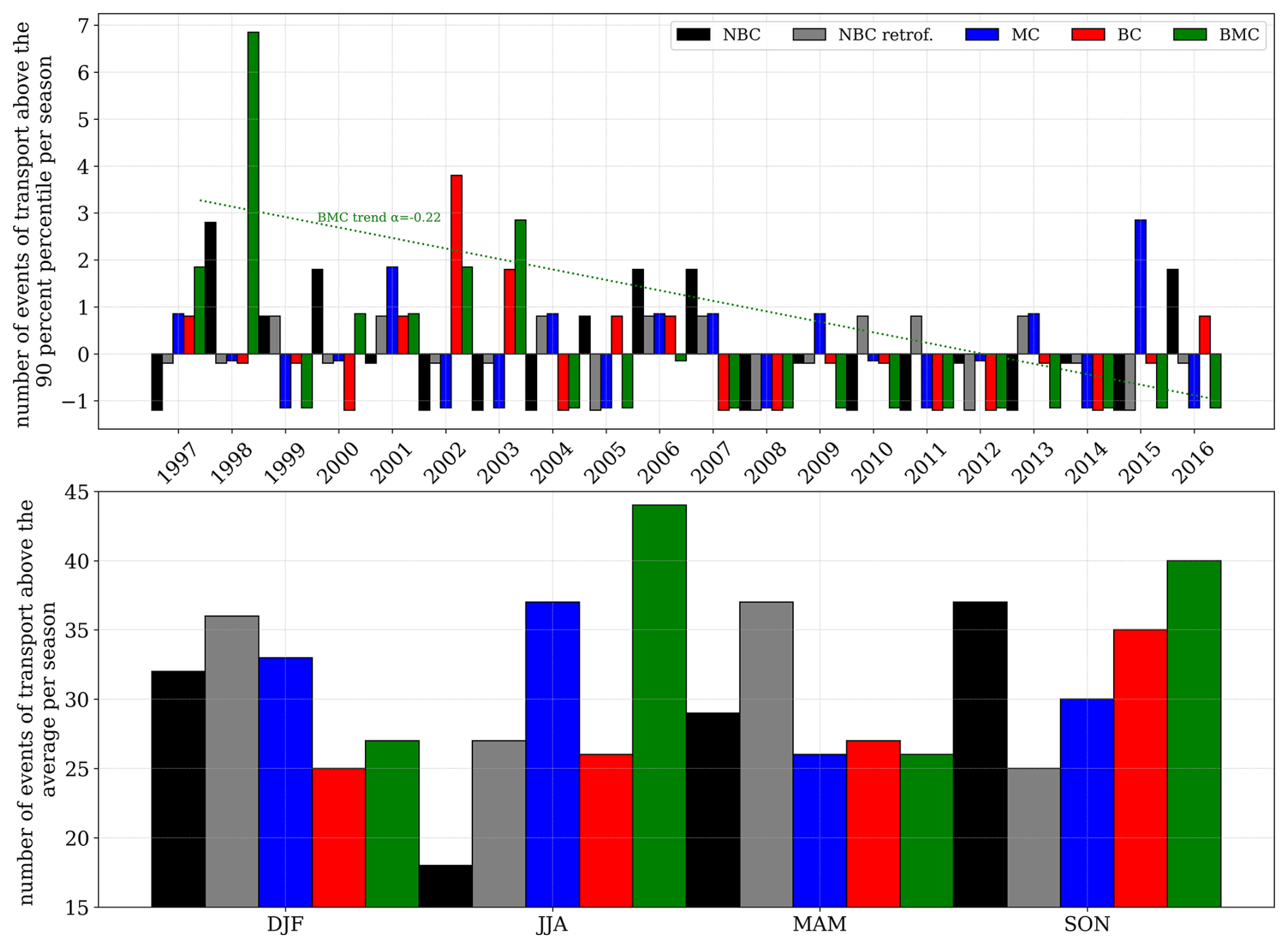
Figure 10 Registries of extreme transport events in the WBCs. The graphics show the events from 1997 to 2016 with transport above the 90 percent percentile per year (top) and above the average per season (bottom).

Concerning the patterns far from the coast, there is a warming longitudinal trend pattern at 35° S extending from 35 until 15° W, evident in the model but not in the observations (Risaro et al., 2022). The region is known for its constant westward flow and propagation of eddy from the Agulhas Current (Guerra et al., 2018). This indicates an intensification of the transport to the north of 35° S in comparison to what is observed farther south.

4.2 North Brazil Current

The NBC presents high variability associated with the propagation of eddies (Bueno et al., 2022; Garzoli et al., 2004). The model, however, underestimates the SSH variability in the NBC retroflection, which suggests there is weaker transport from the SEC to the NBC. Some authors use zonal transport estimates based on NBC propagation and retroflection sections to verify this diagnosis (Garzoli et al., 2004). The region is marked by intense currents, registering transport of 16 ± 2 Sv for the NBC and 22 ± 2 Sv for the retroflection obtained by Garzoli et al. (2004). Accordingly, the estimates for the same sections with MOM6 outputs indicate that the 20 year average transport is around 18.4 Sv for the NBC. For its retroflection, however, the transport series initiated with an amount of 22 Sv but indicated an average of 5.9 Sv (Fig. 8). Garzoli et al. (2004) considered a 15 month mean by local sounders measurements, registering a seasonal cycle with more intense transport during ASO, less intense during MAM for the NBC, and the opposite for its retroflection. The MOM6 simulation fails to reproduce any of these characteristics for the retroflection (Fig. 8a).

With a maximum latitude at 5° N, the simulation in this domain cannot fully develop the NBC retroflection and its eddies as its natural path can deviate from 4 to 8° N (Bueno et al., 2022; Valerio et al., 2021). The negative trend of the NBC retroflection reveals that NBC reduced its transport in the model, but it also indicates that its path has deviated over the years and moved outside the model's domain. Despite that, features like temperature, salinity, and transport of the currents in the NBC and tropical region are precisely described during MAM. The bias appearing during JJA is maintained through the colder seasons (Fig. 3). This indicates a lack of mixing, which can be either due to the influence of the wind speed (Fig. 5c) or the use of a z coordinate vertical structure (Fig. 5b). Interactions of the winds and the currents are important for mixing and eddy kinetic energy supply (Song et al., 2020). Thus, insufficient winds could reduce eddy formation, reducing the seasonal NBC retroflection transport.

Although this simulation cannot fully represent the development of the NBC retroflection, investigating this deviation is crucial to determine the variability of some climate patterns in the equatorial region, such as the storm track, the AMOC, and the ITCZ. The absence of eddy propagation (Fig. 7) and transport (Fig. 8) in the region, for instance, might indicate deviation in the dynamical structure of the model. Nevertheless, the model conserves large-scale SEC transport since the mean NBC eastward transport resembles values slightly closer than those obtained from local measurements (Garzoli et al., 2004). Still, many other factors could disfavor the propagation of NBC eddies. The proximity to the northern boundary is a critical limiting factor, since this front could change its position through the years. However, it is also important to indicate that the negative trend observed in the region can be related to atmospheric mechanisms and trends.

The trends in Tropical Atlantic Ocean waters indicate elevated temperature and salinity, as shown in Fig. 9. This trend is not associated with transport and speed patterns. The Amazon River flow increases the transport and current speed in the northwestern part of the domain. The merged patterns of current speed and transport attenuate the eccentricity of the currents in the region, as revealed in Fig. 8b. Thus, while the NBC and its retroflection experience a reduction in transport, they exhibit an increase in speed. The lack of stratification, as shown in Fig. 4, suggests an inefficient transport of momentum to the sub-surface layers. This may also be influenced by external forcings or the redistribution of flow pathways out of the domain.

4.3 Evaluation of external and internal forcings

The WBCs in the Southwestern Atlantic domain feature intense variability and trends. This has been indicated by trends in the mean state of the surface variables (Fig. 9), along with a tendency toward reduced extreme transport (Fig. 10). Furthermore, extreme transports in the BC/MC are associated with the displacement of the BMC. In 1998, a year of an elevated number of extreme BMC displacements, the signal that enhances the southward movement of the BMC is unrelated to the transport amount toward the region. Thus, external teleconnections also generate modulations of the currents in the region. This section further investigates the components of this modulation.

External forcing, such as atmospheric teleconnections, can explain the mixed signals of the trend, indicating that the influence is not driven strictly by local forcings. Combes and Matano (2018) observed that the La Plata Basin flows are linked to the interannual variability of the ENSO. The correlation coefficients between the WBCs and climate indices indicate the susceptibility of the MC to Eastern Pacific Ocean variability, with significant correlation between its transport and the Nino1.2 and the PDO indices of 0.14 and 0.18, respectively. The BMC also presents a significant correlation of 0.26 with the Nino1.2 index (NOAA, 2024). These relations combine tropical and extratropical teleconnections with atmospheric components that drive turbulence and freshwater discharge in the domain (Combes and Matano, 2018), resulting in strong MC and northern BMC in response to rising temperatures in the Eastern Pacific.

Due to the proximity to the coastal slopes, the internal variability of the currents and transport in the WBCs results in a broader number of dynamic interactions, different from those in the open ocean (Hughes et al., 2019). The wave propagation from tropical regions in the Pacific follows the western South American coastline, which propagates and contributes to the coastal dynamics in the Southwest Atlantic Ocean. Poli et al. (2022) reveal that Kelvin wave dispersion and Rossby wave propagation from the Madden-Julian Oscillation are linked to the barotropic and baroclinic components of the coastal trapped waves in the Southwest Atlantic Ocean.

To examine the waves occurring on the coastline in the model outputs, we plot a dispersion diagram following Wheeler and Kiladis (1999). The diagram reveals the spectrum eccentricity of a determined location at a determined period in time, enabling the dynamic patterns to be classified by frequency and wavenumbers. Figure 11 displays the distinctive patterns during two distinct behaviors of the BMC separation: southern and northern extreme shifts. The wave patterns indicate that this region is influenced by coastal and open ocean dynamics. In the diagram, the low-frequency energy waves of positive and negative wavenumbers reveal the influence of eastward and westward Rossby wave propagation. This region is affected by westward waves that could be driven by MJO propagation (Poli et al., 2022), while the eastward waves are a response to the Indian Ocean Rossby Wave propagation from the Agulhas Current (Pontes and Menviel, 2024). Another important pattern is the higher-frequency modes, whose behavior is similar to that of inertial gravity waves, and its associate this pattern with the coastal trapped wave disturbance. Despite the high frequency, the inertial gravity waves in this region have shorter wavelengths. Their propagation is constrained in the region and is mainly interacting with the bottom topography, and with other wave patterns (Alford et al., 2016). The driver is sustained by local variations in density and temperature on the ocean surface due to wind forcing. The most important aspect of this pattern in the region is the interaction of inertial gravity waves with the mesoscale and submesoscale motions (Alford et al., 2016).

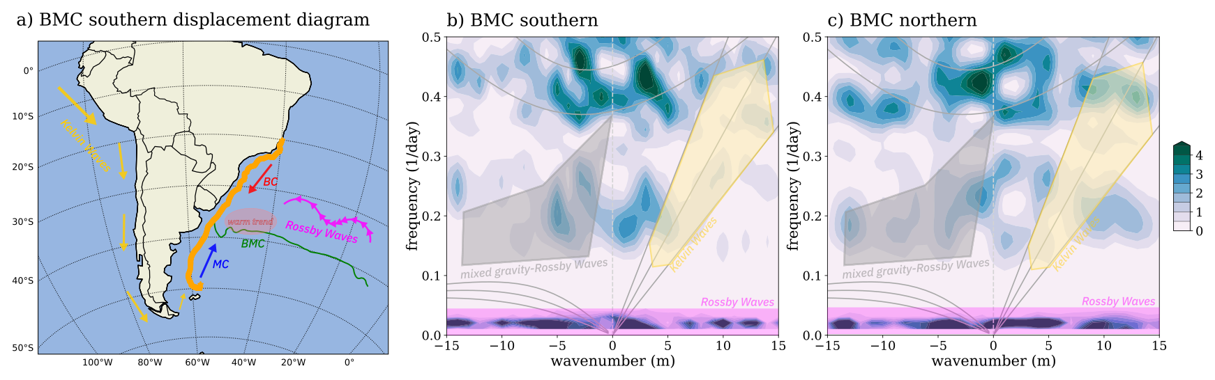
Figure 11 Diagram with the interactions in the BMC region modifying its displacement (a). Frequency and wavenumber diagram during extreme meridional displacement of the BMC separation: (b) BMC southern in 2014, (c) BMC northern in 1997. The spectrum reveals the frequency and wavenumber in the model SSH outputs band-pass series filtered between 40 and 130 d for the 300 m isobath between latitudes 20 and 50° S. The diagram is for the transect along the 300 m isobath, in orange.

Different energy spectra occur during the distinct events for mid-frequency waves, classified as mixed gravity-Rossby Waves and Kelvin Waves (Fig. 11, marked in grey and yellow). The propagation of Kelvin Waves also relates to external forcing from equatorial sources (Hughes et al., 2019; Poli et al., 2022). According to Poli et al. (2022), the MJO propagation trigger Kelvin Waves propagation in Central Pacific that reaches the South Atlantic driving coastal trapped waves into the Southwest Atlantic Ocean. This results in strong trigger for waves propagating northward (Poli et al., 2022), auxiliating the acceleration of the northern MC and northern BMC. The diagram confirms that coastal trapped waves energetic disturbance contributes to northern BMC displacement, which is presented here in response to rising temperatures in the Eastern Pacific. This result increases the understanding of the drivers of extreme shifts in the BMC separation.

5 Summary and Conclusions

This work analyzed the representation of the Southwestern Atlantic circulation using a 20 year MOM6 simulation at a 7 km resolution, focusing on the variability of the WBCs. The results first explore the performance of the simulation, which has proven to be skillful when compared to observational and reanalysis datasets. The Eddy-permitting resolution allows a better representation of the SST and SSS fields than coarser resolution simulations. The model accurately captured surface ocean circulation and temperature and salinity gradients. The maximum negative SST bias of 1.0 °C is sufficiently good performance for forecasting ocean conditions. The correspondence between density and MLD to the salinity and temperature structure indicates that the model reproduces thermodynamic effects fairly. Their effects on the density field drive the large-scale circulation, as highlighted by the global circulation and mesoscale features.

The transport of the currents in the simulation has evolved over decades in the Southwestern Atlantic WBCs. The BMC separation is a region with stronger kinetic energy in the domain. Observing the components of the BMC variability can help identify the location of eddy propagation and shelfbreak upwelling. Although it has been related to the bottom drag, the enhanced southward shift in the BMC is also consistent with the heating trend in this study. The warming Atlantic is followed by a modified BC transport with an increase of 6.65 ± 2.15 Sv in the southward flow per decade. This feature is usually balanced by the conservation of the MC transport. The trends show enhanced northward transport of fresher and colder waters from the ACC, which reduces the temperature by bringing cool waters to the region. Despite this, the trends modify the location of the BMC separation, with a southward displacement of 0.93 ± 0.08° per decade.

We show that the location of the BMC separation has extremes that relate to natural climate variability patterns in the Pacific Ocean. The Pacific Ocean warming has a stronger correlation and enhanced activity during MC transport extremes and northward BMC. The Nino1.2 (East Niño) and PDO indices corroborate this behavior. The impacts are explained by a spectral analysis, which reveals Rossby and Kelvin Wave-like disturbances, in addition to the inertial gravity waves intrinsic in the slope proximity. Eastward and westward propagating Rossby waves occur as a link between tropical disturbances such as the MJO and the Agulhas Current (Guerra et al., 2018; Poli et al., 2022). The Kelvin wave disturbances appear to be the main energy source for the BMC separation latitudinal shift, revealing strong spectral power for a northern BMC positioning as they propagate northward. This indicates that although the warmer Atlantic enhances the southward shift in the BMC separation, mechanisms intensified by the warmer Eastern Pacific can enhance the northward flow.

The NBC also presents reduced transport, but the model has captured a higher negative trend than that of the one in the BC. The unbalanced reduction of 14.79 ± 2.85 Sv per decade for its retroflection weakly correlates with natural climate variability patterns. Still, other contributing factors can explain the intense influences observed in the NBC activity. We found that the transport trends occur alongside a positive current speed trend. Since much of the variability of the ocean surface currents receives a direct contribution from the wind, weaker winds lead to reduced NBC eastward propagation with fewer eddies. Along with the absence of winds, we show a reduced stratification pattern commonly linked to lower temperatures and, consequently, the transport in adjacent layers. Additionally, the reduced transport registered by the model in the tropical regions could be associated with the proximity to the northern boundaries and the modification of flow pathways, which should be addressed in future research.

The coordinate system is also relevant to the deviated stratification structure captured by the model in the equatorial region. Studies have indicated that the reduced mixing in the ocean interior is inherent to vertical z coordinate system models, especially in highly stratified regions (Adcroft et al., 2019; Griffies et al., 2000). We show the contribution to the bias found in the equatorial regions, due to the lack of mixing through the adjacent layers, but it can also lead to the biases in the Amazonian and La Plata basins outflow regions.

The analysis of the model output has proven helpful in diagnosing how the WBC dynamics are expected to vary under a changing climate. We suggest that future analysis to further investigate the efficiency of other coordinate systems in this domain. The displacement of such energetic regions can cause tremendous impacts on marine ecosystems. We advise future research to integrate a biogeochemistry model to diagnose this interaction specifically. Furthermore, an analysis comprising the atmospheric feedback under the displaced WBCs is also recommended, as the Southwestern Atlantic Ocean presents an important relationship with atmospheric systems (Laureanti et al., 2024).

Appendix A

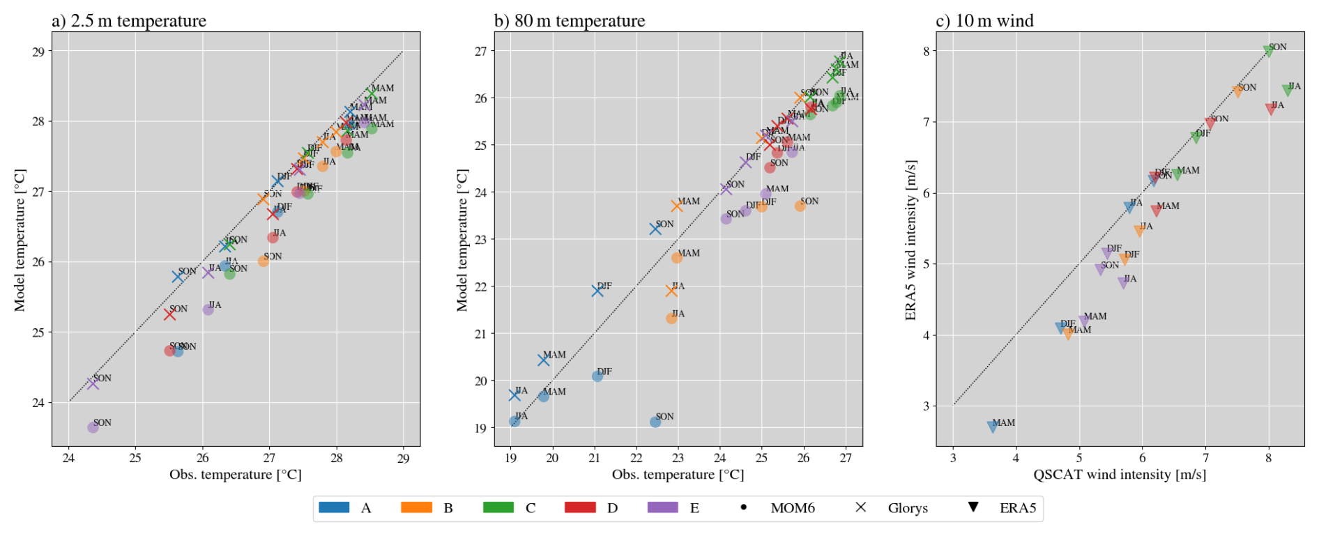
Figure A1 As in Fig. 5: Seasonal 2.5 and 80 m temperatures and 10 m winds, compared against observations. The graphs display the temperature at 2.5 m (a) and 80 m (b) for the model and reanalysis compared to PIRATE buoy observations. In (c), the atmospheric forcing for the model, 10 m wind from ERA5, compared to QSCAT satellite observation (Hoffman and Leidner, 2005). Colors distinguish the buoy sites from A to E. The model data is obtained with the z^∗ vertical coordinate and marked with circles, extending from 1997 to 2017. The reanalysis from Glorys takes crosses and ERA5 triangles. The seasons are named as DJF, MAM, JJA, and SON.