the Creative Commons Attribution 4.0 License.
the Creative Commons Attribution 4.0 License.
 | 09 Mar 2026
Implementation of a dry surface layer soil resistance in two contrasting semi-arid sites with SURFEX-ISBA V9.0
Jannis Groh
Guylaine Canut
Aaron Boone
Estimating latent heat fluxes in semi-arid environments remains challenging due to the strong spatial heterogeneity of soils and plants, land management practices, and limited observational data. In particular, accurately predicting the partition of evapotranspiration into evaporation and transpiration from observations remains very challenging. Land surface models (LSMs) can be used as a tool in this regard, when their validation is possible, but recent studies have indicated that LSMs generally overestimate soil evaporation.
This study evaluates the performance of the land surface model ISBA within the SURFEX platform using data from two contrasting sites during the Land surface Interactions with the Atmosphere over the Iberian Semi-arid Environment (LIAISE) field experiment: an alfalfa field subjected to flood irrigation, and a natural grassland which is nearly senescent during the study period. It was found that the ISBA model tended to overestimate the evapotranspiration. Therefore, a dry surface layer (DSL) resistance was implemented in the ISBA model to improve the simulation of evaporation, which has proved successful in other models. The implementation of a DSL resistance led to an improvement in the simulated latent heat flux by reducing bare soil evaporation compared to simulations without a soil resistance. This approach reduced the daily RMSE of the latent heat flux by 29 % and 32 % at the alfalfa and natural grass sites respectively, while marginally increasing the correlation at both sites. Sensible heat flux and net radiation have improved on the order of 10 W m−2, whereas the ground heat flux has deteriorated within the same order. The resulting DSL simulations reduced the overall global error compared to a simulation without a DSL resistance. A sensitivity test of the parameters that drive a DSL resistance in ISBA further improved the simulations, reducing excessive diminution of LE after rain events. The new DSL parameterization helps overcome current problems of ET modeling by reducing bare soil evaporation within LSMs.
- Article
(8474 KB) - Full-text XML
- BibTeX
- EndNote


Semi-arid environments are characterized by water deficits during part of the year. In these areas, water resource management is essential for food production and water use for the local population, as water scarcity is common. In particular, the estimation of water loss by evapotranspiration (ET) is a challenge in these areas due to several factors, such as the significant heterogeneity of land surface characteristics, low values of fluxes at the limits of observational capabilities (Mauder et al., 2020), anthropic changes in land use such as the harvesting of crops and in land management such as irrigation, and complex underrepresented processes in the unsaturated zone of the soil (e.g. secondary drying fronts, pore scale influence such as in Or et al., 2013). As a result, such processes are still being studied and incorporated to the models. Global estimates of ET reveal seasonal differences depending on the product (Jiménez et al., 2011) and the method (Coenders-Gerrits et al., 2014; Schlesinger and Jasechko, 2014). The transpiration ratio, the proportion of water vapor released through transpiration relative to total ET, is critical in assessing the potential improvement of water use through the regulation of transpiration (Yoo et al., 2009). Estimates of the ratio range from transpiration-dominated (Miralles et al., 2011) to evaporation-dominated (Alton et al., 2009) ecosystems when estimated from satellite and model-derived ET. The observed range of transpiration ratios, from 38 % to 77 %, can largely be attributed to differences in leaf area index (LAI) estimates across the reviewed studies (Wang et al., 2014). Since LSMs tend to have a low transpiration ratio (Chang et al., 2018) and tend to overestimate the evaporative fraction and the bare soil evaporation after rain events (Lohou et al., 2014), a better representation of soil resistances can serve to improve the soil evaporation in the models, leading to better partitioning of ET and a reduction in near surface temperature biases in atmospheric models (Dong et al., 2020).
LSMs estimate ET and its partitioning with varying complexity (Noilhan and Planton, 1989; Sellers et al., 1996; Coudert et al., 2006; Napoly et al., 2017). ET estimates can be made without distinguishing between sources, as in the Priestley-Taylor or Penman-Monteith methods, or by partitioning ET into bare soil evaporation, transpiration and evaporation from the interception of residual water on the leaves using similarity theory. Transpiration is modeled using a resistance analogue together with the humidity gradient. The resistance represents the canopy biophysical processes. One of the configurations includes the assimilation of carbon, which allows the specification of species-dependent plant parameters.
Bare soil evaporation in the unsaturated zone is characterized by the simultaneous presence of water in both liquid and vapor phases within the soil. Explicit treatment of soil water vapor requires full coupling between the transfer of heat and the transport of water (Philip and De Vries, 1957; Milly, 1984), which is very sensitive to soil hydraulic properties (Chanzy et al., 2008; Merlin et al., 2016). They can modify the behavior of capillary continuity and exchange processes from pores through air to the atmosphere, determining transport processes across soil drying stages (Or et al., 2013). Up to four stages of drying soil can be identified (Zhang et al., 2015): (1) stage of ponding, (2) a period of air intrusion into the soil, (3) a rapid drying until no liquid remains and, (4) a residual layer drying as the vaporization plane descends and a dry surface layer (DSL) forms (Balugani et al., 2018). A more common approach is to separate soil evaporation in two stages. Stage 1 depends mostly on the atmospheric energy demand and drives a constant rate of evaporation. Stage 2 evaporation is controlled by the soil characteristics. The rate of evaporation depends on the type of soil and its soil hydraulic properties (Schneider et al., 2021). The implicit treatment of bare soil evaporation can be modeled by a soil resistance thereby simplifying the coupling that depends on radiation, liquid water gradients and temperature gradients to a dependence on water content, and in some cases, also on the temperature. Such empirically-based soil resistances have been used for years in various land surface models (Sellers et al., 1992b; Best et al., 2011; Harris et al., 2017; Raoult et al., 2018), as simulated latent heat fluxes (especially from the soil) were found to be overestimated in their respective models. The tuned values of these resistances can have a large impact on the water balance components in addition to the evaporation, such as for the runoff (Cuntz et al., 2016).
More recently, models have applied more data-driven approaches (Merlin et al., 2016; Lehmann et al., 2018; Raoult et al., 2021) to constrain case-dependent results and physically based resistances (Sakaguchi and Zeng, 2009; Zhang et al., 2015; Swenson and Lawrence, 2014) as knowledge of soil physics advances. These resistances differ in the value of the volumetric water content (VWC) at which they become active, whether its form is exponential or linear, and in terms of the magnitude of the resistance. Two resistances are of particular interest, the first by Sellers et al. (1992b) due to its longstanding wide use, and the second by Swenson and Lawrence (2014) which is based upon a more physically meaningful resistance with larger values (more details are provided in Sect. 2.2.1). The aforementioned study used the FLUXNET dataset (Jung et al., 2009) and a model tree ensemble approach to analyze behavior on a global scale. By implementing the DSL in the Interactions Soil-Biosphere-Atmosphere (ISBA) model (see Sect. 2), we investigate whether it can improve its estimation of bare soil evaporation and consequently ET.
Both the Sellers et al. (1992b) and the Swenson and Lawrence (2014) parametrizations are tested in detail for two sites that were operated during the Land surface interactions with the atmosphere over the Iberian Semi-arid environment (LIAISE) campaign, described in Sect. 3.1. They represent the extremes found in the semi-arid environment in terms of Bowen ratio: the first site is a flood irrigated alfalfa field where ET dominates, and the second is an almost senescent rainfed natural grass site where sensible heat flux dominates. Together these two sites provide a good test case for studying the limits of the model and for evaluating the default and new parametrizations with a DSL.
ISBA includes a Multi-Energy Budget (MEB) model option described in Boone et al. (2017) which uses a classical Big-Leaf type approach for modeling the surface energy budget (SEB). MEB separates latent heat flux (LE) as the contribution of soil evaporation, transpiration, interception of evaporation and sublimation when snow is present. It allows separate consideration of vegetation-driven processes, such as the impact of stomatal conductance and light assimilation on transpiration, and of soil processes, such as soil evaporation and the impacts of a litter layer. MEB can also represent vertical heterogeneity of the soil hydraulic and thermal properties across the soil profile. ISBA-MEB within SURFEX (Surface Externalisée: Externalized Surface) version V9 is used in this article together with the multilayer diffusive soil scheme option (Decharme et al., 2011). To date, the local scale evaluation of ISBA-MEB has been carried out with trees (Napoly et al., 2017), corn (Dare-Idowu et al., 2021) and in a semi-arid environment in a vineyard (Aouade et al., 2020).
2.1 Components of the latent heat flux
The LE can be found by the evaporative contribution of the vegetation and the soil:
where Lv is the latent heat of evaporation and Eg is the part of the flux originated from soil evaporation (see Sect. 2.2). Ev is given by the sum of the plant transpiration Etr and the evaporation from the canopy liquid water interception store Er, when no snow is present. The description for the vegetation description of the model can be found in Appendix A with a glossary in Appendix D. For completion, the G flux is also described in Appendix C1.
2.2 Bare soil model formulation
The SURFEX V9 MEB bare soil evaporation with soil resistance consists in a mixed form soil resistance such as in Niu et al. (2011), Xue et al. (1996) and Sellers et al. (1996). A mixed formulation consists in adding a soil resistance (beta type formulation) to the aerodynamic resistance while also using a soil humidity factor applied to the saturated specific humidity in the numerator (alpha type formulation). This added mixed formulation is incorporated in the ground evaporation expression as:
Rag is the air resistance (s m−1), Rsoil is the soil resistance, qsat g is the saturated specific humidity of the air calculated with temperature of the ground at its first layer and hu is the soil humidity coefficient which has the form:
and when and qsat g>qc then either there's no soil evaporation because the low level humidity is dry (Eg=0) or and qsat g≤qc which implies condensation (Noilhan and Mahfouf, 1996). The default version of ISBA only included the humidity factor, hu (and thus was uniquely an alpha formulation).
2.2.1 Soil resistances
The overestimation of ET in land surface models is a lingering issue (Lohou et al., 2014). In particular, it has been shown that bare soil evaporation is generally overestimated in LSMs (Chang et al., 2018), leading to overestimation of global ET (Wang et al., 2021). In addition, the partitioning of ET into transpiration and soil evaporation is the main source of inter-model differences among different models (Feng et al., 2023). Several forms of soil resistance have been proposed over the years (Barton, 1979; De Silans et al., 1989; Sellers et al., 1992b; Van de Griend and Owe, 1994; Xue et al., 1996; Camillo and Gurney, 1986; Mohamed et al., 1997; Ding et al., 2015; Ivanov et al., 2008; Merlin et al., 2016; Swenson and Lawrence, 2014; Lehmann et al., 2018; Raoult et al., 2021), some of which have been tested within ISBA (Béziat et al., 2013). The early citations were based on identifiable changes in the soil, while satellite information has been added in more recent years.
De Silans et al. (1989) reported that the influence of soil resistance on evaporation was significant and goes along with a change in soil color together with a change in albedo measurements. Van de Griend and Owe (1994) observed the superficial DSL color change to a soil depth of 2.5 cm, together with a lower volumetric water content compared to the underlying layer and an increased estimation of the soil resistance value. The soil drying process of the DSL has been explored in laboratory conditions (Or et al., 2013; Zhang et al., 2015; Wang, 2015; Merz et al., 2016; Balugani et al., 2021). The results of these studies have led to a better understanding of the DSL formation process, and its impact on ET. Other processes, such as corner and film flow, are being explored in other communities and allow the identification of soil hydraulic properties with models such as HYDRUS in medium to dry conditions (Iden et al., 2021), but this level of sophistication falls outside the scope of this article.
The formulations cited here all produce lower resistance values than Sellers et al. (1992a) except for the DSL resistance as implemented by Swenson and Lawrence (2014). A comparison of resistance values for several standard soil resistance formulations over a range of soil water contents is shown in Fig. 6 of Swenson and Lawrence (2014), which shows that the DSL approach has the largest values. The DSL resistance was tested successfully globally in Swenson and Lawrence (2014). In the current study, we investigate this method in detail using the LIAISE data.
2.2.2 Sellers, 92
A widely used expression for soil resistance among LSMs, such as the community Noah-MP (He et al., 2023), PX LSM WRF/CMAQ (Ran et al., 2016), ISBA-MEB (Boone et al., 2017), ORCHIDEE (MacBean et al., 2020) originated from Sellers et al. (1992b, 1996) and is formulated as:
where A=8.206 and B=4.255 (Sellers et al., 1992b). These values were computed using field measurements taken during the FIFE 89 campaign in Kansas (Sellers et al., 1992a) by inverting the SiB model (Sellers et al., 1992b) and finding the best fit for several sites in the area.
2.2.3 Dry soil layer resistance
A DSL resistance is tested in SURFEX as an alternative for a soil resistance to Sellers 92. It models sites where compaction and very intense heat cause all liquid water to be lost in the first few centimeters. This results in the formation of a DSL that makes evaporation difficult: this impediment to evaporation is due to the transport of water being done only by vapor water diffusion. This process is modeled in a pragmatic manner by using a surface layer resistance. According to Swenson and Lawrence (2014), a DSL can be parameterized by the equation:
where Δzdsl is the length scale of the maximum ΔDSL thickness (m) and is given a value of 0.015 m as in Swenson and Lawrence (2014), and wdsl0 is the moisture value at which the DSL becomes active. wdsl0 depends on the porosity (Φ) from wdsl0=KdslΦ where Kdsl=0.8 is the value found by Swenson and Lawrence (2014) which improves their ET estimation in semi-arid conditions. The porosity is defined as the saturated volumetric water content (wsat,1) of the first layer, as this corresponds to the pore space available for water. wg,1 corresponds to the moisture value at the top soil layer of the model, while wair is the “air dry” soil moisture defined as
where the air dry matric potential is m, the saturated matric potential is represented by Ψsat and the slope of the soil water retention curve is b. The soil resistance is expressed as
where τv is the tortuosity of the vapor flow paths through the soil matrix and is the molecular diffusivity of water vapor flow in air (m2 s−1). The expression of differs slightly from that used in Swenson and Lawrence (2014) through the dependence on pressure, p, and the exponent of temperature:
where p0 is a standard reference pressure (1000 hPa), Tg,1 being the first level of soil temperature and Tf is the freezing temperature of water. The tortuosity is then given by:
where and represents the air-filled pore space.
3.1 The LIAISE campaign
The LIAISE campaign (Boone et al., 2025) was designed to improve the understanding of the impact of anthropization on the water cycle in semi-arid environments, with a particular focus on identifying the limitations of LSMs under these conditions. The field experiment took place in the north-eastern region of the Iberian Peninsula from April 2021 to the end of September 2021 (the Long Observational Period, LOP). Surface energy budget stations were installed over alfalfa (Canut, 2022a; Mangan et al., 2022), maize (Martínez-Villagrasa et al., 2022), irrigated grass (Miró, 2021), vineyard, apple orchard, almond orchard (Canut, 2022b) and natural rainfed grass (Price, 2023). They consisted in eddy-covariance systems equipped with a gas analyser to measure the turbulent fluxes and buried sensors including buried temperature sensors and flux plates, allowing the measurement of the ground flux directly and correction of its measurement to the surface (see Table E1) with the calorimetric method (De Silans et al., 1997). An intensive Special Observation Period (SOP) took place during 15–29 July (Boone et al., 2025), with in-situ measurements of soil and vegetation properties and of the atmospheric boundary layer (ABL) up to the entrainment zone through a multi-institutional collaboration (Brooke et al., 2023). The region is characterized by an irrigated area with fruit trees, maize and alfalfa, and a rainfed area with wheat, olives, almonds and natural grassland. The two areas are separated by the Canal d'Urgell. This configuration creates a profound contrast in the SEB components between the areas. The two main sites of the campaign, La Cendrosa and Els Plans, included a 50 m tower, SEB station and meteorological measurements, radio soundings, LAI and vegetation height observations (Boone et al., 2025). Two surface stations were installed at la Cendrosa, the longer series was taken (Canut, 2022a). Measurements of temperature, humidity and wind at different levels depending on sensor availability and high frequency measurements were available 3, 10, 25 and 50 m for the two sites (see Boone et al., 2025 and Brooke et al., 2023 for more details).
3.2 Irrigated alfalfa site: La Cendrosa
The La Cendrosa site is located within an alfalfa field that was irrigated by gravity flooding approximately every ten days during the growing season and periodically cut for harvest. A cycle of cutting and growing during the month of July 2021, characterized by in-situ values of LAI and vegetation height, is prescribed as input (Fig. 1) for ISBA. The period starts with fully grown vegetation, but after a few days, the vegetation is cut. Growth starts rapidly after the next irrigation period and the vegetation height increases from about 10 cm to its maximum height of approximately 70 cm in 17 d. The LAI increases accordingly (from 0.3 to 3) over the same period. This rapid vegetation evolution has an impact on the observed fluxes (Fig. 2). Initially, the net radiation (Rn) starts at values near 680 W m−2 and decreases a few days after mowing. However, the change is not immediately apparent in the measurements as it takes several days for the harvested alfalfa to be removed from the soil as it is left to dry in the field. After the initial growth period, when LAI is sufficient to cover most of the soil, the Rn returns to values close to 600 W m−2. These observed values are not as high as before harvest because the water content is lower than after irrigation and this results in a higher albedo (see Sect. 5.3). LE is the dominant flux at this site, and the ground heat flux (G) and the sensible heat flux (H) represent a small part of the energy balance, except for the period after cutting and at the beginning of the growing period. The energy balance residue (Res) can be 100 W m−2 and negative during the day. It is defined as the residual available energy remaining after the Rn has been redistributed in the atmospheric and ground heat fluxes. The highest values of the residual are observed during periods of high vegetation. When vegetation is low, the value of the residue remains low or negative.
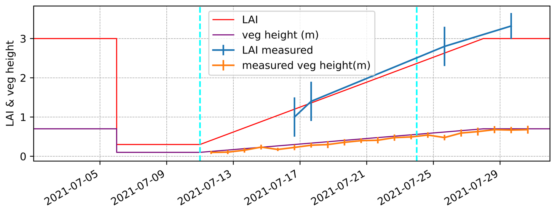
Figure 1Cycle of cutting and growth of alfalfa at La Cendrosa site. Imposed Leaf Area Index (LAI) in red, measured LAI in blue, vegetation height in purple and measured vegetation height in orange.
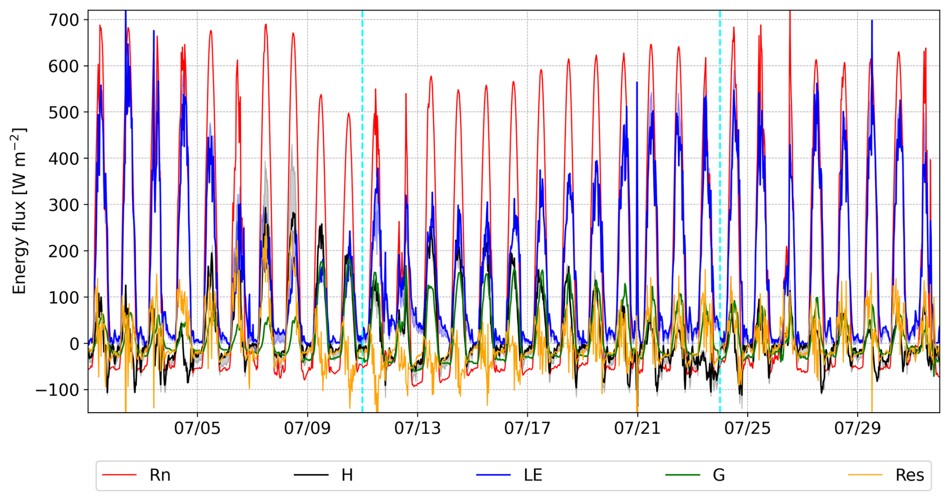
Figure 2Observed terms of the Surface energy budget of La Cendrosa for the month of July 2021. In particular, Rn in red, H in black, LE in blue, G in green and the Res in orange. The gray and blue shading correspond to the error in the H and LE due to the Res, which is accounted for by the Bowen ratio. Cyan dashed lines indicate irrigation events and the gray line indicates the cutting of the alfalfa.
3.3 Dry rainfed natural grass site: Els Plans
The Els Plans site is a rainfed, relatively dry area with natural grass that was drying during the LOP. The parcel is located within a special protection area for steppe birds, and it is not cultivated. The energy budget of a short dry-down period near the end of the LOP (Fig. 3) shows a lower Rn compared to La Cendrosa with two small rain contributions of 2 and 0.8 mm on the eve of 2 September. The Rn difference is due to the contribution of the net long wavelength radiation being lower and the time difference between the two periods which can account up to 100 W m−2. The small amount of available water in the soil makes the H the dominant term to compensate the Rn. The G can reach values twice as high as the LE, except after rain events, when the evaporation from the bare ground peaks. The energy budget residual at this site tends to be greater in the early morning, and it is reduced after the entry of the Marinada, a local sea breeze wind (Jiménez et al., 2023). This behavior is also observed in La Cendrosa when the vegetation is low. As a colder wind (Lunel et al., 2024), the Marinada advects moisture and cool air, and contributes negatively to the energy budget, bringing the residue closer to zero.
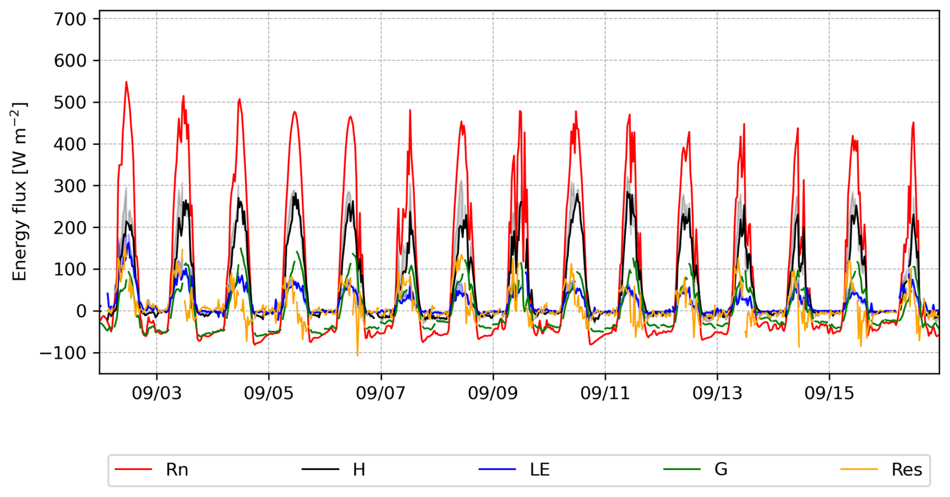
Figure 3Observed terms of the Surface energy budget of Els Plans for a dry down period. In particular, Rn in red, H in black, LE in blue, G in green and the Res in orange. The gray and blue shading correspond to the error in the H and LE due to the Res, which is accounted for by the Bowen ratio.
4.1 Forcing data
The La Cendrosa and Els Plans simulation are performed offline (i.e. driven by observations as input). They comprise the periods from 1 July at 00:00 UTC to 1 August at 00:00 UTC and from 17 June at 10:00 UTC to 29 September at 09:00 UTC respectively. The associated atmospheric variables include the incident short and longwave radiation fluxes, wind speed, temperature, specific humidity, pressure, atmospheric CO2 concentration, and rainfall rate at a 30 min time step. All measurements were taken at 2 m except the wind which was measured at 10 m and precipitation that was measured at 1 m for both stations. The time evolving vegetation properties are usually imposed using a 10 d or monthly time step. For the current study, however, this temporal resolution is insufficient (more detail in Sect. 4.2.1). For Els Plans, several incidents in the availability of electric current after rain events resulted in gaps in the input variables. Short-wave radiation was gap-filled using a theoretical, solar zenith-dependent method. Long-wave radiation gaps were filled using the correction proposed by Brutsaert (1975). Wind speed gaps were filled with additional wind measurements at 3 m from the same site, corrected by adjusting the wind speed to that which was already measured at 10 m above the surface assuming a logarithmic profile at neutral conditions. Pressure was gap-filled with a fixed average value during the same period. Since the albedo of the soil changes with variations in water content, values are taken into account every 10 d. For La Cendrosa, irrigation was treated as rainfall by adding 30 mm of water between 00:00 and 02:00 UTC. This approach introduces error for about four hours as it simulates an increase in evaporation of intercepted water over the leaves, the latent heat increases up to 130 W m−2 when vegetation is low and close to 70 W m−2 when it is high. The LAI and vegetation height cycle (shown in Fig. 1) cause the global albedo to change dynamically.
4.2 Parameter selection
Table 1 shows the parameter values for the different model configurations. The prescribed dynamic roughness length (z0) for both stations falls within the lower limits of the tabulated values in the literature (Oke, 2002). For La Cendrosa, a single value is chosen as it gives reasonable estimates of the momentum for the whole period. The roughness length and the displacement height depend not only on the height of the vegetation but also on the density of the vegetation (Foken and Napo, 2008). These dependencies are still being parametrized (see the background in Jasinski et al., 2005), and are not currently modeled in ISBA. Therefore, a compensatory effect between changes in these two processes may be at play. For Els Plans, the roughness generating elements remain constant throughout the study period. The thermal roughness length (z0 h) is smaller at La Cendrosa, which shows less steep temperature profiles near the surface in the presence of dense vegetation. The emissivity values are within the indicated error margin of the tabulated values and have been set to 0.97 for both sites (Snyder et al., 1998; Simó et al., 2019). However, it should be noted that the sensitivity to this parameter has been found to be low for this parameter for the ranges encountered at the two sites studied herein. For the type of vegetation of the alfalfa field, the C3 crop type is selected and C3 natural grass is used for Els Plans (Table 1).
Table 1SURFEX parameters characterizing the simulations of the Els Plans and La Cendrosa sites. In order, the dynamic roughness length (z0), heat roughness length (z0 h), the number of soil layers, the SURFEX patch identifier (7 corresponds to C3 crops and 10 corresponds to natural grass), the range of leaf area index (LAI) and the height of the vegetation (Hveg) during the study period.
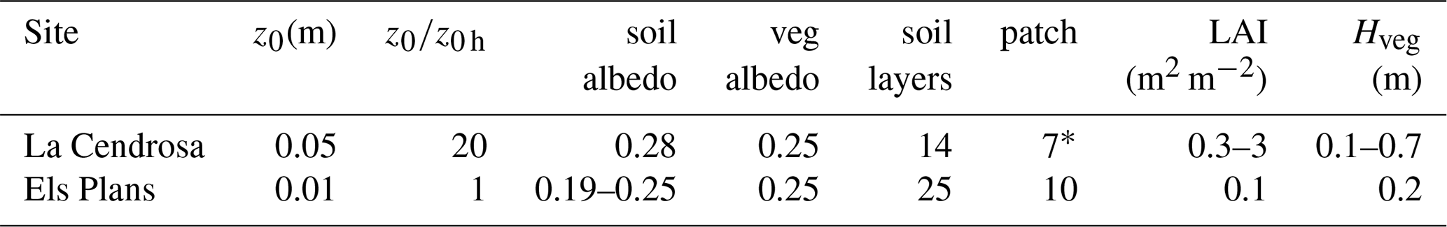
* The strategy has been changed to drought-tolerant.
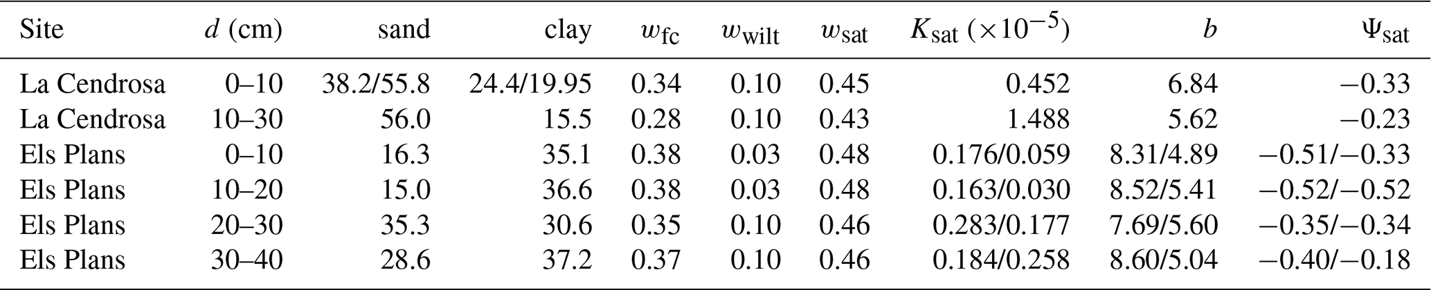
Table 2SURFEX parameters characterizing the soil properties of the Els Plans and La Cendrosa sites. The columns, in order, represent the depth (d), the sand and clay content, the water field capacity (wfc), the wilting point (wwilt) water content, the saturated water content (wsat), the saturated hydraulic conductivity (Ksat), the b parameter of the CH78 pedotranfer function and the soil water potential at saturation, Ψsat.
4.2.1 Vegetation characterization of alfalfa
A realistic simulation of transpiration is the key to providing a good estimate of the LE, especially for the alfalfa. The changes of LAI for La Cendrosa (Fig. 1) are imposed every time step compared to the original code since the alfalfa growth is relatively rapid (see Sect. 3.2). The height of the vegetation is modeled using a linear dependence on LAI based on the observations. Additionally, the AST option within SURFEX is used for both simulations. With this option, the A-gs scheme is used to model photosynthesis parameterizing its processes in contrast with other options that model transpiration directly without considering the biological processes. The vegetation can have either drought tolerant, Eq. (A9), or drought avoidant strategies, Eq. (A7), (Calvet et al., 2004). Direct observations of stomatal conductance (gs), CO2 assimilation and photosynthetically active radiation (PAR) were made at la Cendrosa. After testing multiple parameter configurations, it was found that increasing the quantum efficiency, ϵ0, and the maximum assimilation (Am,max(25)) gave results that reproduce results obtained with a higher cuticular conductance (see Appendix B1 for more details). The following changes to the vegetation parameters are imposed:
-
Mesophyll conductance. Although alfalfa is a C3 crop, its drought strategy is tolerant as in C4 crops. Such plants species are known as C4-like species (Way et al., 2014). In consequence, the stress type has been changed to drought tolerant for the simulation. The values have been changed to 0.005 m s−1 (see Table B1).
-
Quantum efficiency. The ϵ0 value of 0.0265 mg CO2 J−1 found by González-Armas et al. (2024) increases the LE to values closer to the observed values and is therefore used in this study.
-
Maximum assimilation: González-Armas et al. (2024) found values (3.02 mg) at La Cendrosa that were considerably higher than those given in the literature and the standard value in SURFEX. Increasing this value in this simulation improves the transpiration estimates for days that show a dip in LE during the day reducing its intensity, therefore the value in González-Armas et al. (2024) is kept, but the default values are adequate for most of the simulated days.
An extended version of this section is in Appendix B1 with detailed justification over the parameter changes and its bibliographical context.
4.2.2 Vegetation characterization of drying grass
For Els Plans, the choice of LAI is complex. Measurements of LAI at the site have a median value of 0.34 m2 m−2 and a minimum value of 0.12 m2 m−2 (Brooke, 2023). However, these measurements take into account the shaded area by the vegetation and do not necessarily represent active vegetation. In contrast, in ISBA LAI is taken as green LAI and therefore represents fully active vegetation (Brut et al., 2009). This does not correspond well with the measurements in Els Plans, where the vegetation is dying but still provides shade and intercepts moisture. Furthermore, this shade is provided by the blades of the natural grass rather than the leaves. The value of LAI =0.1 m2 m−2 is used as a compromise to take into account the shaded ground and part of the dry vegetation that does not contribute to evaporation, thus limiting transpiration.
A complementary parameter necessary to characterize the vegetation is vegetation height (Hveg), which tests show is not a highly sensitive parameter for either site and is set to 0.2 m by rounding the observed value of 0.16 m for Els Plans. In healthy active low vegetation such as crops, LAI may not be directly related to its height or it may depend on the crop so they are set independently (Yuan et al., 2013).
4.2.3 Soil characterization
Table 2 lists the measured sand and clay content values together with the soil hydraulic parameters obtained from the soil texture data and the pedotransfer function from Clapp and Hornberger (1978), referred to herein as CH78. For La Cendrosa, two surface measurements of the soil characteristics were carried out by different teams. The first measurement was taken near the SEB station at two levels; the second measurement was taken about 20 m away within the same field. The second measurement had proportions of sand and clay close to those at a depth of 10–30 cm of the first measurement. Since the field is irrigated by flooding, some washing of the soil can take place, which can be the source of these near-surface discrepancies in texture between the samples taken by the different teams. The two-level measurements are used for La Cendrosa for all parameters except the wilting point of the model. This parameter is reduced to include the minimum water content within the root zone, as seen in the observations. At the Els Plans site, a more extensive soil sampling was performed and incorporated, so that the matric potential at saturation Ψsat, the slope of the retention curve b and the saturated hydraulic conductivity Ksat values were fitted from soil core samples using the HYPROP method (Shokrana and Ghane, 2020) and Ksat values were measured in the laboratory. The Ψsat value differed from that given by CH78 at the surface and bottom of the soil profile and the b parameter is at the lower end of its range. Using these vertically-varying observed values reduced the overall error of the simulation compared to using a constant values for the vertical profile of the soil and compared to the default values taken from the global database. This matches the results of Sobaga et al. (2023) who identified that the default b parameter produced a lack of drainage in SURFEX V8.1. Ksat is taken as the observed value instead of the fitted one, as it also leads to an improvement in the LE and H estimation. We note that it differs by an order of magnitude at the surface. Soil layers deeper than those observed were assumed to have the same soil properties as that in the lowest observed layer. The discretization of the soil layers has been chosen to match the layers to the depth of the observations, while maintaining the highest vertical resolution near soil column's surface.
4.2.4 DSL parameters
The DSL configuration for the main comparison is the one of Swenson and Lawrence (2014) but its parameters may not be the most suitable for ISBA. A sensitivity analysis, consisting in the variation of two parameters for the DSL resistance is later presented. This type of analysis is necessary to characterize and diagnose changes in output variables. The response to the change can be identified, whether it is linear, nonlinear or negligible. As the number of parameters increases, output behaviors become intertwined and cannot necessarily be easily predicted. The sensitivity analysis identifies whether a parameter is relevant for a certain variable. We generate multiple simulations with two varying parameters and use the root mean square error (RMSE) of the simulations to suggest the more appropriate values for estimating of the turbulent fluxes with ISBA for the DSL option.
This section presents an analysis of the simulations carried out for La Cendrosa and Els Plans using the default and new soil resistance parameterizations. The different simulations are identified by the names NON, S92 and DSL to indicate no soil resistance, the use of Sellers 92 resistance and a DSL resistance, respectively.
According to Foken and Napo (2008), a bulk indication of instrumental errors indicates that Rn can have errors of around 10 %, errors in H and LE can reach 20 %, together with a 50 % error for the G, not accounting for the energy storage error. Note that budget closure is not necessarily a measure of the quality of the fluxes (Aubinet et al., 2000). The lack of closure in observations is expressed as residual energy. It includes part of the instrumental error, but also owing to horizontal advection due to heterogeneity (not modeled), heat storage due to vegetation and its exchanges (modeled in ISBA-MEB but considered small compared to soil storage under normal circumstances), and unmeasured phase water changes in the soil (not modeled) (Cuxart et al., 2015).
As mentioned in Sect. 3.3, the local sea breeze reduces the residue, so some advection contribution to the residue is expected. Consequently, the main analysis focuses on comparing of fluxes with the simulation without imposing closure on the observed fluxes but the statistical comparison is also shown with the closure imposed by the Bowen ratio method (Barr et al., 1994).
5.1 The simulated energy budget
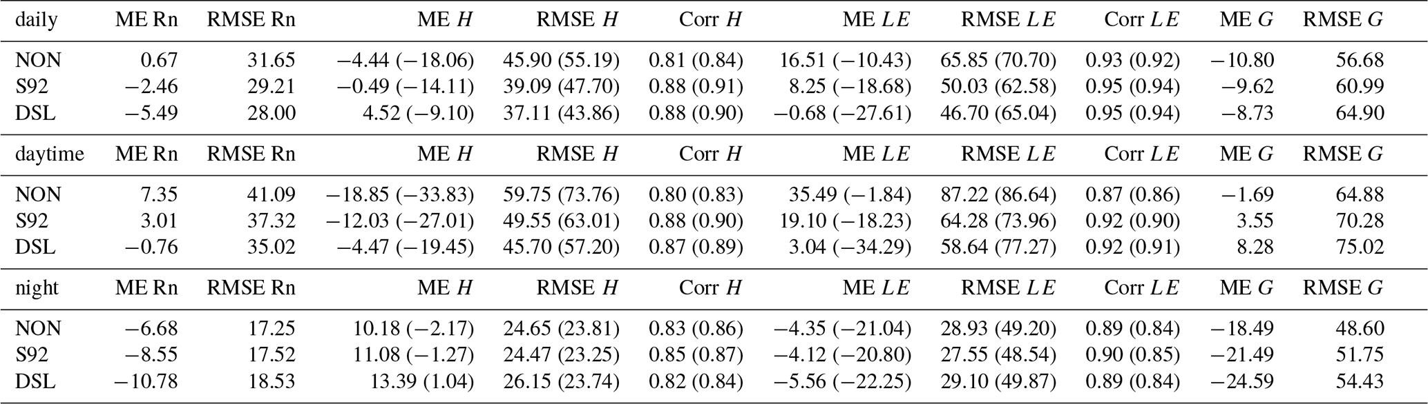
Table 3 shows the statistical comparison of the energy budget for La Cendrosa, divided into three time periods; daily, daytime and night. The distinction between daytime and night is made from 08:00 a.m. to 08:00 p.m. UTC, leaving out the more complex changes of the transitions in the night period since the main changes caused by the use of a resistance occur during the day. The following analysis focuses on the daytime, so that behaviors resulting from certain periods, such as low and high vegetation or flooding events, can be identified. A comparison of the simulated and observed Rn is shown in Fig. 4 a and e. Despite the mean error (ME) indicating a bias close to zero, the NON simulation is positively biased overall. This behavior is improved through the use of the DSL scheme. In particular, two days show a different trend that modifies the statistics (Table 3). This behavior corresponds to the period between the cutting and the removal of the alfalfa, which took place a few days later. The effect that the resistances have on the Rn is mainly due to the difference in the longwave energy budget and surface temperature, since the soil emits less heat in the NON simulation, and the albedo input does not change between simulations. The LE flux shown in Fig. 4b and f is centered on the one-to-one line. A subset deviates from the line and corresponds to the period of low vegetation with relatively low LAI after the irrigation period. The improvement in LE is shown by a reduction in ME, RMSE and an increase in correlation (see Table 3). For the H, the larger errors are corrected with the use of a resistance to compensate for the change in LE. The statistics improvement is also present for H, with the underestimation being reduced, and the RMSE reducing to 37 W m−2 for La Cendrosa and 45 W m−2 for Els Plans. These values are within the values of the standard deviation observed for the residue for La Cendrosa (56 W m−2) and Els Plans (50 W m−2). On the other hand, the simulated soil stores and releases energy faster than observed. This daily cycle is characterized by a hysteresis effect that overestimates during the day and underestimates at night thus worsening the results for G. The resistance also impacts the nighttime statistics with a reduction of the Rn that results in a lower available energy at night, and an small increase of ME and RMSE for LE and H of the order of 1 W m−2.
Table 3Mean Error (ME) and Root Mean Square Error (RMSE) in W m−2 for the net radiation (Rn), the sensible heat flux (H), the latent heat flux (LE), and the ground heat flux (G) for La Cendrosa site. The correlation (Corr) between simulation and observation has been included for H and LE. The values taking into account the residual using the Bowen ratio method are indicated in brackets.
At the Els Plans site, the Rn is well represented by the imposed albedo (Fig. 5). The error of Rn (Table 4) remains well below the 10 % error of the measurement. The use of a DSL resistance increases the RMSE and ME up to 2 W m−2. For the LE, the scatter is large in all three simulations compared to its absolute value. There is a delay in the start of evaporation, as well as an underestimation, with absolute errors close to 50 %. The RMSE of LE is reduced during the daytime from 29 to 19 W m−2 using the DSL approach. The correlation is best for the S92, followed by the NON simulation, and closely by the DSL simulation as in this case the LE is too damped. The sensitivity to the parameters used is discussed in Sect. 5.4. For the H there is a small reduction in the RMSE but an increase in the ME, so the overall performance remains the same except for an improvement from 0.87 to 0.89 in the overall correlation. For the G performance, the intense heating of the soil is again simulated with hysteresis, with the transfer of energy being quicker in the model than that observed (Fig. 5d and h), which corresponds to a daily RMSE of 70 W m−2 (Table 4). No measurements of the thermal properties of the soil have been made, and so the default properties assigned to the observed soil texture have been taken. A sensitivity test indicated that reducing the thermal conductivity of solids in the soil by 25 % could reduce this error by reducing the G flux up to 20 W m−2, while increasing the error in the H proportionally. This value is within the range of different soil types reviewed from observations by Zhang and Wang (2017). Overall, due to the higher error in the measurements of G, estimated at 50 %, this bias in the simulation is considered tolerable. The change of Rn and H at night due to the resistances is the same as for La Cendrosa, but in this case, LE has a small improvement of the correlation of approximately 0.02, with a nearly negligible change in the overall average LE value.
Table 4Mean Error (ME) and Root Mean Square Error (RMSE) in W m−2 for the net radiation (Rn), the sensible heat flux (H), the latent heat flux (LE), and the ground heat flux (G) for Els Plans site. The correlation (Corr) between simulation and observation has been included for H and LE. The values taking into account the residual using the Bowen ratio method are indicated in brackets.
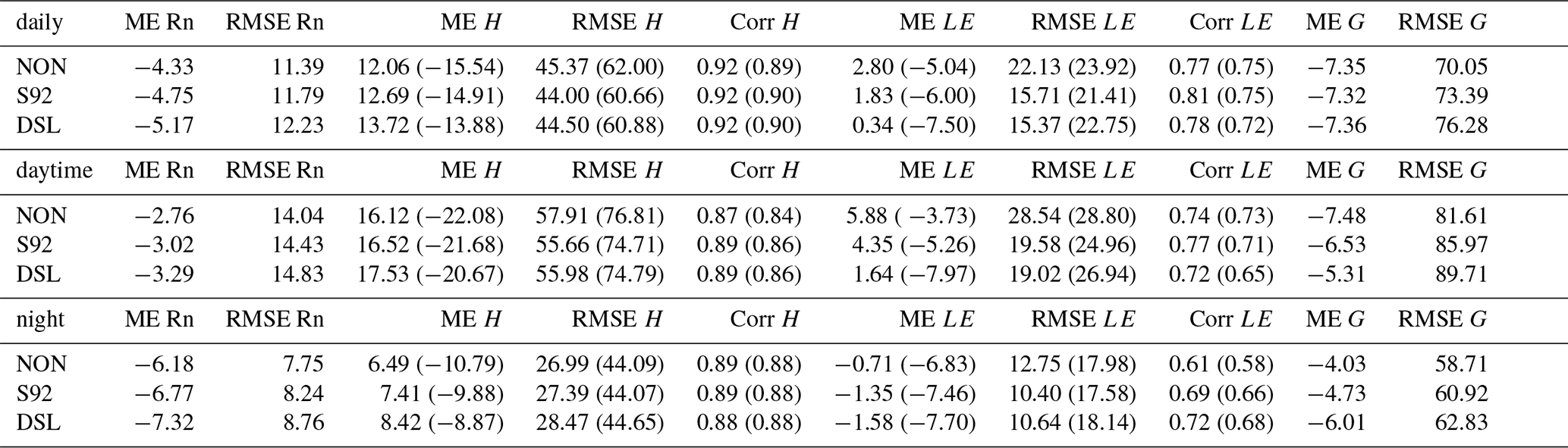
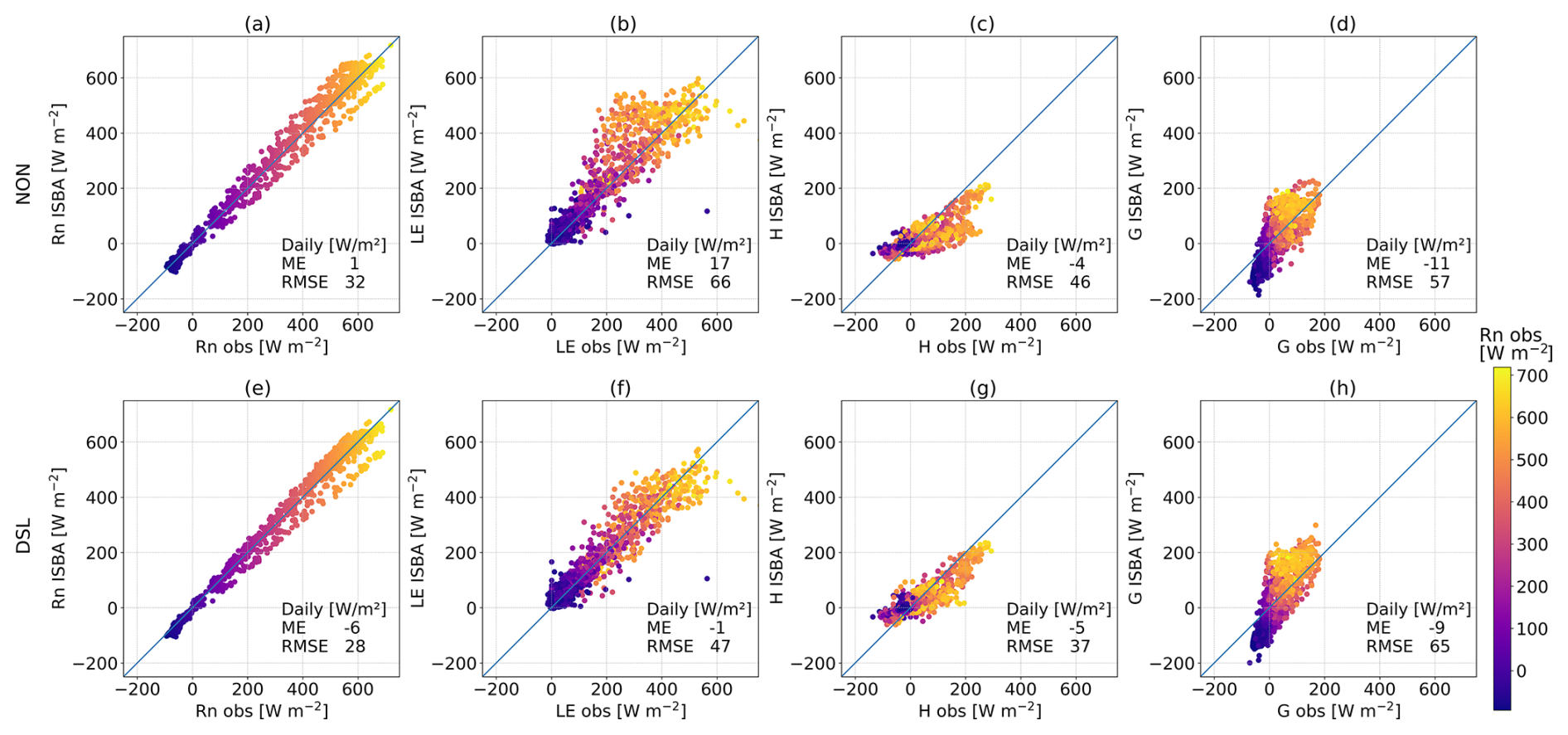
Figure 4Scatterplots of the simulated terms of the energy budget against the observation for La Cendrosa site for the NON simulation (NON, a–d) and the DSL simulation (DSL, e–h). From left to right, Rn (a, e), H (b, f), LE (c, g), and G (d, h). The simulation period is from 1 July at 00:00 UTC to 1 August at 00:00 UTC. Daily mean error and root mean square error are included in the figure frame.

Figure 5Scatterplots of the simulated terms of the energy budget against the observation for Els Plans site for the simulation with no resistance (NON, a–d) and simulation with the DSL approach (DSL, e–h). From left to right, Rn (a, e), H (b, f), LE (c, g), and G (d, h). The simulation period is from 17 June 10:00 UTC to 29 September at 09:00 UTC. Daily mean error and root mean square error are included in the figure frame.
5.2 The latent heat flux
The observed LE is shown in Fig. 6a for the aforementioned simulations, together with a bar plot from top to bottom with rain and irrigation. The largest change between simulations occurs after the first irrigation event [11 July]. The increase of observed LE is overestimated with the NON option, mainly due to the large contribution from soil evaporation, as in Lohou et al. (2014). In contrast, the LE in the DSL simulation decreases more rapidly and more accurately matches the observations during this period. The second irrigation event [24 July] and small rain events result in small increases in LE that decreases during the hours afterward, as the soil remains near saturation and has little impact on the available water. The difference in the maximum LE between irrigation events is due to the change in transpiration. The first event presents very low vegetation whereas the second is fully grown alfalfa.
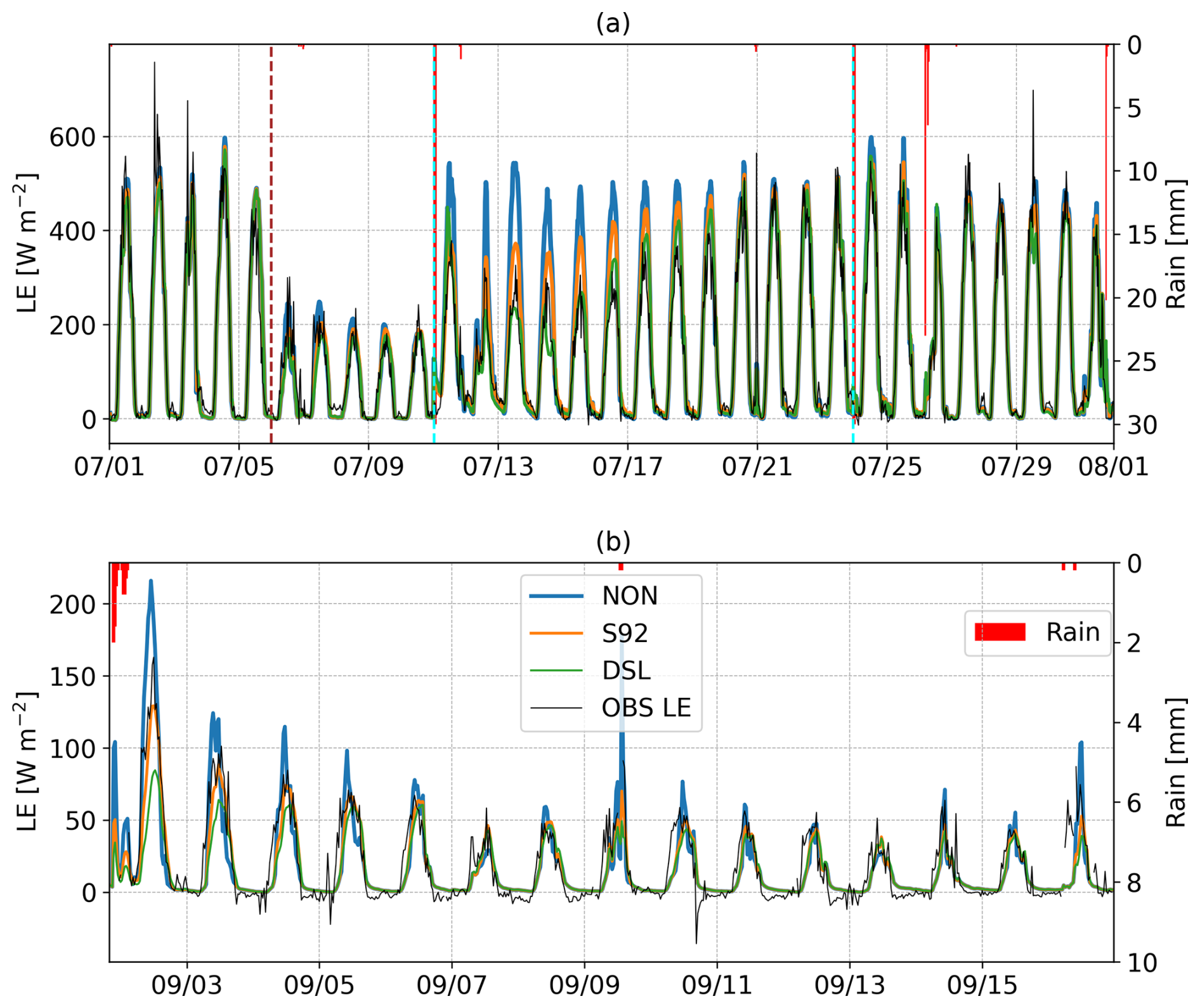
Figure 6Observed (black) and simulated latent heat flux (LE) timeseries of La Cendrosa (a) and for Els Plans sites (b) for the simulations with no resistance (NON, blue), with a Sellers 92 resistance (S92, orange) and a DSL resistance (DSL, green). Bar lines represent the rain. Vertical lines represent the vegetation cut (brown) and irrigation (cyan).
Estimates during periods of high LE are well captured by all three simulations, and it is slightly better for the NON simulation, than for the S92 and DSL simulations since the reduction of soil evaporation is not compensated by increased transpiration. The differences range from 5 % to 10 % as the soil dries. LE is also well represented during the low vegetation period for the three simulation types. The soil resistance reduces the contribution of soil evaporation to LE resulting in an improvement in the RMSE of LE (daily) of 16 W m−2 for the S92 simulation and 20 W m−2 for the DSL simulation (see Table 3).
The nocturnal LE values show good agreement with the observations, except on nights with a higher flux, during which the simulations underestimate the value (e.g. 8 July). The simulations respond well to small rain events such as the night of the 21st but with a more moderate increase. Such an increase occurs artificially in the simulation for the first irrigation event reaching 130 W m−2, as irrigation was imposed as rain, but returns to the observed values after five hours.
For the Els Plans, the interruption of the measurements after rain events mentioned in Sect. 4.1, affected the number of dry-down periods that were well captured, which limited the analysis of such events. One such period is shown where the maximum LE is better captured by S92 in Fig. 6b compared to the NON or DSL. Although this is after a rain event, the H is dominant and the magnitude of LE is small. The vegetation at this site is mostly senescent, and the water content of the first soil layers is very low. Following a rain event, soil evaporation increases and contributes significantly to ET throughout the day. Evaporation from the interception is also present in the model for about six hours and increases up to 10 W m−2. However, as the soil dries, bare soil evaporation contribution is present only in the middle hours of the day. Instead, the main contribution is attributed to the dying vegetation and shows a slower daily cycle with a slower progression in the increase in ET. The modeled transpiration values are on the order of 30 W m−2 compared to the daily maximum of LE of 50 W m−2. Nonetheless, they represent only a relatively small part of the energy budget and are of the order of the residue. For Els Plans the nocturnal observations show that negative LE values are common at night, indicating dew formation or soil water vapor adsorption, which is typical not only under such dry conditions (Paulus et al., 2024; Kohfahl et al., 2021), but also under more humid soil conditions (Groh et al., 2018a). The presented simulations have struggled to reproduce these negative values, because the soil temperatures are high and the transition to a stable regime is rare.
5.2.1 Soil resistances
Modeled soil resistances reach at their minimum values after rain or irrigation events and increase with time as the soil dries. For La Cendrosa site (Fig. 7a), the soil resistance value increases using the DSL approach and resistance values can reach up to four times that of S92. Note that the DSL resistance does not start acting until the VWC has fallen below saturation to the wdsl0 threshold, unlike the S92, which always presents some resistance.
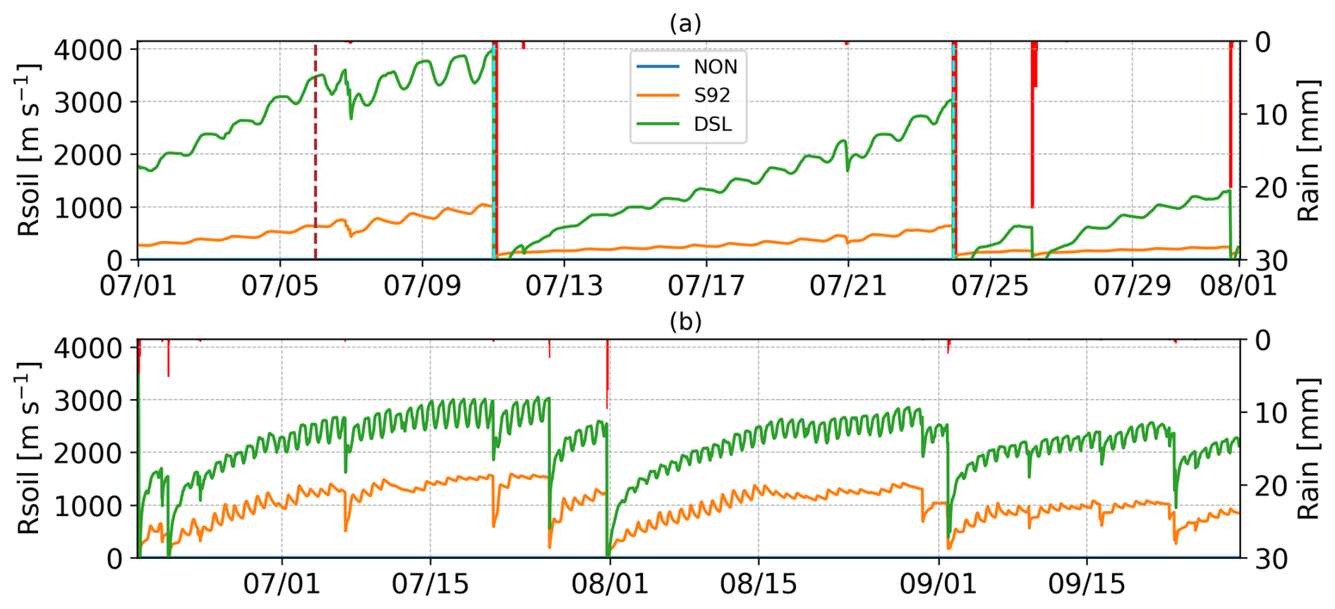
Figure 7Simulated soil resistance timeseries of La Cendrosa (a) and for Els Plans sites (b) for the simulations with no resistance (NON, blue), with a Sellers 92 resistance (S92, orange) and with a DSL resistance (DSL, green). Bar lines represent the rain. Vertical lines represent the vegetation cut (brown) and irrigation (cyan).
In the case of Els Plans, the resistance values of the DSL simulation remained continuously above the value of S92, and increased by a factor of almost 2 (Fig. 7b). Generally, rainfall events were not abundant enough during the summer season, when the evaporative demand was high, to reduce the resistances to zero at this site. Although the resistances were significantly reduced at times, the arid conditions were persistent throughout the summer months.
The estimated resistance values for Els Plans are similar to those found in Swenson and Lawrence (2014), while those of La Cendrosa are higher, due to the differences in soil properties. The increase in resistance starts earlier than observed in laboratory studies (Zhang et al., 2015). Their values were closer to the S92 simulation, but slightly higher and remained lower than those shown for the DSL simulation. These differences result in limited change in LE as there's little water available in the soil, since the VWC is much lower than the field capacity. In addition, Balugani et al. (2023) found that a DSL observed under natural conditions can be larger than that measured in a lysimeter, whether in laboratory or field conditions. The higher resistance values compared to those in Zhang et al. (2015) may be explained by the exposition to the atmospheric conditions which will affect ET, soil moisture and soil temperature profile (Balugani et al., 2023). To explore this further, the following section carries out a sensitivity analysis to test the optimal parameter configuration.
5.2.2 Water Storage
To study the longer term effects of using a soil resistance, Fig. 8a shows the cumulative water loss and its decomposition into transpiration and soil evaporation at La Cendrosa. The differences in cummulative E loss between the various simulations are small before the vegetation is cut, up to 3 mm (2 %). The LE is underestimated in all three simulations and the simulated transpiration dominates until the alfalfa harvest on 6 July. Thereafter, a first trend change is observed, which is reproduced by all three simulations. After the irrigation event of the 11 July, a second change in tendency occurs for which transpiration increases slightly, but soil evaporation increases significantly the following days. The strength of this increase is determined by the resistance applied to the simulation (Fig. 7). The LE in the DSL simulation initially underestimates E slightly, but it recovers during the growth period and matches the E trend at the end of the period, falling within 1 mm difference with respect to observations. The other two simulations accumulate an excess water loss of 9 mm for S92 and 19 mm for NON due to overestimating of bare soil evaporation. Estimation of the partitioning can be made for 29 July at this site as an estimate of the ratio between transpiration and ET for daytime was made on 29 July using microlysimeter and EC measurements. The observation gives a ratio of 0.87 for this day. Simulations using DSL produced the closest ratios to the observations, with a ratio of 0.88. The NON simulations resulted in a much lower ratio (0.66), showing that the contribution of soil evaporation to total ET is significantly overestimated without DSL. However, it should be noted that the NON simulations can reach values up to 0.85 for other days.
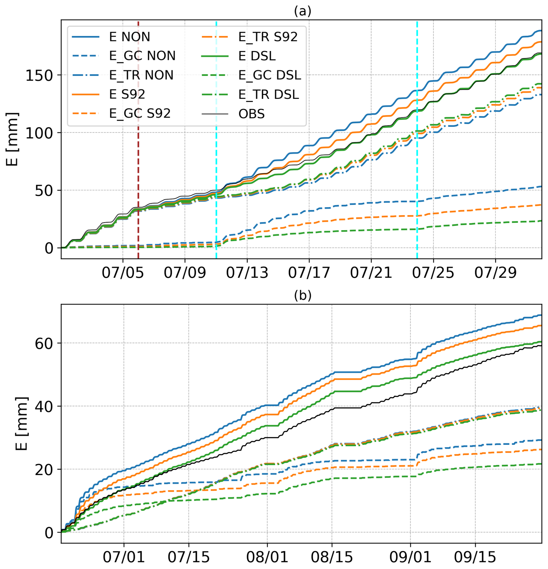
Figure 8Accumulated latent heat flux (E) for La Cendrosa (a) and Els Plans sites (b). Observations are in black, simulations with no resistance are in blue, with Sellers 92 in orange and a DSL resistance in green. Solid lines correspond to the E, dashed lines correspond to the ground evaporation and dashed and dotted lines correspond to the transpiration contribution. The vertical brown line corresponds to the harvest, and cyan lines correspond to irrigation events.
For the four months analyzed at Els Plans, the minimum cumulative change was determined to be in July. After a significant rain event in early August, the E rate increased as more water was available. Figure 8b shows the E and the partitioning of the model. It is important to note that we are at the limits of the model for representing LE with the current LAI formulation of SURFEX. LAI is used to represent the density of photosynthetically active vegetation. For this site, there was a shading effect and the thermal inertia due to the vegetation mass was high, but a very limited transpiration. These effects are not well taken into account due to their dependence on LAI and its low value to represent the small part of active vegetation. Thus, the model also accentuates the soil flux for this site.
Despite these difficulties, the simulation with a DSL manages to reproduce the cumulative evaporated water at the beginning of the period and largely matches the tendency during the summer months. The split between transpiration and bare soil evaporation may be biased towards more transpiration than occurred in reality as estimations of LE in similar conditions can be of only 10 % (Ma et al., 2020), but they are within the realm of possibility as senescent leaves have been reported to be limited to transpiration of 0.1 mm h−1 (Pérez-Anta et al., 2024). Gaps in the LE measurements during the rainy period prevented observation of the increase in cumulative evaporated water during periods with infiltration. The cumulative water during the driest period near the 15 July was underestimated by 4 mm and by 10 mm for the DSL and NON simulations, respectively, during the SOP. At the end of September, the cumulative evaporated water overestimation is slightly reduced to 1 and 9 mm for the DSL and NON simulations, respectively. A small amount of resilient vegetation was observed to germinate at the end of August, which may explain the additional LE and reduction of the model bias. The LE values for this period are low enough that the observational uncertainty of LE can explain a large part of these differences. Nevertheless, it is noteworthy that the change in the trend of evaporation in August in the observations corresponds with the beginning of sporadic natural grasses at the Els Plans site.
When comparing the two sites, the difference in the amount of water evaporated between the two sites is remarkable. In one month at La Cendrosa, the amount of water evaporated is three times greater than that accumulated in more than three months at Els Plans: irrigation significantly alters the water balance of the area.
5.3 Other relevant variables
5.3.1 Albedo
The observed daily variability of albedo and its model counterpart are shown for La Cendrosa in Fig. 9a. The standard deviation shown is from the 30 min time series of the observations and the simulation. Observed albedo values varied by more than 0.1 during the month of July. The alfalfa albedo variability has been reported to be up to 0.2, depending on the solar angle (Al-Yemeni and Grace, 1995). The change is linked to alfalfa leaves which track the solar angle: they cup and reduce the albedo (Travis and Reed, 1983). This process occurs in conjunction with a midday decrease in leaf water potential (Bell et al., 2007).
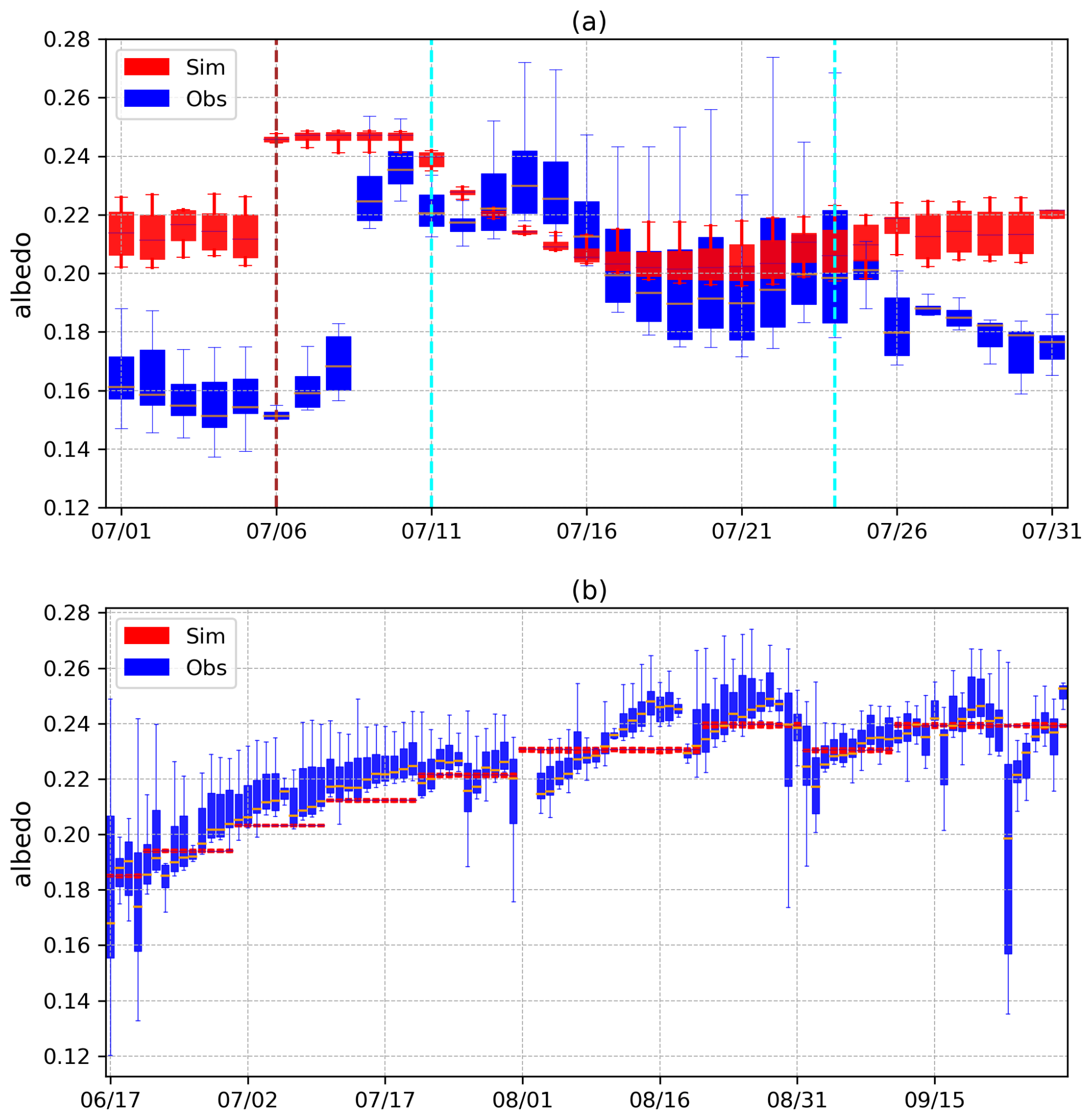
Figure 9Observed (blue) and simulated (red) albedo for the NON simulation for La Cendrosa (a) and Els Plans sites (b). Each boxplot measurement shows a central line with the median value. The size of the boxes correspond to the quartiles of albedo observations within the day and the error bars to the variability of the albedo within the day.
The model albedo is obtained through a constant imposed value for both surface albedo and vegetation albedo. It was chosen to provide a more accurate Rn so that the available energy of the model remained accurate for the other fluxes. ISBA-MEB modifies this initial value by taking into account LAI and the solar zenith angle. The model reproduced then part of the cycle, but its amplitude was weaker than the measured one, changing by at most 0.03. Observations show that alfalfa has albedo values close to 0.16 when fully grown, while after cutting the surface albedo increases to values close to 0.22 and varies with vegetation growth and VWC. As albedo was forced with daily varying values in the current study, modelling the absorption in MEB through the canopy captures some of the changes due to growth from the 9th to the second irrigation period, the 24th. In Fig. 9b, the albedo of Els Plans is influenced by the dryness of the soil, varying with the formation of the DSL and the reduction in VWC in accordance to what De Silans et al. (1989) and Van de Griend and Owe (1994) have observed under bare soil semiarid conditions. The change in albedo over the LOP ranged from 0.18 to 0.25, which is consistent with the findings of Béziat et al. (2013), who found an albedo of 0.25 for senescent crops which are expected to be close to senescent natural grass. Observed rain events reduced soil albedo by up to 0.03 between the events and the periods before and after them. The decadal prescription of the albedo is not enough to capture this variation. Due to the low LAI, no daily cycle is included in the simulation of Els Plans although a sub-daily variability of albedo is observed. These differences do not generate a large discrepancy in the Rn.
5.3.2 Volumetric water content
The VWC dynamics are closely tied to LE, and ISBA attempts to represent this linkage through several mechanisms. The amount of transpiration is limited by Dmax, Eq. (A6), through the water stress factor f2 in Eq. (A8), and bare soil evaporation by VWC, Eq. (3). Adding a soil resistance, such as DSL resistance, introduces an additional dependence of LE on VWC, which limits further ET when VWC is scarce.
Reproduction of VWC dynamics is highly dependent on soil hydraulic properties obtained for the site La Cendrosa from soil texture data and a pedotransfer function. The observations of VWC at La Cendrosa (Fig. 10a) present a soil moisture profile that does not decrease with depth. Rather, there is a layer at 10 cm that reacts very quickly to precipitation or irrigation events. This indicates that drainage after precipitation or irrigation is significantly faster than for observations at depth of 5 or 30 cm. This layer has a much higher sand content which, combined with a lower field capacity and a higher Ksat, results in faster infiltration of water into deeper soil layers. This layer seems to coincide with the point at which the number of roots begins to decrease, as seen when the sensors were installed. This could mean that in drier conditions in the topsoil (−5 cm), root water uptake can decrease rapidly. Soil samples were taken at depths of 0 to 10 cm and 10 to 30 cm and the analysis data (Table 1) show that there is a strong change in sand content and Ksat at 10 cm depth. The large difference in the observed VWC and drainage dynamics after the events suggests that the probe represents the depth between 10 and 30 cm. The rapid response of the VWC during rainfall and irrigation events might indicate that water was transferred along spatially distinct pathways (preferential flow) in the soil subsurface (Guo and Lin, 2018).
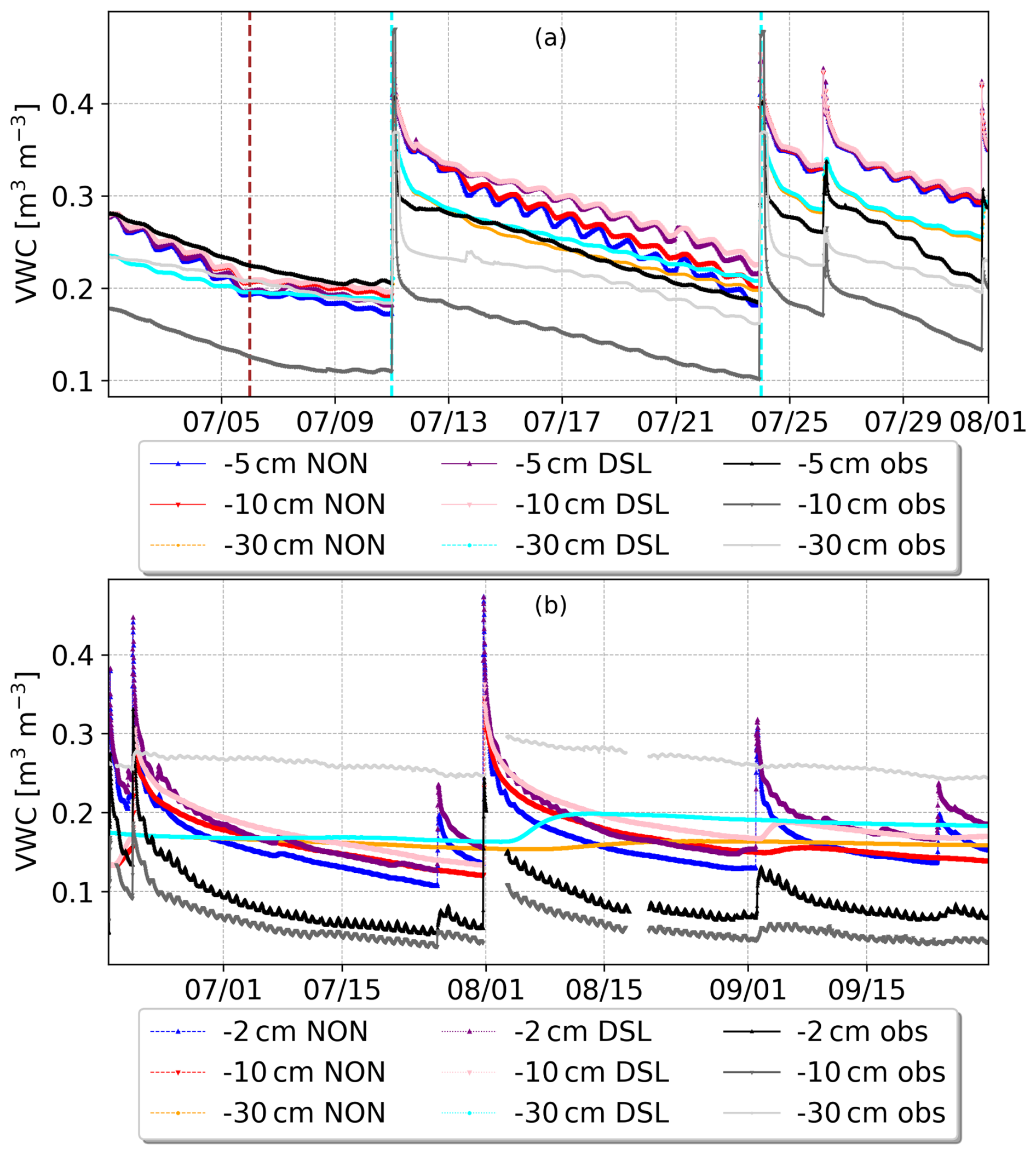
Figure 10Volumetric water content (VWC) of the soil at La Cendrosa site (a) and Els Plans (b) sites at different depths. Levels comprise 2 or 5 (upward triangles) depending on the availability for the site, 10 (downward triangles) and 30 cm (circles). Respectively, observed VWC is shown in black, dark grey and light grey lines, the NON simulation in dark blue, red and orange dashed lines and the DSL simulation in purple, pink and cyan dotted lines.
The VWC in ISBA is simulated using the mixed-form of the Richardson equation, and can therefore model heterogeneous vertical texture or soil property profiles. In the current study, it was found that changing the soil hydraulic parameters to represent the uppermost five layers (0–13.5 cm) to have a higher sand content at the first two layers and lower for the other three significantly impacts the soil properties, and the observed profile with a more humid 10 cm level can be better reproduced (not shown). Current soil world databases predict the superficial layer up to 5 cm to a resolution of 250 m (Hengl et al., 2017) and are used by multiple global models (Vereecken et al., 2019). But as seen by the difference in sand content between the two surface soil surface layer measurements from Table 2, the spatial variability of the soil is high at this site. Measurements within the field close to the EC-tower showed a much higher sand content (56 %) for the top layer (0–10 cm) compared to the observations at another location in the same field (38 %) from Table 2. In consequence, the parameters have been left as those indicated in Table 2.
The La Cendrosa simulation exhibits a 5 % positive bias in VWC during irrigation flood events caused by a lack of drainage, but the model is able to capture the tendency of the VWC for the DSL simulation. Note that for the NON simulation, this tendency is underestimated. Although the absolute value is closer to observation for the period before 24 July, the rate of loss of water has to be correct for proper LE estimation, and it is thus prioritized over absolute value, which is driven by the field capacity value and which has been calculated with soil samples with CH78 pedotransfer functions. Furthermore, the values of VWC probes can be subject to biases due to the type of probe and manufacturing (Jackisch et al., 2020). The rapid response of the water content at all three observation depths following the flood irrigation event probably indicates that some of the water is being transferred to deeper soil levels via preferential flow pathways in macropores (Nimmo et al., 2025). Implementing a dual permeability approach, as described by (Gerke and Van Genuchten, 1993), could improve the simulation of water flow using the Richards equation in fractures (macropores) and the matrix (micropores) in the future but such changes still face challenges for the implementation at larger scales. After 24 July, when the vegetation is almost fully developed, the differences between these simulations remain small, but the differences against observation remain large.
For Els Plans (Fig. 10b), the same bias is observed in terms of the trend. The absolute value of the NON simulation is closer to the observation for 5 and 10 cm, but it deviates significantly from the observation for 30 cm. Here, the DSL appears to more accurately capture the redistribution of water following a rainfall event than the NON, as too much water is used in this approach for soil evaporation. The tendency is larger for the NON simulation than for the observation. For the DSL the tendency is too strong on the wetting events, following what was observed for LE, and giving further necessity for a sensitivity test of the resistance. The difference between the simulations becomes increasingly larger for each soil water content level, which are reduced after rain events. The re-wetting of the deeper layer (i.e., 30 cm) only occurs for the largest rainfall event on the 31 July as a delayed response, since the top soil layer was very dry. Water was mainly used to refill the soil water storage, so it could not infiltrate deeper than 10 cm for the other events. The simulations showed a delayed response compared to the observations when water infiltrated to the 30 cm layer.
Despite the more extensive measurements of soil hydraulic parameters, some potentially important processes, such as flows through cracks or macropores (preferential flow paths) are currently not included in the model structure. In general, the use of pedotransfer functions or laboratory measurements may not be suitable for determining soil hydraulic properties for a specific site. Weihermüller et al. (2021) showed that the choice of pedotransfer function can have a large impact on soil water dynamics, so using an ensemble mean instead of a specific pedotransfer function can be a good solution to reduce this uncertainty (e.g. Krevh et al., 2023). A better method is the inverse estimation of soil hydraulic parameters based on observations of soil water dynamics for the different layers, which significantly reduces this parameter uncertainty. However, this method requires sufficient in situ observations of VWC and matric potential (Groh et al., 2018b; Schübl et al., 2023), which determine the field water retention characteristic, as well as sufficiently long time series that include drying and re-wetting phases. A study of this kind was carried out with SURFEX v8.1 by Sobaga et al. (2023), in which drainage was assessed and improved. Its functions are still being migrated to V9, so the observational derived parameters were given priority in this study.
5.3.3 Soil temperature
The diurnal cycle of soil temperature measured at a depth of 5 cm in La Cendrosa (Fig. 11a) has an amplitude of approximately 5 °C on most days. Before irrigation, when the vegetation is very low, it reaches a maximum of about 10 °C. In contrast, the simulations have a larger amplitude at the beginning. After irrigation, the NON simulation better reproduces the soil temperature diurnal pattern. The DSL simulation increases the temperature at 5 cm up to 5 °C in response to the increase in G due to the decrease in LE. The interaction between the atmosphere and the ground is insufficient and heat is stored instead of being transformed into sensible heat. While the roughness length could be increased to reduce this effect, the characterization of LE would be impacted negatively. For Els Plans, Fig. 11b shows a period of drying. At the beginning, when water is more available, the differences between the NON and the DSL simulations was up to 2 °C, leveling off when soil moisture at the surface layer reduces over time. The layers below 5 cm show the greatest differences, while the temperature at 10 cm maintains a maximum difference of 5 °C throughout the period. These differences indicate that the thermal conductivity is too high. Attempts to reduce the amplitude of soil temperature, such as the inclusion of the impact of soil organic matter on the soil thermal properties, reduce the bias but do not completely correct it and do not correspond to a realistic characterization of the soil at the site. In order to remain as close as possible to the real behavior of the global application of the model, no change has been made to the thermal conductivity. Strategies such as a variable thermal conductivity of the first layer dependent on its thickness such as for the CLM model (Swenson and Lawrence, 2014) could be adopted if a pattern is identified for larger domains.
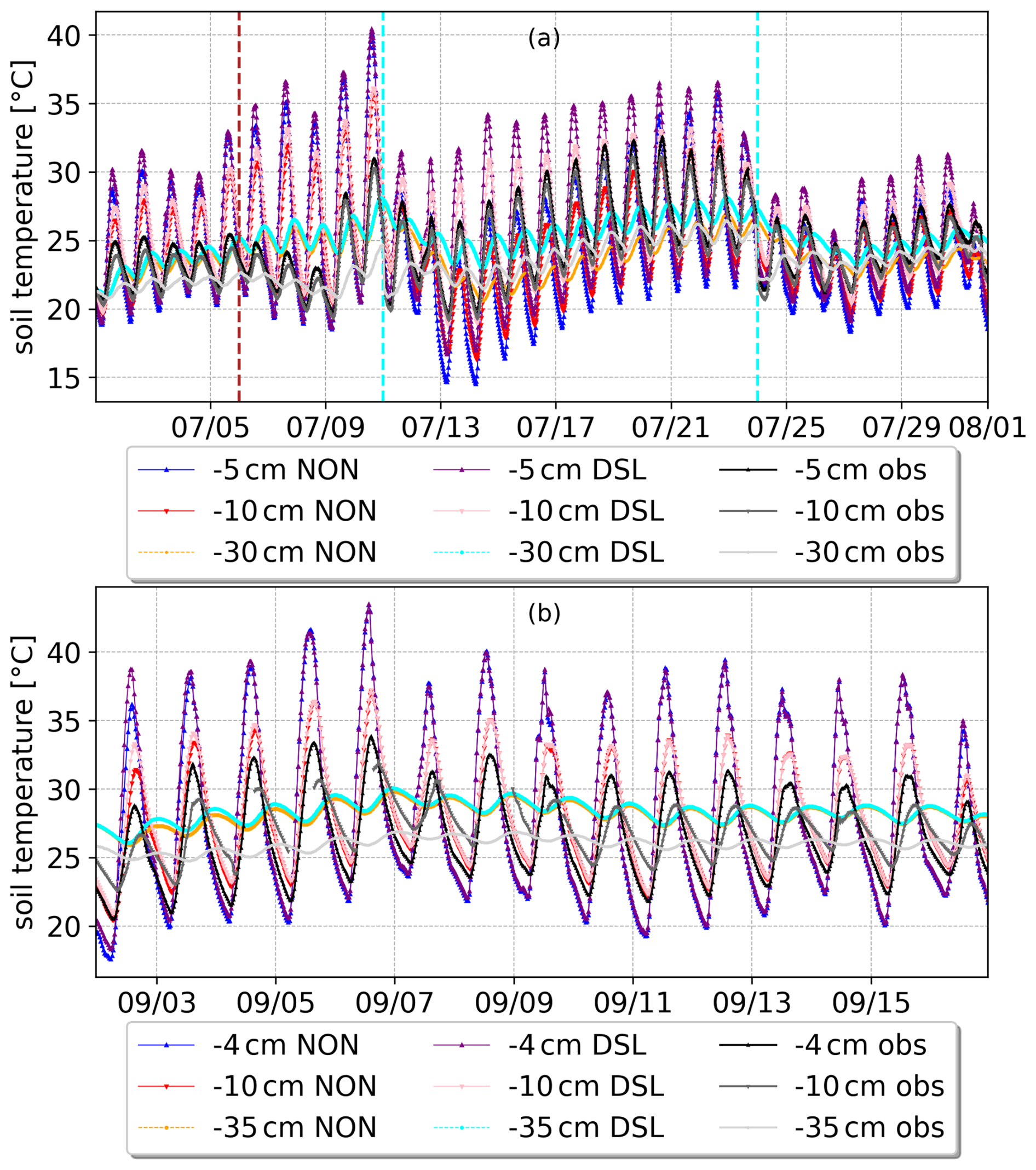
Figure 11Soil temperature at La Cendrosa site (a) and Els Plans (b). Levels comprise at 4 or 5 (upward triangles), 10 (downward triangles), 30 or 35 cm (circles) depending on the availability for the site. Respectively, observed VWC is shown in black, dark grey and light grey lines, the NON simulation in dark blue, red and orange dashed lines and the DSL simulation in purple, pink and cyan dotted lines.
5.4 Parameter sensitivity analysis
The parametrization of DSL resistance depends on parameters with uncertain values because DSL formation depends on soil type and other soil properties that are often unknown. The parameters Kdsl and zdsl are assumed to be the most important since small variations can change the global ET (Swenson and Lawrence, 2014) by over 10 % as they modulate the onset of a DSL and the rate of its growth, respectively. Therefore, a sensitivity analysis of Kdsl and zdsl was performed for both sites during the daytime since this is when the ground resistance should have the largest impact on ET. The RMSE of the estimated fluxes for La Cendrosa (a, c, e, g) and Els Plans (b, d, f, h) for a range of values of zdsl and Kdsl during the daytime is shown in Fig. 12 for the approach with an DSL. Changes in zdsl produce a linear effect as the resistance changes in magnitude, whereas the effect produced by changes in Kdsl is non-linear and it is proportional to the soil's saturation value.
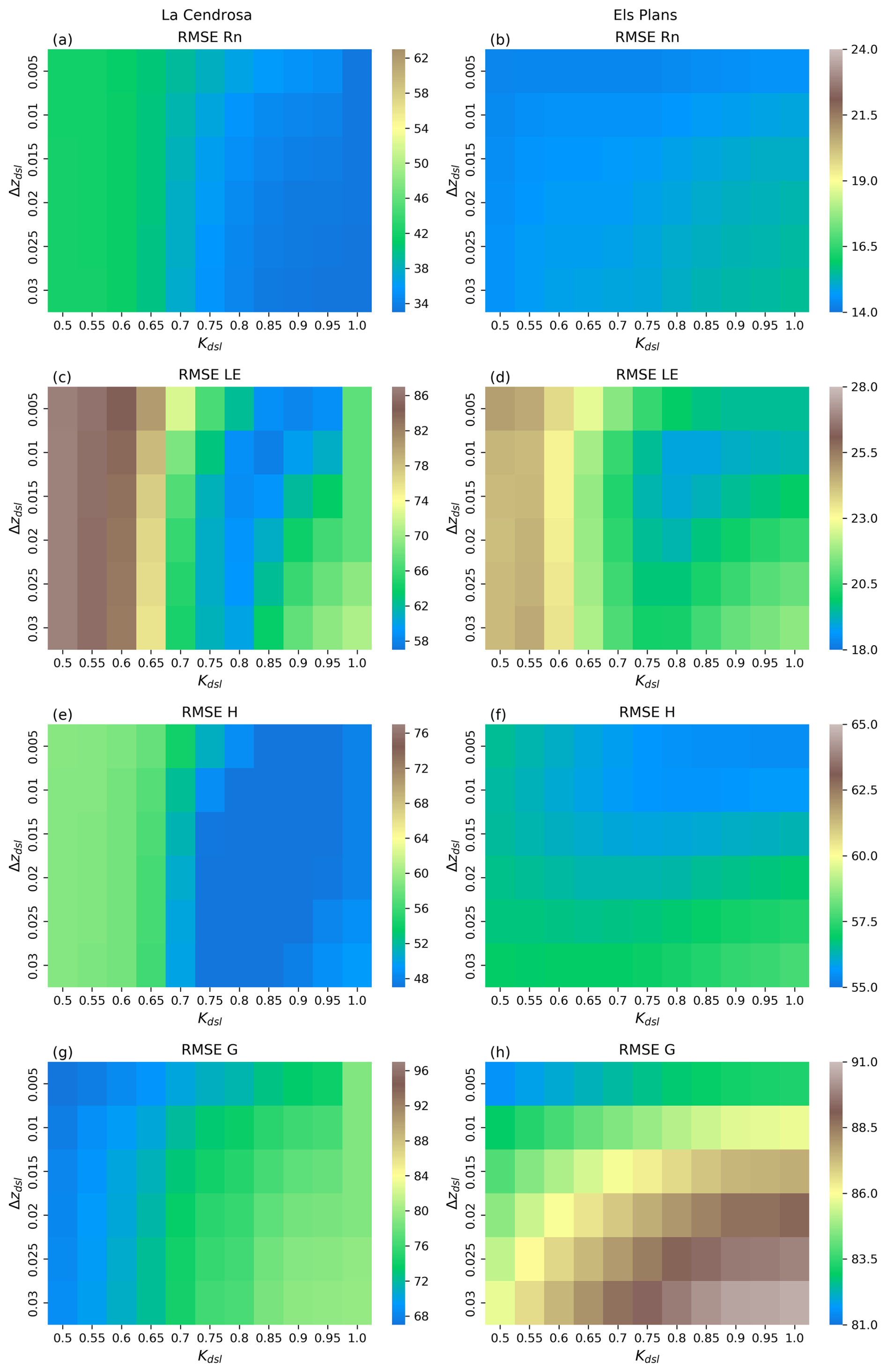
Figure 12Parameter sensitivity test for the energy budget terms modifying Kdsl and zdsl with a DSL resistance for La Cendrosa site [left] and Els Plans [right] during the day. The color represents the resulting RMSE for the daytime for Rn (a), LE (b), H (c), G (d).
For Rn, the optimal values of RMSE for La Cendrosa and Els Plans in Fig. 12a and b are at the opposite extremes of the tested sensitivity values. The RMSE value comparing the default DSL simulation shown in the previous section to the optimal value is very low, between 4 W m−2 for La Cendrosa and 2 W m−2 for Els Plans.
For La Cendrosa, the improvement with higher resistance comes from the days after the irrigation period, when the Rn is overestimated and the decrease in LE is compensated by a rise in H and G together with a reduction of the longwave emission, which reduces the positive bias. For Els Plans, for days when the soil remains dry, the simulation with a larger DSL resistance value shows a greater Rn compared to simulations with a lower resistance value, whereas under humid conditions, the opposite is true. The increase in error in Rn with an increasing resistance value depends on several factors and not on a specific period.
For the LE and H fluxes, it can be observed that values of Kdsl below 0.6 degrade the simulations compared to the proposed DSL values of Swenson and Lawrence (2014) (daytime in Tables 3 and 4). In Sect. 5.1, it was observed that although the DSL simulation produced better results than the simulation without a resistance (NON), the damping of evaporation was greater than optimal for both sites. This is consistent with the sensitivity tests where values of LE with a width resistance of zdsl=0.01 m show the minimum value of RMSE instead of the value found by Swenson and Lawrence (2014). These discrepancies are within what would be expected from the LSM dependence on the characterization of other processes and the use of two contrasting case studies. The error in H is also reduced with a thinner resistance layer. On the other hand, the value of Kdsl seems to be optimal at 0.85, closely followed by 0.8, as the error remains within 1 W m−2, which corresponds to the proposed value of Swenson and Lawrence (2014). Zhang et al. (2015) show resistances appearing at values of Kdsl close to 0.95 for soils with coarser texture (e.g. higher sand content), but in soils with finer texture, the resistance is first estimated at lower values (0.8 to 0.6). The best values for soils with more clay correspond to values of Kdsl of 0.9 or higher, although the resistance has a very small value. A value of Kdsl close to 0.8 should allow enough open pore space for a DSL to fully form.
The use of a DSL resistance results in the storage of excess energy in the soil, so that the optimum value for G in ISBA corresponds to the lowest possible soil resistance. Other soil constituents and processes can alter the thermal properties of the soil and are still to be included in LSMs (Vereecken et al., 2019). To improve this flux in SURFEX, a more detailed investigation of the thermal properties of the soil is still needed, but this is outside of the scope of the current study.
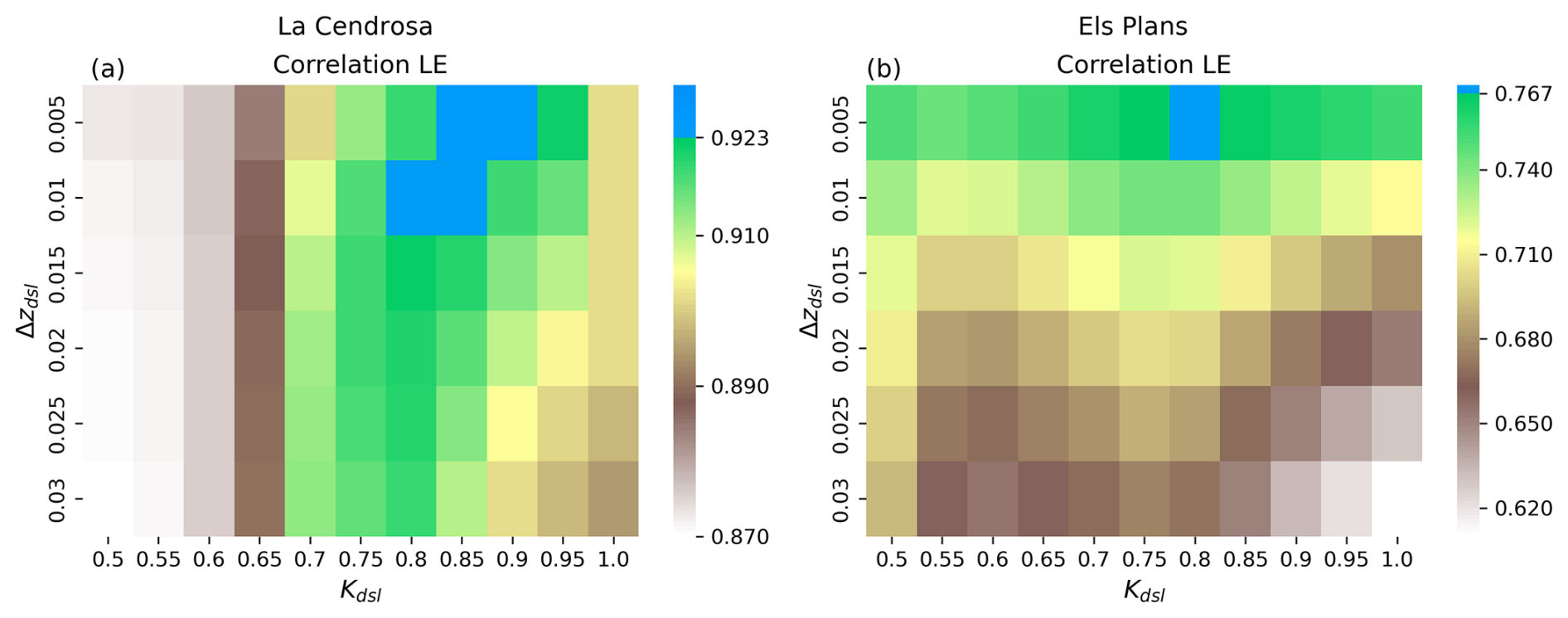
The correlation values of LE for the different values of Kdsl and zdsl are shown in Fig. 13. The correlation for La Cendrosa is improved over the S92 simulation (daytime in Table 3) and for Els Plans it is equal to or slightly better than the NON simulation (daytime in Table 4).This implies that the optimal values for improving LE are zdsl = 0.01 and Kdsl = 0.85. They have a greater resistance than S92 but less than that found in Swenson and Lawrence (2014), for the two sites and specific conditions considered in the current study. At a larger scale, this difference in parameters to Swenson and Lawrence (2014) global runs would imply a smaller resistance generally, except for the development of the resistance which starts at slightly higher soil water contents. Improvement of LE estimation is expected with the application of the DSL resistance at a larger scale. Zhang and Wang (2017) showed that while there are differences between soil types, a resistance exists and it should prove an improvement in other semi-arid sites. Further refinement on these parameters is still possible with larger sampling, particularly in the form of zdsl which presents a linear dependence at this point. The interactions of a soil resistance with different kinds of vegetation have not been been a point of study, largely studied due to technical difficulties: laboratory setup studies would need too many samples and time for the soil to stabilize and studies would tend to use more complex models, in situ meteorological stations do not have systematically the soil characteristics to verify the results. Furthermore, the application of the soil resistance will result in minimal improvement in locations with a very high vegetation transpiration to evaporation ratio contribution.
Estimation of evapotranspiration (ET) in semi-arid environments is continuously improving in LSMs, with ET partitioning being a challenge as there are still few measurements characterizing the components of ET. In this context, two contrasting LIAISE sites were investigated. The default simulations showed an overestimation of ET due to the overestimation of bare soil evaporation, a feature common in multiple LSMs which has been addressed by adding surface resistances of different forms. As a consequence, a soil resistance has been implemented in SURFEX V9 using two options: Sellers 92, a resistance formulation widely used by LSMs that was incorporated in V8, and a newly implemented DSL resistance that more accurately represents the actual physical process modulating bare-soil evaporation. There was an improvement of almost 30 % in RMSE in ET at each site and no degradation of H using the DSL resistance approach. There was an impact on Rn and G which changed mainly due to the increased soil heating owing to reduced LE.
The sites presented several challenges for the model configuration related to vegetation parametrization and management, such as harvesting and irrigation. The first site consisted in an alfalfa field named La Cendrosa, where a detailed characterization of the crop and its biophysical parameters has been made. Such efforts can be later transformed into an informed decision on approximations on a global scale for similar crop types and climates. The development of alfalfa was represented taking into account a daily evolution of LAI and vegetation height based on observations. The study of the photosynthesis parameters used to configure the simulation has shown that the model is sensitive to the cuticular conductance, although it is not the driving mechanism. Instead, the increase in quantum efficiency and the assimilation parameter are most responsible for the increase in ET for alfalfa. These measurements and their parameterization in the model are considered to have improved the estimation of transpiration. Using a relatively accurate parameter set for photosynthesis and without the presence of the crop after cutting, the DSL resistance becomes important in maintaining the correct amount of bare soil evaporation. The daytime ME and RSME for LE were both reduced by approximately 30 W m−2 and the correlation increased from 0.87 to 0.92 when using a DSL, whereas the improvement on H and Rn is of a change in ME and RMSE together of 8 W m−2, the same order as the degradation of G.
The second site corresponds to a rain-fed natural dry grassland named Els Plans. An almost continuous DSL resistance together with a very low LAI maintains the very low LE fluxes which is consistent with those observed by the eddy covariance system. The differences for LE in the rate of drying after each rain event point to other processes being involved such as wind speed or air saturation. The DSL resistance produced a similar improvement to that observed at the La Cendrosa site, but with a reduction in the correlation of LE. Two factors played a role: the limitations of a low LAI to characterize vegetation at Els Plans site, and a resistance value that does not account for the internal biases of the ISBA model at both sites, which led to the need for sensitivity tests.
The parameter sensitivity analysis for the DSL resistance approach suggests a slightly lower zdsl value for the two sites used in the current study than the value found in Swenson and Lawrence (2014). The correlation of LE increased by 0.01 for La Cendrosa compared to the initial value of zdsl. The correlation with the new values compared to the initial NON simulation was increased by 0.02 at La Cendrosa and is left neutral for Els Plans. The overall error of the simulation was also reduced. The resistance value from the DSL approach was still greater than that obtained when using the S92 method. The point at which resistance begins to develop has been found to be when approximately twenty percent of the available space in the first layer has been occupied by air.
In addition, the analysis of the two sites has also considered their soil properties, as the DSL involves changes in soil temperature and soil water content. The increase in soil temperature is greater when moisture and bare soil evaporation are significant and the DSL is still present. Laboratory based soil hydraulic properties were available but were found to be insufficient to reproduce the VWC, a behavior also reported in Aouade et al. (2020). Therefore, it is recommended that further studies include variables that define the soil water retention characteristics when calibrating the model.
Finally, the DSL parametrization provides a plausible physical interpretation of the simulated evaporation which is lower than in the baseline scheme while remaining pragmatic since the equation does not explicitly represent water vapor transport. We have shown that it can be applied to conditions that represent the extremes of a semi-arid environment and under different land management practices, including flood irrigation. A multi-site or a global/regional analysis should help to define the choice of parameters for more climates and land cover types. Values with a Kdsl between 0.8 and 0.85 and a zdsl near 0.01 m were found for the two sites used in the current study remaining near 0.8 and lower while close to the 0.015 m of Swenson and Lawrence (2014). The DSL resistance methodology seems to be rather robust since similar parameter values are obtained between two different LSMs and varying surface conditions.
A1 Components of the vegetation latent heat flux
The components of the vegetation water exchange Ev are given by:
and
with where gsI is the stomatal conductance at the canopy level and it is the weighted average of the different plant types multiplied by the LAI, ρa is the air density, qsat,v is the saturated specific content at the vegetation temperature and qc is the canopy air specific humidity (kg kg−1). Ravg-c is the resistance between the overlaying air and vegetation. It consists on the inverse of the sum of the bulk canopy aerodynamic conductance between the canopy and the canopy air (Choudhury and Monteith, 1988) and the conductance accounting for the free convection from (Sellers et al., 1986). δ is the Halstead coefficient with a factor to account that saturated vegetation can transpire. See Boone et al. (2017), Sect. 2.6.1 for the particulars of the aerodynamic resistance of the canopy, Sect. 2.8.3 for the Halstead coefficient and their Appendix C2 for the LE formulation, which fall outside the discussions of this article.
A2 A-gs model
A2.1 Transpiration formulation
The A-gs (Assimilation-stomatal conductance) scheme of Goudriaan et al. (1985) within SURFEX presents the parametrization of plant assimilation of carbon. It was modified by Jacobs et al. (1996) to model photosynthesis and it can be used to obtain transpiration. Different types of vegetation can be selected and its parametrizations are modeled as a function of the so-called vegetation patch (or land cover type). In SURFEX, a patch corresponds to a Plant Functional type (PFT), which characterizes subcategories natural land-surfaces. Additionally, vegetation can have either drought tolerant or drought avoidant strategies (Calvet et al., 2004). A description of the processes can be found in Calvet et al. (1998) and Delire et al. (2020).
In order to describe the parameter selection methodology, we provide the mathematical development of the low vegetation scheme in ISBA (Calvet, 2000), which is used to represent crops and herbaceous types in contrast to high vegetation that considers woody types. The main difference is in the relationship between the mesophilic conductance and the maximum humidity deficit. A glossary containing the parameter definitions is provided in Appendix D. Transpiration in A-gs is given by:
Ds is the specific humidity deficit. Ds indicates when stomata are closed by exceeding Dmax, the maximum specific humidity deficit of the air tolerated by the vegetation (with no soil water stress). The stomatal conductance calculation is presented in Appendix A3 for thoroughness. Ds is of the form:
where f indicates the proportionality of internal CO2 inside the leaf boundary layer and is f with no saturation deficit (without soil water stress) and are model parameters (see Table A1). fmin is the minimal value of f:
where is the mesophyllic conductance and gc is the cuticular conductance. determines the gas exchange amount through the stomata and gc through the cuticle when stomata are completely closed, they depend on the plant type rather than on C3 and C4 strategy. The cuticle is a kind of wax membrane that protects the leaf and allows little exchange of gases, its values being smaller than those of . Both contribute to the total transpiration.
A2.2 Evaporation strategies
Dmax behavior varies with evaporation strategy, limiting transpiration depending on its value. The formulation is the following:
where can be N for the drought-avoiding strategy applied for C3 crops (Eq. A7), and X for the drought-tolerant strategy (Eq. A9). Given the same Dmax, transpiration will decrease for C3 and increase for C4 plants under water stress conditions due to these different strategies. For C3 crops is given by:
and
where f2 is the normalized soil moisture and f2c is its tabulated critical value. f2 is summed over the soil layers Ng (Decharme et al., 2011). Soil water content variables are represented by ω. The first subindex indicates the water content variable, g is the ground, wilt is the wilting point and fc is the field capacity. The second subindex corresponds to the layer number to which it pertains, 1 would indicate the most superficial layer. ζi represents the difference in the cumulative root zone fraction for a given layer. Within this strategy Dmax increases until critical soil moisture is reached (f2=f2c), then the previous symbolized by is updated and decreases with the water deficit: .
For the drought tolerant strategy used for C4 crops and in our simulated alfalfa, we take Eq. (A6), with given by:
In this strategy then Dmax increases until the critical soil moisture is reached, Dmax decreases with the severity of the stress: . Note that this is the opposite behavior from C3 crops as and are anticorrelated. The calculation of gs is included in Appendix A3 for thoroughness and to facilitate the interpretation of LE changes: a glossary has been included at the end of the document in Table D1.
A3 Stomatal conductance
Table A1Table of default parametrized values in the A-gs scheme for the used PFT.
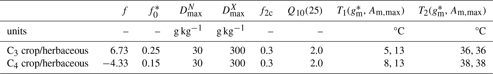
To obtain gs we use the following expressions:
where gsc is the stomatal conductance to CO2 given by:
where Ma and Mv are molecular masses of air and water vapor respectively, Cs is the external concentration of CO2 and Ci the CO2 internal concentration, expressed as:
and
where Γ is the CO2 compensation concentration at the skin temperature, Ts is the superficial temperature of the leaf and Q10 is fixed at 2.0 (see Table A1).
To obtain Efirst with Eq. (A3), accounting for the ratio of CO2 to water assimilation for the stomatal conductance to CO2 with:
where and corresponds to the dark respiration. Am is the CO2 assimilation limited by the air CO2 concentration due to saturation, and An is the CO2 assimilation limited by the air CO2 concentration. Amin represents the residual photosynthesis rate (at full light intensity) associated with cuticular transfers when the stomata are closed because of a high specific humidity deficit, it is expressed as:
where Cmin is the minimum value of Ci at , given by:
Additionally, Am is:
with:
with T1 and T2 being reference temperature values.
where Ia is the photosynthetically active radiation and
where ϵ0 is the quantum efficiency.
The relationships from Eq. (A3) to Eq. (A20) show that gs is highly nonlinear with the parameters , gc, Am,max(25) and ϵ0. Ds is in fact and between others. Discussion on the values of these parameters is done in Sect. 4.2.1 and in further detail Appendix B1.
B1 Vegetation parameterization of alfalfa
A realistic transpiration simulation is essential for obtaining a good estimate of LE, particularly for alfalfa. The process is governed by several parameters that are best prescribed from observational data when available (see Sect. 3.2). We explore them with the AST option within SURFEX in all simulation configurations. With this option, the A-gs scheme is employed to model photosynthesis, parameterizing its processes, in contrast to other options that model transpiration directly without considering the biological processes. The vegetation can exhibit either drought-tolerant, Eq. (A9), or drought-avoidant strategies, Eq. (A7) (Calvet et al., 2004), previously described in Appendix A2.2. The A-gs scheme is rarely compared with direct vegetation measurements (Van Diepen et al., 2022) due to the difficulty of achieving a one-to-one correspondence for the model parameters. Direct observations of stomatal conductance (gs), CO2 assimilation and photosynthetically active radiation (PAR) were obtained at La Cendrosa. The mesophylic () and cuticular conductances (gc), and the maximum assimilation (Am,max(25)) can be found from observations or via the maximum catalytic capacity of Rubisco (Vcmax), the enzyme that controls energy production. In contrast, quantum efficiency (ϵ0) is usually a fitted parameter when the energy, assimilation and carbon curves are measured. After testing multiple parameter configurations, it was found that increasing the quantum efficiency, ϵ0, and the maximum assimilation (Am,max(25)) gave results that reproduce results obtained with a higher cuticular conductance. More energy than the default must be supplied to match the observed fluxes, regardless of whether it comes from the stomata or the cuticle. For this reason, the model adaptations are described below.
-
Mesophyll conductance. The PFT parametrization establishes the through an associated curve that varies depending on whether the water use efficiency strategy under moderate stress is stress tolerant, Eq. (A9), or stress avoidant, Eq. (A7), and only one type is associated with each vegetation type (Calvet, 2000). Although alfalfa is a C3 crop, its drought strategy is tolerant as in C4 crops. Such plants species are known as C4-like species (Way et al., 2014). In consequence, the stress type has been changed to drought tolerant for the simulation. For this site, the highest impact comes from the increase in absolute transpiration and not from the possible changes in stomata closure. With this strategy, parameters are set for generic species and must be modified to represent a particular species. The values have been changed to 0.005 m s−1 (see Table B1). These values are within the observed values of the control (Aranjuelo et al., 2013) and lower values would correspond to stressed alfalfa. Lower values of 0.00197 m s−1 were also observed with unstressed alfalfa (Malik et al., 2018). For the CLASS model (De Arellano et al., 2015), González-Armas et al. (2024) used a value of 0.01 m s−1 which was found for the same site. After setting the other parameters, the differences in mean error and root mean square error modifying the value from 0.005 to 0.1 m s−1 in SURFEX are below 1 W m−2 for all fluxes. Differences arise on the days on which stomatal closure is simulated and depend on what degree the closure is effective. It should be noted that alfalfa is bred for the development of drought/salinity tolerant varieties that are thus optimized for cultivation in arid and semi-arid regions of the Mediterranean area (Mouradi et al., 2022). However, the modification of this parameter is necessary, but there are still errors in the estimation of ET so additional parameters are explored.
-
Cuticular conductance. As a first approximation, increasing the cuticular conductance to 0.0006 m s−1 provided good estimates of ET. Measurements of cuticular conductance can follow several strategies and give different values for the same species (Kerstiens, 1996). Simplification to a minimum value of conductance (gmin) and other similar values such as nocturnal conductance or detached leaf conductance are more commonly measured (Duursma et al., 2019), gmin values are more similar to values of gc which serve as a default in numerical simulations and are used as a proxy. For alfalfa, the value was set to 0.00007 m s−1 according to Kerstiens (1996). When used, it provided simulations with a profound dip in evaporation in the central part of the day, resulting in unrealistic results compared to observations. No further values of gc for alfalfa were found in the literature, which could probably indicate the difficulty of measuring this parameter. The Kerstiens (1996) value is one order of magnitude below the tested value of 0.0006 m s−1 and three times less than the default value in SURFEX of 0.00025 m s−1. The default value has been used as it is closer to the literature value without being outside the typical observed values of this parameter for other vegetation. Values up to at least 0.006 m s−1 can still provide reasonable estimations of ET but are outside the reported values and they are non-physical. This behavior is given by the relationships from Eqs. (A16) and (A5), which holds the sum of gc and in the denominator and can compensate the effects from one another. Together with Eq. (A10), an increase of gc produces a similar effect to increasing .
-
Quantum efficiency. The ϵ0 can be directly related to the increase in transpiration, an increase of ϵ0 in Eq. (A20) induce an increase in carbon assimilation in Eq. (A19) and of the stomatal conductance, Eq. (A10). This parameter is based on the theoretical quantum requirement of photons needed to assimilate one molecule of CO2 (Von Caemmerer and Farquhar, 1981), and it limits the assimilation rate (see review in Van Diepen et al., 2022). Goudriaan et al. (1985) presents a revised value of 0.017 mg CO2 J−1 and suggests that selective breeding of the plant species could lead to an increase in this value in new varieties. Its value has not evolved in the SURFEX configuration over the years. There is some evidence that this value is variable; Collatz et al. (1992) showed a small temperature dependence and Cai and Dang (2002) identified a variability of this parameter within tree species, but the exploration of this parameter in measurements has seemingly not progressed in recent years for meteorological applications. Mouradi et al. (2022) and Jiang et al. (2009) show that depending on the alfalfa variety, the electron transport rate and the PAR conversion efficiency (biological measurements used by their community) can be increased, apparently exploiting an increase in electron efficiency, although no direct conversion to these parameters has been found. This efficiency will decrease during drought events (Zhang et al., 2019; Mouradi et al., 2022). Thus, the ϵ0 value used may be more variable than reported and may have been compensated by an increase in other parameters such as cuticular conductance. The ϵ0 value of 0.0265 mg CO2 J−1 found by González-Armas et al. (2024) increases the LE to values closer to the observed values and is therefore used in this study.
-
Maximum assimilation. The Am,max(25) sensitivity is most relevant for low LAI values, as marginal increases of this value will be weighted more heavily to increase transpiration than for other parameters. The relationship of Am,max in Eq. (A14) has a nonlinear response for gs. The increase of Am,max(25) in Eq. (A18) increases An in Eq. (A19) and on to the stomatal conductance, Eq. (A10), but Am,max can also be found in the denominator.
The default value of Am,max(25) is 2.2 mg. For alfalfa, both higher values (Bunce, 2018) with 2.64 mg, which were transformed from Vcmax as in Collatz et al. (1991), and lower values (Malik et al., 2018) of 1.4 mg have been reported in the literature. González-Armas et al. (2024) found values (3.02 mg) at La Cendrosa that were considerably higher than those given in the literature and the standard value in SURFEX. Increasing this value in this simulation improves the transpiration estimates for days that show a dip in ET during the day reducing its intensity, therefore the value in González-Armas et al. (2024) is kept, but the default values are adequate for most of the simulated days.
Table B1Values for alfalfa of the tested variables of the A-gs configuration in SURFEX. The simulated value corresponds to the final set of parameters used in the results section.
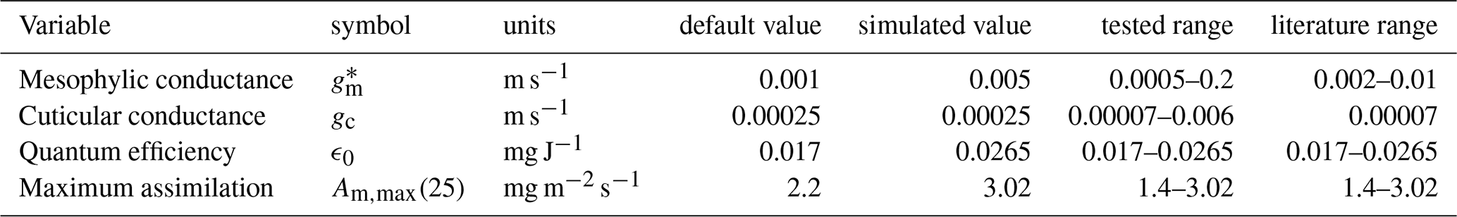
C1 Ground heat flux
The energy budget equation on the SURFEX model can be written as:
where S is the energy storage term and G′ the conduction flux given a particular ground level. G is given then by and it is defined at the surface.
Table D1Glossary table with the variables presented in the article.

a Indicates that the variable is linked to the equation text. b The equations are in ppm but the SURFEX input is in kg m−3.
Table E1Instruments at the selected SEB stations (n/a: not applicable). CSAT3, EC150 and Krypton are Campbell Scientific (CS) Instruments; LI stands for LI-COR, HS-50 and R3-50 are Gill models, CNR1, CNR4, CRg4 and CM21 are Kipp & Zonen devices, the flux plates are made by Hukseflux. There were two SEB stations at La Cendrosa from the CNRM and from WUR.
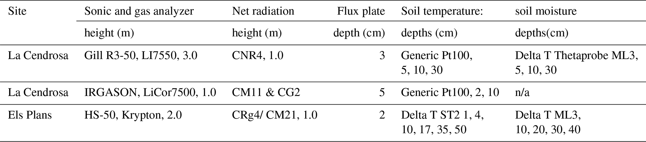
SURFEX is an open source code available at https://www.umr-cnrm.fr/surfex/ (last access: 3 March 2026). The modified routines, the SURFEX version code used and simulations can be found at Martí and Boone (2025): https://doi.org/10.5281/zenodo.15205476. The developed DSL option will be included in following versions of SURFEX. The datasets from the LIAISE campaign are available at https://liaise.aeris-data.fr/page-catalogue/ (last access: 3 March 2026). In particular, the following have been used: https://doi.org/10.25326/320 (Canut, 2022a), https://doi.org/10.25326/430 (Price, 2023) and https://doi.org/10.25326/522 (Brooke, 2023). Additional information of the campaign activities can be found in https://www.hymex.fr/liaise/index.html (last access: 3 March 2026).
BM carried out the development of SURFEX, the preparation of the forcings, the execution and analysis of the simulations and most of the writing and revision of the text. JG participated in the data generation and discussion of the soil properties and reviewed and edited and reviewed the text. GC participated in the data generation and discussion of the surface energy budget data and reviewed the text. AB supervised and advised the work, reviewed and edited the text, provided the necessary funding for the project.
The contact author has declared that none of the authors has any competing interests.
Publisher's note: Copernicus Publications remains neutral with regard to jurisdictional claims made in the text, published maps, institutional affiliations, or any other geographical representation in this paper. The authors bear the ultimate responsibility for providing appropriate place names. Views expressed in the text are those of the authors and do not necessarily reflect the views of the publisher.
We acknowledge Hugo de Boer and Raquel González-Armas for the discussion maintained on A-gs parametrization during the early conception of the article. We acknowledge Oscar Hartogensis and the team of the Wageningen University & Research (WUR) for the alfalfa vegetation measurements. We acknowledge the teams of the Centre National de Recherches Météorologiques (CNRM), the UK Metoffice for the measurements of their energy budget stations. We wish to acknowledge the financial support of the French National Agency for research (grant no. ANR-19-CE01-0017 in support of the project “HILIAISE: Human imprint on Land surface Interactions with the Atmosphere over the Iberian Semi-arid Environment”). Jannis Groh was funded by the Deutsche Forschungsgemeinschaft (DFG, German Research Foundation) – project no. 460817082. We acknowledge the three anonymous reviewers that have revised this manuscript improving its quality.
This research has been supported by the Agence Nationale de la Recherche (grant no. ANR-19-CE01-0017).
This paper was edited by Yongze Song and reviewed by Mousong Wu and two anonymous referees.
Al-Yemeni, M. N. and Grace, J.: Radiation balance of an alfalfa crop in Saudi Arabia, Journal of Arid Environments, 29, 447–454, 1995. a
Alton, P., Fisher, R., Los, S., and Williams, M.: Simulations of global evapotranspiration using semiempirical and mechanistic schemes of plant hydrology, Global Biogeochemical Cycles, 23, https://doi.org/10.1029/2009GB003540, 2009. a
Aouade, G., Jarlan, L., Ezzahar, J., Er-Raki, S., Napoly, A., Benkaddour, A., Khabba, S., Boulet, G., Garrigues, S., Chehbouni, A., and Boone, A.: Evapotranspiration partition using the multiple energy balance version of the ISBA-A-gs land surface model over two irrigated crops in a semi-arid Mediterranean region (Marrakech, Morocco), Hydrol. Earth Syst. Sci., 24, 3789–3814, https://doi.org/10.5194/hess-24-3789-2020, 2020. a, b
Aranjuelo, I., Tcherkez, G., Molero, G., Gilard, F., Avice, J.-C., and Nogués, S.: Concerted changes in N and C primary metabolism in alfalfa (Medicago sativa) under water restriction, Journal of Experimental Botany, 64, 1–17, 2013. a
Aubinet, M., Grelle, A., Ibrom, A., Rannik, Ü., Moncrieff, J., Foken, T., Kowalski, A. S., Martin, P. H., Berbigier, P., Bernhofer, C., Clement, R., Elbers, J., Granier, A., GrÜnwald, T., Morgensten, K., Pilegaard, K., Rebmann, C., Snijders, W., Valentini, R., and Vesala, T.: Estimates of the annual net carbon and water exchange of forests: the EUROFLUX methodology, in: Advances in ecological research, vol. 30, Elsevier, 113–175, https://doi.org/10.1016/S0065-2504(08)60018-5, 2000. a
Balugani, E., Lubczynski, M., Van Der Tol, C., and Metselaar, K.: Testing three approaches to estimate soil evaporation through a dry soil layer in a semi-arid area, Journal of Hydrology, 567, 405–419, 2018. a
Balugani, E., Lubczynski, M., and Metselaar, K.: Evaporation through a dry soil layer: Column experiments, Water Resources Research, 57, e2020WR028286, https://doi.org/10.1029/2020WR028286, 2021. a
Balugani, E., Lubczynski, M., and Metselaar, K.: Lysimeter and in situ field experiments to study soil evaporation through a dry soil layer under semi-arid climate, Water Resources Research, 59, e2022WR033878, https://doi.org/10.1029/2022WR033878, 2023. a, b
Barr, A. G., King, K., Gillespie, T., Den Hartog, G., and Neumann, H.: A comparison of Bowen ratio and eddy correlation sensible and latent heat flux measurements above deciduous forest, Boundary-Layer Meteorology, 71, 21–41, 1994. a
Barton, I.: A parameterization of the evaporation from nonsaturated surfaces, Journal of Applied Meteorology, 18, 43–47, 1979. a
Bell, L. W., Williams, A. H., Ryan, M. H., and Ewing, M. A.: Water relations and adaptations to increasing water deficit in three perennial legumes, Medicago sativa, Dorycnium hirsutum and Dorycnium rectum, Plant and Soil, 290, 231–243, 2007. a
Best, M. J., Pryor, M., Clark, D. B., Rooney, G. G., Essery, R. L. H., Ménard, C. B., Edwards, J. M., Hendry, M. A., Porson, A., Gedney, N., Mercado, L. M., Sitch, S., Blyth, E., Boucher, O., Cox, P. M., Grimmond, C. S. B., and Harding, R. J.: The Joint UK Land Environment Simulator (JULES), model description – Part 1: Energy and water fluxes, Geosci. Model Dev., 4, 677–699, https://doi.org/10.5194/gmd-4-677-2011, 2011. a
Béziat, P., Rivalland, V., Tallec, T., Jarosz, N., Boulet, G., Gentine, P., and Ceschia, E.: Evaluation of a simple approach for crop evapotranspiration partitioning and analysis of the water budget distribution for several crop species, Agricultural and Forest Meteorology, 177, 46–56, 2013. a, b
Boone, A., Samuelsson, P., Gollvik, S., Napoly, A., Jarlan, L., Brun, E., and Decharme, B.: The interactions between soil–biosphere–atmosphere land surface model with a multi-energy balance (ISBA-MEB) option in SURFEXv8 – Part 1: Model description, Geosci. Model Dev., 10, 843–872, https://doi.org/10.5194/gmd-10-843-2017, 2017. a, b, c
Boone, A., Bellvert, J., Best, M., Brooke, J. K., Canut-Rocafort, G., Cuxart, J., Hartogensis, O., Le Moigne, P., Miró, J. R., Polcher, J., Price, J., Quintana Seguí, P., Bech, J., Bezombes, Y., Branch, O., Cristóbal, J., Dassas, K., Fanise, P., Gibert, F., Goulas, Y., Groh, J., Hanus, J., Hmimina, G., Jarlan, L., Kim, E., Le Dantec, V., Le Page, M., Lohou, F., Lothon, M., Mangan, M. R., Martí, B., Martínez-Villagrasa, D., McGregor, J., Kerr-Munslow, A., Ouaadi, N., Philibert, A., Quiros-Vargas, J., Rascher, U., Siegmann, B., Udina, M., Vial, A., Wrenger, B., Wulfmeyer, V., and Zribi, M.: The Land Surface Interactions with the Atmosphere over the Iberian Semi-Arid Environment (LIAISE) Field Campaign, Journal of the European Meteorological Society, 2, 100007, https://doi.org/10.1016/j.jemets.2025.100007, 2025. a, b, c, d
Brooke, J.: LIAISE_ELS-PLANS_UKMO_LAI_01DAY_L1, Aeris [data set], https://doi.org/10.25326/522, 2023. a, b
Brooke, J., Best, M., Lock, A., Osborne, S., Price, J., Cuxart, J., Boone, A., Canut-Rocafort, G., Hartogensis, O., and Roy, A.: Irrigation contrasts through the morning transition, Quarterly Journal of the Royal Meteorological Society, https://doi.org/10.1002/qj.4590, 2023. a, b
Brut, A., Rüdiger, C., Lafont, S., Roujean, J.-L., Calvet, J.-C., Jarlan, L., Gibelin, A.-L., Albergel, C., Le Moigne, P., Soussana, J.-F., Klumpp, K., Guyon, D., Wigneron, J.-P., and Ceschia, E.: Modelling LAI at a regional scale with ISBA-A-gs: comparison with satellite-derived LAI over southwestern France, Biogeosciences, 6, 1389–1404, https://doi.org/10.5194/bg-6-1389-2009, 2009. a
Brutsaert, W.: On a derivable formula for long-wave radiation from clear skies, Water Resources Research, 11, 742–744, 1975. a
Bunce, J.: Thermal acclimation of the temperature dependence of the VCmax of Rubisco in quinoa, Photosynthetica, 56, 1171–1176, 2018. a
Cai, T. and Dang, Q.-L.: Effects of soil temperature on parameters of a coupled photosynthesis–stomatal conductance model, Tree Physiology, 22, 819–828, 2002. a
Calvet, J.-C.: Investigating soil and atmospheric plant water stress using physiological and micrometeorological data, Agricultural and Forest Meteorology, 103, 229–247, 2000. a, b
Calvet, J.-C., Noilhan, J., Roujean, J.-L., Bessemoulin, P., Cabelguenne, M., Olioso, A., and Wigneron, J.-P.: An interactive vegetation SVAT model tested against data from six contrasting sites, Agricultural and Forest Meteorology, 92, 73–95, 1998. a
Calvet, J.-C., Rivalland, V., Picon-Cochard, C., and Guehl, J.-M.: Modelling forest transpiration and CO2 fluxes – Response to soil moisture stress, Agricultural and Forest Meteorology, 124, 143–156, 2004. a, b, c
Camillo, P. J. and Gurney, R. J.: A resistance parameter for bare-soil evaporation models, Soil Science, 141, 95–105, 1986. a
Canut, G.: LIAISE_LA-CENDROSA_CNRM_MTO-FLUX-30MIN_L2 Aeris [data set], https://doi.org/10.25326/320, 2022a. a, b, c
Canut, G.: LIAISE_PREIXANA_CNRM_MTO-FLUX-30MIN_L2, Aeris [data set], https://doi.org/10.25326/361, 2022b. a
Chang, L.-L., Dwivedi, R., Knowles, J. F., Fang, Y.-H., Niu, G.-Y., Pelletier, J. D., Rasmussen, C., Durcik, M., Barron-Gafford, G. A., and Meixner, T.: Why do large-scale land surface models produce a low ratio of transpiration to evapotranspiration?, Journal of Geophysical Research: Atmospheres, 123, 9109–9130, 2018. a, b
Chanzy, A., Mumen, M., and Richard, G.: Accuracy of top soil moisture simulation using a mechanistic model with limited soil characterization, Water Resources Research, 44, https://doi.org/10.1029/2006WR005765, 2008. a
Choudhury, B. J. and Monteith, J.: A four-layer model for the heat budget of homogeneous land surfaces, Quarterly Journal of the Royal Meteorological Society, 114, 373–398, 1988. a
Clapp, R. B. and Hornberger, G. M.: Empirical equations for some soil hydraulic properties, Water Resources Research, 14, 601–604, 1978. a
Coenders-Gerrits, A., Van der Ent, R., Bogaard, T., Wang-Erlandsson, L., Hrachowitz, M., and Savenije, H.: Uncertainties in transpiration estimates, Nature, 506, https://doi.org/10.1038/nature12925, 2014. a
Collatz, G. J., Ball, J. T., Grivet, C., and Berry, J. A.: Physiological and environmental regulation of stomatal conductance, photosynthesis and transpiration: a model that includes a laminar boundary layer, Agricultural and Forest Meteorology, 54, 107–136, 1991. a
Collatz, G. J., Ribas-Carbo, M., and Berry, J. A.: Coupled photosynthesis-stomatal conductance model for leaves of C4 plants, Functional Plant Biology, 19, 519–538, 1992. a
Coudert, B., Ottlé, C., Boudevillain, B., Demarty, J., and Guillevic, P.: Contribution of thermal infrared remote sensing data in multiobjective calibration of a dual-source SVAT model, Journal of Hydrometeorology, 7, 404–420, 2006. a
Cuntz, M., Mai, J., Samaniego, L., Clark, M., Wulfmeyer, V., Branch, O., Attinger, S., and Thober, S.: The impact of standard and hard-coded parameters on the hydrologic fluxes in the Noah-MP land surface model, Journal of Geophysical Research: Atmospheres, 121, 10–676, 2016. a
Cuxart, J., Conangla, L., and Jiménez, M.: Evaluation of the surface energy budget equation with experimental data and the ECMWF model in the Ebro Valley, Journal of Geophysical Research: Atmospheres, 120, 1008–1022, 2015. a
Dare-Idowu, O., Jarlan, L., Le-Dantec, V., Rivalland, V., Ceschia, E., Boone, A., and Brut, A.: Hydrological Functioning of maize crops in Southwest France using eddy covariance measurements and a land surface model, Water, 13, 1481, https://doi.org/10.3390/w13111481, 2021. a
De Arellano, J. V.-G., van Heerwaarden, C. C., van Stratum, B. J., and van den Dries, K.: Atmospheric boundary layer: Integrating air chemistry and land interactions, Cambridge University Press, ISBN 978-1-107-09094-1, 2015. a
De Silans, A. P., Bruckler, L., Thony, J., and Vauclin, M.: Numerical modeling of coupled heat and water flows during drying in a stratified bare soil – comparison with field observations, Journal of Hydrology, 105, 109–138, 1989. a, b, c
De Silans, A. P., Monteny, B. A., and Lhomme, J. P.: The correction of soil heat flux measurements to derive an accurate surface energy balance by the Bowen ratio method, Journal of Hydrology, 188, 453–465, 1997. a
Decharme, B., Boone, A., Delire, C., and Noilhan, J.: Local evaluation of the Interaction between Soil Biosphere Atmosphere soil multilayer diffusion scheme using four pedotransfer functions, Journal of Geophysical Research: Atmospheres, 116, https://doi.org/10.1029/2011JD016002, 2011. a, b
Delire, C., Séférian, R., Decharme, B., Alkama, R., Calvet, J.-C., Carrer, D., Gibelin, A.-L., Joetzjer, E., Morel, X., Rocher, M., and Tzanos, D.: The global land carbon cycle simulated with ISBA-CTRIP: Improvements over the last decade, Journal of Advances in Modeling Earth Systems, 12, e2019MS001886, https://doi.org/10.1029/2019MS001886, 2020. a
Ding, R., Kang, S., Du, T., Hao, X., and Tong, L.: Modeling crop water use in an irrigated maize cropland using a biophysical process-based model, Journal of Hydrology, 529, 276–286, 2015. a
Dong, J., Dirmeyer, P. A., Lei, F., Anderson, M. C., Holmes, T. R., Hain, C., and Crow, W. T.: Soil evaporation stress determines soil moisture-evapotranspiration coupling strength in land surface modeling, Geophysical Research Letters, 47, e2020GL090391, https://doi.org/10.1029/2020GL090391, 2020. a
Duursma, R. A., Blackman, C. J., Lopéz, R., Martin-StPaul, N. K., Cochard, H., and Medlyn, B. E.: On the minimum leaf conductance: its role in models of plant water use, and ecological and environmental controls, New Phytologist, 221, 693–705, 2019. a
Feng, H., Wu, Z., Dong, J., Zhou, J., Brocca, L., and He, H.: Transpiration–Soil evaporation partitioning determines inter-model differences in soil moisture and evapotranspiration coupling, Remote Sensing of Environment, 298, 113841, https://doi.org/10.1016/j.rse.2023.113841, 2023. a
Foken, T. and Napo, C. J.: Micrometeorology, vol. 2, Springer, ISBN 978-3-540-74665-2, 2008. a, b
Gerke, H. H. and Van Genuchten, M. T.: A dual-porosity model for simulating the preferential movement of water and solutes in structured porous media, Water Resources Research, 29, 305–319, 1993. a
González-Armas, R., Vilà-Guerau de Arellano, J., Mangan, M. R., Hartogensis, O., and de Boer, H.: Impact of canopy environmental variables on the diurnal dynamics of water and carbon dioxide exchange at leaf and canopy level, Biogeosciences, 21, 2425–2445, https://doi.org/10.5194/bg-21-2425-2024, 2024. a, b, c, d, e, f, g
Goudriaan, J., Van Laar, H., Van Keulen, H., and Louwerse, W.: Photosynthesis, CO2 and plant production, in: Wheat growth and modelling, Springer, 107–122, https://doi.org/10.1007/978-1-4899-3665-3, 1985. a, b
Groh, J., Slawitsch, V., Herndl, M., Graf, A., Vereecken, H., and Pütz, T.: Determining dew and hoar frost formation for a low mountain range and alpine grassland site by weighable lysimeter, Journal of Hydrology, 563, 372–381, 2018a. a
Groh, J., Stumpp, C., Lücke, A., Pütz, T., Vanderborght, J., and Vereecken, H.: Inverse estimation of soil hydraulic and transport parameters of layered soils from water stable isotope and lysimeter data, Vadose Zone Journal, 17, 1–19, 2018b. a
Guo, L. and Lin, H.: Addressing two bottlenecks to advance the understanding of preferential flow in soils, Advances in Agronomy, 147, 61–117, 2018. a
Harris, P. P., Folwell, S. S., Gallego-Elvira, B., Rodríguez, J., Milton, S., and Taylor, C. M.: An evaluation of modeled evaporation regimes in Europe using observed dry spell land surface temperature, Journal of Hydrometeorology, 18, 1453–1470, 2017. a
He, C., Valayamkunnath, P., Barlage, M., Chen, F., Gochis, D., Cabell, R., Schneider, T., Rasmussen, R., Niu, G., Yang, Z., Niyogi, D., and Ek, M.: The community Noah-MP land surface modeling system technical description version 5.0, Tech. rep., NCAR Technical Note NCAR/TN-575+ STR, https://doi.org/10.5065/ew8g-yr95, 2023. a
Hengl, T., Mendes de Jesus, J., Heuvelink, G. B., Ruiperez Gonzalez, M., Kilibarda, M., Blagotić, A., Shangguan, W., Wright, M. N., Geng, X., Bauer-Marschallinger, B., Guevara, M. A., Vargas, R., MacMillan, R. A., Batjes, N. H., Leenars, J. G. B., Ribeiro, E., Wheeler, I., Mantel, S., and Kempen, B.: SoilGrids250m: Global gridded soil information based on machine learning, PLoS one, 12, e0169748, https://doi.org/10.1371/journal.pone.0169748, 2017. a
Iden, S. C., Blöcher, J. R., Diamantopoulos, E., and Durner, W.: Capillary, film, and vapor flow in transient bare soil evaporation (1): Identifiability analysis of hydraulic conductivity in the medium to dry moisture range, Water Resources Research, 57, e2020WR028513, https://doi.org/10.1029/2020WR028513, 2021. a
Ivanov, V. Y., Bras, R. L., and Vivoni, E. R.: Vegetation-hydrology dynamics in complex terrain of semiarid areas: 1. A mechanistic approach to modeling dynamic feedbacks, Water Resources Research, 44, https://doi.org/10.1029/2006WR005588, 2008. a
Jackisch, C., Germer, K., Graeff, T., Andrä, I., Schulz, K., Schiedung, M., Haller-Jans, J., Schneider, J., Jaquemotte, J., Helmer, P., Lotz, L., Bauer, A., Hahn, I., Šanda, M., Kumpan, M., Dorner, J., de Rooij, G., Wessel-Bothe, S., Kottmann, L., Schittenhelm, S., and Durner, W.: Soil moisture and matric potential – an open field comparison of sensor systems, Earth Syst. Sci. Data, 12, 683–697, https://doi.org/10.5194/essd-12-683-2020, 2020. a
Jacobs, C., Van den Hurk, B., and De Bruin, H.: Stomatal behaviour and photosynthetic rate of unstressed grapevines in semi-arid conditions, Agricultural and Forest Meteorology, 80, 111–134, 1996. a
Jasinski, M. F., Borak, J., and Crago, R.: Bulk surface momentum parameters for satellite-derived vegetation fields, Agricultural and Forest Meteorology, 133, 55–68, 2005. a
Jiang, Q., Zhang, J.-Y., Guo, X., Monteros, M. J., and Wang, Z.-Y.: Physiological characterization of transgenic alfalfa (Medicago sativa) plants for improved drought tolerance, International Journal of Plant Sciences, 170, 969–978, 2009. a
Jiménez, C., Prigent, C., Mueller, B., Seneviratne, S. I., McCabe, M., Wood, E. F., Rossow, W. B., Balsamo, G., Betts, A., Dirmeyer, P., Fisher, J. B., Jung, M., Kanamitsu, M., Reichle, R. H., Rodell, M., Sheffield, J., Tu, J., and Wang, K. : Global intercomparison of 12 land surface heat flux estimates, Journal of Geophysical Research: Atmospheres, 116, https://doi.org/10.1029/2010JD014545, 2011. a
Jiménez, M. A., Grau, A., Martínez-Villagrasa, D., and Cuxart, J.: Characterization of the marine-air intrusion Marinada in the eastern Ebro sub-basin, International Journal of Climatology, 43, 7682–7699, 2023. a
Jung, M., Reichstein, M., and Bondeau, A.: Towards global empirical upscaling of FLUXNET eddy covariance observations: validation of a model tree ensemble approach using a biosphere model, Biogeosciences, 6, 2001–2013, https://doi.org/10.5194/bg-6-2001-2009, 2009. a
Kerstiens, G.: Cuticular water permeability and its physiological significance, Journal of Experimental Botany, 47, 1813–1832, 1996. a, b, c
Kohfahl, C., Saaltink, M. W., and Bermudo, F. R.: Vapor flow control in dune sediments under dry bare soil conditions, Science of The Total Environment, 786, 147404, https://doi.org/10.1016/j.scitotenv.2021.147404, 2021. a
Krevh, V., Groh, J., Weihermüller, L., Filipović, L., Defterdarović, J., Kovač, Z., Magdić, I., Lazarević, B., Baumgartl, T., and Filipović, V.: Investigation of hillslope vineyard soil water dynamics using field measurements and numerical modeling, Water, 15, 820, https://doi.org/10.3390/w15040820, 2023. a
Lehmann, P., Merlin, O., Gentine, P., and Or, D.: Soil texture effects on surface resistance to bare-soil evaporation, Geophysical Research Letters, 45, 10–398, 2018. a, b
Lohou, F., Kergoat, L., Guichard, F., Boone, A., Cappelaere, B., Cohard, J.-M., Demarty, J., Galle, S., Grippa, M., Peugeot, C., Ramier, D., Taylor, C. M., and Timouk, F.: Surface response to rain events throughout the West African monsoon, Atmos. Chem. Phys., 14, 3883–3898, https://doi.org/10.5194/acp-14-3883-2014, 2014. a, b, c
Lunel, T., Jimenez, M. A., Cuxart, J., Martinez-Villagrasa, D., Boone, A., and Le Moigne, P.: The marinada fall wind in the eastern Ebro sub-basin: physical mechanisms and role of the sea, orography and irrigation, Atmos. Chem. Phys., 24, 7637–7666, https://doi.org/10.5194/acp-24-7637-2024, 2024. a
Ma, S., Eichelmann, E., Wolf, S., Rey-Sanchez, C., and Baldocchi, D. D.: Transpiration and evaporation in a Californian oak-grass savanna: Field measurements and partitioning model results, Agricultural and Forest Meteorology, 295, 108204, https://doi.org/10.1016/j.agrformet.2020.108204, 2020. a
MacBean, N., Scott, R. L., Biederman, J. A., Ottlé, C., Vuichard, N., Ducharne, A., Kolb, T., Dore, S., Litvak, M., and Moore, D. J. P.: Testing water fluxes and storage from two hydrology configurations within the ORCHIDEE land surface model across US semi-arid sites, Hydrol. Earth Syst. Sci., 24, 5203–5230, https://doi.org/10.5194/hess-24-5203-2020, 2020. a
Malik, W., Boote, K. J., Hoogenboom, G., Cavero, J., and Dechmi, F.: Adapting the CROPGRO model to simulate alfalfa growth and yield, Agronomy Journal, 110, 1777–1790, 2018. a, b
Mangan, M., Hartogensis, O., Branch, O., Martinez Villagrasa, D., Boone, A., Canut, G., Cuxart, J., de Boar, H., Le Page, M., Miro, J., Price, J., and Vila Guerau de Arellano, J.: LIAISE_UNIFIEDEC_WUR_10MIN_L1, Aeris [data set], https://doi.org/10.25326/389, 2022. a
Martí, B. and Boone, A.: Dry Surface Layer SURFEX simulations and necessary code (Versión 1), Zenodo [data set], https://doi.org/10.5281/zenodo.15205476, 2025. a
Martínez-Villagrasa, D., M., B., Cuxart, J., and Wrenger, B.: LIAISE_IRTA-CORN_UIB_SEB-10MIN_L2, Aeris [data set], https://doi.org/10.25326/344, 2022. a
Mauder, M., Foken, T., and Cuxart, J.: Surface-energy-balance closure over land: a review, Boundary-Layer Meteorology, 177, 395–426, 2020. a
Merlin, O., Stefan, V. G., Amazirh, A., Chanzy, A., Ceschia, E., Er-Raki, S., Gentine, P., Tallec, T., Ezzahar, J., Bircher, S., Beringer, J., and Khabba, S.: Modeling soil evaporation efficiency in a range of soil and atmospheric conditions using a meta-analysis approach, Water Resources Research, 52, 3663–3684, 2016. a, b, c
Merz, S., Pohlmeier, A., Balcom, B. J., Enjilela, R., and Vereecken, H.: Drying of a natural soil under evaporative conditions: A comparison of different magnetic resonance methods, Applied Magnetic Resonance, 47, 121–138, 2016. a
Milly, P.: A simulation analysis of thermal effects on evaporation from soil, Water Resources Research, 20, 1087–1098, 1984. a
Miralles, D. G., De Jeu, R. A. M., Gash, J. H., Holmes, T. R. H., and Dolman, A. J.: Magnitude and variability of land evaporation and its components at the global scale, Hydrol. Earth Syst. Sci., 15, 967–981, https://doi.org/10.5194/hess-15-967-2011, 2011. a
Miró, J. R.: LIAISE_IRTA-ET0_SMC_SEB-10MN_L1, Aeris [data set], https://liaise.aeris-data.fr/page-catalogue/?uuid=7f83e709-4ed4-49f1-b26f-c45d0519e4cf (last access: 3 March 2026), 2021. a
Mohamed, A. A.-R., Watanabe, K., and Kurokaw, U.: Simple method for determining the bare soil resistance to evaporation, Journal of Groundwater Hydrology, 39, 97–113, 1997. a
Mouradi, M., Farissi, M., Lahrizi, Y., Oukaltouma, K., Saaidi, A., Khadraji, A., Bouizgaren, A., and Ghoulam, C.: Water deficit effects on canopy light interception, chlorophyll fluorescence, and stomatal conductance in Moroccan alfalfa genotypes, Plant Physiology Reports, 27, 469–480, 2022. a, b, c
Napoly, A., Boone, A., Samuelsson, P., Gollvik, S., Martin, E., Seferian, R., Carrer, D., Decharme, B., and Jarlan, L.: The interactions between soil–biosphere–atmosphere (ISBA) land surface model multi-energy balance (MEB) option in SURFEXv8 – Part 2: Introduction of a litter formulation and model evaluation for local-scale forest sites, Geosci. Model Dev., 10, 1621–1644, https://doi.org/10.5194/gmd-10-1621-2017, 2017. a, b
Nimmo, J. R., Wiekenkamp, I., Araki, R., Groh, J., Singh, N. K., Crompton, O., Wyatt, B. M., Ajami, H., Giménez, D., Hirmas, D. R., Sullivan, P. L., and Sprenger, M.: Identifying preferential flow from soil moisture time series: Review of methodologies, Vadose Zone Journal, 24, e70017, https://doi.org/10.1002/vzj2.70017, 2025. a
Niu, G.-Y., Yang, Z.-L., Mitchell, K. E., Chen, F., Ek, M. B., Barlage, M., Kumar, A., Manning, K., Niyogi, D., Rosero, E., Tewari, M., and Xia, Y.: The community Noah land surface model with multiparameterization options (Noah-MP): 1. Model description and evaluation with local-scale measurements, Journal of Geophysical Research: Atmospheres, 116, https://doi.org/10.1029/2010JD015139, 2011. a
Noilhan, J. and Mahfouf, J.-F.: The ISBA land surface parameterisation scheme, Global and Planetary Change, 13, 145–159, 1996. a
Noilhan, J. and Planton, S.: A simple parameterization of land surface processes for meteorological models, Monthly Weather Review, 117, 536–549, 1989. a
Oke, T. R.: Boundary layer climates, Routledge, ISBN 0-415-04319-0, 2002. a
Or, D., Lehmann, P., Shahraeeni, E., and Shokri, N.: Advances in soil evaporation physics – A review, Vadose Zone Journal, 12, 1–16, 2013. a, b, c
Paulus, S. J., Orth, R., Lee, S.-C., Hildebrandt, A., Jung, M., Nelson, J. A., El-Madany, T. S., Carrara, A., Moreno, G., Mauder, M., Groh, J., Graf, A., Reichstein, M., and Migliavacca, M.: Interpretability of negative latent heat fluxes from eddy covariance measurements in dry conditions, Biogeosciences, 21, 2051–2085, https://doi.org/10.5194/bg-21-2051-2024, 2024. a
Pérez-Anta, I., Rubio, E., López-Serrano, F. R., Garcés, D., Andrés-Abellán, M., Picazo, M., Chebbi, W., Arquero, R., and García-Morote, F. A.: Transpiration Dynamics of Esparto Grass (Macrochloa tenacissima (L.) Kunth) in a Semi-Arid Mediterranean Climate: Unraveling the Impacts of Pine Competition, Plants, 13, 661, https://doi.org/10.3390/plants13050661, 2024. a
Philip, J. and De Vries, D. D.: Moisture movement in porous materials under temperature gradients, Eos, Transactions American Geophysical Union, 38, 222–232, 1957. a
Price, J.: LIAISE_ELS-PLANS_UKMO_MTO-30MIN_L2, Aeris [data set], https://doi.org/10.25326/430, 2023. a, b
Ran, L., Pleim, J., Gilliam, R., Binkowski, F. S., Hogrefe, C., and Band, L.: Improved meteorology from an updated WRF/CMAQ modeling system with MODIS vegetation and albedo, Journal of Geophysical Research: Atmospheres, 121, 2393–2415, 2016. a
Raoult, N., Delorme, B., Ottlé, C., Peylin, P., Bastrikov, V., Maugis, P., and Polcher, J.: Confronting soil moisture dynamics from the ORCHIDEE land surface model with the ESA-CCI product: Perspectives for data assimilation, Remote Sensing, 10, 1786, https://doi.org/10.3390/rs10111786, 2018. a
Raoult, N., Ottlé, C., Peylin, P., Bastrikov, V., and Maugis, P.: Evaluating and optimizing surface soil moisture drydowns in the ORCHIDEE land surface model at in situ locations, Journal of Hydrometeorology, 22, 1025–1043, 2021. a, b
Sakaguchi, K. and Zeng, X.: Effects of soil wetness, plant litter, and under-canopy atmospheric stability on ground evaporation in the Community Land Model (CLM3. 5), Journal of Geophysical Research: Atmospheres, 114, https://doi.org/10.1029/2008JD010834, 2009. a
Schlesinger, W. H. and Jasechko, S.: Transpiration in the global water cycle, Agricultural and Forest Meteorology, 189, 115–117, 2014. a
Schneider, J., Groh, J., Pütz, T., Helmig, R., Rothfuss, Y., Vereecken, H., and Vanderborght, J.: Prediction of soil evaporation measured with weighable lysimeters using the FAO Penman–Monteith method in combination with Richards’ equation, Vadose Zone Journal, 20, e20102, https://doi.org/10.1002/vzj2.20102, 2021. a
Schübl, M., Brunetti, G., Fuchs, G., and Stumpp, C.: Estimating vadose zone water fluxes from soil water monitoring data: a comprehensive field study in Austria, Hydrol. Earth Syst. Sci., 27, 1431–1455, https://doi.org/10.5194/hess-27-1431-2023, 2023. a
Sellers, P., Mintz, Y., Sud, Y. E. A., and Dalcher, A.: A simple biosphere model (SiB) for use within general circulation models, Journal of the Atmospheric Sciences, 43, 505–531, 1986. a
Sellers, P., Randall, D., Collatz, G., Berry, J., Field, C., Dazlich, D., Zhang, C., Collelo, G., and Bounoua, L.: A revised land surface parameterization (SiB2) for atmospheric GCMs. Part I: Model formulation, Journal of Climate, 9, 676–705, 1996. a, b, c
Sellers, P. J., Hall, F. G., Asrar, G., Strebel, D., and Murphy, R.: An overview of the first international satellite land surface climatology project (ISLSCP) field experiment (FIFE), Journal of Geophysical Research: Atmospheres, 97, 18345–18371, 1992a. a, b
Sellers, P. J., Heiser, M. D., and Hall, F. G.: Relations between surface conductance and spectral vegetation indices at intermediate (100 m2 to 15 km2) length scales, Journal of Geophysical Research: Atmospheres, 97, 19033–19059, 1992b. a, b, c, d, e, f, g
Shokrana, M. S. B. and Ghane, E.: Measurement of soil water characteristic curve using HYPROP2, MethodsX, 7, 100840, https://doi.org/10.1016/j.mex.2020.100840, 2020. a
Simó, G., Martínez-Villagrasa, D., Jiménez, M. A., Caselles, V., and Cuxart, J.: Impact of the surface–atmosphere variables on the relation between air and land surface temperatures, Meteorology and Climatology of the Mediterranean and Black Seas, 219–233, ISBN 978-3-030-11957-7 https://doi.org/10.1007/978-3-030-11958-4_13, 2019. a
Snyder, W. C., Wan, Z., Zhang, Y., and Feng, Y.-Z.: Classification-based emissivity for land surface temperature measurement from space, International Journal of Remote Sensing, 19, 2753–2774, 1998. a
Sobaga, A., Decharme, B., Habets, F., Delire, C., Enjelvin, N., Redon, P.-O., Faure-Catteloin, P., and Le Moigne, P.: Assessment of the interactions between soil–biosphere–atmosphere (ISBA) land surface model soil hydrology, using four closed-form soil water relationships and several lysimeters, Hydrol. Earth Syst. Sci., 27, 2437–2461, https://doi.org/10.5194/hess-27-2437-2023, 2023. a, b
Swenson, S. and Lawrence, D.: Assessing a dry surface layer-based soil resistance parameterization for the Community Land Model using GRACE and FLUXNET-MTE data, Journal of Geophysical Research: Atmospheres, 119, 10–299, 2014. a, b, c, d, e, f, g, h, i, j, k, l, m, n, o, p, q, r, s, t, u, v
Travis, R. and Reed, R.: The Solar Tracking Pattern in a Closed Alfalfa Canopy 1, Crop Science, 23, 664–668, 1983. a
Van de Griend, A. A. and Owe, M.: Bare soil surface resistance to evaporation by vapor diffusion under semiarid conditions, Water Resources Research, 30, 181–188, 1994. a, b, c
Van Diepen, K., Goudriaan, J., Vilà-Guerau de Arellano, J., and De Boer, H.: Comparison of C3 photosynthetic responses to light and CO2 predicted by the leaf photosynthesis models of Farquhar et al. (1980) and Goudriaan et al. (1985), Journal of Advances in Modeling Earth Systems, 14, e2021MS002976, https://doi.org/10.1029/2021MS002976, 2022. a, b
Vereecken, H., Weihermüller, L., Assouline, S., Šimnek, J., Verhoef, A., Herbst, M., Archer, N., Mohanty, B., Montzka, C., Vanderborght, J., et al.: Infiltration from the pedon to global grid scales: An overview and outlook for land surface modeling, Vadose Zone Journal, 18, 1–53, 2019. a, b
Von Caemmerer, S. and Farquhar, G. D.: Some relationships between the biochemistry of photosynthesis and the gas exchange of leaves, Planta, 153, 376–387, 1981. a
Wang, L., Good, S. P., and Caylor, K. K.: Global synthesis of vegetation control on evapotranspiration partitioning, Geophysical Research Letters, 41, 6753–6757, 2014. a
Wang, X.: Vapor flow resistance of dry soil layer to soil water evaporation in arid environment: An overview, Water, 7, 4552–4574, 2015. a
Wang, Z., Zhan, C., Ning, L., and Guo, H.: Evaluation of global terrestrial evapotranspiration in CMIP6 models, Theoretical and Applied Climatology, 143, 521–531, 2021. a
Way, D. A., Katul, G. G., Manzoni, S., and Vico, G.: Increasing water use efficiency along the C3 to C4 evolutionary pathway: a stomatal optimization perspective, Journal of Experimental Botany, 65, 3683–3693, 2014. a, b
Weihermüller, L., Lehmann, P., Herbst, M., Rahmati, M., Verhoef, A., Or, D., Jacques, D., and Vereecken, H.: Choice of pedotransfer functions matters when simulating soil water balance fluxes, Journal of Advances in Modeling Earth Systems, 13, e2020MS002404, https://doi.org/10.1029/2020MS002404, 2021. a
Xue, Y., Zeng, F. J., and Schlosser, C. A.: SSiB and its sensitivity to soil properties – A case study using HAPEX-Mobilhy data, Global and Planetary Change, 13, 183–194, 1996. a, b
Yoo, C. Y., Pence, H. E., Hasegawa, P. M., and Mickelbart, M. V.: Regulation of transpiration to improve crop water use, Critical Reviews in Plant Science, 28, 410–431, 2009. a
Yuan, Y., Wang, X., Yin, F., and Zhan, J.: Examination of the quantitative relationship between vegetation canopy height and LAI, Advances in Meteorology, 2013, 964323, https://doi.org/10.1155/2013/964323, 2013. a
Zhang, C., Li, L., and Lockington, D.: A physically based surface resistance model for evaporation from bare soils, Water Resources Research, 51, 1084–1111, 2015. a, b, c, d, e, f
Zhang, C., Shi, S., Liu, Z., Yang, F., and Yin, G.: Drought tolerance in alfalfa (Medicago sativa L.) varieties is associated with enhanced antioxidative protection and declined lipid peroxidation, Journal of Plant Physiology, 232, 226–240, 2019. a
Zhang, N. and Wang, Z.: Review of soil thermal conductivity and predictive models, International Journal of Thermal Sciences, 117, 172–183, 2017. a, b
- Abstract
- Introduction
- Model description
- Data and sites
- Model configuration
- Results/Discussion
- Conclusions
- Appendix A: Vegetation model description
- Appendix B: Detailed model configuration
- Appendix C: Further model components
- Appendix D: Variable and parameter glossary
- Appendix E: Sensors
- Code and data availability
- Author contributions
- Competing interests
- Disclaimer
- Acknowledgements
- Financial support
- Review statement
- References