RADIv2: an adaptable and versatile diagenetic model for coastal and open-ocean sediments

Ocean biogeochemistry is being altered by anthropogenic processes such as warming, acidification, eutrophication, and deoxygenation. Global-ocean biogeochemistry models are essential for investigating present and projecting future conditions, yet they often lack detailed representations of seafloor processes, despite the seafloor’s important role in material exchange between the biosphere and geosphere. To improve the representation of exchange across the sediment-water interface, we present RADIv2, a flexible and computationally efficient diagenetic model designed to simulate benthic biogeochemical processes across a range of marine environments, from coastal zones to abyssal plains. RADIv2 incorporates key features such as benthic methane cycling, a hydrodynamically controlled diffusive boundary layer thickness and porewater dispersion to the original RADI model, which enhance its ability to capture sediment-water exchange under varied environmental conditions. Using RADIv2, we develop and validate a regression-based metamodel that predicts benthic solute fluxes (oxygen, dissolved inorganic carbon, and alkalinity). This metamodel provides a universal and computationally efficient alternative to full-complexity coupled water column-sediment biogeochemical models at the global scale. Ultimately, this approach improves the representation of global biogeochemical cycles in ocean models by improving the parameterization of sediment-water exchange.

1 Introduction

The cycling of key elements within marine environments plays a critical role in regulating Earth's climate and supporting marine ecosystems. However, biogeochemical cycles in the ocean are currently subject to a number of alterations driven by human activities. Ocean warming affects most biogeochemical processes both directly, by influencing factors such as reaction rates and gas solubility, and indirectly, through ecosystem and circulation changes (Cheng et al., 2022; Levitus et al., 2005; Middelburg, 2019). Ocean acidification, driven by increased atmospheric carbon dioxide uptake, lowers seawater pH and alters carbonate chemistry, with cascading effects on marine organisms and geochemical cycles (Caldeira and Wickett, 2003; Doney et al., 2009; Feely et al., 2004). Eutrophication, largely caused by anthropogenic nutrient inputs from rivers, has intensified due to a three- to fourfold increase in dissolved nitrogen and phosphorus export between 1900 and 2010 (Mayorga et al., 2010; Lacroix et al., 2021). Excessive nutrient loading disrupts coastal ecosystems by fueling harmful algal blooms, hypoxia, and coastal acidification (Laurent et al., 2017; Fennel and Testa, 2019). Deoxygenation results from both ocean warming, which reduces oxygen solubility and ventilation (Keeling et al., 2010), and eutrophication-driven oxygen depletion, leading to the expansion of oxygen minimum zones and coastal hypoxia (Diaz and Rosenberg, 2008).

Despite global efforts to mitigate the effects of climate change, this pressure is set to increase further in the coming decades (IPCC, 2023). Additionally, the ability of the ocean to sequester anthropogenic carbon dioxide over long timescales has given it a prominent role in proposed marine carbon dioxide removal (mCDR) strategies, such as enhancing organic carbon burial and ocean alkalinity enhancement (OAE) (National Academies of Sciences, Engineering, and Medicine, 2022). However, the biogeochemical impacts of these activities, as well as the responses of marine and benthic environments to future climate change trajectories, are not fully understood.

The seafloor, covering 70 % of Earth’s surface, plays a fundamental role in biogeochemical cycling, affecting oxygen consumption in the deep ocean (Jørgensen et al., 2022; Sulpis et al., 2023) and accounting for approximately half of global oceanic denitrification (Middelburg et al., 1996) and calcium carbonate dissolution (Sulpis et al., 2021). Despite this importance, the processes impacting particles, mineralization, and the exchange of solutes and solids at the sediment-water interface (SWI) are often oversimplified or completely absent in global-ocean biogeochemistry models (GOBMs) (Soetaert et al., 2000; Carroll et al., 2020; Terhaar et al., 2024; Liu et al., 2007; Yool et al., 2013). These simplifications limit our ability to simulate global biogeochemical cycles and compute carbon budgets that align with observations over longer timescales (Terhaar et al., 2024).

The wide range of published diagenetic models illustrates the complex nature of benthic biogeochemical processes (Arndt et al., 2013). Marine sediments are highly heterogeneous, exhibiting variability in composition, rheology, hydrodynamics, and biology across spatial and temporal scales (Jørgensen et al., 2022; Zeppilli et al., 2016; Snelgrove et al., 2018). Coastal sediments, for example, experience higher biological activity and greater hydrodynamic forcing compared to deep-sea environments. Moreover, they receive high organic matter fluxes from different sources and are subject to strong temporal variability and seasonality (Arndt et al., 2013). This spatial and temporal variability in coastal diagenetic processes necessitates high model resolution, increasing computational cost. Deep-sea environments, while more stable, present different challenges. Organic matter fluxes are lower and the organic matter is less reactive, physical transport processes (bioturbation, bioirrigation, and advection) are weaker, and redox reactions occur over longer timescales. While this allows for coarser model resolution, it also requires accurate representation of slower diagenetic processes, such as carbonate dissolution and long-term burial. Furthermore, sediment properties, including composition (organic matter content, mineralogy), permeability, rheological properties (permeability), bottom-water hydrodynamics (bottom currents, wave action), and benthic biology (bioturbation and bioirrigation) modulate fluxes at the sediment-water interface.

Given this complexity, a one-size-fits-all modeling approach remains difficult to achieve across diverse marine environments. This lack of universal constraints limits the transferability of diagenetic models across different marine environments. This is particularly restrictive in regions with limited in situ data for validation and input, as well as in large-scale applications. Several generic diagenetic models have been developed to simulate seafloor processes at broader spatial scales. Entirely kinetic models, such as OMEXDIA (Soetaert et al., 1996b), are computationally efficient because they only solve reaction rates, and do not explicitly account for equilibrium constraints such as acid-base buffering, carbonate chemistry, and mineral dissolution/precipitation. More complex generic diagenetic models, such as CANDI (Boudreau, 1996), STEADYSED (Van Cappellen and Wang, 1996), MUDS (Archer et al., 2002) and MEDIA (Meysman et al., 2003), incorporate both kinetic and equilibrium reactions, requiring additional computational resources.

In this paper, we present RADIv2, an efficient and versatile diagenetic model that builds on RADIv1 (Sulpis et al., 2022), originally developed for deep-sea sediments. RADIv2 improves computational efficiency and extends applicability to both coastal and deep-ocean environments. Like RADIv1, it integrates organic matter degradation (Archer et al., 2002) with a diffusive boundary layer (Boudreau, 1996) and non-linear parameterization of CaCO₃ dissolution kinetics (Dong et al., 2019; Naviaux et al., 2019). Additionally, RADIv2 incorporates dispersive solute transport, a dynamically varying diffusive boundary layer (DBL) thickness driven by bottom-water hydrodynamics, and diagenetic reactions associated with methane cycling. The model is implemented in Julia, a free, open-source programming language that enables improved computational efficiency through just-in-time compilation (Bezanson et al., 2017). RADIv2 supports both steady-state and non-steady-state simulations and includes an ensemble simulation framework for constraining variable or unconstrained model parameters. Steady states can be obtained either by calling the steady-state solvers in the DifferentialEquations.jl framework or by time-integrating the transient system until a user-defined convergence criterion is met. Another advantage of this framework is its ability to represent model outputs as statistical ranges rather than single values, better reflecting the natural variability observed in in situ measurements over time. These features facilitate its application across diverse marine environments, ranging from stable deep-sea sediments to dynamic coastal settings.

To further improve sediment representation in global ocean biogeochemistry models (GOBMs), we use RADIv2 to create a novel regression-based metamodel designed to predict fluxes across the SWI for key solutes linked to the ocean carbon cycle (oxygen, dissolved inorganic carbon (DIC), total alkalinity (TA)), based on bottom-water temperature, current speed, calcite saturation state, and the deposition rates of particulate organic matter (POM) and particulate inorganic carbon (PIC). The metamodel is tuned and validated across diverse marine environments, ensuring applicability over a wide range of settings. By accounting for the heterogeneity and variability in sediment properties, environmental conditions and bottom-water chemistry, it provides a globally-applicable solution for improving sediment representation in ocean models. This approach avoids the need for computationally-expensive full-complexity sediment-ocean coupling, enabling the integration of benthic-pelagic interactions in a computationally-efficient manner.

2 Methods

2.1 Model framework

2.1.1 Transport equations

RADIv2 builds on the transport equations and sediment processes implemented in RADIv1 (Sulpis et al., 2022), which follow the framework established by Boudreau (1996). These reactive-transport equations describe the rate of change of a solid or solute, providing a budget equation that computes the net contribution by the different transport mechanisms: biogeochemical reactions, advection, diffusion and irrigation (solutes). For each solute component, the reactive-transport partial differential equation is

$$\begin{array}{}\text{(1)}& {\displaystyle \frac{\partial C}{\partial t}}={\displaystyle \frac{\mathrm{1}}{\mathit{\phi }}}{\displaystyle \frac{\partial }{\partial z}}\left(\mathit{\phi }d{\displaystyle \frac{\partial C}{\partial z}}-\mathit{\phi }uC\right)+\mathit{\alpha }(C_{\mathrm{w}}-C)+\mathit{\phi }\sum R_l\end{array}$$

and for each solid component,

$$\begin{array}{}\text{(2)}& {\displaystyle \frac{\partial S}{\partial t}}={\displaystyle \frac{\mathrm{1}}{{\mathit{\phi }}_{\mathrm{S}}}}{\displaystyle \frac{\partial }{\partial z}}\left({\mathit{\phi }}_{\mathrm{S}}b{\displaystyle \frac{\partial S}{\partial z}}-{\mathit{\phi }}_{\mathrm{S}}wS\right)+{\mathit{\phi }}_{\mathrm{S}}\sum R_s\end{array}$$

where C and S are the concentrations of solutes and solids in mol per cubic meter of water and in mol per cubic meter of solid, respectively [mol m⁻³], t is time [a], φ is the porosity of the sediment [m³ m⁻³], φ_S is the solid-volume fraction (1−φ) [m³ m⁻³], d is the effective molecular diffusion coefficient [m² a⁻¹], b is the bioturbation coefficient [m² a⁻¹], z is the sediment depth [m], u is the pore water burial velocity [m a⁻¹], w is the solid burial velocity [m a⁻¹], α is the irrigation coefficient [a⁻¹], v_w is the bottom-water solute concentration [mol m⁻³] and ∑R is the net reaction rate of all biogeochemical reactions for solid or solute [mol m⁻³ a⁻¹]. The SWI is set at a sediment depth of z=0 and the bottom layer is set at z=Z. Within these limits, the sediment is vertically discretized with a user-defined depth resolution, dz.

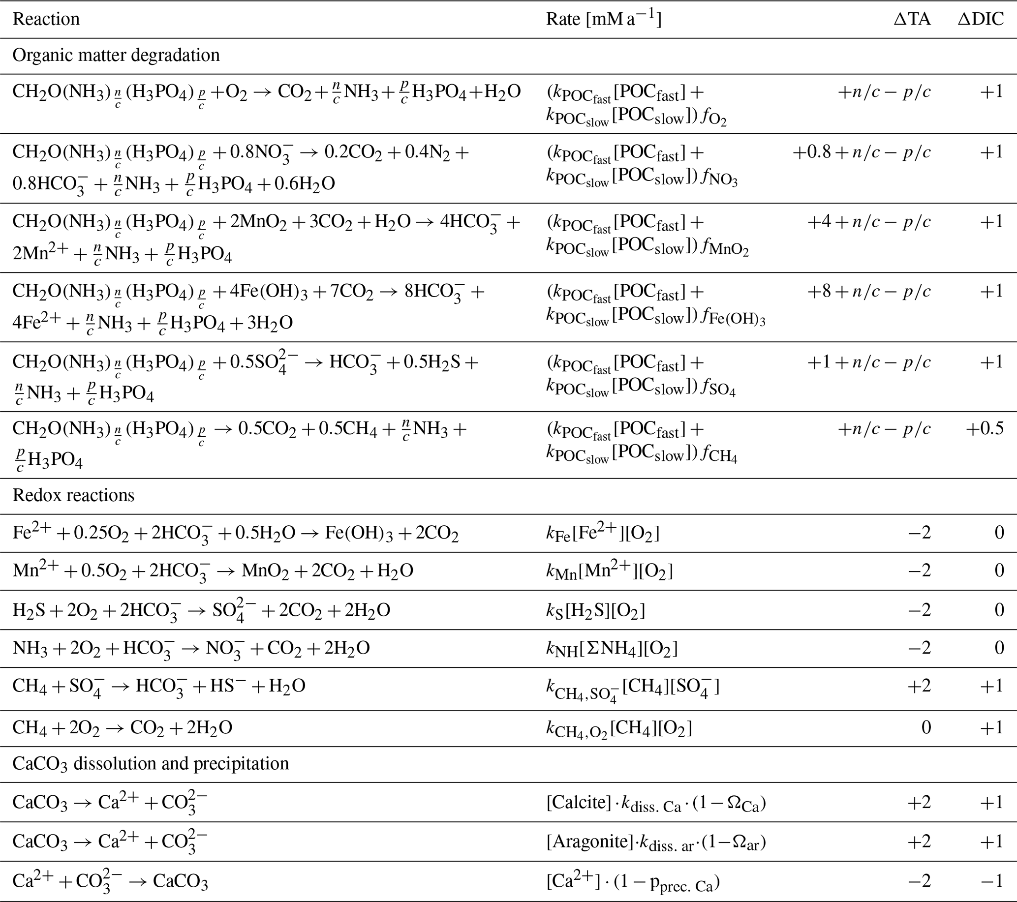
Table 1 summarizes the reactions, reaction rates, and stoichiometric relationships implemented in RADIv2, adapted from Sulpis et al. (2022) and Boudreau (1996). A more detailed description of the processes and parameters is available in Sulpis et al. (2022). The stoichiometric ratios $\frac{n}{c}$ and $\frac{p}{c}$ represent the nitrogen-to-carbon and phosphorus-to-carbon ratios in organic matter, respectively. By default, the model applies a Redfield ratio of $\mathrm{106}:\mathrm{16}:\mathrm{1}$ (Redfield, 1934), but these values can be adjusted to location-specific conditions or organic matter input sources. The degradation rate constants $k_{{\text{POC}}_{\text{fast}}}$ and $k_{{\text{POC}}_{\text{slow}}}$ describe the breakdown of fast- and slow-degrading organic matter. These rate constants are not fixed globally; they exhibit variability depending on the source and composition of organic matter and they are typically adjusted to represent the specific conditions of each modeled environment (Arndt et al., 2013; Kuderer and Middelburg, 2024). The rate constants for the fast and slow organic carbon pools can be specified directly by the user, for example based on literature values or in-situ measurements, or they can be diagnosed from the empirical flux relationship used in RADIv1 (tuned for deep-sea settings (Sulpis et al., 2022)). A refractory organic carbon pool is also included in the model structure, but its reactivity is set to zero by default, so it does not remineralize. The refractory fraction can be prescribed as a user-defined fraction of the incoming POM rain, in which case it affects sediment burial rates (computed from the total particulate rain to the sediments) and the bulk carbon content of the sediment column.

The rate constants for the redox reactions in RADIv2 are uniform globally and are described in Sulpis et al. (2022) and the references therein. The dissolution rate constants for calcite and aragonite (k_{diss. Ca} and k_{diss. ar}) control the dissolution dynamics of these carbonates, while the precipitation rate constant for calcite regulates the rate of calcite (p_{prec. Ca}) formation through precipitation. RADIv2 uses the same carbonate dissolution–precipitation scheme as RADIv1, non-linear kinetics for both calcite and aragonite dissolution described by Naviaux et al. (2019) and Dong et al. (2019). The terms $f_{{\mathrm{O}}_{\mathrm{2}}},f_{{\mathrm{NO}}_{\mathrm{3}}},f_{{\text{MnO}}_{\mathrm{2}}},f_{{\text{Fe(OH)}}_{\mathrm{3}}},f_{{\text{SO}}_{\mathrm{4}}},f_{{\text{CH}}_{\mathrm{4}}}$, represent the fractions of organic carbon degraded by each respective available oxidant. Oxidant limitation and interactions between pathways are modeled using widely applied Michaelis–Menten-type functions, which account for the influence of oxidant availability and the potential for certain oxidants to inhibit alternative metabolic pathways (Froelich et al., 1979; Boudreau, 1996; Soetaert et al., 1996a). This approach ensures that the model captures the overlapping and dynamic nature of these processes across the sediment depth. ΔTA quantifies the net change in total alkalinity associated with each reaction. ΣCO₂ represents the sum of dissolved inorganic carbon produced or consumed during the reactions.

It is important to note that the reactions presented in Table 1 reflect how they are handled within RADIv2, rather than their canonical representations. RADIv2 does not explicitly solve for H⁺ concentrations; instead, the model tracks DIC and TA, indirectly approximating the proton balance. The proton balance is estimated using a single Newton-Raphson iteration (Humphreys et al., 2022a; Sulpis et al., 2022). Consequently, reactions are expressed in terms of CO₂ and HCO${}_{\mathrm{3}}^{-}$ to align with model handling of DIC and TA, even though these species may not appear in the canonical representations of the reactions.

Table 1 Summary of reactions, reaction rates, and stoichiometric relationships implemented in RADIv2. The table includes degradation rates for organic matter, dissolution and precipitation rate constants for carbonates, and the fractions of organic carbon degraded by different oxidants, along with their impact on alkalinity and dissolved inorganic carbon concentrations.

2.1.2 Method of lines and transport mechanisms

At present time, DifferentialEquations.jl only solves Ordinary Differential Equations (ODEs); however, the fundamental transport equations (Eqs. 1 and 2) are partial differential equations (PDEs) in both time (∂t) and depth (∂z). The Method of Lines (MOL) numerical technique was employed to transform the transport PDEs into a system of ODEs compatible with DifferentialEquations.jl version v7.14.0. This is achieved by discretizing the spatial domain into finite depth intervals (dz), while keeping time (t) as a continuous variable. The sediment column is divided into these discrete depth intervals and the rate of change in solute concentrations over time is computed for each depth segment, following the approach described in Boudreau (1996).

To approximate the spatial derivatives of concentration profiles, a central difference approach is applied to the transport equations. This numerical method estimates spatial derivatives by evaluating concentration differences at two points on either side of a reference point (z), and assumes the concentration profile between points is approximately linear over small intervals of dz.

For a concentration profile (v, representing either a solute or solid concentration), the central difference approximation for second-order derivatives at point z is:

$$\begin{array}{}\text{(3)}& {\displaystyle \frac{{\partial }^{\mathrm{2}}v}{\partial z^{\mathrm{2}}}}\approx {\displaystyle \frac{v_{(z+\mathrm{d}z)}-\mathrm{2}{v}_z+v_{(z-\mathrm{d}z)}}{\mathrm{d}{z}^{\mathrm{2}}}}\end{array}$$

and a backward difference scheme for first-order derivatives:

$$\begin{array}{}\text{(4)}& {\displaystyle \frac{\partial v}{\partial z}}\approx {\displaystyle \frac{v_{(z+\mathrm{d}z)}-v_{(z-\mathrm{d}z)}}{\mathrm{2}\mathrm{d}z}}\end{array}$$

Using this central difference approach, (bio)diffusion is computed as follows:

$$\begin{array}{}\text{(5)}& \begin{array}{rl}{D}_z\left(v\right)& =d_{z,T}\left(v\right){\displaystyle \frac{{\mathit{\delta }}^{\mathrm{2}}v}{\mathit{\delta }{z}^{\mathrm{2}}}}\\ & =d_{z,T}\left(v\right)\cdot (v_{(z-\mathrm{d}z)}-\mathrm{2}{v}_z+v_{(z+\mathrm{d}z)})/\mathrm{d}{z}^{\mathrm{2}}\end{array}\end{array}$$

where v represents either C (solute concentration) or S (solid concentration). d_z,T(v) [m² a⁻¹] denotes the effective diffusion coefficient for solutes and the bioturbation mixing rate for solids (b_z). The bioturbation mixing rate (b_z) is empirically based on a 53-site data set compiled by Morford and Emerson (1999) ranging from the deep sea to the shelves (Archer et al., 2002).

$$\begin{array}{}\text{(6)}& b_z=b_{\mathrm{0}}{e}^{-(z/{\mathit{\lambda }}_{\mathrm{b}}{)}^{\mathrm{2}}}{\displaystyle \frac{[{\mathrm{O}}_{\mathrm{2}}{]}_{\mathrm{w}}}{[{\mathrm{O}}_{\mathrm{2}}{]}_{\mathrm{w}}+\mathrm{0.02}}},\end{array}$$

where b₀ is the surface bioturbation rate, calculated as $\mathrm{0.02328}\times {\mathrm{10}}^{-\mathrm{4}}\times (\mathrm{100}\times F_{\mathrm{POC}}{)}^{\mathrm{0.85}}$, following Archer et al. (2002), with F_POC being the incoming particulate organic carbon rain, converted from POM according to OM stoichiometry. The characteristic depth λ_b=0.08 m (Archer et al., 2002) and [O₂]_w [mol m⁻³] is the oxygen concentration of bottom waters.

Advection is calculated as:

$$\begin{array}{}\text{(7)}& \begin{array}{rl}& \text{advection}=-u{\displaystyle \frac{\mathit{\delta }v}{\mathit{\delta }z}}=\\ & \left\{\begin{array}{ll}\text{solute}& A_z\left(C\right)=-(u_z-\frac{d_{z,\mathrm{T}}\left(C\right)}{{\mathit{\phi }}_z}\cdot \frac{d{\mathit{\phi }}_z}{\mathrm{d}z}-d_{\mathrm{T}}^{\mathit{°}}(C)\\ & \cdot \frac{d(\mathrm{1}/{\mathit{\theta }}_z^{\mathrm{2}})}{\mathrm{d}z})\cdot \frac{C_{z+\mathrm{d}z}-C_{z-\mathrm{d}z}}{\mathrm{2}\mathrm{d}z}\\ \text{solid}& A_z\left(S\right)=-(w_z-\frac{d{b}_z}{\mathrm{d}z}-\frac{b_z}{{\mathit{\phi }}_{S,z}}\cdot \frac{d{\mathit{\phi }}_{s,z}}{\mathrm{d}z})\\ & \cdot \frac{(\mathrm{1}-{\mathit{\sigma }}_z)S_{z+\mathrm{d}z}+\mathrm{2}{\mathit{\sigma }}_z{S}_z-(\mathrm{1}+{\mathit{\sigma }}_z)S_{z-\mathrm{d}z}}{\mathrm{2}\mathrm{d}z},\end{array}\right.\end{array}\end{array}$$

The term u in $-u\frac{\mathit{\delta }v}{\mathit{\delta }z}$ represents the effective advection term, which is modified by additional corrections to account for changes in porosity, tortuosity, and bioturbation gradients. $d_{\mathrm{T}}^{\mathit{°}}\left(C\right)$ [m² a⁻¹] is the “free-solution” molecular diffusion coefficient for a solute and θ_z [–] is the depth-dependent tortuosity (${\mathit{\theta }}_z=\sqrt{\mathrm{1}-\mathrm{2}\text{ln}\left({\mathit{\phi }}_z\right)}$) (Boudreau, 1996), and σ_z [–] parameterizes influence of advection relative to bioturbation (Fiadeiro and Veronis, 1977; Boudreau, 1996). The parameter σ_z is introduced for the advective transport of solids because a more sophisticated numerical approach is needed when biodiffusion diminishes at depth within the sediment column. Under these conditions, the central difference scheme becomes unstable when applied to advective (burial) terms (Boudreau, 1996). A weighted difference scheme developed by Fiadeiro and Veronis (1977) is employed, that introduces the parameter σ_z (${\mathit{\sigma }}_z=\frac{\mathrm{1}}{\tanh \left(P{e}_z\right)}-\frac{\mathrm{1}}{P{e}_z}$), which represents half of the cell Peclet number ($P{e}_{\mathrm{h}}=\frac{w_z\cdot \mathrm{d}z}{\mathrm{2}{b}_z}$) and measures the relative influence of advection compared to biodiffusion over a given depth interval. When Pe_z≪1, biodiffusion dominates, whereas when Pe_z≫1, advection becomes the primary transport mechanism. The scheme transitions from a centered-difference approach under diffusion-dominant conditions to a backward-difference approach when advection dominates, and ensures numerical stability even as biodiffusion approaches zero (Fiadeiro and Veronis, 1977). This correction is not applied to solutes, where advection dominance is uncommon (Boudreau, 1996).

The mixing of solutes caused by burrow flushing or ventilation occurs through multiple processes that are collectively termed irrigation, which is computed as

$$\begin{array}{}\text{(8)}& I_{t,z}\left(C\right)={\mathit{\alpha }}_z(C_{\mathrm{w}}-C_z),\end{array}$$

where α_z is an irrigation coefficient, approximating an ensemble of biological processes, C_w is the solute concentration in the bottom waters and C_z is the concentration at depth z. Archer et al. (2002) derived α_z profile based on a 53-site dataset compiled by Morford and Emerson (1999), ranging from deep sea to shelves, expressing the irrigation coefficient as a function of the organic carbon deposition flux and the oxygen concentration of the overlaying water:

$$\begin{array}{}\text{(9)}& \begin{array}{rl}{\mathit{\alpha }}_{\mathrm{0}}& =\mathrm{11}\left({\displaystyle \frac{{\tan }^{-\mathrm{1}}\left(\frac{\mathrm{5}{F}_{\mathrm{POC}}\times {\mathrm{10}}^{\mathrm{2}}-\mathrm{400}}{\mathrm{400}}\right)}{\mathit{\pi }}}+\mathrm{0.5}\right)\\ & -\mathrm{0.9}+{\displaystyle \frac{\mathrm{20}[{\mathrm{O}}_{\mathrm{2}}{]}_{\mathrm{w}}}{[{\mathrm{O}}_{\mathrm{2}}{]}_{\mathrm{w}}+\mathrm{0.01}}}\cdot {\displaystyle \frac{F_{\mathrm{POC}}\times {\mathrm{10}}^{\mathrm{2}}}{F_{\mathrm{POC}}\times {\mathrm{10}}^{\mathrm{2}}+\mathrm{30}}}\cdot e^{\frac{-[{\mathrm{O}}_{\mathrm{2}}{]}_{\mathrm{w}}}{\mathrm{0.01}}}.\end{array}\end{array}$$

The per-depth irrigation coefficient follows:

$$\begin{array}{}\text{(10)}& {\mathit{\alpha }}_z={\mathit{\alpha }}_{\mathrm{0}}{e}^{-(z/{\mathit{\lambda }}_i{)}^{\mathrm{2}}},\end{array}$$

where the characteristic depth λ_i is 5 cm (Archer et al., 2002).

The contribution of biogeochemical reactions (∑R) are summarized in Table 1.

At the sediment–water interface, RADIv2 allows for prescribed solid fluxes and regulates solute exchange through a diffusive boundary layer. Following Boudreau (1996), advection and diffusion at z=0 for both solutes and solids are calculated as follows:

$$\begin{array}{}\text{(11)}& C_{-\mathrm{d}z}=C_{\mathrm{d}z}+{\displaystyle \frac{\mathrm{2}{\mathit{\theta }}_z^{\mathrm{2}}\mathrm{d}z}{\mathit{\delta }}}(C_{\mathrm{w}}-C_{\mathrm{0}})\end{array}$$

and

$$\begin{array}{}\text{(12)}& S_{-\mathrm{d}z}=S_{\mathrm{d}z}+{\displaystyle \frac{\mathrm{2}\mathrm{d}z}{b_{\mathrm{0}}}}\left({\displaystyle \frac{F_{\mathrm{s}}}{{\mathit{\phi }}_{s,\mathrm{0}}}}-w_{\mathrm{0}}{S}_{\mathrm{0}}\right)\end{array}$$

respectively. Here, C_−dz and S_−dz are imaginary concentrations used to solve transport across the SWI. For solutes, δ denotes the thickness of the DBL [m], C_w is the solute concentration in the well-mixed overlaying waters [mol m⁻³], and C₀ is the solute concentration at the SWI [mol m⁻³]. For solids, F_s is the particulate deposition flux at the SWI [mol m² a⁻¹], w₀ is the solid burial velocity at the SWI [a⁻¹], and S₀ is the particulate concentration at the SWI [mol m⁻³].

The bottom boundary condition is characterized by a “no-gradient” constraint, meaning that the concentration remains constant at the boundary:

$$\begin{array}{}\text{(13)}& v_{Z+\mathrm{d}z}=v_{Z-\mathrm{d}z},\end{array}$$

where v stands for either C (solute concentration) or S (solid concentration), Z is the boundary of the modeled sediment domain, v_Z+dz is the concentration outside of the sediment domain, and v_Z−dz is the deepest depth interval within the modeled sediment domain.

2.2 Additions to RADIv2

RADIv1 was designed for deep-sea sediments and does not account for methane or solute transport by bottom-water hydrodynamics (Sulpis et al., 2022). In RADIv2, we added methane to address its role in sediment biogeochemistry, particularly in coastal regions where methane formation and release can play a larger role compared to the deep sea. In coastal and shelf environments, hydrodynamic properties are highly variable and can influence key transport mechanisms, such as the thickness of the DBL (Levich and Tobias, 1963; Santschi et al., 1983; Lorke et al., 2003) and enhanced porewater diffusivity through dispersion (McGinnis et al., 2014).

2.2.1 Diffusive boundary layer thickness

In RADIv1, the DBL thickness was prescribed as a fixed value. However, in reality, it varies with bottom-water hydrodynamics and differs by solute due to their distinct molecular diffusion rates (Levich and Tobias, 1963; Yuan-Hui and Gregory, 1974; Santschi et al., 1983; Lorke et al., 2003). The DBL thickness is primarily controlled by bottom-water currents, ranging from tens of microns in high-energy environments (e.g., coastal areas and rivers) to several millimeters in the low-energy deep sea (Sulpis et al., 2019). The benthic O₂ uptake of coastal sediments can fluctuate by more than 30 % within hours or days, driven by variations in the thickness of the DBL (Glud et al., 2007). To account for this, a hydrodynamic- and solute-dependent DBL thickness is implemented in RADIv2, following the combined approach of Sulpis et al. (2018) and Lorke and Peeters (2006). The vertical velocity profile of bottom-water currents is approximated using the Law of the Wall (LOW) equation used in Sulpis et al. (2018):

$$\begin{array}{}\text{(14)}& U={\displaystyle \frac{u^{*}}{\mathit{\kappa }}}\ln \left({\displaystyle \frac{\mathit{\kappa }{u}^{*}}{f\mathit{\nu }}}\right)+C{u}^{*},\end{array}$$

where U is the bottom-water current velocity [m s⁻¹], κ is the von Karman constant (0.40) [unitless], u^* is the friction velocity [m s⁻¹], ν is the kinematic viscosity of seawater [${\mathrm{10}}^{-\mathrm{2}}{\text{cm}}^{\mathrm{2}}{\text{s}}^{-\mathrm{1}}$] and C is an empirical dimensionless constant with a value of 5.1 (Monin and Yaglom, 1971). The Coriolis parameter f was approximated as $\mathrm{1}\times {\mathrm{10}}^{-\mathrm{4}}$ [s⁻¹], a value representative of mid-latitudes. However, f is latitude-dependent, varying as f=2Ωsin ϕ where ϕ is the latitude and $\mathrm{\Omega }=\mathrm{7.2921}\times {\mathrm{10}}^{-\mathrm{5}}$ rad s⁻¹ is the Earth's angular velocity. It is zero at the equator (ϕ=0°) and reaches a maximum of $\mathrm{1.45}\times {\mathrm{10}}^{-\mathrm{4}}$ s⁻¹ at the poles ((ϕ=90°)). To assess the sensitivity of bottom-water current velocity to variations in f, we recalculated U for latitudes ranging from 1 to 90°, keeping the kinematic viscosity of seawater (ν) constant at 10⁻⁶ m² s⁻¹ and u^* at 0.1 m s⁻¹. The resulting U values were 6.38 m s⁻¹ (1°), 5.54 m s⁻¹ (30°), 5.40 m s⁻¹ (60°), and 5.37 m s⁻¹ (90°). These results show that U stabilizes at higher latitudes but increases significantly near the equator due to the near-zero Coriolis parameter. Future work could improve this parameterization by explicitly incorporating latitude dependence (ϕ), enhancing the model’s applicability across diverse geographic regions.

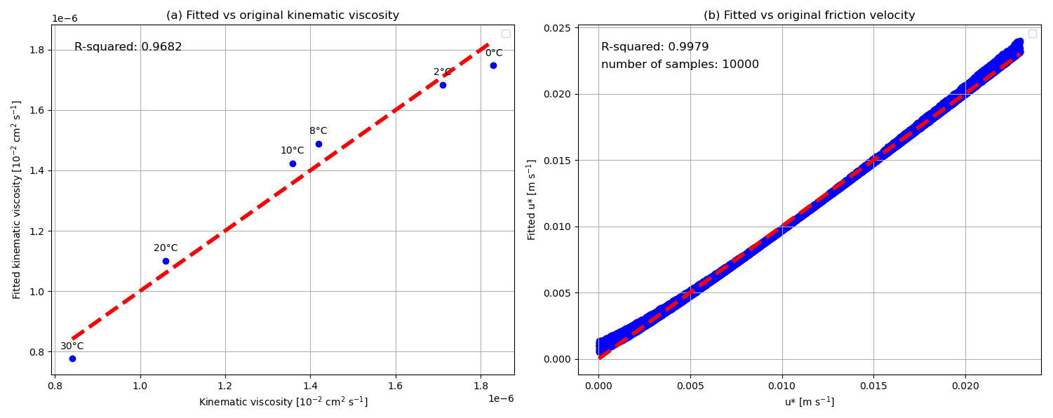
Figure 1a presents the empirical relationship between the kinematic viscosity of seawater (ν) and bottom-water temperature (T, in °C), derived by fitting data from ITTC (2011). The resulting linear equation is:

$$\begin{array}{}\text{(15)}& \mathit{\nu }=\mathrm{1.75}\times {\mathrm{10}}^{-\mathrm{6}}-\mathrm{3.24}\times {\mathrm{10}}^{-\mathrm{8}}\times T.\end{array}$$

By substituting this empirical relation for (ν) (Eq. 15) into Eq. (14), we obtain an equation linking bottom current speeds (U), bottom-water temperature (T), and friction velocity (u^*). This relationship, for T=0 to 40 °C and U up to 1.1 m s⁻¹, is depicted in Fig. 1b and is expressed in Eq. (14) as

$$\begin{array}{}\text{(16)}& \begin{array}{rl}{u}^{*}& =\mathrm{0.00136}-\mathrm{2.19598542}\times {\mathrm{10}}^{-\mathrm{5}}\\ & \times T+\mathrm{2.35862843}\times {\mathrm{10}}^{-\mathrm{2}}\times U.\end{array}\end{array}$$

The mass transfer coefficient as a function of u^* is approximated following Lorke and Peeters (2006):

$$\begin{array}{}\text{(17)}& k={\displaystyle \frac{\mathrm{1}}{\mathrm{9}}}S{c}^{-\mathrm{1}/\mathrm{2}}{u}^{*},\end{array}$$

where k is the mass transfer coefficient [m a⁻¹] and Sc is the dimensionless Schmidt coefficient, defined as $Sc=\mathit{\nu }/d^{\mathit{°}}\left(v\right)$, in which d^°(v,T) [m² s⁻¹] is the temperature-dependent molecular diffusion coefficient of the solute.

The DBL thickness (δ_DBL) [m] is obtained by dividing molecular diffusion coefficient ($d_{v,\mathrm{T}}^{\mathit{°}}$) by the the mass transfer coefficient (k), following Sulpis et al. (2018) as

$$\begin{array}{}\text{(18)}& {\mathit{\delta }}_{\mathrm{DBL}}={\displaystyle \frac{d_{v,T}^{\mathit{°}}}{k}}.\end{array}$$

Figure 1 (a) Empirical relationship between kinematic viscosity (ν) and bottom-water temperature (T), fitted to the original data (ITTC, 2011). (b) Fitted friction velocity (u^*) as a function of bottom-water temperature (T) and bottom-current speed (U) compared to the original u^* values.

2.2.2 Pore water dispersion

In permeable sediments (permeability $>{\mathrm{10}}^{-\mathrm{12}}$ m² (Huettel et al., 2014)), enhanced pore water diffusivity, or dispersion, is driven by flow interaction with bottom water topography, density and pressure gradients, and migrating sediment ripples and wave motion (Boudreau, 1997; Huettel et al., 2014). The net effect on vertical transport can be represented as enhanced pore water diffusivity (Boudreau, 1997), which is estimated as a function of shear velocity (u^*), following the relation described in McGinnis et al. (2014):

$$\begin{array}{}\text{(19)}& K_{v,z,\mathrm{T}}=d_{v,z,\mathrm{T}}{e}^{\mathit{\alpha }\mathit{\kappa }{u}^{*}},\end{array}$$

where $K_{v,z,\mathrm{T}}$ is the apparent bulk sediment diffusivity (dispersion) [m² s⁻¹], $d_{v,z,\mathrm{T}}$ is the effective diffusion coefficient, corrected for sediment tortuosity [m² s⁻¹], α is a sediment-permeability-dependent fit parameter [s m⁻¹] (set to 1, based on permeable sediments from the Wadden Sea and North Sea, following McGinnis et al., 2014), κ is the von Kármán constant [–], and u^* is the friction velocity [mm s⁻¹].

For sediments with permeability below 10⁻¹² m², dispersive transport is considered negligible (Huettel et al., 2014), and α is set to 0, such that, in the absence of advection, only molecular diffusion governs solute transport. For permeable sediments (> 10⁻¹² m²), sediment dispersion ($K_{v,z,\mathrm{T}}$) is incorporated as the effective diffusion coefficient ($d_{v,z,\mathrm{T}}$) in solute transport equations (Eqs. 3 and 5), accounting for both diffusion and advection.

2.2.3 Numerical methods and computational enhancements

The original RADIv1 framework used a forward Euler method to solve fundamental transport equations, which requires user-defined time and depth steps that must adhere to a specific ratio to ensure numerical stability (Sulpis et al., 2022). However, in coastal environments with steep solute gradients between porewater and bottom waters, as well as high microbial activity, this numerical scheme can become unstable and computationally inefficient. Capturing the complexity of sediment processes requires sufficient vertical discretization, which increases computational demand. RADIv1 and RADIv2 are the first diagenetic models built using DifferentialEquations.jl, a high-performance and modular Julia package for solving differential equations (Rackauckas and Nie, 2017). Coastal sediments may require higher-order stiff solvers with fine-tuned tolerance settings to ensure numerical stability while maintaining computational efficiency. In contrast, deep-sea environments, where geochemical processes evolve over longer timescales with more gradual changes, can be simulated using computationally-efficient solvers that prioritize stability over high temporal resolution. RADIv2 allows users to configure solver options, including time-stepping strategies, stiffness detection, and convergence criteria, based on the specific characteristics of the sediment environment being simulated. Additionally, DifferentialEquations.jl integrates with Julia’s multi-threading and multiprocessing capabilities, allowing RADIv2 to handle computationally-intensive tasks, such as ensemble simulations, with reduced runtime. Users can define the number of trajectories and specify parameters for each trajectory individually, either by explicitly setting values or randomizing them within predefined ranges. This ensemble approach enables a more-comprehensive exploration of model behavior, particularly in cases where input parameters are uncertain or highly variable. Instead of relying on single-point estimates, users can systematically vary key input parameters such as organic matter flux, bottom-water temperature, and calcite saturation state within defined ranges. This flexibility is especially useful in coastal environments, where such parameters exhibit significant spatial and temporal variability. Additionally, this capability can be used to constrain unknown parameters by comparing simulation results with observational data. The resulting model outputs form an envelope of potential outcomes that aligns well with in situ data, which is also typically reported as ranges due to variability within measurement periods.

Building upon an open-source programming language, RADIv2 leverages Julia’s flexibility to integrate external packages, including optimization frameworks. One such package, BlackBoxOptim.jl (Feldt and Stukalov, 2018), provides an efficient, derivative-free approach to parameter tuning. This heuristic optimization algorithm employs an adaptive gradient strategy, beginning with broader exploratory steps before refining its search space for improved convergence. This adaptability ensures optimization across a wide range of environmental conditions while minimizing the risk of becoming trapped in local minima. By incorporating BlackBoxOptim.jl, RADIv2 allows users to fine-tune model parameters to align with observational data. This feature is particularly useful for constraining the best fit to observations for highly variable or unknown model parameters. RADIv2 includes an example script demonstrating how to optimize key parameters (https://doi.org/10.5281/zenodo.18386461, van der Zant et al., 2025). This script serves as a practical guide, showcasing how users can refine model outputs to match empirical data. Furthermore, this optimization framework can be extended beyond the examples provided, allowing users to fine-tune any model parameter to improve representation across different marine environments.

2.2.4 Performance of RADIv2 versus RADIv1

Here we present a quantitative benchmark comparison of RADIv2 versus RADIv1. To keep the comparison as direct as possible, we re-ran the deep-sea Southern Pacific case (input file IC_SM7) from the original RADIv1 paper with both model versions, using comparable physics (no dispersion, constant DBL, identical forcing and boundary conditions). All timings reported below are for a single CPU core.

For a 50-year spin-up, RADIv1 required 5 min and 20 s, whereas RADIv2 (using the Rosenbrock23 stiff solver with a sparse KLU linear solver, abstol $=\mathrm{1}\times {\mathrm{10}}^{-\mathrm{6}}$ and reltol $=\mathrm{5}\times {\mathrm{10}}^{-\mathrm{3}}$) completed in 40 s.

For a 2000-year integration of the same set-up, RADIv1 required ≈4 hours and 30 min, while RADIv2 completed in ≈ 27 min.

When the additional physics implemented in RADIv2 are activated (species- and U-dependent DBL thickness and dispersion) for the same 2000-year run, the wall-clock time remains of the same order, at 28 min and 30 s. Thus, the added physical realism does not make the system substantially more expensive.

The main performance gain comes from the stiff ODE integrator (Rosenbrock23) with adaptive time-stepping combined with a sparse linear solver (KLU). RADIv1 uses a forward Euler scheme with a constant time step, forcing the model to continue using this small step even after the solution is close to steady state. RADIv2's adaptive time-stepping takes many small steps initially, then increases the time step once the system has largely equilibrated. Moreover, using a sparse factorization like KLU stores and operates only on the non-zero entries of the Jacobian, which reduces both memory use and computation, so stiff simulations can run faster.

The DifferentialEquations.jl solve function scales the local error estimate as

$${\mathrm{err}}_{\mathrm{scaled}}={\displaystyle \frac{\mathrm{err}}{\text{abstol}+\text{reltol}\times max\left(u_{\mathrm{prev}},u\right)}}$$

where u_prev and u are the solution values before and after the step (Rackauckas and Nie, 2017). For typical state-variable magnitudes in this study (roughly mmol m⁻³ to mol m⁻³), the relative term dominates and the local error scale is approximately reltol×u, while abstol provides a hard absolute scale for very small concentrations. For example, for u=1 mol m⁻³ the scale is ${\mathrm{10}}^{-\mathrm{6}}+\mathrm{5}\times {\mathrm{10}}^{-\mathrm{3}}\times \mathrm{1}=\mathrm{5.001}\times {\mathrm{10}}^{-\mathrm{3}}$ mol m⁻³ (about 0.5 % of u), and for u=1 mmol m${}^{-\mathrm{3}}={\mathrm{10}}^{-\mathrm{3}}$ mol m⁻³ it is ${\mathrm{10}}^{-\mathrm{6}}+\mathrm{5}\times {\mathrm{10}}^{-\mathrm{3}}\times {\mathrm{10}}^{-\mathrm{3}}=\mathrm{6}\times {\mathrm{10}}^{-\mathrm{6}}$ mol m⁻³ (0.6 % of u). When concentrations are very small, the absolute term prevents the tolerated error scale from dropping below 10⁻⁶. We consider this sub-percent tolerance scale for typical concentrations acceptable for equilibrium benthic fluxes, as uncertainties in boundary conditions, parameter values, and process representations tend to be larger than the error of the solver.

2.2.5 Methane

In RADIv1, methane, a potent greenhouse gas, was not included as a modeled solute due to its limited role in deep-sea sediments. Methane is produced in anoxic sediment layers through methanogenesis, a fermentation process that occurs once electron acceptors – such as oxygen, nitrate, and sulfate – are depleted. This pathway is primarily relevant in coastal and continental shelf sediments, where high organic matter flux supports rapid sulfate consumption and creates conditions favorable to methane production. In contrast, deep-sea sediments rarely reach the methanogenic zone due to lower organic matter fluxes and sufficient availability of favorable electron acceptors. Once formed, methane is largely consumed within the sediment by microbial oxidation before reaching the overlying water column. The primary sink for methane is anaerobic oxidation, facilitated by sulfate-reducing bacteria (Hinrichs et al., 1999; Egger et al., 2018). Aerobic oxidation can also occur near the sediment-water interface where oxygen is present, though it is typically a less significant pathway. Approximately 80 % of methane oxidation occurs in continental shelf sediments (Egger et al., 2018). However, recent studies suggest that anaerobic oxidation of methane does not become substantially more efficient with warming, whereas warming can enhance methane production within the sediments (Stranne et al., 2022). As a result, a larger fraction of climate-driven seafloor methane production may bypass the sedimentary filter and reach the water column. The inclusion of methane in RADIv2 enables explicit simulation of methane production and oxidation pathways, providing a framework to assess how changing environmental conditions may influence benthic methane cycling and seafloor seepage.

3 Model validation

Benthic-pelagic coupling plays a fundamental role in ocean biogeochemistry, influencing carbon sequestration, nutrient cycling, and climate regulation (Soetaert et al., 2000). To assess how well RADIv2 represents this coupling, we apply the model to six marine environments: the North Sea, Monterey Bay, the shallow Iberian margin, the deep Iberian margin, and two deep-sea stations in the Arabian Sea. These sites span a range of sedimentary and hydrodynamic conditions, from productive coastal systems to deep-sea settings. Because observations and simulations are not always fully paired in space or forcing (not all parameters or boundary conditions are available to constrain RADIv2) and sample sizes differ, we use a Welch two-sample t-test (Welch, 1938) to evaluate whether the mean modelled flux differs significantly from the mean of the observations. To account for the strong spatial heterogeneity of benthic fluxes, we also quantify the fraction of simulated values that fall within the “bulk” observational interquartile range (25 %–75 %) and within the broader 5 %–95 % observational envelope. Together, these diagnostics provide a joint measure of systematic bias (over- or underestimation) and of how well the modelled fluxes remain within the range documented in the literature.

The benthic flux (J_v) of a given solute across the SWI is driven by the concentration gradient across the DBL and follows the formulation of Sulpis et al. (2022):

$$\begin{array}{}\text{(20)}& J_v={\mathit{\phi }}_{\mathrm{0}}{d}_{v,\mathrm{T}}\times {\displaystyle \frac{v_{\mathrm{0}}-v_{\mathrm{w}}}{\mathit{\delta }}},\end{array}$$

where J_v [mol m⁻² a⁻¹] is the benthic solute flux, φ₀ [m³ m⁻³] is the porosity at the SWI, d_v,T [m² a⁻¹] is the effective diffusion coefficient, v₀ [mol m⁻³] and v_w [mol m⁻³] are solute concentrations at the SWI and in the bottom waters, respectively, and δ [m] is the thickness of the DBL.

To account for environmental variability, we performed ensemble simulations with RADIv2 in which five key parameters are varied: bottom-water temperature, current velocity, calcium saturation state, and the fluxes of particulate organic and inorganic carbon to the seafloor. For each site, the calcium carbonate state is computed from total alkalinity and dissolved inorganic carbon using the CO2SYS carbonate-chemistry routine (Lewis and Wallace, 1998; Humphreys et al., 2022a), which solves the carbonate system with standard equilibrium constants and calcite/aragonite solubility products following Mucci (1983) and applies pressure corrections following Ingle et al. (1973). The CO2System.jl module is available on https://doi.org/10.5281/zenodo.6395674 (Humphreys et al., 2022b).

These factors were selected because they are fundamental drivers of benthic hydrodynamics, organic matter degradation, and calcite dissolution. The same ensemble of RADIv2 fluxes forms the basis for the metamodel introduced in the next section. In addition, we illustrate the performance of RADIv2 for resolving depth profiles of porewater composition at a coastal margin station on the Iberian Margin (Sect. S1, Fig. S1 in the Supplement).

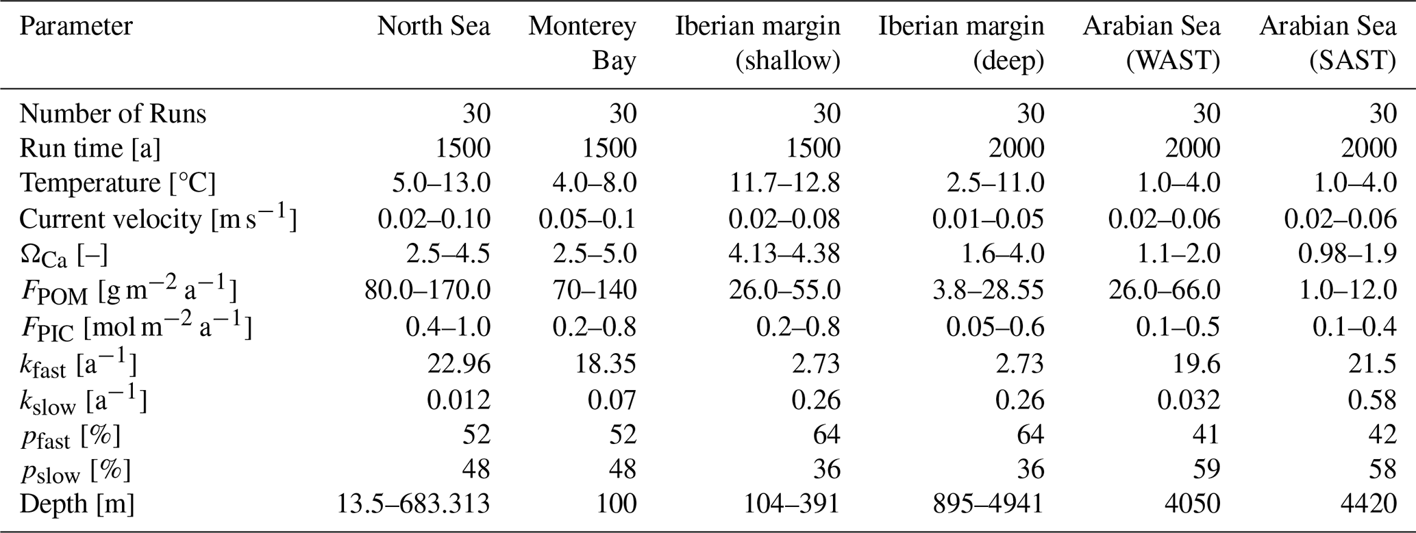
Table 2 summarizes the key model parameters used in the ensemble runs. All run files and input files are publicly available at https://doi.org/10.5281/zenodo.18386461 (van der Zant et al., 2025). Ensemble simulations were integrated with the stiff Rosenbrock23 solver to steady state, using adaptive time stepping and a sparse linear solver. Dissolved species equilibrate on time scales of years to decades, whereas particulate organic matter adjusts more slowly as it is buried. We therefore defined steady state by requiring that the maximum change in depth-integrated solid organic carbon (fast + slow pools) over the final 5 years of integration was less than 10⁻³ mmol m⁻³ across the full depth of the sediment column. Although all calibration experiments in this study are run to steady state, RADIv2 also supports transient simulations with time-dependent boundary conditions and forcings. A dedicated example with tidal current variability and seasonal plankton-bloom forcing is presented in the Sect. S2 in the Supplement. In all configurations used in this study, we employ a uniform vertical grid with a spacing of $\mathrm{d}z=\mathrm{5}\times {\mathrm{10}}^{-\mathrm{3}}$ m. A sensitivity test for different dz values for the Iberian Margin coastal is presented in Sect. S1 in the Supplement.

Table 2 Model parameters for the six marine environments. The five varying parameters are bottom-water temperature, current speed, bottom-water calcite saturation state (Ω_Ca), particulate organic matter flux (F_POM), and calcite flux (F_Ca). The parameters (k_fast, k_slow) represent the degradation rate constants for fast- and slow-degrading organic matter, respectively, while (p_fast, p_slow) denote the corresponding fractions of each organic matter type. Ω_Ca is calculated from environmental parameters using CO2SYS (Humphreys et al., 2022a).

3.1 North Sea

Figure 2a shows the fluxes simulated by RADIv2 alongside a comparison with values reported in the literature. For North Sea O₂ fluxes, the model shows a positive bias (mean 13.8 vs 10.9 mmol m⁻² d⁻¹; Welch p=0.003): one third of the simulated values fall within the observational 25 %–75 % range, while all lie within the 5 %–95 % observational envelope. For DIC, the model substantially overestimates the observed fluxes (mean 16.8 vs 8.9 mmol m⁻² d⁻¹; Welch $p=\mathrm{1.33}\times {\mathrm{10}}^{-\mathrm{7}}$), with ∼ 3  % of simulated values within the observational 25 %–75 % range and ∼ 23 % within the 5 %–95 % range, indicating that most model values exceed the bulk of observed variability. For North Sea TA fluxes, modelled and observed values overlap: all simulated fluxes fall within both the observational 25 %–75 % and 5 %–95 % ranges, and the Welch test (p=0.22) does not indicate a significant systematic bias, suggesting no model offset for TA.

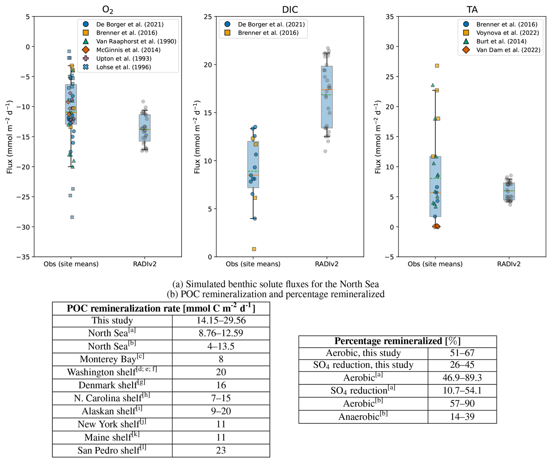
Figure 2 Comparison of simulated benthic solute fluxes and POC remineralization rates with values reported in the literature. (a) Simulated RADIv2 benthic solute fluxes for the North Sea compared to published values. Box–whisker plots compare the distribution of RADIv2 fluxes (“RADIv2”) with observational and modelled site means (“Obs”) (De Borger et al., 2021; Brenner et al., 2016; Van Raaphorst et al., 1990; McGinnis et al., 2014; Upton et al., 1993; Lohse et al., 1996; Voynova et al., 2019; Burt et al., 2014; Van Dam et al., 2022). The box spans the interquartile range (25 %–75 %), and the whiskers extend to the 5 %–95 % range. The solid orange horizontal line indicates the median, the green dashed line indicates the mean, and coloured jittered dots show individual observations. Negative O₂ fluxes correspond to uptake of oxygen by the sediment. (b) POC remineralization rates and percentage of remineralization in different shelf environments. ^a Upton et al. (1993); ^b De Borger et al. (2021); ^c Berelson et al. (2003); ^d Archer and Devol (1992); ^e Christensen et al. (1984); ^f Christensen et al. (1987); ^g Canfield et al. (1993); ^h Anderson et al. (1994); ⁱ Grebmeier and McRoy (1989); ^j Rowe et al. (1988); ^k Christensen (1989); ^l Berelson et al. (2002);

The simulated DIC fluxes for the North Sea are higher than the literature range. This likely reflects a combination of too strong organic-matter supply and too reactive organic-matter parameters in our set-up. The imposed POM rain is based on annual-mean export estimates, which smooth over episodic blooms and short-lived pulses and can therefore misrepresent the supply at the time of the benthic flux measurements. Combined with highly reactive incoming OM, most degradation occurs near the sediment–water interface and drives larger DIC fluxes (and slightly elevated O₂ uptake) than those inferred from the local measurements and modelling studies. Moreover, the model produces narrower flux ranges compared to in-situ measurements. This discrepancy can be attributed to the steady-state nature of the simulations, which do not account for transient variations such as temperature, tidal oscillations and internal waves. Internal waves, including their breaking counterparts, can induce sediment resuspension (Stastna and Lamb, 2008; Hosegood and van Haren, 2004), which in turn affects benthic fluxes (Niemistö and Lund-Hansen, 2019) and influences the benthic boundary layer through turbulence (Diamessis and Redekopp, 2006). Tidal cycles can also introduce substantial short-term variability in fluxes (McGinnis et al., 2014; Glud et al., 2007). These dynamic processes, which are not captured by steady-state simulations, can lead to significant fluctuations in solute and particulate fluxes across the sediment-water interface, particularly in coastal regions where wave action and tidal forcing are more pronounced.

The modeled remineralization rates (Fig. 2b) are within the same order of magnitude than those observed in continental shelf environments, although they exceed observations from the North Sea. This positive bias is consistent with the combination of relatively high imposed organic-matter supply and reactive organic-matter parameters discussed above. The relative contributions of aerobic and anaerobic remineralization in RADIv2 align with both reported values for North Sea sediments and typical continental shelf environments (Jørgensen, 1982) (Fig. 2b). This agreement indicates that RADIv2 captures organic matter degradation pathways under varying redox conditions.

3.2 Monterey Bay

For Monterey Bay (Fig. 3a), O₂ fluxes show good agreement between model and observations: the means are nearly identical (9.29 vs 9.11 mmol m⁻² d⁻¹), and no significant mean bias is detected (Welch p=0.85). Nearly all simulated values (97 %) fall within the observational 25 %–75 % range, and all lie within the 5 %–95 % envelope. For DIC, the predicts higher fluxes (mean 12.0 vs 9.95 mmol m⁻² d⁻¹), while the Welch test provides only marginal evidence for a mean difference (p=0.10), reflecting the small sample size (n_obs=7). About one third of simulated DIC values fall within the observational 25 %–75 % range and ∼ 87 % within the 5 %–95 % envelope. TA fluxes agree closely (means 4.46 vs 4.35 mmol m⁻² d⁻¹; Welch p=0.90), with 63 % of model values inside the observational 25 %–75 % range and all within the 5 %–95 % envelope.

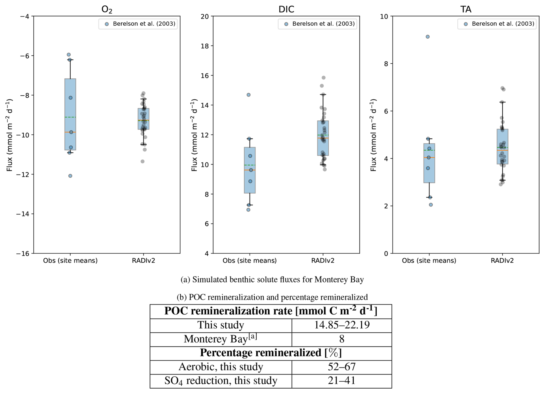
Figure 3 Comparison of simulated benthic solute fluxes and POC remineralization rates with values reported in the literature. (a) Simulated RADIv2 benthic solute fluxes for Monterey Bay compared to published values. Box–whisker plots compare the distribution of RADIv2 fluxes (“RADIv2”) with observational and modelled site means (“Obs”). The box spans the interquartile range (25 %–75 %), and the whiskers extend to the 5 %–95 % range. The solid orange horizontal line indicates the median, the green dashed line indicates the mean, and coloured jittered dots show individual observations. Negative O₂ fluxes correspond to uptake of oxygen by the sediment. (b) POC remineralization rates and percentage remineralized values for this study compared to Monterey Bay in-situ data Berelson et al. (2003). ^a Berelson et al. (2003).

The modest DIC bias likely reflects uncertainties in the imposed organic-matter supply and reactivity, while the comparatively narrow model spread in O₂ is consistent with the steady-state nature of the simulations, which do not resolve short-term variability. Internal tides and associated internal-wave activity have been shown to significantly influence sediment dynamics in Monterey Bay (Cheriton et al., 2014), but are not represented in the present set-up. RADIv2 simulates an organic matter remineralization rate for Monterey Bay that is approximately 2–3 times higher than observed rates (Fig. 3b). However, the values in Berelson et al. (2003) are lower than the global-mean C_org remineralization rate for continental shelf environments (∼ 12 mmol C m⁻² d⁻¹ (Berelson et al., 2003)). Because Berelson et al. (2003) did not measure POM rain to the seafloor directly, the POM flux range used in Table 2 was estimated by analogy with the North Sea calibration. This choice likely overestimates the actual organic-matter supply at Monterey Bay and contributes to the positive bias in the simulated remineralization rates. The relative contribution of aerobic and anaerobic organic matter pathways simulated by RADIv2 is consistent with values observed in other continental shelf studies (Fig. 3b) (Jørgensen, 1982).

3.3 Iberian Margin

The Iberian Margin validation uses data from five transects spanning a wide range of depths, as reported by Epping et al. (2002). Two input files were created: one for shallow locations (<400 m) and one for deeper locations (>400 m). For the simulations, the average organic carbon decay rate $k_{\mathrm{avg}}=p_f\times k_f+p_s\times k_{\mathrm{slow}}$ is constrained between 1.5 and 2.25 a⁻¹ (Table 2), based on high-resolution in-situ oxygen microprofiles (Epping et al., 2002).

For the Iberian Margin (Fig. 4a), RADIv2 overestimates O₂ uptake at both stations. At the shallow site, the mean simulated flux is 4.38 vs 2.75 mmol m⁻² d⁻¹, and at the deep site 2.38 vs 1.07 mmol m⁻² d⁻¹, with both Welch tests indicating a significant positive bias at each location ($p=\mathrm{1.45}\times {\mathrm{10}}^{-\mathrm{5}}$ and $p=\mathrm{2.47}\times {\mathrm{10}}^{-\mathrm{8}},$ respectively). At neither site do simulated values fall within the observational 25 %–75 % range, and ∼ 37 % (shallow) and ∼ 43 % (deep) lie within the 5 %–95 % observational envelope. The model also overestimates the C_org remineralization rates (Fig. 4b). Epping et al. (2002) already noted that the observed remineralization rates on the Iberian Margin are unexpectedly low given the high primary production in this region (∼ 7–11 mmol C m⁻² d⁻¹) and that they fall well below predicted values based on empirical relationships described in Middelburg et al. (1997). Shelf sediments off Peru exhibit rates of 5.3±2.9 mmol C m⁻² d⁻¹ (Fossing, 1990), and margin sediments off Chile, up to depths of 2000 m, show rates approximately 15 times higher (Thamdrup and Canfield, 1996). In our set-up, we adopt the export flux estimates from Epping et al. (2002) without additional site-specific tuning, so uncertainties in the effective POM supply at these stations likely contribute to the positive bias in RADIv2 remineralization rates. A dedicated comparison of simulated and observed O₂, NO${}_{\mathrm{3}}^{-}$ and NH${}_{\mathrm{4}}^{+}$ porewater profiles at station 99–6 is provided in Sect. S1 of the Supplement, where we also assess the sensitivity of these profiles and the associated fluxes to vertical resolution.

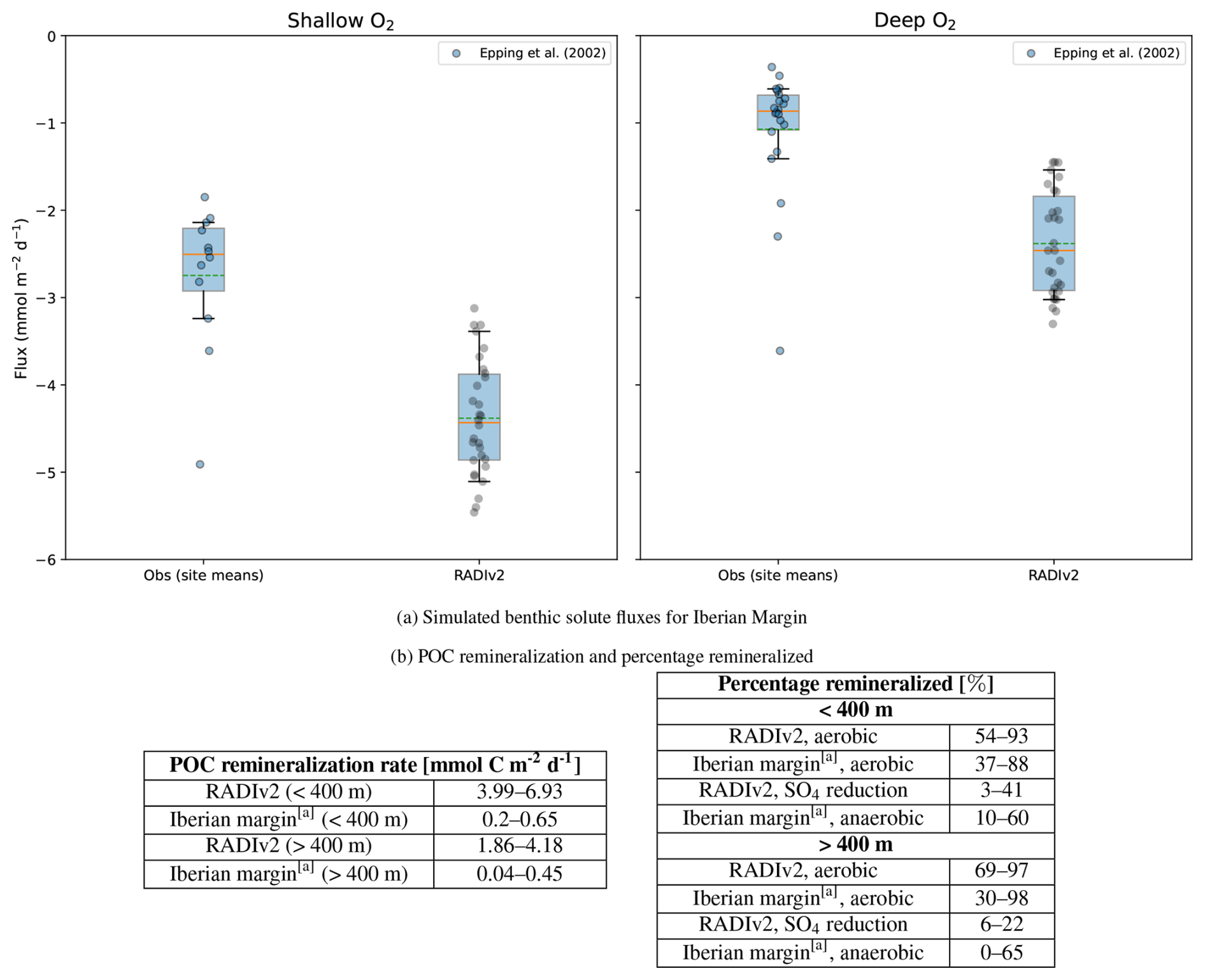
Figure 4 Comparison of simulated benthic solute fluxes and POC remineralization rates with values reported in the literature. (a) Simulated RADIv2 benthic solute fluxes for the Iberian Margin compared to published values. Box–whisker plots compare the distribution of RADIv2 fluxes (“RADIv2”) with observational and modelled site means (“Obs”). The box spans the interquartile range (25 %–75 %), and the whiskers extend to the 5 %–95 % range. The solid orange horizontal line indicates the median, the green dashed line indicates the mean, and coloured jittered dots show individual observations. Negative O₂ fluxes correspond to uptake of oxygen by the sediment. (b) POC remineralization rates and percentage remineralized values for this study compared to Epping et al. (2002). ^a Epping et al. (2002).

Although DIC fluxes were not directly measured in this study, they can be inferred from the modeled O₂ influx using the Respiratory Quotient (RQ), defined as the molar ratio of DIC production to O₂ consumption during organic matter remineralization (Jørgensen et al., 2022), RQ $=\frac{\mathrm{\Delta }\mathrm{DIC}}{\mathrm{\Delta }{\mathrm{O}}_{\mathrm{2}}}$. This approach provides a practical means of evaluating DIC fluxes in the absence of direct in-situ measurements. Under idealized conditions, where organic matter is represented by redfield organic matter, CH₂O, the RQ equals 1.0, reflecting a 1:1 stoichiometric ratio between O₂ consumption and DIC production. However, re-evaluated marine phytoplankton composition lead to slightly lower RQ values, around 0.88–0.90 (Hedges et al., 2002; Anderson, 1995). Some studies also account for additional oxygen-consuming processes, particularly nitrification, which further lowers RQ values (Tanioka and Matsumoto, 2020). Additional variability in RQ can come from incomplete reoxidation due to losses of N₂ or burial of FeS₂. FeS₂ can later be reoxidized through bioturbation-driven exposure to oxygen, further influencing oxygen demand and introducing additional variability in RQ in both directions. An empirical approach to deriving RQ values involves using in-situ measurements of benthic DIC efflux and O₂ influx. Flux-derived RQ values compiled by Jørgensen et al. (2022) span a broad range, from 0.69 to 1.31. The variation from theoretical stoichiometry can be attributed to factors including carbonate dissolution, which enhances DIC fluxes without directly affecting O₂ consumption (Berelson et al., 1994), and the temporal decoupling of O₂ and DIC fluxes during episodic organic matter deposition (Therkildsen and Lomstein, 1993; Smith et al., 2018). RADIv2 simulates average flux-derived RQ values around 1.0 for both shallow and deep sites on the Iberian Margin. These values are consistent with the Redfield stoichiometry assumed in the model and fall well within the empirical range reported by Jørgensen et al. (2022).

3.4 Arabian Sea

RADIv2 was validated using data from two deep-sea stations located in the Arabian Sea, WAST (4050 m depth) and SAST (4420 m depth), as described in Witte and Pfannkuche (2000). These stations were selected for validation due to their contrasting organic matter export fluxes, benthic carbon remineralization rates, and benthic oxygen fluxes. Because the number of available observations is low (n≤3), we do not apply the statistical tests used for the other locations.

WAST is characterized by high benthic O₂ uptake, one of the highest recorded in global deep-sea environments (Witte and Pfannkuche, 2000). This suggests that deep-sea sediments are not always stable, constant environments, but are influenced by variations in organic matter fluxes (Luff et al., 2000; Witte and Pfannkuche, 2000). The high benthic O₂ uptake is primarily driven by high particulate organic carbon (POC) rain rates of 1.38 mol m⁻² a⁻¹, resulting from monsoonal upwelling and lateral advection from the productive Arabian shelves (Brink et al., 1998; Manghnani et al., 1998). These elevated POM fluxes lead to relatively high benthic remineralization rates compared to other deep-sea sites, although RADIv2 simulates higher values than observed (Fig. 5b). Due to the higher POM rain, RADIv2 predicts aerobic benthic remineralization rates that align more closely with those observed in more shallow marine environments (Fig. 5b). As a result, the simulated aerobic remineralization percentages are higher than those reported by Luff et al. (2000).

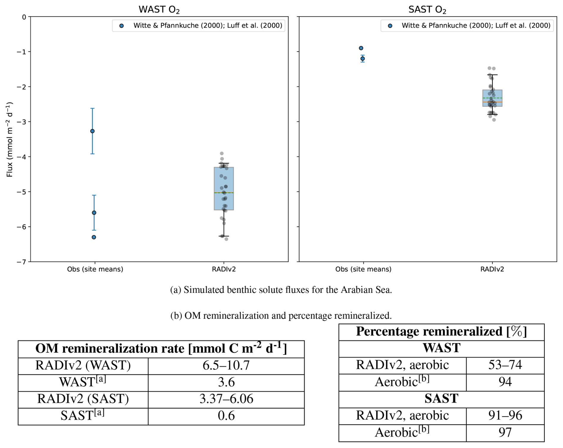
Figure 5 Comparison of simulated benthic solute fluxes and OM remineralization rates with values reported in the literature. (a) Simulated RADIv2 benthic solute fluxes for the Arabian Sea compared to published values. Box–whisker plots compare the distribution of RADIv2 fluxes (“RADIv2”) with observational and modelled site means (“Obs”). The box spans the interquartile range (25 %–75 %), and the whiskers extend to the 5 %–95 % range. The solid orange horizontal line indicates the median, the green dashed line indicates the mean, and coloured jittered dots show individual observations. Where available, the whiskers for the observations indicate the measured standard deviation. Negative O₂ fluxes correspond to uptake of oxygen by the sediment. (b) OM remineralization rates and percentage remineralized values for this study compared to Witte and Pfannkuche (2000) and Luff et al. (2000). ^a Witte and Pfannkuche (2000); ^b Luff et al. (2000).

For SAST, located further from the shelf, the significantly lower POM rain rates lead to lower O₂ fluxes (Fig. 5a), more in line with typical deep-sea O₂ uptake values (Witte and Pfannkuche, 2000). Here, RADIv2 overestimates both O₂ fluxes and remineralization rates, though the model’s aerobic remineralization percentage are consistent with those reported by Luff et al. (2000) (Fig. 5b).

As no DIC measurements were available for these stations, we inferred DIC fluxes using the flux-derived RQ in RADIv2. The simulated RQ is 1.25 for WAST and 1.13 for SAST. Both are higher than those simulated for the Iberian Margin, due to more calcium carbonate dissolution. The values fall within the broader range of RQ values derived from in-situ flux measurements reported for marine sediments by Jørgensen et al. (2022).

3.5 Summary of RADIv2 performance against in-situ observations and published model–data estimates

The simulated ranges of solute fluxes in RADIv2 generally align with values found in the literature, although they are narrower. This narrowing likely results from the steady-state conditions employed in the simulations, which do not account for short-term variability, such as tidal and higher-frequency fluctuations. At some locations, RADIv2 shows a tendency to overestimate benthic fluxes, which likely reflect uncertainties in the prescribed POM supply and organic-matter degradation kinetics. For locations without observed DIC fluxes, the empirical RQ, inferred from benthic DIC and O₂ fluxes, falls within the range of in-situ RQ values reported in the literature (Jørgensen et al., 2022).

However, the model tends to systematically overestimate organic carbon remineralization rates compared to observations. For most sites, the POM rain rates are taken from literature estimates or export–production relationships and are not co-located and time-aligned with the individual in situ flux measurements, so uncertainties in the local POM supply and its degradation kinetics are likely the source of this positive bias. To quantify how much of the disagreement could in principle be absorbed by either the POM flux or the reactivity, we performed three sensitivity tests at the Iberian Margin shallow calibration site, holding all other parameters fixed. Scaling the imposed POM rain by factors 0.5–1.5, while keeping all other organic-matter parameters constant, changes the vertically integrated remineralization rate by roughly −40 % to +40 %, with an almost linear response. In contrast, globally scaling both k_fast and k_slow over a range of 0.5–2.0, while keeping the fast/slow partitioning and POM rain constant, produces smaller and more non-monotonic changes in the integrated rate because faster degradation near the surface reduces the amount of POM transported to depth. Varying the partitioning between the fast and slow pools (while keeping total POM rain and rate constants fixed) only weakly affects the depth-integrated remineralization, but does shift where in the sediment column carbon is oxidized and hence the balance between aerobic and anaerobic pathways. It should be noted that, F_POM, $k_{\mathrm{fast}}/k_{\mathrm{slow}}$ and their partitioning are not independently constrained, and different combinations of these parameters can yield similar total remineralisation rates. These tests indicate that uncertainties in the local POM flux are sufficient to account for much of the overestimation of remineralization, and that global rescaling of the organic matter kinetics and their fast/slow partitioning also affects the integrated rate, but to a lesser degree and more non-linearly. At the same time, the sensitivity tests suggest that RADIv2 is not locked into a “too-reactive” regime. The systematic positive bias across case studies is consistent with uncertainties in the local POM supply, and/or to lesser a extent, the effective reactivity of the sedimentary organic matter.

4 Metamodel

Many GOBMs either oversimplify or completely omit processes governing the exchange of solutes and particulates at the SWI (Carroll et al., 2020; Terhaar et al., 2024; Séférian et al., 2020). This omission can introduce biases in carbon and biogeochemical budgets, particularly in coastal and shelf regions, where sediment dynamics influence water column biogeochemistry (Middelburg and Soetaert, 2004) and thus air-sea gas exchange. The challenge of benthic representation in GOBMs is compounded by the spatial heterogeneity of seafloor sediments (Jørgensen et al., 2022) and variability in key environmental parameters, such as organic matter fluxes and bottom-water concentrations. These complexities make it difficult to apply generic parameterizations across diverse benthic environments, while fully integrating benthic processes into GOBMs is constrained by high computational cost.

To improve the representation of benthic–pelagic coupling in GOBMs, we derive a regression-based metamodel that captures key solute exchange at the sediment–water interface. The metamodel is calibrated by fitting it to RADIv2 benthic fluxes from the ensemble simulations summarized in Table 2 and Figs. 2–5. The metamodel represents benthic solute fluxes as linear functions of five key environmental drivers: bottom-water temperature, current velocity, calcite saturation state, and POC (converted from POM according to redfield stoichiometry (Redfield, 1934)) and PIC deposition fluxes. These predictors were chosen based on experimental, field, and modelling studies that identify them as the dominant physical and biogeochemical controls on benthic DIC, O₂, and TA fluxes. Bottom-water temperature controls molecular diffusion coefficients and the rates of redox reactions (Yuan-Hui and Gregory, 1974), the POC flux drives organic-matter degradation and calcite dissolution (Emerson and Bender, 1981), while PIC concentration and the saturation state govern carbonate dissolution and precipitation (Boudreau, 2013). The current velocity modulates SWI exchange and carbonate kinetics via its effect on diffusive boundary-layer thickness (Boudreau, 2013; Sulpis et al., 2019; Glud et al., 2007), and dispersion (McGinnis et al., 2014). Within the RADIv2 ensemble, these five drivers explain most of the variance in the simulated benthic fluxes across the six calibration sites, while keeping the metamodel compact and compatible with the variables typically available as diagnostics in GOBMs. For the metamodel training ensembles, we set the refractory fraction of particulate organic matter to zero and treat all incoming POC as reactive (assigned to the fast or slow pools), because the POC flux is used directly as a predictor. In RADIv2, refractory organic carbon does not react and therefore does not contribute to benthic solute fluxes, so including a refractory fraction in the training data would introduce ambiguity when applying the metamodel in larger-scale models: if the training was based on a total POC flux that includes a refractory fraction, but the same fraction is not treated consistently in the host model, the predicted benthic fluxes would be systematically biased.

By reducing the complex diagenetic processes simulated by RADIv2 into simplified mathematical relationships that accurately reproduce its outputs, the metamodel provides a robust and scalable representation of SWI exchange, making it well-suited for integration into large-scale ocean models.

The metamodel equations are as follows:

$$\begin{array}{}\text{(21)}& {\displaystyle }\begin{array}{rl}{J}_{\mathrm{DIC}}& =\mathrm{1.84}-\mathrm{0.05}\cdot T-\mathrm{1.68}\cdot U-\mathrm{0.46}\cdot {\mathrm{\Omega }}_{\mathrm{Ca}}\\ & +\mathrm{3.98}\cdot F_{\mathrm{POC}}+\mathrm{1.13}\cdot F_{\mathrm{PIC}},\end{array}\text{(22)}& {\displaystyle }\begin{array}{rl}{J}_{{\mathrm{O}}_{\mathrm{2}}}& =-\mathrm{1.00}+\mathrm{0.0013}\cdot T-\mathrm{4.80}\cdot U+\mathrm{0.17}\cdot {\mathrm{\Omega }}_{\mathrm{Ca}}\\ & -\mathrm{2.90}\cdot F_{\mathrm{POC}}-\mathrm{1.28}\cdot F_{\mathrm{PIC}},\end{array}\text{(23)}& {\displaystyle }\begin{array}{rl}{J}_{\mathrm{TA}}& =\mathrm{1.64}-\mathrm{0.03}\cdot T-\mathrm{8.52}\cdot U-\mathrm{0.53}\cdot {\mathrm{\Omega }}_{\mathrm{Ca}}\\ & +\mathrm{1.67}\cdot F_{\mathrm{POC}}+\mathrm{0.27}\cdot F_{\mathrm{PIC}},\end{array}\end{array}$$

where J_DIC, $J_{{\mathrm{O}}_{\mathrm{2}}}$ and J_TA are the DIC, O₂ and alkalinity sediment fluxes [mmol m⁻² d⁻¹], respectively. Positive fluxes indicate solute release from sediments, while negative fluxes reflect sediment uptake. T is the bottom-water temperature [°C], U is the bottom-water current velocity [m s⁻¹], Ω_Ca is the bottom-water calcite saturation state [–], F_POC is the POC rain rate [mol m⁻² a⁻¹] and F_PIC is the PIC rain rate [mol m⁻² a⁻¹].

Figure 6 compares the simulated benthic solute fluxes for DIC, O₂, and TA from RADIv2 (x-axis) with the corresponding predictions from the metamodel (y-axis). The data points are color-coded by marine environment. The high R² values and relatively low RMSE values demonstrate the metamodel’s ability to accurately reproduce RADIv2 outputs, while also capturing flux variability across diverse marine settings.

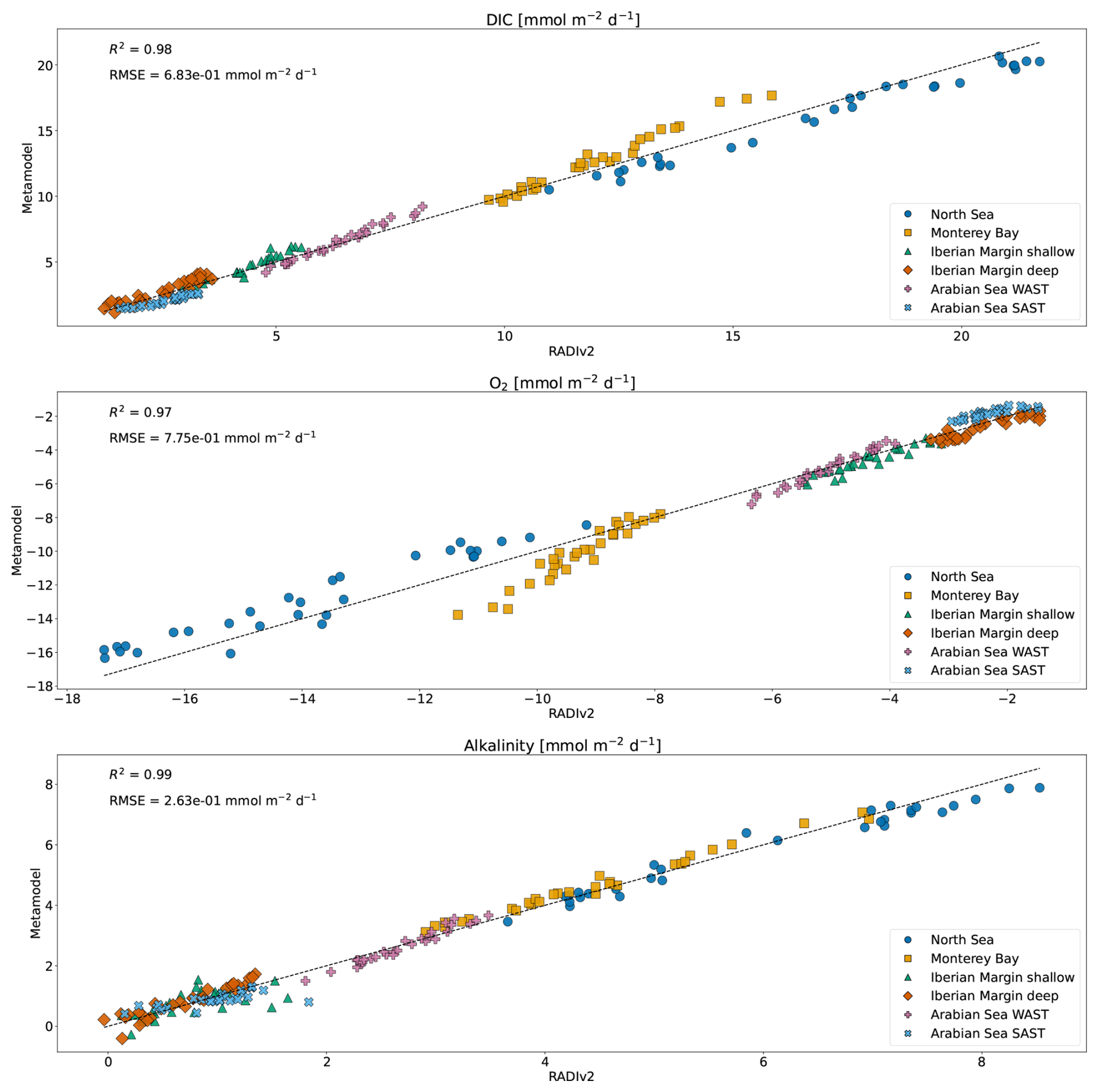
Figure 6 Comparison of RADIv2 simulated benthic solute fluxes (x-axis) with metamodel predictions (y-axis) for DIC, O₂, and TA. Data points are color-coded by marine environment. Positive fluxes indicate solute release from sediments, while negative fluxes reflect sediment uptake.

We performed an offline comparison of the metamodel against in situ benthic flux measurements at the North Sea sites. The metamodel is explicitly designed as a surrogate for RADIv2: its coefficients are calibrated on RADIv2 ensemble outputs and are not tuned directly to observations. Any mismatch with in situ data can therefore be separated into biases and structural limitations in RADIv2 itself, and an additional emulation error introduced by the regression (R²<1 and RMSE >0). To quantify this emulation error and to compare the metamodel directly to both observations and RADIv2, we ran the metamodel with the same bottom-water and depositional drivers used in the corresponding RADIv2 North Sea ensemble set-up (Table 2). Figure 7 compares the resulting metamodel-predicted fluxes with the underlying RADIv2 fluxes and the in situ observations. The metamodel follows the RADIv2 simulations but predicts slightly lower median and mean fluxes at this coastal site, consistent with a single global fit trained across both coastal and deep-sea regimes, which can pull coastal predictions downward toward the fitted mean.

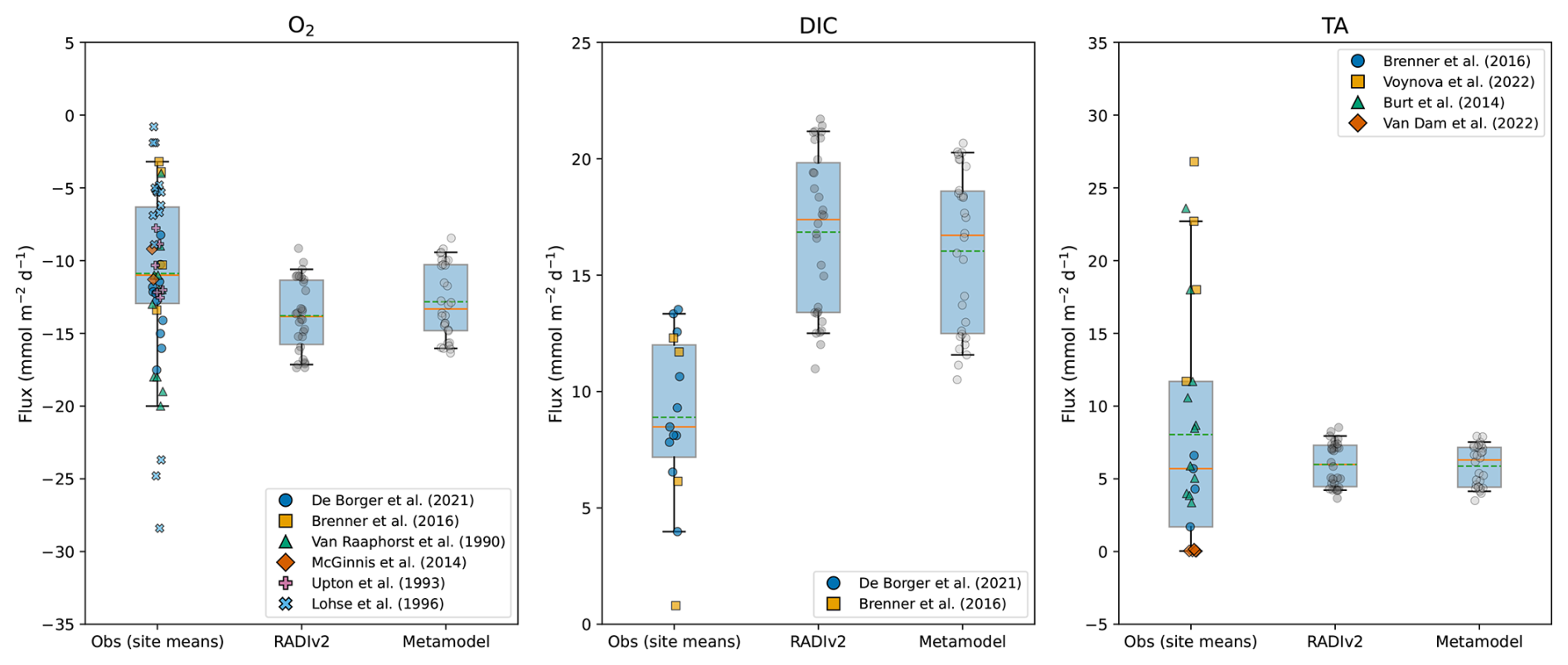
Figure 7 North Sea benthic fluxes of O₂ (left), DIC (middle), and TA (right) from observations, RADIv2, and the metamodel. Box–whisker plots compare the distribution of RADIv2 fluxes (“RADIv2”) with observational and modelled site means (“Obs”). The box spans the interquartile range (25 %–75 %), and the whiskers extend to the 5 %–95 % range. The solid orange horizontal line indicates the median, the green dashed line indicates the mean, and coloured jittered dots show individual observations. Negative fluxes correspond to uptake by the sediment, whereas positive DIC and TA fluxes indicate release to the water column.

5 Discussion and future development

5.1 RADIv2

In RADIv2, diffusive mass transport across the SWI occurs via molecular diffusion in low-permeability sediments, with an additional dispersion term included for highly permeable sediments. This is particularly relevant in coastal sediments, where permeability is typically higher and bottom-water currents are stronger compared to deeper regions, resulting in sediment fluxes that exceed diffusive fluxes alone (Jørgensen et al., 2022). In cases where sediments are sufficiently permeable, a third transport regime, turbulent transport, can contribute to mass transfer across the SWI (Voermans et al., 2018). The transitions between these three regimes (molecular diffusion, dispersive diffusion, and turbulent transport), are characterized by the permeability Reynolds number, $R{e}_k=\sqrt{K}{u}_{*}/\mathit{\nu }$, where K is the sediment permeability, u_* is the shear velocity and ν is the kinematic viscosity. Re_k parameterizes the turbulent regime at the seafloor, with the permeability of the sediments determining whether the turbulence can penetrate through the SWI. A low Re_k indicates a regime dominated by molecular diffusion, while a high Re_k suggests that turbulent transport dominates mass transfer across the SWI. These different regimes can be parameterized by effective diffusion coefficient (Voermans et al., 2018) and can be integrated into future updates of RADIv2. However, the main limitation of this method is its reliance on sediment permeability, a variable property that is challenging to measure in situ. While efforts are underway to map seabed permeability in coastal regions (Moosdorf et al., 2024), a global dataset for linking permeability to RADIv2 is not yet available. A transient test case with tidal currents (Supplement Sect. S2, Fig. S2) illustrates how the present formulation in RADIv2 translates such hydrodynamic forcing into time-varying benthic O₂ fluxes.

Future efforts will focus on improving the representation of organic carbon degradation kinetics, a key driver of sediment fluxes. Currently, RADIv2 divides organic carbon into two reactive classes (k_fast and k_slow), each following first-order reaction kinetics. This approach to organic matter degradation produces a vertical structure in bulk (apparent) reactivity: the more labile pool is consumed near the sediment–water interface, so deeper layers are dominated by less reactive carbon. This is sufficient for well-mixed sediments, where organic carbon reactivity is relatively constant within the mixed layer (Kuderer and Middelburg, 2024). However, experimental studies (Westrich and Berner, 1984), field observations (Jorgensen, 1978), and recent theoretical advances (Rothman, 2024) have shown that organic carbon reactivity often declines with degradation. In RADIv2 each organic-matter pool has a fixed degradation rate constant, and degradation does do not weaken with depth or time. The work of Kuderer and Middelburg (2024) summarizes the conditions under which different degradation kinetics are suitable, and highlights the need to model organic carbon reactivity as a continuum that declines with age and burial depth in regions that receive highly reactive OM or poorly-mixed environments, rather than a small number of fixed-k pools. Incorporating such an approach into RADIv2 would enhance its ability to simulate organic matter degradation under a broader range of marine sediments. Future work could focus on dynamically adjusting organic matter degradation kinetics based on the sediment mixing regime (quantified by the Péclet number) and the reactivity of incoming organic carbon. This would also help address the current overestimation of organic matter degradation rates by better capturing the declining reactivity of organic carbon over time, providing more accurate remineralization estimates.

Fluxes across the sediment–water interface are controlled by processes that are strongly concentrated in the upper centimetres of the sediment, so the vertical grid spacing must be sufficiently fine to resolve the associated reaction and concentration gradients. Future applications of RADIv2 could benefit from a non-uniform vertical grid, with finer spacing near the sediment–water interface and coarser spacing at depth, particularly in coastal sediments or simulations that require a deeper sediment column. RADIv2 is a living model, and ongoing developments focus on supporting non-uniform grids (for example, with finer dz near the SWI and coarser spacing at depth) to further improve the efficiency of simulating of near-surface processes.

Both RADIv1 and RADIv2 are optimised for simulating carbon and oxygen cycling. In the present configuration, RADIv2 includes dissolved Fe²⁺ and Mn²⁺ and their oxidised solid phases, and represents their role as electron acceptors in organic-matter degradation. However, it does not resolve a full Fe–Mn–S mineral network. Sulfide produced by sulfate reduction is treated with simplified oxidation and precipitation terms (see Table 1), and processes such as explicit FeS/pyrite formation, burial and re-oxidation are not included. These missing pathways can be important for the alkalinity budget in iron-rich, bioturbated coastal sediments, because they control whether sulfide is buried as pyrite or repeatedly re-oxidised and recycled back to sulfate through Fe–S redox cycling, and these alternative pathways have different net TA yields (Canfield et al., 2005). Future extensions of RADIv2 should focus on implementing more comprehensive iron and manganese cycles with explicit sulfide–mineral pathways, following formulations such as Fossing et al. (2004) and Canfield et al. (2005), to improve applications in such settings.

RADIv2 was designed with extensibility in mind, providing a flexible and adaptable framework that makes the addition of new components or species straightforward. Moreover, RADIv2 can be updated to represent specific environments, such as mangrove forests, estuaries, or nearshore intertidal zones. This versatility enables RADIv2 to serve as a robust foundation for advancing future diagenetic research across a wide range of applications.

5.2 Metamodel

Significant discrepancies exist between estimates of the ocean carbon sink derived from pCO₂ products and those produced by ocean biogeochemical models (Friedlingstein et al., 2023; DeVries et al., 2023), which are further complicated by inter-model variability (Terhaar et al., 2024). One major uncertainty comes from the poor representation of particulate deposition at the seafloor and the resulting benthic fluxes from remineralization, dissolution, and exchange at the SWI. The exclusion of sediment-seawater exchange processes in current models limits their ability to accurately simulate coastal-ocean productivity and air-sea gas exchange as benthic processes play an important role in nutrient recycling and carbon dynamics (Middelburg and Soetaert, 2004), particularly in shallow regions where the seafloor and bottom waters directly interact with the surface layer. An analysis by Séférian et al. (2020) of the marine biogeochemical components in CMIP5 and CMIP6 Earth System Models (ESMs) reveals that most CMIP5 models lacked any representation of sediments. While CMIP6 models have made significant progress incorporating sediment processes, their treatment remains highly simplified and, in some cases, is still omitted. When sediments are not explicitly represented, particulates that reach the seafloor are either instantaneously remineralized (Swart et al., 2019) or permanently buried upon deposition (numerically lost) (Aumont and Bopp, 2006; Carroll et al., 2020). Most ESMs that include sediments rely on a box-model approach, where organic matter reaching the seafloor is either remineralized or buried based on simplified relationships with downward organic fluxes. Some ESMs estimate organic matter remineralization through denitrification following the formulation of Middelburg et al. (1996) (Stock et al., 2020; Aumont et al., 2015), with additional pathways for aerobic respiration or sulfate reduction (Stock et al., 2020). More advanced sediment models, such as those incorporated in HAMOCC and PISCES-v2 (Ilyina et al., 2013; Mauritsen et al., 2019), adopt a layered sediment module based on Heinze et al. (1999). While this represents a significant step forwards, these models still rely on highly simplified treatments of key diagenetic processes. Important mechanisms, such as bioturbation (irrigation), dispersion, and anaerobic organic matter degradation are either absent or not fully accounted for.

Since RADIv2 is developed in Julia, while ESMs are typically written in FORTRAN, direct coupling is not straightforward without significant code translation. Additionally, fully kinetic diagenetic models like RADIv2 are computationally intensive, making their real-time integration into Earth System Models currently unfeasible. This study introduces a process-based metamodel that captures key diagenetic processes, often oversimplified or absent in existing parameterizations, without requiring full integration.

The metamodel is validated for diverse marine environments, accurately reproducing SWI exchanges simulated by RADIv2. By accounting for the heterogeneity and variability in sediment properties and environmental conditions, the metamodel is designed for broad applicability. However, the present training and validation set primarily samples temperate shelves, margins, and deep-sea settings, and does not explicitly include environments such as deltaic systems, very shallow nearshore regions, or carbonate-rich tropical shelves. Expanding the training ensemble to a wider, yet physically consistent, range of bottom-water conditions and particulate fluxes, that can also be validated with in-situ observations, represents an important future improvement, especially for more localized applications. The flexibility of RADIv2 allows for customization to specific marine environments, such as bays and estuaries, when region-specific data are available, enabling either the expansion of the present metamodel or the generation of specialized metamodels for regional applications.

Future work will focus on expanding the metamodel to include additional particulate fluxes, such as particulate metallic fluxes, and on parameterizing the corresponding SWI exchange. Ongoing developments will also expand the range of solute fluxes covered by the metamodel, including phosphate, nitrate, ammonium, methane, and particulate organic and inorganic carbon fluxes. This expansion is expected to improve biogeochemical budget estimates, as the lack of sediment regeneration of nutrients from remineralized organic matter can lead to underestimation of primary production in biogeochemical models (Yool et al., 2013; Liu et al., 2007). The adaptability of the RADIv2 framework allows the approach presented here to be extended to develop metamodels for any solute or particulate flux included in RADIv2, facilitating its application across diverse marine environments and geochemical processes.

6 Conclusions

RADIv2 is a versatile diagenetic model designed to simulate sediment-water interface (SWI) exchanges across a range of marine environments. Built using Julia’s DifferentialEquations.jl package, RADIv2 leverages high-performance capabilities and an adaptive structure to address the complexity and variability of sediment processes. A key feature of RADIv2 is the flexibility of its framework, which allows for adaptation to specific environmental conditions and simulation setups. This capability enables optimization for diverse marine environments, from dynamic coastal regions to stable deep-sea sediments. The ensemble simulation feature in RADIv2 constrains variable environmental parameters, such as bottom-water temperature, currents, and particulate export fluxes, by generating statistical envelopes that capture variability, better reflecting the natural fluctuations observed in in situ measurements over time and helping to reduce uncertainty in model inputs. This approach enhances the model’s ability to represent the heterogeneity of marine sediments. RADIv2 also includes an optimization scheme for tuning model parameters based on in-situ observations, further improving model accuracy. Simulated solute fluxes in RADIv2 across various marine environments generally align with observed values from the literature, though the narrower variability reflects the model’s steady-state assumptions. Despite this, mean fluxes and empirically derived RQ values remain consistent with in-situ data, indicating that RADIv2 provides robust estimates of benthic fluxes over longer timescales. However, the model tends to overestimate organic carbon remineralization rates.

Using RADIv2 outputs, we developed a metamodel that parameterizes benthic-pelagic coupling with a simplified set of equations. These equations accurately capture steady-state benthic solute fluxes linked to the marine carbon budget across various environments, accounting for sediment heterogeneity and environmental variability. The metamodel builds on a comprehensive diagenetic framework that incorporates detailed sedimentary processes, without the high computational demands of fully coupled water column-sediment biogeochemical models at the global scale. This ensures more accurate processing of particulates at the seafloor and accounts for the exchange of remineralization and dissolution products between sediments and bottom waters. Ultimately, this metamodel offers a pathway for more accurate representations of benthic-pelagic coupling in global ocean biogeochemistry models, improving estimates of ocean biogeochemical cycling.