Implementation of a multi-layer snow scheme in the GloSea6 seasonal forecast system: impacts on land–atmosphere interactions and climatological biases

This study explores the influence of implementing a multi-layer snow scheme on the climatological bias within a seasonal forecast system. Traditional single layer snow schemes in land surface models, particularly those utilising a composite snow-soil layer, often inadequately represent the insulating effect of snowpack, resulting in cold and warm biases during winter and snowmelt seasons, respectively. By contrast, multi-layer snow schemes improve the simulation of energy exchange between the land surface and atmosphere by realistically capturing snowpack thermal processes. To examine this impact, two sets of LSM offline experiments are conducted, using either a single-layer or a multi-layer snow scheme. Results show that the multi-layer configuration better reproduces the observed Northern Hemisphere snow seasonality. To further assess the role of snow insulation in coupled forecast systems, two sets of experiments with the Global Seasonal Forecast System (GloSea) version 6 are compared over 24 years (1993–2016) corresponding to the incorporation of single- (G6_single) and multi-layer (G6_multi) snowpack schemes. In G6_multi, the onset of snowmelt is delayed by approximately 1–2 weeks, postponing springtime evaporation, slowing soil moisture depletion, and improving the memory of soil moisture. Increased soil moisture enhances the partitioning of available energy into latent heat flux, thereby promoting evaporative cooling and suppressing excessive water-limited land–atmosphere coupling. The improved model fidelity of land-atmosphere interactions, particularly over mid-latitude regions, mitigate near-surface warming biases across the entire diurnal period and reduce the sensitivity of atmospheric conditions to land surface variability. The model performance in simulating precipitation is also improved with the increase in precipitation occurrence over snow-covered regions. Above all, this study demonstrates the value of implementing a multi-layer snowpack scheme in seasonal forecast models, not only during the snowmelt season but also for the subsequent summer season, for model fidelity in simulating temperature and precipitation along with the reality of land-atmosphere interactions.

1 Introduction

Subseasonal-to-seasonal (S2S) forecasts have become increasingly pivotal in numerous fields, encompassing agriculture, water resource management, energy, transportation, and disaster preparedness. The significance of S2S forecasting stems from their ability to provide actionable insights into forthcoming weather and climate conditions over the span of weeks to months. The predictability of S2S forecasts is strongly tied to the quality of the initial conditions and data assimilation technique, which mathematically finds optimal values with minimized analysis errors to merge observations into a dynamical model, has been employed to create improved global analyses (Seo et al., 2021; Kumar et al., 2022). Forecasts across various time scales underscore the necessity for precise initial states of distinct components within the forecast model, as each component retains information over inherently disparate time scales (Richter et al., 2024). As the memory of initial land conditions can extend out to approximately 2 months, the importance of realistic land surface initialization in determining skill of the subseasonal forecast is paramount (Koster et al., 2011; Guo et al., 2011; Seo et al., 2019).

In particular, soil moisture (SM) plays a pivotal role in hydrological and meteorological dynamics, acknowledged as an essential climate variable by the World Meteorological Organization (WMO) (Seneviratne et al., 2010; Santanello et al., 2018). Its persistence or memory can significantly enhance forecast accuracy, particularly at time scales extending to 1–2 months (Dirmeyer et al., 2016, 2018; Seo and Dirmeyer, 2022a). The fidelity of modelled SM contributes to a more accurate portrayal of land-atmosphere interactions, facilitating the exchange of water and energy fluxes at the land surface (Seo et al., 2024). This enhanced representation holds potential for predicting extreme climate events, particularly those intensified by land-atmosphere feedback within extended range forecast systems (Seo et al., 2020; Tak et al., 2024; Dirmeyer et al., 2021). SM is directly constrained by the components of the typical water balance equation: precipitation, latent heat flux, and runoff, but the modelled snow affects the representation of snow characteristics.

The pivotal role of snow in land-atmosphere interactions highlights the significance of accurately representing cold processes related to snow in hydrometeorology and dynamical predictions. Compared to other land surface variables, snow exhibits distinctive characteristics such as high albedo, high thermal emissivity, and low thermal conductivity, which profoundly influence radiation budget and surface moisture and energy fluxes to the atmosphere. The presence or absence of snow can result in a disparity of approximately 10 K in the climatology of surface air temperature (Betts et al., 2014). This discrepancy primarily stems from the reduction in net shortwave radiation attributable to the high albedo of snow. Snow-atmosphere feedback evolves through three distinct stages: before, during, and after snowmelt. Meanwhile, the coupling strength of snow cover to near-surface atmospheric variables, as measured by the phase similarity of members of an ensemble forecast induced by specifying identical land surface conditions (Koster et al., 2006), is strongest during snowmelt and the coupling strength after snowmelt (delayed soil moisture impact) is stronger than that before snowmelt (radiative impact from surface albedo) (Xu and Dirmeyer, 2011). Therefore, during the warm season, SM dynamics become intricately linked to the physical characteristics of snow, affecting the initiation of evaporation and runoff due to snowmelt. It plays a crucial role in determining the model's ability to accurately simulate atmospheric variables through land-atmosphere coupling processes.

Some Land surface models (LSMs) still use a single-layer snowpack scheme, which has proven insufficient in accurately capturing the seasonal evolution of snow cover. The snowpack insulates the land surface, inhibiting energy exchange between the land surface and the atmosphere. Consequently, a single layer snowpack scheme typically leads to cold and warm biases during winter and snow melting seasons, respectively. While single-layer schemes can theoretically account for insulation through adjusted thermal resistance, implementations that combine snow and the uppermost soil layer into a single thermal store (as used in the control experiment of this study) cannot represent a vertical temperature gradient within the snowpack. Consequently, in such composite configurations, surface temperature changes are transmitted directly to the soil below, enhancing the efficiency of energy exchange. Addressing these limitations, recent advancements in LSMs aim to integrate the multi-layer snow scheme to enhance the representation of snow dynamics and mitigate associated biases. For instance, Noah-Multiparameterization (Noah-MP) LSM represents the latest iteration of Noah LSM, a land component widely implemented with a single layer snowpack in various regional and global operational forecast models. It incorporates multiple enhancements aimed at improving the realism of biophysical and hydrological processes (Niu et al., 2011). Notably, for a more accurate representation of snow physics, Noah-MP adopts the multi-layer snowpack scheme. This scheme dynamically adjusts the number of snow layers based on the depth of snow, ensuring a more realistic conceptualization of snow accumulation and melt processes. The Joint UK Land Environment Simulator (JULES) LSM features the utilization of a multi-layer snow scheme in its current operational system. It also dynamically adjusts the number of snow layers, with each layer having prognostic variables for temperature, density, grain size, and both liquid and solid water content (Best et al., 2011). Unlike the simpler single layer snow model, which treats snow as an adaptation of the top-soil layer, the multi-layer scheme accounts for independent snow layer evolution and the impact of snow aging on albedo through simulated grain size changes. By explicitly simulating snow insulation effects and meltwater percolation, this scheme better captures seasonal snow variability and its influence on soil thermal regimes, including surface cooling during winter, delayed ground thaw in spring, and subsurface heat retention in summer. This implementation significantly improves soil temperature simulations, leading to better representation of land surface processes (Burke et al., 2013; Walters et al., 2017). JULES is incorporated within the GloSea forecast system (MacLachlan et al., 2015).

Numerous studies have aimed to improve the sophistication of snow physics and highlighted its advancement in numerical models (Xue et al., 2003; Arduini et al., 2019; Cristea et al., 2022). For instance, among 13 operational models participating in sub-seasonal to seasonal (S2S) prediction project (Vitart et al., 2017, 2025), only three – BoM (POAMA P24), CNR-ISAC (GLOBO), and NCEP (CFSv2) – employ a single-layer snowpack scheme, whereas the remaining ten models, including those developed by CMA (BCC-CPS-S2Sv2), CNRM (CNRM-CM 6.1), CPTEC (BAM-1.2), ECCC (GEPS8), ECMWF (CY49R1), HMCR (RUMS), IAP-CAS (CAS-FGOALS-f2-V1.4), JMA (CPS3), KMA (GloSea6-GC3.2), and UKMO (GloSea6), now used multi-layer snowpack schemes. Despite this broad adoption, the impact of multi-layer snow schemes on S2S forecasts remains insufficiently explored and understood. Hence, this study conducts a comparative analysis between single layer and multi-layer snowpack in the JULES LSM, as well as the fully coupled forecast systems GloSea5 and GloSea6 – past and present operational forecast systems at the UK Met Office and the Korea Meteorological Administration (KMA), in retrospective forecasting in order to investigate the impact of an advanced snow scheme. The primary objective of this study is to assess the seasonal cycle of snow and land surface variables throughout the snow-covered period and evaluate the model's capability to replicate the mean climatology of key land surface and near-surface atmospheric variables, e.g., surface SM, surface air temperature, and precipitation, during the boreal warm season. The evaluation is restricted to the Northern Hemisphere (NH) and mainly to snow-affected mid-latitude regions. Daily mean, maximum, and minimum temperatures are validated at sub-daily time scales to elucidate the time of significant improvements in model performance. Furthermore, the model fidelity in the simulation of land-atmosphere interactions, corresponding to water- and energy-limited processes, is diagnosed to identify the realism of land coupling regimes by implementing the advanced snowpack scheme.

The paper is organized as follows. Section 2 describes the GloSea5 and GloSea6 models, and the validation datasets used in this study. Section 3 provides the methodology to evaluate the model performance. Section 4 presents and discusses the results of this study. Finally, Sect. 5 summarizes the results and their implications for future applications.

2 Model Description and Data

2.1 Forecast Model

This study explores the performance of the Global Seasonal forecast system (GloSea) version 5 and 6, which are abbreviated as GloSea5 and GloSea6, respectively. These are the fully coupled ensemble forecast models with atmosphere-land-ocean-sea ice components, developed by the UK Met Office. GloSea5 (MacLachlan et al., 2015) Global Coupled model 2.0 (GC2; Williams et al., 2015) configuration consist of UM (Unified Model) version 8.6 atmospheric component (GA6.0; Walters et al., 2017) having N216 horizontal resolution of 0.56° latitude × 0.83° longitude with vertically 85 hybrid-sigma coordinates topped at 85 km, JULES (Joint UK Land Environment Simulator) version 4.7 land surface model (GL6.0; Best et al., 2011) with four soil layers (0–10, 10–35, 35–100, and 100–300 cm depth), as well as NEMO (Nucleus for European Modelling of the Ocean) version 3.4 oceanic component (GO5.0; Megann et al., 2014) and CICE (Los Alamos Sea-ice Model) version 4.1 sea-ice component (GSI6.0; Rae et al., 2015) on an ORCA tripolar 0.25° global grid with 75 vertical levels. Those components exchange interactive variables with the OASIS3 coupler (Valcke, 2013). GloSea6 Global Coupled model 3.2 (GC3.2) updates the atmospheric, land, ocean, and sea-ice components to the version of UM vn11.5 (GA7.2), JULES vn5.6 (GL8.0; Wiltshire et al., 2020), NEMO vn3.6 (GO6.0; Storkey et al., 2018), and CICE vn5.1.2 (GSI8.1; Ridley et al., 2018) without any modification in the resolution. The model components of GloSea6 are coupled with the OASIS3-MCT (Model Coupling Toolkit; Craig et al., 2017).

Substantive changes in the GloSea6 compared with GloSea5, mostly in model physics, have been implemented throughout all model components (Williams et al., 2015, 2018). For instance, the atmospheric physics are modified in radiation (improving gaseous absorption through upgrades in McICA (Monte Carlo Independent Column Approximation) and parameterization in ice optical properties), microphysics (updates in warm rain parameterization and newly implementing ice particle size-dependent parameterization), cloud physics (including radiative effects from convective cores), gravity wave drag (implement heating from gravity-wave dissipation), boundary layer (correcting cloud top entrainment during decoupling to the land), cumulus parameterization (improving updraught numeric in convective process and updating CAPE closure as a function of large-scale vertical velocity), and new modal aerosol scheme (UKCA GLOMAP (Global Model of Aerosol Processes) scheme; Mann et al., 2010). Aforementioned atmospheric physics updates in the GloSea6 are likely to improve the performance of model systemic errors, particularly in the overestimated vertical profile of cloud fraction at upper troposphere, tropospheric cold and dry biases, the underestimated jet stream, the overestimated precipitation, and the negative bias of troposphere geopotential height during boreal summer (Williams et al., 2018).

Land surface types in the both forecast systems are classified with five vegetation (broadleaf trees, needleleaf trees, C₃ grasses, C₄ grasses and shrubs) and four non-vegetated surfaces (urban, open water, bare soil and permanent land ice) and the monthly climatology of leaf area index, derived from MODIS satellite product (Yang et al., 2006), is prescribed corresponding to the plant functional types. However, in GloSea6, there are two major updates in land physics: the implementation of a multi-layer snow scheme and the realization of shortwave surface albedo. GloSea5 employs a single-layer snow scheme using a composite approach, in which the snow and the uppermost soil layer are combined into a single thermal store (Best et al., 2011). Because the snow and top-soil layer share the same prognostic temperature, the scheme effectively allows direct heat exchange between the surface atmosphere and the soil, limiting the representation of a thermal gradient through the snowpack. It combines the snow and the uppermost soil layer into a single thermal store, with the increased snow depth leading to a reduction in the effective thermal conductivity. This reduction is not a dynamic representation of the intrinsic properties of snow but rather an adjustment to account for the insulating effect of the snow. This scheme lacks proper closure of the surface energy budget (Fig. S1 in the Supplement) and a dynamic representation of snowpack evolution with the inadequate depiction of the snowpack's insulating properties. The improvement from the implementation of the multi-layer snow scheme is shown not only in the realization of the snow melt season, but also in the soil temperature and permafrost extent (Walters et al., 2019). For instance, the multi-layer snow scheme leads to surface warming of the soil temperature during the winter season, as the heat flux from the soil to the atmosphere is reduced, but shows a surface cooling in the spring season, as the increase in insulating radiation inhibits snowmelt. In the snow frontal regions, the increase in land surface albedo is due to the delay in the onset of snowmelt by the multi-layer snowpack.

In both forecast models, the snow-free surface albedo for each grid box is calculated as a weighted average of the albedos of different surface types, with MODIS bare soil albedo (Houldcroft et al., 2009) and GlobAlbedo surface albedo in other non-vegetated surface types (Muller et al., 2012). The albedo of vegetated surface types is defined as a combination of the bare soil albedo and the full leaf albedo, with the weighting determined by the leaf area index (LAI) of the respective vegetation type. In GloSea6, to improve surface albedo representation, these albedos are modified as a function of shortwave wavelength. Since surface albedos, which are independent of wavelength, limit spectral variability, photosynthetically active radiation (PAR) and near-infrared radiation (NIR) are calculated separately using the canopy radiation model (Sellers, 1985). In addition, the generation of the surface albedos of land surface types is amended. The mapping from the International Geosphere Biosphere Programme (IGBP; Loveland et al., 2000) classification to JULES land surface types has been refined in GloSea6. The proportion of bare soil within the grassland, cropland, and crop-natural mosaic the IGBP classes was reduced and the coverage of vegetated land types, especially for C₃ grass cover is extended (Walters et al., 2019; Wiltshire et al., 2020). The shift from bare soil to vegetated surfaces decreases surface albedo (Fig. 2e), as the vegetation can penetrate snow cover during the winter season. Therefore, the surface albedo differences observed during the snow-covered season can be attributed to amendments in land surface type classification, whereas the albedo differences during the snow-free period are understood to result from the incorporation of wavelength-dependent calculations in the surface albedo scheme. Other land surface physics are consistent in GloSea5 and GloSea6.

In terms of initial conditions for each model component, GloSea5 and GloSea6 commonly utilize ERA-interim and a variational data assimilation system for the NEMO ocean model (NEMOVAR; Mogensen et al., 2012) analysis for the atmospheric and ocean and sea-ice initializations, respectively. Land surface reanalysis, where the land offline simulation is forced by atmospheric boundary conditions from Japanese 55 years Reanalysis (JRA-55; Kobayashi et al., 2015) and European Centre for Medium-Range Weather Forecasts (ECMWF) Reanalysis version 5 (ERA5; Hersbach et al., 2020), is used to initialize land surface variables for GloSea5 and GloSea6, respectively. GloSea5 and GloSea6 have been used to carry out 60 d (depending on ensemble or variable, 6-month forecast is conducted for the seasonal prediction) retrospective forecasts starting on the 1st, 9th, 17th, and 25th of every month for 26 years (1991–2016) and 24 years (1993–2016), respectively, but evaluations are conducted with 24-year forecasts for the fair comparison between both systems. To operate ensemble forecasts, the Stochastic Kinetic Energy Backscatter (SKEB2; Tennant et al., 2011) and the Stochastic Perturbation of Tendencies (SPT; Sanchez et al., 2016) schemes are used to perturb initial states in GloSea5 and GloSea6, respectively. Compared to the SKEB2, the SPT scheme imposes additional constraints on energy and water conservation, leading to an increase in the spread of ensemble without degrading ensemble mean fields, which is especially beneficial over the tropics. Based on these methods, GloSea5 and GloSea6 operate 3 and 7 ensemble forecasts and have been implemented by the KMA in international S2S prediction project for 2020–2022 and 2023–present, respectively.

To solely understand the impact of the multi-layer snowpack scheme in a fully coupled forecast system, we have carried out another experiment by implementing a single layer snowpack scheme in GloSea6. We have conducted 6-month long retrospective forecasts with a 4-member ensemble initiated on 1 March for 24 years (1993–2016). Throughout this paper, we refer GloSea5, GloSea6 and GloSea6 with a single-layer snow scheme to G5_single, G6_multi and G6_single, respectively. The description of model configurations is summarized in Table 1.

Table 1 Description of the G5_single, G6_multi, and G6_single model configurations.

2.2 JULES offline experiments

To explore the impact of the multi-layer snowpack scheme on land-atmosphere coupling processes in coupled and uncoupled (land only) model configurations, we further conduct two sets of LSM offline experiments using GL8.0 (representing a specific configuration of JULES version 5.6 within the coupled system): implementing single layer (JULES_single) and multi-layer (JULES_multi) snowpack schemes, respectively. The offline LSM simulations are driven by observed atmospheric near-surface variables, including 2 m air temperature and humidity, 10 m wind speed, downward radiative fluxes, and pressure at the surface. These historical observations are employed by the hourly ERA5 reanalysis (Hersbach et al., 2020). Precipitation is forced by the hourly averaged Integrated Multi-satellitE Retrievals for GPM (IMERG) version 7 (Huffman et al., 2023). Both offline experiments are conducted over global land areas from January 2001 to December 2022 at a spatial resolution of 0.56° latitude × 0.83° longitude, consistent with the resolution of the fully coupled forecast systems.

The single layer scheme represents snow as a modification of the uppermost soil layer, applying a fixed thermal conductivity without explicitly resolving vertical snow structure. This simplification results in direct heat exchange between the surface and soil, leading to excessive soil cooling in winter and rapid warming during spring melt. In contrast, the multi-layer scheme explicitly represents up to three snow layers with predefined layer thicknesses of 0.04, 0.12, and 0.34 m, dynamically adjusting the number of active layers based on snow depth (Best et al., 2011). It incorporates a density-dependent thermal conductivity parameterization, improving the simulation of snow insulation effects and reducing soil temperature biases. Additionally, the multi-layer scheme includes a prognostic snow densification process driven by overburden stress and temperature, while also explicitly handling meltwater retention, percolation, and refreezing. Snow albedo is also treated with a prognostic approach that accounts for snow aging and grain size evolution, enhancing radiative feedback representation. Lastly, the multi-layer snowpack ensures surface energy budget closure by explicitly solving for the energy balance of each snow layer, addressing limitations in the single layer scheme that can lead to inconsistencies in snowmelt partitioning.

2.3 Validation Data

The daily maximum and minimum temperature over land at a height of 2 m are sourced from NCEP CPC analysis produced by NOAA Physical Sciences Laboratory (PSL; https://psl.noaa.gov, last access: 3 February 2026). The temperature data have a 0.5° horizontal resolution and are available for 1979–present. The daily mean temperature is acquired by arithmetically averaging maximum and minimum temperature. Hereafter, daily mean, maximum, and minimum temperature will be referred to as T_mean, T_max, and T_min, respectively.

The ERA5-Land is an offline land reanalysis (Muñoz-Sabater et al., 2021) of the Tiled ECMWF Scheme for Surface Exchanges over Land incorporating land surface hydrology (H-TESSEL) land surface model with four soil layers (0–7, 7–28, 28–100, and 100–289 cm depth), forced by the ERA5 atmospheric reanalysis. ERA5-Land has a horizontal resolution of ∼ 0.08° and an hourly temporal resolution. To enhance the spatial resolution of the ERA5-Land, ERA5 near surface atmospheric variables (e.g., temperature, humidity, and pressure) used for boundary conditions are corrected to account for the altitude difference that came from the lower resolution of ERA5.

This study uses Japanese Reanalysis for Three Quarters of a Century (JRA-3Q; Kosaka et al., 2024) as a reference for snow water equivalent (SWE) to diagnose the modelled snow. It employs an offline version of the Simple Biosphere (SIB) model (Sellers et al., 1986). Compared to the satellite-based and in situ datasets, the snow cover and depth are accurately described in its predecessor, the Japanese 55-year Reanalysis (JRA-55) (Orsolini et al., 2019). JRA-3Q incorporates daily snow depth data from the Special Sensor Microwave/Imager (SSM/I), the Special Sensor Microwave Imager Sounder (SSMIS), and in situ measurements using a univariate two-dimensional optimal interpolation (OI) approach. Although this procedure is comparable to that used in JRA-55 (Kobayashi et al., 2015), two issues – unrealistic analysis near coastal areas and unintended increments caused by satellite data biases – have been resolved in JRA-3Q. Additionally, JRA-3Q employs the multi-layer snowpack scheme whereas JRA-55 uses a single layer snowpack scheme. JRA-3Q has a horizontal resolution of 0.375° and 3-hourly temporal resolution.

A time-filtered satellite product of daily surface SM, originated from the COMBINED European Space Agency (ESA) Climate Change Initiative (CCI) Soil Moisture v08.1 dataset (Dorigo et al., 2017), is used to assess the global SM memory (SMM) simulated by forecast models. Remotely sensed SM datasets inherently contain random and periodic errors, particularly in high-frequency variability, due to the radiometric instrument performance, viewing angle variations, spatial resampling, imperfect parameterizations used in retrieval algorithms, and so on. Due to these errors, the daily time series of satellite-based SM retrieval often shows intervals with an increase in SM without rainfall or any other water supply (see Fig. 6 in Seo and Dirmeyer, 2022a), which is unexplainable by the surface water budget. This erroneous SM behavior hampers the representation of realistic SM dynamics and land-atmosphere interactions due to a decrease in the SM autocorrelation value. Since the SMM is calculated with the time-lagged SM autocorrelation, assuming that the daily SM time series is exponentially decaying, the inherent error in the satellite data leads to an underestimation of SMM. To avoid the problem, this study uses the time-filtered surface SM product covering 21 years (2000–2020) with 0.25° spatial resolution, using a Fourier transform with LSM datasets (Seo and Dirmeyer, 2022a). The time-filtered SM product provides a better representation of the surface SM time series, which also contributes to the improvement of the SM characteristics (i.e., SM memory and error) compared to the result from in situ observations. Hereafter, we refer to the adjusted ESA CCI SM based on the LSM simulations as ESACCI_adj.

The Global Land Evaporation Amsterdam Model version 4 (GLEAM; Miralles et al., 2025) provides a dataset of global terrestrial heat fluxes and soil wetness. It combines satellite observations, reanalysis products, and in situ data using a hybrid modelling framework that includes physical principles and machine learning-based estimations of evaporative stress. Based on the Penman's equation, GLEAM estimates potential evaporation using additional atmospheric control factors (e.g., wind speed, vapor pressure deficit, and vegetation height) not only for net radiation and near-surface air temperature observations. Actual evaporation is then derived by applying a multiplicative evaporative stress factor, calculated from observed Vegetation Optical Depth (VOD) and estimated root-zone soil moisture. The GLEAM dataset demonstrates reliable performance in capturing observed seasonal cycles, particularly in evaporation anomalies across diverse climates, when evaluated against global eddy-covariance flux tower observations. Compared to other datasets (e.g., ERA5-Land and FLUXCOM), the GLEAM shows improved agreement with observations. Although the GLEAM performs better than other available reanalysis datasets, it should not be considered an observational dataset. GLEAM estimates evaporation using training data from flux tower observations; however, these towers are mainly ecological monitoring networks that are skewed toward wetter vegetated sites. As a result, while GLEAM is generally reliable in wetter areas, its accuracy in drier regions may be limited due to sparse observational constraints. Nevertheless, since this study focuses on mid- and high-latitude regions where flux towers are plentiful, snow processes dominate and GLEAM's performance is more robust, it is used as the primary reference dataset. Accordingly, to evaluate model performance, this study utilizes the daily surface SM, evaporation, sensible heat flux, and net radiation (defined as the sum of latent and sensible heat fluxes) from version 4.2a (https://www.gleam.eu/, last access: 3 February 2026), covering 44 years (1980–2023) with a 0.1° spatial resolution.

The Multi-Source Weighted-Ensemble Precipitation (MSWEP) version 2.8 is the gauge-, satellite-, and reanalysis-based precipitation dataset used for validation, available from 1979 to the present. The precipitation data have a 0.1° horizontal resolution and 3-hourly temporal resolution (Beck et al., 2019a). Its superior performance is primarily attributable to the inclusion of daily gauge observations compared with 26 gridded precipitation datasets (Beck et al., 2019b).

3 Methodology

This study aims to investigate the impact of an improved snow scheme in the seasonal forecast system on the fidelity of snow behavior contemporaneously and during the next warm season after snow melt. To compare model performance between G6_multi and G5_single for analyzing the climatology of the seasonal cycle, 100 d long retrospective forecasts initiated on the 1st day of October–April spanning 24 years (1993–2016) are used. For the comparison between G6_multi and G6_single, 6-month retrospective forecasts starting on 1 March are only used (Fig. 2).

The shift of the snow melting season, attributed to the implementation of multi-layer snowpack scheme in the coupled forecast system, alters the availability and variability of SM for spring and summer seasons. 6-month long retrospective ensemble forecasts starting on 1 March of 24 years in G6_multi and G6_single are used to demonstrate snow's effect on the model climatological bias of surface SM, surface air temperature, and precipitation during the NH warm season when land-atmosphere feedback is most active. Model prediction skill as a function of forecast lead time is not assessed in this study, because the ability of seasonal forecast systems to capture the temporal evolution of near-surface variables is insignificant after a 3-month lead forecast in land areas. It is more strongly influenced by ensemble size than by the differences in model version (Fig. S4).

Most of the evaluations are based on the accuracy of simulated land–atmosphere interactions, assessed using the daily mean time series from all forecast runs during the boreal summer, thereby representing the model climatology of coupling metrics. The ensemble mean values are used for the analysis of climatological bias, while coupling metrics are calculated individually for each ensemble member with 4-month forecast time series (May–August) and then averaged across all members to avoid the physical correlation between variables being diminished in the ensemble-averaged time series. To account for the imbalance in ensemble sizes between G6_multi (7 members) and G6_single (4 members), a resampling analysis was conducted. Results using a matched 4-member subset of G6_multi showed no statistically significant difference from the 7-member mean for the variables analyzed, suggesting the findings are robust to ensemble size.

To identify climatological differences between single- and multi-layer snowpack schemes in offline and coupled experiments, statistical significance is tested using all samples (i.e., all years and ensembles) with the Student's t-test. The statistical significance in the time series of the differences (Figs. 1 and 2) is assessed within a ±5 d window centered on each calendar date, and a False Discovery Rate (FDR) corrected t-test (Benjamini–Hochberg) is used at the 10 % level across the spatial grid to prevent the inflation of false positives, thereby ensuring the statistical robustness in the spatial domain of the differences found (Figs. 1, 3, 5, and 7).

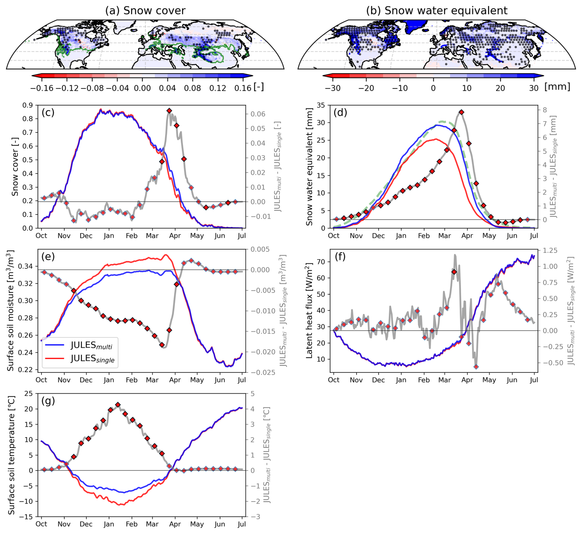
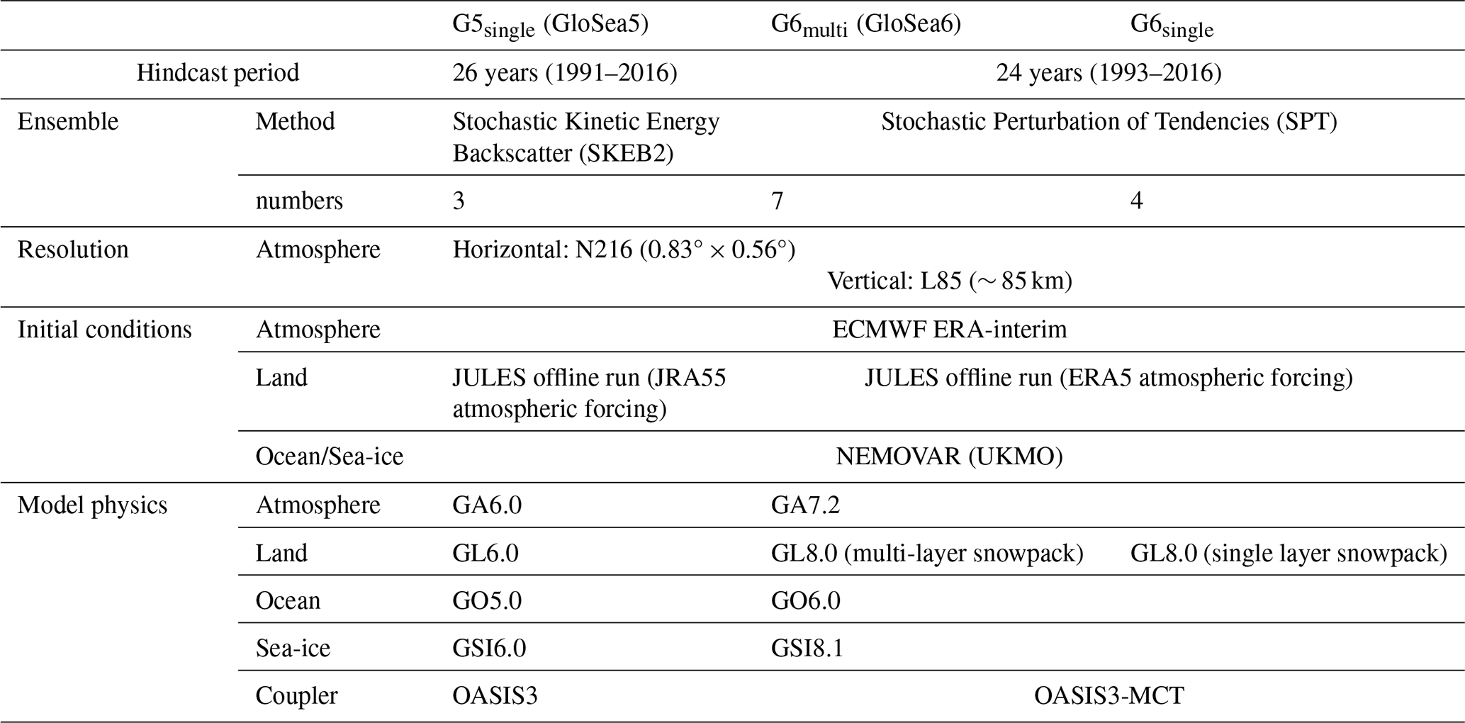
Figure 1 Spatial patterns of climatological difference (JULES_multi−JULES_single) of (a) snow cover and (b) snow water equivalent, averaged over March–April for the 22-year (2001–2022), where the dotted area indicates the difference is statistically significant at a 95 % confidence level after FDR control across the grid. The green contour line in (a) indicates a snow cover of 0.15 from JULES_multi experiment. Climatological seasonal cycle of 24-year averaged (a) snow cover, (b) snow water equivalent, (c) surface soil moisture, (d) latent heat flux, and (e) surface soil temperature simulated by JULES_single (red) and JULES_multi (blue) over the Eurasian continent (0–130° E, 45–55° N). To denote the response of land variables to the snow physics scheme, the green dashed line in (d) denotes JRA-3Q snow water equivalent grey solid lines in (c)–(g) display the difference between JULES_multi and JULES_single throughout the snow accumulation and melting seasons. In (c)–(g), the black outlines on the red markers indicate when the climatological difference within the 11 d window on each calendar date is statistically significant at a 95 % confidence level.

Figure 2 Climatological seasonal cycle of 24-year (1993–2016) averaged (a) snow water equivalent, (b) surface soil moisture, (c) surface soil temperature, (d) surface air temperature, (e) surface albedo, (f) net radiation, (g) latent heat flux, (h) sensible heat flux and (i) precipitation simulated by G6_single (red) and G6_multi (GloSea6, blue) over the Eurasian continent (0–130° E, 45–55° N). 100 d forecast lines fade at increasing lead forecasts and coloured marks indicate initial states on the first day of each month, where 21 d running averaged time series are not displayed with coloured marks (surface soil temperature shows 60 d forecast due to data availability), while 180 d forecast lines are denoted on 1 March initiated runs. Grey lines in (a)–(i) display the climatological difference (solid: G6_multi–G5_single, dashed: G6_multi–G6_single) throughout the snow accumulation and melting seasons. The red markers edged in black indicate that the difference of G6_multi–G6_single within the 11 d window on each calendar date is statistically significant at a 95 % confidence level. (j) Lead-lag correlation coefficient for the daily time series of the difference between G6_multi and G6_single for the coupling of SSM-LH (red) and LH-PR (blue) with 120 d forecast initiated at each year on 1 March. A positive lagged day indicates that SSM and LH leads LH and PR, respectively, and negative is vice versa.

3.1 Soil moisture memory

To evaluate the SM persistence simulated in the model, the autocorrelation-based SMM is employed. First, assuming that the evolution of the daily SM time series follows a first-order Markov process (Vinnikov and Yeserkepova, 1991), the decay frequency (f) of SM can be defined by a function of SM autocorrelation (AR) at lag day (τ) (Dirmeyer et al., 2016; Seo and Dirmeyer, 2022a). Its formulation is followed as:

$$\mathrm{AR}\left(\mathit{\tau }\right)=\exp (-f\mathit{\tau })$$

The SMM is defined with an e-folding decay time, at which the autocorrelation of SM drops to $\mathrm{1}/e$. By a linear fitting of ln[AR(τ)], the memory is calculated as the value of τ, when the linear extrapolation between ln[AR(τ=1)] and ln[AR(τ=2)] is intersected to ln$\left[\mathrm{AR}\left(\mathit{\tau }\right)\right]=-\mathrm{1}$. Since the SM behavior is not perfectly fitted on the first-order Markov process, the displacement of the extrapolated linear fit at τ=0 is defined with the measurement error mostly attributed to random errors (Robock et al., 1995). To measure the SMM under the assumption that there is no measurement error, the extrapolated linear fit is shifted to intersect origin point and the intersected τ value between the shifted linear fit and ln$\left[\mathrm{AR}\left(\mathit{\tau }\right)\right]=-\mathrm{1}$ is the corrected SMM. Time-filtered ESA CCI and modeled SM products exhibit the marginal measurement error (Seo and Dirmeyer, 2022a), so that this study focuses on the improvement in the representation of the corrected SMM in the model simulations. The autocorrelation is calculated by concatenated time series of daily SM over JJA (June–August) of 17 years (2000–2016) with modelled and time-filtered satellite SM time series. In the calculation of the SMM in both seasonal forecast systems, to minimize the impact of systematic forecast drift, the JJA SM time series for each year are constructed by concatenating 1-month lead forecasts for each respective month, specifically June from the 1 May initialization, July from 1 June, and August from 1 July. The time series for each year are further concatenated to produce the 17-year JJA SM time series. The SMM is calculated in each ensemble forecast and represented by the median of the ensemble values. Additionally, the statistical significance of SMM biases in both simulations and their difference between GloSea5 and GloSea6 is tested using a Monte Carlo approach. The probability of a significant SMM is estimated by random sampling, where randomly selected yearly JJA SM time series (92 samples) are used to create all-year JJA time series, repeatedly, to generate 100 samples in observational and modelled datasets. For testing the statistical significance of the modeled SMM biases, randomly calculated SMMs from time-filtered CCI, ERA5-Land, and GLEAM products are used to generate 300 observational samples (3 products × 100 random SMMs), which are compared to 300 and 700 random samples from GloSea5 (3 ensembles × 100 random SMMs) and GloSea6 (7 ensembles × 100 random SMMs), respectively, using a Student's t-test. The statistical significance of the SMM difference between the two model simulations is also tested with the randomly calculated 300 and 700 SMM samples.

3.2 Granger causality in evaporation-precipitation feedback

To characterize the causality of land-atmosphere interactions, this study adopts the Granger causality test, that originates from the field of econometrics (Granger, 1969; Salvucci et al., 2002). This is a statistical principle to identify the potential dependence of a target variable on source variable beyond any persistence (memory) inherent in the target variable. To explore the quantitative understanding of evaporation-precipitation feedback, this study investigates the causality between a source variable (SV: hypothesized to trigger a feedback) and target variable (TV: responding to the feedback), where the statistical time-lagged response of the land-atmosphere feedback is applied by setting a 1 d time lag in the time series of TV compared with SV. This is formulated as:

$$\begin{array}{}\text{(1)}& F\left({\mathrm{TV}}_t\mathrm{|}{\mathrm{\Omega }}_{t-\mathrm{1}}\right)\ne F({\mathrm{TV}}_t\mathrm{|}{\mathrm{\Omega }}_{t-\mathrm{1}}-{\mathrm{SV}}_{t-\mathrm{1}})\end{array}$$

where F is the conditional distribution of TV on a given day, Ω_t−1 denotes the set of all knowledge available at t−1 time, and ${\mathrm{\Omega }}_{t-\mathrm{1}}-{\mathrm{SV}}_{t-\mathrm{1}}$ represents all knowledge except SV. We employ evaporative fraction $(\mathrm{EF}=LE/(H+LE\left)\right)$ and precipitation (PR) in each role to identify the response of precipitation variability to the land surface flux partitioning (GC(PR_t|EF_t−1)) and vice versa (GC(EF_t|PR_t−1)). As the null hypothesis equates that SV does not affect TV, the rejected probability of the null hypothesis (1−p) is calculated to intuitively understand the causality. Nevertheless, as Granger causality only tests for predictive precedence, the results may reflect statistical associations of predictive precedence due to shared external drivers and should not be interpreted as definitive physical causation between both variables. Specifically, shared external atmospheric drivers can influence both evaporation and precipitation, potentially confounding the identified causal links. The analysis is conducted using 24-year forecast runs initialized on 1 March for each forecast experiment, and to compare to the causality in observations, EF and PR are taken from the GLEAM and MSWEP datasets, respectively.

3.3 Methodology to characterize land coupling

This study evaluates model performance in the simulation of land coupling processes in fully coupled forecast models. Land-atmosphere interaction is controlled by land surface energy and water exchanges. Depending on their relative dominance, water- and energy-limited regimes are categorized, where the flux partitioning between sensible and latent heat flux is controlled by the availability and variability of SM or by net radiation mainly dictated by the atmosphere, respectively. They are separated by a critical value of SM at each location; the dry and wet side of the critical value exhibits water- and energy-limited coupling processes, respectively. Corresponding to the dominant response of the partitioning of land heat fluxes attributed to either the land state or the atmosphere, the direction of land-atmosphere coupling is land-to-atmosphere or atmosphere-to-land, respectively (see Fig. 2 in Seo et al., 2024).

To quantify the strength of land-atmosphere coupling based on either the water- or energy-budget predominance, this study compares the temporal correlation of latent heat flux (the key variable linking water and energy budgets) with the surface SM [R(SSMLH)] and net radiation [R(R_nLH)], respectively. While both latent heat flux and net radiation are physically linked (as latent heat is energetically constrained by net radiation), the correlation between them helps infer the extent to which surface fluxes follow the available energy signal. However, it is important to note that R(R_nLH) is not independent of the water budget, and high correlation values may still occur in water-limited regimes if increased net radiation results in greater latent heat flux under sufficient SM. Therefore, these metrics are interpreted as complementary diagnostics, with R(SSMLH) highlighting land-state sensitivity and R(R_nLH) indicating energy control, rather than mutually exclusive regime indicators. While direct differences between G6_multi and G6_single isolate the mean state impact, these metrics provide process-based validation by assessing the model's fidelity in simulating the underlying processes. The analysis is conducted using MJJA time series of 24-year forecast runs initialized on 1 March for each forecast experiment and ensemble member. The results exhibit a negligible discrepancy with the analysis of the JJA time series (not shown), which accounts for forecast drift and seasonality during the transitional period.

4 Results

4.1 Seasonality of land surface variables

To assess the impact of multi-layer snowpack scheme on the simulation of snow freezing and melting processes, this study compares the representation of the seasonal cycle of land surface variables between JULES_single and JULES_multi. In both JULES offline experiments, the seasonal cycle of snow cover peaks in late December over the mid-latitudes of Eurasia (Fig. 1c), while SWE reaches its peak approximately two months later (Fig. 1d). When the multi-layer snow scheme is applied in JULES_multi, the insulating effect of the land surface delays the onset of snowmelt, resulting in higher values of both snow cover and SWE during early spring season (March–April), which more closely resemble the observed seasonal cycle of SWE. The multi-layer snow scheme leads to an expansion of snow-covered areas, shifting the springtime snow frontal zone northward to around 40° N and significantly increasing the amount of snow within the snow-covered regions (Fig. 1a, b). The effect of the multi-layer snow scheme on soil and air temperatures depends on the snow accumulation, snow peak, and snow melting seasons. The air temperature response will be specifically addressed in Fig. 2, which is based on the coupled model simulation, since the offline model is forced by near-surface atmospheric variables, including surface air temperature.

The snowpack plays the role of limiting the transfer of heat between air and soil due to the enhanced insulation. Therefore, the multi-layer snow scheme provides a stronger insulating effect, simulating significantly warmer soil temperature from snow cover onset through March, when air is colder than the land surface (Fig. 1g). The warmer soil temperature in JULES_multi (Fig. 1g), induced by the snow insulation effect, increases the fraction of unfrozen SM. Unlike soil ice, liquid water in the soil remains mobile, contributing to subsurface runoff and potentially evaporation, resulting in drier soil (Fig. 1e). JULES_multi simulates abundant snow variables in March, accompanied by an increase in latent heat flux (Fig. 1f). Following the largest difference in snow between the two JULES runs in March, the SM difference begins to decrease, subsequently resulting in wetter soil conditions in the JULES experiment during April. This, in turn, leads to enhanced latent heat flux in April, but the differences for land surface variables in the offline experiments is insignificant after April.

Furthermore, to explore the model performance in simulating snow freezing and melting processes in fully coupled forecast systems, we also compare the seasonal cycle of the land variables for G5_single, G6_single, and G6_multi. Specifically, the effect of a multi-layer snowpack scheme during October–February and March–August is primarily compared to G6_multi–G5_single and G6_multi–G6_single, respectively. Although the land initial conditions are generated by different atmospheric forcing in GloSea5 (G5_single) and GloSea6 (G6_single and G6_multi), an analysis of 1 d forecast fields, which serve as a robust proxy for the initial land state due to their slow evolution, confirms that the difference in initial snow amount is statistically insignificant (Fig. S2). Differences in winter precipitation between both models may lead to variations in snow accumulation; however, although GloSea6 generally simulates slightly higher precipitation, the magnitude of this difference is negligible compared to the difference in snow water equivalent (not shown). Therefore, the impact of precipitation on snow accumulation is not considered in this study. GloSea6 simulates the seasonal cycle of snow freezing process over the Eurasian continent (Fig. 2a) similarly to the results from the JULES offline run. Given that the primary source of energy for snowmelt is the atmosphere, snow melting process is tied to the variation of surface air temperature (cf. Fig. 2d). Snow dissipates 1–2 weeks earlier in the early summer when a single layer snowpack is adopted in G5_single and G6_single. For instance, G6_single and G6_multi consistently initiate a snow peak in March and are initiated with similar snow conditions in that month, but the snow in G6_single disappears before June while it persists until early June in G6_multi.

Although similar SM states are initialized in GloSea5 and GloSea6 for the entire analysis period, G5_single shows a model forecast drift in the wet direction from October to March (Fig. 2b). The differences in SM initial conditions in October and November are attributed to differences in the atmospheric forcing used to drive the LSM during the generation of land surface initial states. Because the snowpack serves as a barrier to energy and water exchange between the land and the atmosphere, in the single layer snowpack, the early onset of evaporation manifests the physical process of drying out SM during snow melting season. Wetter soil moisture is simulated in G5_single during October, when snow cover is minimal, which is attributed to a positive precipitation bias (not shown). Thus, the implementation of the multi-layer snowpack results in the climatologically drier and wetter SM, respectively, preceding (November–March) and following (April–June) the onset of snowmelt. However, in the JULES offline simulations, the implementation of the multi-layer snowpack results in wetter SM only during April, with no significant differences persisting into the summer. This suggests that the influence of advanced snow physics becomes more pronounced when the land is coupled with the atmosphere, allowing its effects to extend into the summer season. The drier SM climatology of G5_single compared to G6_single indicates that the realization of the model climatology is not only due to the advancement of snow physics, but also to other updates in GloSea6.

For the radiation balance, net radiation during the snow freezing season can decrease due to enhanced upward longwave radiation driven by surface warming, despite a concurrent increase associated with reduced surface albedo. These two opposing effects tend to offset each other, resulting in minimal differences in net radiation during this period (Fig. 2f). However, during the snow peak season (February–March), the surface albedo effect becomes more dominant (Fig. 2e), leading to an increase in net radiation. In late spring (April–May), when differences in snow variables become more pronounced, surface albedo increases and surface cooling occurs (Fig. 2d), which plays a role opposite to that observed in winter. During this period, the stronger influence of increased surface albedo leads to a decrease in net radiation.

In the coupled model simulations, the effect of the multi-layer snow scheme on soil temperature during the snow-covered is consistent with the results from the JULES offline simulations, but the soil temperature cooling is observed during the summer season (Fig. 2c), which is responsible for surface air temperature. For the surface air temperature, G6_multi is colder during the snow freezing season due to limited energy transfer from the cold air to the snow surface (Fig. 2d). During the two-month snow peak period from mid-January, G6_multi simulates higher air temperature due to warmer ground, resulting in less cooling from the soil. The air temperature cooling observed from mid-March is associated with decreased net radiation due to enhanced surface albedo. The continuous cooling after diminishing the snow effect can be explained by evaporative cooling driven by increased latent heat flux (Fig. 2g). In other words, the radiation is primarily balanced by latent heat flux in G6_multi due to abundant SM, but sensible heat flux decreases due to air temperature reductions (Fig. 2h).

Additionally, the increased latent heat flux supplies water to the boundary layer, triggering precipitation and thereby increasing the mean climatology of precipitation (Fig. 2i). While the additional 1 W m⁻² of latent heat flux appears marginal, it is critical to consider the accumulated effect over the seasonal forecast period. A small anomaly can be significant when persistent, in the context of land-atmosphere coupling. For instance, a persistent difference of 1 W m⁻² in latent heat flux over one month translates to a cumulative change of ∼ 1 mm in the water budget. Such an alteration in the regional water and energy budget is physically meaningful and can serve as a non-negligible source of memory and predictability in precipitation. To illustrate the physical sequence between land surface variables by the realization of snow physics, the lead-lag correlation of major water budget variables is compared between G6_single and G6_multi (Fig. 2j). The results show the hydrological chain of SSM → LH → PR with a positive correlation among variables in each segment, characterized by a lead-lag time of approximately one week. In other words, the increased soil moisture in mid-latitude regions likely increases precipitation based on positive evapotranspiration-precipitation feedback. The positive feedback is typically observed in numerical forecast systems, including HadGEM2-AO (atmosphere-land only coupled forecast model of GloSea5), in contrast to observation-based analyses, which indicate a negative coupling between SM and precipitation (Taylor et al., 2012).

The substantial difference between G5_single and G6_single confirms that updates other than the snow scheme contribute significantly to the climatological mean change in the simulation of land surface variables. However, the core finding of this study is the demonstration that the implementation of the multi-layer snow scheme yields a statistically significant and physically consistent impact that is independent of these other updates.

4.2 Evaluation of model climatological error and bias over the Northern Hemisphere

Although soil moisture has historically not been a verifiable quantity in weather forecast models (Koster et al., 2009), the adoption of soil moisture data assimilation makes soil moisture a variable for validation (Seo et al., 2021). To examine the representation of surface SM when implementing multi-layer snowpack scheme, this study compares the climatological mean of land variables relevant to water budget between G6_single and G6_multi (Fig. 3). The difference in SM simulation for May–August is large poleward of 40° N (Fig. 3f), which is pronounced over the snow frontal region, suggesting that the difference is related to the additional snow insulating effect in the G6_multi LSM. The difference in snow variables (i.e., SWE and surface albedo) for the spring season shows that the multi-layer snowpack significantly prolongs the snow properties over snow covered regions (Fig. 3d, e).

Figure 3 Spatial distribution of climatological (a) snow water equivalent (March–May), (b) surface albedo (March–May), (c) surface soil moisture (May–August) from GloSea6 (G6_multi) initiated on 1 March of 1993–2016. (d, e, f) Their difference maps compared to G6_single, where the dotted area indicates the difference is statistically significant at a 95 % confidence level after FDR control across the grid.

Since SMM is a key factor in the subseasonal forecasting because of its persistence over a few weeks, model fidelity of SMM is crucial for forecast skill. Because memory is shortened by occurrences of precipitation, it is prolonged where the climate is relatively dry. For instance, SM persistence is relatively short over East Asia where the monsoon flow throughout the summer season leads to an increasing likelihood of rainfall, accompanying wet soil. The spatial patterns of SMM from ESACCI_adj, ERA5-Land, and GLEAM are similar (Fig. 4a, b, c), but ESACCI_adj is noisy at high-latitudes because SM dynamics are not perceived by the satellite when the surface is frozen. The NH averaged values of SMM from ESACCI_adj, ERA5-Land, and GLEAM are 8.6, 8.5, and 11.1 d. The spatial distribution of SMM determined from the observational products is reliably simulated over the NH in G6_single and G6_multi. Improvements in SMM spatial agreement are shown in G6_multi (Fig. 4d, e), where the spatial correlation of the SMM with GLEAM is increased. In contrast, the SMM in G6_multi is increased when the soil wetness becomes wetter even though its positive bias is observed in G6_single compared to the SMM from GLEAM. When the soil becomes wet due to the late onset of snow melting, the SM decay in response to rainfall is slow, thereby significantly increasing the SMM in mid-latitude regions (Fig. 4f).

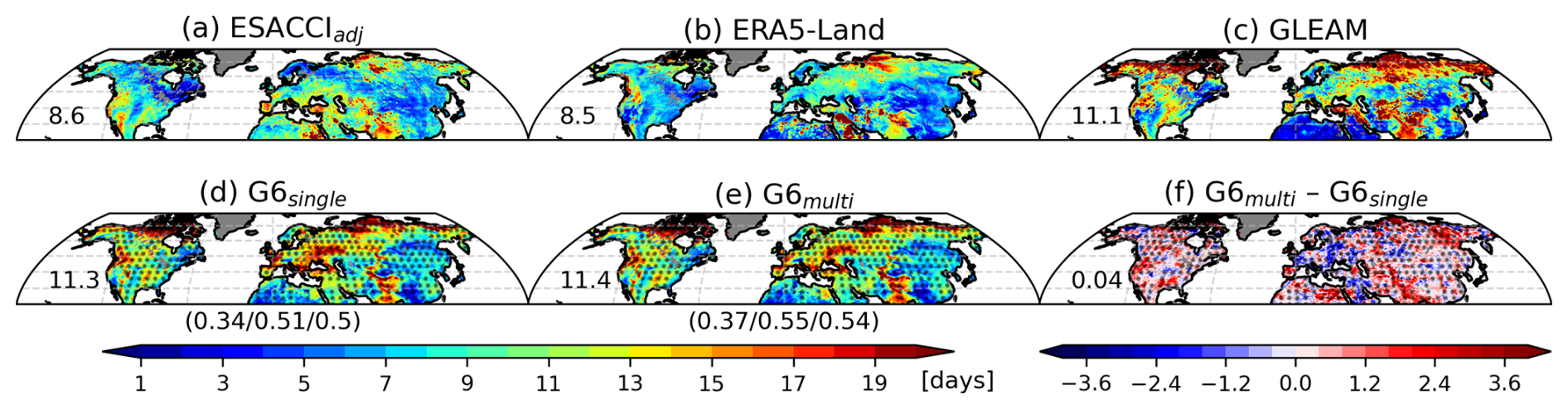
Figure 4 Surface SMM from (a) ESACCI_adj, (b) ERA5-Land, (c) GLEAM, (d) G6_single, (e) G6_multi, and (f) the difference between G6_multi and G6_single. NH mean values are denoted in the middle-left in each panel. The bracketed values indicate the spatial correlation of the modelled soil moisture memory compared to ESACCI_adj (left), ERA5-Land (middle), and GLEAM (right). Dotted areas represent statistical significance of SMM difference between models and observations (d–e) and between models (f) at the 99 % confidence level from a Monte Carlo method.

Features of the surface air temperature simulation in G6_multi during the NH summer season include reduced positive biases in both daily mean and sub-daily timescales over snow frontal regions (Fig. 5), which can be explained by the updated land surface physics, including changes in snow and soil processes. G6_multi simulates colder temperatures over the mid-latitudes, compared to G6_single (Fig. 5c). To identify the impact of a major modification in the LSM on temperature simulation, the assessment of Tmean is decomposed into the Tmax and Tmin. Both daytime and nighttime temperatures are analysed in addition to daily mean temperature to assess whether temperature changes associated with land surface processes occur preferentially during the day or night. Since many coupled land-atmosphere processes are typically more active during the daytime due to greater available energy (net radiation), sub-daily analysis is essential for realistically capturing their effects (Yin et al., 2023; Seo and Dirmeyer, 2022b). Furthermore, relying solely on Tmean can be misleading, as it conflates errors in maximum and minimum temperatures, and thus does not necessarily reflect an overall improvement in model performance (Seo et al., 2024). The effect of the multi-layer snow scheme on forecasting temperature is primarily surface cooling over snow frontal areas throughout the entire day (Fig. 5c), even though the temperature response is more sensitive during the daytime when land-atmosphere interactions are most active (Fig. 5f, i). This is because there is a larger latent heat flux during the daytime, resulting in a larger evaporative cooling.

Figure 5 Spatial distribution of daily mean (upper row; a–c), maximum (second row; d–f), minimum (third row; g–i) surface air temperature, and precipitation (lower row; j–l) bias during boreal summer season (June–August) in G6_single (first column), G6_multi (second column), and the difference between both models (last column), where the dotted areas indicate statistical significance at a 95 % confidence level after FDR control across the grid. In each panel, grey horizontal lines isolate a mid-latitude area (40–55° N) and area averaged values is denoted within grey shaded box.

Model performance in simulating precipitation is also evaluated in G6_single and G6_multi. Both models show an overestimation over East Asia and high-latitude regions and an underestimation over the central US and western and central Eurasia (Fig. 5j, k). While the positive bias is amplified or maintained in areas that have wet biases in G6_single, the area noted by the negative bias is decreased (Fig. 5j, l). The increased precipitation in G6_multi over the mid-latitude regions (Fig. 5l) is explained by the abundant SM from snow melting process under positive evapotranspiration-precipitation feedback (cf., Fig. 8).

To demonstrate the impact of land-atmosphere interactions on the model's ability to simulate precipitation, this study assesses the time-lagged Granger causality between EF and PR. The observed causality generally represents that the null hypothesis is rejected (1−p value > 0.05) regardless of feedback direction, indicating evaporation-precipitation feedback over mid-latitude regions (Fig. 6a, b). The causal probability in the direction from PR to EF, GC(EF_t|PR_t−1), is generally pronounced over the globe, with particularly strong feedback over the areas where precipitation variability is primarily attributed to large-scale atmospheric circulations (e.g., South and East Asia), while the dominance of GC(PR_t|EF_t−1) is strongest over western North America (Fig. 6c). However, G6_single shows the overall overestimation in both casual directions between EF and PR (Fig. 6d, e), whereas a negative bias in GC(EF_t|PR_t−1) is shown over the high-latitudes of Eurasia. The difference map of GC(EF_t|PR_t−1) and GC(PR_t|EF_t−1) simulated in G6_single shows a negative bias over western North America and northern Eurasia due to overestimated GC(PR_t | EF_t−1) and underestimated GC(EF_t | PR_t−1) (Fig. 6f), respectively. The biases of the evaporation-precipitation feedback in both casual directions are reduced in G6_multi (Fig. 6g, h).

Figure 6 Spatial distribution of 1 d lagged Granger causality (1−p value) with evaporative fraction and precipitation. The observed causalities (a) GC(EF_t | PR_t−1), (b) GC(PR_t | EF_t−1), and (c) their difference in which blue and red color indicates the dominance of feedback direction in GC(EF_t | PR_t−1) and GC(PR_t | EF_t−1), respectively. The model biases of G6_single compared to observations for the causality in (d) GC(EF_t | PR_t−1), (e) GC(PR_t | EF_t−1), and (f) the difference between GC(EF_t | PR_t−1) and GC(PR_t | EF_t−1) in G6_single. The difference maps of (g) GC(EF_t | PR_t−1) and (h) GC(PR_t | EF_t−1) between G6_single and G6_multi and (i) the difference between GC(EF_t | PR_t−1) and GC(PR_t | EF_t−1) in G6_multi.

4.3 Representation of land coupling processes

The exchanges at the land surface are constrained by the water and energy balance equations, and the strength of water- versus energy-limited processes is quantified by the temporal correlation coefficient of latent heat flux to surface SM or net radiation, respectively, as described in Sect. 3.3. The spatial pattern of the GLEAM land coupling is similar to the distribution of the SM climatology, such that water-limited processes are pronounced over climatologically dry areas and vice versa. The classification of the land coupling results from the synthetization of the spatial pattern of R(SSMLH) (Fig. 7a) and R(R_nLH) (Fig. 7b), recognizing that both variables are interconnected through the surface energy and water budgets. Since latent heat flux is influenced by both SM availability and incoming radiation, positive correlations in both R(SSMLH) and R(R_nLH) can occur simultaneously, especially in transitional regimes (cf., Denissen et al., 2020). This overlap does not contradict the diagnostic framework but reflects the continuum of land-atmosphere coupling conditions. For instance, the spatial distribution of R(SSMLH) and R(R_nLH) is a zonal dipole structure over CONUS but is meridionally banded over Eurasia. Note that R(SSMLH) and R(R_nLH) are not mutually exclusive and may both be positive in transitional regimes.

Figure 7 Spatial distribution of R(SSMLH) (left column; water-limited coupling) and R(R_nLH) (middle column; energy-limited coupling) in (a, b) GLEAM, (c, d) model biases of G6_single compared to observations, and (e, f) differences between G6_single and G6_multi, where grey horizontal lines in each panel separate to mid- (20–55° N) and high-latitude (55–80° N) areas and area averaged values is denoted within grey shaded box. The dotted areas in (c)–(f) indicate statistical significance at a 95 % confidence level after FDR control across the grid. (g) Boxplot of the squared spatial pattern correlation coefficient as a measure of the spatial agreement of R(SSMLH) (SC_w) and R(R_nLH) (SC_e) in G6_single (red) and G6_multi (orange) over the northern hemisphere against GLEAMv4.2a. Boxes show the median and interquartile range (IQR: 25th and 75th percentiles), and whiskers represent ±0.5IQR from the 25th and 75th percentiles, respectively, and dotted circles indicate the sampled average. In the rightmost column, SC_w×SC_e quantifies the coherency of water- and energy-limited processes in both models.

G6_single exhibits an overestimation of R(SSMLH) over the mid-latitude regions, which results in the expansion of water-limited areas and the degradation of the spatial characteristics in the observation, while the negative bias is particularly evident over high-latitude regions (Fig. 7c). G6_multi represents a similar bias pattern to the G6_single, whereas the positive and negative biases in the high-latitude areas are directionally improved (Fig. 7e). G6_single reveals a negative bias in the energy-limited coupling, especially over the high-latitude areas (Fig. 7d), but G6_multi significantly promotes the energy-limited coupling strength, which mitigates the negative bias of R(R_n,LH) (Fig. 7f). The delayed snowmelt simulated in G6_multi leads to increased SM during the warm season, which likely contributes to enhanced evaporative partitioning. While this may weaken the sensitivity of latent heat flux to SM (i.e., reducing R(SSMLH)) and strengthen the relationship with net radiation (i.e., increasing R(R_n,LH)), we acknowledge that this interpretation is subject to direct evidence of causal feedback by snow-related land surface processes. Furthermore, the pattern agreement between the land coupling features simulated by both forecast models and the observation is measured by the spatial correlation coefficient of R(SSMLH) (SC_w) and R(R_nLH) (SC_e) (Fig. 7g). While G6_single and G6_multi show superior performance in capturing the observed pattern in energy-limited processes, the multi-layer snowpack scheme assists in increasing spatial consistency in both land coupling processes along with the improvements in modelled mean bias. Therefore, constructing the squared spatial correlation with SC_w×SC_e, which synthesizes the model performance of the land coupling processes in terms of the water- and energy-limited coupling, shows higher values in G6_multi.

5 Summary and Conclusions

Some land surface models have employed a single layer snow scheme that treats snow as a modification of the top-soil layer. While effective for very thin snow cover, such a composite scheme struggles to simulate the true insulating effect of the snowpack because it lacks the internal thermal gradient necessary to buffer energy transport between the land and atmosphere in deeper snow. Therefore, the benefits of the multi-layer scheme demonstrated in this study should be interpreted as an improvement over this specific single-layer formulation.

Figure 8 Schematic of the impact of the multi-layer snow scheme on the seasonal forecast system on the evolution of the land surface from winter through the following summer.

This study primarily investigates the impact of implementing a multi-layer snow scheme on the climatological bias in both LSM offline simulations and fully coupled forecast systems. Two sets of LSM experiments are conducted using JULES version 5.6, the land surface component of GloSea6 – one employing the single layer snow scheme and the other incorporating the multi-layer snowpack scheme. The multi-layer configuration yields a more realistic simulation of snow seasonality compared to reanalysis data. Notably, it captures the onset of snowmelt more accurately by better representing the insulating effect of snow.

To elucidate the role of snow insulating effect in coupled forecast system, we analyse GloSea global retrospective seasonal forecasts over 24 years (1993–2016) from two model versions: GloSea6 (G6_multi), which implements the multi-layer scheme, and GloSea5 (G5_single), which retains a single-layer scheme. Furthermore, we have conducted an additional experiment that implements a single layer snowpack scheme in GloSea6, referred to as G6_single, to isolate solely the effects of the advancement of snow physics. Improvements in the model simulations appearing in areas with high snow variability can be understood as the effect of the multi-layer snow scheme. The improved snow physics with a multi-layer snowpack better captures the observed snow dissipation season (Fig. 2a) and influences land and near-surface variables throughout the snow accumulation and melting seasons. The near-surface warming and cooling caused by the insulating effect of the snowpack during the snow peak and melting seasons (Fig. 2d) results in a late onset of snow melt and wetter SM during the subsequent summer season, particularly in mid- to high-latitude regions (Figs. 2b and 3f). The changes in land surface processes also affects land surface characteristics, e.g. SM memory is generally increased, which improves spatial agreement compared to the observational analysis (Fig. 4). Moreover, the greater SM from the advanced snow physics leads to a decrease in surface air temperature with evaporative cooling throughout the entire day (Fig. 5) and increases the likelihood of precipitation explained by evapotranspiration-precipitation feedback (Fig. 6). However, the effect of improved snow physics in the fully coupled model is not consistent with the result from the LSM offline experiments, particularly after snowmelt, because the impacts of realized snow behaviour become more pronounced when the atmosphere interacts with the land.

The spatial distribution of the land coupling reflects the underlying SM climatology, with the majority of water- and energy-limited coupling corresponding to relatively dry and wet soils, respectively (Fig. 7). Evaluating these regimes is essential for understanding model behaviours associated with land-atmosphere coupling processes. Comparing the land coupling processes simulated by G6_single and G6_multi, the increased SM in G6_multi alters the coupling characteristics, weakening water-limited coupling while enhancing energy-limited processes (Fig. 7e, f). Although both models still tend to overestimate and underestimate water- and energy-limited coupling over mid- and high-latitude regions, respectively, the multi-layer snow scheme reduces this bias. The increased SM due to the late onset of snowmelt restricts water-limited coupling, evidenced by increased R(R_nLH) and decreased R(SSMLH). This shift demonstrates a robust improvement in the underlying land-atmosphere coupling processes, leading to a better simulation of near-surface atmospheric variables (namely temperature and precipitation).

Since realistic snow states influence the water and energy budgets not only in winter but also in spring and summer (Fig. 8), the realization of snow characteristics should be a priority in the process of developing a model. Importantly, modifying land surface schemes to improve warm-season processes without addressing snow dynamics may lead to increased errors – even if snow is realistically simulated. It is also worth noting that improvements in climatology do not directly translate to enhanced forecast skill; in this study, improvements in temperature and precipitation skill in GloSea6 are primarily attributed to the larger ensemble size (Figs. S3 and S4). In conclusion, the implementation of a multi-layer snow scheme is essential for realistically simulating land surface processes in S2S dynamical forecast systems. From a climate perspective, as global warming increases both the variability and uncertainty in modelled snow conditions, reliable future climate projections will depend on the selective use of models that are able to simulate realistic snow characteristics.