The Western United States Large Forest-Fire Stochastic Simulator (WULFFSS) 1.0: a monthly gridded forest-fire model using interpretable statistics

We developed the WULFFSS, a stochastic monthly gridded forest-fire model for the western United States (US). Operating at 12 km resolution, WULFFSS calculates monthly probabilities of fires that burn at least 100 ha of forest area as well as the forest area burned per fire. The model is forced by variables related to vegetation, topographic, anthropogenic, and climate factors, organized into three indices representing spatial, annual-cycle, and lower frequency temporal domains. These indices can interact, so variables promoting fire in one domain amplify fire-promoting effects in another. Fire probability and size models use multiple logistic and linear regression, respectively, and can be easily updated as new data or ideas emerge. During its training period of 1985–2024, WULFFSS captures 71 % and 86 % of observed interannual variability in western US forest-fire frequency and area, respectively. It reproduces regional differences in seasonal timing, frequencies, and sizes of fires, and performs well in cross-validation exercises that test the model's accuracy in years or regions not considered during model training. While lacking fine-scale fire dynamics, use of classic statistics promotes interpretability and efficient ensemble generation. Designed to run within a vegetation ecosystem model, bidirectional feedbacks between vegetation and fire can identify how ecosystem changes have altered or will alter fire-climate relationships across the western US. The model's predictive power should improve with increasingly accurate and extensive observational data, and its approach can be extended to other regions. Here we provide a thorough description of the WULFFSS model, including the motivation underlying its development, caveats to our approach, and areas for future improvement.

1 Introduction

In the western United States (US), the annual wildfire area increased by approximately 250 % from 1985–2024, largely because annual forest-fire extent increased 10-fold (902 %) during this time (Fig. 1a). These rapid increases in annual area burned over the last few decades occurred despite consistent efforts to suppress wildfire (Fig. 1b), signifying a break from the ease with which fires were contained through most of the 20th century. Importantly, the frequency of western US forest fires has not increased in recent decades (Syphard et al., 2025), so it is the growing sizes of fires rather than their numbers that are responsible for the rapid increases in area burned (Juang et al., 2022). Severe, stand-replacing forest fires also appear to have been more prevalent in recent decades than in previous centuries (Parks and Abatzoglou, 2020; Hagmann et al., 2021; Higuera et al., 2021; Parks et al., 2023; Williams et al., 2023). Thus, even though western US fires are still less common than during pre-European centuries (Parks et al., 2025), the rapid recent increase in fire activity has often not been ecologically restorative (Coop et al., 2020). Further, carbon emissions from increasingly large and severe fires work against carbon-neutrality targets for climate change mitigation (Anderegg et al., 2022, 2024; Jones et al., 2024). Growing sizes and spread rates (Balch et al., 2024) of severe forest fires in the western US have also combined with growing human populations in fire-prone areas (Radeloff et al., 2023) to increasingly put people and property in harm's way (Higuera et al., 2023), including via air pollution far from the flames themselves (Burke et al., 2023). Continued growth in forest-fire sizes and severities may also alter mountain hydrology, with cascading impacts on water resources and flood risk (Kampf et al., 2022; Williams et al., 2022). These trends motivate improved understanding of, and capability to model, past and future changes to western US forest-fire activity.

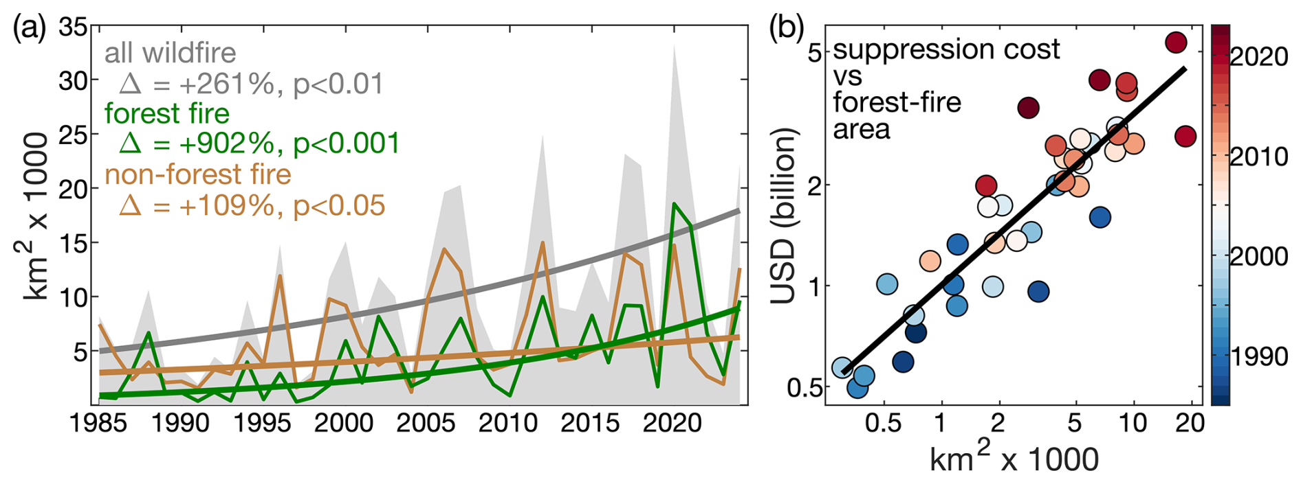
Figure 1 Annual western US wildfire extent and suppression expenditures. (a) Time series of annual western US (grey) total wildfire area, (green) forest area burned, and (brown) non-forest area burned from 1985–2024. Bold lines show the Theil-Sen trends in the logarithm of area burned. Delta (Δ) values indicate the relative change from the first to last year of each trend and p-values indicate trend significance assessed with one-tailed block (2 year) bootstrap. (b) Scatterplot of annual federal fire suppression cost versus forest-fire area (colors correspond to year) from 1985–2023 (suppression cost unavailable for 2024). Federal suppression costs from https://www.nifc.gov/fire-information/statistics/suppression-costs (last access: 30 December 2025) and inflation-adjusted to 2024 US dollars. Fire dataset described in Sect. 3.1.

Drying and warming have been primary drivers of the increase in western US forest area burned in recent decades (Westerling et al., 2006; Abatzoglou and Williams, 2016; Holden et al., 2018; Williams et al., 2019; Brown et al., 2023). Precipitation declines from the early 1980s to the early 2020s were promoted by trends toward the cool states of the El Niño-Southern Oscillation and Pacific Decadal Variability (Lehner et al., 2018), which were probably mostly due to natural climate variability but potentially also promoted by anthropogenic forcing (Hwang et al., 2024; Jiang et al., 2024). The linkage between anthropogenic forcing and warming is clearer and likely to continue (Vose et al., 2017). Warming primarily reduces forest fuel moisture by enhancing the atmosphere's evaporative demand, melting snow earlier in the year, and extending the season of vegetation water use. Temperature drives atmospheric moisture demand through its exponential impact on the vapor pressure deficit (VPD), and this variable is strongly correlated with annual forest-fire area in the western US (He et al., 2025) (Fig. 2, left side). Fuel moisture and wildfire activity are also critically affected by other climate variables, including precipitation total, precipitation frequency, and dry windiness (Abatzoglou and Kolden, 2013; Williams et al., 2015; Holden et al., 2018; Brey et al., 2021). Considering a number of methods to quantify fuel aridity, Abatzoglou and Williams (2016) attributed approximately half of the western US forest area burned from 1984–2015 to anthropogenic climate trends. However, that study's analysis was not spatially explicit, it focused exclusively on area burned, and it did not consider contributions from other human impacts on fire, such as through land use, fire suppression, or ignitions.

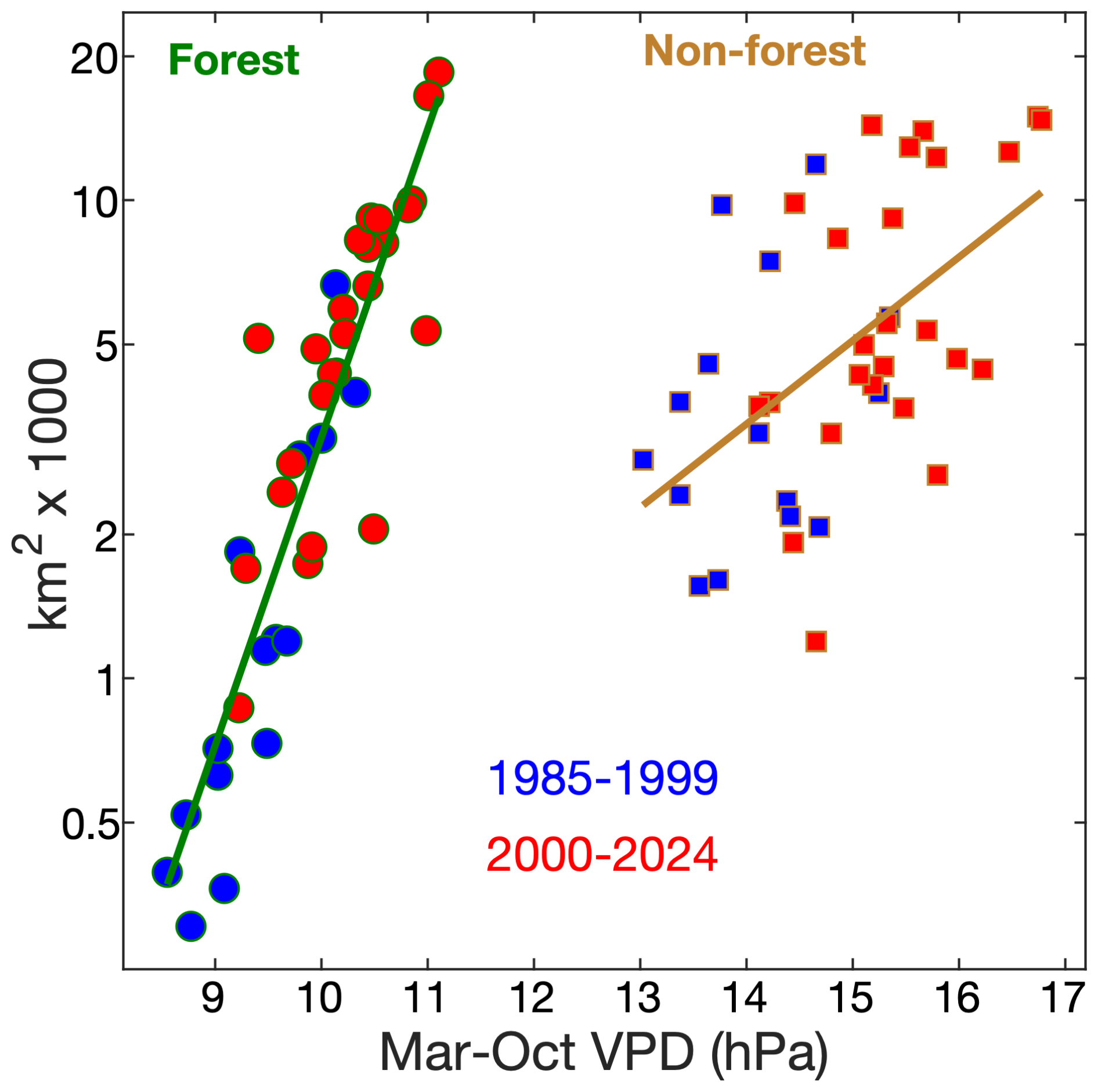
Figure 2 Annual wildfire area versus atmospheric aridity. Regressions are shown for forested (circles with green outlines) and non-forested (squares with brown outlines) areas of the western US. The vapor-pressure deficit (VPD) is a measure of the aridity of the atmosphere and March–October (Mar–Oct) is a time period when VPD is particularly strongly correlated with annual area burned. Fire and climate data are described in Sect. 3.1 and 3.3.

Fuel characteristics are also key determinants of wildfire activity, in part because they modulate the sensitivity of fire to climate (Bradstock, 2010; Littell et al., 2018). As long there are sufficient lightning or human ignitions, increased abundance and connectivity of flammable fuels will make fire activity more responsive to aridity. In non-forested areas of the western US, where fuels are generally more limiting due to less biomass and connectivity, the relationship between area burned and aridity is considerably weaker than in forested areas (Fig. 2, right side) despite non-forest areas on average being warmer, drier, and therefore more likely to burn based on fuel moisture alone.

Fuel characteristics also modulate how fire responds to climate within forests, and thus fire activity in a given region and time period may be strongly affected by that region's fire history. In a meta-analysis of >1000 western US forest fires, Parks et al. (2015) found a self-regulating effect of fire, where fuel reductions caused by past fires tended to limit subsequent fire spread for 5–20 years. In other meta-analyses, Parks et al. (2018a) and Hakkenberg et al. (2024) found that pre-fire fuel abundance, and ladder fuels in particular, strongly affect fire severity.

The US practice of fire exclusion has led to artificially high levels of vegetation biomass, spatial continuity, and understory vegetation in many western US forests (Hagmann et al., 2021). This has been especially detrimental for semi-arid forests where pre-European fire frequencies were on the order of 5–30 years (Swetnam, 1993; Swetnam and Baisan, 1996; Van de Water and Safford, 2011). In these forests, a century or more of little-to-no fire represents a dramatic departure from a historical fire regime typified by frequent, low-intensity surface fires. Resultant fuel accumulation has been conducive to vertical movement of fire into forest canopies (Steel et al., 2015; Hagmann et al., 2021). Accordingly, in many semi-arid western US forests, fire exclusion is partly responsible for the strength of the positive response of annual forest-fire area to warming and drying.

In the coming decades, continued changes to western US forest ecosystems due to changes in climate, fire regimes, and human activities will feed back to modify how fire sizes, frequencies, severities are affected by fluctuations and trends in climate (Williams and Abatzoglou, 2016; Littell et al., 2018; Buotte et al., 2019). For example, a continued rapid increase in forest-fire area may become increasingly self-regulating as fuel loads and connectivity decline (Parks et al., 2015, 2018b). Forecasting the timing, magnitude, and geography of this effect requires understanding of complex fire-induced mortality and succession (Harvey et al., 2016). In simulations with the LANDIS-II model, Hurteau et al. (2019) found that both coupled and uncoupled simulations resulted in large increases in area burned and fire emissions, but the coupled simulations had a small self-regulating effect that reduced projected trends by 10 %–15 %. However, LANDIS-II is computationally intensive, so this study was confined to three representative transects within the Sierra Nevada, rather than the whole Sierra Nevada. In addition, Hurteau et al. (2019) made simplifying assumptions that fire ignitions are randomly distributed across the landscape and fire effects on biomass only last for 10 years. Taking a much simpler approach, Abatzoglou et al. (2021) performed simulations treating the entire western US forest area as essentially a single model grid cell to assess how sensitive future western US trends in forest-fire area should be to the strength of fire's self-regulating effect. Even simulations that assumed a strong self-regulating effect projected continued rapid increases in forest fire area, though at only half the rate as simulations assuming no self-regulation. In addition to not considering spatial variability, Abatzoglou et al. (2021) focused solely on area burned and the simulations lacked ecological dynamics. As such, they modeled only until 2050 and did not assess the self-regulation effect on other variables such as fire intensity, severity, or biomass combusted.

Most wildfire impacts are caused by a relatively small number of fires (Moritz et al., 2005) and approximately 90 % of the total area burned in the western US is accounted for by fewer than 10 % of wildfires (Short, 2022). Given that larger fires tend to burn at higher severity (Cova et al., 2023), realistic simulation of future fire-vegetation coupling requires modeling extreme fire events. For realistic simulations of complex processes, a mechanistic modeling approach that explicitly simulates fine-scale processes such as combustion and energy transfer is ideal. However, the temporal and spatial scales at which fine-scale mechanistic fire models can be run are severely limited by computational constraints. For example, coupled atmosphere/fire models such as HIGRAD/FIRETEC (Linn, 1997; Linn et al., 2012), CAWFE (Coen, 2013) and WRF-Fire (Muñoz-Esparza et al., 2018) can only feasibly operate at a scale of tens of kilometers at most, insufficient to understand the drivers of historical and future wildfire activity across the large scale of the western US. One model designed for efficient simulation of fire dynamics across regions as large as the western US is SPITFIRE (Thonicke et al., 2010; Lasslop et al., 2014), which is described as process-based because it simulates fire intensity and wind-driven fire spread following Rothermel's equations (Rothermel, 1972; Andrews, 2018). However, the rules that govern ignitions and whether fuels are abundant and dry enough to burn are empirically parameterized. An advantage of mechanistic, or process-based, models is that they are deterministic; a given set of predictor conditions will always lead to the same fire outcome, making them diagnosable and replicable. Their disadvantage is that at the relatively low spatial and temporal resolutions necessary for decadal to centennial simulations across a large region like the western US, a model like SPITFIRE is likely to underrepresent variability and extremes.

Due to the limitations of all other forest-fire models, we developed a new stochastic forest-fire model for the western US, WULFFSS. We designed this model to operate in a coupled framework within a forest ecosystem model, the Dynamic Temperate and Boreal Fire and Forest-Ecosystem Simulator (DYNAFFOREST) (Hansen et al., 2022). The WULFFSS simulates the monthly occurrences and sizes of forest fires ≥1 km² in size on a 12 km resolution grid. Fire probabilities and sizes are determined as functions of fuel characteristics, topography, human population, and climate/weather. WULFFSS reproduces realistic spatiotemporal variations in fire frequency and area burned under historical conditions, and its use of conventional statistics promotes interpretability of model behavior and outputs. The model's computational efficiency and stochastic nature allow for many simulations of monthly forest-fire activity across the western US for decades or centuries at a time. Implementation of WULFFSS within a forest ecosystem-model such as DYAFFOREST will allow for simulation of the coupled interactions between fire and ecosystems that will ultimately shape how the western US forest-fire regime evolves under anthropogenic climate change. While WULFFSS is built to be coupled with DYNAFFOREST, it is designed in a modular fashion where coupling with other vegetation models should be relatively straight forward.

2 Geographic domain

Our study area is the forested domain of the eleven westernmost states of the coterminous US: Arizona, California, Colorado, Idaho, Montana, New Mexico, Nevada, Oregon, Utah, Washington, and Wyoming. Consistent with other work in the region (Buotte et al., 2019; Hansen et al., 2022), we determine the forested domain from the 250 m forest map from Ruefenacht et al. (2008), from which we calculate a 1 km resolution map of fractional forest coverage. We classify a given 1 km grid cell as forested if ≥50 % of the 250 m grid cells are forest. From this 1 km forest map, we determine our 12 km resolution model domain to include all 12 km grid cells containing at least one forested 1 km grid cell. We remove 12 km grid cells immediately south of the Canadian border because some of our landcover- and population-related predictor variables require information from surrounding grid cells. In total, there are 11 132 12 km grid cells within our forested western US study domain (Fig. 3). In assessments of regional model performance we consider the four quadrant regions mapped in Fig. 3: Pacific Northwest (PNW), Northern Rockies (N Rockies), California and Nevada (CA/NV), and the four-corner states (4 Corners).

Figure 3 The western US study domain. Grey contours outline the western US forested study region. Shades from white to green: fractional forest cover in each 12 km grid cell within the forested study region according to Ruefenacht et al. (2008). Orange dots: ignition locations of forest fires ≥100 ha in the study region from 1985–2024. Yellow: non-forested areas of the western US. Grey: outside the western US. Colored boundaries identify the four quadrant regions considered in regional analyses: Pacific Northwest (red, PNW), Northern Rockies (blue, N Rockies), California and Nevada (green, CA/NV), and the four-corner states (purple, 4 Corners).

3 Data

3.1 Forest fire

To parameterize the fire model we use the Western US MTBS-Interagency (WUMI2024a) database of observed wildfires from 1984–2024 (Williams et al., 2025). Like its predecessor described by Juang et al. (2022), the WUMI2024a was developed by harmonizing several public US government sources and it does not include fires <1 km² in size. The WUMI2024a contains a list of western US wildfire events, including ignition date, ignition location, and final fire size, as well as fire perimeters and 1 km resolution maps of the area burned for each fire. See Williams et al. (2025) for details about the data sources and the methods underlying the WUMI2024a. We constrain calibration of the WULFFSS to 1985–2024 due to a suspicious absence of fires from Wyoming and New Mexico in 1984.

We estimate forest area burned by each fire in the WUMI2024a and only retain fires that burned ≥1 km² of forest area. To estimate the forest area burned by each fire, we multiply each 1 km grid cell of fractional area burned by the fractional forest area and then sum. Of the 21 570 wildfires represented in the WUMI2024a in 1985–2024, 7639 have ≥1 km² forest area burned. However, a number of wildfires are identified in the WUMI2024a as “parent fires” composed of smaller sub-fires. This occurs because, although the most accurate dataset feeding into the WUMI2024a is the MTBS, that dataset sometimes attributes burned areas from multiple fires to a single event. The WUMI2024a notes these cases, and we replace parent fires with their associated sub-fires. To keep burned areas consistent with the high-quality calculations from MTBS, we re-scale the forest area burned by each set of sub-fires so that they sum to the parent fire's value. In cases where a sub-fire's ignition location is not within a 1 km forested grid cell that burned, we reassign the ignition location to the nearest grid cell with forest area that burned. We find 56 parent fires composed of at least two sub-fires with ≥1 km² forest area burned after rescaling. After replacing parent fires with their sub-fires, our dataset consists of 7799 wildfires with ≥1 km² forest area burned from 1985–2024. This number is reduced to 7635 after removing fires ignited in areas outside our western US study domain shown in Fig. 3 because they ignited near the Canadian or Mexican border or in a 12 km grid cell containing no 1 km grids with ≥50 % forest area.

3.2 Topography

We calculate topographic predictors from the 1 km digital elevation model produced by the NOAA GLOBE project (Hastings and Dunbar, 1998). From the 1 km grid of mean elevation we calculate 1 km grids of slope and aspect. We then calculate 12 km grids of mean slope to represent steepness as well as the standard deviation of 1 km elevation values to represent terrain ruggedness.

3.3 Climate

3.3.1 Daily $\mathrm{1}/\mathrm{24}$° gridded climate

We calculate climate predictors from daily gridded climate data with $\mathrm{1}/\mathrm{24}$° (∼4 km) geographic resolution for January 1951–December 2024. This period begins in 1951 rather than coincident with our 1985–2024 study period because the longer climate record is used to spin-up our forest simulations (Sect. 3.4). Daily variables are precipitation total (prec, mm), maximum temperature (tmax, °C), minimum temperature (tmin, °C), vapor pressure (ea, hPa), mean downwelling solar radiation at the surface (solar, W m⁻²), and mean 2 m wind speed (wind, m s⁻¹). For prec, tmax, and tmin, data come from the $\mathrm{1}/\mathrm{24}$°-resolution nClimGrid Daily dataset produced by the National Oceanic and Atmospheric Administration (Durre et al., 2022), which covers 1951–present. For ea we apply the Clausius Clapeyron formulation to the daily $\mathrm{1}/\mathrm{24}$°-resolution dew point (tdew, °C) dataset from the PRISM group at Oregon State University (Daly et al., 2021). This dataset is better than reanalysis products because it is based on station observations. However, the daily PRISM dataset starts in 1981. For 1951–1980, we use a dynamically-downscaled version of the ERA5 reanalysis for the western US (Rahimi et al., 2022). This reanalysis has 9 km spatial resolution and covers September 1950–April 2025. We use daily outputs of mean specific humidity (q, m³ m⁻³) and surface pressure (p, hPa) to estimate ea: $pq/(\mathrm{0.622}+\mathrm{0.378}q)$. We then bilinearly interpolate to $\mathrm{1}/\mathrm{24}$° resolution and use quantile mapping to bias correct the Rahimi et al. (2022) data such that, for each grid cell and each of the 12 months, the distributions of daily ea estimated from Rahimi et al. (2022) match those estimated from PRISM during their period of overlap. For solar and wind, we prioritize the daily outputs from Rahimi et al. (2022) because there are no long-term spatially continuous records of direct observations of these variables and the Rahimi et al. (2022) data have uniquely high spatial resolution and long temporal coverage. We downscale the Rahimi et al. (2022) solar and wind data to $\mathrm{1}/\mathrm{24}$° resolution using bilinear interpolation.

For solar, we account for the effect of slope and aspect on incident solar angle (e.g., solar intensity is higher on south-facing slopes). The Rahimi et al. (2022) reanalysis accounts for the effect of elevation on solar intensity, but not the effect of slope and aspect. To do this, we used the 1 km maps of slope and aspect described in Sect. 3.2. Our method is to, for each day in a generic 365 d year and assuming a top-of-atmosphere solar constant of 1367 W m⁻², use the method developed by Kumar er al. (1997) to estimate the mean downwelling solar intensity at the surface at 1 km resolution for two scenarios: one with observed elevation, slope, and aspect (solar_topo) and another with observed elevation but assuming a flat topography within each 1 km grid cell (solar_flat). For each day we then calculate an adjustment factor representing the fractional effect of slope and aspect on incident solar radiation at the surface as solar_adj = solar_topo$/$solar_flat. We then upscale the daily grids of solar_adj to $\mathrm{1}/\mathrm{24}$° resolution and calculate a topography-adjusted version of solar (solar_topo) by multiplying each daily map of solar by its corresponding map of solar_adj.

We use the $\mathrm{1}/\mathrm{24}$° daily climate maps described above to calculate a number of fire-relevant derived variables. We calculate daily mean VPD as the average of the daily maximum and minimum VPD (VPDmax and VPDmin, respectively), where VPDmax is calculated as the saturation vapor pressure (es) at tmax minus ea and VPDmin is calculated using es at tmin. As a metric representing daily atmospheric fire weather, we use a modified version of the hot-dry-windy index (HDWI, hPa m s⁻¹) representing surface conditions. The standard formulation of the HDWI (Srock et al., 2018) multiplies wind by VPD at multiple vertical levels within the bottom 500 m of the atmosphere on a sub-daily time scale (e.g., 6-hourly), and then defines each day's HDWI value as the maximum among all values from at any vertical level or time step. Our simplified approach is to estimate daily HDWI as VPDmax multiplied by wind.

To represent the effect of snowpack we use the 4 km daily gridded climate data to simulate daily mean snow-water equivalent (SWE, mm) using the SnowClim model (Lute et al., 2022), which is designed for efficient simulation of western US snow dynamics in response to gridded forcing data at a daily or sub-daily time step.

To represent fuel moisture we calculate the daily 100 and 1000 h dead fuel moisture content (FM100 and FM1000, respectively, %) following the method of the National Fire Danger Rating System (NFDRS) (Cohen and Deeming, 1985). The 100 and 1000 h fuel classes represent woody fuels 25–76 mm and 76–203 mm in diameter, respectively, and the names of the fuel classes represent the approximate e-folding time required for moisture content to equilibrate with the atmosphere. We include the effect of simulated snow in our calculations by setting relative humidity to 100 % when the snow depth is ≥5 mm and by withholding precipitation that increases the water content of the snowpack until it melts out of the snowpack.

3.3.2 Monthly 12 km climate predictors

We calculate nearly all monthly climate predictors from the daily $\mathrm{1}/\mathrm{24}$° grids described above. In addition to monthly means we also consider variables representing fire-relevant sub-monthly quantities (e.g., maximum 1 or 3 d mean HDWI or VPD, maximum single-day SWE of the past 12 months) as well as variables representing the integration of climate conditions over multiple months (e.g., 3, 6, 9, or 12 month mean VPD).

In addition to 12 km climate predictors derived from our daily $\mathrm{1}/\mathrm{24}$° dataset, we also consider lightning frequency using the 0.1°-resolution daily maps of lightning-strike density from the National Lightning Detection Network (NLDN, https://www.ncei.noaa.gov/pub/data/swdi/, last access: 26 March 2025). This dataset begins in 1987 and we aggregate to monthly maps of 12 km lightning frequency for 1987–2024. However, NLDN methodology changed over time so we only use maps of long-term and monthly climatological mean lightning frequencies as predictors. To account for temporal variability in lightning potential on interannual timescales, we consider monthly mean convective available potential energy (CAPE) as well as maximum 1 and 3 d mean CAPE from Rahimi et al. (2022), which we upscale to 12 km resolution using bilinear interpolation.

3.4 Landcover

Due to a lack of spatially continuous and temporally evolving observational maps of fire-relevant forest biomass variables throughout our study period, we simulate forest biomass during our study period using the Dynamic Temperate and Boreal Fire and Forest-Ecosystem Simulator (DYNAFFOREST) (Hansen et al., 2022). DYNAFFOREST is a process-based forest ecosystem model designed to efficiently simulate forest dynamics across the western US at a medium spatial resolution (grid cell size of 1 km²). The model represents 11 forest types and one grass/shrub type, runs at an annual time step, and simulates a suite of variables representing various stand structure characteristics and ecosystem functions. DYNAFFOREST is a cohort based model. In each forested 1 km grid cell, a single tree representing one forest type is simulated. Simulated metrics from the single tree are then used to estimate stand structural characteristics for each grid-year, such as stand age, density, basal area, mean canopy height, and diameter at 1.35 m above the ground. DYNAFFOREST tracks 3 live and 3 dead above-ground biomass pools: stem, branch, and foliage, and standing snags, downed coarse wood, and forest floor litter. Cohort mortality occurs probabilistically as a function of background causes, drought, and fire.

When a fire occurs, DYNAFFOREST estimates percent crown kill of the cohort as a function of fuel aridity, tree size, and forest-type specific crown dimensions. Probability of mortality is estimated as a function of crown kill and bark thickness. Following a fire, forest establishment and recovery is simulated in DYNAFFOREST probabilistically based on the fecundity of the surrounding forest types, dispersal distance in the target grid cell and surrounding grid cells, and the effects of climate on seed germination and establishment. Key functional traits related to postfire recovery, like cone serotiny and asexual resprouting, are included. If stand-replacing fire occurs and postfire establishment does not occur the next year, then the landcover is assumed to convert to grass/shrub, though forest can return when seed supplies and climate conditions allow.

Because DYNAFFOREST outputs are not observational, our empirically parameterized fire model will not perfectly represent how observed forest characteristics affect the probabilities and sizes of forest fires. However, DYNAFFOREST has been well benchmarked across large diverse forest types of the western US (Hansen et al., 2022) and used to simulate coupled fire-forest relations in the context of fuels management (Daum et al., 2024). Additionally, we find reasonable representation of ecoregional differences in most above-ground biomass pools when we compare DYNAFFOREST outputs with the US Forest Service's Forest Inventory and Analysis survey data (USDA Forest Service, 2019). Further, in the DYNAFFOREST simulation used to produce the 1985–2024 forest maps that we use to parameterize the fire model, we apply the observed 1 km maps of forest area burned from WUMI2024a. By allowing DYNAFFOREST to simulate forest responses to known fires, our parameterization reflects not just the effects of naturally occurring, long lasting gradients in forest condition on fire, but also more transient, sharper gradients caused by prior fires.

To assure realistic and stable forest dynamics leading into the 1985–2024 parameterization period, we conduct a >334 year spin-up using WULFFSS coupled with DYNAFFOREST. For the first 300 years (1651–1950), we force DYNAFFOREST with detrended climate data from 1901–1950 and climate years are randomly selected with replacement. For 1951–1984, we use observed climate so that forest condition in the WULFFSS parameterization can reflect the legacies of recent climate variations. With the exception of the variables used to force WULFFSS, the climate variables used by DYNAFFOREST are mean June–August 0–100 cm soil moisture and annual forest-type specific temperature metrics such as growing-degree days and freezing-degree days. Monthly 0–100 cm moisture is modeled from monthly 12 km climate data from 1901–2024 following Williams et al. (2017, 2020) and bilinearly interpolated to 1 km resolution. The temperature metrics are calculated from monthly $\mathrm{1}/\mathrm{24}$° grids of mean tmax and tmin. We downscale the $\mathrm{1}/\mathrm{24}$° grids to 1 km resolution guided by the TopoWx dataset (Oyler et al., 2015). Specifically, TopoWx provides monthly grids of tmax and tmin from 1948–2016 with resolutions of $\mathrm{1}/\mathrm{24}$ and $\mathrm{1}/\mathrm{120}$° (∼800 m). For each month and variable, we use the $\mathrm{1}/\mathrm{120}$° version to calculate a mean 1980–2016 climatology with 1 km resolution (estimating 1 km values from the $\mathrm{1}/\mathrm{120}$° grid using nearest-neighbor interpolation) and then produce a 1 km map of offsets that relate each 1 km climatological mean value to its overlying $\mathrm{1}/\mathrm{24}$°-resolution value from the same years. We apply the offsets to the monthly mean tmax and tmin from NOAA nClimGrid (Vose et al., 2014) to produce 1 km maps of monthly mean tmax and tmin from 1901–2024. Thus, we force the non-fire portion of the DYNAFFOREST simulations with observed climate data for the 1901–2024 period.

Due to lack of fine-scale data on forest ecosystems from the pre-spin-up period, we initialize the spin-up using a 1 km resolution map of observed modern forest types that we derived from the Ruefenacht et al. (2008) map of forest types. Initial fuel loads are representative of the 11 forest types and the biomass pools stabilize after approximately 250 years of spin-up.

For landcover variables not simulated by DYNAFFOREST, we use the maps of land-cover type from the US Geological Survey's National Land Cover Database (NLCD; https://www.usgs.gov/centers/eros/science/annual-national-land-cover-database, last access: 8 January 2025). The NLCD provides annual maps of landcover classifications at 30 m resolution across the US for 1985–2024. Because the NLCD map for a given year often reflects the effects of fires during that year, and we do not wish to mistake the effects of fires for their causes, we consider each year's landcover to be represented by the prior year's NLCD map (for 1951–1985 we assign the 1985 landcover). From these 30 m maps of landcover we calculate 1 km maps of fractional coverage for four non-forest categories: unburnable (water, ice, wetland, barren), developed (low, medium, high intensity), agriculture (cultivated, pasture, developed open space), and grass/shrub (grass/herb, shrub/scrub). For each year from 1951–2024 we rescale these fractional coverages so that, for grid-years where the DYNAFFOREST simulation does not indicate forest coverage, these non-forest classes sum to full coverage. Likewise, for grid-years where DYNAFFOREST simulates forest coverage, we set the non-forest types to zero.

In addition to 1 km maps of aboveground forest biomass density (in distinct pools and in total), mean canopy height, mean diameter at breast height, and fractional coverage by landcover type, we also calculate 1 km maps of forest connectivity. We define this as, for each 1 km grid cell, the fraction of adjoining grid cells with ≥10 000 kg ha⁻¹ live biomass density, which corresponds to approximately the 5th percentile of all simulated 1 km² live biomass density values for 1985–2024. Specifically, for each 1 km grid cell with ≥10 000 kg ha⁻¹ live biomass we calculate the number of consecutive adjoining grid cells in each of the 8 directions radiating away from the central grid cell that also have ≥10 000 kg ha⁻¹ live biomass. In each of the four directions radiating north, south, east, and west, we consider the 6 nearest grid cells. In each of the four diagonal directions we consider the nearest 4 grid cells. We then calculate connectivity as 1 (for the central grid cell) plus the sum of the total number of adjoined grid cells with ≥10 000 kg ha⁻¹ grid cells the 8 directions divided by the number of grid cells considered (41). This approach allows for efficient recalculations of connectivity when simulations are run in coupled mode with DYNAFFOREST and the size of the area represented is roughly aligned with that of a large wildfire 10 000 ha in size.

From the 1 km grids of annual forest properties and fractional coverage by landcover type described above we calculate 12 km maps of averages within each 12 km grid cell. Given that fire sizes can also be influenced by landcover beyond the ignition location, we also consider variables that represent spatial averages within the area of a very large 500 km² (50 000 ha) fire, which we approximate as a 23 km×23 km square. Likewise, our use of sub-12 km landcover data to produce landcover predictors allows our modelling to include the effects of within-grid heterogeneity of fuel conditions, which is important given that most fires are smaller than 144 km².

3.5 Human population and roads

Humans cause approximately half of all ignitions (Balch et al., 2017) and attempt to suppress almost all wildfires in the western US. We therefore include predictor variables related to population density and distance to populated areas. Because the US Census changed how it provides population information in 2020, so that reported numbers are sometimes swapped among Census units (“blocks”) to maintain confidentiality, we work with census-based housing-unit density instead. Specifically, we use the shapefiles of census-based, block-level housing density in 2000, 2010, and 2020 developed by the SILVIS Lab (https://silvis.forest.wisc.edu/data/wui-change/, last access: 20 May 2024) (Radeloff et al., 2018, 2023). For 1950–1990 we use decadal hindcast maps of housing density produced by the SILVIS Lab using partial block-group level census data. For 2030, which is used with 2020 to interpolate housing density for 2021–2024, we use a projection based on county-level forecasts of housing density from Woods & Poole Economics (https://www.woodsandpoole.com/our-databases/united-states/, last access: 20 May 2024), which is downscaled to the block level by the SILVIS Lab based on 2020 housing density patterns. For each decade we rasterize the polygon data to a 1 km grid of housing density. We then produce annual maps of 1 km housing density for 1951–2024 by linearly interpolating between the decadal maps.

From the annual 1 km maps of housing density we produce two sets of 1 km maps to represent distance from populated areas. In the first, we map the distance to the nearest grid cell with ≥5 housing units per km² to represent distance to a relatively sparsely populated community. In the second we map the distance to the nearest grid cell with ≥50 housing units per km² to represent distance from a more heavily urbanized area.

Related to population, we also consider spatiotemporal variations in total and per-capita gross domestic product (GDP) as proxies for variations in fire-suppression capacity. We use the annual 0.5°-resolution maps of GPD and GDP per capita from 1990–2022 from Kummu et al. (2025) and bilinearly downscale to 12 km resolution.

The geographic distribution of ignitions and fire-suppression activities also depend on roads. We use the 2013 Global Roads Open Access Data Set, Version 1 (gROADSv1; https://search.earthdata.nasa.gov/search/granules?p=C1000000202-SEDAC, last access: 17 September 2024). This dataset specifies for each road segment a Functional Class: Highway, Primary, Secondary, Tertiary, Local/Urban, Trail, Private, or Unspecified. We aggregate these into two classes: major (Highway and Primary) and minor roads (all others). We then produce 1 km maps of the distance to the nearest major road, distance to nearest minor road, and distance to nearest road of any class. We treat the road network as static in time due to unavailability of construction or closure dates.

Finally, we calculate 12 km maps of mean 1 km housing density, distance to nearest location with ≥5 or ≥50 housing units per km², and distance to nearest major road, minor road, or any road as predictor variables in the forest-fire model.

4 Model description

The WULFFSS model has a spatial resolution of 12 km across the forested domain of the western US (Fig. 3) and operates monthly. The model is parameterized on the dataset of 7635 forest-fire locations and sizes described in Sect. 3.1. A schematic visualizing the general framework of WULFFSS is provided in Fig. 4.

Figure 4 Flowchart outlining the general framework of the WULFFSS.

WULFFSS consists of three statistical models, loosely following Westerling et al. (2011). The general framework is that first model estimates, for each grid-month, the probability of ≥1 wildfire (P) from a multi-variate logistic regression with predictor variables representing landcover, topography, humans, and climate. To account for the possibility of >1 wildfire in a given grid-month, the second model uses P as a single predictor in a logistic regression to estimate the probability that any given number of wildfires occurs in each grid-month (N). The third model is a fire-size model that uses multi-variate regression to estimate the forest area burned (A) by each wildfire as a function of landcover, topography, humans, and climate, similar to the P model.

The P and A models each consist of three components representing spatial variability (S), the mean annual cycle (C), and temporal anomalies (T), as well as interactions between these components (SC, ST, and CT). The S component is constructed first to capture how variations in fire activity are driven by factors that are far more variable in space than in time, as these factors (e.g., forest biomass, lightning frequency, variables related to human population and fire suppression) are likely to modulate the sensitivity of fire activity to temporal variables. The C component is then constructed to account for variations in fire activity that are due to the mean annual climate cycle. Finally, the T component is constructed to account for effects of climate variations on timescales of interannual and longer, which are likely to be strongly modulated by the effects of the S and C variables already accounted for.

The S component represents drivers of forest-fire occurrence or size that are most variable in the spatial domain, such as topographic slope, fuel availability, human population, mean annual lightning frequency, and long-term mean aridity, all of which may directly influence fire occurrence and also modulate the effects of C and T. Each potential S predictor is standardized such that all grid-month values in the study domain have a mean of 0 and standard deviation of 1 for the calibration period (1985–2024). Many S predictors represent alternate expressions of a single predictor, for example house density, log₁₀(house density), mean house density within 50 kha, and log₁₀(mean house density within 50 kha). Logarithmic transformations are made on many of the S variables to give these variables more Gaussian distributions.

The C component represents climatological drivers of forest-fire occurrence or size that are most variable in the domain of the mean annual cycle, such as long-term means of each month's lightning frequency as well as variables that influence the seasonality of fuel moisture such as prec, solar, and VPD. For all potential C predictors, mean annual cycles are calculated based on the calibration period. As for S, most potential C variables are permutations of common variables. For example, the effects of climate variables related to fuel moisture may accumulate over several months, so the annual cycle of each climate variable is considered as 1, 2, 3, 4, and 5 month running means. Further, two versions of most C variables are considered. In the first, each grid cell's mean annual cycle is scaled from 0–1, where 0 and 1 represent the mean annual minimum and maximum, respectively, so all spatial variability is due to variability in the timing of the annual cycle. In the second, mean annual cycles are not scaled and these variables retain spatial differences in each month's mean conditions. For each of these unscaled C variables, values are standardized relative to all calibration-period grid-months.

The T component represents climatological drivers of forest-fire occurrence or size that are most variable in the temporal domain of interannual and longer. Potential T predictors include the standardized precipitation index (SPI) (McKee et al., 1993), frequency of wet days with ≥2.54 mm prec (Holden et al., 2018), FM1000, FM100, VPD, solar, HDWI, CAPE, and SWE. As for C, many potential T variables are permutations to represent cumulative effects over various ranges of months. In addition, monthly measures of some sub-monthly meteorological conditions are considered such as the highest 1 or 3 d mean VPD within a month. Because T is meant to represent climate variability beyond the annual cycle, T variables are standardized so that for a given variable in a given grid cell, values have a mean of 0 and standard deviation of 1 for each of the 12 months during the calibration period.

In both the P and A models, each of the three components is represented by a single composite index that expresses the combined effect of multiple predictor variables. The variables that contribute to each of the three components (S, C, and T) are selected stepwise and only retained if they contribute significantly to model skill (see Sect. 4.1). Thus, each model ultimately uses only a subset of the potential predictors. Lists of all potential predictors are listed in Tables A1–A3 (see Tables S1–S3 in the Supplement for variable descriptions). For some variables, it is logical that the effect on P or A should be only positive or negative. For example, the direct effect of fuel availability on fire occurrence and size is far more likely to be positive than negative, but a statistical model may detect a hump-shaped or even negative relationship due to the co-occurring influences of moisture on fuel availability (positive) and flammability (negative) (Bradstock, 2010; Krawchuk and Moritz, 2011). To avoid including unrealistic effects due to co-linearities or model overfitting, we do not allow some predictors to be included if the sign of their effects are inconsistent with our understanding of western US forest fire (see Tables A1–A3).

4.1 Model framework

We use stepwise multiple regression to build the P and A models. We use multiple logistic regression to calculate our estimates of P (P_est):

$$\begin{array}{}\text{(1)}& P_{\text{est}}=\mathrm{1}/(\mathrm{1}+{\mathrm{e}}^{-{\mathbf{X}}_P{\mathit{\beta }}_P})\end{array}$$

where β_P is a vector of logistic regression coefficients and X_P is a matrix of the three S, C, and T composite predictors (S_P, C_P, and T_P, respectively), as well and their interaction terms (S_PC_P, S_P,T_P, and C_P,T_P), such that

$$\begin{array}{}\text{(2)}& \begin{array}{rl}{\mathbf{X}}_P{\mathit{\beta }}_P=& {\mathit{\beta }}_{P\mathrm{0}}+{\mathit{\beta }}_{P\mathrm{1}}{S}_P+{\mathit{\beta }}_{P\mathrm{2}}{C}_P+{\mathit{\beta }}_{P\mathrm{3}}{T}_P+{\mathit{\beta }}_{P\mathrm{4}}{S}_P{C}_P\\ & +{\mathit{\beta }}_{P\mathrm{5}}{S}_P{T}_P+{\mathit{\beta }}_{P\mathrm{6}}{C}_P{T}_P.\end{array}\end{array}$$

Each of the three composite predictors, S_P, C_P, and T_P, represents contributions from a number of S, C, and T variables, where each S, C, and T variable included has been selected in a stepwise process and transformed to linearize its relationship with P following methods described below.

To model A, we follow a similar approach as for P except that we use multiple linear, rather than logistic, regression to estimate size-weighted and normalized anomalies of A (Az_w; details in Sect. 4.4):

$$\begin{array}{}\text{(3)}& A{z}_{\mathrm{w}}={\mathbf{X}}_A{\mathit{\beta }}_A,\end{array}$$

where β_A is a vector of linear regression coefficients and X_A is a matrix of S, C, and T composite variables (S_A, C_A, and T_A, respectively) and their interactions (S_AC_A, S_A,T_A, and C_A,T_A) such that

$$\begin{array}{}\text{(4)}& \begin{array}{rl}{\mathbf{X}}_A{\mathit{\beta }}_A=& {\mathit{\beta }}_{A\mathrm{0}}+{\mathit{\beta }}_{A\mathrm{1}}{S}_A+{\mathit{\beta }}_{A\mathrm{2}}{C}_A+{\mathit{\beta }}_{A\mathrm{3}}{T}_A+{\mathit{\beta }}_{A\mathrm{4}}{S}_A{C}_A\\ & +{\mathit{\beta }}_{A\mathrm{5}}{S}_A{T}_A+{\mathit{\beta }}_{A\mathrm{6}}{C}_A{T}_A.\end{array}\end{array}$$

We considered including three-way interactions between the S, C, and T predictors in the P and A models but doing so did not improve model skill. In the rest of this subsection we describe the parts of the model-building framework that are common to the P and A models. Details specific to just the P or A model will be described in Sect. 4.2 and 4.4, respectively.

Both models are built sequentially, first constructing the spatial composite predictor (S_x, where subscript x is P for the P model or A for the A model). Next the annual cycle composite predictor (C_x) and its interaction with S_x (S_xC_x) are built. Finally the temporal anomaly predictor (T_x) and its interactions with S_x and C_x (S_xT_x and C_xT_x, respectively) are built.

To construct S_x, we first assess the general shape and strength of the relationship between each potential S predictor and the variable we are modeling, x, using a binned regression. We sort each potential S_x predictor into equally sized bins (45 for the P_x model and 25 for the A_x model), and calculate the mean of x for each bin. For each potential predictor we then regress the binned mean x values against the means of the binned predictor values and quantify the relationship using linear, quadratic, and cubic fits. The accuracy of each fit is assessed with the Akaike Information Criterion with a correction for low sample size (AICc) (Akaike, 1974; Hurvich and Tsai, 1989) and penalty for higher-order fits. Curve fits resulting in AICc>0 are immediately dismissed. Among the remaining curve fits, a Monte Carlo significance test is conducted in which x is randomized and re-binned 100 times for the P model and 200 times for the A model. Curve fits are only considered if the actual AICc is more negative than at least 95 % of the AICc values from the Monte Carlo test. Finally, the variable and curve fit combination with the most negative AICc is tentatively accepted as the initial predictor (V_S1) to represent S_x. Specifically, V_S1 is calculated by applying the selected curve fit to all the values of the selected variable and then S_x is calculated by standardizing V_S1 relative to a mean of 0 and standard deviation of 1. An initial version of the model is then developed by applying S_x as the single variable to estimate x. Model accuracy is assessed as correlation between modeled and observed values of x (see Sect. 4.2 and 4.4 for details about the correlation tests specific to the P and A estimates). At this point in the model-building process, the model coefficients and correlation values are recalculated 100 times when V_S1 values are randomly reordered (200 times for the A model). If the model's correlation value is not >95 % of the alternative correlation values, then the variable under consideration is dismissed and we consider the potential predictor that led to the next lowest AICc value in the binned regression analysis.

After S_x is initially created from a single variable, we calculate residuals in x and explore whether additional S variables should be included within S_x. We do this by regressing binned means of the residuals, representing variance in x not yet accounted for by the model, against the binned values for all potential S_x predictors still under consideration. Notably, if the predictor variable selected in the previous step has a log₁₀ counterpart, or vice versa, the counterpart is not considered in subsequent model-building steps. As before, only curve fits resulting in a negative AICc and satisfying the Monte Carlo significance test are considered. If ≥1 curve fit satisfies these criteria, the variable and curve fit with the most negative AICc is passed on for further consideration as V_S2 by updating the calculation of S by adding V_S2 to V_S1 and re-standardizing. We then re-fit the regression equation using S_x to estimate the predictand and calculate an updated correlation between model estimates and observations. If the updated correlation is more positive than the previous correlation and is also more positive than 95 % of the Monte-Carlo generated correlations calculated with randomized V_S2 values, then the model is updated using V_S1 and V_S2. If these correlation criteria are not satisfied, the variable and curve fit that resulted in the next most negative AICc value is considered as a potential V_S2. This process is repeated until no additional variable and curve fit satisfies the above criteria for inclusion in S_x.

Next, the C_x component is added, constructed in the same stepwise manner as S_x, where a C variable is only included in C_x if (1) the binned regression with residuals leads to a negative AICc that is lower than 95 % of values produced when residuals are randomized in the Monte Carlo repetitions and (2) model estimates of x correlate more positively with observations than did the previous model's estimates and also more positively than 95 % of Monte Carlo correlations calculated when the C variable under consideration is scrambled randomly. A difference from construction of S_x is that now the model is a multivariate regression with three predictors: S_x, C_x, and their interaction, S_xC_x. To avoid nonsensical interactions in S_xC_x where two negative predictor anomalies would have the same effect as two positive anomalies, we positive-shift all S_x and C_x values by subtracting each predictor variable's minimum value before multiplying them. For the P model, we subtract the lowest S_P and C_P values to occur among all grid-months in the calibration period. For the A model, we subtract the lowest S_A and C_A values among grid-months that cooccurred with calibration-period fire. We then calculate S_xC_x as the standardized product of the positive-shifted S_x and C_x predictors such that the values of S_xC_x have a mean of 0 and standard deviation of 1.

Finally, the same methods are used to construct T_x to capture temporal variability not accounted for by S_x and C_x. With T_x included, the matrix of normalized predictors (X) includes all 6 predictor variables shown in Eqs. (2) and (4) (S_x, C_x, T_x, and 3 interactions).

Following parameterization of the initial models, we found that some potential predictor variables not selected initially could contribute significantly if considered in a second pass. This was unsurprising because each stepwise improvement to one component of the model affects the influence of the other components through interactions. We thus perform a second pass in the model-building process in which S, C, and T variables that were not selected in the original construction of S_x, C_x, and T_x are given another opportunity for inclusion. In addition, we consider a small number of variables that were not considered in the first pass. For example, some variables such as temporally varying SWE and fractional snow coverage do not fall cleanly into one of the three categories. Snow may be viewed as a landcover feature that inhibits fire spread or modulates the ability of climate anomalies to affect fuel moisture, in which case S is appropriate, but snow presence and amount are highly variable in time. Breaking snow qualities into monthly climatologies and standardized anomalies about those climatologies is not ideal, however, as SWE and fractional coverage are highly non-normal and dominated by zeros. We therefore allow, in the second round of stepwise model fitting, for monthly SWE and fractional snow coverage to be considered as both S and T variables. We also consider some additional S variables representing distance from road as well as landcover characteristics that are not outputs from the DYNAFFOREST model. These variables are only considered in the second round because (1) we do not have a temporally varying dataset of road networks and (2) we prefer that the effect of landcover on modeled fire is dominated by variables that we can simulate with DYNAFFOREST as coupled interactors with fire. Tables A1–A3 specify the variables we only consider in the second rounds model fitting.

4.2 The forest-fire probability model

To model P, we use all available grid-months in the observed 1985–2024 forest-fire dataset to fit a logistic regression (Eqs. 1 and 2). During this period, forest fires occurred in 7394 unique grid-months. For more efficient model parameterization and to avoid biasing the model with conditions under which large forest fires are exceedingly improbable, we exclude grid-months from our logistic regression where mean daily SWE exceeds the 99th percentile (0.76 mm) of values, leaving 7318 forest fires. Mean SWE exceeds this value in 20 % of calibration-period grid-months, leaving a sample size of 4 286 622 grid-months with which to parameterize the P model. Among these grid-months, the observed frequency of ≥1 forest fire is 0.0017.

We assess the accuracy of the logistic P model using the Matthew's correlation coefficient (MCC) (Matthews, 1975), which rewards correct classifications and penalizes against incorrect classifications. Because P_est is scalar (0–1), we convert P_est to 500 potential predictions of binary fire occurrence by, for each grid-month, drawing 500 random, uniformly distributed numbers from 0–1, predicting fire occurrence (1) in all cases where the random number is less than P_est, and predicting no fire (0) when the random number is greater than P_est. This allows for calculation of 500 MCC values and we consider the mean value to represent the MCC of the model.

To construct the S_p component we consider 54 potential predictors initially and 14 additional predictors in the second pass (Table A1). Variables and curve fits selected by the stepwise process to build the composite S_p predictor are shown in Fig. 5a. Variables not included in the original round of model fitting but added in the subsequent round are indicated by “2nd round” in Fig. 5.

Figure 5 Predictor variables and associated curve fits in the fire-probability (P) model. Variables are in three categories: spatial (S_p), mean annual climate cycle (C_p), and temporal climate anomalies (T_p). Y axis values in each panel indicate observed fire probabilities (P_obs; $\times {\mathrm{10}}^{-\mathrm{3}}$) not already accounted for prior to inclusion of that panel's predictor variable. Bars indicate the mean residual P_obs values among grid-months for which the predictor variable falls within each of 45 evenly spaced bins. Red lines/curves indicate the linear, quadratic, or cubic fit used to approximate the response of P_obs residuals to each predictor variable. With the exception of some C_p predictor variables, which are scaled from 0–1, predictors are expressed as standard-deviations from the mean. Statistics indicate each curve fit's low-sample-size Akaike Information Criterion (AICc) and the fraction of fits that produced a more negative AICc when the values being predicted are randomly scrambled prior to binning (p-value). Variable names are provided above each panel and are defined in Tables A1–A3. Panels representing variables selected in the second round of model fitting have grey text: “2nd round.”

The construction of S_p indicates that P_est is promoted by topographic slope, lightning frequency, high fractional forest coverage and forest connectivity, and high prior-year precipitation total where grass and shrub cover is abundant. P_est is reduced in areas of high housing density, near roads, in areas with high unburnable cover (barren land and water), and where the mean climatology is very wet (mean annual aridity index >2 standard deviations above the mean).

To construct C_p, we consider 48 potential predictors initially and 16 additional predictors in the second pass (Table A2, Fig. 5b). The annual cycle of P_est is dominated by annual cycles in fire weather (high HDWI), fuel moisture (as represented by wet-day frequency, VPD, and solar radiation), and lightning frequency.

To construct T_p, we consider 25 potential T predictors initially and 12 additional predictors in the second pass (Table A3, Fig. 5c). High P_est is promoted when FM100 is low, VPD has been anomalously high over the past 8–9 months, and in months with high HDWI and infrequent precipitation, but P_est can be suppressed if precipitation totals were anomalously low between 1.5 and 0.5 years ago.

The spatiotemporal distribution of P_est generally agrees well with observations (Fig. 6). However, there is a positive bias of P_est among very low values. In particular, among the grid-months that we excluded from model calibration due to mean daily SWE exceeding the 99th percentile, P_obs was 28.20 % of P_est. We therefore apply a bias adjustment to all grid-months with SWE exceeding the above threshold by multiplying P_est in these grid-months by 0.2820. Despite the bias correction for snowy grid-months, our model still systematically overestimates P_est among grid-months with low values of P_obs (Fig. 6a). Among the 50 % of 1985–2024 grid-months where P_est is below the median ($\mathrm{1.19}\times {\mathrm{10}}^{-\mathrm{4}}$), the mean P_obs is 52 % of modeled. This positive bias among very low values of P_est is strongest in PNW (Fig. 6a). We do not apply a further correction to account for this because the positive bias among low P_est values is of little consequence to the accuracy of the P model. The vast majority of fires are simulated to occur under higher P_est conditions; 96 % of simulated fires occur where P_est is above the median. Among these grid-months, P_est scales well with P_obs (Fig. 6a). This finding of consistently strong model skill where P_est is above-median holds at the regional scale as well (colored dots in Fig. 6a represent the 4 regions mapped onto Fig. 6b). Figure 6b further shows a realistic geographic distribution of mean P_est. Our model captures known areas of particularly high fire densities such as in California's Sierra Nevada and North Coast ranges, the mountainous areas of southern Arizona and New Mexico, and a relatively remote portion of the northern Rocky Mountains in central Idaho.

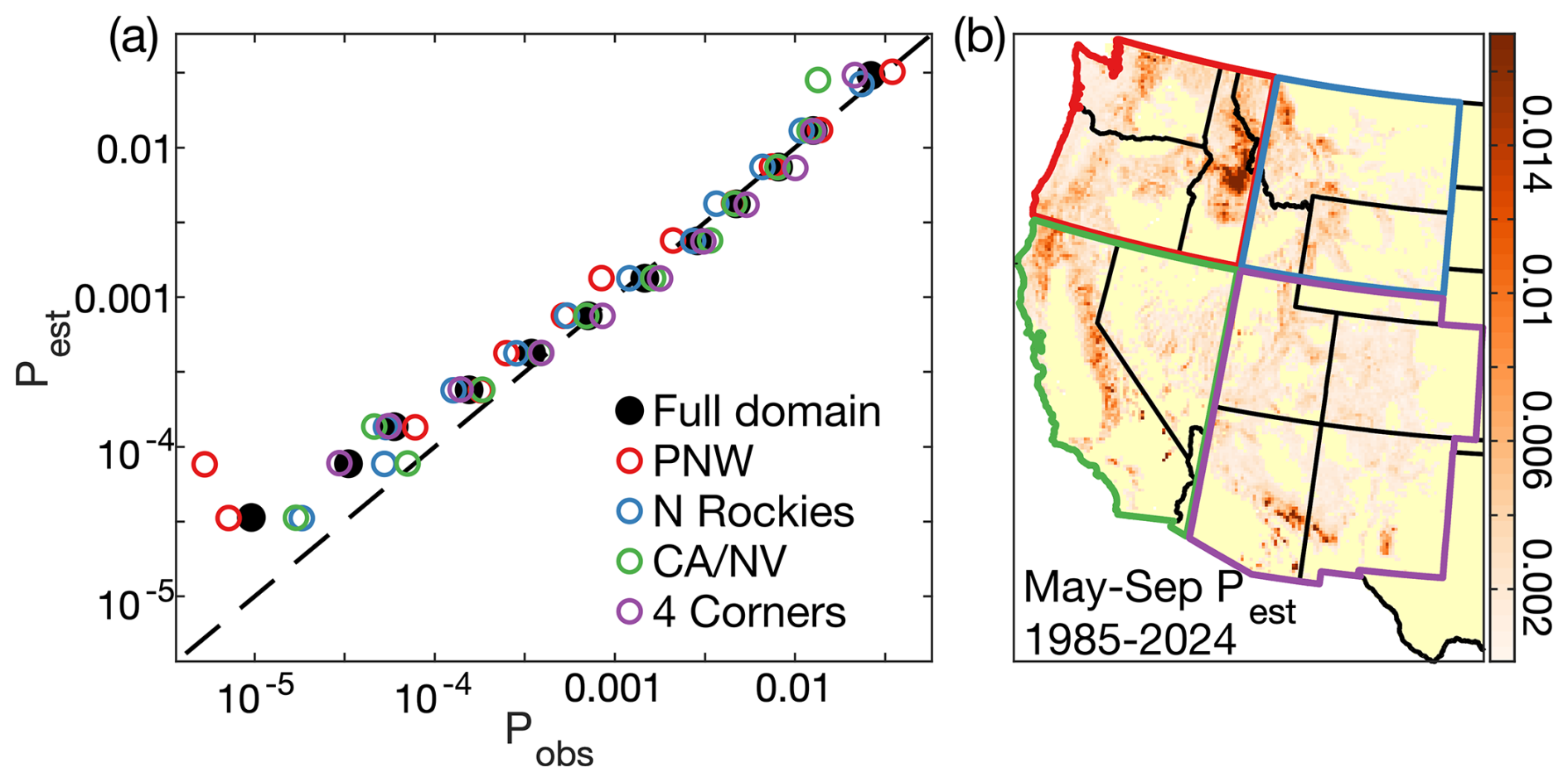
Figure 6 Fire probability estimates. (a) Mean observed and estimated probabilities of grid-months with ≥1 fire (P_obs and P_est, respectively) within each of 12 bins of P_est. Y axis values correspond to the mean P_est within each bin. Filled black dots: mean simulated versus observed frequency of all grid-months in the full western US forested domain. Empty colored dots: analysis for each of the four quadrant regions mapped in panel (b). Dashed black line: 1-to-1 line. Model estimates shown on y axis to aid visual interpretation of model errors. (b) Map of modeled monthly P_est averaged over May–September 1985–2024 with boundaries of the four regions.

4.3 Modeling number of forest fires per month

Following Westerling et al. (2011), we use the modeled probability of ≥1 forest fire occurring in a grid-month (P_est) as a single predictor in a logistic regression to estimate the probability that the number of fires in a given grid-month equals or exceeds N, where N can be 1, 2, or 3. For each possible N, a logistic regression is fit using P_est from the 7394 grid-months with ≥1 forest fire. P_N is calculated as:

$$\begin{array}{}\text{(5)}& P_N=\mathrm{1}/(\mathrm{1}+e^{(-{\mathit{\beta }}_{N\mathrm{0}}-{\mathit{\beta }}_{N\mathrm{1}}{P}_{\text{est}})}),\end{array}$$

where N varies from 1–3 and the β_N values are empirically fit logistic regression coefficients associated with each value of N. By design, P_N=1 when N=1 and P_N reduces as N increases (Fig. 7). The maximum N we consider is 3 because there are very few occurrences of grid-months in the observed dataset with >3 fires. To prevent unrealistically large numbers of fires in a grid-month, P_N is not allowed to exceed the largest P_N value that was associated with N fires during model calibration.

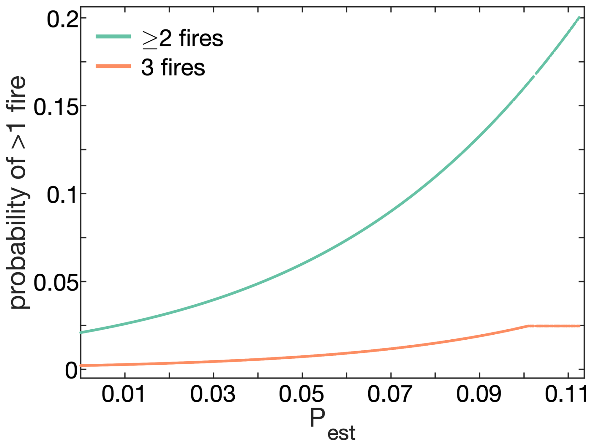
Figure 7 Probability of more than one wildfire. Given that ≥1 forest fire occurs in a given grid-month, the probability that the number of forest fires equals or exceeds 2 or 3 as a function of the modeled probability of ≥1 forest fire (P_est). The maximum number of fires in a grid-month is 3 because there are very few (<10) cases of a given grid-month having >3 fires in the observed dataset.

4.4 The forest area-burned model

To model each fire's forested area burned (A), we fit a multi-variate linear regression based on spatial (S_A), mean annual cycle (C_A), and temporal anomaly (T_A) predictor variables to estimate transformed values of A for the 7635 forest fires (Eqs. 3 and 4). Because fire sizes have a highly skewed distribution with large fires disproportionately dominating the total area burned, we statistically transform the observed values of A to quantiles and then transform the quantile values to standardized anomalies (σ) with a normal distribution (Az).

Because of the disproportionate influence of large fires on area burned, we weight Az values by the logarithm of forest area burned, linearly scaled from zero to one (Az_w). Thus we refer to the model estimating Az_w values as the Az_w model. Weights of zero (100 ha forest area burned) are reassigned the next lowest weight. To assess accuracy of the Az_w model, we use a weighted Pearson's correlation (r).

In fitting the Az_w model, we initially consider 82 potential S_A predictors, 58 potential C_A predictors, and 47 potential T_A predictors (Tables A1–A3). Because fires often burn over multiple months, the potential predictor variables for C_A and T_A include climate conditions in the month following the start date. In the second round we consider 22, 0, and 21 additional variables for S_A, C_A, and T_A, respectively. The predictor variables and curve fits selected for the Az_w model are shown in Fig. 8.

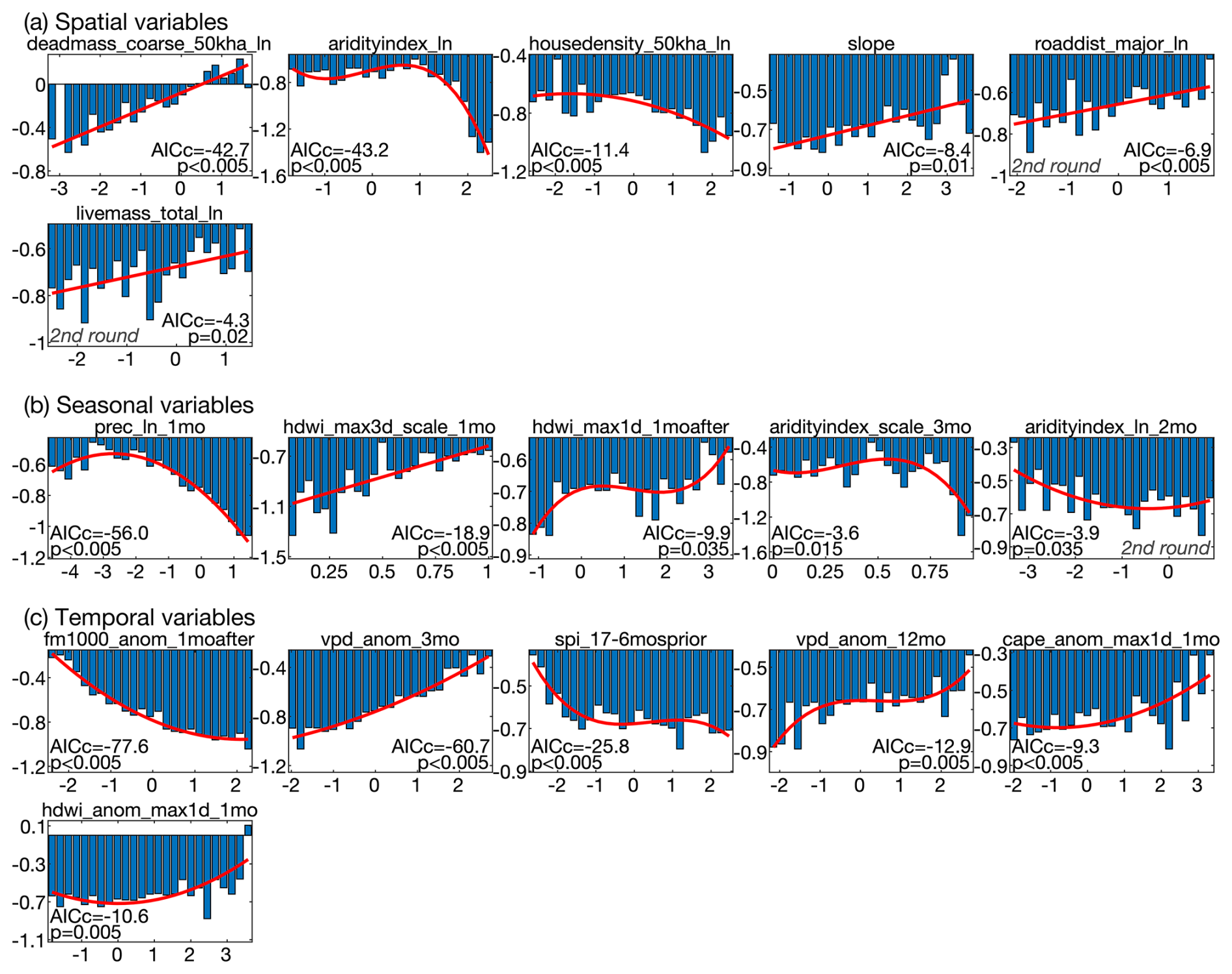
Figure 8 Predictor variables and associated curve fits in the size-weighted area burned (Az_w) model. Variables are in three categories: spatial (S_A), mean annual climate cycle (C_A), and temporal climate anomalies (T_A). Y axis values in each panel indicate residual Az_w not already accounted for prior to inclusion of that panel's predictor variable. Most residual values are negative because the weighted regression prioritizes large fires, so Az_w predictions are biased positive. Bars indicate the mean residual Az_w among observed forest fires for which the predictor variable was split into 25 evenly spaced bins. Red lines/curves indicate the linear, quadratic, or cubic fit used to approximate the response of Az_w to each predictor variable. Statistics indicate each curve fit's low-sample-size Akaike Information Criterion (AICc) and the fraction of fits that produced a more negative AICc when the values being predicted are randomly scrambled prior to binning (p). With the exception of some C predictor variables that are scaled from 0–1, units of x axis predictors are in standard-deviations from the mean. Variable names are provided above each panel and are defined in Tables A1–A3.

The variables selected for S_A indicate that large fire size is promoted where forest biomass and topographic slope are high, the long-term average climate is not too wet, and roads and population centers are far away (Fig. 8a). Variables selected for C_A indicate the annual cycle in fire size is driven by annual cycles of fuel moisture and fire weather (Fig. 8b). Variables selected for T_A indicate temporal variations in fire sizes are also dominated by fuel moisture, as represented by low FM1000, high VPD, and anomalously low prec over the prior year and a half, and high fire-weather conditions in the month of or following ignition (Fig. 8c).

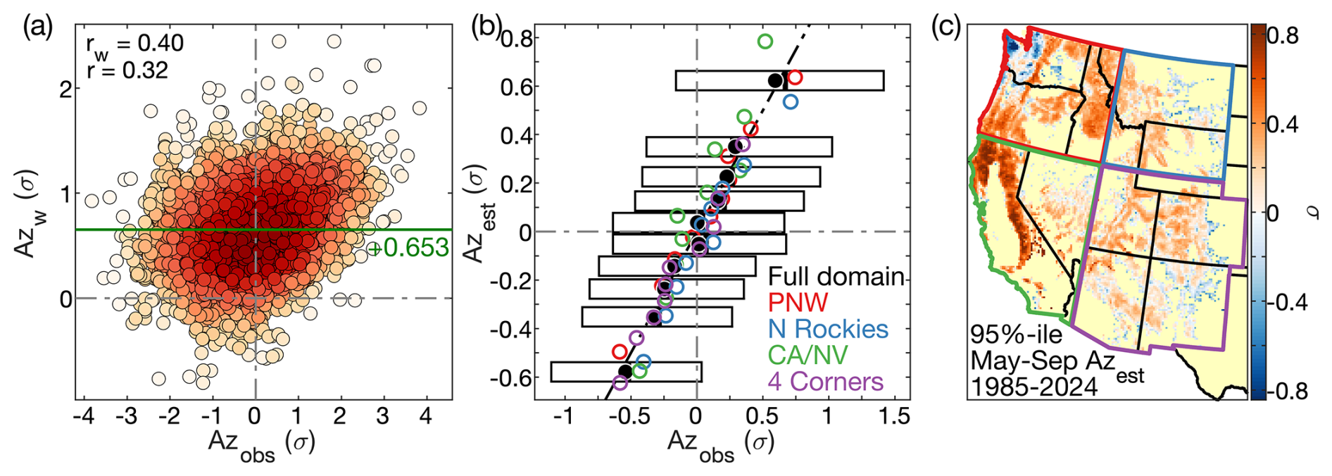
Figure 9 Fire-size estimates. Scatter plot of modeled, area-weighted normalized fire size anomalies (Az_w) versus observations (Az_obs). Redder colors indicate a higher density of sample points. The r_w and r values in the top-left correspond to the weighted and unweighted correlations between Az_obs and Az_w. The y axis position of the green vertical line and the green bias value correspond to the mean of Az_w minus Az_obs. (b) Scatter plot of binned means of modeled Az values after subtraction of the bias in Az_w (Az_est) versus the means of corresponding Az_obs values. Each black dot represents an Az_est decile for the full western US domain, with the x and y axis locations representing the mean Az_obsand Az_est values, respectively. Horizontal extents of the corresponding boxes bound the interquartile values of Az_obs and the vertical black line within each box is the median Az_obs. Colored circles show binned means of Az_est and Az_obs when the analysis was repeated for each of the four regions (PNW: Pacific Northwest, N Rockies: Northern Rockies, CA/NV: California and Nevada, 4 Corners: the four-corner states). Black diagonal dashed line: 1-to-1 line. In (a) and (b), grey vertical and horizontal dashed lines cross through the zero intercepts to aid visual interpretation. We show model estimates on the y axis to aid interpretation of model errors. (c) Map of each grid cell's 95th percentile of May–September Az_est during 1985–2024 to show geographic variability in the potential for an existing fire to grow very large.

4.4.1 Bias-correction of Az and transformation to forest area burned

Modeled values of Az_w are biased positive by an average of 0.653σ relative to observed Az (Az_obs) (Fig. 9a). This is expected because the weighted regression preferentially represents larger fires. We find no systematic tendency for the bias to vary seasonally or geographically. We apply a bias correction to calculate our model estimates of Az (Az_est) as $A{z}_{\text{est}}=A{z}_{\mathrm{w}}-\mathrm{0.653}\mathit{\sigma }$. Although our fire-size model does not account for the majority of variability among individual Az_obs values, it captures the underlying variability in mean Az_obs among larger groups of fires. For each of 10 Az_est bins, each representing an equal share of observed fires, the mean of the corresponding Az_obs values is near the mean of the Az_est values (Fig. 9b). The alignment of the colored dots around the 1-to-1 line indicates that these results generally hold at the regional scale, though with tendencies to underestimate fire sizes in N Rockies and overestimate in CA/NV. Figure 9c maps the simulated distribution of the potential for large fires, highlighting California's Sierra Nevada and Coast Range and the eastern Cascades as particularly conducive to large forest fires.

4.5 Accounting for stochastic variability

Across the western US and within the four regional quadrants, interannual variations in modeled total P and mean Az generally correlate well with observations, but simulated interannual variability is systematically muted relative to observations (Fig. 10). This is expected, as the occurrences and sizes of individual fires are highly stochastic. For more realistic representation of variability in our simulations of fire occurrences and sizes, we add semi-random variability to each modeled value of P_est and Az_est. The distributions of random variations are constrained empirically by the distributions of errors in P_est and Az_est.

Figure 10 Interannual variability. Scatter plots of annual modeled versus observed forest-fire probability (P) and normalized fire-size anomalies (Az) for the western US and each of the four quadrant regions, 1985–2024. (a–e) Modeled annual sum of P across all grid-months (ΣP_est) versus observed annual sum of grid-months with ≥1 forest fire (ΣP_obs). (f–j) Modeled annual means of Az (Az_est) corresponding to the grid-months of the observed fires versus observed annual means of Az (Az_obs). Diagonal dashed lines are 1-to-1 lines. Model estimates shown on y-axes to aid interpretation of model errors. Correlation (r) indicates Pearson's correlation between observed and modeled time series. The $\mathit{\sigma }y/\mathit{\sigma }x$ values express the standard deviation of the modeled time series as a percentage of the standard deviation of the observed time series.

4.5.1 Stochastic variations in fire probability

The distribution of uncertainty around any value of P_est is difficult to characterize because fire probability in a given grid-month can only be observed as binary, and errors in P_est can only be assessed by comparing mean values of P_est to P_obs across many grid-months. However, quantification of error in P_est averaged across many grid-months does not provide direct guidance as to the distribution of errors surrounding any single grid-month's P_est value. In exploratory analysis we found that the distribution of P_est uncertainty does not scale predictably as a function of P_est (e.g., errors are not systematically larger for larger P_est values) so we include stochasticity in our modeling of P by simply adjusting P_est with observed sequences of regionally averaged errors.

To identify regions where temporal variability in P_est is relatively coherent, we perform a rotated principal components analysis (PCA) on monthly regional errors. Initially, we divide our western US forested study domain into 64 regions based on the map of coterminous US pyromes from Short et al. (2020). To reduce the number of regions, we merge each of the 59 pyromes that averaged fewer than seven fires per year during 1985–2024 with the nearest pyrome, producing 10 forested regions with adequate fire frequencies for characterization of monthly error in P_est. For each region we calculate monthly sums of P_est and P_obs, calculate 3 month running means centered on the middle month (P_est3 and P_obs3) to reduce the effects of extreme P_obs outliers, and define the monthly error (P_error) as $P_{\text{obs3}}/P_{\text{est3}}$. We then perform a PCA on the 10 monthly time series of P_error, and retain the five principal components (PCs) with eigenvalues ≥1 as distinct modes of variability. The loadings associated with these PCs are rotated using the varimax method and multiplied against P_error to reproject the original P_error variance onto the five new rotated PC time series (PCr). The 10 original pyrome groups are combined into five new groups of relatively coherent P_error variability based on correlation between P_error and PCr (Fig. 11).

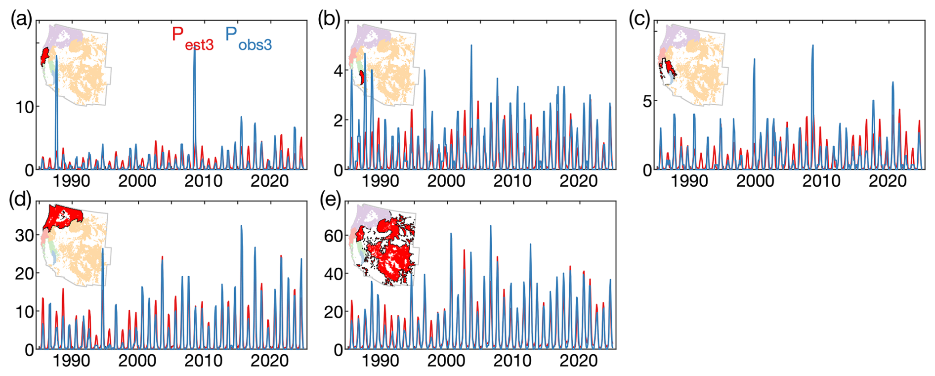
Figure 11 Intra-annual error in modeled fire probability by pyrome group. Time series of 3 month running means of the modeled (red; P_est3) and observed (blue; P_obs3) monthly sums of grid cells with ≥1 forest fire in each of five pyrome groups. Each group is composed of a group of pyromes (Short et al., 2020) with similar time series of monthly error in modeled fire probability ($P_{\text{error}}=P_{\text{obs3}}/P_{\text{est3}}$). In each panel, the red area in the map indicates the pyrome group represented by the time series and the other groups are infilled with lighter colors.

To include stochastic variability in our model simulations, we calculate an adjusted version of P_est (P_estadj) by multiplying each simulated calendar year of P_est values by a randomly drawn year of P_error from the 40 year model calibration period, where each month's map of P_error represents the regions shown in Fig. 11 (to avoid extreme values we bound P_error between 0.33 and 3). This approach preserves realistic P_error autocorrelation both spatially and between months. To demonstrate the effectiveness of this approach at eliminating the bias toward too little temporal variability in P_est (shown previously in Fig. 10a–e), we produce a 1000-member ensemble of P_estadj (Fig. 12). Including errors in our simulation successfully gives P_estadj (middle box plots in Fig. 12) a wider distribution than P_est (left box plots) that is generally better aligned with observations (right box plots). The percentage value above each set of box plots in Fig. 12 indicates how the median standard deviation of annual simulated sums of P_estadj compares to the observed standard deviation. These values are now closer to 100 % than was the case for P_est (compare to percentage values in Fig. 10a–e), indicating that our approach improves the realism of temporal variability in simulated P.

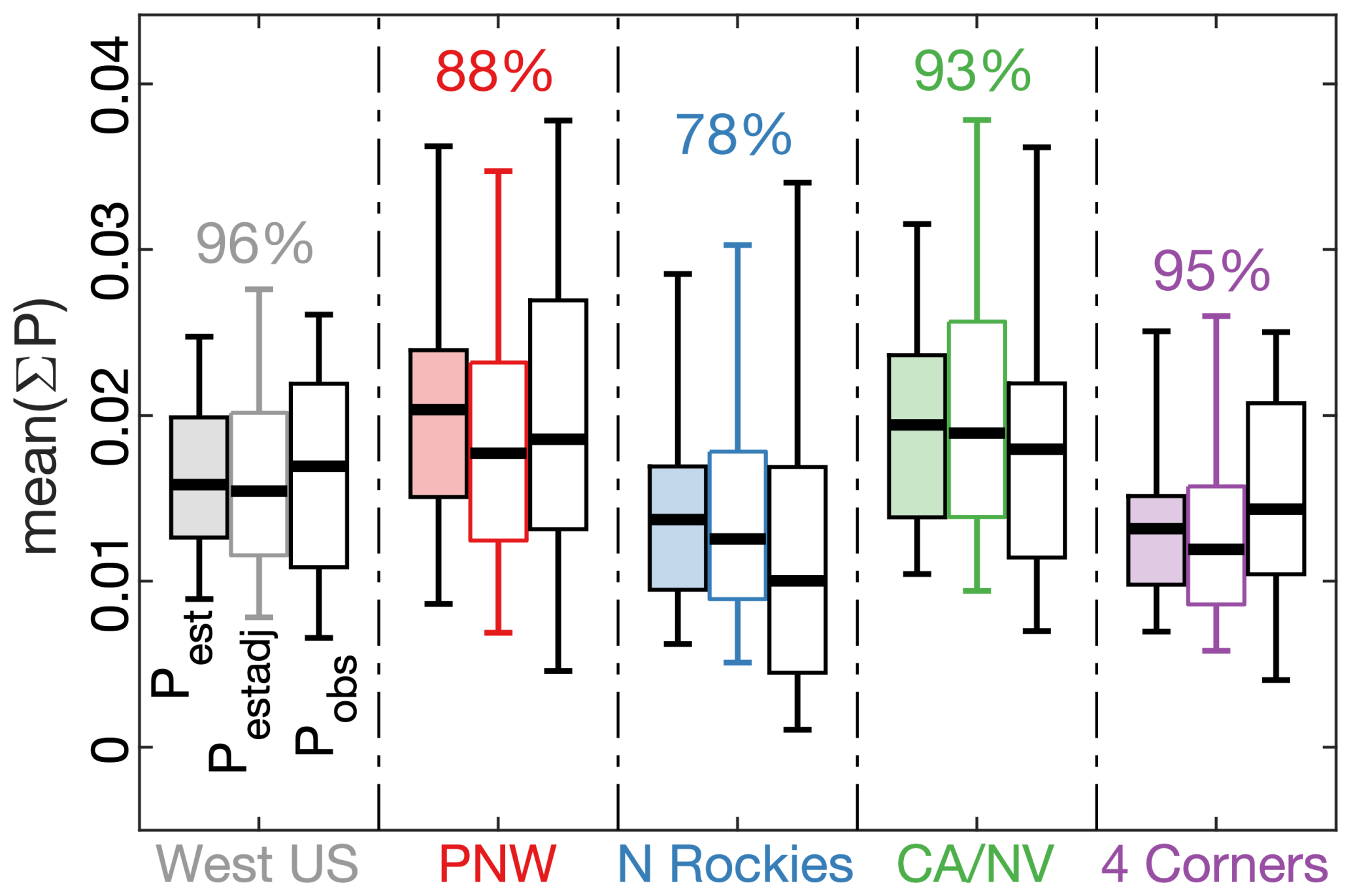
Figure 12 Distributions of modeled and observed interannual fire probability. Box plots of annual observed and modeled annual sums of the probability of ≥1 fire per month (P) averaged across all forested grid cells (mean(ΣP)) in the West US study region and the four quadrant regions. For each region, the light-colored boxplot on the left represents the distribution of the originally modeled annual time series of mean(ΣP_est): thick line is median among annual mean(ΣP_est) value, box bounds interquartiles, whiskers bound inner 90 % range. The boxplot in the middle represents the mean distribution across 1000 simulated time series of mean(ΣP_est) after adjustments to include random errors (mean(ΣP_estadj)). The white box plot on the right represents the distribution of observed sums of mean mean(ΣP) (mean(ΣP_obs)). Percentage numbers indicate the magnitude of the mean standard deviation among the 1000 simulated time series of annual ΣP_estadj relative to the standard deviation of the observed time series. Differences between these values and the percentages provided in Fig. 10a–e are due to inclusion of error in the 1000 simulations represented here. Values of annual ΣP are averaged across all grid cells for each region to reduce the influence of large regional differences in ΣP in the figure.

4.5.2 Stochastic variations in fire size

The distribution of uncertainty around estimates of Az_est is easier to assess than that of P_est because error in Az_est (εAz_est) can be quantified for each fire. In addition, εAz_est values are normally distributed and increase as a function of Az_est (Fig. 9b). As Az_est increases, the spread among corresponding εAz_est values widens and remains symmetrical. When we bin Az_est into deciles, the standard deviation among εAz_est values increases linearly with Az_est (Fig. 13). The relationship detected at the large scale of the western US also remains generally consistent at the regional scale, though the slope of the εAz_est versus Az_est relationship is higher than the west-wide mean in CA/NV and lower in N Rockies and PNW. Overall, we conclude that we can characterize the uncertainty Az_est with reasonable accuracy by simply treating it as a linear function of Az_est itself, though future work should diagnose and ideally resolve regional variations in mean εAz_est.

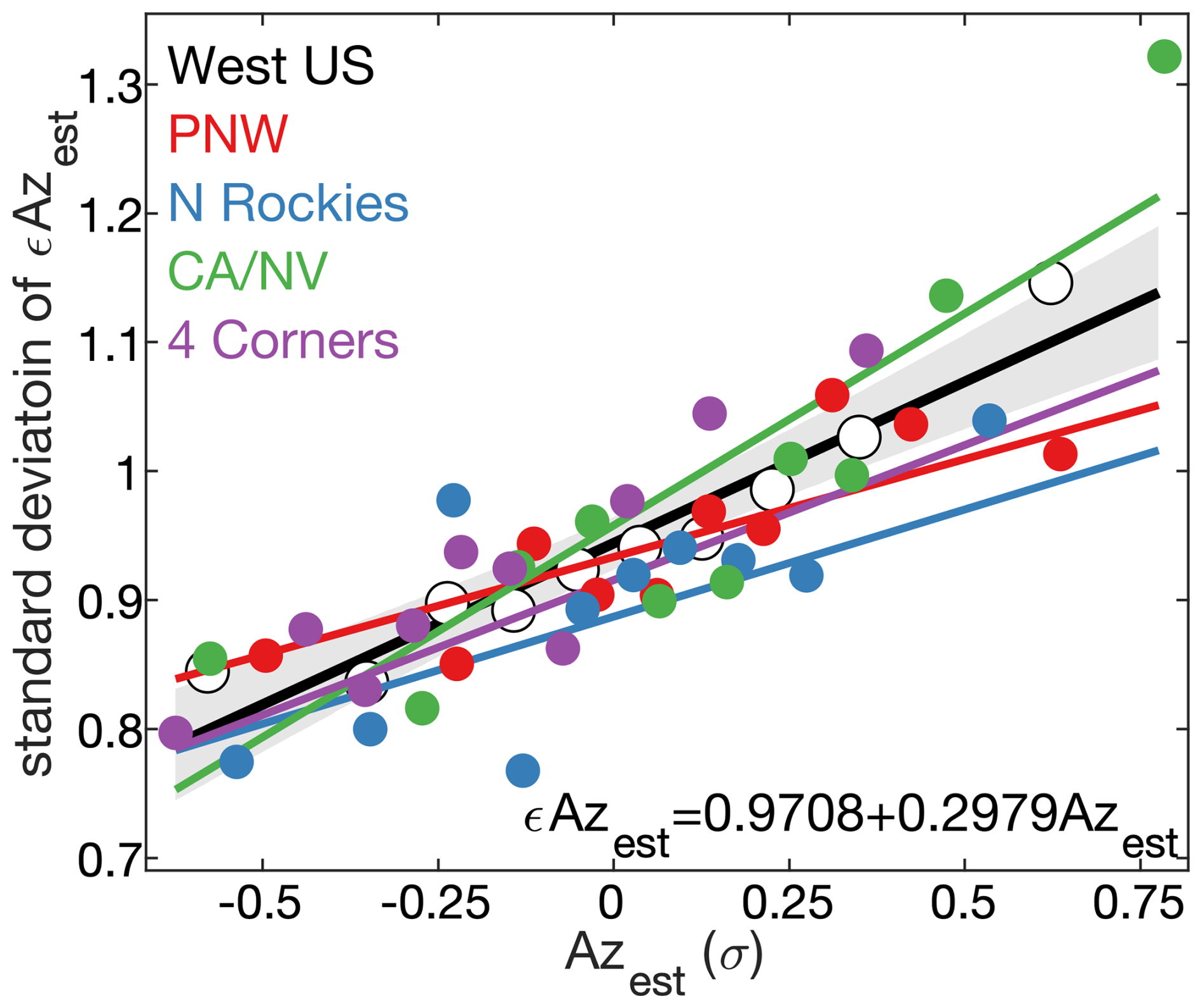
Figure 13 Variability among modeled fire-size errors. Standard deviation of error in estimates of normalized fire-size anomalies (εAz_est) as a function of Az_est for (white dots, black regression line) the entire western US forested domain as well as the four quadrant regions within: (red) Pacific Northwest (PNW), (blue) Northern Rockies (N Rockeis), (green) California and Nevada (CA/NV), and (purple) Four Corners (4 Corners). εAz_est is the observed normalized fires-size anomaly (Az_obs) minus Az_est. For each domain, Az_est values associated with observed fires are binned into deciles and, for each decile, the standard deviation of εAz_est is plotted against mean Az_est. Regression lines show the least-squares fit for each domain and the grey area bounds the 95 % confidence interval around the black regression line for the full West US domain, which corresponds to the equation at the bottom of plot.

For each simulated value of Az_est we calculate an adjusted Az estimate (Az_estadj) by adding an error value drawn from a normal distribution with a mean of zero and a standard deviation of εAz_est, where εAz_est is calculated as a linear function of Az_est following the equation in Fig. 13. Based on a 1000-member ensemble of simulated Az_estadj, this method of widening the distribution of Az_est aligns the distribution of Az_estadj with observations (Fig. 14).

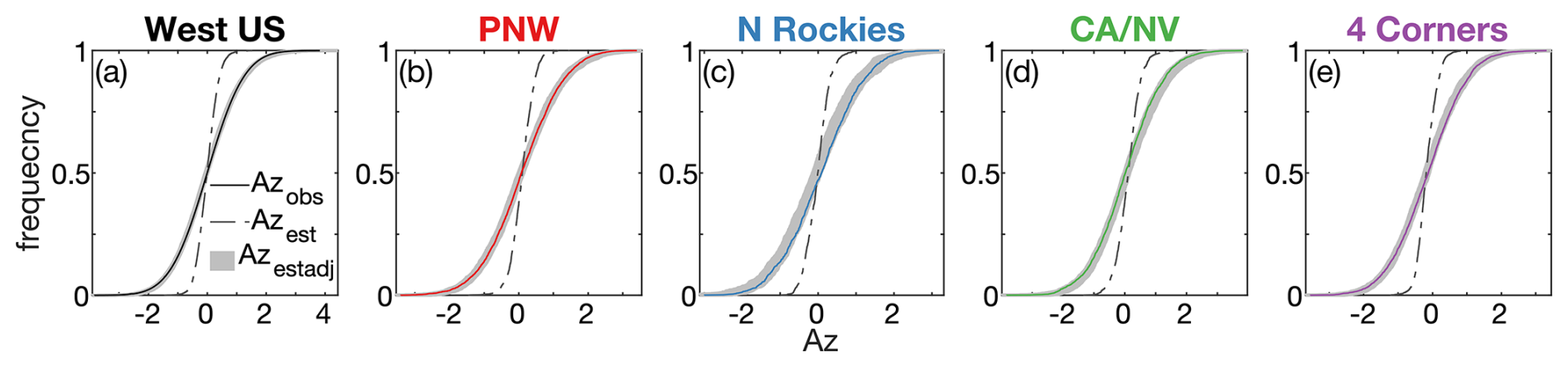
Figure 14 Effect of adding errors on the distribution of modeled fire sizes. Cumulative distribution functions of observed and modeled normalized fire-size anomalies (Az) for (a) the whole western US domain and (b–e) the quadrant regions. Thin solid lines represent observed Az (Az_obs). Dashed lines represent simulated Az before including error (Az_est). Grey areas represent 1000 simulations of Az after adjustment to include errors (Az_estadj).

Adding error to Az_est enhances the interannual variability of mean Az_estadj (Fig. 15). However, there is still a tendency toward too-little variation in Az_estadj. This is likely because errors in our estimates of Az (εAz_est) are spatially and temporally autocorrelated. We do not account for this because imposing realistic spatiotemporal covariance among εAz_est values would risk overfitting the model and reducing its interpretability.

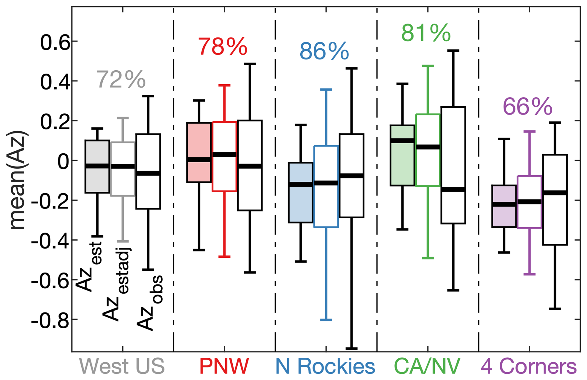
Figure 15 Distributions of modeled and observed interannual variability in mean standardized fire size. Box plots of modeled and observed annual means of normalized fire-size anomalies (Az) in the (grey) western US and (colors) four quadrant regions. For each region, the light-colored boxplot on the left represents the distribution of the originally modeled time series of mean annual Az (mean(Az_est)). The middle boxplot represents the average distribution among 1000 simulated time series of mean(Az_est) after adjustments to include random errors (mean(Az_estadj)). The white box plots on the right represent the time series of observed mean annual Az (mean(Az_obs)). Boxes bound inter quartiles, whiskers bound 5th and 95th percentiles, and thick black bars represent medians of annual values. Percentages indicate the magnitude of the mean standard deviation among the 1000 simulated time series of mean(Az_estadj) relative to the standard deviation of the time series of mean(Az_obs). Differences between these values and the percentages in Fig. 10f–j are due to inclusion of error in the 1000 simulations represented here.

4.6 Transformation of normalized fire-size anomalies to area burned

Previous work has shown that fire sizes can be effectively approximated by a positively-skewed generalized pareto (GP) distribution (Buch et al., 2023; Preisler et al., 2011; Westerling et al., 2011). We transform all values of Az_estadj to hectares of forest area burned (Agp_est) by assuming that fire sizes follow a GP distribution with the shape and scale parameters estimated from the observed forest-fire sizes. However, a comparison of the distribution of observed A (A_obs) versus the GP-transformed values calculated by back-transforming Az_obs using the empirical GP distribution parameters (Agp_obs) reveals a bias in the Agp_obs distribution because the GP is an imperfect representation of the true distribution of A_obs (Fig. 16a). We quantify the observed bias (Agp_bias_log10) as log₁₀(Agp_obs) minus log₁₀(A_obs), which we plot as a function of log₁₀(A_obs) in Fig. 16b. Much of the bias arises because the A_obs distribution has a lower bound of 100 ha (Fig. 16a), which causes the most frequent, small values of Agp_obs to be too small and the least frequent, largest values of Agp_obs to be too large.

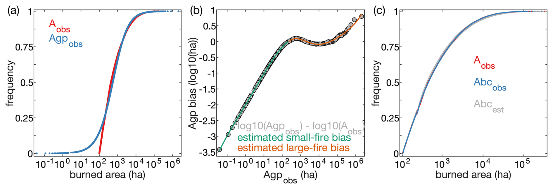
Figure 16 Bias correction of fire-size distributions. (a) Cumulative distribution function (CDF) of the observed fire sizes (red, A_obs) and the same observed fire sizes after being turned into quantiles and then back-transformed to hectares (ha) based on the observed generalized pareto (GP) distribution parameters (blue, Agp_obs). (b) Scatter plot of the bias in Agp_obs caused by the imperfect match between the actual fire-size distribution and that estimated by the GP. For small fires <223 ha, the green curve represents a 4th-order fit of the Agp bias as a function of A_obs. For larger fires, the orange curve represents a 5th-order fit. (c) Comparison of the CDFs of (red) observed fire sizes (A_obs; same as in panel a) and (blue) bias-corrected observed fire sizes (Abc_obs), where, A_obs values were first converted to normalized fire size anomalies (Az_obs), then back transformed to hectares assuming a generalized pareto distribution (Agp_obs), and finally bias corrected based on the curve fits in (b). The CDFs of A_obs and Abc_obs are overlaid on the range of CDFs produced from 1000 simulations of modeled fire sizes (grey, Abc_est), where, in each simulation, the model is used to estimate the observed fire sizes.

To reduce shortcomings of the GP distribution we bias correct such that the bias-corrected observed fire sizes (Abc_obs) take on a distribution more consistent with that of A_obs (Fig. 16c). This is done by estimating Agp_bias_log10 (Agp_bias_log10_est) as a 4th-order function of log₁₀(Agp_obs) for small fires (Agp_obs<223 ha) and as a 5th-order function of log₁₀(Agp_obs) for larger fires (Fig. 16b). Specifically, Abc_obs is calculated by subtracting Agp_bias_log10 from log₁₀(Agp_obs) and transforming the log₁₀ values back to normal, thereby restoring Abc_obs to nearly the original distribution of A_obs. In simulations, bias-corrected fire sizes (Abc_est) are calculated in the same way except Agp_bias_log10_est is calculated as a function of log₁₀(Agp_est) rather than log₁₀(Agp_obs). The grey shading behind the blue and red points in Fig. 16c represents an ensemble of 1000 simulations of Abc_est, where in each simulation we estimate all values of A_obs. The strong overlap between the grey, blue, and red CDFs in Fig. 16c indicates that our method produces realistic fire-size distributions. To prevent unrealistically large bias estimates in simulations, values of Agp_bias_log10_est should not be allowed to exceed the empirically calculated range of Agp_bias_log10 values.

4.7 Cross-validation

To assure the skill of WULFFSS is not due to overfitting, we perform temporal and spatial cross-validations. In the temporal cross validation, we retrain the models 13 times, each time withholding a period of 3–4 consecutive years such that each year in the 1985–2024 calibration period is withheld once from the training period. We then use each of the 13 models to simulate fire for the withheld periods. For the spatial cross-validation we again produce 13 models, now withholding from each calibration a contiguous region approximately 500 km×500 km in area. Each model is then used to simulate 1985–2024 fire for its withheld region. For each cross-validation approach, a full set of out-of-sample simulation outputs are produced for the western US for 1985–2024 and correlated against observations for assessment of out-of-sample skill.

5 Model Performance

The WULFFSS simulations of frequency and extent of western US forest fires are generally highly skilled. Figures 17 and 18 show observed versus simulated time series of forest-fire frequency and forest area burned at the full scale of the western US as well as for each of the four regions. See Figs. S1 and S2 in the Supplement for plots representing each of the 11 western US states. The mean of a 100-member ensemble of simulations accounts for 71 % (r=0.84) of the observed interannual variability in western US forest-fire frequency (Fig. 17a, left side). Model performance remains high out-of-sample. In the 13-fold temporal cross-validation, the cross-validated correlation between observed and ensemble-mean simulated annual fire frequency remains high at 0.81. The model performs similarly well in the 13-fold spatial cross-validation (r=0.83). WULFFSS also accurately simulates the mean annual cycle of forest-fire frequency. Correlation between the full monthly time series of observed and modeled fire frequency is strong (r≥0.90) (Fig. 17a, right side).

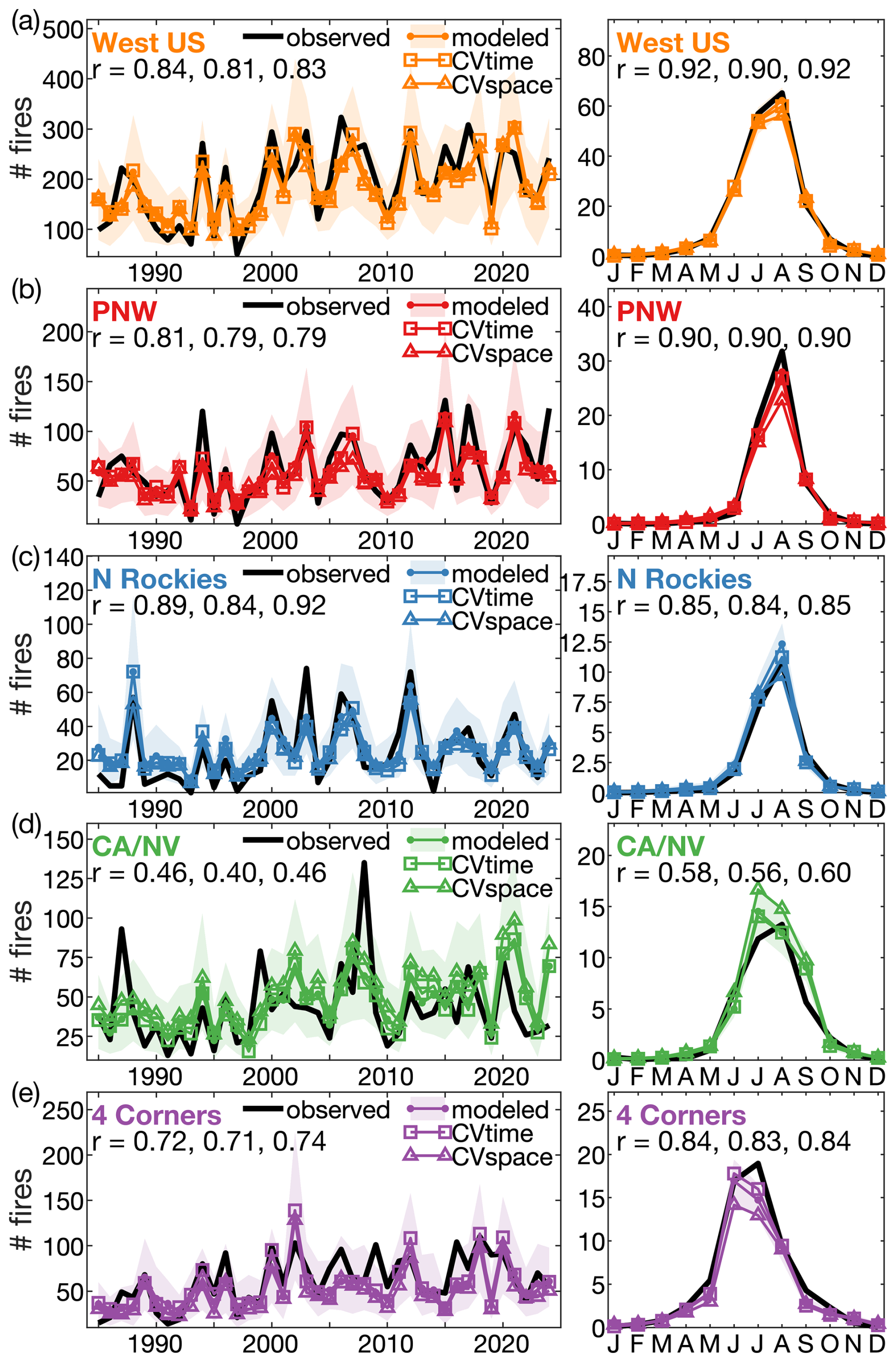
Figure 17 Modeled versus observed forest-fire frequency. Plots for (a) the western US and each of the four quadrant regions: (b) Pacific Northwest (PNW), (c) Northern Rockies (N Rockies), (d) California and Nevada (CA/NV), and (e) 4 Corners. Panels on the left show annual frequency of (black) observed and (colored) modeled forest fire. Panels on right show the mean annual cycle of monthly values. The three colored lines indicate 100-member ensemble means from (dots) the fully calibrated model, (squares) the 13-fold temporally cross-validated models (CVtime), and (triangles) the 13-fold spatially cross-validated models (CVspace). Colored shading bounds the inner 95 % of ensemble members of the fully-calibrated model. In each panel, the three correlation values (r) indicate Pearson's correlation between observations and the ensemble means from the fully calibrated model, the 13-fold CVtime models, and the 13-fold CVspace models, respectively. In the annual-cycle panels on the right, r values indicate correlation between the full observed and modeled time series of monthly fire-frequency over 1985–2024, not the mean annual cycle.

Figure 18 Modeled versus observed forest-fire area. Plots for (a) the western US and each of the four quadrant regions: (b) Pacific Northwest (PNW), (c) Northern Rockies (N Rockies), (d) California and Nevada (CA/NV), and (e) 4 Corners. Panels on the left show annual (black) observed and (colored) modeled forest area burned. Panels on right show the mean annual cycle of monthly values. The three colored lines indicate 100-member ensemble means from (dots) the fully calibrated model, (squares) the 13-fold temporally cross-validated models (CVtime), and (triangles) the 13-fold spatially cross-validated models (CVspace). Colored shading bounds the inner 95 % of ensemble members of the fully-calibrated model. In each panel, the three correlation values (r) indicate Pearson's correlation between observations and the ensemble means from the fully calibrated model, the 13-fold CVtime models, and the 13-fold CVspace models, respectively. In the annual-cycle panels on the right, r values indicate correlation between the full observed versus modeled time series of monthly forest area burned over 1985–2024, not the mean annual cycle.

The model generally performs well at the regional level, accounting for ≥62 % of variability in annual fire frequency in PNW (r≥0.79; Fig. 17b), ≥71 % in N Rockies (r≥0.84; Fig. 17c), and ≥50 % in 4 Corners (r≥0.71; Fig. 17e). The CA/NV region is an exception to the strong performance of the P model (Fig. 17d), where the ensemble-mean accounts for just 16 %–21 % of interannual fire-frequency variability (r=0.40–0.46), due mostly to large underestimates in 1987 and 2008 as well as recent overestimates in 2021–2022 and 2024. Reasons for model underperformance in CA/NV are numerous. In California (Fig. S1c), the large observed fire frequencies in 1987 and 2008 were due to anomalous dry lightning events (Kalashnikov et al., 2022), which are not adequately represented in WULFFSS. The more recent overestimates in California fire frequency may be due to increased resources for fire detection and suppression in California, increased public and corporate awareness of fire hazards, and reductions in fuel continuity due to drought and related bark-beetle outbreaks that our modeling does not capture. Nevada also contributes to the relatively low model skill in CA/NV (Fig. S1g); WULFFSS overestimates mean fire frequency by approximately 70 % in Nevada, a far larger bias than for any other state. The overestimates of fire activity in Nevada's sparse and isolated Great Basin forests suggest that our approach underestimates the ability of low biomass and vegetation connectivity to limit fire activity and/or that our DYNAFFOREST-based estimates of biomass and connectivity are too high there. In addition, while our model indicates that fire frequency is positively related to remoteness from human population (Fig. 5), ignitions may be a limiting factor in forested areas of Nevada with especially light human footprints. The model also majorly underestimates 2024 fire frequency in PNW due to a failure to capture the large number of fires in Oregon and southwest Idaho that ignited from outbreaks of dry lightning in mid and late July (Fig. S1e and i). While WULFFSS does consider long-term mean patterns of lighting activity, it does not model fire as a function of temporal variability in lightning because the only long-term lighting dataset we are aware of (from the NLDN, 1987–present) has temporal instabilities due to instrumental changes and it does not cover the full model-calibration period. While CAPE is considered to be a T variable due to its coincidence with lightning and atmospheric instability, high CAPE is also associated with precipitation, limiting its value as a proxy for dry lightning.

The model does generally well at capturing regional differences in the mean annual cycle of fire frequency (Fig. 17, right-hand panels). For example, the model correctly simulates that peak monthly fire frequency occurs in August in PNW and N Rockies but in June–July in 4 Corners (Fig. 17b–e). WULFFSS accurately simulates regional differences in the timing of onset and termination of the mean annual fire starts. On the other hand, the spatial cross-validation reveals that when training data are withheld from 4 Corners, the model underestimates fire frequencies in that region (Fig. 17e).

Model performance is also strong in terms of area burned, accounting for 86 % (r=0.93) of interannual variability in the logarithm of area burned when fully calibrated and ≥72 % (r≥0.85) in our cross-validated exercises (Fig. 18a). At the regional scale, model performance remains strong, accounting for 55 %–81 % of cross-validated variability in the four regions. The model also reproduces observed regional differences in nuanced characteristics of annual area burned. For example, the model captures the tendency for interannual burned-area variability to be dominated by extreme years in N Rockies and 4 Corners, but for interannual variability to be more evenly distributed in PNW and CA/NV (Fig. 18b–e). The model also generally captures mean annual cycles and sub-annual variations in area burned, though in CA/NV it consistently over-estimates burned areas throughout the fire season (Fig. 18d). In our state-specific analysis we find that overestimates of area burned in CA/NV are apparent in both California and Nevada, but the bias is more severe and systematic in Nevada, where WULFFSS estimates nearly four times more area burned than is observed (Fig. S2). This is the largest such bias among the 11 states, followed by Utah where estimates of area burned exceed observations by a factor of two. Consistent overestimates of area burned in Nevada and Utah, home to the relatively dry and spatially discontinuous forests of the Great Basin, further implicate fuel limitation in sparsely forested areas as a cause of error for WULFFSS.

The years with the largest errors in regional area burned are 2020 and 2024, both years when observed forest-fire extent exceeded simulations. In 2020, WULFFSS grossly underestimates area burned in PNW, and to a lesser extent in CA/NV (Fig. 18b and d). Potential contributing factors include rare lightning storms from tropical storm Fausto in August 2020, two extreme heat waves in the days to weeks immediately following the lightning storms, and overstretched suppression resources due to a high concentration of large forest fires in California and Oregon and the COVID-19 pandemic. In 2024, the large underestimate of fire frequency in PNW noted above (Fig. 17b), in Oregon and Idaho specifically (Fig. S1), translated to underestimates in total area burned (Figs. 18b and S2). However, it is likely that our observational record of area burned is biased high in 2024, as MTBS maps are not yet available for most large wildfires in that year, so the currently available maps of many of that year's largest fires do not represent within-fire spatial heterogeneity in area burned. On average, MTBS maps indicate that approximately 20 % of area within forest-fire perimeters is unburned, consistent with Meddens et al. (2016), so it is likely that our underestimate of area burned in 2024 will be lessened somewhat once MTBS data become available.

6 Discussion, strengths, and limitations

The WULFFSS simulates the monthly gridded probabilities and sizes of forest fires in the western US as a function of land cover, topography, human population, and climate. The model uses standard regression-based statistical methods, which constrains flexibility but enhances interpretability and reproducibility. The skill of our model should serve as a benchmark for more complex but methodologically opaque modeling efforts.

Our model has high skill. It simulates realistic characteristics of fire such as annual cycles, ranges of interannual variability, and fire-size distributions, as well as inter-regional differences in these characteristics. The model also has strong out-of-sample skill when reconstructing observed variations in forest-fire activity for time periods or regions withheld from the training data. This suggests that the model can reliably simulate western US forest-fire activity under idealized historical or projected conditions as long as those conditions are not far beyond those that occurred during the model training period.

The model can be easily updated as additional or improved records of observed wildfires become available. Updates and improvements of the observed fire record are enabled by the streamlined method to easily update our WUMI2024a database with newly available wildfire data (Williams et al., 2025). Our model's ability to produce trustworthy simulations under future, warmer climate scenarios will likely improve over time as more climate extremes and their effects on forest fires are observed.

A unique feature of WULFFSS is that it was developed in parallel with the forest-ecosystem model, DYNAFFOREST (Hansen et al., 2022), specifically to enable coupled simulations in which fire and forest ecosystems interact. This is important for several reasons. First, we are motivated to simulate and understand more features of fire beyond event frequency and area burned. By coupling with an ecosystem model, we can also simulate fire severity, biomass consumed, and ecosystem transitions, all crucial for anticipating changes to ecosystem health, pollution, hydrology, and terrestrial carbon storage. Further, as vegetation responds to changes in climate and fire behavior, these responses will feed back to modulate fire-climate relations. Coupling between fire and forest-ecosystem models is therefore essential for plausible projections of western US forest fire activity beyond the next couple decades.

Another feature of WULFFSS is its computational efficiency, which allows for large ensembles of simulations. A standard laptop can simulate several decades of forest fire across the western US in seconds, enabling easy generation of hundreds or thousands of simulations. This is important under climate warming because forest-fire sizes appear to respond exponentially to positive forcings such as warming and drying (Juang et al., 2022), which should cause the range of internal variability of area burned to grow under continued warming in many forested regions of the western US. Indeed, the range of modeled uncertainty in total forest-fire area is much wider in high-VPD years (Fig. 19). Although running WULFFSS while coupled within the DYNAFFOREST model is considerably more computationally expensive, DYNAFFOREST was also designed to facilitate large simulation ensembles and it is feasible to run tens of century-scale coupled simulations in the matter of days on a high-performance computer cluster. With a large ensemble of tens of historical or future coupled forest and fire simulations, one can explore the mean response (e.g., aboveground biomass consumed) to a given forcing as well as the uncertainty around the mean. Further, if an ensemble of coupled simulations is produced where each represents a plausible realization of fire effects on forest biomass, connectivity, etc., then these forest outputs can be used to force additional uncoupled WULFFSS simulations to greatly enhance the ensemble size in terms of simulated fire frequencies and burned areas.

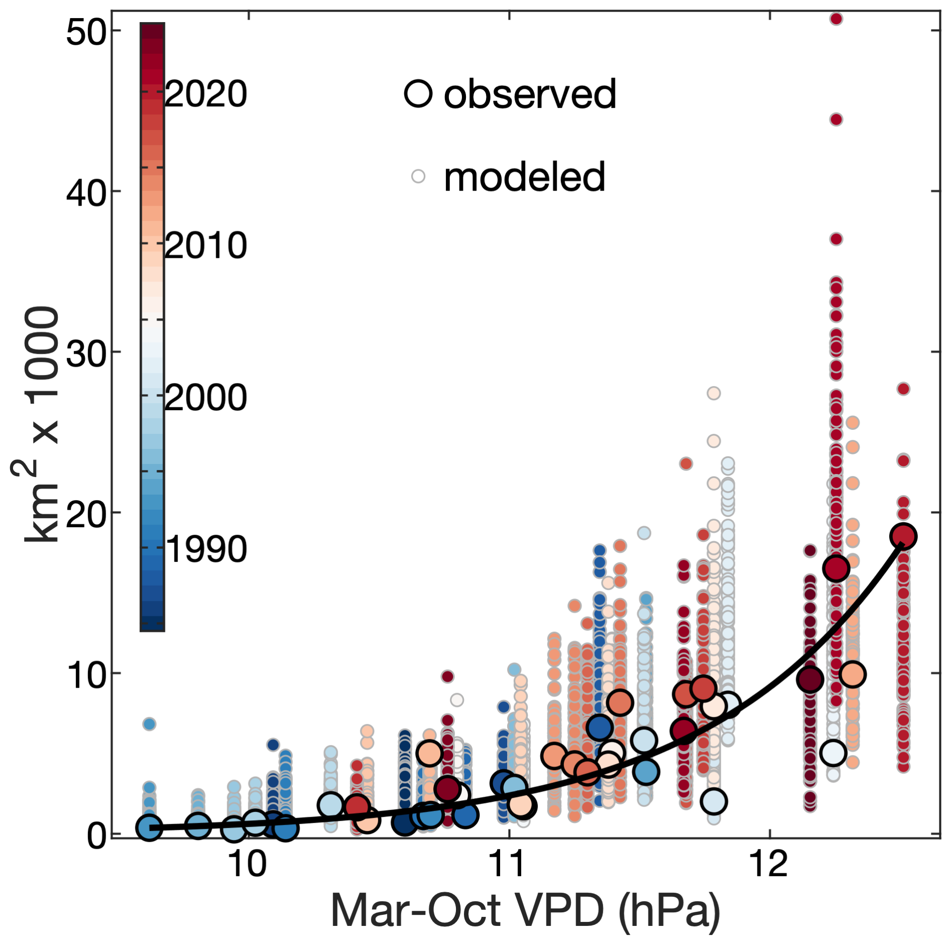
Figure 19 Western US annual forest-fire area versus March–October vapor-pressure deficit (VPD). Large dots with black outlines are observations and the black curve is the least-squares regression line relating the logarithm of observed area burned to observed VPD averaged across March–October. Small dots with grey outlines are outputs from an ensemble of 100 simulations under identical forcings, including observed climate (ensemble spread due to stochastic errors added to modeled estimates of fire probabilities and sizes). Colors correspond to years from 1985–2024.

There are a number of caveats, some of which represent opportunities for improvement while others are structural features of our approach. Opportunities include consideration of changing road networks in the past, use of road routing to more intelligently map the distance of forested areas to human population, and addition of aboveground utility lines and their ages. In addition, the model's ability to capture the effects of spatiotemporal changes in fuel characteristics is limited by a lack of spatially continuous observational data covering the four-decade model-calibration period. For example, while the model does account for the majority of the observed increase in western US annual forest-fire area since 1985, it systematically overestimates burned area in the first half of the record. One likely explanation is that the DYNAFFOREST datasets we use to parameterize WULFFSS do not fully represent fire-promoting trends in fuel amount, connectivity, and structure in recent decades. Because DYNAFFOREST is a single-cohort model, it does not explicitly simulate understory fuels, so variables related to vertical forest structure and ladder fuels are not currently considered by WULFFSS. As spatially continuous remotely sensed fuels datasets, which are so far only available for smaller regions (Hudak et al., 2020), become available across the western US, this will almost certainly improve our ability to simulate historical probability and size.

Another limitation is that WULFFSS and DYNAFFOREST do not explicitly represent non-forest vegetation. DYNAFFOREST assumes non-forest is grass and shrub, but does not explicitly simulate grass and shrub growth and decomposition. Representation of non-forest fuel dynamics would likely improve our ability to simulate fire events, particularly near the dry edges of forests and when and where simulated forest biomass is relatively sparse. This limitation appears most clearly in our simulation of fire in the isolated forests atop the narrow and arid mountain ranges of the Great Basin. In Nevada, for example, WULFFSS overestimates fire frequency by 70 % and area burned by a factor of four. In addition to limitations caused by our current lack of representation of non-forest fuel dynamics, overestimates of Great Basin fire activity are also probably promoted by positive biases in our DYNAFFOREST-simulated maps of forest biomass and connectivity in the Great Basin region. This further motivates the need for spatially continuous maps of observed vegetation biomass across the western US that cover the time period of 1980s to near present at timesteps of annual or finer, which could be used as forcings in WULFFSS simulations of the observational period and to improve vegetation ecosystem models such as DYNAFFOREST.

Likewise, more mechanistic consideration of fuel-moisture dynamics would improve the realism of WULFFSS. In the current parameterization, we mechanistically model snowpack and allow this to affect our calculation of dead fuel moisture, but the NFDRS formulations we use to estimate dead fuel moisture are relatively simple and non-mechanistic. Live fuel moisture would likely improve model skill beyond the skill yielded from our estimates of dead moisture (Rao et al., 2023), but our current approach instead relies on hydroclimate predictors to implicitly represent live fuel moisture. More thoroughly representing the complexity of moisture dynamics in an internally consistent framework that can be coupled with our ecosystem simulations would likely enhance the skill of WULFFSS. That said, fuel-moisture simulations are challenging due to the limited availability of ground-truth measurements across the complexity of fuel moisture dynamics related to species, fuel sizes, types, ages, soil type and geology, rooting depth, position within the vertical profile of the forest, stand density, and live versus dead status.

Another opportunity for improvement is to explicitly simulate fire spread. Currently, WULFFSS only estimates the final forest area burned by each simulated fire. When coupled within DYNAFFOREST, the ignition of a given simulated fire is assigned to a random 1 km forested grid cell within the 12 km grid cell of WULFFSS and the fire spirals through adjoining or nearby forested cells until the pre-determined fire size is achieved or no nearby forested cells remain. Future improvements to WULFFSS should include estimating ignition location at sub-12 km resolution and modeling fire spread while maintaining computational efficiency. For example, WULFFSS could make probabilistic determinations of sub-grid ignition location, sub-month ignition date, fire-spread duration, and daily spread rate and direction. Related to processes affecting fire spread, with the exception of our consideration of CAPE to represent likelihood for lightning or plume development, we currently only rely on surface climate to represent potential for rapid fire spread. Future work should consider how fire spread is linked to three-dimensional atmospheric dynamics.

A limitation to essentially all fire models that operate across large areas, especially statistical models like WULFFSS, is that the observations used for model parameterization inherently reflect the impacts of modern society. These impacts include non-lightning ignitions and restricted fire sizes due to suppression, as well as the indirect effects of humans on fuels (e.g., fuel accumulation due to fire suppression) and climate. Future improvements should include distinguishing human- versus lightning-caused ignitions. More challenging is to estimate fire sizes in the absence of suppression or under changes to suppression practices. The North American Fire-Scar Network, a database of historical fire scars in trees (Margolis et al., 2022), could provide guidance as to how simulated fire sizes could be adjusted to represent a fire regime with little or no suppression.

However, spatiotemporal differences in human behavior cause uncertainty in WULFFSS, even in the observed period. In 2020, for example, the observed area burned in the western US was on the upper fringe of values simulated by WULFFSS (Fig. 18). Interestingly, WULFFSS accurately simulates fire frequency in 2020, but systematically underestimates 2020 fire sizes in CA/NV and PNW. A likely explanation is that, when a rare summertime lightning event coincided with hot and dry conditions to produce widespread wildfire activity, coupled with the COVID-19 pandemic, suppression efforts had difficulty keeping up. If human activities related to ignitions or suppression change in the future (e.g., California's new ALERTCalifornia camera network instantaneously identifies fires across the vast majority of the state; https://alertcalifornia.org, last access: 30 December 2025), then the WULFFSS model in its current formulation will lose accuracy. Variables more directly related to suppression capacity than population and road density may be helpful in future modelling efforts. Notably, our consideration of annual maps of gross domestic product, a variable used in some earth-system modeling schemes to serve as a proxy for suppression capacity (Li et al., 2024a), did not contribute to model skill. Federal suppression resources may make up for much of the regional variability in wealth. Finer-scale features such as distance to the nearest fire station or aircraft availability for aerial firefighting may prove valuable in future efforts.

WULFFSS does not capture the important contributions of dry-lightning events, particularly near the west coast where lightning is relatively rare and thus a single anomalous event can cause a large increase in annual fire frequency and area burned. For example, the very high fire counts in CA/NV in 1987 and 2008 and in PNW in 2024 were due in part to anomalous outbreaks of dry lighting. Temporal variations in lightning frequency are not currently used as predictors in WULFFSS because we are not aware of an observational lightning dataset that spans our full model-calibration period and is not free of temporal inconsistencies due to changes in observational methods. Ideally, lightning would be a variable that can be modelled based on meteorological data, allowing lightning to force model simulations representing time periods or idealized scenarios beyond the 1985–2024 period of focus here. While lightning frequency has been shown previously to be well correlated to CAPE multiplied by precipitation total (Romps et al., 2018), the likelihood of ignition from lightning is substantially reduced if it coincides with precipitation. We thus consider CAPE on its own as a potential proxy for dry lightning potential, but ultimately CAPE was not selected by our fire-probability model. Future efforts to identify meteorological proxies for dry-lightning potential would likely enhance our model's simulations of fire-frequency extremes.

Finally, in developing the WULFFSS we made the unconventional choice to bin separately the effects of predictors whose variance lies primarily in one of three domains: spatial, mean annual climate cycle, and lower-frequency temporal variability of climate. Our reasoning was that spatial variations in the potential for fires to ignite and spread modulate the fire-promoting potency of temporal variations in weather and climate. For example, climate conditions that dry out fuels are more likely to translate to heighted potential for wildfire in areas where fuels and potential ignition sources are abundant. However, the logic behind separating out the effects of climate into those driven by the mean annual cycle versus lower-frequency anomalies is debatable. On one hand, there is probably not a major difference between the mechanisms that cause wildfire activity to exhibit an annual cycle versus those that cause interannual variability, so allowing the model to represent these sources of variability as separate mechanisms is not ideal. On the other hand, many climate variables share a similar annual cycle and climatological differences between opposing ends of the annual cycle are often much larger than the range of climatic variability that distinguishes years of high versus low fire potential. Thus, a statistical fire model trained on both intra- and inter-annual climate variability simultaneously risks over-representing variables that best correlate with the mean annual cycle in fire occurrences or sizes (e.g., solar intensity) but are not dominant drivers of interannual variability. That bias would dampen lower-frequency variability in simulated fire activity and inhibit the diagnosis of past and future changes in western US forest-fire activity. High-quality data on live and dead fuel moistures could ameliorate the need to simulate the drivers of intra- and inter-annual variability separately by reducing our reliance on the multiple and covarying climate predictors that we currently use to represent the water balance (e.g., precipitation total, wet-day frequency, FM1000, and VPD over multiple time scales).

7 Conclusions

We developed a monthly stochastic forest-fire model, the WULFFSS, for the western US that operates on a 12 km resolution grid and simulates the probabilities and sizes of large forest fires (≥1 km² forest area burned). Predictor variables include vegetation characteristics, topography, human population, and climate. When trained with observed data, WULFFSS reliably reproduces observed spatiotemporal variations in fire occurrence and area burned. Model performance remains high when tested in cross-validations against out-of-sample observations. The complex nature of wildfire and its nonlinear responses to many interacting variables has motivated efforts to model wildfire with machine-learning techniques (Wang et al., 2021; Brown et al., 2023; Buch et al., 2023; Li et al., 2024b). These efforts are valuable, but should not wholly replace models such as ours that use conventional statistical methods that are generally more straight-forward to interpret and understandable for more people. Models developed using relatively simple methods provide value by establishing baselines against which machine-learning efforts can be compared. Further, it is increasingly evident that fire needs to be simulated within ecosystem and hydrological models in order for plausible simulations of future changes to ecosystem composition, terrestrial carbon storage, snowpack, and streamflow (Bowman et al., 2009; Anderegg et al., 2022; Koshkin et al., 2022; Williams et al., 2022). Statistical modeling approaches therefore remain valuable in wildfire science, as ecosystem and land-surface modeling groups may be hesitant to adopt a machine-learning based fire model that is difficult to implement or explain. In the case of WULFFSS, we developed it to be coupled with our western US dynamical forest-ecosystem model, DYNAFFOREST (Hansen et al., 2022). With WULFFSS and DYNAFFOREST, we can efficiently perform large ensembles of tens or hundreds of century-scale simulations of the coupled forest and wildfire processes across the western US. With this coupled approach we can quantitatively address questions about the relative contributions of human-caused climate change and fire-management practices to recent increases in forest-fire activity, how these contributions have varied geographically, and how forest ecosystems and western US fire regimes may evolve under future climate change. Further, fire research is often heavily focused on fire frequency and size because these metrics are easiest to observe. Coupling WULFFSS with a forest-ecosystem model will allow for simulation of other important fire metrics such as severity and biomass loss. Finally, WULFFSS is a long-term, evolving project. Improvements will include simulation of fire spread, simulation of multiple tree cohorts to simulate ladder-fuel effects, simulation of grass and shrub communities to better represent fuel continuity, distinguishing between human versus natural fire ignitions, and explicit simulation of human effects on ignitions and fire sizes via suppression.

Appendix A

Table A1 Potential predictor variables dominated by spatial variability. “P model use” indicates whether the sign of the effect of a given variable on fire probability had to be positive (+) or negative (–), or if a given variable was not considered as a potential predictor of fire probability. “Size model use” is same as “P model use” but for the fire-size model. “Round 2 only” indicates variables (×) only considered in the second round of model fitting. Variables with “in50kha” represent average conditions within a surrounding area of approximately 50 000 ha (a 23 km×23 km box). Variables with “log10” are log-transformed. See Table S1 in the Supplement for variable descriptions.

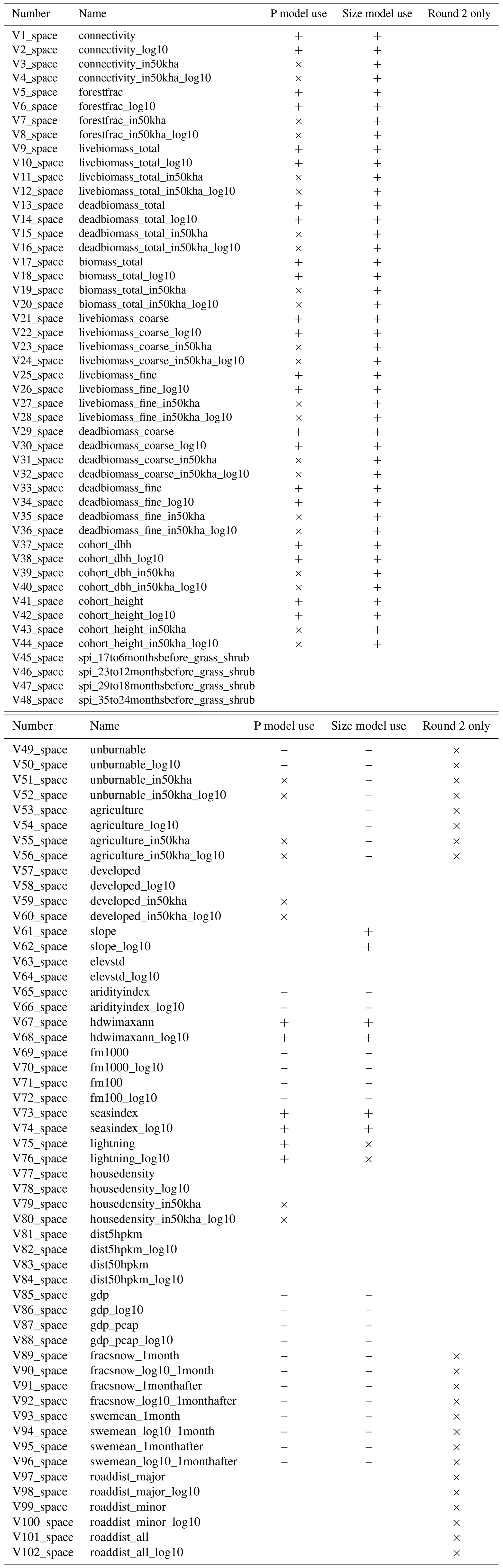
Table A2 As in Table A1 but potential predictor variables representing the mean annual climate cycle. Climate predictors with “mean” indicate the mean annual cycle of monthly values during the model calibration period (1985–2024). Variables with “mean_scaled” are mean annual cycles linearly scaled between zero for the annual minimum and 1 for the annual maximum. Durations at the end of variable names (e.g., “3month”) indicate that monthly values are averaged with a moving window of the indicated duration prior to calculation of the annual cycle, with the moving window ending in the month for which the average is assigned (e.g., the 3 month average assigned to March is calculated across January–March). Variables with “1monthafter” represent mean climate of the next month (e.g., the mean annual cycle value assigned to January represents that of February). See Table S2 in the Supplement for variable descriptions.

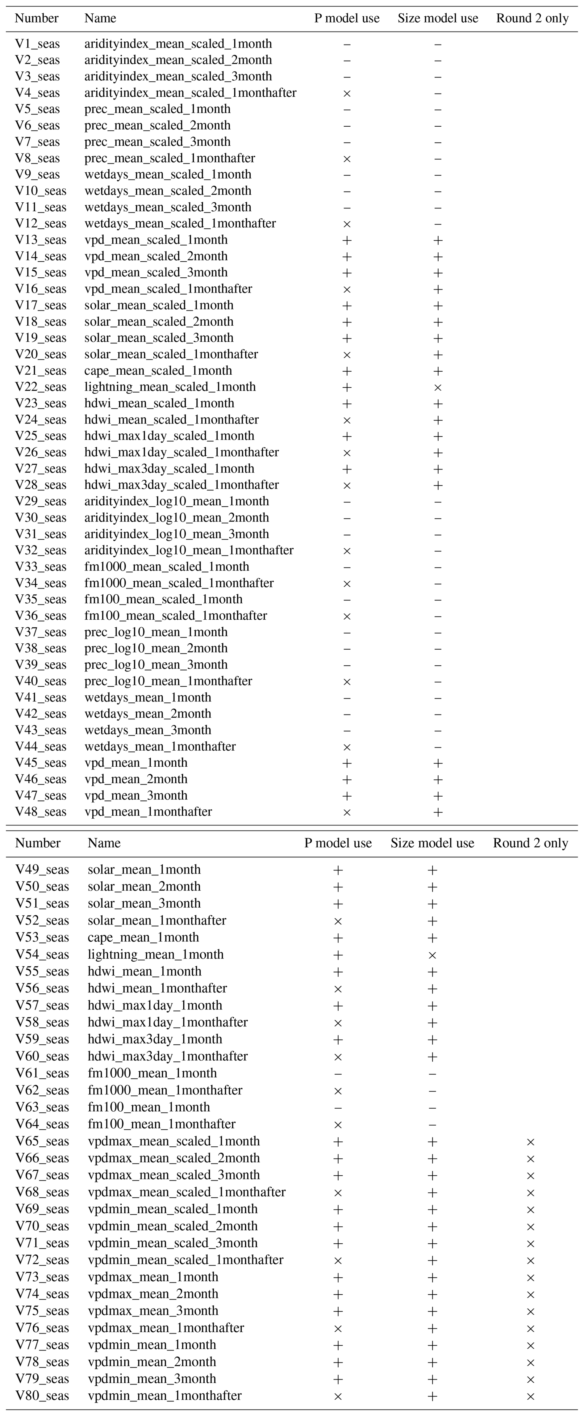
Table A3 As in Table A1 but potential predictor variables representing temporal variability at timescales beyond the mean annual cycle. Durations at the end of variable names (e.g., “3month”) indicate that monthly values are averaged with a moving window of the indicated duration prior to calculation of anomalies, with the moving window ending in the month for which the average is assigned (e.g., the 3 month average assigned to March is calculated across January–March). Variables with “1monthafter” represent mean climate of the next month (e.g., the mean annual cycle value assigned to January represents that of February). Variables with “anom” are standardized such that, for each of the 12 months, the mean is zero and standard deviation is 1 during the model calibration period of 1985–2024. See Table S3 in the Supplement for variable descriptions.