Deploying machine learning components coupled to Earth System Models with OASIS3-MCT (v6) and Eophis (v1.1)

The integration of machine learning (ML) components into Earth System Models (ESMs) holds significant potential for improving climate simulations, but it is often constrained by challenges related to interoperability, reproducibility, and computational efficiency. This paper presents a novel coupler-based approach that combines the OASIS3-MCT coupling library with Eophis, a high-performance Python library, to seamlessly deploy ML components in ESMs. By leveraging OASIS3-MCT’s robust communication infrastructure, Eophis abstracts the technical complexities of coupling, enabling users to integrate Python-based ML models or analytical parameterizations into geophysical simulations. Eophis provides a modular interface for defining data exchanges, synchronizing time steps, and supporting parallel communications, including advanced features such as halo construction for Convolutional Neural Networks and hybrid CPU/GPU execution. We evaluate this framework by coupling the NEMO4 ocean model with both ML-based and analytical parameterizations, demonstrating scalability, asynchronous execution, and flexible resource allocation. Benchmarking results show that this approach allows for deploying Python scripts in NEMO without affecting time-to-solution, provided extra computing resources are adequately allocated. The combination of OASIS3-MCT and Eophis offers a user-friendly solution for hybrid modelling, which facilitates the integration of ML components into ESM workflows.

By lowering the barrier to hybrid modeling, this work facilitates the integration of ML components into ESM workflows. The combination of OASIS3-MCT and Eophis offers a practical solution for bridging the gap between ML and climate modeling, supporting innovation in Earth system science while maintaining reproducibility and ease of use.

1 Introduction

Application of machine learning (ML) to scientific computing has grown rapidly, giving rise to a new interdisciplinary field commonly referred to as Scientific Machine Learning (SciML) (Baker et al., 2019; Karniadakis et al., 2021; Keith et al., 2025). This field encompasses a wide range of applications, including the design of numerical solvers, subgrid parameterizations, algorithms for inverse problems, surrogate models, emulators, data assimilation and uncertainty quantification. These advances are reshaping how scientists approach modelling and simulation in many areas of computational science. Application of SciML to computational geosciences has also grown rapidly, in particular in the context of Earth System modelling. Given their computational cost and structural complexity, Earth System Models (ESMs), which aim to simulate the time evolution of climate variables in response to diverse forcings, indeed stand to benefit significantly from ML techniques.

The concept of hybrid Earth System Models, combining data-driven and physics-based components, has been proposed for improving long-term projections of Earth's physical climate (Reichstein et al., 2019; Irrgang et al., 2021; Zanna et al., 2025). While their physics-based components implement known physical laws, their data-driven components are trained, based on observational or simulated data (Watt-Meyer et al., 2024), with the aim of improving the skill and reducing the cost of the resulting ESM. The formulation of subgrid parameterizations and bias correction schemes has been tackled with such approaches, which have now been tested with most components of ESMs, including the atmosphere, ocean, land surface, and cryosphere (Beucler, 2025). While open questions remain concerning hybrid models' ability to generalize outside the range of their training data, the modular nature of ML components offers a compelling path toward making ESMs more adaptable and extensible. In practice, however, integrating trainable components into current generation ESMs remains a complex task. A primary difficulty lies in bridging the gap between the ML and climate modelling communities, which typically operate in different software environments and follow different development paradigms. This has raised important concerns related to computational efficiency, ease of deployment, code maintainability, and scientific reproducibility. Over the years, several integration strategies have been proposed. These range from implementing neural networks directly in Fortran, to interfacing with ML libraries via Python/C bindings, to using C++ wrappers or high-level APIs that abstract away the underlying complexity. Each approach carries trade-offs in terms of performance, portability, and ease of use. In this work, we propose a new approach to address these challenges by leveraging an already well-integrated component in many current-generation ESMs: their coupler. We introduce a new high-performance library that simplifies the deployment of ML components in ESMs which use the OASIS3-MCT coupling library (Craig et al., 2017). Our library is designed to be modular, efficient, and compatible with existing ESM infrastructure. We demonstrate its capabilities through a series of performance benchmarks and functional comparisons against alternative integration strategies. Although the test cases in this study are limited to the NEMO ocean model, the proposed approach is designed to be applicable to other global¹ and regional² ESM components equipped with OASIS3-MCT. Our results highlight not only the computational advantages of the proposed approach, but also its potential to streamline the adoption of ML components in operational ESM workflows.

The paper is organized as follows. In Sect. 2, we present the existing solutions to implement ML components in ESMs and our arguments for using couplers as an interface. Then, we propose and present a Python library named Eophis that aims to overcome limitations and difficulties in setting up coupling between ESMs and ML components in Sect. 3. The computational performance of Eophis is evaluated in a series of test cases presented in Sect. 4. Finally, we discuss and summarize our results in Sects. 5 and 6.

2 Technological landscape of hybrid models

2.1 Existing solutions for online inference in hybrid models

In this paper, we examine software solutions that enable online inference of pre-trained machine learning (ML) components within physics-based simulation environments. Achieving this integration in practice requires dynamically updating the simulator’s state during run time based on the predictions of the ML component, thus coupling data-driven inference with the evolving physical system. This task is distinct from online learning, which entails optimizing the parameters of a ML component using a training objective that incorporates the physics-based simulator itself (Frezat et al., 2022). The latter typically necessitates the use of differentiable solvers (Shen et al., 2023; Gelbrecht et al., 2023) and falls outside the scope of the present work. A primary challenge for online inference of ML components in ESMs is bridging the heterogeneity of programming languages and hardware optimization. ML libraries and their communities predominantly use high-level, Python-native APIs, while ESMs are typically written in low-level languages like Fortran, which are optimized for high performance. Beyond the language difference, ESMs are often composed of CPU-optimized codes, whereas many ML libraries are developed for and run most efficiently on GPUs. Therefore, interfaces are essential to enable communication and data exchange between these disparate entities, allowing for a seamless integration of hybrid models.

Over the past years, several practical solutions have been tested for online inference of ML components in Fortran codes. Existing solutions can be classified into five main categories.

The first category leverages advanced features of recent Fortran versions to develop Fortran-written ML libraries. These approaches implement in Fortran some of the standard ML abstractions for constructing, training and calling neural networks (NN). This is proposed for instance by neural-fortran (Curcic, 2019), module_neural_net as part of NCAR PUMAS (ESCOMP, 2025), and Fiats (formerly inference-engine) (Rouson et al., 2025). A subcategory of approaches proposes to convert NN built and trained with Python native ML libraries into Fortran code. Fortran-Keras-Bridge (Ott et al., 2020) and FNN (Farchi et al., 2022) projects propose a collection of tools to convert Keras NN in such a way, as well as Fortran modules to load and use them. The main benefit of the above solutions is to ease the integration of ML projects in existing Fortran codes, but they require users to be experienced Fortran programmers. One other caveat is that these solutions may not systematically integrate the latest advances available in prominent ML libraries, in particular in terms of NN architectures.

The second category of solutions seeks to enable the direct invocation of ML library functions – implemented in languages other than Fortran – from within a Fortran environment. These approaches build upon the C/C++ APIs of widely used ML libraries, which provide the foundation for developing Fortran wrappers that expose their functionality within Fortran applications. PyTorch NN can be wrapped for inference by TorchClim (Fuchs et al., 2024), which provides additional layers to ease wrapping in the Community Earth System Model (CESM) framework. FTorch (Atkinson et al., 2025), TorchFort (Romero et al., 2024) and pytorch-fortran (Alexeev, 2023) are also Fortran wrappers for PyTorch NN that include training features. TensorFlow NN can be wrapped for inference by Fortran-TF-lib (Atkinson et al., 2023) and Infero (Bonannim and Quintino, 2024). The Infero wrapper also includes TensorRT and ONNX-Runtime, the latter providing interoperability with most common ML libraries.

A third category of solutions consists in calling Python scripts containing ML components from Fortran code, using C and Python bindings. These solutions eliminate the need to manipulate neural networks directly from Fortran and instead allow ML practitioners to operate within Python, the native environment for most ML development. CFFI (C Foreign Function Interface) is a library that allows Python functions to be exposed as C functions, which can then be called from Fortran through the standard Fortran-C bindings. More directly, Forpy (Rabel, 2020) and call_py_fort (Brenowitz, 2023) are two Fortran modules that enable the wrapping of Python objects and functions. With these approaches, Fortran variables are converted to Python representations and passed as arguments to functions imported from Python scripts; the returned results are then converted back to Fortran. Illustrative applications of this strategy can be found in the studies by Zhang et al. (2023a) and Arnold et al. (2024). Although these approaches offer considerable flexibility in designing bridges between Fortran codes and Python scripts, the types of Fortran variables that must be transferred to Python are typically similar across applications–most often arrays representing physical fields discretized on a fixed grid. Consequently, manually converting each variable for every new use case introduces unnecessary redundancy and can become a limiting factor in practice.

A fourth category of solutions for hybrid modelling relies on higher-level abstractions, such as couplers. Couplers are software components designed to exchange fields between different codes through Message Passing Interface (MPI) routines, often defined on different discretization grids, and therefore typically include interpolation capabilities. They are widely used in Earth System Models to integrate distinct model components – for example, facilitating the exchange of variables between ocean and atmosphere models at the sea surface. Couplers generally enforce strict rules and protocols regarding the formatting of fields to be exchanged. Developing Python APIs for couplers through Fortran/Python bindings can therefore reduce the redundancy found in previously discussed tools by leveraging the standardized interface already provided by the coupler and used in the component codes to communicate with the rest of the coupler system. In this setup, an ESM and a Python script containing ML components – each implementing a coupling interface – are executed concurrently and exchange data throughout the simulation. Coupling solutions for online inference of ML components may be custom-designed (Zhang et al., 2025; Wang et al., 2022; Zhong et al., 2023) or built upon existing libraries, such as PhyDLL (Serhani, 2023) or SmartSim (Partee et al., 2022). Couplers commonly employed in Earth System Models can also be readily adapted for this purpose, especially if they are already equipped with Python bindings. Studies by Balogh et al. (2024) and Arnold et al. (2024), respectively used the OASIS3-MCT (Craig et al., 2017) and YAC (Hanke and Redler, 2019) coupling libraries to hybridize atmospheric models with Python scripts containing ML components.

A final category of hybrid modelling solutions involves constructing Python wrappers around existing Fortran ESMs and integrating them into production workflows implemented in Python or other high-level languages. McGibbon et al. (2021) introduced such a wrapper for the NOAA FV3GFS atmospheric model, providing an interface that allows Python to advance the Fortran main loop and to retrieve or modify variables used within the Fortran code. With this approach, updating the model state using the output of a pre-trained ML component becomes straightforward, since both the ML component and the Fortran-based simulator are accessible from within the same Python environment. Wrappers for legacy models, however, are inherently model-specific and must be carefully engineered to align with the structure and requirements of the particular ESM under consideration. Interestingly, from the user’s perspective, the effort required to integrate ML components into physical models using this approach is, in practice, very similar to that involved in hybrid modelling with ESMs implemented directly in high-level languages. Several examples of hybrid models based on scalable ocean or atmosphere models implemented in Python (Häfner et al., 2021) or Julia (Silvestri et al., 2025; Klöwer et al., 2024) have indeed been implemented over recent years (Kochkov et al., 2024; Meunier et al., 2025).

Figure 1 Coupling through OASIS3-MCT with Eophis principle diagram. The Earth System Model and Eophis are executed independently. Both can exchange data through the coupling library. Eophis flexibly automates the configuration of the OASIS3-MCT Python API, and runs a generic Python environment compatible with the OASIS3-MCT usage in which any functions can be imported. In this example, the Earth System Model sends two fields named U and V to Eophis through OASIS3-MCT. These are passed as arguments to the Python function F, imported from a separate Python script, and Eophis leverages OASIS3-MCT Python API to send the result back to the Earth System Model.

2.2 The OASIS3-MCT coupling library and the Eophis library

We aim to investigate hybrid modelling strategies that are both intuitive for ML practitioners – facilitating rapid prototyping – and efficient for large-scale production applications. For this reason, we concentrate on a coupler-based approach (corresponding to the fourth category described above), as it allows heterogeneous model components to operate within distinct programming environments while requiring only minimal bindings. Our development is based on the OASIS3-MCT coupling library (Craig et al., 2017), specifically OASIS3-MCT v6 (Valcke et al., 2025). OASIS3-MCT is a middleware framework widely used in the climate modelling community. It provides Fortran, C, and Python APIs and has been integrated into several European Earth System Models. The role of OASIS3-MCT in a coupling between a Fortran ESM and a Python script can be briefly described as follows. Both components implement the OASIS3-MCT API and are executed as independent jobs. If the ESM sends a field through the OASIS3-MCT Fortran API, OASIS3-MCT will perform the MPI communications required to transfer the field from the Fortran processes to the Python processes. The field becomes available through the OASIS3-MCT Python API and can be used on the Python side. The same operation can be performed in the opposite direction, for instance to transfer a field from the Python script back to the ESM, as illustrated in Fig. 1.

Although OASIS3-MCT and coupling libraries offering similar API diversity, such as YAC, have already been employed for hybrid modelling, the practical steps to develop such couplings remain non-trivial. The heterogeneous APIs are in principle sufficient to couple a Fortran ESM with a Python script, but their design does not fully address the specific requirements of ESM-ML coupling for inference. In practice, these coupling libraries assume that all coupled components share a set of features typically implemented in ESMs: (i) a time-stepping procedure, implying time-synchronized exchanges, (ii) an internal MPI communication layer enabling optimal parallel decomposition, and (iii) autonomy in generating both the physical fields to be exchanged and the discretization grids on which they are defined. By contrast, the NN embedded in the Python script merely ingests geophysical fields produced by an existing ESM and returns inferred results. Thus, the Python script can be viewed as a standalone function, unable to generate physical data or discretization grids on its own. This design renders both the time-stepping procedure and the MPI parallelization unnecessary on the Python side, since the NN passively awaits inputs without consideration of temporal synchronization or domain decomposition. Consequently, current ESM-ML coupling applications require the user to manually reproduce and configure these missing features in the Python script in a case-specific manner. This makes the implementation process of the OASIS3-MCT Python API challenging and difficult to generalize.

The ESM-ML asymmetry leads to a second important characteristic. The passive waiting behavior of the Python script establishes a coupling pattern driven entirely by the ESM. Unlike conventional ESM-ESM coupling, where concurrent calls to the coupling library may lead to deadlock situations, exchanges here reduce to sequential back-and-forth communications initiated by the ESM. Several synchronization concerns traditionally associated with OASIS3-MCT become unnecessary in this context. Similarly, the absence of grid generation on the Python side makes the interpolation capabilities of the coupling library superfluous, as the Python script is required to receive fields directly on the native Fortran discretization. These apparent simplifications make several classical coupling features unnecessary in principle. Yet they still have to be configured, adding avoidable complexity.

Finally, even once the OASIS3-MCT API is properly implemented in the Python script with the necessary features, additional work is needed to configure the OASIS3-MCT Python interface. This includes defining the computational grid on which the exchanged fields are discretized, registering the fields as variables to be sent or received through OASIS3-MCT, orchestrating send and receive operations, and preparing the corresponding OASIS3-MCT namelist. This step requires a solid understanding of OASIS3-MCT and its associated configuration procedures. Users without prior expertise may encounter recurrent errors, especially in this unusual ESM-ML context. Moreover, some of these operations must be repeated and adapted for each new coupling scenario, making the process labor-intensive.

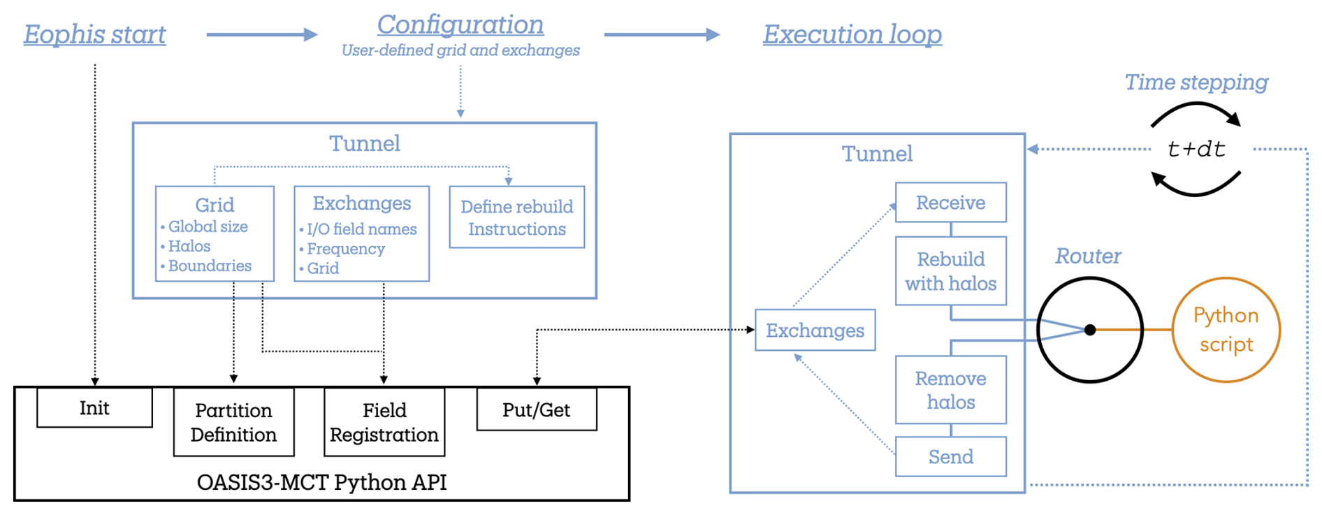
Figure 2 Eophis elements diagram. The Tunnel component is an OASIS3-MCT wrapper that configures the Python coupling API from the exchanges defined at the Eophis abstraction level. The Router configures the connections between received fields and the inputs of the Python functions, as well as between function outputs and the fields to be sent back. During execution, Eophis emulates the time-stepping to synchronize exchanges as the Earth System Model progresses in time: the Tunnel receives fields from the ESM (not represented) through OASIS3-MCT. These fields are passed to the Router, which dispatches them to the appropriate Python functions and collects the returned outputs. Once the outputs are available, the time-stepping instructs the Tunnel to send the resulting fields back through OASIS3-MCT, and the cycle repeats.

This highlights the need for a higher-level abstraction layer on the Python side that simultaneously (i) provides the missing features required by OASIS3-MCT usage, (ii) abstracts away the unnecessary coupling complexities, and (iii) enables flexible and automated configuration of the OASIS3-MCT Python API. We propose a Python library named Eophis, which encapsulates the OASIS3-MCT Python API within a generic Python coupling environment providing these functionalities. Any function from an external Python script can then be imported by the Eophis script to be used with the exchanged fields. Technically, Eophis is here the Python script coupled with the ESM³. This library also aims to generalize the configuration of OASIS3-MCT on the Python side through a simplified interface, and to provide tools to assist in setting up the global coupling environment, including the coupler namelist and ancillary files. Thus, it allows the user to flexibly define the data exchanges to perform. Figure 1 illustrates how Eophis operates as a Python script coupled with the Fortran ESM, bridging the Python script used for hybrid modelling with the OASIS3-MCT Python interface. It should be noted that each entity and the OASIS3-MCT communications may all be executed on CPUs. However, as discussed in Arnold et al. (2024), MPI-based communications of the coupling library make it possible to run the ESM and Python scripts as separate jobs. In this context, inserting GPU offloading instructions within the coupled Python script enables hybrid CPU/GPU modelling without modifications of the ESM.

3 Abstracting the deployment of ML models with Eophis

3.1 Scope and components of Eophis library

Eophis enables the coupling of Python scripts as standalone functions, abstracting away technical coupling challenges such as exchange execution, time synchronization, namelist configuration, and parallel communication. In this context, Python scripts are easily shareable and interchangeable. The resulting workflow for coupling an ESM with a Python script with Eophis can be described as follows: during execution, the ESM advances its time-stepping and sends fields to Eophis through OASIS3-MCT. Eophis receives these fields, routes them to the appropriate ML functions, collects the returned outputs, and sends the resulting fields back to the model through OASIS3-MCT before it resumes its computation. The execution cycle is repeated throughout the simulation in synchronization with the ESM time integration.

From the user’s perspective, this workflow reduces to the following description: “I want the ESM to send these fields, on this grid, to the Python function, receive the returned results, and repeat this process at a specified frequency”. Eophis is designed to encapsulate all the technical steps required on the Python side through APIs that directly reflect this user-level description. Three main elements structure this abstraction and are illustrated in Fig. 2: the Tunnel configures and performs the reception and sending of fields at the beginning and end of each cycle. The Router defines how received and returned fields map to the inputs and outputs of the Python-based ML components. The Time-stepping mechanism synchronizes the Python operations of the workflow with the temporal progression of the ESM. We describe in detail what these entities do in practice and how they give form to the generic Python coupling environment introduced in the previous section.

An exchange is the complete process that makes a field to be transferred from one coupled component to the other, including fields registration and call to the sending (put) and receiving (get) OASIS3-MCT functions during execution. The Tunnel reduces these steps on the Python side to the names of fields to receive and to send back (with the convention taken from the Python point of view). However, it is worth keeping in mind that each component is, in practice, parallelized and executed on its own dedicated pool of MPI processes. Thus, the sent and received fields are scattered among these processes, and OASIS3-MCT needs to know the local grid sizes expressed with global indexes to perform optimized partition-to-partition communications (see Fig. 3). If global sizes are different, OASIS3-MCT can also perform interpolation from one grid to another. However, the Eophis framework considers that identical grids are used on both sides. Describing the local partition for each Python process is still required in this configuration to set up communications. The Tunnel automates this partition description from the global 2D longitude and latitude dimensions.

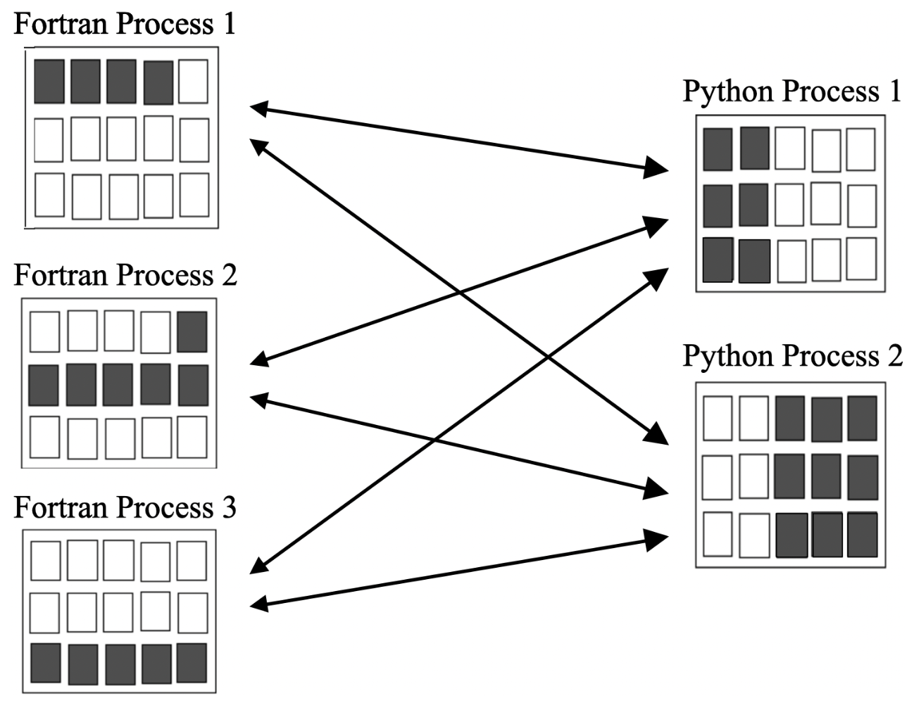
Figure 3 Multiple processes coupling principle diagram (without interpolation). Two exclusive pools of processes are allocated, respectively, with three processes for the Fortran Earth System Model and two for the Python script. The fields are scattered among processes on each side. OASIS3-MCT handles the communications between the pools and the redistribution to exchange the field from the processes of one model to those of the other.

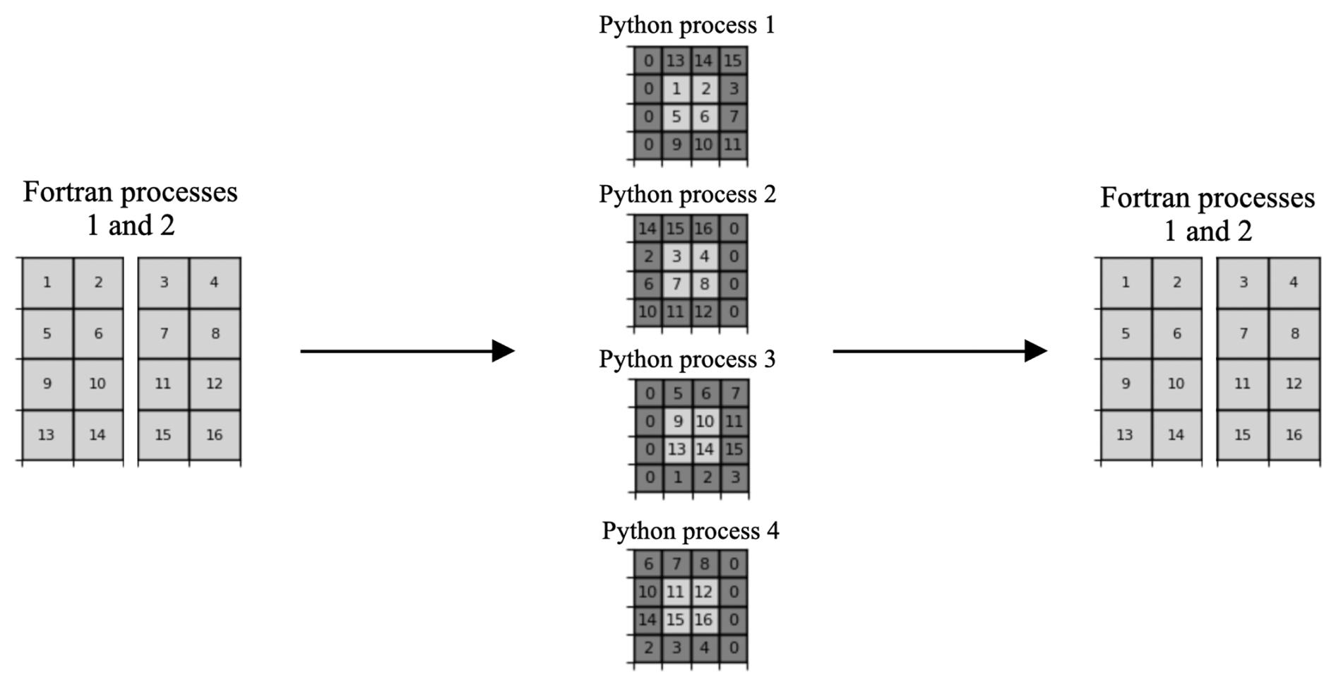
Figure 4 Halo reconstruction principle diagram. In regular coupling, each cell (in light gray) is communicated once between processes, as in Fig. 3. Eophis can configure OASIS3-MCT parallel features to communicate grid cells several times. The local grid from one Python process can receive a copy of cells (in dark gray) addressed to another Python process. They correspond to the neighboring cells of the local grid. Halo cells are present on the Python side to let the Python scripts work with array-like objects without the need for internal communications. These are ignored when sending back the coupling information from Python to Fortran processes. The number of halos and how to fill them at the boundaries are user parameters.

For some operations, such as differential calculus or use of Convolutional Neural Networks (CNN), it is necessary to know the neighboring cells of the local grid being processed. When local grids are located at the edges of the global grid, boundary conditions must be specified. These are required, in general, even in single-process simulations, as, for instance, in global model domains requiring periodic conditions. As illustrated in Fig. 4, grid cells can be divided into two parts: cells strictly contained in the local grid (real cells in light gray) and extra cells outside the local grid containing neighboring values (halos in dark gray). In classic OASIS3-MCT coupling, communications only involve real cells, as coupled ESMs have their own internal communication system to construct halos. In Eophis, halo reconstruction relies on two distinct steps. During the configuration phase, a specific OASIS3-MCT partition definition is used so that the communications include the additional cells required for halo construction. Then, during execution, Eophis performs intermediate reconstruction operations to rebuild the exchanged fields into grid-aware Python arrays with halo cells placed at their appropriate locations. Boundary conditions can also be specified to define values of halo cells that cross the global grid edges. This spares the need to create an internal communication system in the Python script, which has the twofold advantage of combining halo construction with field exchanges. Halos are automatically ignored when sending back a field. The particular OASIS3-MCT configuration for extended communications and the reconstruction procedure are also fully encapsulated within the Tunnel abstraction. At the user level, this is reduced to specifying the halo width and the boundary-condition treatment at global grid edges.

Once exchanges and grids have been defined, the Tunnel can call the OASIS3-MCT Python API to send and receive fields. The Router associates the names of the incoming fields defined within the Tunnel with the desired Python script inputs, and the Python function outputs with the names of the outgoing fields. Since coupling a different Python script implies different function signatures, this mapping must be adapted from one use case to another. Eophis therefore provides a flexible interface for configuring the Router connections.

The Time-stepping mechanism is the runtime abstraction responsible for orchestrating exchange calls according to the coupling configuration defined through the Tunnel and the Router. Since OASIS3-MCT requires both coupled components to expose a consistent temporal progression, Eophis mirrors the time advancement of the coupled ESM on the Python side. This hidden execution loop ensures that exchanges and Python function calls occur at the appropriate coupling times throughout the simulation.

Extra useful tools are also available with the Eophis library to automatically write the OASIS3-MCT namelist namcouple in accordance with defined exchanges and to read or write Fortran namelists. The latter helps to automate the Eophis execution, mirroring temporal and grid parameters, or transferring Eophis information into a Fortran-accessible object, for instance.

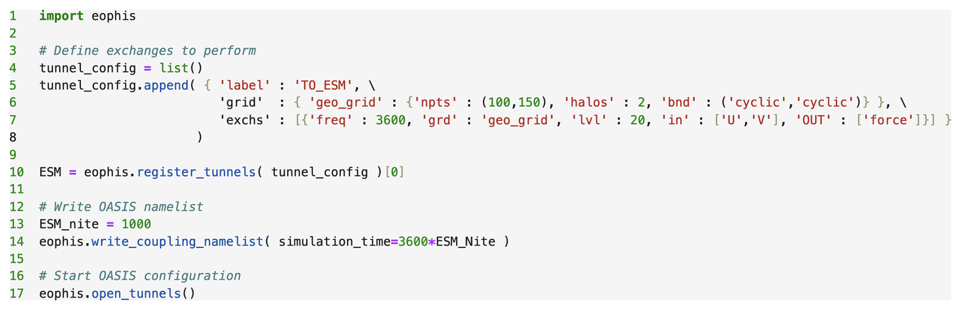
Figure 5 User-written Eophis code to define a Tunnel object. The latter gathers information on the global grid on which the fields are discretized, as well as exchanges to perform. The Tunnel is registered in Eophis' memory to prepare the OASIS3-MCT namelist and configuration.

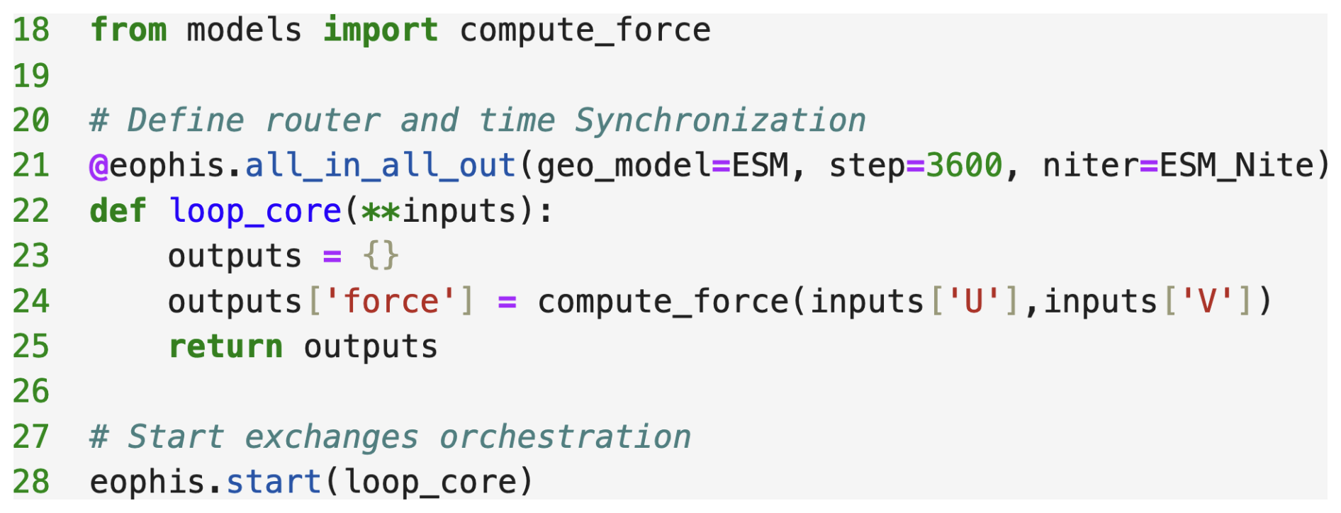
Figure 6 User-written Eophis code to define time synchronization of exchanges and the connections between exchanged fields.

3.2 Eophis interface

We give here minimal examples of how Eophis can be used in practice. As mentioned in the previous section, the Eophis API reduces all coupling operations to what the user wants to exchange and link. Let us suppose that we wish an ESM to send two fields, named U,V, every hour to a Python script that returns a single forcing term named force. We know that the fields are discretized on the 20 levels of a periodic grid of size (100,150). Additionally, the Python script is a CNN whose receptive field is a 5 × 5 square, meaning that two halos are required at the edges of the local grid. We write the Eophis script from this information to couple the CNN with the ESM through OASIS3-MCT. First, the exchanges should be summarized in the abstraction class Tunnel, whose definition is shown in Fig. 5. We define a grid (code line 6) from the global number of longitude and latitude points. The number of wished halos and boundary conditions is also specified. Line 7 of the code is a list of parameters that describe how the fields should be exchanged. It can be read as: every 3600 s, receive the fields U,V and send back the field force on the first 20 levels of grid geo_grid. It is also possible to define several exchanges in the same Tunnel, with only incoming or outgoing fields, or different frequencies or grids, for instance. The functions write_coupling_namelist() and open_tunnels() generate the OASIS3-MCT namelist namcouple and configure the OASIS3-MCT Python API, respectively, from the Tunnel's attributes. The corresponding namcouple for this example is available in Appendix A.

The next step is to set up the Python time synchronization and connections between the received fields and the fields to send back. Here, force is the result of the Python script with U,V passed as arguments. The Eophis interface for these components is shown in Fig. 6. First, the function compute_force() is imported, as it is the Python operation external to Eophis. The all_in_all_out() decorator defines the time orchestration of exchanges. It takes a Tunnel to work with, the number of temporal iterations, and the time step value. The definition of connections between received and sent back fields is done within the loop_core() function. All the Tunnel's received fields (i.e., those identified as in in Tunnel) are present in the inputs dictionary. The user defines here to which imported functions they should be sent, and how to fill the content of outputs, whose keys correspond to the fields to send back (identified as out in Tunnel). It should be noted here that all these components describe pipelines only. The choice of the values contained in the arrays to pass through OASIS3-MCT and the specific operations to perform should be done by the Python model and the ESM.

From now on, OASIS3-MCT needs to be configured in the ESM in accordance with the coupling context defined through Eophis. Although this part strongly depends on how OASIS3-MCT has been implemented in the ESM, useful information can be found in the Eophis logs to help in this part of the configuration (see Appendix A). The agreement between coupled and standalone Python script calculations and the correctness of halo reconstruction across MPI partitions were checked by running the non-regression tests and tutorials provided with Eophis sources⁴.

4 Computational performance of hybrid modelling with Eophis

4.1 Benchmark cases

We evaluate wall-clock performance and resource allocation for hybrid modelling with OASIS3-MCT and Eophis with the ocean general circulation model NEMO version 4.2.1, coupled with different Python scripts. Given that NEMO and the Python scripts are executed independently, the first benefit of using couplers is the flexibility in setting the number of MPI processes for each component. We highlight this feature by setting up two test cases using a $\mathrm{1}/\mathrm{4}$° global ocean NEMO configuration with 75 depth levels (eORCA025.L75).

In the first test case, NEMO is coupled with a Python script containing the ML-based Mixed Layer Eddies closure proposed by Bodner et al. (2025). The latter leverages data-driven methods to take into account the complex relationships between mixed layer vertical buoyancy fluxes and the large-scale physics observed in recent studies (Bodner et al., 2023; Zhang et al., 2023b). The approach relies on a CNN trained to infer vertical buoyancy fluxes $\stackrel{\mathrm{‾}}{w^{\prime }{b}^{\prime }}$ from the large-scale buoyancy gradient, Coriolis parameter, mixed layer depth, air–sea fluxes, horizontal divergence, vertical vorticity, and strain. All fields are 2D, vertically averaged over the mixed layer depth to remain consistent with the original Fox-Kemper et al. (2011) formulation. Building on this, the returned vertical buoyancy flux is used to compute the velocity streamfunction Ψ representing the unresolved eddy effects by inverting $\stackrel{\mathrm{‾}}{w^{\prime }{b}^{\prime }}=\mathbf{\Psi }\times {\mathbf{\nabla }}_H{\stackrel{\mathrm{‾}}{b}}^z$, where the last term is the horizontal buoyancy gradient. The streamfunction is finally applied over depth using the vertical structure function proposed by Fox-Kemper et al. (2011) to update the NEMO velocity transport. All operations on 3D fields are performed by NEMO, and only the 2D fields required for inference are exchanged. This case is hereafter referred to as 2D.

In the second test case, NEMO is coupled with a Python script containing the deterministic density correction ${\mathit{\rho }}_{\mathrm{c}}=\frac{{\partial }^{\mathrm{2}}\widehat{\mathit{\rho }}(T,S)}{\partial T^{\mathrm{2}}}c\mathrm{|}\mathit{\delta }\circ \mathbf{\nabla }\stackrel{\mathrm{‾}}{T}{\mathrm{|}}^{\mathrm{2}}$ proposed by Stanley et al. (2020) to correct for small-scale fluctuations of temperature and salinity. Here, c is a constant, $\mathit{\delta }=({\mathit{\delta }}_x,{\mathit{\delta }}_y)$ is the grid-scale length vector, ∘ is the Hadamard product, and $\widehat{\mathit{\rho }}(T,S)$ is the density calculated by the equation of state from temperature and salinity. The script leverages the Python API of the Gibbs SeaWater oceanographic toolbox TEOS-10 (McDougall and Barker, 2011) to compute the second derivative of the equation of state. The density correction is then returned to update the NEMO density field. All 75 grid levels of the temperature, salinity, and density correction are exchanged here. The case is hereafter referred to as 3D.

A first set of 2D and 3D cases is executed with both NEMO and the Python script running on CPU cores. The number of MPI processes allocated to NEMO is kept fixed, while the number of MPI processes for the Python script varies. Each MPI process is mapped to one CPU core. The 2D cases are run twice. In the second run, the Python script is still executed on CPU cores but the inference is offloaded to GPUs (1 for every 40 CPU cores allocated to the Python script) ⁵.

Each test case is first executed with a synchronous implementation, that is, NEMO sends the inputs, and then waits for the Python script results, as would be the case for any in-built NEMO function. Cases in this configuration are denoted hereafter with the -S suffix (2D-S for instance). Taking advantage of the parallel-execution capabilities offered by the couplers, we then reproduced each test case by changing the coupling implementation from synchronous to asynchronous. In the latter, NEMO sends the inputs as soon as possible in the time loop, and continues computation as far as possible, i.e., until it needs the fields processed by the Python script. Importantly, although the coupling is asynchronous in terms of execution, it remains synchronous in terms of model time. The input and output fields exchanged within a coupling step correspond to one same NEMO time step, and no temporal lag is introduced. The cases in this configuration are denoted hereafter with the -A suffix.

Each simulation consists of 1000 time steps, executed in two separate chunks. They were carried out on a HPE SGI 8600 supercomputer at the French CNRS computing center IDRIS JeanZay. The supercomputer consists of 720 nodes, each equipped with 40 Intel Xeon Gold CPU cores and 4 NVIDIA GPUs Tesla V100 SXM2 16Go. The nodes are connected to an Intel Omni-Path 100 series and use a Lustre file system. For all simulations, the allocated computing nodes are used exclusively. The software environment is based on a Linux RedHat 9.6 operating system and the Slurm 23.11.3 workload manager. Parallel computations rely on OpenMPI 4.1.5, while the numerical codes are compiled using GCC 10.1.0 and CUDA 11.2 for GPU computations. The Python scripts were executed using Python 3.11.7 and PyTorch 2.2.0. NEMO was compiled with NetCDF-C 4.7.4 and NetCDF-Fortran 4.5.3, together with HDF5 1.12.0.

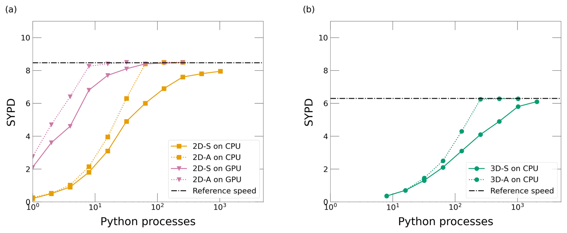
Figure 7 (a): NEMO simulation speed in Simulated Year Per Day for eORCA025.L75 as function of the number of MPI processes allocated to the 2D case Python script with inference executed on CPUs and on GPUs, and for different coupling implementations, asynchronous (-A) and synchronous (-S). The number of MPI processes allocated to NEMO is fixed and equal to 999. (b):(b)Same with the 3D case Python script executed on CPUs.

4.2 Scalability

We first discuss the results for the test cases executed with the synchronous implementation. The asynchronous cases are treated in the next section. Figure 7 shows the number of Simulated Year Per Day (SYPD) for the simulations for (a) the 2D case with inference executed on CPUs and on GPUs, and (b) the 3D case executed on CPUs only (continuous curves for synchronous implementation). The SYPD values are computed from the average wall-clock time per time step over all time steps of a given simulation. The number of MPI processes allocated to the Python script is increased by successive doublings and follows integer powers of two. The performance for the eORCA025.L75 configuration without coupling is also shown as a reference speed to be reached⁶. Unsurprisingly, it is seen that the addition of the coupling context causes the simulation speed to fall for all cases. Fortunately, this loss can be easily balanced by allocating more processes to the Python script. For the 2D case executed on CPUs only (curves with squares), allocating additional processes of roughly 30 % of those assigned to NEMO (a bit more than 256 extra Python processes over 999 NEMO processes) brings the simulation speed close to the reference performance, although it remains clearly lower. Beyond this point, increasing allocation up to an order of magnitude similar to NEMO yields little improvement, indicating a plateau in performance gains. A more detailed analysis of the shape and behavior of the SYPD curves is provided in Appendix B. The time overhead incurred by running the inference on the CPUs allocated to the Python script can be overcome by offloading the inference on GPUs (curves with triangles). The order of magnitude of the additional MPI process requirement to match the reference in this case can be located around 6 % of those allocated to NEMO (64/999), corresponding to 64 CPU cores, in addition to two GPUs for the inference. For the 3D case, achieving performance close to the reference requires more than 2048 additional Python processes, corresponding to more than 200 % of the NEMO processes, although the reference performance is still not fully reached.

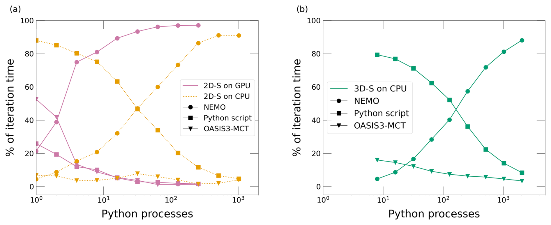
Figure 8 (a) Averaged percentage of time distribution of a NEMO iteration between OASIS3-MCT routines, execution of the 2D case Python script and NEMO routines with the synchronous (-S) implementation for eORCA025.L75 as a function of the number of MPI processes allocated to the 2D case Python script. (b) Same with the 3D case Python script executed on CPUs.

Table 1 Root-Mean-Square Error (RMSE) of the heat flux correction predicted by the Storto et al. (2025) ML model and of the raw output of the NN between different implementations: Fortran (ORCA1-F), Infero (ORCA1-I), Eophis (ORCA1-E), and Fortran compiled using the ORCA1-E build (ORCA1-F^∗). The RMSE of the NN output is normalized by its standard deviation.

Figure 8 provides more insight into the origin of the time-to-solution overhead. It shows the average percentage of time spent per NEMO iteration by different steps in the synchronous implementation. Despite the 3D case involving more OASIS3-MCT operations due to the size of the grid, the percentage of time spent on OASIS3-MCT routines remains comparable across all test cases. It decreases as the number of processes allocated to Python increases, but not significantly. However, changing the number of Python processes has a clear impact on the time spent on Python operations. As can be expected, a notable difference in the computation time between the Python scripts of the 2D and 3D cases can be observed for a given number of processes. As the Python scripts for the 2D and 3D cases differ in terms of computational needs, the separation of the resource allocation appears here as a suitable strategy for exploring different Python hybridization approaches while accounting for the specific computational characteristics of each case. This observation also provides some perspective on the choice of hardware for the Python script. Discussing the cost/benefit trade-offs of using GPUs vs CPUs for neural network inference lies outside the scope of this study. Nonetheless, we stress that small neural networks can generally run efficiently on CPUs, while GPUs are adapted to running deep neural networks due to their parallel processing capabilities (Gyawali, 2023). The cost/benefit trade-offs of using GPUs also depend on several other factors, in particular the evolution of the price and availability of GPUs for scientific computing because of the high demand on GPUs at global scale (Durand et al., 2026).

4.3 Asynchronous coupling

The synchronous implementation is obviously suboptimal since reducing NEMO waiting time implies allocating more and more computational resources to the Python script to make its execution faster. We now compare the SYPD between synchronous and asynchronous implementations in Fig. 7. We can observe that the additional number of Python processes required to maintain the reference time-to-solution is generally smaller in the asynchronous strategy compared to the corresponding synchronous cases. It decreases to less than 1 % of the processes allocated to NEMO for the 2D case with inference executed on GPUs (8 additional Python processes over 999 NEMO processes, in addition to a single GPU for the inference). More notable is the extra process requirement for the 2D case with inference on CPUs that falls around 6 % (64/999). Similarly, the additional processes in the 3D case are reduced to an order of magnitude of 25 % (256/999). Every asynchronous test case exhibits a plateau immediately after a discontinuity. It corresponds to the moment from which NEMO no longer waits for the Python scripts. Allocating more computational resources to the Python script after this point is useless. The interpretation of the SYPD curve behavior for this kind of implementation can be found in Appendix B. As an additional consistency check, we compared the results obtained with the synchronous and asynchronous implementations by computing the root-mean-square error (RMSE) between the time-averaged fields over one simulated day of the density correction returned by the Python script for the 3D-S and 3D-A cases. The normalized RMSE was 0.4 %, indicating close agreement between the two implementations. This comparison was not performed for the 2D cases.

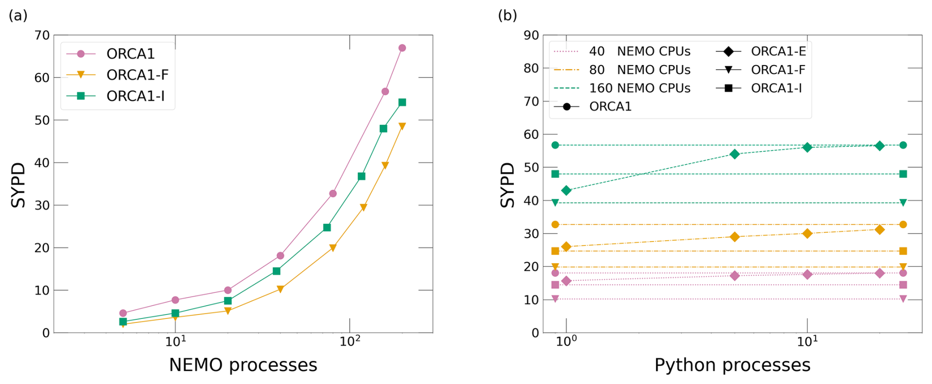
Figure 9 (a) Simulation speed in Simulated Year Per Day as a function of the number of MPI processes allocated to NEMO for different implementations of the Storto et al. (2025) ML model: NEMO without ML model (ORCA1), with Fortran (ORCA1-F), and Infero (ORCA1-I). (b) Simulation speed in Simulated Year Per Day for ORCA1-E as a function of the number of MPI processes allocated to the Python script for different number of processes allocated to NEMO. Results are compared for different implementations of the Storto et al. (2025) ML model: NEMO without ML model (ORCA1), with Fortran (ORCA1-F) and Infero (ORCA1-I). Lines for those cases are here for readability as their values are fixed and independent of the number of Python processes.

4.4 Comparison with other solutions

For completeness of the evaluation, we compared the computational performance of OASIS3-MCT and Eophis with other hybrid modelling methods. The benchmarking is based on the case of Storto et al. (2025) (S24 hereafter) in which a ML model is used to correct the air–sea heat fluxes in the NEMO 1° global ocean circulation configuration (ORCA1). Here, version 4.0.7 of the NEMO model is used, according to S24. In the S24 study, the ML model is an in-house Fortran-written NN whose weights have been saved in NetCDF format. In a first step, we duplicated the NN and the weights with the Keras library in TensorFlow-readable format. Then, we performed three realizations of the simulation described in the paper with different implementations of the NN. The first is the exact reproduction of the original study (ORCA1-F), while the second implements the Infero (Bonannim and Quintino, 2024) Fortran API, version 2.0 with TensorFlow 2.6.0, in NEMO to load the TensorFlow version of the NN and use it for inference (ORCA1-I). In the third case, instructions for loading and using the TensorFlow version of the NN for inference are encapsulated in a Python function. The latter takes the inputs required by the NN as arguments. The Python script containing this function is coupled to NEMO through OASIS3-MCT with the help of Eophis (ORCA1-E). For ORCA1-E, the inference is computed with TensorFlow 2.11.0 on CPUs, and the coupling implementation is synchronous, similarly to the sequential implementation of the NN for ORCA1-F and ORCA1-I. A final test case in which the ML model is not used is also performed as a reference, hereafter denoted as ORCA1. We first ensured that converting the original Fortran NN into different formats did not modify its predictive performance. We performed a five-day simulation of the ORCA1-F, ORCA1-I and ORCA1-E cases and extracted the time-averaged fields of the output of the NN and the resulting surface heat flux correction. For each field, we quantified the differences between the three cases by computing the RMSE between each pair of fields. The results are presented in Table 1. It is seen that the fields computed with OASIS3-MCT and Eophis differ slightly from the fields computed in ORCA1-F and ORCA1-I. Our investigation revealed that this difference is mostly located along the coastlines and originates from a discrepancy between NEMO builds compiled with and without OASIS3-MCT. As a confirmation, we have verified that the observed RMSE differences are reduced to the order of magnitude of those between ORCA1-F and ORCA1-I when NEMO is compiled from sources that include OASIS3-MCT (ORCA1-F*). Since the scope of this study is to assess the performance of the different NN implementations, investigating the origin of this discrepancy within the NEMO code, as well as quantifying its impact on the physical relevance of the results, is beyond the scope of this paper. Nevertheless, the application of OASIS3-MCT and Eophis to another study revealed a similar behavior, which appeared to be related to runoff fields. This observation provides a potential direction for future investigations.

We now focus on the wall-clock performance of the different implementations of the NN. A comparison of the SYPD between ORCA1, ORCA1-F, and ORCA1-I against the number of processes allocated to NEMO is shown in Fig. 9a. The values are computed with the averaging procedure described in Sect. 4.4. As expected, ORCA1 runs the fastest since the NN is not activated. ORCA1-I and ORCA1-F show a slight decrease in speed compared to ORCA1, with ORCA1-F being slower than ORCA1-I. However, overall performance and scalability remain comparable across configurations. To compare the performance between these cases and ORCA1-E, we fixed the number of processes assigned to NEMO to three different values (40, 80 and 160). We then varied the number of processes allocated to the Python script. The resulting curve is compared with the ORCA1, ORCA1-F, and ORCA1-I SYPD values corresponding to the fixed number of NEMO processes, as shown in Fig. 9b. We can observe that the performance of the Eophis implementation (ORCA1-E) for a low number of Python processes is comparable to that of Infero. As also illustrated previously, increasing the number of Python processes makes the inference computation faster. For all the chosen numbers of NEMO processes, it is possible, for ORCA1-E, to recover the simulation speed of the reference case (i.e., NEMO without ML model) at a high number of Python processes. It should be noted that the size of the inputs in the S24 configuration is quite light. An interesting supplementary study to this benchmark would be to evaluate how the different implementation methods scale with the input size or the number of computational operations required by the inference.

5 Discussion

5.1 Limitations

In our effort to use and evaluate OASIS3-MCT with Eophis, we remained limited to applications of hybrid modelling that involve inference only. Although it is possible in practice to couple an ESM that would only send inputs to a Python script to train a neural network, we do not think that it would be the most adapted tool for this kind of application. The important data stream required for training could be a limiting factor, given the architecture of OASIS3-MCT. Alternative coupling libraries with more advanced data-handling capabilities may therefore provide a more suitable basis for online training. Recent developments in projects such as Melissa (Schouler et al., 2023) or XIOS point in this direction. However, evaluating the performance of OASIS3-MCT for training neural networks with relatively light architectures, or those that do not require inputs at every time step, or only partial re-training, would be of interest.

Practical deployment aspects must also be considered. Despite all the aforementioned advantages of using coupling libraries for hybrid modelling, the additional software layer required to deploy a coupled configuration can be harsh, depending on the user's expertise in coupling tools. A typical situation where this approach might become suboptimal is for an ML parameterization implemented in an operational ESM. Here, since the use of the ML components is expected to be regular, a permanent implementation using Fortran ML library APIs may be easier to run and maintain than relying on coupling libraries. Nevertheless, similar to the study by Zhang et al. (2023a), this kind of uncoupled implementation might require additional MPI communications within the Fortran code itself. Indeed, depending on the architecture of the neural network, users may need to reconstruct halos or redistribute fields in a more optimized grid decomposition, which can be a challenge in terms of development effort. Hence, thanks to the interchangeability of Python scripts, coupler-based methods appear advantageous for prototyping and quick testing of new parameterizations before addressing the question of permanent integration.

5.2 Future perspectives

We emphasize here that Eophis is a utility software that does not perform the coupling itself but leverages the Python API of OASIS3-MCT. This backend could be extended to support other coupling libraries offering such an API, without requiring changes to the Eophis abstraction layer. At the time of writing, and to our knowledge, most coupling libraries used in ESMs do not yet provide Python support, except YAC (Hanke and Redler, 2019) and XIOS, or are still under development, making OASIS3-MCT central to this work. In any case, most of these libraries rely on design assumptions similar to those of OASIS3-MCT, namely symmetric ESM features between coupled components. While Eophis is a proposal for facilitating the use of current ESMs coupling tools for hybrid modelling, we hope this work to serve as feedback for the next generation of couplers, which should explicitly account for the asymmetry for coupling ESMs with Python routines.

In the long term, the need for bridging strategies (see Sect. 2.1) may be transitional. As noted in Sect. 2.1, several ESM components are now being implemented in high-level languages, sometimes with the assistance of AI coding agents. Entire ESMs may soon be coded in JAX, Julia, or PyTorch. In such systems, bridging strategies across languages would no longer be required, as neural networks could be natively integrated within the same runtime environment. The authors consider this prospect capable of enabling the radical transition or paradigm shift anticipated by Shaw and Stevens (2025), allowing scientists to more easily deploy hierarchies of ESMs of varying complexity.

5.3 Sharing experiments

Being a promising new field, hybrid modelling naturally raised many concerns, both in terms of scientific relevance and practical application. In this conclusion, we wish to address the latter. While intense efforts have been made to investigate ways of calling ML from Fortran, several practical aspects remain underexplored. As mentioned earlier, integrating ML components into ESMs requires additional complex software layers. This raises the question of how to account for such obstacles in the broader goal of making hybrid modelling experiments easily reproducible. Ensuring that the weights and biases of ML models are preserved and accessible is also crucial in this regard. Therefore, we need to explore new ways to evolve and strengthen best practices for reproducible hybrid modelling. Moreover, the wide variety and complexity of existing solutions for deploying ML components in physics-based models currently make the establishment of standard procedures for sharing code and experiments highly challenging. As a step toward addressing this issue, we present the solution we have adopted to share the ocean hybrid modelling experiments we performed with the help of Eophis in the Appendix C. All test cases conducted in this study are stored following this solution and are openly available (see “Code and data availability” section). We do not claim to provide a definitive solution for the sharing of reproducible hybrid experiments. Rather, this work should be regarded as a proposed contribution, which may help inform and inspire future practices.

6 Summary

In this paper, we have explored how coupling libraries present in Earth System Models can be used for implementing code components written in Python, as for instance, pre-trained Machine Learning (ML) components. This approach allows two codes to be executed simultaneously and independently; the former is an ESM, while the latter is a Python script that contains instructions to use the ML component for inference. Both exchange data through the coupling interface as the simulation progresses. Many benefits of this method have been identified. Since ESMs are written in Fortran and ML components in Python, the first possibility is to split up the simulation into two heterogeneous programming environments. The Fortran-Python bindings development work is limited here to the coupler interface. Thus, the operations required to compute and pass the geophysical fields to the ML component are performed in the ESMs, where the numerical tools are the most adapted; operations related to the manipulation of the ML component inputs and outputs are then isolated within the coupled Python script. Similarly, the appropriate integration of the fields returned by the ML component in the simulation is done within the ESM, according to the solver algorithms. Our experience demonstrated that this feature eases the collaboration between climate modelers and computer scientists, with each community being able to work in their preferred environment. Separation into two independent codes also unlocks parallel work. In this context, computing resources can be distributed flexibly and asymmetrically between components, allowing both to work with a differently optimized decomposition. Moreover, the reconstruction of the global geophysical fields is operated through the MPI routines of the coupling library, which is essential for performance. Finally, the low intrusiveness of this method makes the Python scripts containing the ML components easily shareable between different physics-based models, may they include an implementation of the coupling library. In this work, the OASIS3-MCT coupling library has been chosen to couple Python scripts containing ML components with ESMs because it already possesses Fortran and Python APIs, in addition to being widely present in the climate modelling codes.

However, we also highlighted that although coupler-based frameworks enable hybrid Fortran-Python coupling, their design targets ESM-ESM interactions and is therefore not well suited to ESM-ML applications. ML components indeed act as passive functions driven by the ESM and lack several features commonly implemented in ESMs and expected by coupling libraries, leading to additional unnecessary complexity in the Python scripts.

To address this, we introduced Eophis, a generic OASIS3-MCT coupled Python component that provides the required features to bridge any function imported from an external Python script with an ESM coupling interface, including useful functionalities such as exchange execution, time synchronization, reading and writing of namelists, parallel communication, and guidance for configuring the coupling layer on the ESM side. The Eophis interface eases the configuration of the coupling API on the Python side by abstracting the definition of the exchanges to perform between the ESM and the Python script. It also allows the user to define, if necessary, the mapping between the received data and the data to send back. This design enables the Python coupling environment to be easily adapted to the requirements of the imported Python functions, keeping them coupling-independent and readily interchangeable.

The wall-clock performance and resource allocation of hybrid ESM-ML modelling with OASIS3-MCT and Eophis have been evaluated by coupling 2D and 3D Python ML and analytical scripts with the ocean general circulation model NEMO, chosen arbitrarily among the OASIS3-MCT-equipped ESMs compatible with this framework. Experiments have illustrated that running NEMO and the Python script as separate jobs allows computational resources to be optimally allocated to each component. The proposed solution allows in particular to leverage GPUs for accelerating the execution of the Python script while using CPUs for running NEMO. A key feature of the proposed solution is the possibility to run the computation threads in parallel. This asynchronous coupling enables to minimize the waiting time of the ESM, so that in practice the impact of running the Python script on the overall time-to-solution is almost negligible, provided sufficient computing resources are allocated to the Python script. Compared to a sequential coupling of the Python script, the additional resources required to reach a given simulation speed under asynchronous conditions has been divided by eight to 18 for the test cases considered in this study. Finally, we have compared the execution speed of hybrid models run with OASIS3-MCT with deployment based on two existing wrappers of ML libraries. Our results show that, for the ORCA1 benchmarks considered in this study, hybrid models deployed with OASIS3-MCT achieve the shortest time-to-solution, provided enough resources are allocated to the execution of the Python scripts.

Appendix A: Additional details about files generated by Eophis

Figure A1a shows an example of the Eophis log for writing the OASIS3-MCT namelist namcouple, according to the example given in Sect. 3.2. The latter is filled with information about the Eophis version, dependencies, and Python implementation. We can also note the Coupling Initialization part. When Eophis starts, it automatically looks for the OASIS3-MCT coupling namelist to read its content. If namcouple exists, it is read and copied as namcouple_ref. If namcouple does not exist but namcouple_ref does, the reference namelist is copied, then read. If both files exist, namcouple is read. Finally, if none of the files exist, Eophis creates an empty namcouple. This behavior allows for the scenario where the user wishes to couple a Python script with a first ESM that is also coupled with another ESM. Since only one coupling namelist is required by OASIS3-MCT to perform all the exchanges, the user may bring their own namcouple with pre-written information about the coupling between the ESMs, and use Eophis to complete it with the Python coupling information. For a user who does not know about namcouple or does not wish to write it, the default case makes its creation straightforward.

We now emphasize the content of the OASIS3-MCT namelist generated by Eophis in Fig. A1b. Regular OASIS3-MCT users may notice that the first two terms for a given namcouple section do not match names defined in the Tunnel. Those are indeed aliases that OASIS3-MCT uses to perform the communications. OASIS3-MCT manipulates U under the name E_OUT_0 on the ESM side, and under M_IN_0 on the Python side. Those aliases have been set by default during Tunnel registration. In Eophis, it does not matter to know these aliases, since all OASIS3-MCT actions are wrapped. On the contrary, it might matter in the geoscientific code to configure the coupling. To help setting up the coupling from the ESM side, the mapping between Tunnel field names and OASIS3-MCT aliases can be found in the Eophis log (see Fig. A1a). Another solution is to make the ESM read the eophis_nml file generated by Eophis. This file contains the aforementioned mappings in Fortran namelist format. It is intended to help adapt the call of the OASIS3-MCT API on the Fortran side, according to the Tunnel definition. This approach requires the development, at least once, of a Fortran module responsible for carrying out this procedure, according to how the OASIS3-MCT API has been implemented in the ESM. Such a module has been used with NEMO for the test cases conducted in this study. It can be found and serves as template within our sharing platform presented in Appendix B.

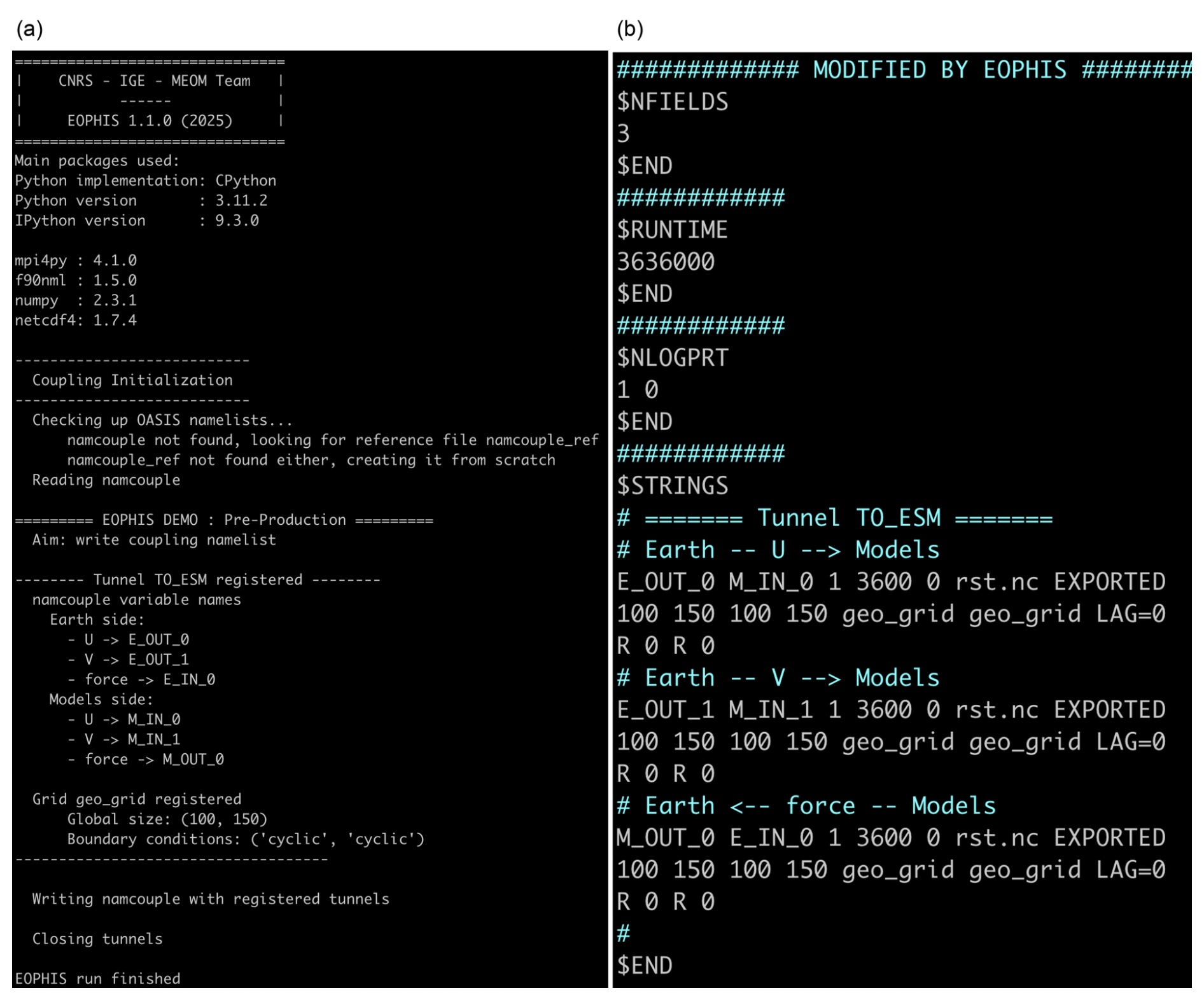
Figure A1 (a): Eophis log for writing namcouple. (b): Content of the OASIS3-MCT namelist namcouple generated by Eophis.

Appendix B: Runtime and scalability analysis

We analyze the behavior of the curves presented in Fig. 7 to identify scaling trends for estimating simulation speed from simple variables. We suppose the execution time of the Fortran Earth System Model (ESM) is τ_f and the Python script is τ_p. The time cost needed to advance the whole system for one time step with the synchronous implementation is

$$\begin{array}{}\text{(B1)}& {\mathit{\tau }}_{\mathrm{s}}={\mathit{\tau }}_{\mathrm{f}}+{\mathit{\tau }}_{\mathrm{p}},\end{array}$$

where the time taken by the OASIS3-MCT communications is assumed to be negligible.

Let us now recall that in the asynchronous implementation, the ESM sends the fields to the coupled Python script at the beginning of the time step. It then performs operations until the moment at which the Python results are required and optionally waits for Python results. Once received, it performs the last operations to finish the time step. In this situation, the execution time with the asynchronous implementation becomes

$$\begin{array}{}\text{(B2)}& {\mathit{\tau }}_{\mathrm{a}}={\mathit{\tau }}_{{\mathrm{f}}_{\mathrm{1}}}+{\mathit{\tau }}_{{\mathrm{f}}_{\mathrm{w}}}+{\mathit{\tau }}_{{\mathrm{f}}_{\mathrm{2}}},\end{array}$$

with ${\mathit{\tau }}_{{\mathrm{f}}_{\mathrm{1}}}$ the time for the Fortran code to execute the operations prior to those requiring the Python results, ${\mathit{\tau }}_{{\mathrm{f}}_{\mathrm{w}}}$ the waiting time for the Python results, and ${\mathit{\tau }}_{{\mathrm{f}}_{\mathrm{2}}}$ the time taken by the ESM to finish the time step after receiving the Python results. Also ${\mathit{\tau }}_{\mathrm{f}}={\mathit{\tau }}_{{\mathrm{f}}_{\mathrm{1}}}+{\mathit{\tau }}_{{\mathrm{f}}_{\mathrm{2}}}$ by definition.

If ${\mathit{\tau }}_{\mathrm{p}}<{\mathit{\tau }}_{{\mathrm{f}}_{\mathrm{1}}}$, then ${\mathit{\tau }}_{{\mathrm{f}}_{\mathrm{w}}}=\mathrm{0}$, otherwise ${\mathit{\tau }}_{{\mathrm{f}}_{\mathrm{w}}}={\mathit{\tau }}_{\mathrm{p}}-{\mathit{\tau }}_{{\mathrm{f}}_{\mathrm{1}}}$. The time cost for the asynchronous implementation is then

$$\begin{array}{}\text{(B3)}& {\mathit{\tau }}_{\mathrm{a}}={\mathit{\tau }}_{\mathrm{f}}-{\mathit{\tau }}_{{\mathrm{f}}_{\mathrm{1}}}+max({\mathit{\tau }}_{{\mathrm{f}}_{\mathrm{1}}},{\mathit{\tau }}_{\mathrm{p}}).\end{array}$$

The time cost of the Python models execution used in this study is perfectly scalable (not shown). Then

$$\begin{array}{}\text{(B4)}& {\mathit{\tau }}_{\mathrm{p}}={\displaystyle \frac{{\mathit{\tau }}_{\mathrm{p}}^{\ast }}{N_{\mathrm{p}}}},\end{array}$$

where N_p is the number of MPI processes allocated to the Python script, and ${\mathit{\tau }}_{\mathrm{p}}^{\ast }$ is the time cost when N_p=1. We can see

$$\begin{array}{}\text{(B5)}& {\displaystyle }& {\displaystyle }{\mathit{\tau }}_{\mathrm{s}}={\mathit{\tau }}_{\mathrm{f}}+{\displaystyle \frac{{\mathit{\tau }}_{\mathrm{p}}^{\ast }}{N_{\mathrm{p}}}}={\mathit{\tau }}_{\mathrm{f}}\left(\mathrm{1}+{\displaystyle \frac{{\mathit{\tau }}_{\mathrm{p}}^{\ast }}{{\mathit{\tau }}_{\mathrm{f}}}}{N}_{\mathrm{p}}^{-\mathrm{1}}\right),\text{(B6)}& {\displaystyle }& {\displaystyle }{\mathit{\tau }}_{\mathrm{a}}={\mathit{\tau }}_{\mathrm{f}}\left(\mathrm{1}-{\displaystyle \frac{{\mathit{\tau }}_{{\mathrm{f}}_{\mathrm{1}}}}{{\mathit{\tau }}_{\mathrm{f}}}}+max\left[{\displaystyle \frac{{\mathit{\tau }}_{{\mathrm{f}}_{\mathrm{1}}}}{{\mathit{\tau }}_{\mathrm{f}}}},{\displaystyle \frac{{\mathit{\tau }}_{\mathrm{p}}^{\ast }}{{\mathit{\tau }}_{\mathrm{f}}}}{N}_{\mathrm{p}}^{-\mathrm{1}}\right]\right).\end{array}$$

The simulated year per day (SYPD) is $\text{dt}/(\mathrm{365}\cdot \mathit{\tau })$, with dt the simulated time during one time step, and τ the time cost, either τ_s or τ_a. This leads to

$$\begin{array}{}\text{(B7)}& {\displaystyle }& {\displaystyle }{\text{SYPD}}_{\mathrm{s}}={\displaystyle \frac{\text{dt}}{\mathrm{365}\cdot {\mathit{\tau }}_{\mathrm{f}}}}{\left(\mathrm{1}+{\displaystyle \frac{{\mathit{\tau }}_{\mathrm{p}}^{\ast }}{{\mathit{\tau }}_{\mathrm{f}}}}{\mathrm{10}}^{-x}\right)}^{-\mathrm{1}},\text{(B8)}& {\displaystyle }& {\displaystyle }{\mathrm{\text{SYPD}}}_{\mathrm{a}}={\displaystyle \frac{\text{dt}}{\mathrm{365}\cdot {\mathit{\tau }}_{\mathrm{f}}}}{\left(\mathrm{1}-{\displaystyle \frac{{\mathit{\tau }}_{{\mathrm{f}}_{\mathrm{1}}}}{{\mathit{\tau }}_{\mathrm{f}}}}+max\left[{\displaystyle \frac{{\mathit{\tau }}_{{\mathrm{f}}_{\mathrm{1}}}}{{\mathit{\tau }}_{\mathrm{f}}}},{\displaystyle \frac{{\mathit{\tau }}_{\mathrm{p}}^{\ast }}{{\mathit{\tau }}_{\mathrm{f}}}}{\mathrm{10}}^{-x}\right]\right)}^{-\mathrm{1}}.\end{array}$$

Here, x is the log coordinate as shown in Fig. 7, such that 10^x=N_p. These expressions reproduce the main features of the curves shown in Fig. 7. For the synchronous implementation, the curve is S-shaped and approaches a maximum as x→∞.

For the asynchronous implementation, the behavior is initially exponential in 10^x, and SYPD_s≈SYPD_a for small x since ${\mathit{\tau }}_{\mathrm{p}}^{\ast }\gg {\mathit{\tau }}_{\mathrm{f}}$. When $x>\log ({\mathit{\tau }}_{\mathrm{p}}^{\ast }/{\mathit{\tau }}_{\mathrm{f}})$, the expression reduces to the ESM cost of time. At intermediate values of x, the ESM overlap ratio ${\mathit{\tau }}_{{\mathrm{f}}_{\mathrm{1}}}/{\mathit{\tau }}_{\mathrm{f}}$ controls the curve shape. When ${\mathit{\tau }}_{{\mathrm{f}}_{\mathrm{1}}}/{\mathit{\tau }}_{\mathrm{f}}\to \mathrm{0}$, the ESM does nearly nothing during the Python execution, and Eq. (B8) reduces to Eq. (B7). Conversely, when the overlap becomes large and ${\mathit{\tau }}_{{\mathrm{f}}_{\mathrm{1}}}/{\mathit{\tau }}_{\mathrm{f}}\to \mathrm{1}$, the asymptotic behavior disappears and the curve remains essentially exponential. In this regime, larger SYPD can be reached for smaller x. This approach nevertheless requires knowledge of the time cost for the intermediate ESM steps.

Equations (B7) and (B8) match the curves of Fig. 7 reasonably well. The numerical values of our study are dt = 900 s, τ_f = 0.31 s for the 2D case and 0.39 s for the 3D case. ${\mathit{\tau }}_{\mathrm{p}}^{\ast }$ = 8.72 s, for the 2D case with inference executed on CPUs, 0.29 s for the 2D case with inference executed on GPUs, and 44.8 s for the 3D case. The parameter ${\mathit{\tau }}_{{\mathrm{f}}_{\mathrm{1}}}$ is evaluated a posteriori by fitting the curves to the experimental results. It is equal to 0.17 s for both the 2D-A and 3D-A cases. The main discrepancy appears at low x when GPUs are used for the Python computation for both synchronous and asynchronous implementations. In these cases, the analysis is overestimated compared to the measured performance. As illustrated in Fig. 8, this difference appears because the time taken by the OASIS3-MCT communications for one time step becomes dominant and cannot be neglected in the analysis.

Appendix C: Proposal for sharing reproducible hybrid experiments

As a possible solution to share ocean hybrid modelling experiments performed with Eophis, we use a GitHub organization named Morays-Community (Morays – https://github.com/morays-community, last access: 27 October 2026). Each experiment and its material are stored in individual repositories following a standard template. The latter allows a unique generalized procedure to deploy an experiment from its repository. Being open to contributions, Morays documentation also provides instructions to create a hybrid experiment with OASIS3-MCT and Eophis from scratch, as well as tutorials to store the experiment according to the templates. The minimal required software environment is described in detail with documentation for an installation from sources or from a container image.

Let us now describe the template repository. First, the structure of the README file is designed to organize software requirements thematically. It begins by specifying the version of the ocean model to be used. Next, instructions to install the Python script sources must be clearly described, as well as the Eophis version. The template also includes two sections for post-processing and production tools. In general, any additional libraries required to run the experiment should be listed in the README. The focus is on specifying their versions and the commands needed to install them, along with their dependencies. The rest of the repository is divided into five directories. The first is dedicated to the ocean model resources, such as custom source code or compilation files. The second is dedicated to the Python components, including the Eophis script, the Python script to couple and the model sources. If the Python script contains a ML component, the weights and biases are also stored here. Then comes the directory containing instructions for running the experiment, such as namelists, lightweight input files and submission scripts. The final two directories contain post-processing scripts and representative results from the experiment. The post-processing scripts serve as templates, illustrating the types of representative results that can be extracted from the experiment; these are stored in the results directory. Although the figures can reflect the quality of the simulation, their primary purpose is to provide quick feedback to users aiming to reproduce the experiment.