UA-ICON with the NWP physics package (version ua-icon-2.1): mean state and variability of the middle atmosphere

The Icosahedral Nonhydrostatic (ICON) general circulation model with an upper-atmospheric extension (UA-ICON) in the configuration with the physics package for numerical weather prediction (NWP) is presented with optimized parameter settings for the non-orographic and orographic gravity wave drag (GWD) parameterizations as UA-ICON(NWP) (version ua-icon-2.1). We implemented optimized parameter settings for the GWD parameterizations to achieve more realistic mesosphere/lower thermosphere (MLT) temperatures and zonal winds. The parameter optimization is based on perpetual January simulations targeting the thermal and dynamic states of the MLT and the Northern Hemisphere stratosphere. The climatology and variability of the Northern Hemisphere stratospheric winter circulation improve widely when applying UA-ICON with the NWP physics package compared to UA-ICON with ECHAM physics. The thermal and dynamic states of the MLT of the re-tuned UA-ICON(NWP) are likewise improved compared with UA-ICON(NWP) using default settings. A statistical evaluation of UA-ICON(NWP) reveals a slight improvement in the stratosphere–mesosphere coupling compared to UA-ICON(ECHAM). The cold summer mesopause, the warm winter stratopause, and the related wind reversals are reasonably simulated. Furthermore, the GWD parameter optimization significantly improves the frequency of major sudden stratospheric warmings (SSWs). However, the seasonal distribution needs improvement, and the relative frequency of split-vortex SSWs is underestimated compared to reanalyses, as is the zonal wavenumber-2 preconditioning of SSWs. This indicates that zonal wavenumber-2 forcing in UA-ICON(NWP) is underrepresented. The analysis of migrating diurnal and semidiurnal tides in temperature shows good agreement of UA-ICON(NWP) with Sounding of the Atmosphere using Broadband Emission Radiometry (SABER)-derived tides, and the enhancement of the migrating semidiurnal tide during SSWs is represented well in UA-ICON(NWP).

1 Introduction

The mesopause region is the transition region between the middle and upper atmosphere. Its circulation is mainly driven by breaking gravity waves and the associated momentum flux divergence, driving the meridional residual circulation and resulting in temperatures far away from radiative equilibrium in the mesosphere/lower thermosphere (MLT). This is reflected in the low atmospheric temperatures in the summer mesopause region, with monthly mean minima below 140 K. These very low temperatures enable phenomena such as noctilucent clouds (NLCs) at high latitudes and at altitudes between 82 and 85 km (e.g., Berger and von Zahn, 2002). General circulation models (GCMs) which include the MLT are, e.g., WACCM (Richter et al., 2008, 2010; Gettelman et al., 2019), WACCM-X (Liu et al., 2018a), GAIA (Jin et al., 2012), the extended CMAM (eCMAM) (Beagley et al., 2000; Fomichev et al., 2002), HAMMONIA (Schmidt et al., 2006), HIAMCM (Becker and Vadas, 2020), KMCM (Becker, 2009), JAGUAR (Watanabe and Miyahara, 2009), and UA-ICON (Borchert et al., 2019), the upper-atmospheric extension of the Icosahedral Nonhydrostatic (ICON) general circulation model (Zängl et al., 2015).

In terms of physics, ICON is equipped with two different packages. One is based on physics from the ECHAM model and is now being developed further at the Max Planck Institute for Meteorology (MPI-M). The other package, numerical weather prediction (NWP), is maintained by the German Meteorological Service (Deutscher Wetterdienst, DWD). For applications with low horizontal resolutions relying on gravity wave parameterization, as presented here, the NWP package is the only choice in the current development of the ICON model. The initial UA-ICON version, as presented by Borchert et al. (2019), included both physics packages. However, the majority of the results are based on the ECHAM physics package, which is no longer part of the actual development. Instead, we use the NWP package here to validate its performance in the mesopause region, which has not been done so far.

One outstanding feature of ICON, and therefore of UA-ICON, is its ability to apply several nests of successively higher horizontal resolutions embedded in a global coarser grid. Of the GCMs with extensions into the thermosphere, applying flexible subsequent grid refinements is a unique feature of UA-ICON. In the recent WACCM development with regional grid refinement (WACCM-RR), one finer grid is embedded in the global grid. Related studies at different model resolutions using UA-ICON are available with the application of both physics packages. For UA-ICON(ECHAM) these include Stephan et al. (2020), analyzing oblique gravity wave (GW) propagation during one minor sudden stratospheric warming (SSW) in ∼ 20 km (referred to as the R2B7 grid) simulations without GW drag (GWD) parameterization. Applications of UA-ICON(ECHAM) at its original horizontal mesh size of ∼ 160 km (R2B4), as evaluated by Borchert et al. (2019), are given in Stober et al. (2021) and Wallis et al. (2023). Stober et al. (2021) used several GCMs with upper-atmospheric extensions – amongst these UA-ICON(ECHAM) – to evaluate the performance of the models concerning winds and tides in the MLT, in comparison to winds derived from meteor radar at northern and southern latitudes, and to analyze interhemispheric coupling. In this comparison, the free-running UA-ICON performed relatively well in modeling the MLT wind fields compared to the otherwise nudged models. Recently, Wallis et al. (2023) used UA-ICON(ECHAM) to analyze the effect of an idealized large tropical volcanic eruption in June on the temperature structure of the mesosphere. Applications using the UA-ICON(NWP) configuration at a coarse horizontal resolution of ∼ 160 km (R2B4) are provided in Karami et al. (2022, 2023), Kim and Achatz (2021), Kim et al. (2021), and Bölöni et al. (2021). They have either used the standard non-orographic gravity wave drag (NGWD) parameterization (Orr et al., 2010; Warner and McIntyre, 1996), i.e., Karami et al. (2022, 2023), or introduced a new NGWD parameterization overcoming the steady-state assumptions currently used in standard NGWD parameterizations (Bölöni et al., 2021; Kim et al., 2021; Kim and Achatz, 2021). In our tuning experiments, we also consider the effects of orographic gravity waves (OGWs), which directly influence the stratospheric vortex and therefore indirectly the mesospheric circulation. Higher horizontal resolutions of UA-ICON(NWP) with a global ∼ 20 km grid spacing (R2B7) and the application of two additional nests with higher horizontal resolutions of ∼ 10 km (R2B8) and ∼ 5 km (R2B9), respectively, were used in the study of Charuvil Asokan et al. (2022) for the validation of vertical and horizontal winds derived from meteor radar observations.

The main objective of this work is to document the tuning requirements of the GWD parameterization for UA-ICON(NWP), which is necessary for its application with the coarse horizontal resolution of R2B4. Simulations with a coarse resolution are a prerequisite for short-term experiments with higher-resolution nests and long-term climatological studies. We use several climatologies, mainly based on satellites, as references for these global simulations. This is done for primary meteorological quantities like wind and temperature. More dedicated quantities like wave drag are compared with other models. In addition to the seasonal cycle of the middle atmosphere, we investigate major sudden stratospheric warmings during the Northern Hemisphere (NH) winter season (in the following abbreviated with “SSWs”), which are the most dramatic changes in the stratosphere, with large temperature changes in the polar regions within a couple of days (Scherhag, 1952). A large increase in temperature in the polar regions also affects the zonal wind, which is decelerated and in the case of major SSWs can turn from the usual zonal mean eastward-directed flow to a zonal mean westward-directed flow. SSWs are forced by the dissipation of upward-propagating large-scale planetary (Rossby) waves (Charney and Drazin, 1961). The reviews of Baldwin et al. (2021) and Butchart (2022) summarize the research and progress in understanding the causes and consequences of SSWs over the past 70 years. A satellite-based benchmark test, including the mesosphere, was developed by Zülicke et al. (2018) and will be used in the present study to analyze SSW effects.

Finally, we identify atmospheric tides in UA-ICON and their behavior in terms of SSWs. Atmospheric tides are global-scale oscillations with a period of 1 d and its harmonics (Chapman and Lindzen, 1969). Solar tides are thermally driven by periodic heating due to the absorption of solar radiation, mainly by water vapor in the troposphere and ozone in the stratosphere (Forbes and Garrett, 1979), as well as latent heat release in the deep tropical convection (Zhang et al., 2010a, b). Tides generated in the troposphere and stratosphere grow in amplitude as they propagate vertically into the MLT region, where they achieve their maximum amplitudes (Hagan and Forbes, 2002, 2003; Oberheide et al., 2011). MLT tides are important in driving the upper atmosphere, including the ionosphere (Yamazaki and Richmond, 2013; Jones et al., 2014). Global observations from satellites have established that westward-propagating solar “migrating” (i.e., Sun-synchronous) diurnal (24 h) and semidiurnal (12 h) tides are the dominant modes of MLT tides (McLandress et al., 1996; Forbes et al., 2008; Yamazaki et al., 2023). Thus, we will focus on these tidal modes.

We introduce the UA-ICON model and the data used for evaluation in Sect. 2. In Sect. 3 we evaluate the seasonal averages of the zonal wind and temperature around the solstices for UA-ICON(NWP) after optimizing the GWD parameterizations. Section 4 summarizes the tuning process for the GWD parameterizations performed in a perpetual January setup. An evaluation of the Northern Hemisphere winter variability and the statistics of major SSWs are presented in Sect. 5. Section 6 is devoted to the simulation of thermal tides compared to Sounding of the Atmosphere using Broadband Emission Radiometry (SABER) observations. The final Sect. 7 concludes with a discussion and a summary.

2 Model, data, and methods

2.1 Model and setup

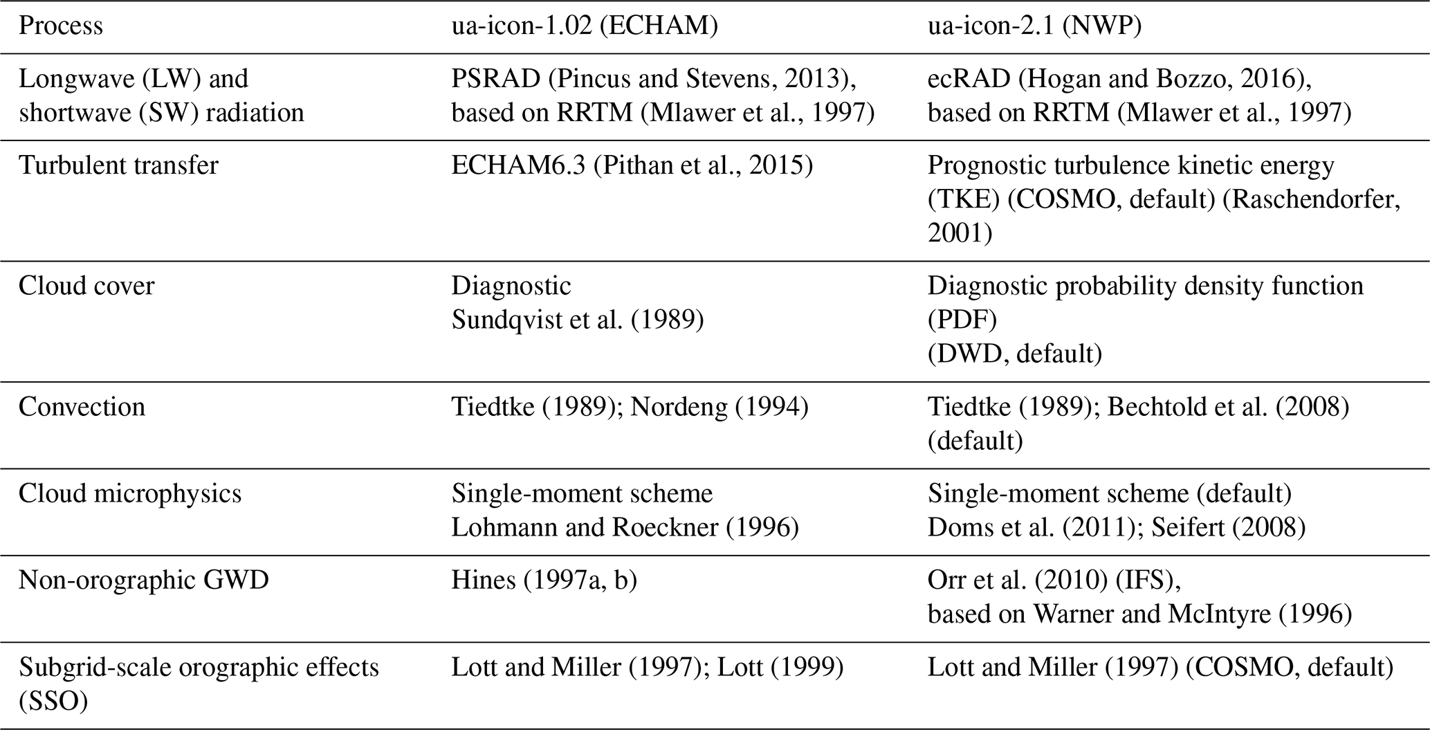
ICON is a joint development of the DWD, the MPI-M, the Deutsches Klimarechenzentrum (DKRZ), the Karlsruhe Institute of Technology (KIT), and the Center for Climate Systems Modeling (C2SM) to create a modeling framework that serves the need for NWP as well as the application for climate simulations. For these tasks, originally two physics packages with sets of parameterizations were available, i.e., NWP (Zängl et al., 2015) for weather prediction and ECHAM for climate applications (Giorgetta et al., 2018; Jungclaus et al., 2022). ICON employs a nonhydrostatic dynamical core on an unstructured triangular C grid as well as a geometric altitude grid that is terrain-following up to a certain height. Lorenz staggering is applied in the vertical, with the prognostic variables of the grid-edge-normal wind components, the potential temperature, and the density of moist air defined at full model levels and the vertical wind component defined at half levels. The main parameterizations of the NWP and ECHAM physics packages, as applied in this work, are listed in Table 1. ICON's UA extension consists of an optional deep-atmosphere dynamical core and supplementary physical parameterizations for the relevant physical processes in the MLT (Borchert et al., 2019). These are parameterizations for molecular diffusion (Huang et al., 1998), ion drag and Joule heating (Hong and Lindzen, 1976), frictional heating (Gill, 1982), heating rates of O₂ absorption of ultraviolet (UV) in the Schumann–Runge bands and continuum (Strobel, 1978), absorption of extreme UV by N₂, O, and O₂ (Richards et al., 1994), non-local thermodynamic equilibrium (non-LTE) infrared cooling by CO₂, NO, and O₃ (Fomichev and Blanchet, 1995; Fomichev et al., 1998; Ogibalov and Fomichev, 2003), and infrared NO cooling at 5.3 µm (Kockarts, 1980). UA-ICON does not include interactive chemistry and describes the chemical heating with a climatological annual cycle from a 30-year time slice simulation of HAMMONIA (Schmidt et al., 2006).

(Pincus and Stevens, 2013)(Mlawer et al., 1997)(Hogan and Bozzo, 2016)(Mlawer et al., 1997)(Pithan et al., 2015)(Raschendorfer, 2001)Sundqvist et al. (1989)Tiedtke (1989)Nordeng (1994)Tiedtke (1989)Bechtold et al. (2008)Lohmann and Roeckner (1996)Doms et al. (2011)Seifert (2008)Hines (1997a, b)Orr et al. (2010)Warner and McIntyre (1996)Lott and Miller (1997)Lott (1999)Lott and Miller (1997)

Table 1 Parameterizations for the physical processes given in the first column in UA-ICON simulations with ECHAM physics (second column) and the NWP physics package (third column).

The ICON release icon-2024.01-1 (ICON partnership (DWD, MPI-M, DKRZ, KIT, and C2SM), 2024) is the code basis in this work whenever using the NWP physics package (ua-icon-2.1). In contrast, the UA-ICON simulation using the ECHAM physics package is based on a slightly updated version of Borchert et al. (2019) (ua-icon-1.02). The model code used in this study is published on Zenodo (Kunze et al., 2024). It is based to a large extent on Fortran. We checked the code quality with FortranAnalyser (García-Rodríguez et al., 2024) and obtained a final score of 4.1, which is a relatively high score compared to the existing climate models (Michael García-Rodríguez, personal communication, 16 February 2025). The ICON model code is largely equipped with OpenACC directives, and in special configurations ICON has been deployed on GPU computing architectures (Giorgetta et al., 2022). However, the upper-atmospheric extension is not ported to the GPU, and we performed our model simulations on the CPU architecture of the DKRZ (German Climate Computing Center) high-performance-computing (HPC) system. Using the message-passing interface with 20 cores and 2560 processors, 1 year of simulation requires a wall-clock time of 62 min.

All simulations in this work use the R2B4 horizontal resolution, corresponding to a grid distance of ∼ 160 km and 120 levels up to 150 km. They all apply the UA extension of ICON described by Borchert et al. (2019) for the ECHAM and NWP physics packages.

Borchert et al. (2019)

Table 2 UA-ICON time slice simulations with a seasonal cycle, with the columns indicating the simulation's label, the version, the physics package, the number of years after a 1-year spinup, and the setup. Table 3 details the simulation's setup with NWP physics.

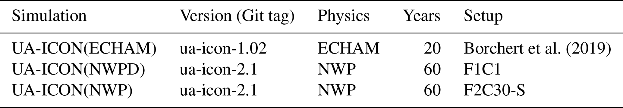
Three time slice simulations with a seasonal cycle are presented here with boundary conditions representative of the late 1990s, as listed in Table 2. The UA-ICON(NWP) simulations use repeated, seasonally varying climatological (1979–2016) conditions for the sea surface temperatures and sea ice concentrations from the Program for Climate Model Diagnosis and Intercomparison (PCMDI) Atmospheric Model Intercomparison Project (PCMDI-AMIP 1.1.2) dataset (Taylor et al., 2000). The radiatively active gases in ecRAD are prescribed as globally yearly averaged values (1990–2000) for CO₂ and modified with a tanh profile for CH₄, N₂O, CFC-11, and CFC-12. Tropospheric background aerosol optical properties, representing conditions of the year 1865, are prescribed for ecRAD (Kinne et al., 2013). The radiatively active gases for the upper-atmospheric extension, i.e., CO₂, NO, O₃, O₂, and O, and the O₃ for ecRAD are prescribed from a 35-year climatology of a HAMMONIA simulation (Schmidt et al., 2006). The solar forcing is constant, with 14 spectrally resolved irradiances and a total solar irradiance of 1361.12 W m⁻² averaged from 1979 to 2016, using the dataset prepared for CMIP6 (Matthes et al., 2017); the F10.7 cm solar flux for the calculation of the EUV heating rates is set to 150 sfu (1 sfu $=\mathrm{1}\times {\mathrm{10}}^{-\mathrm{22}}$ W m⁻² Hz⁻¹). The 20-year UA-ICON(ECHAM) simulation uses the same boundary conditions and settings as Borchert et al. (2019), while the UA-ICON(NWPD) and UA-ICON(NWP) simulations all use NWP physics. They are run for 60 years after 1 year of spinup. UA-ICON with NWP physics requires longer simulation periods than UA-ICON with ECHAM physics, e.g., for reliable conclusions concerning statistics based on major SSWs, as the dynamic variability is much higher. The second simulation, UA-ICON(NWPD), uses the default settings (therefore labeled NWPD) for the OGWD and NGWD parameterizations (label F1C1 in Table 3), and UA-ICON(NWP) uses tuned parameters for the OGWD and NGWD parameterizations (label F2C30-S in Table 3). The major features of ECHAM and NWP physics are summarized in Table 1. The difference in NGWD parameterization between the physics packages, Hines (1997a, b) (H97) in ECHAM and Warner and McIntyre (1996) (WM96) in NWP, has an especially substantial impact on the climatology of the MLT, which is emphasized in Sect. 3.

Table 3 Parameter setting of the WM96 NGWD (C^*, ${\mathit{\rho }}_{\mathrm{0}}\left|{\widehat{\mathit{F}}}_p\right|$) and the LM97 OGWD parameterizations of the tuning simulations in perpetual January mode. C^* is a factor to increase the saturation momentum flux density. ${\mathit{\rho }}_{\mathrm{0}}\left|{\widehat{\mathit{F}}}_p\right|$ is the total launch momentum flux in each azimuth (mPa). K_wake is the low-level wake drag constant. K_drag is the gravity wave drag constant. Fr_crit is the critical Froude number. All of the simulations use the same default settings for the WM96 tunable L_p=450 hPa, which is the launch height of the gravity wave spectrum. The setups NWPD and NWP are used for the UA-ICON(NWPD) and UA-ICON(NWP) simulations with a seasonal cycle.

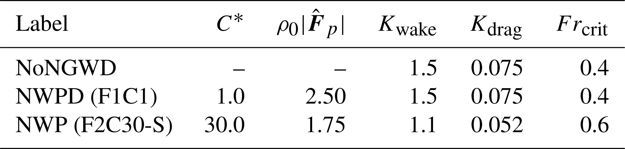
Table 3 gives the parameter values of the GWD parameterizations for the simulations discussed here. We have increased the scaling factor of the saturation momentum flux density (C^*) of WM96, introduced by McLandress and Scinocca (2005) when comparing the H97, WM96, and Alexander and Dunkerton (1999) NGWD parameterizations. The total launch momentum flux in each azimuth ($\mathit{\rho }\left|{\widehat{\mathit{F}}}_p\right|$) is reduced from its default value of 2.50 mPa to 1.75 mPa. The adaptations for the OGWD parameterization include changes in tunable parameters, i.e., the low-level wake drag constant (K_wake), the gravity wave drag constant (K_drag), and the critical Froude number (Fr_crit).

2.2 Reanalyses and satellite observations

We use the temperature and zonal wind of the three reanalyses ERA5 (Hersbach et al., 2020), NCEP/NCAR (Kalnay et al., 1996; Kistler et al., 2001), and MERRA-2 (Gelaro et al., 2017) for the evaluation of the NH stratospheric variability and the statistical evaluation of SSWs.

For the evaluation of the MLT temperature and zonal wind, we use the latest version (v2.07, v2.08 from December 2020 onward) of satellite observations from the SABER instrument on the TIMED (Thermosphere, Ionosphere, Mesosphere, Energetics and Dynamics) satellite (Russell III et al., 1999; Dawkins et al., 2018). The original Level-2A data, sorted by event and altitude, are binned to a regular latitude-by-altitude grid with a temporal resolution of 1 month and a spatial resolution of 5° horizontally and 1 km vertically. As a reference for the zonal mean zonal wind in the MLT, we use data from the UARS (Upper Atmosphere Research Satellite) Reference Atmosphere Project (URAP) (Swinbank and Ortland, 2003). For daily resolved temperature observations through the middle atmosphere, including the MLT region, we use Aura Microwave Limb Sounder (Aura-MLS) version 5.0 Level-3 data at pressure levels (Livesey et al., 2022).

2.3 Methods

The original UA-ICON output data are stored instantaneously on the R2B4 triangular grid with an output frequency of 6 h for the basic dynamical quantities. Additionally, temperature, pressure, and zonal and meridional wind components are output instantaneously at a 1 h frequency for the analyses of tidal activity. The model daily averaged tendencies of the physical parameterizations are output with a frequency of 1 d. These triangular output data are transferred to a regular Gaussian grid with 192 longitudes and 96 latitudes (T63) and 120 fixed geometric altitude levels, corresponding to the model full height levels once the influence of the orography levels off for the postprocessing procedures. The so-called transformed Eulerian mean (TEM) quantities (Andrews and McIntyre, 1976; Andrews et al., 1987), i.e., the Eliassen–Palm (EP) diagnostics, which are the EP flux (F) and its divergence (∇⋅F) and the meridional and vertical components of the residual mean meridional circulation (MMC) (${\stackrel{\mathrm{‾}}{v}}^{*}$ and ${\stackrel{\mathrm{‾}}{w}}^{*}$), are calculated on the 120 height levels of the T63 grid. We use the formulation of the hydrostatic primitive equations (HPEs) on the geometric coordinates, HPE(z), of Hardiman et al. (2010) for the computation of the EP diagnostics. Hardiman et al. (2010) demonstrated the large error made when calculating the EP diagnostics based on the formulation of the HPEs on the log-pressure coordinates, HPE(ln(p)), for nonhydrostatic models formulated at geometric altitude levels. For the analysis of major sudden stratospheric warmings and the related diagnostics of mesospheric coupling, the daily UA-ICON output is vertically interpolated to a set of 53 standard pressure levels. This allows a more direct comparison with the reanalysis products and other related published benchmarks.

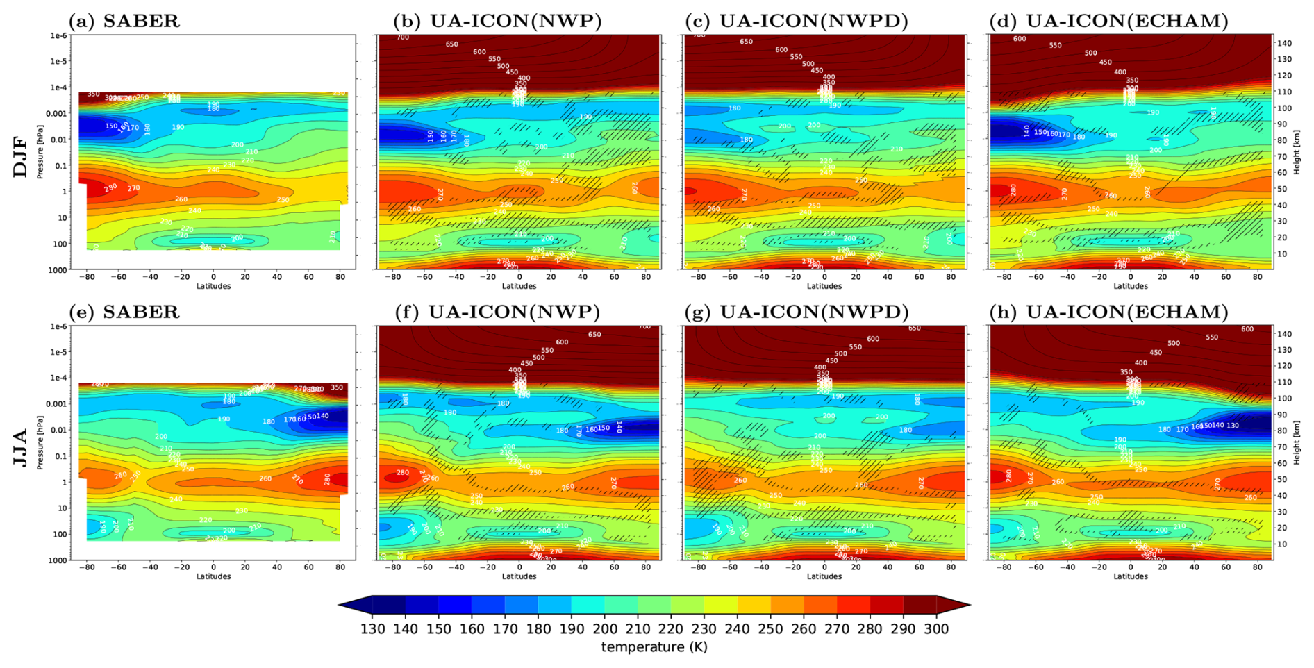
Figure 1 Climatology of the zonal mean temperature for the December–January–February (a–d) and June–July–August (e–h) seasonal mean. (a, e) SABER (2002–2022). (b, f) UA-ICON with NWP physics and tuned gravity waves (F2C30-S in Table 3). (c, g) UA-ICON with NWP physics (default settings, F1C1 in Table 3). (d, h) UA-ICON with ECHAM physics. In the hatched areas the UA-ICON simulations are not statistically different to SABER based on the 95 % confidence level.

3 Global circulation

Shortcomings in the UA-ICON(NWPD) (with default settings) climatology of the MLT are the main motivation for a re-tuning of the NGWD and OGWD parameterizations in UA-ICON(NWP). We compare the zonal mean temperature (Fig. 1) and zonal mean zonal wind (Fig. 2) in the boreal and austral winter seasons from UA-ICON to SABER and URAP climatologies. Comparing UA-ICON(NWP) with its default parameter settings for the GW parameterizations, chosen for the standard version up to ∼ 75 km (Figs. 1 and 2c, g, in the following abbreviated with UA-ICON(NWPD)) with temperature from SABER (Fig. 1a, e) and the URAP zonal wind (Fig. 2a, e), we can identify the deficits in the MLT region, with a warm temperature bias in the summer mesopause region of more than 30 K, an eastward zonal mean zonal wind extending from the middle atmosphere to the lower thermosphere during the winter seasons, and a westward zonal mean zonal wind during the summer seasons reversing only slightly to an eastward direction at altitudes from 100 to 110 km. We significantly reduce these deficits of UA-ICON(NWPD) in the MLT region for the temperature and the zonal wind using the tuned parameters for the OGWD and NGWD parameterizations of UA-ICON(NWP) (Figs. 1 and 2b, f). The temperature in the austral and boreal summer MLT region decreases by more than 30 K in UA-ICON(NWP), which is now comparable to SABER (Fig. 1a, e) during the austral and boreal summer seasons, whereas UA-ICON(ECHAM) shows a cold bias of 10 K in this region for both seasons (Fig. 1d, h). The reversals from the westward-directed summer zonal mean zonal wind in the middle atmosphere to an eastward zonal wind direction in the upper mesosphere are present in UA-ICON(NWP) (Fig. 2b, f) with a magnitude higher than that of URAP (Fig. 2a, e), whereas UA-ICON(ECHAM) (Fig. 2d, h) shows a wind reversal too intense and too low in altitude, as reported by Borchert et al. (2019). This effect of the NGWD tuning on UA-ICON(NWP) limits the mesospheric polar vortex to an altitude of ∼ 80 km, whereas in both winter seasons it extends to an altitude of approximately 100 km in the URAP climatology. Comparable differences were reported, e.g., by Harvey et al. (2019) in modeling the extension of the mesospheric polar vortex with WACCM although specifying the dynamics to an altitude of 60 km from MERRA-2 data. The winter westerly winds at high latitudes in WACCM extend to lower altitudes, compared to geostrophic zonal winds calculated from SABER-derived geopotential heights. The magnitude of the eastward-directed zonal winter circulation in the middle atmosphere is too high in the Southern Hemisphere (SH) in UA-ICON(NWP) by 20 m s⁻¹ and slightly too high in the NH. However, the position of the westerly jets is captured well in both hemispheres compared to URAP. A second side-effect of increasing the eastward-directed NGWD in UA-ICON(NWP) is the weakening of the westward-directed zonal circulation in summer, leading to a shift in the −30 m s⁻¹ contour to lower latitudes by more than 10° in the upper mesosphere. The magnitude of the NH summer westward-directed zonal circulation (≤50 m s⁻¹) compares well with URAP. However, the location of this easterly jet is too low in altitude and is shifted too far to low latitudes. This shift in the easterly jet also appears in the SH summer, together with a slightly too strong westward-directed zonal circulation (≤60 m s⁻¹).

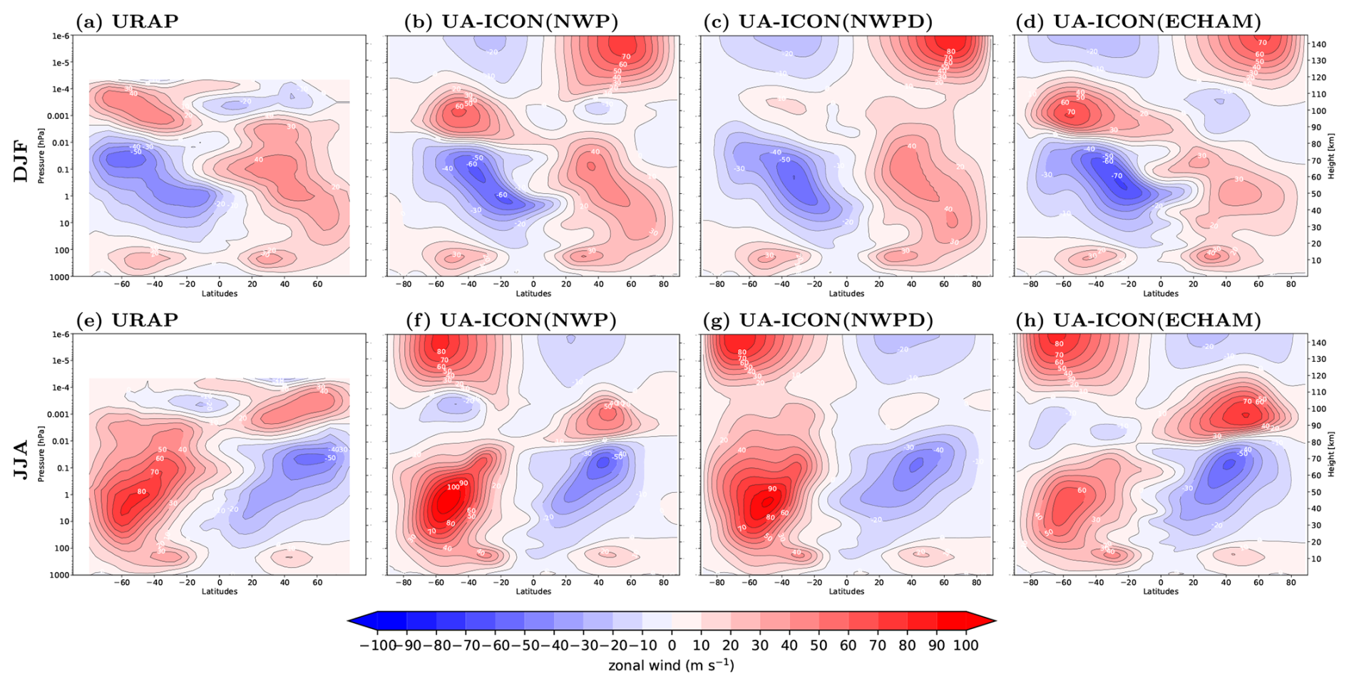
Figure 2 Climatology of the zonal mean zonal wind for the December–January–February (a–d) and June–July–August (e–h) seasonal mean. (a, e) URAP climatology. (b, f) UA-ICON with NWP physics and tuned gravity waves (F2C30-S, in Table 3). (c, g) UA-ICON with NWP physics (default settings, F1C1 in Table 3). (d, h) UA-ICON with ECHAM physics.

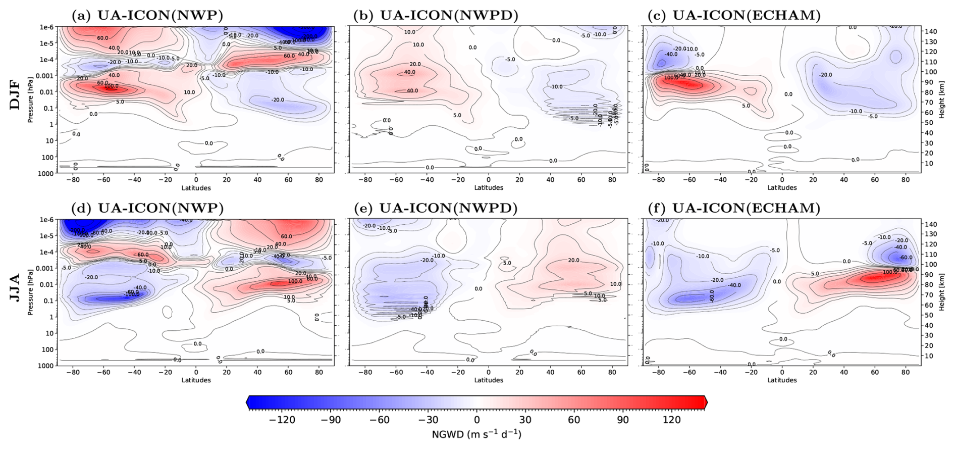
Figure 3 Multiyear boreal (a–c) and austral (d–f) winter seasonal zonal mean zonal wind tendencies (m s⁻¹ d⁻¹) due to non-orographic gravity waves of UA-ICON simulations with NWP physics (Warner and McIntyre, 1996) with tuned gravity waves (a, d), NWP physics with default gravity wave parameters (b, e), and ECHAM physics (Hines, 1997a, b) (c, f).

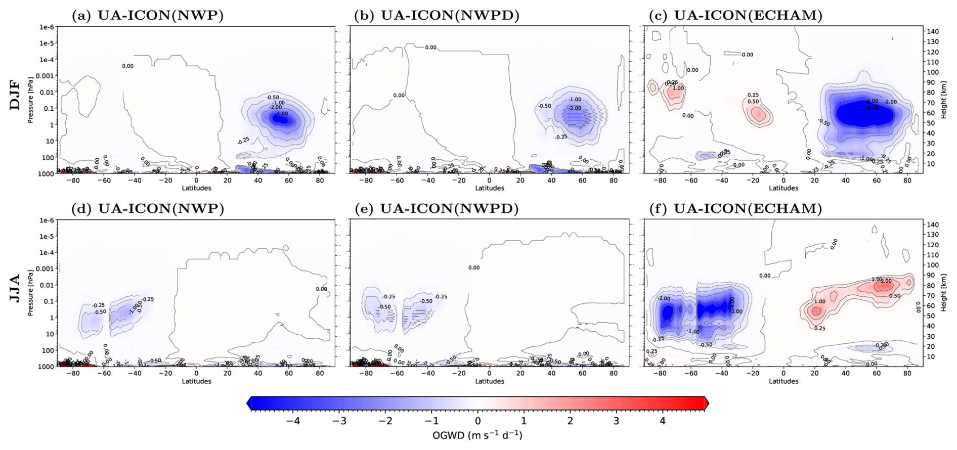
Figure 4 Multiyear boreal (a–c) and austral (d–f) winter seasonal zonal mean zonal wind tendencies (m s⁻¹ d⁻¹) due to orographic gravity waves of UA-ICON simulations with NWP physics (Lott and Miller, 1997) with tuned non-orographic gravity waves (a, d), NWP physics with default gravity wave parameters (b, e), and ECHAM physics (Lott, 1999) (c, f).

UA-ICON(ECHAM) and UA-ICON(NWPD) have a warm bias in winter stratopause temperature compared to SABER, which intensifies by the tuning of the NGWD parameterization in UA-ICON(NWP). However, the winter stratospheric temperature is in better agreement with SABER for both UA-ICON(NWP) and UA-ICON(NWPD), and the strength of the Northern Hemisphere stratospheric vortex is much better captured compared to URAP. In general, using ICON with the NWP physics package leads to a much better representation of the stratosphere that eliminates the problems with the stratospheric circulation and temperatures in ICON(ECHAM) noticed by Giorgetta et al. (2018) and in UA-ICON(ECHAM) noticed by Borchert et al. (2019). However, overall, the differences in zonal mean temperature between all of the UA-ICON simulations and SABER are significant in most areas, as indicated by the non-hatched areas in Fig. 1. The same holds for the zonal mean wind compared to ERA5, where all UA-ICON simulations show significant differences in most areas up to 80 km in altitude (not shown).

The main driver of the mesosphere global circulation is the breaking of NGWs (e.g., Becker, 2012, Vincent, 2015, and references therein) that force a meridional circulation from the summer hemisphere to the winter hemisphere, downwelling and adiabatic warming over the winter pole, and upwelling in the summer mesosphere, leading to adiabatic cooling with temperatures far below the radiative equilibrium. The coarse resolution of the UA-ICON simulations in the present work does not allow for explicit resolution of the upward propagation and breaking of NGWs. Therefore, the effects of NGWs are parameterized according to H97 in UA-ICON(ECHAM) and based on WM96 in UA-ICON(NWP). Figure 3 shows the zonal mean zonal wind tendencies due to the parameterized NGWD. Compared to the H97 tuning, with more than 130 m s⁻¹ d⁻¹ in both winter seasons at an altitude between 80 and 100 km (Fig. 3c, f), WM96, with NWP default settings, shows much smaller tendencies of only up to 40 m s⁻¹ d⁻¹ in the SH winter or 24 m s⁻¹ d⁻¹ in the NH winter (Fig. 3b, e). This missing NGWD in the MLT is mainly responsible for the large discrepancies in climatological zonal mean zonal wind and temperatures as present in UA-ICON(NWPD) (Figs. 2 and 1c, g), and by increasing the NGWD of WM96 in the MLT to values comparable to H97 (Fig. 3a, d), the temperature and zonal wind in the MLT improve considerably (Figs. 1 and 2b, f). The latitudinal structure of the zonal wind tendencies from H97 and WM96 up to an altitude of 100 km are very similar. This similarity is the result of increasing the saturation momentum flux density of WM96, as proposed by McLandress and Scinocca (2005), by a factor of 30 (see Sect. 4 for more details). Both physics packages in ICON use the parameterization based on Lott and Miller (1997) (LM97) to account for the OGWD. However, the ECHAM physics package uses the implementation of ECHAM6 (Lott, 1999), whereas NWP physics uses the COSMO implementation. OGWD mainly acts in the stratosphere, and the resulting zonal mean zonal wind tendencies show relatively huge differences of up to a factor of 4, with a larger OGWD in UA-ICON(ECHAM) (Fig. 4c, f) than in UA-ICON(NWPD) (Fig. 4b, e) and UA-ICON(NWP) (Fig. 4a, d). The parameters of the OGWD parameterization in UA-ICON(NWP) are adapted for the coarser R2B4 horizontal resolution of UA-ICON as listed in Table 3 (F2C30-S). Using this, the OGWD increases in the NH middle atmosphere in winter by a factor of 2 (UA-ICON(NWP), Fig. 4a), whereas there are only minor changes in June–July–August (JJA) (Fig. 4d).

4 Gravity wave tuning

The tuning parameters applied in the UA-ICON(NWP) simulation are the result of a series of perpetual January simulations (Table S1 in the Supplement) with variations of C^* of WM96. The total launch momentum flux in each azimuth ($\mathit{\rho }\left|{\widehat{\mathit{F}}}_p\right|$) is tested with its default value of 2.50 mPa and compared with 1.75 mPa, and the launch height (L_p=450 hPa) stays with its default value. The NWP simulation includes changes in the tunable parameters of the OGWD parameterization. Detailed results of these tuning simulations are documented in the Supplement to this paper. Table 3 gives a subset of the simulations discussed here, with a focus on the effects of switching off the WM96 NGWD completely (NoNGWD) and the final changes in the parameter settings of the WM96 and LM97 parameterizations (NWP) compared to the default settings (NWPD) (Fig. 5).

By switching off the WM96 NGWD completely (NoNGWD), we can evaluate the effect of the parameterized NGWs, shown with the latitude–altitude sections (Fig. 5) of the anomalies NoNGWD minus NWPD (left column). NoNGWD shows a strong response for all quantities, with the summer mesopause being too high in altitude and temperatures lower than the default (NWPD) case. The SH easterly wind regime extends to the lower thermosphere, and the meridional component of the residual MMC (${\stackrel{\mathrm{‾}}{v}}^{*}$), the northward-directed summer-to-winter circulation, is more intense and shifted to higher altitudes, peaking between 100 and 120 km globally. The EP flux divergence (∇⋅F) reflects the forcing of the zonal mean zonal wind by resolved waves. The NoNGWD simulation shows ∇⋅F to be more intense and in the opposite direction to NWPD, indicating an increase in dissipating resolved waves. These are the resolved waves with an eastward-directed phase speed, which can propagate to considerably higher altitudes in the easterly wind regime, extending to the MLT region in the SH. The NWP simulation, with an increasing C^* and a smaller $\mathit{\rho }\left|{\widehat{\mathit{F}}}_p\right|$, shows better results in the MLT. The parameterized WM96 NGWD increases by increasing the saturated momentum flux density from its default $C^{*}=\mathrm{1}$ to $C^{*}=\mathrm{30}$, which effectively increases the altitude where the upward-propagating NGWs dissipate, with a direct impact on the tendency of the zonal wind in the MLT region calculated by the NGWD parameterization (Fig. 5d). The anomalies indicate an increase in the weak eastward-directed NGWD of 40 m s⁻¹ d⁻¹ in the SH of the default (NWPD; Fig. 5d, left and Fig. 3b) by 100 to 140 m s⁻¹ (NWP; Fig. 5d, right and Fig. 3a) within a shallow layer, peaking near 81 km. Near 100 km, the NGWD changes to a westward direction in NWP in a layer up to about 120 km and turns again to an eastward direction. Increasing the eastward-directed NGWD in the SH upper mesosphere accelerates the zonal mean zonal wind in the SH MLT by more than 50 m s⁻¹ (Fig. 5b, right) and intensifies the MMC, as indicated by the stronger northward-directed summer-to-winter ${\stackrel{\mathrm{‾}}{v}}^{*}$ near an altitude of 80 km (Fig. 5c, right). The forced upwelling at high latitudes in the SH leads to adiabatic cooling in the MLT, peaking with −50 K in a layer from 80 to 90 km (Fig. 5a, right). Above 100 km, the MMC turns to a southward-directed flow with increasing C^*, which is directly related to the more westward-directed NGWD-induced zonal wind changes in the SH and the change to an eastward-directed NGWD in the NH. This winter–summer-directed flow extends over both hemispheres in a layer between 100 and 120 km, with a minimum near the Equator. Qian et al. (2017) and Wang et al. (2022) reported similar features for SD-WACCM simulations and compared them to the MMC derived from vertical gradients of the SABER CO₂ volume mixing ratio. They found large vertical CO₂ gradients in the 95–110 km height region at summer hemispheric polar latitudes, consistent with the SD-WACCM CO₂ gradients as well as the upward-directed residual flow in the upper mesosphere and the downward-directed residual flow of the lower thermosphere.

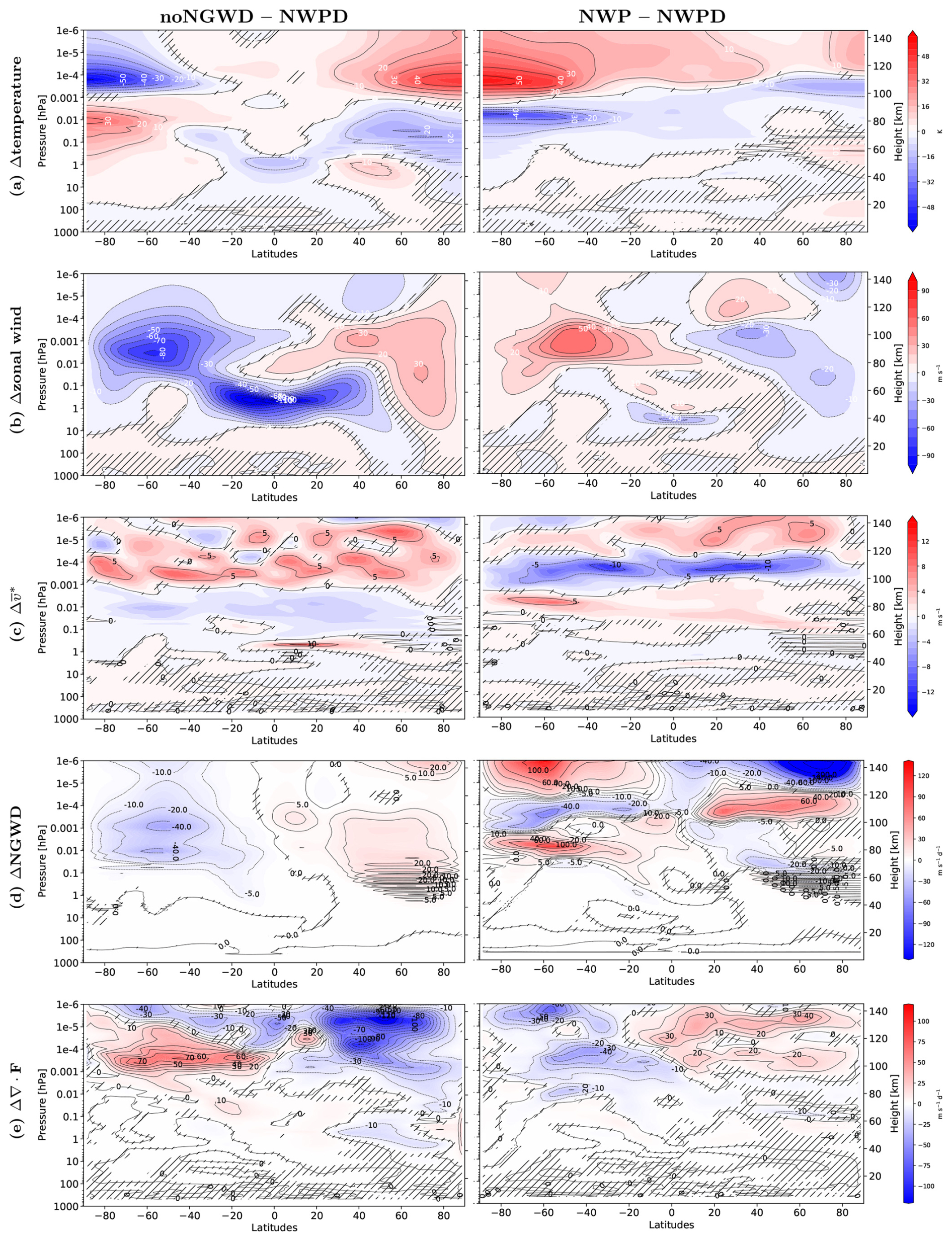
Figure 5 Perpetual January zonal mean long-term mean anomalies calculated with respect to NWPD (F1C1) for NoNGWD (left row) and NWP (F2C30-S) (right row). (a) Temperature (K). (b) Zonal wind (m s⁻¹). (c) Transformed Eulerian mean meridional velocity (${\stackrel{\mathrm{‾}}{v}}^{*}$) (m s⁻¹). (d) Zonal wind tendency due to non-orographic gravity waves (m s⁻¹ d⁻¹). (e) Divergence of the Eliassen–Palm vector (∇⋅F) (m s⁻¹ d⁻¹). In the hatched areas the anomalies are not statistically significant, based on the 95 % confidence level.

The significant NGWD changes in the NH contribute to decelerating the eastward-directed polar night jet in the upper mesosphere, whereas the zonal wind changes around the stratopause are due to the more intense westward-directed OGWD (see Fig. 4a, b).

Derived from the numerical experiments, one parameter setup in Table 3, NWP (F2C30-S), corresponding to $C^{*}=\mathrm{30}$ and an adaptation of the OGWD parameters, provides the most reasonable prediction and therefore is used for further investigations in the time slice simulation UA-ICON(NWP) in Table 2. This version best reproduces a reasonably strong westerly stratospheric jet and an easterly mesospheric jet in the Northern Hemisphere as well as their reversed counterparts in the Southern Hemisphere, together with a reasonably low temperature in the summer mesopause region.

5 Northern Hemisphere stratospheric and mesospheric winter variability

The process of parameter optimization (tuning) presented in Sect. 4 has been carried out with a clear focus on the climatological state of the MLT, where the parameter-optimized simulation UA-ICON(NWP) shows a clear improvement. However, parameter optimizations otherwise potentially worsen the model performance in other regions of the atmosphere, e.g., as discussed for the warm stratopause temperature bias. In this section, we focus on the NH stratospheric and mesospheric winter variability in order to evaluate the implication of the parameter optimization for this important dynamical aspect of the model. A key measure of the NH winter variability is the frequency of major SSWs, which is closely related to troposphere–stratosphere coupling via the upward propagation of planetary wave and gravity wave activity (Sect. 5.2).

5.1 Seasonal cycle of Northern Hemisphere stratospheric variability

Figure 6 shows the climatological seasonal cycle of NH stratospheric (10 hPa) polar temperature and mid-latitude (near 60° N) zonal wind for UA-ICON(ECHAM), UA-ICON(NWPD), UA-ICON(NWP), and ERA5 (1963–2022) with the solid black line. Overlaid with lighter shading are the daily mean maxima and minima occurring within the 60 years (20 years for UA-ICON(ECHAM)) in each dataset. The overlaid darker shading gives the ±1 range of the standard deviation of the daily averaged time series. Figure 7 shows the deviations of the climatological seasonal cycles presented in Fig. 6 for the UA-ICON simulations compared to ERA5. We start with a discussion of the daily climatological time series (solid black line in Fig. 6) and the deviations of the UA-ICON simulations to ERA5 (Fig. 7). The summer temperatures are too warm by ∼ 4 K for UA-ICON(ECHAM), ∼ 1 K for UA-ICON(NWP), and ∼ 2 K for UA-ICON(NWPD) compared to ERA5. With the transition to the westerly circulation in October, the warm biases of both UA-ICON(ECHAM) and UA-ICON(NWP) get larger, reaching a maximum of 11–16 K in December. The warm bias of the tuned UA-ICON(NWP) simulation is slightly larger in early winter. This larger dynamic heating is probably due to a stronger orographic GWD. By the middle to end of December, these positive anomalies are outside the 99 % confidence interval of the daily ERA5 North Pole temperature, which is given with the light-green shading around the zero line in Fig. 7, indicating a significant warm bias in the NH polar stratosphere. On average, the warm biases for the UA-ICON(NWP) and UA-ICON(ECHAM) simulations decrease in January and February, fluctuating around 2–3 K, whereas UA-ICON(ECHAM) in March and April shows good agreement with ERA5 and the warm bias of UA-ICON(NWP) increases. The good agreement of the UA-ICON(ECHAM) simulation in 10 hPa NH polar temperatures from January to April with ERA5 is partly a consequence of the weak intensity of the SSWs in this simulation, as seen in the weak variability. Both the ERA5 and UA-ICON(NWP) simulations show intense increases in polar 10 hPa temperature during SSWs, especially in the late winter period, contributing to an increase in the climatological mean. The 10 hPa zonal mean zonal wind near 60° N is slightly too strong for UA-ICON(NWP) simulations during the summer season, whereas UA-ICON(ECHAM), at least from late July to the beginning of September, is very close to ERA5. However, beginning with the transition to the westerly circulation, UA-ICON(ECHAM) shows weak zonal winds, with deviations to ERA5 peaking at −25 m s⁻¹ in late December. All UA-ICON(NWP) values are in better agreement with ERA5 during the NH winter season. Both UA-ICON(NWP) simulations show in October to December moderate deviations of the zonal mean zonal wind to ERA5, most of the time within or close to the ERA5 confidence interval. Later in winter, from January to March, the zonal wind of UA-ICON(NWPD) exceeds the zonal wind in ERA5 by up to 15 m s⁻¹ and by 5–12 m s⁻¹ for UA-ICON(NWP), most of the time outside the ERA5 confidence interval. Regarding the winter variability, presented with the daily extremes and the range of ± 1 standard deviation in Fig. 6, all of the UA-ICON(NWP) simulations show far better performance than UA-ICON(ECHAM). The observational record of the NH stratospheric winter variability, given with ERA5 (Fig. 6a, b, right), indicates an increase in temperature maxima near the North Pole in December. This is accompanied by the occurrence of easterly extremes which indicate major SSW events. SSWs tend to be more intense and occur more often during January and February, as reflected by the warmest maxima and the most intense easterlies in these months. The UA-ICON(ECHAM) (Fig. 6a, b, left) simulation shows a much lower NH stratospheric winter variability characterized by the smaller standard deviations of the wind and the temperature difference and the less pronounced extreme values, compared to the UA-ICON(NWPD) and UA-ICON(NWP) simulations. However, due to the weak zonal mean wind, easterly winds occur and the criteria for SSWs are fulfilled frequently. In both UA-ICON(NWP) simulations, the range of maxima and minima is comparable to ERA5. Regarding the timing of the most extreme temperature and zonal wind anomalies, both UA-ICON(NWP) simulations show SSW-related extremes too early in November and too late in March. However, there are fewer easterly extremes in mid-winter than in ERA5.

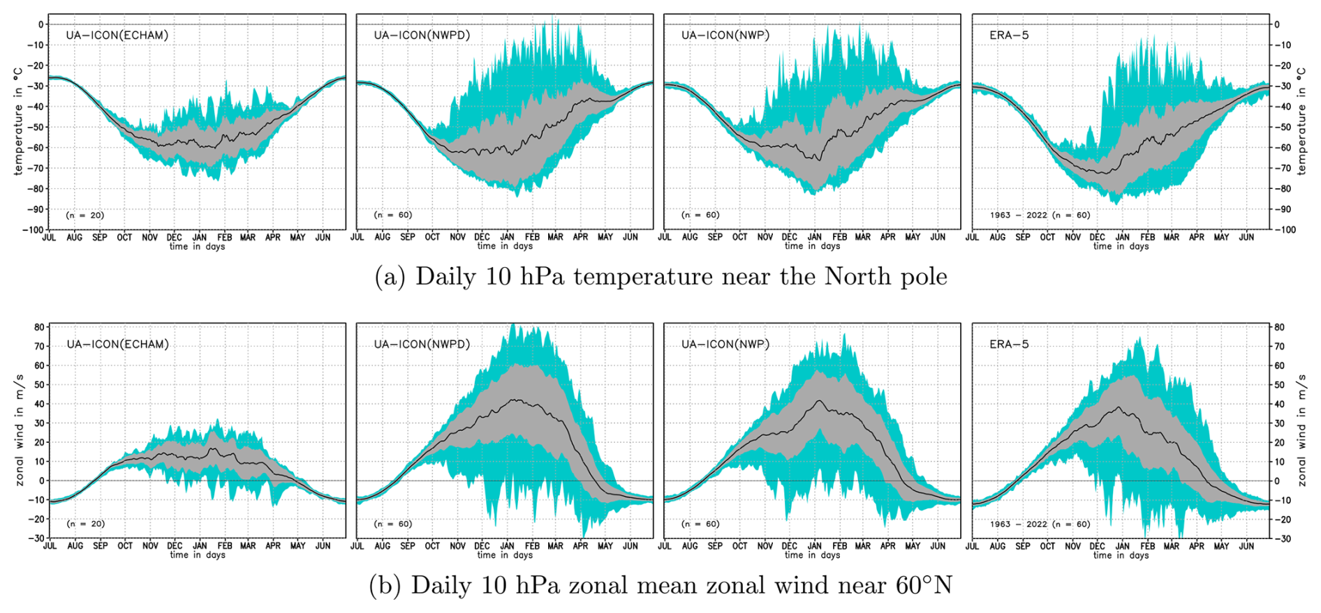
Figure 6 Climatological seasonal cycle of the daily 10 hPa temperature near the North Pole. (b) Zonal mean zonal wind near 60° N for the UA-ICON simulations and ERA5. From left to right: UA-ICON(ECHAM), UA-ICON(NWPD), UA-ICON(NWP), and ERA5 (1963–2022). The solid black line indicates the long-term averaged daily mean time series, the darker shading indicates a range of ±1 standard deviation around the average, and the lighter shading indicates the maxima or minima reached within the complete daily datasets.

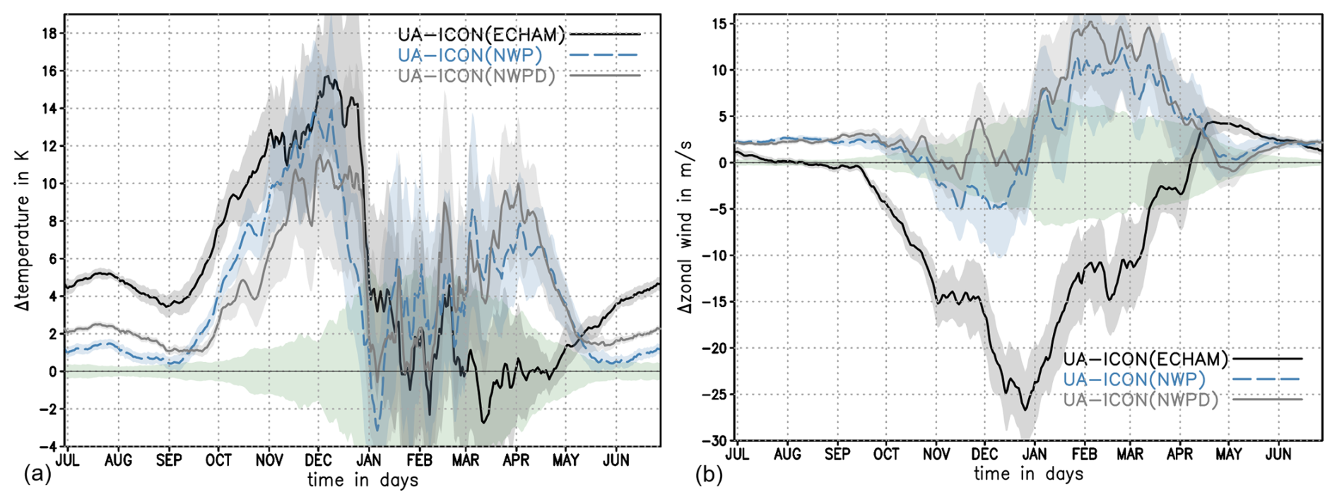
Figure 7 Climatological seasonal cycle of daily deviations of the UA-ICON simulations from ERA5. (a) The 10 hPa temperature near the North Pole. (b) The 10 hPa zonal mean zonal wind near 60° N. The shading represents the 99 % confidence interval of the individual simulations' daily mean. The light-green shading around the zero line indicates the 99 % confidence interval of the ERA5 data.

5.2 Major sudden stratospheric warmings

Major SSWs are accompanied by changing mesospheric and thermospheric propagation conditions for large-scale Rossby and gravity waves and tides. The mechanism is further illustrated in Fig. 8 with the time–height section of the averaged daily evolution of area-weighted averaged quantities centered at day 0 for SSW events detected in UA-ICON(NWP). Figure 8 (left) shows the absolute values of the quantities, whereas the right column shows the respective anomalies of the long-term daily mean. The zonal mean zonal wind (averaged from 50 to 70° N) (Fig. 8c, d) is decelerated in the stratosphere by Rossby waves with westward-propagating intrinsic phase speeds, focusing on the polar cap as represented by the strong convergence of the EP flux ∇⋅F (averaged from 70 to 90° N) (Fig. 8e, f) before day 0 of the SSWs, exerting a strong westward-directed drag on the zonal flow. The usual eastward-directed stratospheric flow allows the upward propagation of westward-propagating NGWs and OGWs, creating a westward-directed drag in the stratosphere and lower mesosphere (OGWD) and in the mesosphere (NGWD), as shown with the polar cap (70–90° N) averaged NGWD (Fig. 8g, h) and OGWD (Fig. 8i, j). With the onset of the westward-directed flow in the stratosphere, the filter conditions for the upward-propagating waves change and the Rossby waves and westward-propagating gravity waves are blocked, while eastward-propagating NGWs are now in favor of propagating upward. This is illustrated by the average time evolution of the wave drags around day 0 of SSWs in Fig. 8. A strong increase in negative ∇⋅F (convergence) starts some days before day 0 in the upper stratosphere and propagates downward. The EP flux diagnostic ∇⋅F not only accounts for large-scale planetary waves but also includes the other scales of the model that are related to resolved gravity waves, e.g., the westward-directed drag emerging in the upper stratosphere or lower mesosphere after day 0. A westward-directed (negative) planetary wave drag of up to 100 km has been found in several model simulations (Zülicke and Becker, 2013; Limpasuvan et al., 2016; Okui et al., 2021) as a result of baroclinic or barotropic instability (Sato and Nomoto, 2015). The persistent positive ∇⋅F (divergence) in the lower thermosphere near 110 km before and after the SSWs is related to eastward-propagating resolved waves. The reason for the appearance in a focused layer around 110 km in UA-ICON is most likely the particular vertical structure of incorporated WM96 NGWD parameterization. The westward-directed NGWD and OGWD decrease towards day 0. In the case of the NGWD, it turns eastward, starting in the upper mesosphere near day 0 and propagating downward near 10 hPa within 45 d. These strong changes in the wave forcing associated with SSWs have a large impact on the residual circulation, as shown by the polar cap (70–90° N) average of the meridional (Fig. 8k, l, $\stackrel{\mathrm{‾}}{v^{*}}$) and vertical (Fig. 8m, n, $\stackrel{\mathrm{‾}}{w^{*}}$) components of the residual MMC. On average, under NH winter conditions, $\stackrel{\mathrm{‾}}{v^{*}}$ is northward-directed (positive) and strongest in the lower mesosphere (60–70 km). In the course of SSW events, the mesospheric northward-directed $\stackrel{\mathrm{‾}}{v^{*}}$ weakens or even reverses to a southward-directed (negative) flow, whereas the northward-directed $\stackrel{\mathrm{‾}}{v^{*}}$ intensifies in the stratosphere. Consistently, for continuity reasons, the average NH winter conditions of downwelling (negative $\stackrel{\mathrm{‾}}{w^{*}}$) in the stratosphere and mesosphere change to an upward-directed flow in the lower mesosphere and an intensification of the downwelling in the stratosphere. The related anomalies of $\stackrel{\mathrm{‾}}{v^{*}}$ and $\stackrel{\mathrm{‾}}{w^{*}}$ (Fig. 8l, n) emphasize the outlined SSW-related changes in the residual MMC which are directly related to the induced adiabatic temperature changes with strong warming in the stratosphere, strong cooling in the mesosphere, and again warming in the lower thermosphere (Fig. 8a, b).

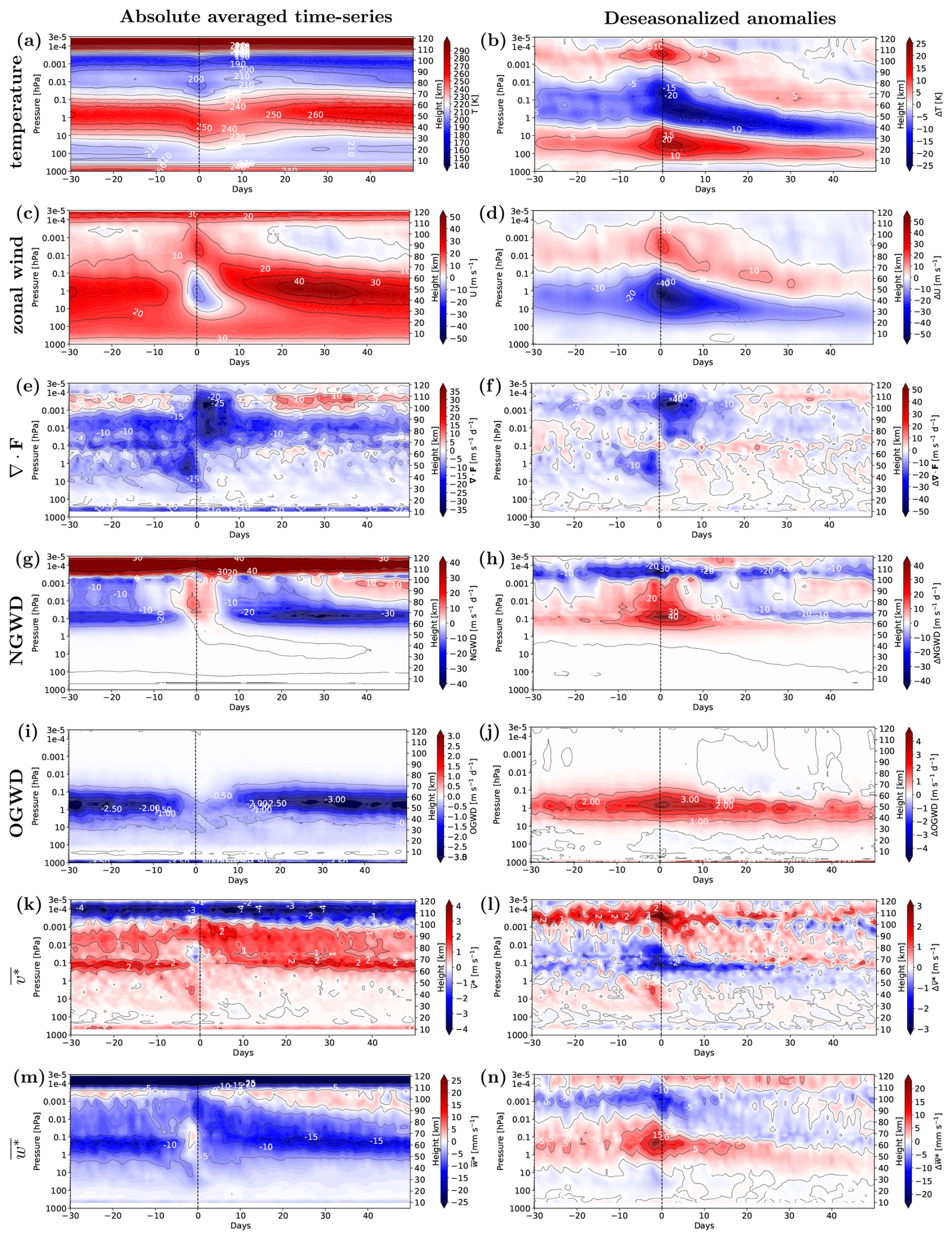
Figure 8 Time–height section of the UA-ICON(NWP) daily evolution of averaged quantities in a period around SSW events (left), with the associated anomalies of the averaged quantities relative to the respective long-term daily mean (right). At day 0 (the central day, vertical dashed line), the WMO criterion at 10 hPa for major SSWs is fulfilled for the first time.

To detect major SSWs, we apply the so-called WMO criterion (Mcinturff, 1978; Labitzke, 1981). According to this, two conditions need to be met at a pressure level of 10 hPa, reversing the climatological winter conditions in the middle stratosphere: (I) the zonal average zonal wind at 60° N (${\stackrel{\mathrm{‾}}{U}}_{\mathrm{60}\mathrm{N}}$) has to be in a westward direction (easterly wind), and (II) the difference in temperature between the zonal average at 60° N and the North Pole ($\stackrel{\mathrm{‾}}{\mathrm{\Delta }T}$) has to be positive within a time window of ±5 d around the central day of the SSW, which is the first day when condition I is fulfilled. The detection algorithm requires at least 20 d of westerly ${\stackrel{\mathrm{‾}}{U}}_{\mathrm{60}\mathrm{N}}$ between two SSWs and at least 10 d of westerlies preceding an SSW, with at least 1 d exceeding the threshold of 5 m s⁻¹. With these additional constraints, we avoid counting one SSW twice and distinguish final warmings from SSWs. Charlton and Polvani (2007) introduced the 20 d, based on the calculation of thermal damping times by Newman and Rosenfield (1997), a period that approximates two radiative timescales at 10 hPa.

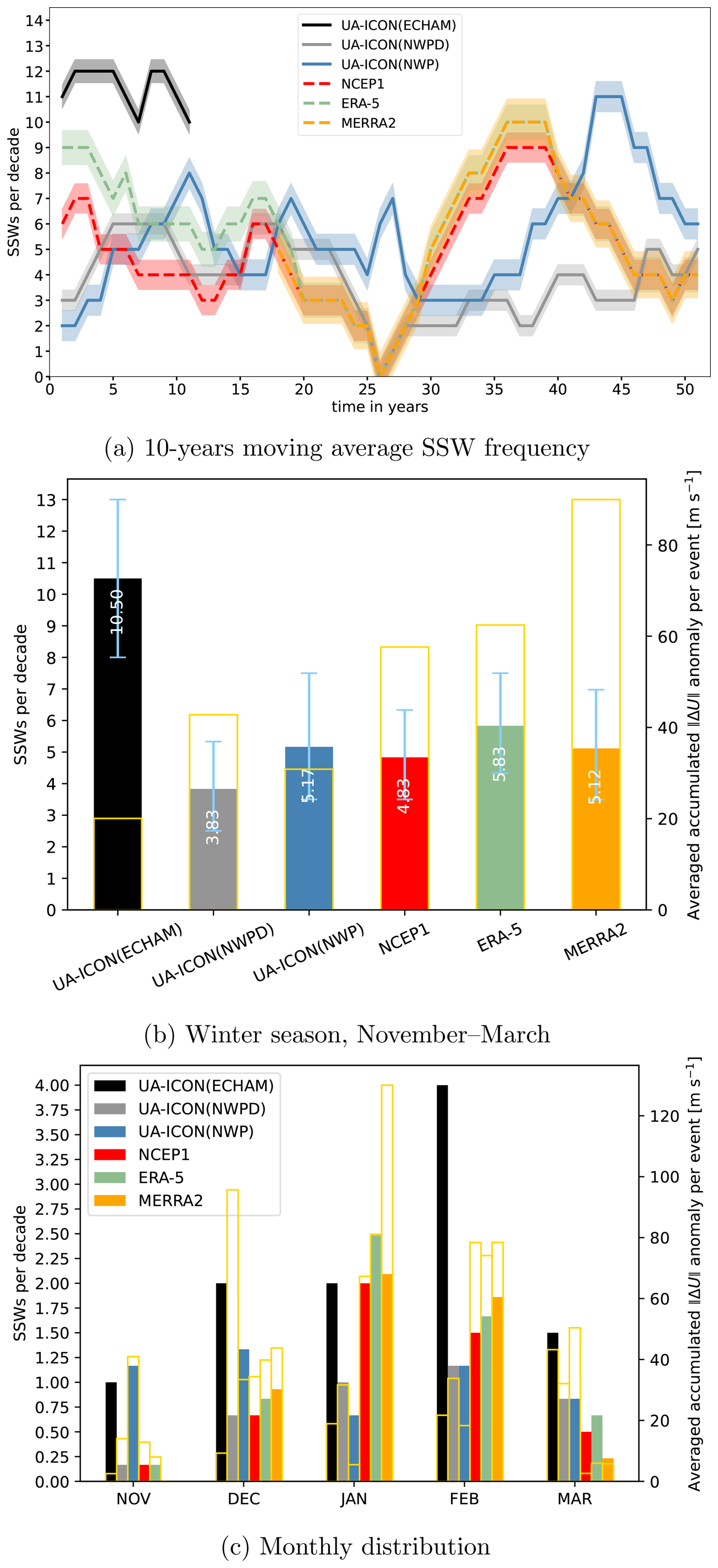
Figure 9 (a) Time series of the 10-year moving-average major SSW frequency in events per decade within the NH winter season (November–March) for UA-ICON simulations and reanalyses. The shading indicates the 95 % confidence interval. (b) Bar chart of SSWs per decade, with the error bars indicating the 95 % confidence interval. (c) The monthly distribution of SSWs per decade. The statistics are based on periods of 20 years for UA-ICON(ECHAM); 60 years for UA-ICON(NWPD), UA-ICON(NWP), NCEP1, and ERA5 (1963–2022); and 23 years for MERRA-2 (1980–2022).

There is substantial variability in the number of SSWs detected per decade (Fig. 9a), and the SSW frequency reported in the literature is therefore dependent on the analysis period, in addition to the criterion applied for the SSW detection (Butler et al., 2015). The value of six SSWs per decade, frequently reported (e.g., Charlton and Polvani, 2007; Butler et al., 2017), refers to SSW detection based on the 10 hPa ${\stackrel{\mathrm{‾}}{U}}_{\mathrm{60}\mathrm{N}}$ only, as introduced by Charlton and Polvani (2007). The WMO criterion applied in this study gives slightly lower SSW frequencies (∼ 4.8–5.8 SSWs per decade) for the reanalyses, as it is stricter by additionally taking into account the $\stackrel{\mathrm{‾}}{\mathrm{\Delta }T}$ condition. Figure 9 shows the statistical evaluation of SSWs in the UA-ICON simulations compared to reanalyses from NCEP/NCAR (1963–2022), ERA5 (1963–2022), and MERRA-2 (1980–2022). The SSW frequency and additional SSW statistics characterizing major SSWs on average are summarized in Tables 4 and 5 for the UA-ICON time slice simulations and the reanalyses (Zülicke et al., 2018). These are, in Table 4, the SSW frequency per decade (F_SSW), the event duration in days (D), the maximum 10 hPa 60° N easterly zonal mean zonal wind speed within an event (m s⁻¹) (E_max), and the event-accumulated easterlies (m s⁻¹) (I_acc).

Table 4 Major SSW statistics for data sources (column 1) with their length (T) in years. The total number of major SSW events and their annual frequency (N_SSW and F_SSW in events per decade), their mean duration (D; d), and their maximum and accumulated easterlies (E_max and I_acc; m s⁻¹) are as in Zülicke et al. (2018).

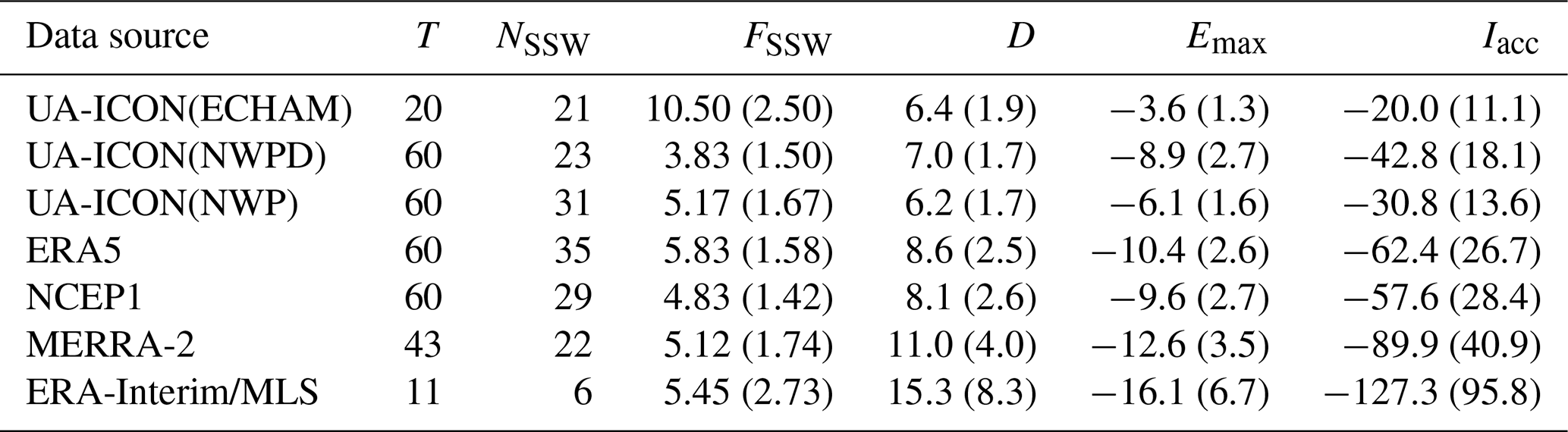
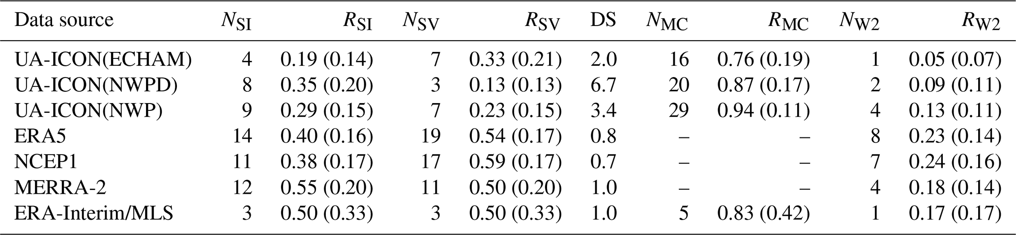
Table 5 Major SSW statistics for data sources (column 1) with numbers and fractions of intense SSWs (N_SI, R_SI in #SI/#SSW), split-vortex SSWs (N_SV, R_SV in #SV/#SSW), and SSW events with mesospheric coupling (N_MC, R_MC in #MC/#SSW) as in Zülicke et al. (2018), the ratio of SSWs with displaced and split polar vortices, and the number and fraction of SSWs with wavenumber-2 preconditioning (N_W2, R_W2 in #W2/#SSW).

The time series of the 10-year moving-average SSW frequencies (Fig. 9a) exhibit large variations for the reanalyses and the UA-ICON(NWP) simulations, whereas the variations for the UA-ICON(ECHAM) simulations are relatively small. The drop to zero for the reanalyses at year 26 corresponds to the 10 years of SSW absence observed from 1988 to 1997, which incidentally is reproduced by UA-ICON(NWPD). Stratospheric variability and the variations in SSW frequency of the observational record have been attributed to several forcing mechanisms: (1) acting from above, such as solar variability (Labitzke, 1987), (2) propagating upward from the troposphere as planetary wave variations related to, e.g., variability of sea surface temperature (SST); El Niño–Southern Oscillation (ENSO) activity (Sassi et al., 2004; Manzini et al., 2006; Domeisen et al., 2019); and variations in the Eurasian snow cover (Cohen et al., 2007; Schimanke et al., 2011), or (3) processes of internal stratospheric variability such as the Quasi-Biennial Oscillation (QBO) (Holton and Tan, 1980). However, none of these external drivers of stratospheric variability is included in the UA-ICON simulations, and the ocean surface state is based on an average over the years 1979–2016. Therefore, the variations in SSW frequency are part of the intrinsic model variability. Other studies, however, emphasize the role of the stratosphere itself in acting as a wave amplifier, as discussed in de la Cámara et al. (2019). The bar charts display the number of SSWs per decade (full colored bars), with the error bars indicating the 95 % confidence interval (CI) (F_SSW in Table 4) derived from a bootstrapping method applied individually to the complete time series of the yearly SSW frequency of each dataset and resampling 50 000 times, with replacement, of the same number of years (the same approach as in Wu and Reichler, 2020). The open yellow bars indicate the average intensity of the SSWs in terms of the averaged accumulated easterly wind anomalies (I_acc in Table 4). The frequency of SSW events during the winter season from November to March (Fig. 9a and F_SSW in Table 4) for the reanalyses is in the range of 4.8 (1.4 CI) to 5.8 (1.6 CI) per decade, given by NCEP/NCAR and ERA5, respectively, whereas MERRA-2 lies in between. Although NCEP/NCAR and ERA5 statistics are derived for the same period, they differ by one event per decade, as some events are not captured by NCEP/NCAR, probably due to the relatively low model top in the stratosphere. MERRA-2 gives a lower frequency of SSWs than ERA5, but this is caused by the shorter period used for MERRA-2, and limiting ERA5 to 1980–2022 shows the same SSW frequency as MERRA-2, whereas for NCEP/NCAR the SSW frequency for 1980–2022 is again lower (4.9 SSWs per decade). There is a decrease in F_SSW and an increase in I_acc when changing from UA-ICON(ECHAM) to UA-ICON(NWP). The high F_SSW in the UA-ICON(ECHAM) simulation is related to the very weak stratospheric polar vortex, leading to frequent transitions to ${\stackrel{\mathrm{‾}}{U}}_{\mathrm{60}\mathrm{N}}$ easterlies and a positive $\stackrel{\mathrm{‾}}{\mathrm{\Delta }T}$ during the winter period (Fig. 6). However, the average I_acc is only low. When applying the NWP physics package, F_SSW and I_acc improve. The UA-ICON(NWP) simulation shows F_SSW in the range of the reanalyses but a lower I_acc than ERA5, NCEP/NCAR, and MERRA-2, which shows the largest I_acc among the reanalyses, whereas the UA-ICON(NWPD) simulation shows a slightly smaller F_SSW but a larger I_acc.

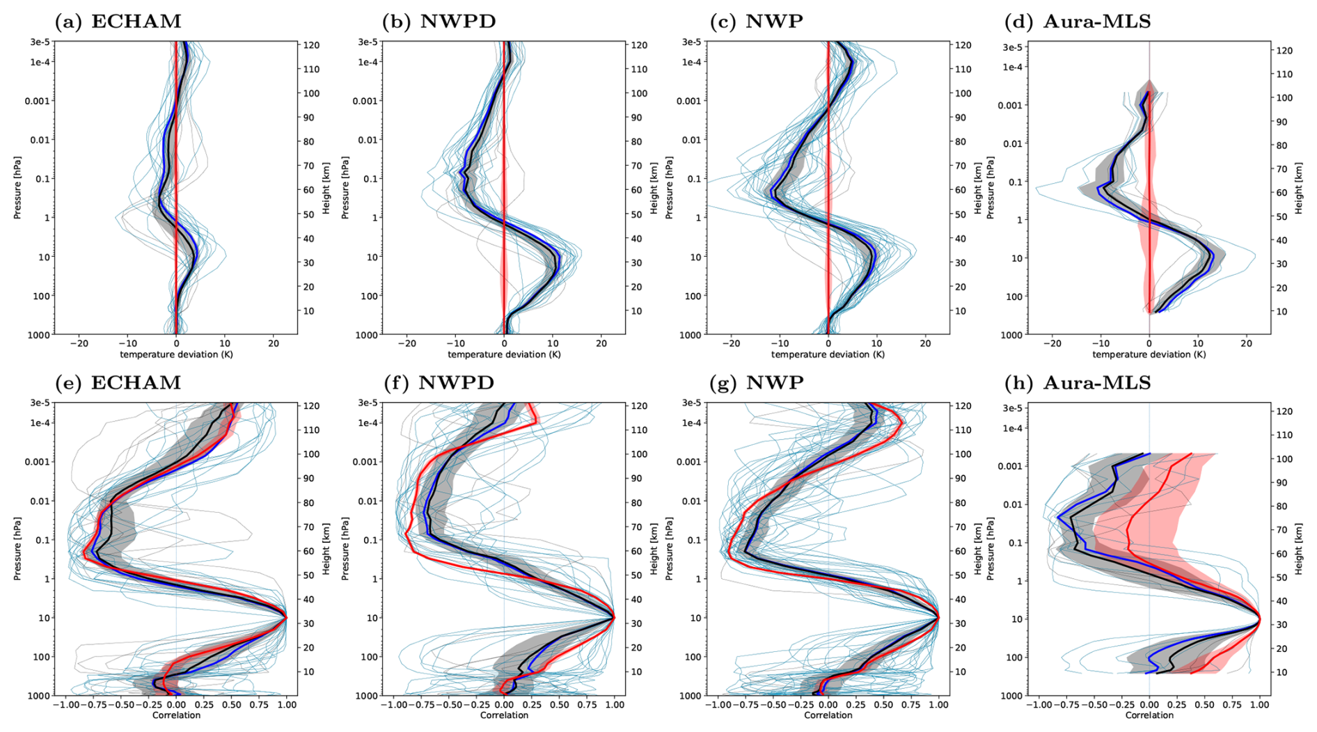
Figure 10 (a–d) Vertical profiles of polar cap temperature anomalies ($\mathrm{\Delta }{\stackrel{\mathrm{‾}}{T}}_{\text{60–90N}}$) in 21 d windows centered at day 0 of SSWs (black and blue) or for the NH winter season from 1 November to 31 March (red) (a–e). (e–h) Vertical profiles of correlations of $\mathrm{\Delta }{\stackrel{\mathrm{‾}}{T}}_{\text{60–90N}}$ in periods as above at different pressure levels with $\mathrm{\Delta }{\stackrel{\mathrm{‾}}{T}}_{\text{60–90N}}$ in the same period at 10 hPa (f–j). The profiles of the individual SSWs are displayed with thin blue or black lines. The thick blue profile is the average of the individual SSW profiles with mesospheric coupling. The thick black line represents the average over all of the SSWs. The thick red profile represents the average of the profiles for the complete winter season. The shaded regions give the 95 % confidence intervals, estimated with a bootstrapping method. The temperature anomalies are relative to the daily long-term mean. The UA-ICON simulations are with (a, f) ECHAM physics, (b, g) the default NWP physics, (c, h) NWP physics and the tuned GWD, (d, i) NWP physics and NWGD tuning, and (e, j) Aura-MLS.

The monthly distribution of the SSW frequency (Fig. 9b) from November to March shows the highest frequency in January for all of the reanalyses, followed by February, December, March, and November. UA-ICON(ECHAM) (black bar) has equally high SSW frequencies in December and January and peaks in February. The UA-ICON(NWPD) simulation (grey bar), applying the default GWD parameters, has an acceptable monthly distribution of SSW frequencies with a maximum in February, but its frequencies are too low in mid-winter and too high in March. After optimizing the GWD parameter in the UA-ICON(NWP) simulation (blue bar), the event frequency is too high in December, November, and March and too low in January and February. The averaged SSW intensity (I_acc) of UA-ICON(NWP) is only comparable to the reanalyses in December and is underestimated in mid-winter and overestimated in November and March.

The UA-ICON(NWP) simulation also shows lower values, compared to the reanalyses, for other wind-based statistics like the event duration (D), the maximum easterly wind (E_max), I_acc (Table 4), and the fraction of intense SSW events with I_acc values exceeding 100 m s⁻¹ (R_SI, Table 5). Regarding these statistics, the UA-ICON(NWPD) simulation with the default GWD setting agrees better with the reanalyses. The necessary tuning of the OGWD harms this aspect of the NH stratospheric winter variability. The SSW duration and the maximum and accumulated easterlies of UA-ICON(NWP) are consistently lower than those of the reanalyses.

Table 5 summarizes additional statistical evaluations of SSW events, focusing on polar vortex geometry, SSW preconditioning, and coupling with the mesosphere. In addition to R_SI, these are the number and fraction of split-vortex SSW events (N_SV and R_SV), the number and fraction of SSWs with mesospheric coupling (N_MC and R_MC), and the number and fraction of SSWs with zonal wavenumber-2 (W2) preconditioning (N_W2 and R_W2). The classification of the polar vortex geometry is based on the method of Charlton and Polvani (2007), applying an elliptic vortex diagnostic in 21 d around day 0. For this purpose, one ellipse is fitted to the pressure field if there is one low-pressure system or two ellipses if there are two low-pressure systems. Thereby, displaced (DV) and split (SV) polar vortices are distinguished. The detection of the SSWs with mesospheric coupling is based on polar cap (60–90°N) area-weighted averaged temperature anomalies ($\mathrm{\Delta }{\stackrel{\mathrm{‾}}{T}}_{\text{60–90N}}$) at 10 and 0.01 hPa. If the 10 hPa stratospheric warming and the mesospheric cooling both exceed 1 standard deviation, the SSW is a mesospheric coupling event. The criterion for W2 preconditioning is based on the method of Bancalá et al. (2012) and requires the amplitude of the 50 hPa geopotential height W2 to be larger than the respective W1 by more than 100 m and the 100 hPa W2 heat flux to be larger than the respective W1 heat flux by more than 15 K m s⁻¹ in the 10 d before the SSW around the day with the largest 10 hPa ${\stackrel{\mathrm{‾}}{U}}_{\mathrm{60}\mathrm{N}}$ deceleration.

We start by comparing R_SV in UA-ICON simulations to reanalyses and an analysis of CMIP6 models by Hall et al. (2021), who used, instead of R_SV, the ratio of SSWs with displaced and split polar vortices (DS). To better compare our measurement to the published DS, we give the DS values in Table 5 and in parentheses in the text. Using the reanalyses as an observational basis, the observed relative number of split-vortex events (R_SV) is in the range 50 %–59 % (1.0–0.7), with differences to a certain degree due to the reanalysis period. All the UA-ICON simulations have a lower R_SV, where UA-ICON(ECHAM), with 33 % (2.0), shows the highest R_SV, the UA-ICON(NWPD) simulation shows the lowest with 13 % (6.7) and 14 %–16 % (6.0–5.2), and the GWD-tuned UA-ICON(NWP) shows an increase to 23 % (3.4). Hall et al. (2021) analyzed the representation of stratospheric polar vortex variability and SSWs in CMIP6 models in comparison to ERA5 and ERA-Interim and found for ERA5 (1979–2020) a displaced- to split-vortex ratio (DS) of 1.5. The ERA5 DS from our vortex geometry analysis is 0.8 (R_SV of 54 %), indicating the detection of more split-vortex SSW events with our algorithm. The multimodel mean DS of the CMIP6 models analyzed in Hall et al. (2021) is 2.2, but the DS range is large, from 0.9 to 9.0. The DS values of the UA-ICON simulations are in the range of the CMIP6 models, with 2.0 for UA-ICON(ECHAM), 6.7 for UA-ICON(NWPD), and 3.4 for UA-ICON(NWP). The deficit of UA-ICON(NWP) in the proper simulation of planetary zonal wavenumber 2 also shows the statistics of W2 preconditioning, which give R_W2 values in the range of only 9 %–13 %, where reanalyses show a W2 preconditioning in 24 % (NCEP1) or 23 % (ERA5) of the SSWs.

As discussed for the averaged SSW-related quantities of UA-ICON(NWP) in Fig. 8, the intense warming of the polar cap stratosphere during SSWs is the result of anomalous wave forcing, leading to adiabatic stratospheric warming, adiabatic cooling in the mesosphere, and adiabatic warming in the thermosphere. Figure 10 shows this stratosphere–mesosphere coupling with profiles of the area-weighted averaged polar cap $\mathrm{\Delta }{\stackrel{\mathrm{‾}}{T}}_{\text{60–90N}}$ anomalies for a time average over 21 d centered at the onset of individual SSWs (thin dashed lines, blue SSWs with MC, and black SSWs without MC). The thick lines represent the averages over the individual SSWs in blue for SSWs with MC and in black for SSWs without MC. The red profiles represent the polar cap $\mathrm{\Delta }{\stackrel{\mathrm{‾}}{T}}_{\text{60–90N}}$ anomalies for a time average over the NH winter period from November 1 to 31 March, including all years. The shaded region around the red and blue averaged profiles represents the 95 % confidence interval from a bootstrapping method. The top row of Fig. 10a–e shows the anomalies of the respective profiles in the long-term daily climatology, with both UA-ICON(NWP) simulations during SSWs showing more intense warm stratospheric anomalies and more intense mesospheric cold anomalies than UA-ICON(ECHAM). The average intensity of the positive stratospheric $\mathrm{\Delta }{\stackrel{\mathrm{‾}}{T}}_{\text{60–90N}}$ in UA-ICON(NWP) (∼ 9 K) is slightly lower than that of Aura-MLS (∼ 11 K). The Aura-MLS stratospheric and mesospheric $\mathrm{\Delta }{\stackrel{\mathrm{‾}}{T}}_{\text{60–90N}}$ is slightly more intense for the average over MC SSWs (blue profile), which is reproduced by the UA-ICON simulation. The magnitude of mesospheric cooling associated with SSWs is represented well in the GWD-tuned UA-ICON(NWP) simulation and compares well with Aura-MLS. The bottom row of Fig. 10f–j shows the correlation of the respective ${\stackrel{\mathrm{‾}}{T}}_{\text{60–90N}}$ values at a pressure level of 10 hPa with all other pressure levels of the UA-ICON simulations and Aura-MLS. Throughout the NH winter period (red profile), the stratosphere is coupled well to the mesosphere, as indicated by the typical anticorrelation between the stratosphere and mesosphere. The average profile of the UA-ICON(NWPD) simulation shows the maximum anticorrelation (∼ −0.75) during SSWs over a more extended altitude region (∼ 70–95 km) compared to UA-ICON(ECHAM) and UA-ICON(NWP), with the largest anticorrelation focused more vertically near ∼ 75 km. By tuning the GWD parameterizations in UA-ICON(NWP), the average profile based on the entire period (thick red), in general, shows similar behavior to the mesospheric anticorrelation focused at a lower altitude. While the vertical structure of the SSW-related anomalies in the middle atmosphere is simulated well, we find that the frequency of mesospheric coupling (diagnosed with R_MC in Table 5) is slightly too high when comparing UA-ICON(NWP) with ERA-Interim/MLS. However, it is well within the uncertainties of the respective datasets and thus is no cause for concern.

6 Tidal analyses

Figure 11 presents the amplitude of the migrating diurnal (upper eight panels) and semidiurnal (lower eight panels) tides in temperature derived from UA-ICON(NWP) and SABER as a function of latitude (50° S–50° N) and height (70–110 km). The retrieval of tides uses the least-squares technique described in Yamazaki and Siddiqui (2024). The SABER tidal climatologies are based on temperature measurements during 22 years (2002–2023), while the UA-ICON(NWP) results are based on hourly temperature outputs of 60 years. It is noted that the tidal analysis of SABER data involves a 60 d window, which might lead to an underestimation of tidal amplitudes.

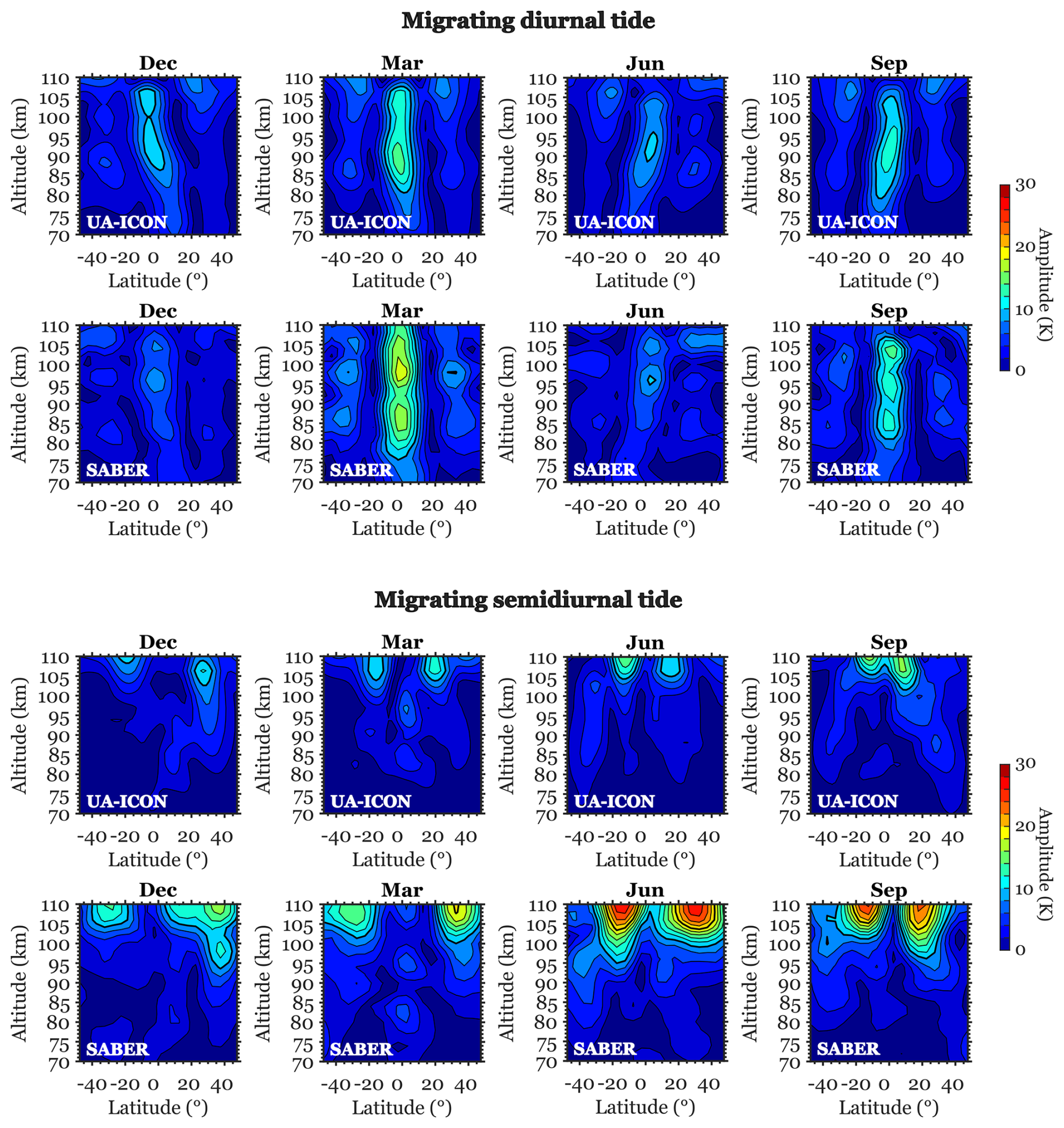
Figure 11 Amplitude of the migrating diurnal and semidiurnal tides in temperature as derived from UA-ICON(NWP) and SABER.

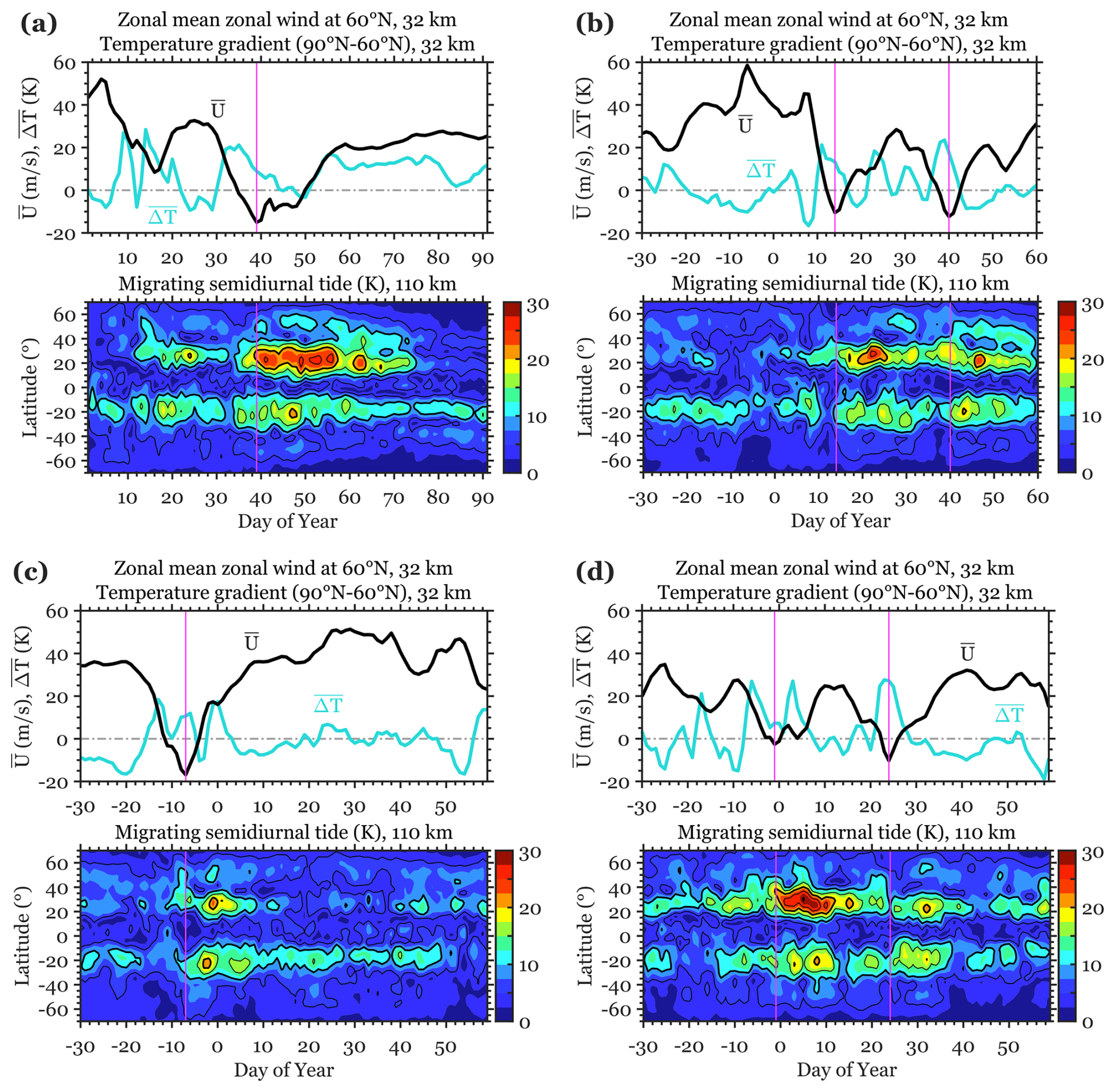
Figure 12 Amplitude of the migrating semidiurnal tide in temperature at 110 km as derived from UA-ICON(NWP) during four selected boreal winters containing major SSWs. The vertical lines correspond to the days of the peak reversal of the zonal mean zonal wind.

The latitude–altitude structure and seasonal variation of the migrating diurnal tide are reproduced well by UA-ICON(NWP). The latitude structure with the maximum temperature perturbation at the Equator and secondary peaks at ±30° corresponds to the (1,1) Hough mode of classical tidal theory (Forbes, 1995). UA-ICON(NWP) also captures the semiannual variation in the amplitude of the migrating diurnal tide. That is, the amplitude is greater during the equinoxes than during the solstices. The semiannual variation of the diurnal tide is well known (Burrage et al., 1995) and is generally attributed to the change in the background atmosphere, which affects the vertical propagation of the tide (McLandress, 2002a, b).

Compared to the migrating diurnal tide, the migrating semidiurnal tide has a longer vertical wavelength and thus can propagate deeper into the thermosphere (Forbes, 1995). UA-ICON(NWP) reproduces a rapid increase in the semidiurnal tidal amplitude above ∼ 95 km. The model also reproduces the seasonal variation with larger amplitudes during June and September than during December and March. However, the model tends to underestimate the amplitude in all seasons. The migrating diurnal and semidiurnal tides in the MLT region from UA-ICON(NWP) also compare well with those from other numerical models such as WACCM-X (e.g., Liu et al., 2018a) and eCMAM (e.g., Beagley et al., 2000). Like UA-ICON(NWP), both these models produce a realistic seasonal variability of migrating tides in the MLT region. However, tidal amplitudes are slightly overestimated in eCMAM (e.g., Gan et al., 2014) and underestimated in WACCM-X (e.g., Liu et al., 2018b) when compared to SABER temperature observations. Tides from UA-ICON(NWP) do not differ significantly from eCMAM and WACCM-X, implying that UA-ICON(NWP) is at least as capable as both of these models of producing migrating tidal variability in the MLT region close to the observations.

We also examine the tidal variability during SSWs as simulated by UA-ICON(NWP). It is well known that tides at MLT altitudes can be significantly altered during SSWs (e.g., Pedatella et al., 2014; Siddiqui et al., 2022). In particular, an enhancement of the migrating semidiurnal tide is a robust feature that has been reported for different SSWs (e.g., Jin et al., 2012; Maute et al., 2015; Siddiqui et al., 2021). Figure 12 presents examples of the migrating semidiurnal tide response to major SSWs over four boreal winters in UA-ICON(NWP). In each winter case, the top panel depicts the zonal mean zonal wind at 60° N and 10 hPa ($\stackrel{\mathrm{‾}}{U}$), along with the difference in temperature between the North Pole and the zonal average at 60° N and 10 hPa ($\stackrel{\mathrm{‾}}{\mathrm{\Delta }T}$). Reversal of the zonal mean zonal wind, accompanied by a reversal of the meridional temperature gradient, signifies the occurrence of a major SSW. The bottom panel shows the amplitude of the migrating semidiurnal tide in temperature at 110 km derived using the method described in Yamazaki (2023). In all of these cases, the enhancement in the tidal amplitude is observed following the peak reversal of the zonal mean zonal wind, consistent with earlier studies. The tidal response is similar during other boreal winters that contain major SSWs, which are not presented here. These results suggest that UA-ICON(NWP) may be well suited to studying the coupling between SSWs and the variability in the middle and upper atmosphere.

7 Discussion, summary, and conclusions

This work introduces a tuned version of the upper-atmospheric extension of the ICON model with the NWP physics package (UA-ICON(NWP)). It represents the mean state and the variability of the MLT reasonably well. Here, we document the parameter optimization for the Warner and McIntyre (1996) (WM96) gravity wave parameterization for the non-orographic gravity waves in UA-ICON and the Lott and Miller (1997) (LM97) parameterization for the orographic gravity waves in UA-ICON, using the NWP physics package to obtain the presented results. With this aim, we apply UA-ICON(NWP) at a horizontal resolution of R2B4 (∼ 160 km) and 120 layers up to an altitude of 150 km. Using a series of perpetual January simulations, we demonstrate the effects of changing the tunable parameters of both the orographic and non-orographic gravity wave parameterizations. Based on these simulations, we choose one parameter setup to best perform for the middle and upper atmosphere in terms of the climatology in the MLT and the variability during the Northern Hemisphere winter season. We recommend, for the non-orographic WM96 parameterization, increasing a dimensionless factor of the saturation momentum flux density spectrum and decreasing the total launch momentum flux and, in the LM97 parameterization, adapting the low-level wake drag constant, the gravity wave drag constant, and the critical Froude number, as detailed in Table 3. With these settings, UA-ICON(NWP) has a sufficiently strong upper-mesospheric eastward-directed zonal wind tendency (up to 140 m s⁻¹ d⁻¹) to drive a mean meridional residual circulation strong enough to create the required adiabatic cooling of the summer mesopause region. The climatological seasonal averages of the polar summer mesopause temperatures of UA-ICON(NWP) are as low as shown by SABER in the austral summer (< 150 K) and boreal summer (< 140 K). However, the altitude and vertical extent of these low summer mesopause temperatures are slightly too low and too narrow in UA-ICON(NWP).

Introducing a stronger NGWD into UA-ICON(NWP) partly reverses the direction or decelerates the magnitude of the zonal mean zonal wind in the lower thermosphere from the prevailing eastward-directed flow in the stratosphere and mesosphere during the winter seasons to a westward-directed flow or a weak eastward-directed flow in the MLT. The magnitudes of these zonal wind changes in UA-ICON(NWP) agree well with the URAP zonal mean zonal wind changes in these seasons. The vertical extent of the mesospheric polar vortex in UA-ICON(NWP), however, is limited to ∼ 80 km, which is common behavior of GCMs or CCMs with extension to the lower thermosphere, running at a coarse horizontal resolution and thereby relying on the parameterization of the NGWD, e.g., HAMMONIA (Schmidt et al., 2006), WACCM6 (Gettelman et al., 2019), or UA-ICON (version ua-icon-1.0) (Borchert et al., 2019). Increasing the horizontal resolution allows GCMs to resolve at least a fraction of the NGWD down to the mesoscale and at a sufficient horizontal resolution, and they do not require GW parameterizations (e.g., Liu et al., 2014; Becker and Vadas, 2018, 2020; Stephan et al., 2020). The KMCM (Becker and Vadas, 2018) and HIAMCM (Becker and Vadas, 2020), spectral models both with a truncation of 240, 190 layers up to $\mathrm{1.5}\times {\mathrm{10}}^{-\mathrm{5}}$ hPa (KMCM), and 260 layers up to $\mathrm{6}\times {\mathrm{10}}^{-\mathrm{9}}$ hPa (HIAMCM) in the thermosphere, resolve horizontal wavelengths with λ∼ 165 km and do not parameterize any GWs. Becker and Vadas (2020) discussed the height of the MLT summer zonal wind reversal in HIAMCM, which simulates GWs explicitly, and compared it to CIRA86, stating that the zonal wind reversal from westward to eastward flow is too high in altitude, which is a consequence of the eastward GWD being too high by about 10 km. This contrasts with the coarser models relying on GW parameterizations, where the wind reversal is too low in altitude. While both types of models, GW-resolving and GW-parameterizing, have problems modeling the summer MLT wind reversal correctly, Becker and Vadas (2020) stated that, on average, GW-resolving GCMs do not simulate the MLT eastward–westward reversal in winter, which is at least in better agreement with climatologies derived for local radar observations. Smith (2012) discussed the discrepancies between zonal mean zonal wind climatologies derived from satellite data and localized radar observations and explained the deviations with planetary-scale variations which cause persistent longitudinal variations in the zonal wind. Hindley et al. (2022) showed the difference in meteor-radar-derived zonal wind over South Georgia (54° S, 30° W) and in WACCM6. Both show the wind reversal from westward to eastward zonal winds in summer. However, they differ in winter, with the meteor radar showing an eastward zonal wind throughout the MLT as an extension of the polar vortex into the upper mesosphere, whereas WACCM6 shows the transition from eastward to westward zonal winds. UA-ICON(NWP) behaves similarly to WACCM6, which is typical for models with parameterized GWs. Using UA-ICON (version ua-icon-1.0 with ECHAM physics) in a high-resolution configuration (R2B7; ∼ 20 km horizontally, 180 layers) without any parameterized GWD, Stephan et al. (2020) showed that the model sufficiently generates resolved GW momentum flux in the MLT region to model realistic thermal and dynamic structures. Still, using wave-resolving UA-ICON versions remains a computational challenge for future model applications. At present, we recommend our tuned low-resolution version for efficient simulation of the MLT region for long simulations or ensembles.

The mesospheric MMC, driven by the dissipation of GWs, connects the summer MLT region with the respective lower-mesospheric and lower-stratospheric winter atmospheres, which results in a descending motion at the high latitudes and adiabatic warming of the stratopause regions. When increasing the parameterized GWD in UA-ICON(NWP), the MMC intensifies, with the consequence that the winter mesopause temperatures rise, creating a warm bias compared to the SABER observations. This is a drawback for the proper simulation of the summer MLT temperatures. It remains to be investigated whether transient and horizontal GW propagation allowing non-orographic gravity wave parameterizations (e.g., Bölöni et al., 2021) could resolve the current numerical dilemma. While our tuning attempt for the NGWD focused on changing the saturation conditions for NGWs and the source strength, by varying parameters without latitudinal variation, Richter et al. (2010) tuned the NGWD in WACCM3 by introducing a source-oriented GW parameterization, accounting for variability in convective activity and frontal systems. One detail of their tuning success is the SH springtime transition of the zonal wind, which shifts to an earlier date. The transition to an easterly flow at 60° S at 10 hPa occurs in early November for ERA5 data, which the UA-ICON(ECHAM) simulation matches perfectly. The UA-ICON(NWP) simulations show the transition in late November, which is only slightly shifted to a later date by the GWD tuning (Fig. S4 in the Supplement) compared with the WACCM experiments shown in Fig. 10 of Richter et al. (2010), which appear at the end of December.

A relevant benchmark test for GCMs and CCMs extending to the mesosphere or lower thermosphere is their ability to model major SSWs with a realistic frequency and strength, including the related upward coupling with the mesosphere. Compared to the initial version of UA-ICON, based mostly on the ECHAM physics package (Borchert et al., 2019), the version presented in this work, based on the NWP physics package, has a significantly better representation of the stratospheric and mesospheric Northern Hemisphere winter polar vortex and its variability. Our statistical evaluation of SSWs includes a mesospheric coupling diagnostic (Zülicke et al., 2018), a geometric vortex diagnostic distinguishing splits from displaced vortex SSWs (Charlton and Polvani, 2007), and a wave preconditioning diagnostic (Bancalá et al., 2012). The overall frequency of 5.2 SSWs per decade is well within the range of 4.8–5.8 SSWs per decade estimated by the reanalysis products. However, their intensity as quantified with the accumulated easterlies (I_acc) was found to be −31 m s⁻¹, less than the range of the observed −58 to −90 m s⁻¹. Mesospheric and stratospheric temperatures are usually anticorrelated, and this structure is simulated well with UA-ICON(NWP). Although the SSW events with a strong mesospheric response are slightly too frequent, the close coupling of the mesosphere with the stratosphere is included. Hence, in a statistical sense, the model's performance in the stratosphere is essential for the model's performance in the mesosphere.

The tidal analyses showed the amplitude of the migrating diurnal and semidiurnal tides in temperature to be represented well in UA-ICON(NWP), with the latitudinal structure and the seasonal variability in an acceptable state compared to the SABER-derived tides. The enhancement of the migrating semidiurnal tide during major SSWs is reproduced well in UA-ICON(NWP), indicating a good representation of vertical coupling mechanisms in the model.

In conclusion, UA-ICON (version ua-icon-2.1) at a horizontal resolution of ∼ 160 km is a highly performing upper-atmospheric model available for vertical atmospheric coupling studies and investigation of the MLT region. In addition, this paper has pointed out several challenges which need to be tackled in atmospheric modeling with UA-ICON. These are the lack of an ability to tune, equally well, the stratosphere and mesosphere, the equatorward bias of jet positions, the possibly related biases of the polar vortex in SSW strengths and wavenumber-2 preconditioning, the too narrow and low cold summer MLT, or the winter polar vortex not extending high enough. We expect to solve these problems with high-resolution modeling to increase the fraction of the resolved GWD, a method UA-ICON is particularly designed for.