SURFER v3.0: a fast model with ice sheet tipping points and carbon cycle feedbacks for short- and long-term climate scenarios

Simple climate models that are computationally inexpensive, transparent, and easy to modify are useful for assessing climate policies in the presence of uncertainties. This motivated the creation of SURFER v2.0, a model designed to estimate the impact of CO₂ emissions and solar radiation modification on global mean temperatures, sea level rise, and ocean pH. However, SURFER v2.0 is unsuitable for simulations beyond a few thousand years because it lacks some carbon cycle processes. This is problematic for assessing the long-term evolution of the Earth system, particularly the dynamics of ice sheets and the resulting sea level rise. Here, we present SURFER v3.0, an extension to SURFER v2.0 that allows for accurate simulation of the climate, carbon cycle, and sea level rise on timescales ranging from decades to millions of years. We incorporated a dynamic cycling of alkalinity in the ocean, a carbonate sediments reservoir, and weathering fluxes into the model. With these additions, we show that SURFER v3.0 reproduces results from a large class of models, ranging from centennial Coupled Model Intercomparison Project Phase 6 (CMIP6) projections to 1 Myr runs performed with the cGENIE model of intermediate complexity. We show that compared to SURFER v2.0, including long-term carbon cycle processes in SURFER v3.0 leads to a stabilisation of the Greenland ice sheet for the middle of the road emission scenarios and to a significant reduction in the sea level rise contribution from Antarctica for high-emission scenarios.

1 Introduction

Human activities have significantly altered Earth's climate by releasing greenhouse gases, primarily carbon dioxide (CO₂) and methane (CH₄), into the atmosphere at unprecedented rates (IPCC, 2021a). The consequences of these emissions are already palpable, with 2024 marking the warmest year on record (WMO, 2025). Moreover, the frequency and intensity of extreme-weather events such as heatwaves, droughts, and heavy precipitation have increased and are projected to increase further under global warming (IPCC, 2021b). While these impacts are immediate and observable, others unfold over longer time frames. For instance, the melting polar ice caps will contribute to sea level rise for centuries and even millennia after emissions of greenhouse gases are reduced or stopped (Clark et al., 2016; Van Breedam et al., 2020). There is also growing concern over climate tipping points, where potentially abrupt and irreversible changes could occur and lead to cascades of unforeseen consequences in the long-term trajectories of the Earth system (Lenton et al., 2008, 2019; Armstrong McKay et al., 2022; Steffen et al., 2018).

Making informed decisions about climate change thus necessitates a comprehensive examination across multiple temporal scales to balance the immediate needs of current populations with the imperative of safeguarding the planet's habitability for future generations (Raworth, 2012). To this end, climate models are indispensable for scientists and policymakers. They come in different sizes and complexities (see Sect. 3.2 in Goosse, 2015). On one side of the complexity spectrum, state-of-the-art Earth system models include detailed representations of physical and biogeochemical processes. However, due to their size and complexity, they are hard to analyse and are computationally expensive to run, with most simulations ending in 2100 (for example, this is the case in most Coupled Model Intercomparison Phase 6 (CMIP6) experiments). On the other side of the spectrum, conceptual box models trade complexity and spatial resolution for speed and simplicity. They provide valuable insights into fundamental climate processes and feedbacks, facilitating transparent and intuitive assessments of long-term climate trends. Due to their low computational cost, they can be run many times, with different choices of parameters and for different forcing scenarios. This allows an extensive exploration of mitigation and adaptation strategies, such as taking into account possible errors caused by simplifications and other knowledge gaps.

This is the spirit in which SURFER was designed (Martínez Montero et al., 2022). SURFER v2.0 is a model based on nine ordinary differential equations designed to estimate global mean temperature increase, sea level rise and ocean acidification in response to CO₂ emissions and aerosol injections. It is fast and easy to understand and modify, making it appropriate for use in policy assessments. For example, in Montero et al. (2023), it helped assess the long-term sustainability of short-term climate policies based on a novel commitment metric. Yet SURFER v2.0 lacks some processes in its carbon cycle implementation. It can only simulate quantities reliably for up to 2 or 3 millennia and only accounts for carbon dioxide emissions in the carbon cycle. Here, we introduce an extended version of the model with new processes, SURFER v3.0. Among other things, we have added a representation of atmospheric methane, a distinction between land use and fossil emissions, an additional oceanic layer, a dependence of the solubility and dissociation constants on temperature and pressure, a dynamic representation of alkalinity, a sediment box, and weathering processes.

The present paper is structured as follows. We explain in detail the new additions to SURFER v3.0 in Sect. 2. In Sect. 3, we compare the results of SURFER v3.0 to other models on timescales ranging from centuries to a million years. We first show that SURFER v3.0 can reproduce the historical record. Then, we show that SURFER v3.0 is in the range of Intergovernmental Panel on Climate Change (IPCC) class models for different quantities modelled up to 2100 and 2300 CE. We next compare the CO₂ draw-down computed by SURFER over 10 000 years to models that participated in the Long-Tail Model Intercomparison Project (LTMIP). Lastly, we compare SURFER v3.0 outputs to 1 Myr runs performed with the cGENIE climate model of intermediate complexity. In Sect. 4, we show that including new processes in the carbon cycle reduces the committed sea level rise (SLR) estimations on millennial timescales compared to SURFER v2.0. In Sect. 5 we discuss the advantages and limitations of our model. Finally, in Sect. 6, we conclude and provide some perspectives on future research.

2 Model specification

The nine ordinary differential equations of SURFER v2.0 describe the exchanges of carbon between four different reservoirs (atmosphere, upper-ocean layer, deeper-ocean layer, and land), the evolution of temperature anomalies of two different reservoirs (upper-ocean layer and deeper-ocean layer), the volumes of the Greenland and Antarctic ice sheets, and the sea level rise related to glaciers (Martínez Montero et al., 2022). In version v3.0, we have added the following:

• an ocean layer of intermediate depth,

• a sediment box with CaCO₃ accumulation and burial fluxes,

• dynamic alkalinity cycling between the three ocean layers,

• an explicit description of the soft-tissue and carbonate pumps in the ocean,

• volcanic outgassing and weathering fluxes,

• an equation for methane evolution in the atmosphere,

• a temperature and depth (pressure) dependence of the solubility and dissociation constants, and

• a second equation for the land reservoir that allows for a better distinction between land use and fossil greenhouse gas emissions.

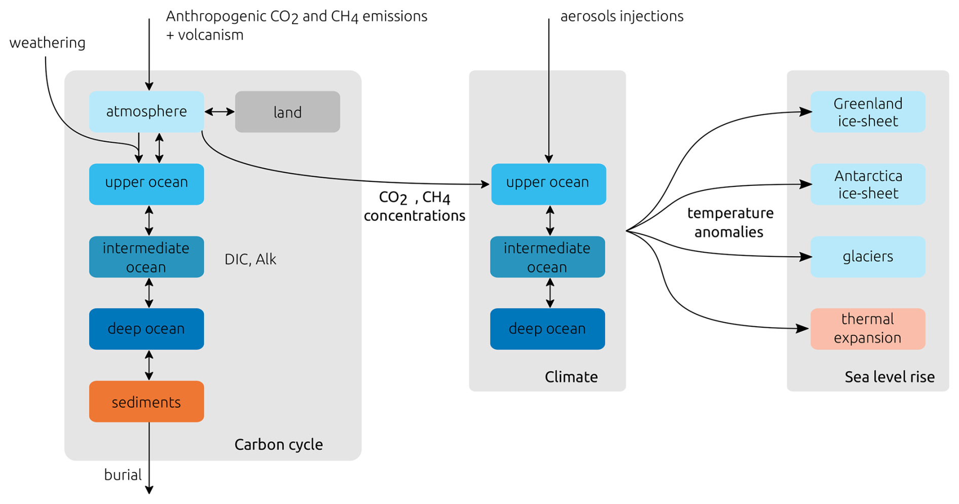
SURFER v3.0 now consists of 17 coupled ordinary differential equations, while keeping its original architecture. It contains three main components for the carbon cycle, the climate, and the sea level. The model is forced by land use and fossil emissions of CO₂ and CH₄ and by aerosol injections. State variables defining the model components, carbon and energy fluxes between those components, and forcings are schematically summarised in Fig. 1.

Figure 1 Conceptual diagram of SURFER v3.0.

In this section, we explain the model implementation in detail. Section 2.1–2.3 focus on the implementation of the carbon, climate, and sea level rise components, respectively. In Sect. 2.4, we show how the model was calibrated and how the initial conditions were chosen. Section 2.5 discusses the algorithmic implementation and speed.

2.1 Carbon cycle component

The equations for the carbon cycle component of SURFER v3.0 are given by

$$\begin{array}{}\text{(1)}& {\displaystyle }\begin{array}{rl}{\displaystyle \frac{\mathrm{d}{M}_{\mathrm{A}}}{\mathrm{d}t}}& =V+E_{\mathrm{fossil}}^{{\mathrm{CO}}_{\mathrm{2}}}+E_{\text{land use}}^{{\mathrm{CO}}_{\mathrm{2}}}-F_{\mathrm{A}\to \mathrm{U}}-F_{\mathrm{A}\to \mathrm{L}}\\ & +F_{{\mathrm{CH}}_{\mathrm{4}},\mathrm{ox}}-E_{\mathrm{natural}}^{{\mathrm{CH}}_{\mathrm{4}}}-F_{\mathrm{weathering}},\end{array}\text{(2)}& {\displaystyle }{\displaystyle \frac{\mathrm{d}{M}_{\mathrm{A}}^{{\mathrm{CH}}_{\mathrm{4}}}}{\mathrm{d}t}}=E_{\mathrm{fossil}}^{{\mathrm{CH}}_{\mathrm{4}}}+E_{\text{land use}}^{{\mathrm{CH}}_{\mathrm{4}}}+E_{\mathrm{natural}}^{{\mathrm{CH}}_{\mathrm{4}}}-F_{{\mathrm{CH}}_{\mathrm{4}},\mathrm{ox}},\text{(3)}& {\displaystyle }{\displaystyle \frac{\mathrm{d}{M}_{\mathrm{L}}}{\mathrm{d}t}}=F_{\mathrm{A}\to \mathrm{L}}-E_{\text{land use}}^{{\mathrm{CO}}_{\mathrm{2}}}-E_{\text{land use}}^{{\mathrm{CH}}_{\mathrm{4}}},\text{(4)}& {\displaystyle }{\displaystyle \frac{\mathrm{d}{M}_{\mathrm{U}}}{\mathrm{d}t}}=F_{\mathrm{A}\to \mathrm{U}}-F_{\mathrm{U}\to \mathrm{I}}+F_{\mathrm{river}},\end{array}$$

$$\begin{array}{}\text{(5)}& {\displaystyle }{\displaystyle \frac{\mathrm{d}{M}_{\mathrm{I}}}{\mathrm{d}t}}=F_{\mathrm{U}\to \mathrm{I}}-F_{\mathrm{I}\to \mathrm{D}},\text{(6)}& {\displaystyle }{\displaystyle \frac{\mathrm{d}{M}_{\mathrm{D}}}{\mathrm{d}t}}=F_{\mathrm{I}\to \mathrm{D}}-F_{\mathrm{acc}},\text{(7)}& {\displaystyle }{\displaystyle \frac{\mathrm{d}{\stackrel{\mathrm{̃}}{Q}}_{\mathrm{U}}}{\mathrm{d}t}}=-{\stackrel{\mathrm{̃}}{F}}_{\mathrm{U}\to \mathrm{I}}+{\stackrel{\mathrm{̃}}{F}}_{\mathrm{river}},\text{(8)}& {\displaystyle }{\displaystyle \frac{\mathrm{d}{\stackrel{\mathrm{̃}}{Q}}_{\mathrm{I}}}{\mathrm{d}t}}={\stackrel{\mathrm{̃}}{F}}_{\mathrm{U}\to \mathrm{I}}-{\stackrel{\mathrm{̃}}{F}}_{\mathrm{I}\to \mathrm{D}},\text{(9)}& {\displaystyle }{\displaystyle \frac{\mathrm{d}{\stackrel{\mathrm{̃}}{Q}}_{\mathrm{D}}}{\mathrm{d}t}}={\stackrel{\mathrm{̃}}{F}}_{\mathrm{I}\to \mathrm{D}}-{\stackrel{\mathrm{̃}}{F}}_{\mathrm{acc}},\text{(10)}& {\displaystyle }{\displaystyle \frac{\mathrm{d}{M}_{\mathrm{S}}}{\mathrm{d}t}}=F_{\mathrm{acc}}-F_{\mathrm{burial}}.\end{array}$$

They describe the fluxes of carbon between six reservoirs: the atmosphere (A); the land (L); the upper- (U), intermediate- (I), and deep-ocean (D) layers; and the deep-sea sediments (S). M_A and $M_{\mathrm{A}}^{{\mathrm{CH}}_{\mathrm{4}}}$ are the masses of carbon in the atmosphere in CO₂ and CH₄ forms, respectively. M_L is the mass of carbon on land (in vegetation and soils), and M_S is the mass of carbon in the erodible CaCO₃ deep-sea sediments. M_U, M_I and M_D are the masses of dissolved inorganic carbon in the ocean layers, while ${\stackrel{\mathrm{̃}}{Q}}_{\mathrm{U}}$, ${\stackrel{\mathrm{̃}}{Q}}_{\mathrm{I}}$, and ${\stackrel{\mathrm{̃}}{Q}}_{\mathrm{D}}$ are total alkalinities. All these quantities are expressed in PgC and the fluxes in PgC yr⁻¹ (Eq. 14 explains what this means for alkalinity).

Variable names are chosen to be self-explanatory, and tildes indicate quantities and fluxes related to alkalinity. Volcanism (V) and anthropogenic CO₂ emissions ($E_{\mathrm{fossil}}^{{\mathrm{CO}}_{\mathrm{2}}}$, $E_{\text{land use}}^{{\mathrm{CO}}_{\mathrm{2}}}$) increase the CO₂ content of the atmosphere. Methane anthropogenic emissions ($E_{\mathrm{fossil}}^{{\mathrm{CH}}_{\mathrm{4}}}$, $E_{\text{land use}}^{{\mathrm{CH}}_{\mathrm{4}}}$) as well as natural emissions ($E_{\mathrm{natural}}^{{\mathrm{CH}}_{\mathrm{4}}}$) increase the CH₄ content in the atmosphere. Methane is rapidly oxidised into CO₂ ($F_{{\mathrm{CH}}_{\mathrm{4}},\mathrm{ox}}$). Atmosphere and land reservoirs exchange CO₂ through photosynthesis and respiration (combined in F_A→L). Weathering (F_weathering) removes carbon dioxide from the atmosphere through chemical reactions with rocks and minerals. The products of these reactions are then transported to the ocean by the rivers (F_river, ${\stackrel{\mathrm{̃}}{F}}_{\mathrm{river}}$). Carbon is exchanged between the different layers of the ocean by mixing and the different carbon pumps (F_U→I, F_I→D, ${\stackrel{\mathrm{̃}}{F}}_{\mathrm{U}\to \mathrm{I}}$, ${\stackrel{\mathrm{̃}}{F}}_{\mathrm{I}\to \mathrm{D}}$). A fraction of the carbon accumulates as sediments on the ocean floor (F_acc, ${\stackrel{\mathrm{̃}}{F}}_{\mathrm{acc}}$) where it can be permanently buried (F_burial) and removed from the system. Ultimately, movements in plate tectonics transport this carbon to the mantle of the Earth (not explicitly modelled in SURFER) where it will be transformed back to CO₂ and eventually emitted in the atmosphere through volcanism, closing the cycle (for a detailed description of the full carbon cycle, see e.g. Archer, 2010)

We detail the implementation of the above fluxes in Sect. 2.1.4 to 2.1.9. Before that, we motivate the addition of a new oceanic layer (Sect. 2.1.1) and discuss the treatment of alkalinity (Sect. 2.1.2) and of the solubility and dissociation constants (Sect. 2.1.3).

2.1.1 Additional ocean layer

SURFER v2.0 used two ocean layers: an upper layer (U) of 150 m in depth and a deep layer (D) of 3000 m in depth. In SURFER v3.0 we use three ocean layers: an upper layer (U) of 150 m in depth, an intermediate layer (I) of 500 m in depth, and a deep layer (D) of 3150 m in depth. Overall, the total ocean depth in SURFER v3.0 is greater than in SURFER v2.0 and closer to the global mean estimate (∼3700 m). The new intermediate layer allows a smoother transition between the upper and deeper layers, which have different properties (temperature, salinity, pH, etc.); see Fig. 3. It also allows faster carbon transport out of the upper layer because the exchange with the new intermediate layer is faster than with the old, deep layer. This modification partly fixes two problems that we had in SURFER v2.0 and that are visible in Fig. 7: CO₂ uptake by the ocean was too slow, and the surface pH decreased too quickly (the surface ocean acidified too quickly; see Martínez Montero et al., 2022). Indeed, since the dissolved CO₂ now leaves the upper layer more quickly, the surface ocean can absorb CO₂ from the atmosphere at faster rates. Moreover, with reduced “stagnation” of dissolved CO₂ in the upper layer, surface acidity increases more slowly (pH decreases more slowly). Differences in atmosphere-to-ocean carbon flux and surface ocean pH between SURFER v2.0 and SURFER v3.0 are shown in Fig. 7.

2.1.2 Total alkalinity

Dissolved inorganic carbon (DIC) is defined as the sum of the following carbonate species: carbonate ions, CO${}_{\mathrm{3}}^{\mathrm{2}-}$; bicarbonate ions, HCO${}_{\mathrm{3}}^{-}$; and H₂CO${}_{\mathrm{3}}^{*}$, which represents a mix of aqueous carbon dioxide CO₂(aqueous) and carbonic acid H₂CO₃. For concentrations, we have

$$\begin{array}{}\text{(11)}& \mathrm{DIC}=\left[{{\mathrm{H}}_{\mathrm{2}}{\mathrm{CO}}_{\mathrm{3}}}^{*}\right]+\left[{\mathrm{HCO}}_{\mathrm{3}}^{-}\right]+\left[{\mathrm{CO}}_{\mathrm{3}}^{\mathrm{2}-}\right].\end{array}$$

Alkalinity, on the other hand, is defined as the excess of bases over acids in water (Middelburg et al., 2020):

$$\begin{array}{}\text{(12)}& \begin{array}{rl}\mathrm{Alk}& =\left[{\mathrm{HCO}}_{\mathrm{3}}^{-}\right]+\mathrm{2}\left[{\mathrm{CO}}_{\mathrm{3}}^{\mathrm{2}-}\right]+\left[{\mathrm{OH}}^{-}\right]-\left[{\mathrm{H}}^{+}\right]\\ & +\left[\mathrm{B}(\mathrm{OH}{)}_{\mathrm{4}}^{-}\right]+\mathrm{minor}\mathrm{bases}.\end{array}\end{array}$$

Intuitively, it measures the ability of a water mass to resist changes in pH when an acid is added. This happens, for example, when excess CO₂ in the atmosphere dissolves in seawater (see Reactions R1–R3). Alkalinity thus plays a crucial role in buffering ocean acidification, which is important for many marine organisms that depend on stable pH levels for their survival and growth (Ross et al., 2011). Being related to the concentrations of dissolved inorganic carbon species (CO${}_{\mathrm{3}}^{\mathrm{2}-}$ and HCO${}_{\mathrm{3}}^{-}$), alkalinity also has a role in regulating the oceanic uptake of atmospheric CO₂. In SURFER v2.0, alkalinity is considered constant and is furthermore approximated by carbonate alkalinity: $\mathrm{Alk}\approx {\mathrm{Alk}}_{\mathrm{C}}=\left[{\mathrm{HCO}}_{\mathrm{3}}^{-}\right]+\mathrm{2}\left[{\mathrm{CO}}_{\mathrm{3}}^{\mathrm{2}-}\right]$. In SURFER v3.0, we include CaCO₃ sediment dissolution, and this requires having variable alkalinity (Eqs. 7–9). We estimate alkalinity based on the carbonate, borate, and water self-ionisation alkalinity (CBW), which includes the contributions of the hydroxide ions [OH⁻], free protons [H⁺], and borate ions [B(OH)${}_{\mathrm{4}}^{-}$]:

$$\begin{array}{}\text{(13)}& \begin{array}{rl}\mathrm{Alk}& \approx {\mathrm{Alk}}_{\mathrm{CBW}}=\left[{\mathrm{HCO}}_{\mathrm{3}}^{-}\right]+\mathrm{2}\left[{\mathrm{CO}}_{\mathrm{3}}^{\mathrm{2}-}\right]+\left[{\mathrm{OH}}^{-}\right]\\ & -\left[{\mathrm{H}}^{+}\right]+\left[\mathrm{B}(\mathrm{OH}{)}_{\mathrm{4}}^{-}\right].\end{array}\end{array}$$

This treatment produces more accurate computations of the concentration of chemical species than SURFER v2.0, specifically [H⁺] and thus pH, but comes at a greater computational cost; see Appendix C for more details. It is also important to note that despite these improvements, our treatment still omits certain chemical species that may become relevant under specific conditions. For instance, the contributions of H₂S and HS⁻ to alkalinity are non-negligible in anoxic or euxinic environments (Xu et al., 2017).

We use units of PgC for the variables representing alkalinity ${\stackrel{\mathrm{̃}}{Q}}_{\mathrm{U}}$, ${\stackrel{\mathrm{̃}}{Q}}_{\mathrm{I}}$, and ${\stackrel{\mathrm{̃}}{Q}}_{\mathrm{D}}$ even though our working approximation now includes terms that do not contain carbon. We do this for purely practical reasons, as all other variables of the carbon cycle component are also in PgC. The alkalinity concentration Alk_i for the layer $i\in \mathit{\{}\mathrm{U},\mathrm{I},\mathrm{D}\mathit{\}}$ in µmol kg⁻¹, a more common unit, is simply given by

$$\begin{array}{}\text{(14)}& {\mathrm{Alk}}_i={\displaystyle \frac{{\stackrel{\mathrm{̃}}{Q}}_i}{W_i{\stackrel{\mathrm{‾}}{m}}_{\mathrm{C}}}}\times {\mathrm{10}}^{\mathrm{18}},\end{array}$$

where W_i is the weight in kilograms of the ocean layer i, and ${\stackrel{\mathrm{‾}}{m}}_{\mathrm{C}}$ is the molar mass of carbon in mol kg⁻¹. This is the same equation as that for the conversion from dissolved inorganic carbon mass in PgC to concentrations in µmol kg⁻¹:

$$\begin{array}{}\text{(15)}& {\mathrm{DIC}}_i={\displaystyle \frac{M_i}{W_i{\stackrel{\mathrm{‾}}{m}}_{\mathrm{C}}}}\times {\mathrm{10}}^{\mathrm{18}}.\end{array}$$

The weight of layer i is given by

$$\begin{array}{}\text{(16)}& W_i={\displaystyle \frac{h_i{\stackrel{\mathrm{‾}}{m}}_{\mathrm{w}}{m}_{\mathrm{O}}}{h_{\mathrm{U}}+h_{\mathrm{I}}+h_{\mathrm{D}}}},\end{array}$$

with ${\stackrel{\mathrm{‾}}{m}}_{\mathrm{w}}$ the molar mass of water and m_O the number of moles in the ocean.

2.1.3 Solubility and dissociation constants

When atmospheric CO₂ enters the ocean, it undergoes a series of chemical reactions:

$$\begin{array}{}\text{(R1)}& {\displaystyle }& {\displaystyle }{\mathrm{CO}}_{\mathrm{2}}\left(\mathrm{gas}\right)+{\mathrm{H}}_{\mathrm{2}}\mathrm{O}\rightleftharpoons {{\mathrm{H}}_{\mathrm{2}}{\mathrm{CO}}_{\mathrm{3}}}^{*},\text{(R2)}& {\displaystyle }& {\displaystyle }{{\mathrm{H}}_{\mathrm{2}}{\mathrm{CO}}_{\mathrm{3}}}^{*}\rightleftharpoons {\mathrm{HCO}}_{\mathrm{3}}^{-}+{\mathrm{H}}^{+},\text{(R3)}& {\displaystyle }& {\displaystyle }{\mathrm{HCO}}_{\mathrm{3}}^{-}\rightleftharpoons {\mathrm{CO}}_{\mathrm{3}}^{\mathrm{2}-}+\mathrm{2}{\mathrm{H}}^{+}.\end{array}$$

These reactions are fast, and we assume that they are in equilibrium (Sarmiento and Gruber, 2006). The relationships between the equilibrium concentrations of the different chemical species are determined by the dissociation constants:

$$\begin{array}{}\text{(17)}& {\displaystyle }& {\displaystyle }{K}_{\mathrm{1}}={\displaystyle \frac{\left[{\mathrm{H}}^{+}\right]\left[{\mathrm{HCO}}_{\mathrm{3}}^{-}\right]}{\left[{{\mathrm{H}}_{\mathrm{2}}{\mathrm{CO}}_{\mathrm{3}}}^{*}\right]}},\text{(18)}& {\displaystyle }& {\displaystyle }{K}_{\mathrm{2}}={\displaystyle \frac{\left[{\mathrm{H}}^{+}\right]\left[{\mathrm{CO}}_{\mathrm{3}}^{\mathrm{2}-}\right]}{\left[{\mathrm{HCO}}_{\mathrm{3}}^{-}\right]}}.\end{array}$$

Similarly, we have for the equilibrium concentrations of OH⁻ and B(OH)${}_{\mathrm{4}}^{-}$

$$\begin{array}{}\text{(19)}& {\displaystyle }& {\displaystyle }{K}_{\mathrm{w}}=\left[{\mathrm{H}}^{+}\right]\left[{\mathrm{OH}}^{-}\right],\text{(20)}& {\displaystyle }& {\displaystyle }{K}_{\mathrm{b}}={\displaystyle \frac{\left[{\mathrm{H}}^{+}\right]\left[\mathrm{B}(\mathrm{OH}{)}_{\mathrm{4}}^{-}\right]}{\left[{\mathrm{H}}_{\mathrm{3}}{\mathrm{BO}}_{\mathrm{3}}\right]}},\end{array}$$

where we additionally assume that the total equilibrium boron concentration is proportional to salinity (Uppström, 1974):

$$\begin{array}{}\text{(21)}& \mathrm{TB}=\left[\mathrm{B}(\mathrm{OH}{)}_{\mathrm{4}}^{-}\right]+\left[{\mathrm{H}}_{\mathrm{3}}{\mathrm{BO}}_{\mathrm{3}}\right]=c_{\mathrm{b}}\cdot S,\end{array}$$

with c_b=11.88 µmol kg⁻¹ psu⁻¹. The solubility of CO₂ in seawater, K₀, relates the concentration of H₂CO${}_{\mathrm{3}}^{*}$ and the partial pressure of dissolved CO₂, $p_{{\mathrm{CO}}_{\mathrm{2}}}$:

$$\begin{array}{}\text{(22)}& K_{\mathrm{0}}={\displaystyle \frac{\left[{{\mathrm{H}}_{\mathrm{2}}{\mathrm{CO}}_{\mathrm{3}}}^{*}\right]}{p_{{\mathrm{CO}}_{\mathrm{2}}}}}.\end{array}$$

In SURFER v2.0, K₀, K₁, and K₂ were constant. In SURFER v3.0, K₀, K₁, K₂, K_b, and K_w depend on temperature and salinity based on Weiss (1974), Mehrbach et al. (1973), Dickson and Millero (1987), Millero (1995), and Dickson (1990). Salinity is assumed to be invariant in time, so we effectively only have a dependence on temperature. We also introduce a pressure (depth) dependence for K₁, K₂, K_w, and K_b based on Millero (1995). This allows for a better characterisation of pH in the deep-ocean layer. Details on the parameterisations are in Appendix B.

2.1.4  F_A→U

We derive the expression for the atmosphere-to-ocean flux F_A→U in a slightly different way than in SURFER v2.0. The sea–air CO₂ exchange is proportional to the difference in CO₂ partial pressure between the atmosphere and the surface ocean layer (Goosse, 2015). We have

$$\begin{array}{}\text{(23)}& F_{\mathrm{A}\to \mathrm{U}}={\stackrel{\mathrm{‾}}{m}}_{\mathrm{C}}{A}_{\mathrm{O}}\mathit{\rho }k{K}_{\mathrm{0}}\left(p_{{\mathrm{CO}}_{\mathrm{2}}}^{\mathrm{A}}-p_{{\mathrm{CO}}_{\mathrm{2}}}^{\mathrm{U}}\right),\end{array}$$

where A_O is the ocean surface area (in m²), ρ is the density of seawater (in kg m³), ${\stackrel{\mathrm{‾}}{m}}_{\mathrm{C}}$ is the molar mass of carbon (in kg mol⁻¹), k is the gas transfer velocity (in m yr⁻¹), and K₀ is the solubility constant of CO₂ (in mol kg⁻¹ atm⁻¹). This same expression is used by Lenton (2000) and Zeebe (2012) for carbon cycles models of similar complexity, with multiplication by the molar mass of carbon, ${\stackrel{\mathrm{‾}}{m}}_{\mathrm{C}}$, added here to obtain a flux in kg yr⁻¹ instead of mol yr⁻¹. We can express $p_{{\mathrm{CO}}_{\mathrm{2}}}^{\mathrm{A}}$ and $p_{{\mathrm{CO}}_{\mathrm{2}}}^{\mathrm{U}}$ in terms of model variables M_A and M_U:

$$\begin{array}{}\text{(24)}& {\displaystyle }{F}_{\mathrm{A}\to \mathrm{U}}={\stackrel{\mathrm{‾}}{m}}_{\mathrm{C}}{A}_{\mathrm{O}}\mathit{\rho }k{K}_{\mathrm{0}}\left(p_{{\mathrm{CO}}_{\mathrm{2}}}^{\mathrm{A}}-p_{{\mathrm{CO}}_{\mathrm{2}}}^{\mathrm{U}}\right),\text{(25)}& {\displaystyle }={\stackrel{\mathrm{‾}}{m}}_{\mathrm{C}}{A}_{\mathrm{O}}\mathit{\rho }k{K}_{\mathrm{0}}\left({\displaystyle \frac{M_{\mathrm{A}}}{m_{\mathrm{A}}{\stackrel{\mathrm{‾}}{m}}_{\mathrm{C}}}}\cdot \mathrm{1}\mathrm{atm}-{\displaystyle \frac{M_{\mathrm{U}}^{\prime }}{W_{\mathrm{U}}{\stackrel{\mathrm{‾}}{m}}_{\mathrm{C}}{K}_{\mathrm{0}}}}\right),\end{array}$$

$$\begin{array}{}\text{(26)}& {\displaystyle }={\displaystyle \frac{A_{\mathrm{O}}\mathit{\rho }k}{m_{\mathrm{A}}}}{K}_{\mathrm{0}}\left(M_{\mathrm{A}}\cdot \mathrm{1}\mathrm{atm}-{\displaystyle \frac{m_{\mathrm{A}}}{W_{\mathrm{U}}{K}_{\mathrm{0}}}}{\displaystyle \frac{M_{\mathrm{U}}^{\prime }}{M_{\mathrm{U}}}}{M}_{\mathrm{U}}\right),\text{(27)}& {\displaystyle }\begin{array}{rl}={\stackrel{\mathrm{‾}}{k}}_{\mathrm{A}\to \mathrm{U}}& K_{\mathrm{0}}(M_{\mathrm{A}}\cdot \mathrm{1}\mathrm{atm}-{\displaystyle \frac{m_{\mathrm{A}}}{W_{\mathrm{U}}{K}_{\mathrm{0}}}}\\ & B_{\mathrm{U}}\left(M_{\mathrm{U}},{\stackrel{\mathrm{̃}}{Q}}_{\mathrm{U}},T_{\mathrm{U}}\right)M_{\mathrm{U}}).\end{array}\end{array}$$

Here, $M_{\mathrm{U}}^{\prime }$ represents the mass of H₂CO${}_{\mathrm{3}}^{*}$ in the upper-ocean layer. The factor of 1 atm is introduced for unit consistency, and if M_A and M_U are expressed in PgC, then the flux will be in PgC yr⁻¹. We have defined ${\stackrel{\mathrm{‾}}{k}}_{\mathrm{A}\to \mathrm{U}}=\frac{A_{\mathrm{O}}\mathit{\rho }k}{m_{\mathrm{A}}}$. We would obtain the equation of SURFER v2.0 with $k_{\mathrm{A}\to \mathrm{U}}={\stackrel{\mathrm{‾}}{k}}_{\mathrm{A}\to \mathrm{U}}{K}_{\mathrm{0}}$, but K₀ now depends on temperature. There are two advantages to proceeding as we did here compared to in SURFER v2.0. First, the coefficient ${\stackrel{\mathrm{‾}}{k}}_{\mathrm{A}\to \mathrm{U}}$ is a function of well-identified physical quantities. Second, we have not used the equilibrium condition for F_A→U(t_PI) for the derivation of our expression, meaning that we can use it to constrain other quantities. Indeed, once ${\stackrel{\mathrm{‾}}{k}}_{\mathrm{A}\to \mathrm{U}}$ and M_A are set, the equilibrium condition $F_{\mathrm{A}\to \mathrm{U}}\left(t_{\mathrm{PI}}\right)=-(F_{{\mathrm{CaCO}}_{\mathrm{3}},\mathrm{0}}+F_{{\mathrm{CaSiO}}_{\mathrm{3}},\mathrm{0}})$ will determine $M_{\mathrm{U}}^{\prime }$ (see Sect. 2.4.2).

The term B_U is a factor tracking the ocean’s buffer capacity. In SURFER v2.0, it was a function of M_U only. Now, the buffer factor also depends on the variable alkalinity (${\stackrel{\mathrm{̃}}{Q}}_{\mathrm{U}}$) and on temperature through the dissociation constants:

$$\begin{array}{}\text{(28)}& \begin{array}{rl}{B}_{\mathrm{U}}\left(M_{\mathrm{U}},{\stackrel{\mathrm{̃}}{Q}}_{\mathrm{U}},T_{\mathrm{U}}\right)& \equiv {\displaystyle \frac{M_{\mathrm{U}}^{\prime }}{M_{\mathrm{U}}}}={\displaystyle \frac{{\left[{{\mathrm{H}}_{\mathrm{2}}{\mathrm{CO}}_{\mathrm{3}}}^{*}\right]}_{\mathrm{U}}}{{\mathrm{DIC}}_{\mathrm{U}}}}\\ & ={\left(\mathrm{1}+{\displaystyle \frac{K_{\mathrm{1}}}{{\left[{\mathrm{H}}^{+}\right]}_{\mathrm{U}}}}+{\displaystyle \frac{K_{\mathrm{1}}{K}_{\mathrm{2}}}{{\left[{\mathrm{H}}^{+}\right]}_{\mathrm{U}}^{\mathrm{2}}}}\right)}^{-\mathrm{1}}.\end{array}\end{array}$$

To obtain this equation, we have used Eqs. (17) and (18) to write DIC (Eq. 11) in terms of [H₂CO${}_{\mathrm{3}}^{*}$]_U and [H⁺]. In SURFER v2.0, we were able to compute [H⁺] analytically and B_U as a function of M_U and ${\stackrel{\mathrm{̃}}{Q}}_{\mathrm{U}}$. We cannot do that anymore because we use a more complete approximation for alkalinity. We still compute [H⁺] as a function of M_U and ${\stackrel{\mathrm{̃}}{Q}}_{\mathrm{U}}$ (and the dissociation constants), but we have to numerically solve a fifth-degree equation for [H⁺]. Appendix C explains how we proceed.

2.1.5 F_U→I, F_I→D, ${\stackrel{\mathrm{̃}}{F}}_{\mathrm{U}\to \mathrm{I}}$, and ${\stackrel{\mathrm{̃}}{F}}_{\mathrm{I}\to \mathrm{D}}$

We now focus on carbon transport within the ocean. The processes and fluxes included in SURFER v3.0 are schematised in Fig. 2. Carbon enters the upper-ocean layer (U) through CO₂ exchanges with the atmosphere and through the riverine influx of weathering products. CO₂ intake from the atmosphere increases DIC but does not change alkalinity (see Reactions R1–R3). This is why we have a F_A→U DIC flux but no ${\stackrel{\mathrm{̃}}{F}}_{\mathrm{A}\to \mathrm{U}}$ alkalinity flux. The riverine influx of weathering products increases DIC and alkalinity by the same amount (1:1 ratio); see Sect. 2.1.7. We divide the exchange of carbon between the ocean layers into three parts, which we briefly explain below: the carbonate pump, the soft-tissue pump, and residual processes. For a comprehensive treatment of these processes, see Sarmiento and Gruber (2006).

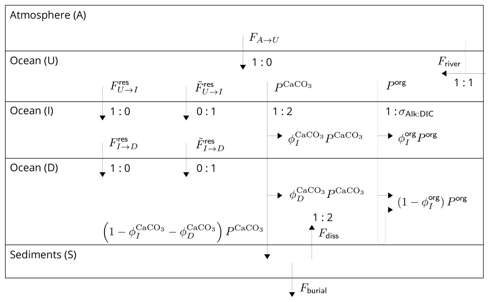
Figure 2 Schematic diagram of the DIC and Alk fluxes in SURFER v3.0. The ratios are ratios of DIC to alkalinity changes, i.e. an a:b ratio indicates that for a DIC change of a moles, there is an associated alkalinity change of b moles.

In the surface layer, calcifying organisms take up bicarbonate ions to form their calcium carbonate (CaCO₃) shells (forward Reaction R4).

$$\begin{array}{}\text{(R4)}& {\mathrm{Ca}}^{\mathrm{2}+}+\mathrm{2}{\mathrm{HCO}}_{\mathrm{3}}^{-}\rightleftharpoons {\mathrm{CO}}_{\mathrm{2}}+{\mathrm{H}}_{\mathrm{2}}\mathrm{O}+{\mathrm{CaCO}}_{\mathrm{3}}\end{array}$$

These organisms eventually die and sink to the ocean bottom. On the way down, some of the CaCO₃ is dissolved (reverse Reaction R4), resulting in downward transport of DIC and alkalinity at a 1:2 ratio. This is the carbonate pump. We represent the export of CaCO₃ at a depth of 150 m (so from layer U to I) by $P^{{\mathrm{CaCO}}_{\mathrm{3}}}$. A fraction, ${\mathit{\varphi }}_{\mathrm{I}}^{{\mathrm{CaCO}}_{\mathrm{3}}}$, of this export simultaneously dissolves in the intermediate layer (I), and a fraction, ${\mathit{\varphi }}_{\mathrm{D}}^{{\mathrm{CaCO}}_{\mathrm{3}}}$, simultaneously dissolves in the deep layer (D), which leaves a fraction, $\mathrm{1}-{\mathit{\varphi }}_{\mathrm{I}}^{{\mathrm{CaCO}}_{\mathrm{3}}}-{\mathit{\varphi }}_{\mathrm{D}}^{{\mathrm{CaCO}}_{\mathrm{3}}}$, reaching the sediments. Of the CaCO₃ that reaches the bottom of the ocean, some dissolves and some is permanently buried (details on this in Sect. 2.1.6).

In the surface layer, organisms also take up carbon through photosynthesis (primary production, forward Reaction R5).

$$\begin{array}{}\text{(R5)}& \begin{array}{rl}\mathrm{106}{\mathrm{CO}}_{\mathrm{2}}& +\mathrm{16}{\mathrm{NO}}_{\mathrm{3}}^{-}+{\mathrm{HPO}}_{\mathrm{4}}^{\mathrm{2}-}+\mathrm{122}{\mathrm{H}}_{\mathrm{2}}\mathrm{O}+\mathrm{18}{\mathrm{H}}^{+}\\ & \rightleftharpoons {\left({\mathrm{CH}}_{\mathrm{2}}\mathrm{O}\right)}_{\mathrm{106}}{\left({\mathrm{NH}}_{\mathrm{3}}\right)}_{\mathrm{16}}\left({\mathrm{H}}_{\mathrm{3}}{\mathrm{PO}}_{\mathrm{4}}\right)+\mathrm{138}{\mathrm{O}}_{\mathrm{2}}\end{array}\end{array}$$

The CO₂ is transformed into organic carbon that will eventually sink to the ocean bottom. On the way down, some of the organic carbon is re-mineralised (reverse Reaction R5), resulting in the downward transport of DIC. This is the soft-tissue pump (Volk and Hoffert, 1985). It also acts on alkalinity, mainly through the uptake and release of the H⁺ needed for the transformation of inorganic nitrate (NO${}_{\mathrm{3}}^{-}$) into organic nitrogen. Primary production of organic matter increases alkalinity, while re-mineralisation decreases alkalinity. We represent the ratio of alkalinity to DIC change for primary production and re-mineralisation with the parameter σ_Alk:DIC. We represent the export of organic carbon at a depth of 150 m (so from layer U to I) by P^org. We consider that all this organic carbon is simultaneously re-mineralised in the water column, with a fraction ${\mathit{\varphi }}_{\mathrm{I}}^{\mathrm{org}}$ re-mineralised in the intermediate layer (I) and a fraction ${\mathit{\varphi }}_{\mathrm{D}}^{\mathrm{org}}=\mathrm{1}-{\mathit{\varphi }}_{\mathrm{I}}^{\mathrm{org}}$ re-mineralised in the deep layer (D). In reality, some organic carbon accumulates on the sea floor sediments, where a large part is re-mineralised and only a small amount is permanently buried (Sarmiento and Gruber, 2006). Here, by setting ${\mathit{\varphi }}_{\mathrm{D}}^{\mathrm{org}}=\mathrm{1}-{\mathit{\varphi }}_{\mathrm{I}}^{\mathrm{org}}$, we neglect this burial and effectively consider all organic carbon falling on sediments to be re-mineralised.

Apart from the carbonate and soft-tissue pumps, forming the biological pumps, other processes are responsible for the transport of carbon between the ocean layers. Ocean circulation and mixing will propagate variations in DIC caused by spatial and temporal variations in air–sea gas exchanges. This was called the gas exchange pump by Sarmiento and Gruber (2006). For example, a component of the gas exchange pump is the solubility pump (Volk and Hoffert, 1985): cold waters have higher solubility and are thus enriched in CO₂; they are also denser and will sink at high latitudes, resulting in the downward transport of DIC. Besides, upwelling is responsible for the upward transport of DIC and alkalinity, which is necessary to counteract the carbonate and soft-tissue pumps (Goosse, 2015). We gather all the processes related to ocean circulation and mixing in the residual terms $F_{\mathrm{U}\to \mathrm{I}}^{\mathrm{res}}$, $F_{\mathrm{I}\to \mathrm{D}}^{\mathrm{res}}$, ${\stackrel{\mathrm{̃}}{F}}_{\mathrm{U}\to \mathrm{I}}^{\mathrm{res}}$, and ${\stackrel{\mathrm{̃}}{F}}_{\mathrm{I}\to \mathrm{D}}^{\mathrm{res}}$. We consider the residual fluxes of DIC and alkalinity to be independent because some processes such as the solubility pump only act on DIC.

Based on the above considerations, the masses of dissolved inorganic carbon and the mass of carbon in the sediments evolve according to the following equations:

$$\begin{array}{}\text{(29)}& {\displaystyle }& {\displaystyle \frac{\mathrm{d}{M}_{\mathrm{U}}}{\mathrm{d}t}}=F_{\mathrm{A}\to \mathrm{U}}-P^{{\mathrm{CaCO}}_{\mathrm{3}}}-P^{\mathrm{org}}-F_{\mathrm{U}\to \mathrm{I}}^{\mathrm{res}}+F_{\mathrm{river}},\text{(30)}& {\displaystyle }& {\displaystyle \frac{\mathrm{d}{M}_{\mathrm{I}}}{\mathrm{d}t}}={\mathit{\varphi }}_{\mathrm{I}}^{{\mathrm{CaCO}}_{\mathrm{3}}}{P}^{{\mathrm{CaCO}}_{\mathrm{3}}}+{\mathit{\varphi }}_{\mathrm{I}}^{\mathrm{org}}{P}^{\mathrm{org}}+F_{\mathrm{U}\to \mathrm{I}}^{\mathrm{res}}-F_{\mathrm{I}\to \mathrm{D}}^{\mathrm{res}},\text{(31)}& {\displaystyle }& {\displaystyle \frac{\mathrm{d}{M}_{\mathrm{D}}}{\mathrm{d}t}}={\mathit{\varphi }}_{\mathrm{D}}^{{\mathrm{CaCO}}_{\mathrm{3}}}{P}^{{\mathrm{CaCO}}_{\mathrm{3}}}+\left(\mathrm{1}-{\mathit{\varphi }}_{\mathrm{I}}^{\mathrm{org}}\right)P^{\mathrm{org}}+F_{\mathrm{I}\to \mathrm{D}}^{\mathrm{res}}+F_{\mathrm{diss}},\text{(32)}& {\displaystyle }& {\displaystyle \frac{\mathrm{d}{M}_{\mathrm{S}}}{\mathrm{d}t}}=\left(\mathrm{1}-{\mathit{\varphi }}_{\mathrm{I}}^{{\mathrm{CaCO}}_{\mathrm{3}}}-{\mathit{\varphi }}_{\mathrm{D}}^{{\mathrm{CaCO}}_{\mathrm{3}}}\right)P^{{\mathrm{CaCO}}_{\mathrm{3}}}-F_{\mathrm{diss}}-F_{\mathrm{burial}}.\end{array}$$

We recover Eqs. (1)–(10) by setting

$$\begin{array}{}\text{(33)}& {\displaystyle }& {\displaystyle }{F}_{\mathrm{U}\to \mathrm{I}}=F_{\mathrm{U}\to \mathrm{I}}^{{\mathrm{CaCO}}_{\mathrm{3}}}+F_{\mathrm{U}\to \mathrm{I}}^{\mathrm{org}}+F_{\mathrm{U}\to \mathrm{I}}^{\mathrm{res}},\text{(34)}& {\displaystyle }& {\displaystyle }{F}_{\mathrm{I}\to \mathrm{D}}=F_{\mathrm{I}\to \mathrm{D}}^{{\mathrm{CaCO}}_{\mathrm{3}}}+F_{\mathrm{I}\to \mathrm{D}}^{\mathrm{org}}+F_{\mathrm{I}\to \mathrm{D}}^{\mathrm{res}},\text{(35)}& {\displaystyle }& {\displaystyle }{F}_{\mathrm{acc}}=\left(\mathrm{1}-{\mathit{\varphi }}_{\mathrm{I}}^{{\mathrm{CaCO}}_{\mathrm{3}}}-{\mathit{\varphi }}_{\mathrm{D}}^{{\mathrm{CaCO}}_{\mathrm{3}}}\right)P^{{\mathrm{CaCO}}_{\mathrm{3}}}-F_{\mathrm{diss}},\end{array}$$

with the fluxes associated with the carbonate pump defined as

$$\begin{array}{}\text{(36)}& {\displaystyle }& {\displaystyle }{F}_{\mathrm{U}\to \mathrm{I}}^{{\mathrm{CaCO}}_{\mathrm{3}}}=P^{{\mathrm{CaCO}}_{\mathrm{3}}},\text{(37)}& {\displaystyle }& {\displaystyle }{F}_{\mathrm{I}\to \mathrm{D}}^{{\mathrm{CaCO}}_{\mathrm{3}}}=\left(\mathrm{1}-{\mathit{\varphi }}_{\mathrm{I}}^{{\mathrm{CaCO}}_{\mathrm{3}}}\right)P^{{\mathrm{CaCO}}_{\mathrm{3}}},\end{array}$$

and the fluxes associated with the soft-tissue pump defined as

$$\begin{array}{}\text{(38)}& {\displaystyle }& {\displaystyle }{F}_{\mathrm{U}\to \mathrm{I}}^{\mathrm{org}}=P^{\mathrm{org}},\text{(39)}& {\displaystyle }& {\displaystyle }{F}_{\mathrm{I}\to \mathrm{D}}^{\mathrm{org}}=\left(\mathrm{1}-{\mathit{\varphi }}_{\mathrm{I}}^{\mathrm{org}}\right)P^{\mathrm{org}}.\end{array}$$

Consequently, for the carbonate alkalinity fluxes, we have

$$\begin{array}{}\text{(40)}& {\displaystyle }& {\displaystyle }{\stackrel{\mathrm{̃}}{F}}_{\mathrm{U}\to \mathrm{I}}=\mathrm{2}\times F_{\mathrm{U}\to \mathrm{I}}^{{\mathrm{CaCO}}_{\mathrm{3}}}+{\mathit{\sigma }}_{\mathrm{Alk}:\mathrm{DIC}}\times F_{\mathrm{U}\to \mathrm{I}}^{\mathrm{org}}+{\stackrel{\mathrm{̃}}{F}}_{\mathrm{U}\to \mathrm{I}}^{\mathrm{res}},\text{(41)}& {\displaystyle }& {\displaystyle }{\stackrel{\mathrm{̃}}{F}}_{\mathrm{I}\to \mathrm{D}}=\mathrm{2}\times F_{\mathrm{I}\to \mathrm{D}}^{{\mathrm{CaCO}}_{\mathrm{3}}}+{\mathit{\sigma }}_{\mathrm{Alk}:\mathrm{DIC}}\times F_{\mathrm{I}\to \mathrm{D}}^{\mathrm{org}}+{\stackrel{\mathrm{̃}}{F}}_{\mathrm{I}\to \mathrm{D}}^{\mathrm{res}},\text{(42)}& {\displaystyle }& {\displaystyle }{\stackrel{\mathrm{̃}}{F}}_{\mathrm{acc}}=\mathrm{2}\times F_{\mathrm{acc}}.\end{array}$$

In the experiments presented here (Sects. 3 and 4), we keep $P^{{\mathrm{CaCO}}_{\mathrm{3}}}$, ${\mathit{\varphi }}_{\mathrm{I}}^{{\mathrm{CaCO}}_{\mathrm{3}}}$, ${\mathit{\varphi }}_{\mathrm{D}}^{{\mathrm{CaCO}}_{\mathrm{3}}}$, P^org, and ${\mathit{\varphi }}_{\mathrm{I}}^{\mathrm{org}}$ constant. This is an idealisation. Production and export of CaCO₃ and organic matter are biological processes and, in reality, depend on the temperature, pH, salinity, nutrient concentration and other properties of the ocean. For example, changes in primary production (and thus the export of organic matter) may have contributed to the CO₂ changes during the glacial–interglacial cycles (Kohfeld and Ridgwell, 2009). In the future, changes in the biological pumps are also possible and might lead to additional feedbacks in the carbon cycle (Henson et al., 2022; Planchat et al., 2024).

For the residual exchange terms, we adopt a linear formalism with exchange coefficients, similarly to in SURFER v2.0:

$$\begin{array}{}\text{(43)}& {\displaystyle }& {\displaystyle }{F}_{\mathrm{U}\to \mathrm{I}}^{\mathrm{res}}=k_{\mathrm{U}\to \mathrm{I}}{M}_{\mathrm{U}}-k_{\mathrm{I}\to \mathrm{U}}{M}_{\mathrm{I}},\text{(44)}& {\displaystyle }& {\displaystyle }{F}_{\mathrm{I}\to \mathrm{D}}^{\mathrm{res}}=k_{\mathrm{I}\to \mathrm{D}}{M}_{\mathrm{I}}-k_{\mathrm{D}\to \mathrm{I}}{M}_{\mathrm{D}},\text{(45)}& {\displaystyle }& {\displaystyle }{\stackrel{\mathrm{̃}}{F}}_{\mathrm{U}\to \mathrm{I}}^{\mathrm{res}}={\stackrel{\mathrm{̃}}{k}}_{\mathrm{U}\to \mathrm{I}}{\stackrel{\mathrm{̃}}{Q}}_{\mathrm{U}}-{\stackrel{\mathrm{̃}}{k}}_{\mathrm{I}\to \mathrm{U}}{\stackrel{\mathrm{̃}}{Q}}_{\mathrm{I}},\text{(46)}& {\displaystyle }& {\displaystyle }{\stackrel{\mathrm{̃}}{F}}_{\mathrm{I}\to \mathrm{D}}^{\mathrm{res}}={\stackrel{\mathrm{̃}}{k}}_{\mathrm{I}\to \mathrm{D}}{\stackrel{\mathrm{̃}}{Q}}_{\mathrm{I}}-{\stackrel{\mathrm{̃}}{k}}_{\mathrm{D}\to \mathrm{I}}{\stackrel{\mathrm{̃}}{Q}}_{\mathrm{D}}.\end{array}$$

2.1.6 F_acc, ${\stackrel{\mathrm{̃}}{F}}_{\mathrm{acc}}$, and F_burial

The CaCO₃ raining on the ocean floor either accumulates and gets buried in sediments or dissolves, depending on the saturation state of the ocean waters with respect to CO${}_{\mathrm{3}}^{\mathrm{2}-}$ (Archer et al., 1998; Zeebe and Westbroek, 2003). Typically, the upper ocean is supersaturated with CO${}_{\mathrm{3}}^{\mathrm{2}-}$ while the deeper ocean is undersaturated, mainly due to the pressure dependence of CaCO₃ solubility (Sarmiento and Gruber, 2006). This means that most of the accumulation in sediments will happen in a region above where most of the dissolution happens. A transition zone separates the accumulation and dissolution regions. The top boundary of the transition zone is the lysocline, defined as the depth where the calcium carbonate content of sediments starts to decrease sharply or, in other words, the depth below which the rate of dissolution of CaCO₃ starts to increase significantly. The bottom boundary of the transition zone is called the carbonate (or calcite) compensation depth (CCD) and is the depth at which the rate of CaCO₃ dissolution is equal to the rate of supply from the CaCO₃ rain. Below this depth, no CaCO₃ is preserved in the sediments. The depth of the transition zone varies between places and ocean basins but is generally between 3000 and 5000 m deep (Sarmiento and Gruber, 2006). We may thus safely consider that both dissolution and accumulation happen in the deep ocean layer (D) in our model and that is why we group both processes into a single term, F_acc, which can be positive or negative, with negative values indicating net dissolution.

Estimates indicate that carbonate accumulation in shallow waters may be comparable in magnitude to that occurring in open-ocean deep sediments (Milliman, 1993; Milliman and Droxler, 1996; Vecsei, 2004). However, shallow waters are characterised by significantly higher sedimentation rates, necessitating distinct models or parameterisations (Ridgwell and Hargreaves, 2007). Moreover, factors such as carbonate fixation by corals and algae must also be taken into account. Given the significant uncertainty surrounding these processes and the lack of reliable data to quantify them, we excluded them from our model. This approach is equivalent to assuming that CaCO₃ accumulation on shelves and the weathering flux required to balance it remain constant throughout the simulations (Archer et al., 1998; Ridgwell and Hargreaves, 2007) despite potential influences from human activities (Andersson and Mackenzie, 2004).

In the open-ocean deep sediments, the local dissolution rate depends on the concentration of CaCO₃ in the sediments and the saturation state of pore water around the sediments with respect to carbonate (Sarmiento and Gruber, 2006). We thus assume that the globally integrated dissolution flux is a function of two variables only: the deep-ocean mean concentration of CO${}_{\mathrm{3}}^{\mathrm{2}-}$ and the total mass of erodible CaCO₃ sediments. We use the following parameterisation:

$$\begin{array}{}\text{(47)}& \begin{array}{rl}& F_{\mathrm{diss}}=\\ & \left\{\begin{array}{ll}\left(\mathrm{1}-{\mathit{\varphi }}_{\mathrm{I}}^{{\mathrm{CaCO}}_{\mathrm{3}}}-{\mathit{\varphi }}_{\mathrm{D}}^{{\mathrm{CaCO}}_{\mathrm{3}}}\right)P^{{\mathrm{CaCO}}_{\mathrm{3}}}& \mathrm{if}{M}_{\mathrm{S}}=\mathrm{0}\mathrm{and}D>\left(\mathrm{1}-{\mathit{\varphi }}_{\mathrm{I}}^{{\mathrm{CaCO}}_{\mathrm{3}}}-{\mathit{\varphi }}_{\mathrm{D}}^{{\mathrm{CaCO}}_{\mathrm{3}}}\right)P^{{\mathrm{CaCO}}_{\mathrm{3}}},\\ D& \mathrm{otherwise},\end{array}\right.\end{array}\end{array}$$

with

$$\begin{array}{}\text{(48)}& \begin{array}{rl}D& =F_{\mathrm{diss},\mathrm{0}}+{\mathit{\alpha }}_{\mathrm{diss}}\left({\left[{\mathrm{CO}}_{\mathrm{3}}^{\mathrm{2}-}\right]}_{\mathrm{D}}-{\left[{\mathrm{CO}}_{\mathrm{3}}^{\mathrm{2}-}\right]}_{\mathrm{D}}\left(t_{\mathrm{PI}}\right)\right)\\ & +{\mathit{\beta }}_{\mathrm{diss}}\left(M_{\mathrm{S}}-M_{\mathrm{S}}\left(t_{\mathrm{PI}}\right)\right)+{\mathit{\gamma }}_{\mathrm{diss}}\left({\left[{\mathrm{CO}}_{\mathrm{3}}^{\mathrm{2}-}\right]}_{\mathrm{D}}\right.\\ & \left.-{\left[{\mathrm{CO}}_{\mathrm{3}}^{\mathrm{2}-}\right]}_{\mathrm{D}}\left(t_{\mathrm{PI}}\right)\right)\left(M_{\mathrm{S}}-M_{\mathrm{S}}\left(t_{\mathrm{PI}}\right)\right).\end{array}\end{array}$$

The first case in Eq. (47) indicates that if the erodible sediment reservoir is empty, the dissolution flux cannot exceed the CaCO₃ rain flux, regardless of the saturation state of the deep waters. The accumulation fluxes of DIC and alkalinity, F_acc and ${\stackrel{\mathrm{̃}}{F}}_{\mathrm{acc}}$, are then given by Eqs. (35) and (42). A similar parameterisation was proposed and tested in Archer et al. (1998), but they use the CO${}_{\mathrm{3}}^{\mathrm{2}-}$ concentration at a particular point in the deep Pacific and the mass of CaCO₃ in the bioturbated layer of the sediments as their two variables instead of the mean deep ocean CO${}_{\mathrm{3}}^{\mathrm{2}-}$ and the mass of erodible CaCO₃. They show that the parameterised version of their model is comparable to the non-parameterised one, except for a dissolution spike in the first 1000–2000 years following the fossil fuel emissions and CO₂ invasion into the ocean. We choose the coefficient of our parameterisation based on theirs. Details can be found in Sect. 2.4.1.

In the sediments, the bioturbated layer is the layer where sediments are mixed by biological activity (bioturbation). Dissolution only occurs in the top few centimetres near the sediment–ocean interface but can effectively reach deeper because of bioturbation (Sarmiento and Gruber, 2006). If the dissolution rate is greater than the rain rate of CaCO₃ on the sea floor, the sediments will lose CaCO₃ until the bioturbated layer becomes saturated with non-erodible material. At this point, dissolution stops and deeper carbonates are isolated from the carbon cycle. This explains why the effective reservoir of sediment carbonates to be accounted for here (M_S) has a limited size, which is estimated to be around 1600 PgC as of today (Archer et al., 1998). The erodible depth is defined as the lower boundary of the erodible sediment inventory (Archer et al., 1998). By definition, CaCO₃ sediments that move below the erodible depth will never be dissolved, and we say that they are buried. Locally, the burial rate depends on the rain rate of non-erodible material and the concentration of CaCO₃ in sediments at the erodible depth. We assume that the former is constant and that the total burial flux only depends on the total mass of erodible CaCO₃. We use the following linear parameterisation:

$$\begin{array}{}\text{(49)}& F_{\mathrm{burial}}={\mathit{\alpha }}_{\mathrm{burial}}{M}_{\mathrm{S}}.\end{array}$$

2.1.7 V, F_weathering, F_{river influx}, and ${\stackrel{\mathrm{̃}}{F}}_{\mathrm{river}\mathrm{influx}}$

Continental weathering of carbonate and silicate rocks can absorb CO₂ out of the atmosphere through the following reactions (Berner et al., 1983; Walker et al., 1981):

$$\begin{array}{}\text{(R6)}& {\displaystyle }& {\displaystyle }{\mathrm{CO}}_{\mathrm{2}}+{\mathrm{H}}_{\mathrm{2}}\mathrm{O}+{\mathrm{CaCO}}_{\mathrm{3}}\rightleftharpoons {\mathrm{Ca}}^{\mathrm{2}+}+\mathrm{2}{\mathrm{HCO}}_{\mathrm{3}}^{-},\text{(R7)}& {\displaystyle }& {\displaystyle }\mathrm{2}{\mathrm{CO}}_{\mathrm{2}}+{\mathrm{H}}_{\mathrm{2}}\mathrm{O}+{\mathrm{CaSiO}}_{\mathrm{3}}\rightleftharpoons {\mathrm{Ca}}^{\mathrm{2}+}+\mathrm{2}{\mathrm{HCO}}_{\mathrm{3}}^{-}+{\mathrm{SiO}}_{\mathrm{2}}.\end{array}$$

Let us consider $F_{{\mathrm{CaCO}}_{\mathrm{3}}}$ and $F_{{\mathrm{CaSiO}}_{\mathrm{3}}}$, the fluxes of Ca²⁺ produced by these two processes. For carbonate weathering (Reaction R6), the production of 1 mol of Ca²⁺ consumes 1 mol of carbon (CO₂) from the atmosphere and produces 2 mol of DIC and alkalinity that is transported by the rivers to the ocean. For the silicate weathering (Reaction R7), the production of 1 mol of Ca²⁺ consumes 2 mol of carbon (CO₂) from the atmosphere and produces 2 mol of DIC and alkalinity that is transported by the rivers to the ocean. Hence, we set

$$\begin{array}{}\text{(50)}& {\displaystyle }& {\displaystyle }{F}_{\mathrm{weathering}}=F_{{\mathrm{CaCO}}_{\mathrm{3}}}+\mathrm{2}{F}_{{\mathrm{CaSiO}}_{\mathrm{3}}}\text{(51)}& {\displaystyle }& {\displaystyle }{F}_{\mathrm{river}\mathrm{influx}}=\mathrm{2}{F}_{{\mathrm{CaCO}}_{\mathrm{3}}}+\mathrm{2}{F}_{{\mathrm{CaSiO}}_{\mathrm{3}}}\text{(52)}& {\displaystyle }& {\displaystyle }{F}_{\mathrm{river}\mathrm{influx}}^{\mathrm{alk}}=\mathrm{2}{F}_{{\mathrm{CaCO}}_{\mathrm{3}}}+\mathrm{2}{F}_{{\mathrm{CaSiO}}_{\mathrm{3}}}.\end{array}$$

As with alkalinity, we use PgC yr⁻¹ for $F_{{\mathrm{CaCO}}_{\mathrm{3}}}$ and $F_{{\mathrm{CaSiO}}_{\mathrm{3}}}$ even though they are defined as fluxes of Ca²⁺. To go from Tmol yr⁻¹ to PgC yr⁻¹, one just has to divide by the molar mass of carbon, $\mathrm{12}\times {\mathrm{10}}^{-\mathrm{3}}$ mol kg⁻¹.

For every 2 mol of DIC produced by carbonate weathering, 1 mol of carbon is taken from the atmosphere reservoir and 1 mol of carbon comes from carbonate rocks on land, which are not explicitly described as a reservoir in our model. This extra mole is thus treated as an external source of carbon, like volcanism. The carbon entering the ocean from weathering fluxes will eventually precipitate back as CaCO₃ in the sediments, which releases CO₂. Thus, the net effect of carbonate weathering is to transfer CaCO₃ from rocks on land to sediments in the ocean but with no long-term net effect on the atmospheric CO₂. On the other hand, since silicate weathering consumes 1 mol more of CO₂ from the atmosphere for the same Ca²⁺ flux, its net effect is to remove carbon from the atmosphere. At equilibrium, this net removal is compensated by volcanic outgassing.

The $F_{{\mathrm{CaCO}}_{\mathrm{3}}}$ and $F_{{\mathrm{CaSiO}}_{\mathrm{3}}}$ fluxes are not constant and depend on many factors (for a review, see Kump et al., 2000). For example, temperature affects the rates of Reactions R6 and R7, water run-off on land influences how much undersaturated water will come in contact with rocks for weathering, and vegetation may affect the acidity of soils and thus the rates of dissolution. Colbourn et al. (2013) provide parameterisations of all these processes for the model of terrestrial rock weathering RockGEM, which was included in the GENIE Earth system modelling framework. They showed that the temperature feedback was the dominant factor, and we choose to consider this one only, especially given that SURFER lacks a representation of the hydrological cycle. Following their parameterisation, we set

$$\begin{array}{}\text{(53)}& {\displaystyle }& {\displaystyle }{F}_{{\mathrm{CaCO}}_{\mathrm{3}}}=F_{{\mathrm{CaCO}}_{\mathrm{3}},\mathrm{0}}\left(\mathrm{1}+k_{\mathrm{Ca}}\mathit{\delta }{T}_{\mathrm{U}}\right),\text{(54)}& {\displaystyle }& {\displaystyle }{F}_{{\mathrm{CaSiO}}_{\mathrm{3}}}=F_{{\mathrm{CaSiO}}_{\mathrm{3}},\mathrm{0}}{e}^{k_{\mathrm{T}}\mathit{\delta }{T}_{\mathrm{U}}},\end{array}$$

where k_Ca and k_T are constants, and δT_U is the temperature anomaly of the upper ocean (and atmosphere) modelled by SURFER. This is also the parameterisation used by Lord et al. (2016) in their cGENIE simulations, which we will use as a basis for comparison with SURFER (see Sect. 3.4).

2.1.8 Methane

The evolution of the methane concentration in the atmosphere is mainly controlled by three processes: natural and anthropogenic emissions increase the CH₄ concentration, whereas oxidation into CO₂ decreases it (Saunois et al., 2020).

Anthropogenic emissions can be divided in two sources, fossil emissions ($E_{\mathrm{fossil}}^{{\mathrm{CH}}_{\mathrm{4}}}$) and land use emissions ($E_{\text{land use}}^{{\mathrm{CH}}_{\mathrm{4}}}$). Fossil emissions come from the industry sector and from the use and exploitation of fossil fuels. Land use emissions result from agriculture (rice production, cattle, etc.); agricultural waste burning; and the burning of biomass such as forests, grasslands, and peat. Natural emissions ($E_{\mathrm{natural}}^{{\mathrm{CH}}_{\mathrm{4}}}$) mainly come the from the anaerobic decomposition of organic matter in wetlands but also from freshwater systems, termites, and geological sources such as volcanoes, permafrost, and methane hydrates. For a detailed treatment of the different methane emissions, see Saunois et al. (2020). The rate of natural emissions may depend on temperature, and if they increase upon global warming, this could lead to positive feedbacks and eventually tipping points (Nisbet et al., 2023; Fewster et al., 2022; Archer et al., 2009). For simplicity, we assume constant natural emissions. To ensure the conservation of carbon, land use CH₄ emissions are taken from the land reservoir, while natural CH₄ emissions are taken directly from the CO₂ atmospheric reservoir of carbon. The reason for this difference is explained in the next section.

Oxidation of methane ($F_{{\mathrm{CH}}_{\mathrm{4}},\mathrm{ox}}$, Reaction R8) is the main sink of methane out of the atmosphere and releases CO₂:

$$\begin{array}{}\text{(R8)}& {\mathrm{CH}}_{\mathrm{4}}+\mathrm{2}{\mathrm{O}}_{\mathrm{2}}\to {\mathrm{CO}}_{\mathrm{2}}+\mathrm{2}{\mathrm{H}}_{\mathrm{2}}\mathrm{O}.\end{array}$$

We describe this as a simple decay process:

$$\begin{array}{}\text{(55)}& F_{{\mathrm{CH}}_{\mathrm{4}},\mathrm{ox}}=-{\displaystyle \frac{M_{\mathrm{A}}^{{\mathrm{CH}}_{\mathrm{4}}}}{{\mathit{\tau }}_{{\mathrm{CH}}_{\mathrm{4}}}}},\end{array}$$

where ${\mathit{\tau }}_{{\mathrm{CH}}_{\mathrm{4}}}$ is the atmospheric CH₄ lifetime. In principle, it may vary depending on temperature and on the availability of the hydroxyl radical, OH, which is necessary for the intermediate steps of Reaction R8 and which itself depends on the concentrations of CH₄, N₂O, CO, and other trace gases (Skeie et al., 2023). However, for simplicity, we choose to keep ${\mathit{\tau }}_{{\mathrm{CH}}_{\mathrm{4}}}$ constant and set its value to 9.5 yr. We add the product of oxidation to M_A.

2.1.9 Land reservoir and land use emissions

In SURFER v3.0, we distinguish greenhouse gas emissions caused by fossil fuel use from those caused by land use. While fossil CO₂ and CH₄ emissions are directly added to the atmosphere, land use CO₂ and CH₄ emissions ($E_{\text{land use}}^{{\mathrm{CO}}_{\mathrm{2}}}$ and $E_{\text{land use}}^{{\mathrm{CH}}_{\mathrm{4}}}$) must be taken from the land reservoir (Eq. 3). In SURFER v2.0, based on the outputs of the Zero Emissions Commitment Model Intercomparison Project (ZECMIP) experiments (Jones et al., 2019; MacDougall et al., 2020), we parameterised the carbon flux from the land to the atmosphere in the following way:

$$\begin{array}{}\text{(56)}& \begin{array}{rl}{F}_{\mathrm{A}\to \mathrm{L}}& =k_{\mathrm{A}\to \mathrm{L}}({\mathit{\beta }}_{\mathrm{L}}{M}_{\mathrm{A}\left(t_{\mathrm{PI}}\right)}\left(\mathrm{1}-{\displaystyle \frac{M_{\mathrm{A}}\left(t_{\mathrm{PI}}\right)}{M_{\mathrm{A}}}}\right)\\ & -\left(M_{\mathrm{L}}-M_{\mathrm{L}}\left(t_{\mathrm{PI}}\right)\right)).\end{array}\end{array}$$

This is equivalent to saying that M_L relaxes to an equilibrium mass $M_{\mathrm{L}}^{\mathrm{eq}}\left(M_{\mathrm{A}}\right)$ equal to

$$\begin{array}{}\text{(57)}& M_{\mathrm{L}}^{\mathrm{eq}}\left(M_{\mathrm{A}}\right)={\mathit{\beta }}_{\mathrm{L}}{M}_{\mathrm{A}}\left(t_{\mathrm{PI}}\right)\left(\mathrm{1}-{\displaystyle \frac{M_{\mathrm{A}}\left(t_{\mathrm{PI}}\right)}{M_{\mathrm{A}}}}\right)+M_{\mathrm{L}}\left(t_{\mathrm{PI}}\right),\end{array}$$

with a timescale $\mathrm{1}/k_{\mathrm{A}\to \mathrm{L}}$.

Now suppose that we have a certain amount of land use emissions; we transfer some carbon from the land reservoir to the atmosphere reservoir and let the model evolve without changing anything else. Then the F_A→L flux, as it is, will increase and the land will absorb the carbon lost until the initial equilibrium is reached again. Physically, this means that the forest that was replaced by grassland or crop fields has grown back to its original size. In the real world, this may happen, but if the land is managed (e.g. for agriculture), the forest does not regrow. To take this into account, we subtract the cumulative CO₂ land use emissions from the equilibrium mass to which M_L relaxes,

$$\begin{array}{}\text{(58)}& \begin{array}{rl}{M}_{\mathrm{L}}^{\mathrm{eq}}\left(M_{\mathrm{A}},t\right)& ={\mathit{\beta }}_{\mathrm{L}}{M}_{\mathrm{A}\left(t_{\mathrm{PI}}\right)}\left(\mathrm{1}-{\displaystyle \frac{M_{\mathrm{A}}\left(t_{\mathrm{PI}}\right)}{M_{\mathrm{A}}}}\right)+M_{\mathrm{L}}\left(t_{\mathrm{PI}}\right)\\ & -\underset{t_{\mathrm{0}}}{\overset{t}{\int }}{E}_{\text{land use}}^{{\mathrm{CO}}_{\mathrm{2}}}\left(t\right).\end{array}\end{array}$$

This is the same procedure as in the model from Lenton (2000), except that they subtract only a fraction of the cumulative land use emissions, allowing for some forest regrowth. Here we subtract all land use emissions because, in principle, the negative emissions coming from forest regrowth should already be accounted for in the net reported land use emissions (IPCC, 2021a, p. 688). We can rewrite the new F_A→L flux as

$$\begin{array}{}\text{(59)}& \begin{array}{rl}{F}_{\mathrm{A}\to \mathrm{L}}& =k_{\mathrm{A}\to \mathrm{L}}({\mathit{\beta }}_{\mathrm{L}}{M}_{\mathrm{A}\left(t_{\mathrm{PI}}\right)}\left(\mathrm{1}-{\displaystyle \frac{M_{\mathrm{A}}\left(t_{\mathrm{PI}}\right)}{M_{\mathrm{A}}}}\right)\\ & -\left(M_{\mathrm{L}}-M_{\mathrm{L}}^{*}\right)),\end{array}\end{array}$$

where $M_{\mathrm{L}}^{*}$ is a new model variable, the evolution of which is described by

$$\begin{array}{}\text{(60)}& {\displaystyle \frac{\mathrm{d}{M}_{\mathrm{L}}^{*}}{\mathrm{d}t}}=-E_{\text{land use}}^{{\mathrm{CO}}_{\mathrm{2}}}\left(t\right),\end{array}$$

with $M_{\mathrm{L}}^{*}\left(t_{\mathrm{PI}}\right)=M_{\mathrm{L}}\left(t_{\mathrm{PI}}\right)$.

We have not included methane land use emissions in Eqs. (58)–(60). This means that the carbon mass in CH₄ form taken from the land reservoir is reabsorbed by the land once methane is oxidised back to CO₂. In other words, methane land use emissions do not cause a net addition of CO₂ in the atmosphere through oxidation. This makes sense if you consider methane emissions coming from the anaerobic decomposition of organic matter in rice cultures or cattle stomachs. Indeed, the decomposed organic matter was formed not too long before by absorbing CO₂ from the atmosphere through photosynthesis, so when the methane oxidises into CO₂, it closes the loop and there is no net effect on atmospheric CO₂.

The same reasoning applies to most natural emissions of methane that arise from wetlands: they do not cause a net increase in atmospheric CO₂ concentrations. In principle, these natural methane emissions should be subtracted from the land carbon reservoir as anthropogenic land use emissions, and there should be a nonzero atmosphere-to-land equilibrium flux that compensates for the CO₂ created from oxidation. However, this is impossible with our parameterisation of the atmosphere-to-land flux, which is zero at preindustrial times by construction. To avoid introducing yet another parameterisation or a more detailed representation of the carbon on land and to maintain carbon conservation, we merely subtract the natural emissions directly from the CO₂ mass of carbon in the atmosphere. This approach is justified by our assumption that the natural methane production–oxidation cycle is in equilibrium.

Natural CH₄ emissions coming from geological processes such as volcanism or natural-gas leaks would have a net impact on CO₂ levels, but they are negligible compared to emissions coming from wetlands (Saunois et al., 2020). Natural CH₄ emissions coming from permafrost would also have a lasting effect on CO₂ concentrations because the organic matter from which they originate was formed thousands of years before. Accounting for emissions from permafrost would require yet another parameterisation, and we instead neglected them in SURFER v3.0.

2.2 Climate component

The equations for the climate component are essentially the same as in SURFER v2.0, with the addition of an oceanic box and the radiative forcing due to methane. The atmosphere is considered to be in thermal equilibrium with the surface-ocean layer (U). The evolution of temperature anomalies for the three oceanic layers is dictated by

$$\begin{array}{}\text{(61)}& {\displaystyle }\begin{array}{rl}{c}_{\mathrm{vol}}{h}_{\mathrm{U}}{\displaystyle \frac{\mathrm{d}\mathit{\delta }{T}_{\mathrm{U}}}{\mathrm{d}t}}& =F\left(M_{\mathrm{A}},M_{\mathrm{A}}^{{\mathrm{CH}}_{\mathrm{4}}},I\right)-\mathit{\beta }\mathit{\delta }{T}_{\mathrm{U}}\\ & -{\mathit{\gamma }}_{\mathrm{U}\to \mathrm{I}}\left(\mathit{\delta }{T}_{\mathrm{U}}-\mathit{\delta }{T}_{\mathrm{I}}\right),\end{array}\text{(62)}& {\displaystyle }{c}_{\mathrm{vol}}{h}_{\mathrm{I}}{\displaystyle \frac{\mathrm{d}\mathit{\delta }{T}_{\mathrm{I}}}{\mathrm{d}t}}={\mathit{\gamma }}_{\mathrm{U}\to \mathrm{I}}\left(\mathit{\delta }{T}_{\mathrm{U}}-\mathit{\delta }{T}_{\mathrm{I}}\right)-{\mathit{\gamma }}_{\mathrm{I}\to \mathrm{D}}\left(\mathit{\delta }{T}_{\mathrm{I}}-\mathit{\delta }{T}_{\mathrm{D}}\right),\text{(63)}& {\displaystyle }{c}_{\mathrm{vol}}{h}_{\mathrm{D}}{\displaystyle \frac{\mathrm{d}\mathit{\delta }{T}_{\mathrm{D}}}{\mathrm{d}t}}={\mathit{\gamma }}_{\mathrm{I}\to \mathrm{D}}\left(\mathit{\delta }{T}_{\mathrm{I}}-\mathit{\delta }{T}_{\mathrm{D}}\right),\end{array}$$

where $F(M_{\mathrm{A}},M_{\mathrm{A}}^{{\mathrm{CH}}_{\mathrm{4}}},I)$ is the anthropogenic radiative forcing. Its expression is given by

$$\begin{array}{}\text{(64)}& \begin{array}{rl}F\left(M_{\mathrm{A}},M_{\mathrm{A}}^{{\mathrm{CH}}_{\mathrm{4}}},I\right)& =F_{\mathrm{2}\times }{\log }_{\mathrm{2}}\left({\displaystyle \frac{M_{\mathrm{A}}}{M_{\mathrm{A}}\left(t_{\mathrm{PI}}\right)}}\right)\\ & +{\mathit{\alpha }}_{{\mathrm{CH}}_{\mathrm{4}}}\sqrt{M_{\mathrm{A}}^{{\mathrm{CH}}_{\mathrm{4}}}-M_{\mathrm{A}}^{{\mathrm{CH}}_{\mathrm{4}}}\left(t_{\mathrm{PI}}\right)}\\ & -{\mathit{\alpha }}_{{\mathrm{SO}}_{\mathrm{2}}}\exp \left(-{\left({\mathit{\beta }}_{{\mathrm{SO}}_{\mathrm{2}}}/I\right)}^{\mathit{\gamma }{\mathrm{SO}}_{\mathrm{2}}}\right).\end{array}\end{array}$$

The first two terms describe the contribution of CO₂ and methane to an increased greenhouse effect. The third term corresponds to solar radiation modification in the form of SO₂ injections (Martínez Montero et al., 2022).

2.3 Sea level rise component

Sea level rise is estimated as the sum of four contributions: thermal expansion and melt from the mountain glaciers, the Greenland ice sheet, and the Antarctic ice sheet.

$$\begin{array}{}\text{(65)}& S_{\mathrm{tot}}=S_{\mathrm{th}}+S_{\mathrm{gl}}+S_{\mathrm{GIS}}+S_{\mathrm{AIS}}\end{array}$$

Compared to SURFER v2.0, we only change the parameterisation of thermal expansion, where we need to add a term to take into account the new intermediate layer.

$$\begin{array}{}\text{(66)}& S_{\mathrm{th}}={\mathit{\alpha }}_{\mathrm{U}}{h}_{\mathrm{U}}\mathit{\delta }{T}_{\mathrm{U}}+{\mathit{\alpha }}_{\mathrm{I}}{h}_{\mathrm{I}}\mathit{\delta }{T}_{\mathrm{I}}+{\mathit{\alpha }}_{\mathrm{D}}{h}_{\mathrm{D}}\mathit{\delta }{T}_{\mathrm{D}}\end{array}$$

Here α_i is the thermal expansion coefficient corresponding to layer $i\in \mathit{\{}\mathrm{U},\mathrm{I},\mathrm{D}\mathit{\}}$. The other contributions are the same as in Martínez Montero et al. (2022). We recall them here, and more details are provided in the original publication.

The evolution of the sea level rise contribution from glaciers is given by the equation

$$\begin{array}{}\text{(67)}& {\displaystyle \frac{\mathrm{d}{S}_{\mathrm{gl}}}{\mathrm{d}t}}={\displaystyle \frac{\mathrm{1}}{{\mathit{\tau }}_{\mathrm{gl}}}}\left(S_{\mathrm{gleq}}\left(\mathit{\delta }{T}_{\mathrm{U}}\right)-S_{\mathrm{gl}}\right),\end{array}$$

with

$$\begin{array}{}\text{(68)}& S_{\mathrm{gleq}}\left(\mathit{\delta }{T}_{\mathrm{U}}\right)=S_{\mathrm{gl}\mathrm{pot}}\tanh \left({\displaystyle \frac{\mathit{\delta }{T}_{\mathrm{U}}}{\mathit{\zeta }}}\right).\end{array}$$

Here τ_gl is a relaxation timescale, S_gl pot is the potential sea level rise due to mountain glaciers, and ζ is a sensitivity coefficient.

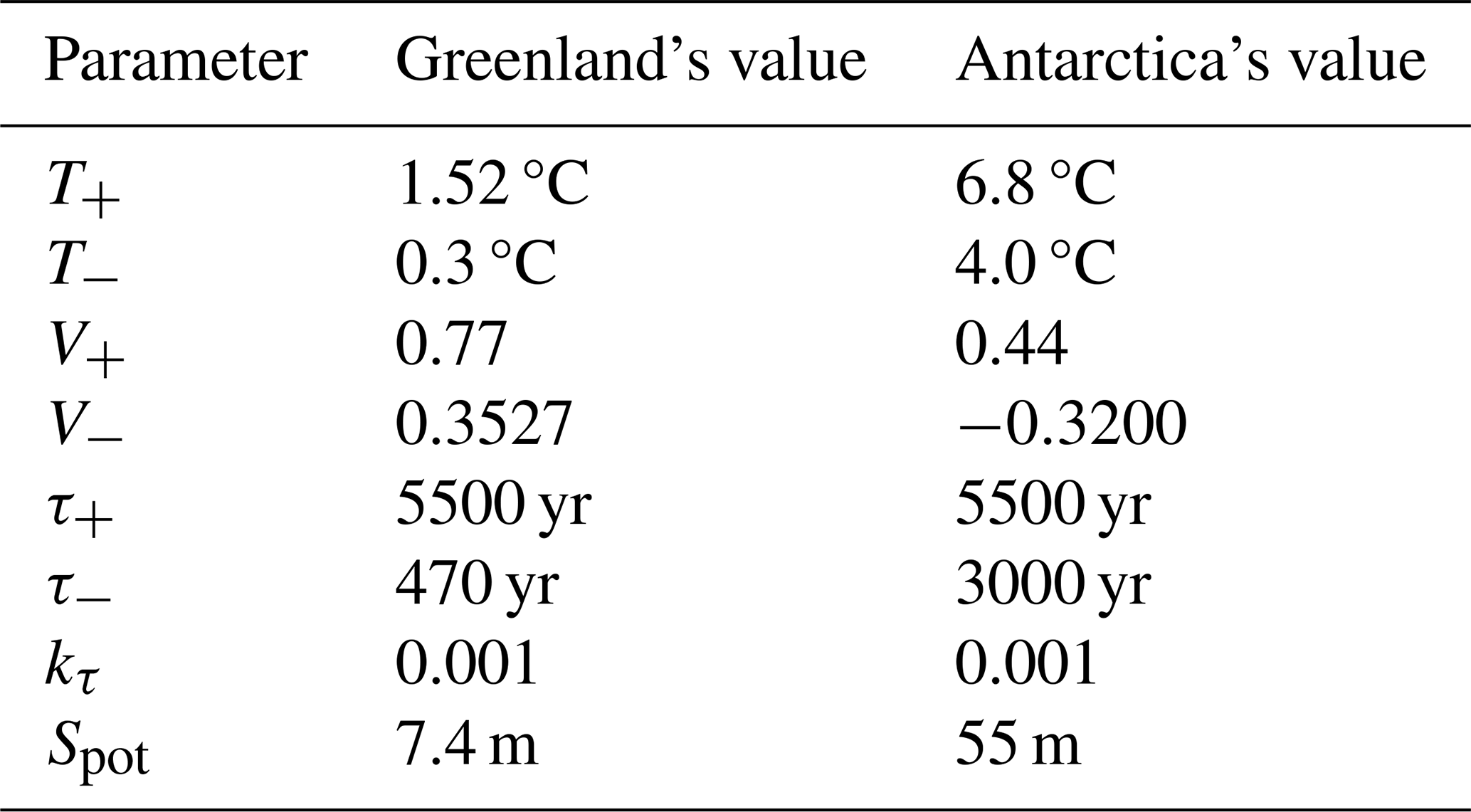
The contributions from Greenland and Antarctica are given by

$$\begin{array}{}\text{(69)}& S_{\mathrm{GIS}}=S_{\mathrm{GIS}}\left(\mathrm{1}-V_{\mathrm{GIS}}\left(t\right)\right),S_{\mathrm{AIS}}=S_{\mathrm{AIS}}\left(\mathrm{1}-V_{\mathrm{AIS}}\left(t\right)\right),\end{array}$$

where S_GIS and S_AIS are the sea level rise potential of the Greenland and Antarctic ice sheets, and V_GIS and V_AIS are the volume fractions of the ice sheets with respect to their preindustrial volumes. The evolution of ice sheet volumes is described by the equation

$$\begin{array}{}\text{(70)}& {\displaystyle \frac{\mathrm{d}V}{\mathrm{d}t}}=\mathit{\mu }\left(V,\mathit{\delta }{T}_{\mathrm{U}}\right)\underset{H}{\underbrace{\left(-V^{\mathrm{3}}+a_{\mathrm{2}}{V}^{\mathrm{2}}+a_{\mathrm{1}}V+c_{\mathrm{1}}\mathit{\delta }{T}_{\mathrm{U}}+c_{\mathrm{0}}\right)}},\end{array}$$

with

$$\begin{array}{}\text{(71)}& \mathit{\mu }\left(V,\mathit{\delta }{T}_{\mathrm{U}}\right)=\left\{\begin{array}{ll}\mathrm{1}/\mathit{\tau }& \mathrm{if}H>\mathrm{0}\mathrm{or}(H<\mathrm{0}\mathrm{and}V>\mathrm{0}),\\ \mathrm{0}& \mathrm{if}H<\mathrm{0}\mathrm{and}V=\mathrm{0},\end{array}\right.\end{array}$$

and

$$\begin{array}{}\text{(72)}& \mathit{\tau }={\mathit{\tau }}_{-}+{\displaystyle \frac{{\mathit{\tau }}_{+}-{\mathit{\tau }}_{-}}{\mathrm{2}}}\left(\mathrm{1}+\tanh \left({\displaystyle \frac{H}{k_{\mathit{\tau }}}}\right)\right).\end{array}$$

The timescales τ₊ and τ₋ are associated with the asymmetric processes of freezing and melting. The first case in Eq. (71) was separated into two cases in SURFER v2.0, depending on the sign of H. In SURFER v3.0, we introduce a smooth transition between τ₊ and τ₋ when H changes sign. This formulation effectively prevents small fluctuations around the equilibrium having different timescales (when H is close to zero). The parameter k_τ controls the smoothness of the transition, with k_τ=∞ corresponding to the discontinuous step transition used in SURFER v2.0. The constant parameters (a₂, a₁, c₁, c₀) are given in terms of (T₊, V₊), (T₋, V₋), which are the bifurcation points of the steady-state structure induced by Eq. (70):

$$\begin{array}{}\text{(73)}& {\displaystyle }& {\displaystyle }{a}_{\mathrm{2}}={\displaystyle \frac{\mathrm{3}\left(V_{-}+V_{+}\right)}{\mathrm{2}}},\text{(74)}& {\displaystyle }& {\displaystyle }{a}_{\mathrm{1}}=-\mathrm{3}{V}_{-}{V}_{+},\text{(75)}& {\displaystyle }& {\displaystyle }{c}_{\mathrm{1}}=-{\displaystyle \frac{{\left(V_{+}-V_{-}\right)}^{\mathrm{3}}}{\mathrm{2}\left(T_{+}-T_{-}\right)}},\text{(76)}& {\displaystyle }& {\displaystyle }{c}_{\mathrm{0}}=+{\displaystyle \frac{T_{+}{V}_{-}^{\mathrm{2}}\left(V_{-}-\mathrm{3}{V}_{+}\right)-T_{-}{V}_{+}^{\mathrm{2}}\left(V_{+}-\mathrm{3}{V}_{-}\right)}{\mathrm{2}\left(T_{-}-T_{+}\right)}}.\end{array}$$

These relationships allow SURFER to be easily calibrated on the steady-state structure of more complex ice sheet models.

2.4 Calibration and initial conditions

We calibrate the parameters and initial conditions of the model using known physics, observations, model results, and the hypothesis that the carbon cycle was at equilibrium during preindustrial times. This follows standard practice, even though processes involving longer timescales active at glacial–interglacial timescales are not necessarily in balance (Brovkin et al., 2016). We assume

$$\begin{array}{}\text{(77)}& {\displaystyle }\begin{array}{rl}\mathrm{0}& =V-F_{\mathrm{A}\to \mathrm{U}}\left(t_{\mathrm{PI}}\right)-F_{\mathrm{A}\to \mathrm{L}}\left(t_{\mathrm{PI}}\right)+F_{{\mathrm{CH}}_{\mathrm{4}},\mathrm{ox}}\left(t_{\mathrm{PI}}\right)\\ & -E_{\mathrm{nat}}^{{\mathrm{CH}}_{\mathrm{4}}}-F_{\mathrm{weathering}}\left(t_{\mathrm{PI}}\right),\end{array}\text{(78)}& {\displaystyle }\mathrm{0}=E_{\mathrm{nat}}^{{\mathrm{CH}}_{\mathrm{4}}}-F_{{\mathrm{CH}}_{\mathrm{4}},\mathrm{ox}}\left(t_{\mathrm{PI}}\right),\text{(79)}& {\displaystyle }\mathrm{0}=F_{\mathrm{A}\to \mathrm{L}}\left(t_{\mathrm{PI}}\right),\text{(80)}& {\displaystyle }\mathrm{0}=F_{\mathrm{A}\to \mathrm{U}}\left(t_{\mathrm{PI}}\right)-F_{\mathrm{U}\to \mathrm{I}}\left(t_{\mathrm{PI}}\right)+F_{\mathrm{river}}\left(t_{\mathrm{PI}}\right),\text{(81)}& {\displaystyle }\mathrm{0}=F_{\mathrm{U}\to \mathrm{I}}\left(t_{\mathrm{PI}}\right)-F_{\mathrm{I}\to \mathrm{D}}\left(t_{\mathrm{PI}}\right),\text{(82)}& {\displaystyle }\mathrm{0}=F_{\mathrm{I}\to \mathrm{D}}\left(t_{\mathrm{PI}}\right)-F_{\mathrm{acc}}\left(t_{\mathrm{PI}}\right),\text{(83)}& {\displaystyle }\mathrm{0}=-{\stackrel{\mathrm{̃}}{F}}_{\mathrm{U}\to \mathrm{I}}\left(t_{\mathrm{PI}}\right)+{\stackrel{\mathrm{̃}}{F}}_{\mathrm{river}}\left(t_{\mathrm{PI}}\right),\text{(84)}& {\displaystyle }\mathrm{0}={\stackrel{\mathrm{̃}}{F}}_{\mathrm{U}\to \mathrm{I}}\left(t_{\mathrm{PI}}\right)-{\stackrel{\mathrm{̃}}{F}}_{\mathrm{I}\to \mathrm{D}}\left(t_{\mathrm{PI}}\right),\text{(85)}& {\displaystyle }\mathrm{0}={\stackrel{\mathrm{̃}}{F}}_{\mathrm{I}\to \mathrm{D}}\left(t_{\mathrm{PI}}\right)-{\stackrel{\mathrm{̃}}{F}}_{\mathrm{acc}}\left(t_{\mathrm{PI}}\right),\text{(86)}& {\displaystyle }\mathrm{0}=F_{\mathrm{acc}}\left(t_{\mathrm{PI}}\right)-F_{\mathrm{burial}}\left(t_{\mathrm{PI}}\right).\end{array}$$

From Eqs. (83)–(85), we get ${\stackrel{\mathrm{̃}}{F}}_{\mathrm{acc}}\left(t_{\mathrm{PI}}\right)={\stackrel{\mathrm{̃}}{F}}_{\mathrm{I}\to \mathrm{D}}\left(t_{\mathrm{PI}}\right)={\stackrel{\mathrm{̃}}{F}}_{\mathrm{U}\to \mathrm{I}}\left(t_{\mathrm{PI}}\right)={\stackrel{\mathrm{̃}}{F}}_{\mathrm{river}}\left(t_{\mathrm{PI}}\right)=\mathrm{2}{F}_{{\mathrm{CaCO}}_{\mathrm{3}},\mathrm{0}}+\mathrm{2}{F}_{{\mathrm{CaSiO}}_{\mathrm{3}},\mathrm{0}}$. The dissolution and precipitation of CaCO₃ produces and consumes moles of DIC and alkalinity at a 1:2 ratio (see Sect. 2.1.6); hence we have $F_{\mathrm{acc}}\left(t_{\mathrm{PI}}\right)=\frac{\mathrm{1}}{\mathrm{2}}{\stackrel{\mathrm{̃}}{F}}_{\mathrm{acc}}\left(t_{\mathrm{PI}}\right)=F_{{\mathrm{CaCO}}_{\mathrm{3}},\mathrm{0}}+F_{{\mathrm{CaSiO}}_{\mathrm{3}},\mathrm{0}}$. We then get $F_{\mathrm{U}\to \mathrm{I}}\left(t_{\mathrm{PI}}\right)=F_{\mathrm{I}\to \mathrm{D}}\left(t_{\mathrm{PI}}\right)=F_{\mathrm{burial}}\left(t_{\mathrm{PI}}\right)=F_{\mathrm{acc}}\left(t_{\mathrm{PI}}\right)=F_{{\mathrm{CaCO}}_{\mathrm{3}},\mathrm{0}}+F_{{\mathrm{CaSiO}}_{\mathrm{3}},\mathrm{0}}$ from Eqs. (81), (82), and (86). Equation (80) gives us $F_{\mathrm{A}\to \mathrm{L}}\left(t_{\mathrm{PI}}\right)=-(F_{{\mathrm{CaCO}}_{\mathrm{3}},\mathrm{0}}+F_{{\mathrm{CaSiO}}_{\mathrm{3}},\mathrm{0}})$, Eq. (78) tells us that $E_{\mathrm{nat}}^{{\mathrm{CH}}_{\mathrm{4}}}=F_{{\mathrm{CH}}_{\mathrm{4}},\mathrm{ox}}\left(t_{\mathrm{PI}}\right)$, and finally, from Eq. (77), we find $V=F_{{\mathrm{CaSiO}}_{\mathrm{3}},\mathrm{0}}$. Equation (79) provides no extra information since $F_{\mathrm{A}\to \mathrm{L}}\left(t_{\mathrm{PI}}\right)=\mathrm{0}$ by construction. Developing the expressions of the carbon fluxes, we get the following system of equations:

$$\begin{array}{}\text{(87)}& {\displaystyle }V=F_{{\mathrm{CaSiO}}_{\mathrm{3}},\mathrm{0}},\text{(88)}& {\displaystyle }{E}_{\mathrm{nat}}^{{\mathrm{CH}}_{\mathrm{4}}}={\displaystyle \frac{M_{\mathrm{A}}^{{\mathrm{CH}}_{\mathrm{4}}}\left(t_{\mathrm{PI}}\right)}{{\mathit{\tau }}_{{\mathrm{CH}}_{\mathrm{4}}}}},\text{(89)}& {\displaystyle }\mathrm{0}=\mathrm{0},\text{(90)}& {\displaystyle }\begin{array}{rl}{\stackrel{\mathrm{‾}}{k}}_{\mathrm{A}\to \mathrm{U}}{K}_{\mathrm{0}}(M_{\mathrm{A}}\left(t_{\mathrm{PI}}\right)& -{\displaystyle \frac{m_{\mathrm{A}}}{W_{\mathrm{U}}{K}_{\mathrm{0}}}}{M}_{\mathrm{U}}^{\prime }\left(t_{\mathrm{PI}}\right))\\ & =-\left(F_{{\mathrm{CaCO}}_{\mathrm{3}},\mathrm{0}}+F_{{\mathrm{CaSiO}}_{\mathrm{3}},\mathrm{0}}\right),\end{array}\text{(91)}& {\displaystyle }\begin{array}{rl}{P}^{{\mathrm{CaCO}}_{\mathrm{3}}}& +P^{\mathrm{org}}+k_{\mathrm{U}\to \mathrm{I}}{M}_{\mathrm{U}}\left(t_{\mathrm{PI}}\right)-k_{\mathrm{I}\to \mathrm{U}}{M}_{\mathrm{I}}\left(t_{\mathrm{PI}}\right)\\ & =F_{{\mathrm{CaCO}}_{\mathrm{3}},\mathrm{0}}+F_{{\mathrm{CaSiO}}_{\mathrm{3}},\mathrm{0}},\end{array}\text{(92)}& {\displaystyle }\begin{array}{rl}\left(\mathrm{1}-{\mathit{\varphi }}_{\mathrm{I}}^{{\mathrm{CaCO}}_{\mathrm{3}}}\right)P^{{\mathrm{CaCO}}_{\mathrm{3}}}& +\left(\mathrm{1}-{\mathit{\varphi }}_{\mathrm{I}}^{\mathrm{org}}\right)P^{\mathrm{org}}\\ & +k_{\mathrm{I}\to \mathrm{D}}{M}_{\mathrm{I}}\left(t_{\mathrm{PI}}\right)-k_{\mathrm{D}\to \mathrm{I}}{M}_{\mathrm{D}}\left(t_{\mathrm{PI}}\right)\\ & =F_{{\mathrm{CaCO}}_{\mathrm{3}},\mathrm{0}}+F_{{\mathrm{CaSiO}}_{\mathrm{3}},\mathrm{0}},\end{array}\end{array}$$

$$\begin{array}{}\text{(93)}& {\displaystyle }\begin{array}{rl}\mathrm{2}{P}^{{\mathrm{CaCO}}_{\mathrm{3}}}& +{\mathit{\sigma }}_{\mathrm{Alk}:\mathrm{DIC}}{P}^{\mathrm{org}}+{\stackrel{\mathrm{̃}}{k}}_{\mathrm{U}\to \mathrm{I}}{\stackrel{\mathrm{̃}}{Q}}_{\mathrm{U}}\left(t_{\mathrm{PI}}\right)\\ & -{\stackrel{\mathrm{̃}}{k}}_{\mathrm{I}\to \mathrm{U}}{\stackrel{\mathrm{̃}}{Q}}_{\mathrm{I}}\left(t_{\mathrm{PI}}\right)=\mathrm{2}\left(F_{{\mathrm{CaCO}}_{\mathrm{3}},\mathrm{0}}+F_{{\mathrm{CaSiO}}_{\mathrm{3}},\mathrm{0}}\right),\end{array}\text{(94)}& {\displaystyle }\begin{array}{rl}\mathrm{2}\left(\mathrm{1}-{\mathit{\varphi }}_{\mathrm{I}}^{{\mathrm{CaCO}}_{\mathrm{3}}}\right)P^{{\mathrm{CaCO}}_{\mathrm{3}}}& +{\mathit{\sigma }}_{\mathrm{Alk}:\mathrm{DIC}}\left(\mathrm{1}-{\mathit{\varphi }}_{\mathrm{I}}^{\mathrm{org}}\right)P^{\mathrm{org}}\\ & +{\stackrel{\mathrm{̃}}{k}}_{\mathrm{I}\to \mathrm{D}}{\stackrel{\mathrm{̃}}{Q}}_{\mathrm{I}}\left(t_{\mathrm{PI}}\right)-{\stackrel{\mathrm{̃}}{k}}_{\mathrm{D}\to \mathrm{I}}{\stackrel{\mathrm{̃}}{Q}}_{\mathrm{D}}\left(t_{\mathrm{PI}}\right)\\ & =\mathrm{2}\left(F_{{\mathrm{CaCO}}_{\mathrm{3}},\mathrm{0}}+F_{{\mathrm{CaSiO}}_{\mathrm{3}},\mathrm{0}}\right),\end{array}\text{(95)}& {\displaystyle }\begin{array}{rl}\left(\mathrm{1}-{\mathit{\varphi }}_{\mathrm{I}}^{{\mathrm{CaCO}}_{\mathrm{3}}}\right.& \left.-{\mathit{\varphi }}_{\mathrm{D}}^{{\mathrm{CaCO}}_{\mathrm{3}}}\right)P^{{\mathrm{CaCO}}_{\mathrm{3}}}-F_{\mathrm{diss},\mathrm{0}}=F_{{\mathrm{CaCO}}_{\mathrm{3}},\mathrm{0}}\\ & +F_{{\mathrm{CaSiO}}_{\mathrm{3}},\mathrm{0}},\end{array}\text{(96)}& {\displaystyle }{\mathit{\alpha }}_{\mathrm{burial}}{M}_{\mathrm{S}}\left(t_{\mathrm{PI}}\right)=F_{{\mathrm{CaCO}}_{\mathrm{3}},\mathrm{0}}+F_{{\mathrm{CaSiO}}_{\mathrm{3}},\mathrm{0}}.\end{array}$$

The equilibrium hypothesis effectively provides us with constraints linking some parameters and initial conditions. In Sect. 2.4.1, we discuss the choice and calibration of the model parameters. A sensitivity analysis for most parameters is presented in Appendix D. In Sect. 2.4.2, we provide a set of initial conditions for the model.

2.4.1 Parameters

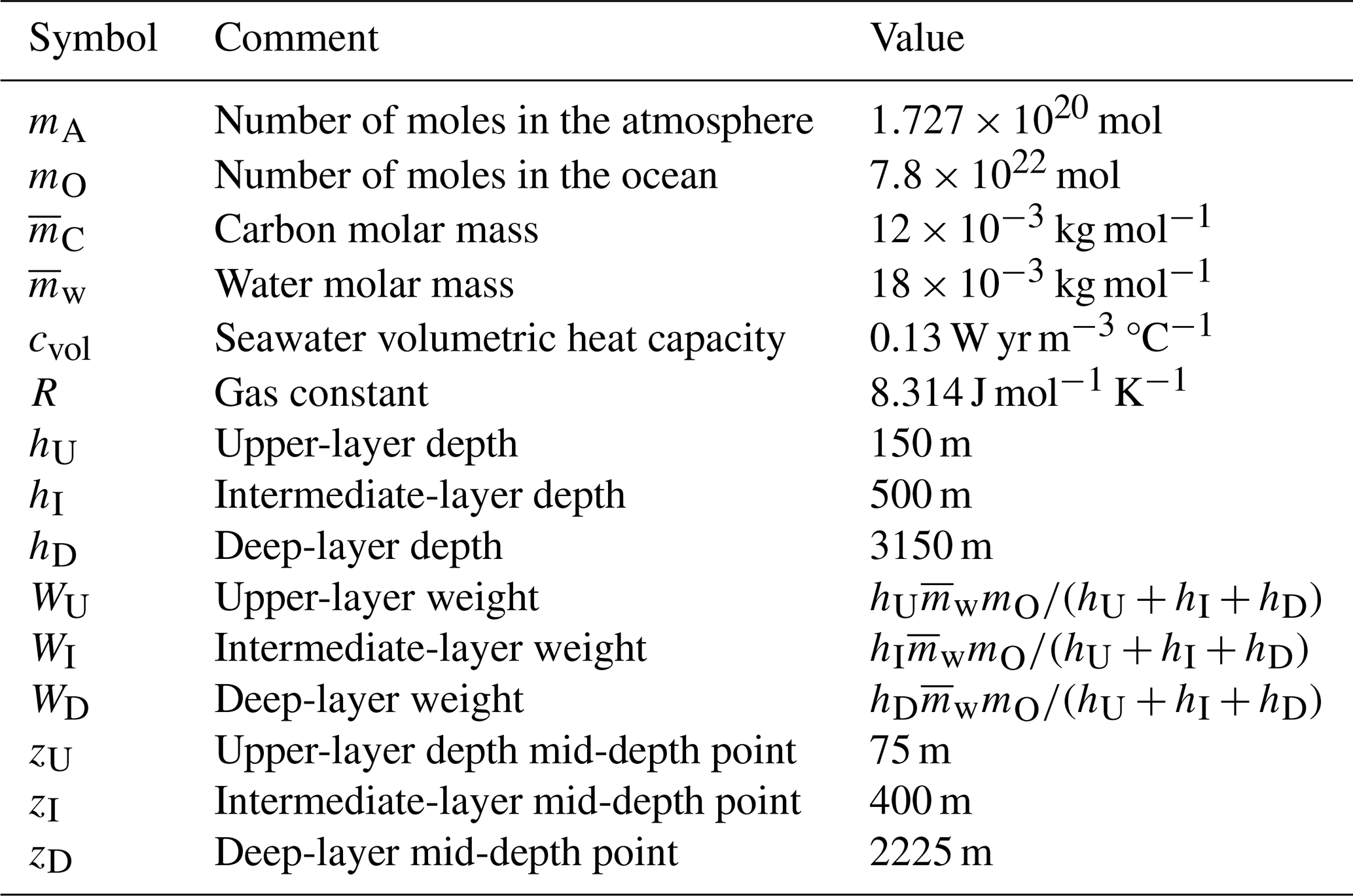
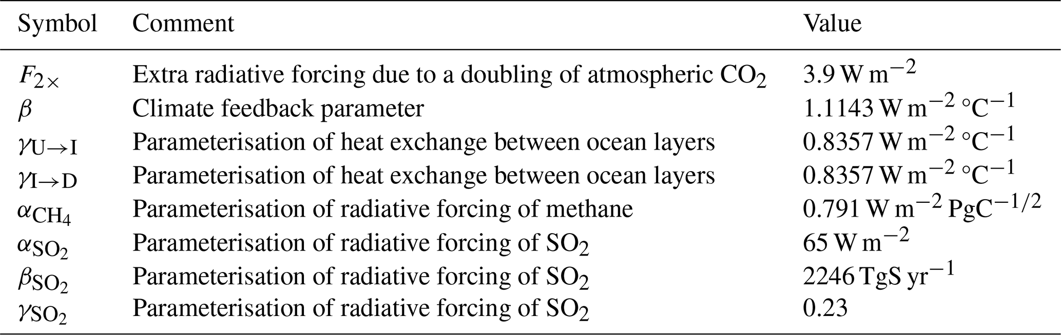
The values of the parameters representing physical quantities and constants, as well as those defining the model's geometry, are given in Table 1.

Table 1 Physical parameters and geometry.

Carbon cycle component

The parameters that control the CO₂ uptake by vegetation (β_L, k_A→L) and the CO₂ uptake by the ocean on short timescales (k_U→I and ${\stackrel{\mathrm{̃}}{k}}_{\mathrm{U}\to \mathrm{I}}$) are tuned to reproduce historical observations of CO₂ concentrations (Fig. 4), historical estimations of land and ocean sinks (Fig. 6), and historical and Shared Socioeconomic Pathway (SSP) runs from CMIP6 (Figs. 7 and 8). The parameters k_I→D and ${\stackrel{\mathrm{̃}}{k}}_{\mathrm{I}\to \mathrm{D}}$, which control the ocean carbon uptake on multicentennial to multimillennial timescales, are chosen to produce a reasonable fit to the 1 Myr runs of cGENIE (see Sect. 3.4). Overall, the calibration to other models is performed qualitatively, without optimising well-defined metrics.

The parameter ${\stackrel{\mathrm{‾}}{k}}_{\mathrm{A}\to \mathrm{U}}$ is defined as ${\stackrel{\mathrm{‾}}{k}}_{\mathrm{A}\to \mathrm{U}}=A_{\mathrm{O}}\mathit{\rho }k/m_{\mathrm{A}}$. With ocean area $A_{\mathrm{O}}=\mathrm{361}\times {\mathrm{10}}^{\mathrm{12}}$ m², mean seawater density ρ=1026 kg m⁻³, gas transfer velocity 20 cm $h^{-\mathrm{1}}=\mathrm{0.2}\cdot \mathrm{365}\cdot \mathrm{24}$ m yr⁻¹ (Yang et al., 2022), and the number of moles in the atmosphere $m_{\mathrm{A}}=\mathrm{1.727}\times {\mathrm{10}}^{\mathrm{20}}$ mol, we obtain ${\stackrel{\mathrm{‾}}{k}}_{\mathrm{A}\to \mathrm{U}}=\mathrm{4.7}$ kg (mol yr)⁻¹. The parameter β_L, which controls the amount of CO₂ uptake by vegetation (see Eq. 59), is set to 1.7. This is the same value as for SURFER v2.0, which was calibrated on the outputs of the ZECMIP experiments (Jones et al., 2019). The parameter k_A→L is set to 0.044, which is an increase by a factor 1.75 compared to SURFER v2.0. This is done to have a better match with historical CO₂ concentrations.

The parameters that dictate the DIC and alkalinity exchanges between the ocean layers are physically determined by the oceanic circulation; hence we expect them to be similar ($k_{i\to j}\approx {\stackrel{\mathrm{̃}}{k}}_{i\to j}$ for $i,j\in \mathit{\{}\mathrm{U},\mathrm{I},\mathrm{D}\mathit{\}}$), but we do not require them to be equal because some processes such as the solubility pump can impact DIC and alkalinity independently. Yet for simplicity, we set both k_U→I and ${\stackrel{\mathrm{̃}}{k}}_{\mathrm{U}\to \mathrm{I}}$ to 0.13 yr⁻¹ and both k_I→D and ${\stackrel{\mathrm{̃}}{k}}_{\mathrm{I}\to \mathrm{D}}$ to 0.009 yr⁻¹. Then, k_I→U, ${\stackrel{\mathrm{̃}}{k}}_{\mathrm{I}\to \mathrm{U}}$, k_D→I, and ${\stackrel{\mathrm{̃}}{k}}_{\mathrm{D}\to \mathrm{I}}$ are computed from Eqs. (91)–(94). We have

$$\begin{array}{}\text{(97)}& {\displaystyle }\begin{array}{rl}{k}_{\mathrm{I}\to \mathrm{U}}& =\left(P^{{\mathrm{CaCO}}_{\mathrm{3}}}+P^{\mathrm{org}}-\left(F_{{\mathrm{CaCO}}_{\mathrm{3}},\mathrm{0}}+F_{{\mathrm{CaSiO}}_{\mathrm{3}},\mathrm{0}}\right)\right.\\ & +k_{\mathrm{U}\to \mathrm{I}}{M}_{\mathrm{U}}\left(t_{\mathrm{PI}}\right)){\displaystyle \frac{\mathrm{1}}{M_{\mathrm{I}}\left(t_{\mathrm{PI}}\right)}},\end{array}\text{(98)}& {\displaystyle }\begin{array}{rl}{k}_{\mathrm{D}\to \mathrm{I}}& =(\left(\mathrm{1}-{\mathit{\varphi }}_{\mathrm{I}}^{{\mathrm{CaCO}}_{\mathrm{3}}}\right)P^{{\mathrm{CaCO}}_{\mathrm{3}}}+\left(\mathrm{1}-{\mathit{\varphi }}_{\mathrm{I}}^{\mathrm{org}}\right)P^{\mathrm{org}}\\ & -\left(F_{{\mathrm{CaCO}}_{\mathrm{3}},\mathrm{0}}+F_{{\mathrm{CaSiO}}_{\mathrm{3}},\mathrm{0}}\right)+k_{\mathrm{I}\to \mathrm{D}}{M}_{\mathrm{I}}\left(t_{\mathrm{PI}}\right))\\ & {\displaystyle \frac{\mathrm{1}}{M_{\mathrm{D}}\left(t_{\mathrm{PI}}\right)}},\end{array}\text{(99)}& {\displaystyle }\begin{array}{rl}{\stackrel{\mathrm{̃}}{k}}_{\mathrm{I}\to \mathrm{U}}& =\left(\mathrm{2}{P}^{{\mathrm{CaCO}}_{\mathrm{3}}}+{\mathit{\sigma }}_{\mathrm{Alk}:\mathrm{DIC}}{P}^{\mathrm{org}}-\mathrm{2}\left(F_{{\mathrm{CaCO}}_{\mathrm{3}},\mathrm{0}}\right.\right.\\ & \left.\left.+F_{{\mathrm{CaSiO}}_{\mathrm{3}},\mathrm{0}}\right)+{\stackrel{\mathrm{̃}}{k}}_{\mathrm{U}\to \mathrm{I}}{\stackrel{\mathrm{̃}}{Q}}_{\mathrm{U}}\left(t_{\mathrm{PI}}\right)\right){\displaystyle \frac{\mathrm{1}}{{\stackrel{\mathrm{̃}}{Q}}_{\mathrm{I}}\left(t_{\mathrm{PI}}\right)}},\end{array}\text{(100)}& {\displaystyle }\begin{array}{rl}{\stackrel{\mathrm{̃}}{k}}_{\mathrm{D}\to \mathrm{I}}=& \left(\mathrm{2}\left(\mathrm{1}-{\mathit{\varphi }}_{\mathrm{I}}^{{\mathrm{CaCO}}_{\mathrm{3}}}\right)P^{{\mathrm{CaCO}}_{\mathrm{3}}}+{\mathit{\sigma }}_{\mathrm{Alk}:\mathrm{DIC}}\right.\\ & \left(\mathrm{1}-{\mathit{\varphi }}_{\mathrm{I}}^{\mathrm{org}}\right)P^{\mathrm{org}}-\mathrm{2}\left(F_{{\mathrm{CaCO}}_{\mathrm{3}},\mathrm{0}}+F_{{\mathrm{CaSiO}}_{\mathrm{3}},\mathrm{0}}\right)\\ & \left.+{\stackrel{\mathrm{̃}}{k}}_{\mathrm{I}\to \mathrm{D}}{\stackrel{\mathrm{̃}}{Q}}_{\mathrm{I}}\left(t_{\mathrm{PI}}\right)\right){\displaystyle \frac{\mathrm{1}}{{\stackrel{\mathrm{̃}}{Q}}_{\mathrm{D}}\left(t_{\mathrm{PI}}\right)}}.\end{array}\end{array}$$

With the choices for the other parameters described hereafter, we obtain $k_{\mathrm{I}\to \mathrm{U}}=\mathrm{0.0383}$ yr⁻¹, ${\stackrel{\mathrm{̃}}{k}}_{\mathrm{I}\to \mathrm{U}}=\mathrm{0.0392}$ yr⁻¹, $k_{\mathrm{D}\to \mathrm{I}}=\mathrm{1.44}\times {\mathrm{10}}^{-\mathrm{3}}$ yr⁻¹, and ${\stackrel{\mathrm{̃}}{k}}_{\mathrm{D}\to \mathrm{I}}=\mathrm{1.43}\times {\mathrm{10}}^{-\mathrm{3}}$ yr⁻¹. Overall, this corresponds to a timescale range of 7.7–26.1 yr ($\mathrm{1}/k_{\mathrm{U}\to \mathrm{I}}-\mathrm{1}/k_{\mathrm{I}\to \mathrm{U}}$) for the oceanic carbon exchanges between the surface and intermediate layers and a timescale range of 111.1–693.8 yr ($\mathrm{1}/k_{\mathrm{I}\to \mathrm{D}}-\mathrm{1}/k_{\mathrm{D}\to \mathrm{I}}$) for the oceanic carbon exchanges between the intermediate and deep layers. This also gives preindustrial DIC fluxes of 175 PgC yr⁻¹ for subduction (k_U→IM_U(t_PI)) and 183 PgC yr⁻¹ for obduction (k_I→UM_I(t_PI)). Although these carbon fluxes are an order of magnitude greater than the fluxes from the biological pumps, they are much less frequently studied, and estimates in the literature are rare. IPCC AR5 gave estimates of 90 and 101 PgC yr⁻¹ for subduction and obduction, respectively (Stocker et al., 2013), while IPCC AR6 gave estimates of 264 and 275 PgC yr⁻¹ (Levy et al., 2013; Canadell et al., 2021).

The CaCO₃ export from the ocean surface has been estimated between 0.6 and 1.8 PgC yr⁻¹ (see Supplement in Sulpis et al., 2021, and references therein). Sulpis et al. (2021) provide a tighter range of 0.77 to 1.06 PgC yr⁻¹, of which 0.34 to 0.53 PgC yr⁻¹ are dissolved in the water column before reaching the sediments. We set $P^{{\mathrm{CaCO}}_{\mathrm{3}}}$ to 1 PgC yr⁻¹, which is also the value given in Sarmiento and Gruber (2006) for the open-ocean export at a 100 m depth. We set ${\mathit{\varphi }}_{\mathrm{I}}^{{\mathrm{CaCO}}_{\mathrm{3}}}=\mathrm{0.15}$ and ${\mathit{\varphi }}_{\mathrm{D}}^{{\mathrm{CaCO}}_{\mathrm{3}}}=\mathrm{0.39}$. This gives us a total of 0.54 PgC yr⁻¹ dissolved in the water column and 0.46 PgC yr⁻¹ that rains on the sediments, which is close to estimates from Sulpis et al. (2021) and Sarmiento and Gruber (2006, see Fig. 9.1.1).

Estimates of the export of organic carbon out of the euphotic zone range from 4 to 12 PgC yr⁻¹ (DeVries and Weber, 2017, and references therein). The euphotic zone is the uppermost layer of the ocean that receives sunlight and where photosynthesis can happen. Since the re-mineralisation of organic matter is quite fast in the water column, estimates of carbon export vary greatly depending on the specific definition of the euphotic zone and its depth. Based on a data-assimilated model, DeVries and Weber (2017) give an estimate of 9.1±0.2 PgC yr⁻¹ for the organic carbon export out of the euphotic zone and an estimate of 6.7 PgC yr⁻¹ for the organic carbon export at 100 m in depth. In our model, we set the organic carbon export P^org at a 150 m depth to 7 PgC yr⁻¹, which corresponds to the estimate given for the open ocean in Sarmiento and Gruber (2006), and we set ${\mathit{\varphi }}_{\mathrm{I}}^{\mathrm{org}}=\mathrm{0.72}$. Reaction (R5) suggests that for a 106 mol decrease in DIC due to organic matter production, alkalinity will increase by 17 mol (the uptake of 18 mol of H⁺ increases alkalinity by 18 mol, while the uptake of HPO${}_{\mathrm{4}}^{\mathrm{2}-}$, which is one of the minor bases included in the full definition of alkalinity (Eq. 12), decreases alkalinity by 1 mol). Here, we follow Sarmiento and Gruber (2006) and set σ_Alk:DIC to $-\mathrm{16}/\mathrm{117}$, meaning that for 1 mol uptake of DIC in organic matter production, alkalinity is increased by $\mathrm{16}/\mathrm{117}=\mathrm{0.14}$ mol. Setting ${\mathit{\sigma }}_{\mathrm{Alk}:\mathrm{DIC}}=-\mathrm{16}/\mathrm{117}$ instead of ${\mathit{\sigma }}_{\mathrm{Alk}:\mathrm{DIC}}=-\mathrm{17}/\mathrm{106}$ does not result in much change, as can be seen from the sensitivity analysis in Appendix D.

For our parameterisation of CaCO₃ dissolution, we need to calibrate four parameters. The value of F_diss,0 is computed using equilibrium conditions. From Eq. (95), we obtain

$$\begin{array}{}\text{(101)}& \begin{array}{rl}{F}_{\mathrm{diss},\mathrm{0}}& =\left(\mathrm{1}-{\mathit{\varphi }}_{\mathrm{I}}^{{\mathrm{CaCO}}_{\mathrm{3}}}-{\mathit{\varphi }}_{\mathrm{D}}^{{\mathrm{CaCO}}_{\mathrm{3}}}\right)P^{{\mathrm{CaCO}}_{\mathrm{3}}}\\ & -\left(F_{{\mathrm{CaCO}}_{\mathrm{3}},\mathrm{0}}+F_{{\mathrm{CaSiO}}_{\mathrm{3}},\mathrm{0}}\right).\end{array}\end{array}$$

With the choice of $P^{{\mathrm{CaCO}}_{\mathrm{3}}}$, ${\mathit{\varphi }}_{\mathrm{I}}^{{\mathrm{CaCO}}_{\mathrm{3}}}$, and ${\mathit{\varphi }}_{\mathrm{D}}^{{\mathrm{CaCO}}_{\mathrm{3}}}$ described above and the choice for $F_{{\mathrm{CaCO}}_{\mathrm{3}},\mathrm{0}}$ and $F_{{\mathrm{CaSiO}}_{\mathrm{3}},\mathrm{0}}$ described below, we get $F_{\mathrm{diss},\mathrm{0}}=\mathrm{0.33}$ PgC yr⁻¹. The parameters α_diss, β_diss, and γ_diss are obtained based on a parameterisation provided in Archer et al. (1998) for accumulation (rain minus dissolution). The values we use are given in Table 2.

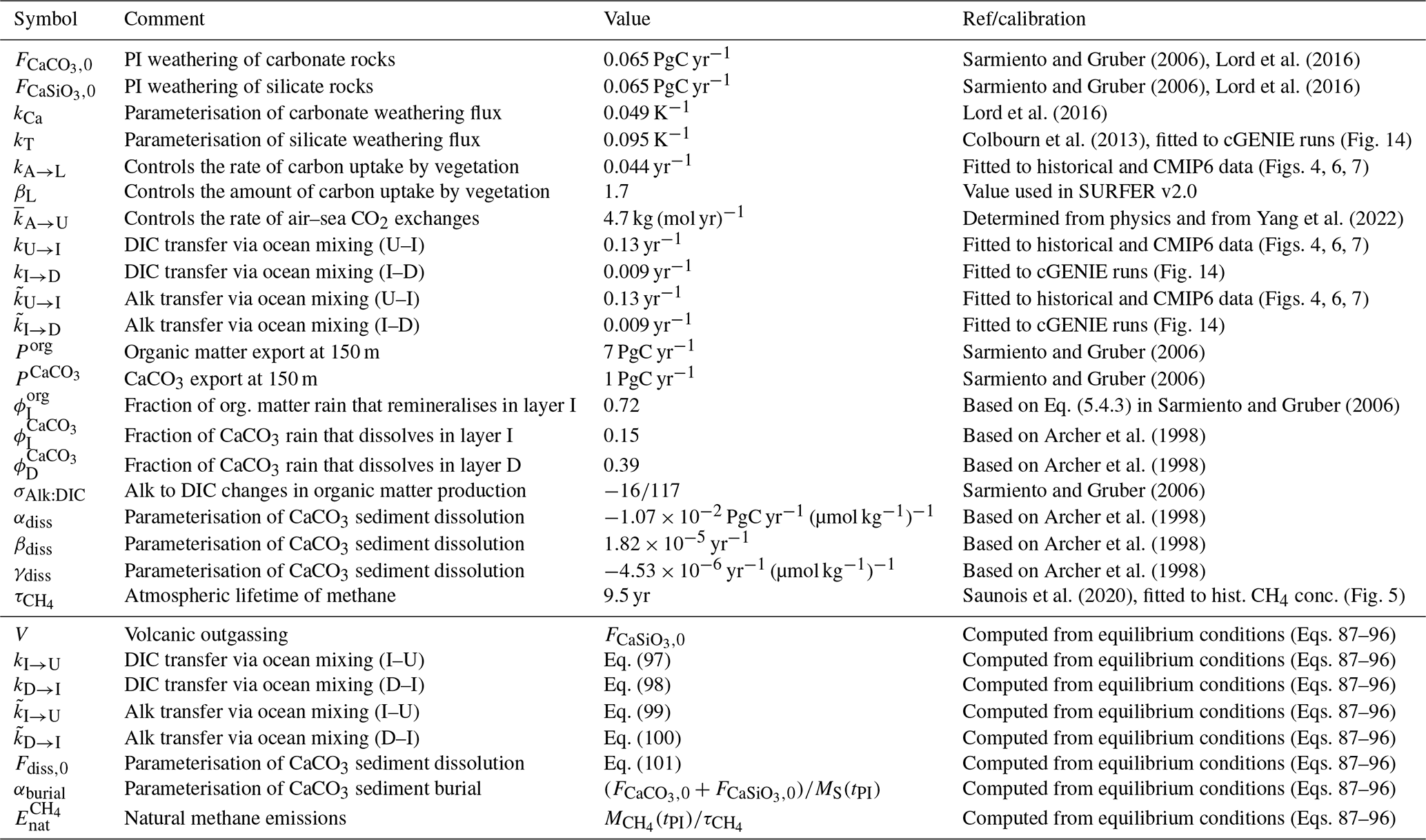
Sarmiento and Gruber (2006)Lord et al. (2016)Sarmiento and Gruber (2006)Lord et al. (2016)Lord et al. (2016)Colbourn et al. (2013)Yang et al. (2022)Sarmiento and Gruber (2006)Sarmiento and Gruber (2006)Sarmiento and Gruber (2006)Archer et al. (1998)Archer et al. (1998)Sarmiento and Gruber (2006)Archer et al. (1998)Archer et al. (1998)Archer et al. (1998)Saunois et al. (2020)

Table 2 Parameters for the carbon cycle component. The rightmost column lists references used for parameter tuning and, where applicable, the calibration targets to which the parameters were fitted. The calibration to other models is performed qualitatively, without optimising well-defined metrics.

We split the total weathering flux evenly between silicate and carbonate weathering ($F_{{\mathrm{CaCO}}_{\mathrm{3}},\mathrm{0}}=F_{{\mathrm{CaSiO}}_{\mathrm{3}},\mathrm{0}}$), and we set them to obtain a preindustrial burial flux of 0.13 PgC yr⁻¹. This is the estimate given in Sarmiento and Gruber (2006). For comparison, the IPCC gives an estimate of 0.2 PgC yr⁻¹ (Canadell et al., 2021). From Eq. (89), we have $F_{{\mathrm{CaCO}}_{\mathrm{3}},\mathrm{0}}+F_{{\mathrm{CaSiO}}_{\mathrm{3}},\mathrm{0}}={\mathit{\alpha }}_{\mathrm{burial}}{M}_{\mathrm{S}}\left(t_{\mathrm{PI}}\right)=F_{\mathrm{burial}}\left(t_{\mathrm{PI}}\right)=\mathrm{0.13}$ PgC yr⁻¹, which gives us $F_{{\mathrm{CaCO}}_{\mathrm{3}},\mathrm{0}}=F_{{\mathrm{CaSiO}}_{\mathrm{3}},\mathrm{0}}=\mathrm{0.065}$ PgC yr⁻¹ or 5.42 Tmol yr⁻¹. This implies preindustrial CO₂ consumption fluxes of 5.42 Tmol yr⁻¹ for carbonate weathering ($F_{{\mathrm{CaCO}}_{\mathrm{3}},\mathrm{0}}$) and 10.84 Tmol yr⁻¹ for silicate weathering ($\mathrm{2}\times F_{{\mathrm{CaSiO}}_{\mathrm{3}},\mathrm{0}}$). These values are relatively low compared to the literature estimates of 8.6–12.3 and 11.7–17.9 Tmol yr⁻¹, respectively (Colbourn et al., 2015, and references therein). Nevertheless, they are close to the values from Lord et al. (2016), whose 1 Myr cGENIE runs we use as a calibration target for SURFER v3.0. This being said, setting higher preindustrial weathering fluxes, and in particular higher carbonate weathering fluxes, has a minimal impact on simulated atmospheric CO₂ concentrations, as demonstrated in Appendix D.

From these choices, we get ${\mathit{\alpha }}_{\mathrm{burial}}=(F_{{\mathrm{CaCO}}_{\mathrm{3}},\mathrm{0}}+F_{{\mathrm{CaSiO}}_{\mathrm{3}},\mathrm{0}})/M_{\mathrm{S}}\left(t_{\mathrm{PI}}\right)=\mathrm{0.13}/M_{\mathrm{S}}\left(t_{\mathrm{PI}}\right)$. Volcanic outgassing is set to $V=F_{{\mathrm{CaSiO}}_{\mathrm{3}},\mathrm{0}}=\mathrm{0.065}$ PgC yr⁻¹ as per Eq. (87). The IPCC estimate is 0.1 PgC yr⁻¹. Following Colbourn et al. (2013), we set k_Ca to 0.049 K⁻¹ and k_T to

$$\begin{array}{}\text{(102)}& k_{\mathrm{T}}={\displaystyle \frac{\mathrm{1000}{E}_{\mathrm{a}}}{R{T}_{\mathrm{0}}^{\mathrm{2}}}},\end{array}$$

where R is the gas constant (in J K⁻¹ mol⁻¹), T₀ is the global mean preindustrial temperature (in K), and E_a is the activation energy for dissolution (in kJ mol⁻¹). West et al. (2005) provide an estimate for the activation energy: $E_{\mathrm{a}}=\mathrm{74}\pm \mathrm{29}$ kJ mol⁻¹. With $T_{\mathrm{0}}=T_{\mathrm{U}}\left(t_{\mathrm{PI}}\right)=\mathrm{288.38}$ K (as set in Sect. 2.4.2), this gives a range for k_T between 0.065 and 0.149 K⁻¹. We set k_T=0.095 K⁻¹. Together with the other parameter choices, this leads to long-term CO₂ atmospheric concentrations that fit the ones simulated by Lord et al. (2016) with cGENIE well (see Sect. 3.4). We note that more recent work has provided updated estimates for the action energy E_a as low as 22 kJ mol⁻¹, which would imply lower values for k_T than the ones we are using (Brantley et al., 2023). On the other hand, using a higher value may help compensate for the absence of a simulated hydrological cycle, which is critical for representing silicate and carbonate weathering fluxes but whose response to anthropogenic emissions is less certain than that of temperature (Kukla et al., 2023; Maher and Chamberlain, 2014).

Natural methane emissions are set to $E_{\mathrm{nat}}^{{\mathrm{CH}}_{\mathrm{4}}}=M_{\mathrm{A}}^{{\mathrm{CH}}_{\mathrm{4}}}\left(t_{\mathrm{PI}}\right)/{\mathit{\tau }}_{{\mathrm{CH}}_{\mathrm{4}}}$. With $M_{\mathrm{A}}^{{\mathrm{CH}}_{\mathrm{4}}}\left(t_{\mathrm{PI}}\right)$ chosen as in Sect. 2.4.2 and ${\mathit{\tau }}_{{\mathrm{CH}}_{\mathrm{4}}}=\mathrm{9.5}$ yr, we get natural emissions of 0.157 PgC yr⁻¹ or 209 Tg CH₄ yr⁻¹. This is in the range of the top-down estimate of the IPCC (176–243 Tg CH₄ yr⁻¹) and a bit below the bottom-up estimate range (245–484 Tg CH₄ yr⁻¹) (Canadell et al., 2021).

Climate component

For the parameterisation of the heat exchange between the ocean layers, we first distinguished γ_U→I and γ_I→D and ended up setting ${\mathit{\gamma }}_{\mathrm{U}\to \mathrm{I}}={\mathit{\gamma }}_{\mathrm{I}\to \mathrm{D}}=\mathrm{0.8357}$ W m⁻² °C⁻¹. This is the value chosen for the unique γ in SURFER v2.0. This gives us a transient climate response (TCR) of 1.9 °C, well in the likely range of 1.4–2.2 °C given by the IPCC (Forster et al., 2021). In Sect. 4, we show that this choice gives a good fit to the estimated heat uptake by the deep ocean in the period of 1971–2018.

For the contribution of methane to the radiative forcing $F_{{\mathrm{CH}}_{\mathrm{4}}}$ (in W m⁻²), we use a common parameterisation (Myhre et al., 1998):

$$\begin{array}{}\text{(103)}& F_{{\mathrm{CH}}_{\mathrm{4}}}=\mathrm{0.036}\sqrt{C_{{\mathrm{CH}}_{\mathrm{4}}}-C_{{\mathrm{CH}}_{\mathrm{4}}}\left(t_{\mathrm{PI}}\right)},\end{array}$$

where $C_{{\mathrm{CH}}_{\mathrm{4}}}$ is the methane atmospheric concentration in ppb. We have

$$\begin{array}{}\text{(104)}& C_{{\mathrm{CH}}_{\mathrm{4}}}={\displaystyle \frac{M_{\mathrm{A}}^{{\mathrm{CH}}_{\mathrm{4}}}}{{\stackrel{\mathrm{‾}}{m}}_{\mathrm{C}}{m}_{\mathrm{A}}}}{\mathrm{10}}^{\mathrm{21}},\end{array}$$

where $M^{{\mathrm{CH}}_{\mathrm{4}}}$ is expressed in PgC and thus

$$\begin{array}{}\text{(105)}& {\mathit{\alpha }}_{{\mathrm{CH}}_{\mathrm{4}}}=\mathrm{0.036}\sqrt{{\displaystyle \frac{{\mathrm{10}}^{\mathrm{21}}}{{\stackrel{\mathrm{‾}}{m}}_{\mathrm{C}}}}{m}_{\mathrm{A}}}.\end{array}$$

The values we use for parameters from the climate component of the model are given in Table 3.

Table 3 Parameters for the climate component. The values are the same as for SURFER v2.0 (Martínez Montero et al., 2022).

SLR component

The thermal expansion coefficient (for the density) of a water parcel is defined as $\mathit{\alpha }=\frac{\mathrm{1}}{\mathit{\rho }}\frac{\partial \mathit{\rho }}{\partial t}{\mathrm{|}}_{\mathrm{P},\mathrm{S}}$, where ρ, P, and S are the density, the pressure, and the salinity of that water parcel. To obtain the averaged thermal expansion coefficients for each ocean layer α_U, α_I, and α_D, we proceed in three steps, as in Williams et al. (2012). First, we use the GLODAPv2.2016b mapped climatology (Lauvset et al., 2016) to compute the thermal expansion coefficient at each ocean point. To do this, we use the international thermodynamic equation of seawater – 2010 (TEOS-10) and the Python implementation of the Gibbs SeaWater (GSW) Oceanographic Toolbox of TEOS-10 (McDougall and Barker, 2011). Second, we average over each horizontal level of the GLODAPv2.2016b climatology to obtain a vertical profile of the thermal expansion coefficient. Third, we average over each of our defined ocean layers, using the areas of each horizontal level as weights for the horizontally averaged values of the thermal expansion coefficient. We obtain ${\mathit{\alpha }}_{\mathrm{U}}=\mathrm{2.20}\times {\mathrm{10}}^{-\mathrm{4}}$ K⁻¹, ${\mathit{\alpha }}_{\mathrm{I}}=\mathrm{1.61}\times {\mathrm{10}}^{-\mathrm{4}}$ K⁻¹, and ${\mathit{\alpha }}_{\mathrm{D}}=\mathrm{1.39}\times {\mathrm{10}}^{-\mathrm{4}}$ K⁻¹. This is close to the values used in SURFER v2.0 (${\mathit{\alpha }}_{\mathrm{U}}=\mathrm{2.3}\times {\mathrm{10}}^{-\mathrm{4}}$ K⁻¹ and ${\mathit{\alpha }}_{\mathrm{D}}=\mathrm{1.3}\times {\mathrm{10}}^{-\mathrm{4}}$ K⁻¹). In Sect. 4, we show that these expansion coefficients give a good fit to the thermosteric sea level rise on multimillennial timescales, as simulated by the Earth system model of intermediate complexity UVic 2.8. All other parameters of the sea level rise component are as in SURFER v2.0 and are recapped in Tables 4 and 5.

Table 4 Parameter values for the sea level rise component. The values used for the mountain glacier parameterisation are the same as for SURFER v2.0 (Martínez Montero et al., 2022). The values of the thermal expansion coefficients are computed based on the GLODAPv2.2016b mapped climatology (Lauvset et al., 2016).

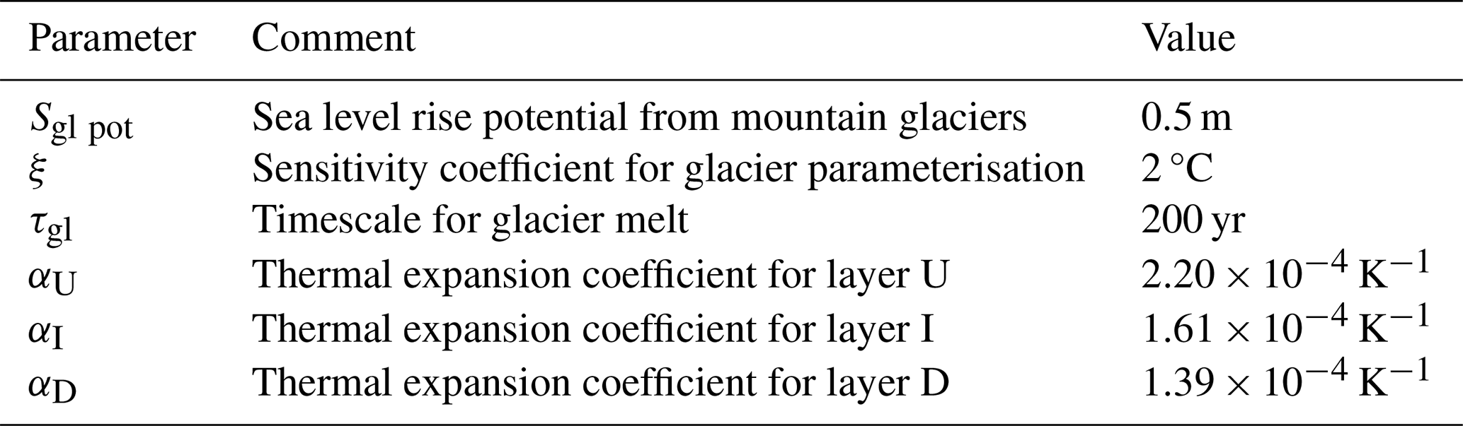
Table 5 Parameter values used for Greenland and Antarctic ice sheets. The values are the same as for SURFER v2.0 (Martínez Montero et al., 2022).

2.4.2 Initial conditions

As in SURFER v2.0, the initial mass of carbon in atmospheric CO₂, M_A(t_PI), is set to have a preindustrial atmospheric CO₂ concentration of 280 ppm. We have

$$\begin{array}{}\text{(106)}& M_{\mathrm{A}}\left(t_{\mathrm{PI}}\right)=\mathrm{280}\times {\mathrm{10}}^{-\mathrm{18}}{m}_{\mathrm{A}}{\stackrel{\mathrm{‾}}{m}}_{\mathrm{C}}=\mathrm{580.27}\mathrm{PgC}.\end{array}$$

The initial mass of carbon in atmospheric CH₄, $M_{\mathrm{A}}^{{\mathrm{CH}}_{\mathrm{4}}}\left(t_{\mathrm{PI}}\right)$, is set to have a preindustrial atmospheric CH₄ concentration of 720 ppb. We have

$$\begin{array}{}\text{(107)}& M_{\mathrm{A}}^{{\mathrm{CH}}_{\mathrm{4}}}\left(t_{\mathrm{PI}}\right)=\mathrm{720}\times {\mathrm{10}}^{-\mathrm{21}}{m}_{\mathrm{A}}{\stackrel{\mathrm{‾}}{m}}_{\mathrm{C}}=\mathrm{1.49}\mathrm{PgC}.\end{array}$$

The initial mass of carbon in land soils and vegetation, M_L(t_PI), is set to 2200 PgC, as in SURFER v2.0. Hence, we have $M_{\mathrm{L}}^{*}\left(t_{\mathrm{PI}}\right)=M_{\mathrm{L}}\left(t_{\mathrm{PI}}\right)=\mathrm{2200}$ PgC. The initial mass of carbon in erodible CaCO₃ sediments, M_S(t_PI), is set to 1600 PgC, following Archer et al. (1998).

For each ocean layer, we have 17 quantities (T, S, K₀, K₁, K₂, K_w, K_b, [H⁺], [H₂CO${}_{\mathrm{3}}^{*}$], [HCO${}_{\mathrm{3}}^{-}$], [CO${}_{\mathrm{3}}^{\mathrm{2}-}$], [OH⁻], [H₃BO₃], [H(BO)${}_{\mathrm{4}}^{-}$], DIC, Alk, and $p_{{\mathrm{CO}}_{\mathrm{2}}}$) that are linked by a nonlinear system of 13 equations (Eqs. 11, 13, 17–22, B1, B2–B5, and B7). Hence, only $\mathrm{17}-\mathrm{13}=\mathrm{4}$ of these quantities may be set independently. Equation (B7) for the pressure dependence of the dissociation constants is not counted because it can be combined with Eqs. (B2)–(B5). For each ocean layer, we will set initial temperature, salinity, alkalinity, and DIC, except for the surface layer where we set [H₂CO${}_{\mathrm{3}}^{*}$] instead of DIC. This is because equilibrium conditions impose a constraint on the H₂CO${}_{\mathrm{3}}^{*}$ mass (and thus [H₂CO${}_{\mathrm{3}}^{*}$]) in the upper layer. Equation (90) gives us

$$\begin{array}{}\text{(108)}& \begin{array}{rl}{M}_{\mathrm{U}}^{\prime }\left(t_{\mathrm{PI}}\right)=& {\displaystyle \frac{W_{\mathrm{U}}{K}_{\mathrm{0}}}{m_{\mathrm{A}}}}{M}_{\mathrm{A}}\left(t_{\mathrm{PI}}\right)+{\displaystyle \frac{W_{\mathrm{U}}}{{\stackrel{\mathrm{‾}}{k}}_{\mathrm{A}\to \mathrm{U}}{m}_{\mathrm{A}}}}\\ & \left(F_{{\mathrm{CaSiO}}_{\mathrm{3}},\mathrm{0}}+F_{{\mathrm{CaCO}}_{\mathrm{3}}\mathrm{0}}\right).\end{array}\end{array}$$

We obtain $M_{\mathrm{U}}^{\prime }\left(t_{\mathrm{PI}}\right)=\mathrm{6.94}$ PgC and [H₂CO${}_{\mathrm{3}}^{*}$]${}_{\mathrm{U}}\left(t_{\mathrm{PI}}\right)=M_{\mathrm{U}}^{\prime }\left(t_{\mathrm{PI}}\right)/\left(W_{\mathrm{U}}{\stackrel{\mathrm{‾}}{m}}_{\mathrm{C}}\right)\times {\mathrm{10}}^{\mathrm{18}}=\mathrm{10.43}$ µmol kg⁻¹. To set the other quantities, we use the GLODAPv2.2016b mapped climatologies (Lauvset et al., 2016), which include climatologies for temperature, salinity, alkalinity, dissolved inorganic carbon, preindustrial dissolved inorganic carbon, and pH among other biogeochemical variables, which were computed based on data gathered between 1972 and 2013. The dissolved inorganic carbon data are normalised to 2002, and the pH is computed based on temperature, alkalinity, and the normalised DIC. We compute the global averages of these data fields over our defined ocean layers by the same averaging method used for computing the thermal expansion coefficients (see Sect. 2.4.1). The values obtained are in Table 6.

Table 6 GLODAPv2.2016b quantities averaged over ocean layers equivalent to those of SURFER.

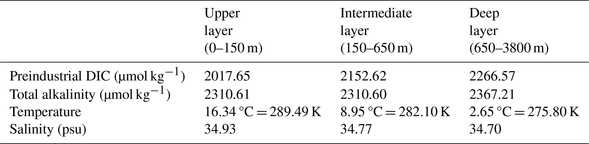
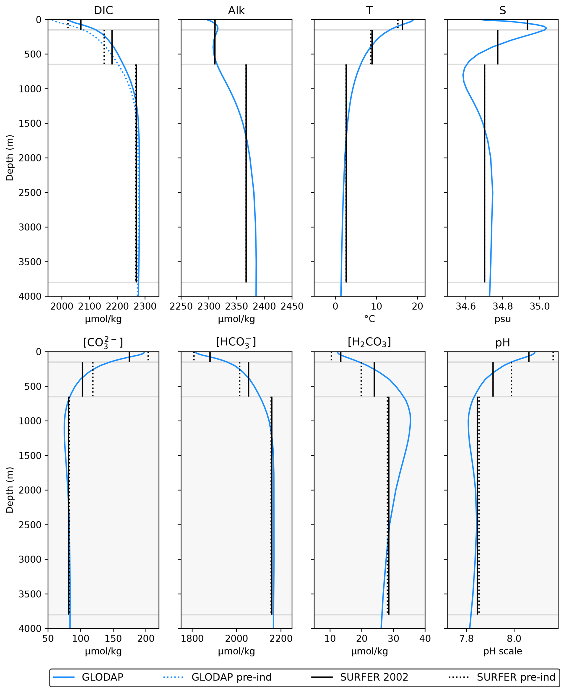
Figure 3 Horizontally averaged quantities from the GLODAPv2.2016b mapped climatologies (Lauvset et al., 2016) compared to initial and simulated values by SURFER v3.0. The carbonate species are not provided in the GLODAP climatologies. We computed their values at each ocean point based on the climatologies of DIC, Alk, temperature, and salinity and then averaged them horizontally. Details for the computation of the carbonate species are in Appendix C.

We set the initial (and constant) salinities S_U, S_I, and S_D of our ocean layers to the computed averages from the GLODAP data. The temperatures of the ocean layers are defined as

$$\begin{array}{}\text{(109)}& T_i\left(t\right)=T_{i,\mathrm{0}}+\mathit{\delta }{T}_i\left(t\right)\mathrm{for}i\in \mathit{\{}\mathrm{U},\mathrm{I},\mathrm{D}\mathit{\}}.\end{array}$$

By definition, the initial conditions for the temperature anomalies δT_i are zero. We set T_i,0 such that T_i(t=2002), obtained from experimental runs, is approximately equal to the temperature average computed from the GLODAP data. We set ${\stackrel{\mathrm{̃}}{Q}}_{\mathrm{U}}\left(t_{\mathrm{PI}}\right)$, ${\stackrel{\mathrm{̃}}{Q}}_{\mathrm{I}}\left(t_{\mathrm{PI}}\right)$, ${\stackrel{\mathrm{̃}}{Q}}_{\mathrm{D}}\left(t_{\mathrm{PI}}\right)$, M_I(t_PI), and M_D(t_PI) based on the computed averages for DIC and Alk, converted to carbon masses with Eqs. (14) and (15). M_U(t_PI) is computed the from the fixed [H₂CO${}_{\mathrm{3}}^{*}$]_U(t_PI), S_U, T_U,0, and Alk_U(t_PI). Details of the computation are provided in Appendix C. We obtain M_U(t_PI)=1344.78 PgC, which corresponds to DIC_U(t_PI)=2022.08 µmol kg⁻¹. This is only 0.22 % off compared to the averaged value for the upper layer obtained from GLODAP. The total dissolved inorganic carbon in the ocean is 37 772 PgC, which is close to the 38 000 PgC estimate from the IPCC (Canadell et al., 2021).

Table 7 Initial conditions for SURFER v3.0. The upper part of the table corresponds to the 17 model variables. The lower part of the table fixes salinity and preindustrial temperature; this is necessary to compute the dissociation constants and the solubility constant of CO₂.

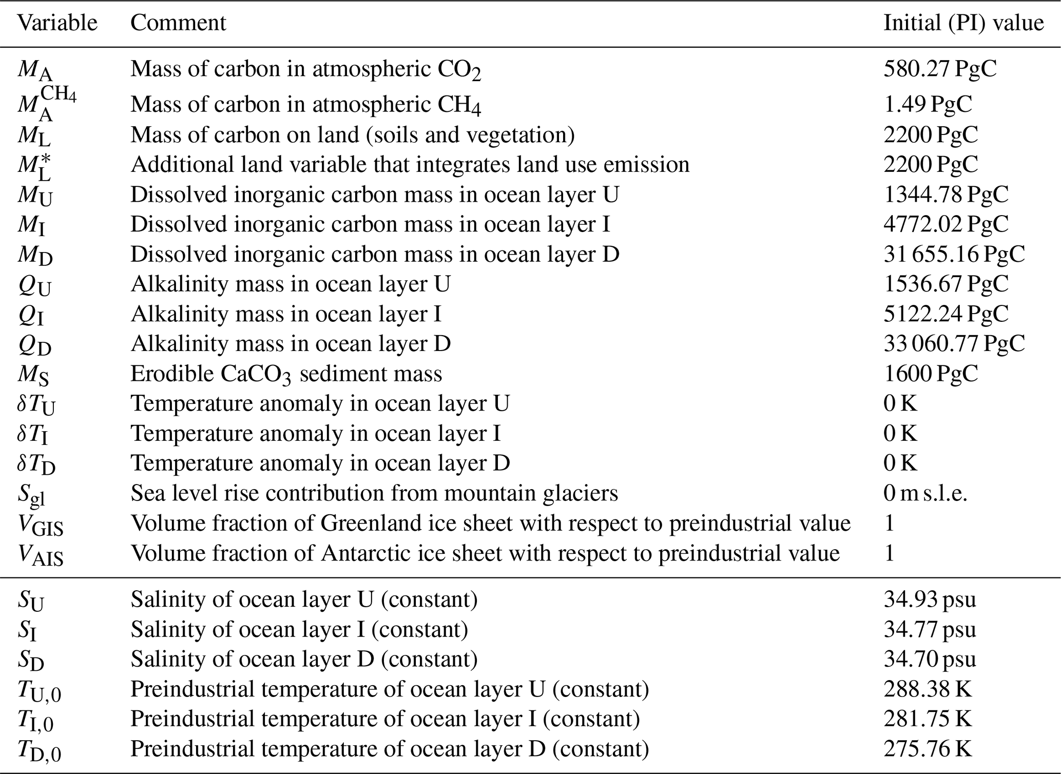
For the sea level rise components, as in SURFER v2.0, we set S_gl(t_PI)=0, V_GIS(t_PI)=1, and V_AI(t_PI)=1. All initial conditions are recapped in Table 7.

In Fig. 3, we compare the horizontally averaged vertical depth profiles of GLODAP to the vertical profiles of SURFER v3.0 for different model quantities. The vertical profiles of SURFER are computed by running the model from 1750 to 2002 forced with historical CH₄ and CO₂ emissions and starting from the initial conditions described above. We observe that the initial conditions chosen produce a model state in 2002 that matches the GLODAP data.

2.5 Numerics

The model is implemented in Python 3.0. using the library solve_ivp with the integration method LSODA. The LSODA method has an automatic stiffness detection and switches accordingly between an Adams and a backward differentiation formula (BDF) method (Petzold, 1983). The local error estimates are kept below $\mathrm{atol}+\mathrm{rtol}\times \mathrm{abs}\left(y\right)$, where atol and rtol are parameters that control the relative and absolute accuracy and where y is a model variable. By default, we set atol to 10⁻³ for the variables $M_{\mathrm{A}}^{{\mathrm{CH}}_{\mathrm{4}}}$ M_S, δT_U, δT_I, δT_D, S_gl, V_GIS, and V_AIS, and we set atol to 10⁻⁶ for the other variables. The reason for this difference is that the variables in the first group can have small or near-zero values, meaning that atol will dominate the local error estimate. If it is too small, the solver takes too many steps and is slow. We set rtol to 10⁻⁶ for all variables. The code is compiled with Numba, and the model runs fast. When forced with CO₂ and CH₄ emissions of a given SSP scenario, runs of 10³ to 10⁶ years typically take around 60 ms on a laptop with an Intel^® Core™ i5-10210U CPU @ 1.60 GHz × 8 processor. The run time is not a linear function of simulated time because the LSODA method uses an adaptive time step.

3 Numerical results and comparisons

In this following section, we test SURFER v3.0 and show that it is an adequate representation of the real climate system. We show that it reproduces well-known dynamics of the carbon cycle, and we compare it with outputs of other models over a large range of timescales.

3.1 Historical period

We show here that SURFER v3.0 is able to reproduce the measured historical CO₂ and CH₄ concentrations and the estimated land and ocean carbon sinks. We perform a historical run by starting SURFER in 1750 with the parameters and initial conditions described in Sect. 2.4. We force the model with fossil and land use emissions of CO₂ and CH₄. Emissions from other greenhouse gases such as nitrous oxide (N₂O), ozone (O₃), halogenated gases, and aerosols are not taken into account. Figures 4 and 5 show the historical CO₂ and CH₄ concentrations simulated by SURFER v3.0 compared to the measurements from Köhler et al. (2017a). SURFER v3.0 is in good agreement with the historical CO₂ observations, with a difference of at most ∼6 ppm, which is better than SURFER v2.0. For methane concentrations, SURFER v3.0 is in relatively good agreement with the historical observations, although it does not capture the apparent stabilisation in the 2000s well. The cause for this stabilisation is not totally clear (Turner et al., 2019). The main hypothesises include a decline in fossil emissions (Chandra et al., 2024) and a shortening of the lifetime of atmospheric CH₄ due to increasing concentrations of the hydroxyl radical caused by changes in emissions of other gases such as N₂O and carbon monoxide (CO) (Skeie et al., 2023). These processes are not modelled in SURFER v3.0, where the atmospheric lifetime of CH₄ is kept constant.

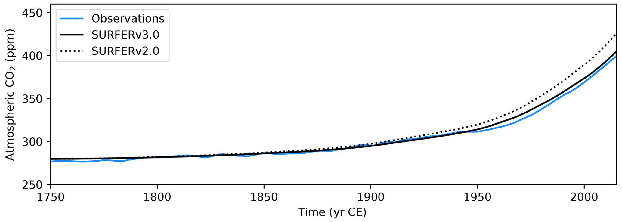
Figure 4 Historical atmospheric CO₂ concentrations. Comparison between (smoothed) observations (Köhler et al., 2017a) and outputs from SURFER v2.0 and SURFER v3.0 when forced with historical emissions.

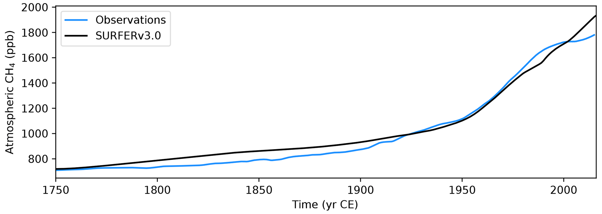
Figure 5 Historical atmospheric CH₄ concentrations. Comparison between (smoothed) observations (Köhler et al., 2017a) and outputs from SURFER v3.0 when forced with historical emissions.

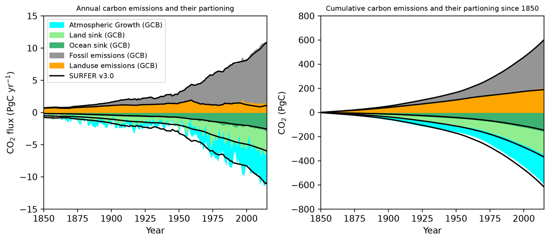
Figure 6 Partitioning of fossil and land use CO₂ emissions in the atmosphere, ocean, and land in SURFER v3.0 compared to estimates from the global carbon budget (GCB) (Friedlingstein et al., 2022).

In Fig. 6, we compare the partitioning of CO₂ emissions in the atmosphere, land, and ocean reservoirs with the estimates from the global carbon budget (GCB) (Friedlingstein et al., 2022). The fossil and land use CO₂ emissions used in SURFER v3.0 up to the year 1990 are the estimates provided by the GCB, and after that, we start using the emission values provided for the SSP scenarios. These are slightly different than the estimates from the GCB (see Appendix A), which explains the small mismatch visible in Fig. 6. In SURFER, we compute the ocean sink as $S_{\mathrm{ocean}}=F_{\mathrm{A}\to \mathrm{U}}-F_{\mathrm{A}\to \mathrm{U}}\left(t_{\mathrm{PI}}\right)$, following the definition of Hauck et al. (2020); the land sink as $S_{\mathrm{land}}=F_{\mathrm{A}\to \mathrm{L}}-F_{\mathrm{A}\to \mathrm{L}}\left(t_{\mathrm{PI}}\right)=F_{\mathrm{A}\to \mathrm{L}}$; and the atmospheric growth as $\frac{\mathrm{d}{M}_{\mathrm{A}}}{\mathrm{d}t}$. These quantities simulated by SURFER v3.0 for the historical period are very close to the estimates from the GCB. For the years 2000 to 2010, the GCB gives a mean estimate of 2.3±0.4 PgC yr⁻¹ for the ocean sink, 2.7±0.5 PgC yr⁻¹ for the land sink, and 4±0.02 PgC yr⁻¹ of atmospheric growth. Values simulated in SURFER v3.0 are 2.16, 3.05, and 3.96 PgC yr⁻¹, respectively, with only the atmospheric growth being just below the GCB estimated range. The cumulative budgets are also very similar: of the total amount of emissions in the period of 1850–2014, the GCB estimates that around 26±5 % are absorbed by the ocean, 31±7 % are absorbed by the land, and 40±1 % stay in the atmosphere, while for SURFER v3.0, those numbers are 24 %, 37 %, and 41 %, respectively. In the GCB, there is a cumulative budget imbalance of 15 PgC for the years 1850–2014, which arises from errors in independent estimates of emissions and sinks, as well as from missing terms in the budget computation. In SURFER v3.0, however, carbon is explicitly conserved, and the budget imbalance (B_im) only results from the definition of the sinks, which do not capture processes such as methane oxidation or changes in carbonate and silicate weathering fluxes. Indeed, we have

$$\begin{array}{}\text{(110)}& {\displaystyle }{B}_{\mathrm{im}}=E_{\mathrm{fossil}}^{{\mathrm{CO}}_{\mathrm{2}}}+E_{\text{land use}}^{{\mathrm{CO}}_{\mathrm{2}}}-\left({\displaystyle \frac{\mathrm{d}{M}_{\mathrm{A}}}{\mathrm{d}t}}+S_{\mathrm{ocean}}+S_{\mathrm{land}}\right)\text{(111)}& {\displaystyle }\begin{array}{rl}=& -V+F_{\mathrm{A}\to \mathrm{U}}\left(t_{\mathrm{PI}}\right)+F_{\mathrm{weathering}}\\ & -\left(F_{{\mathrm{CH}}_{\mathrm{4}},\mathrm{ox}}-E_{\mathrm{natural}}^{{\mathrm{CH}}_{\mathrm{4}}}\right)\end{array}\text{(112)}& {\displaystyle }\begin{array}{rl}=& \left(F_{\mathrm{weathering}}-F_{\mathrm{weathering}}\left(t_{\mathrm{PI}}\right)\right)\\ & -\left(F_{{\mathrm{CH}}_{\mathrm{4}},\mathrm{ox}}-E_{\mathrm{natural}}^{{\mathrm{CH}}_{\mathrm{4}}}\right),\end{array}\end{array}$$

and the cumulative budget imbalance for the years 1850–2014 is −15 PgC, with a contribution of +1 PgC from increased weathering fluxes and −16 PgC from methane oxidation.

3.2 CMIP6 projections

We now compare SURFER v3.0 to the CMIP6 ensemble for the SSP1-2.6 and SSP3-7.0 scenarios. As for the historical runs in Sect. 3.1, SURFER v3.0 is forced with CO₂ and CH₄ fossil and land use emissions but no other greenhouse gases or aerosols. Runs are started in 1750, and the results for atmospheric CO₂, temperature, surface ocean pH, ocean carbon uptake, and land carbon uptake are plotted in Fig. 7. Additionally, we compare these with outputs from SURFER v2.0 forced with the total CO₂ emissions and run with the parameters and initial conditions described in Martínez Montero et al. (2022).

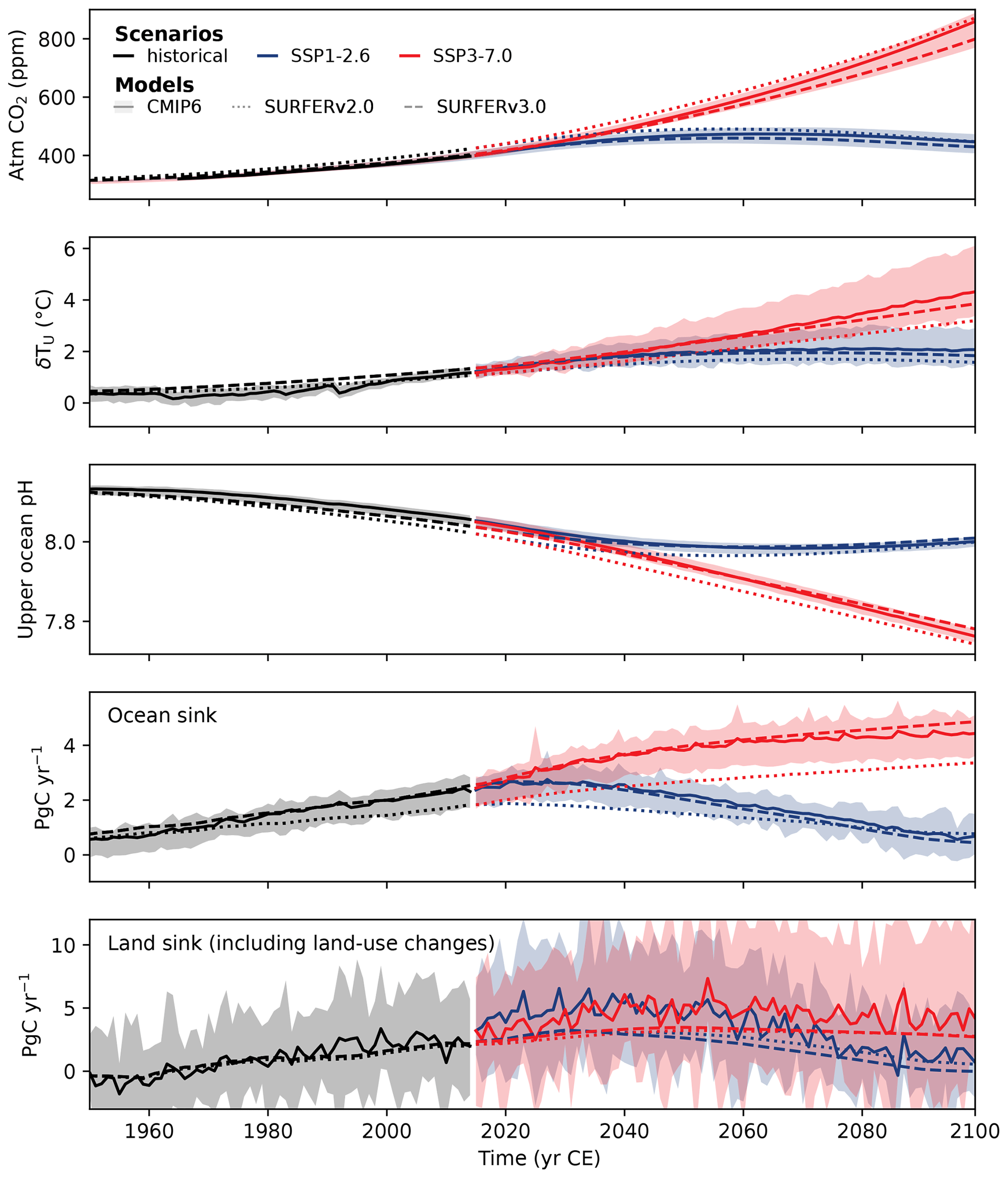
Figure 7 Comparison between SURFER v3.0, SURFER v2.0, and the CMIP6 model ensemble mean for the historical period (1750–2014) and the near future (2015–2100) under the SSP1-2.6 and SSP3-7.0 scenarios. The CMIP6 data are from concentration-driven runs, except the atmospheric CO₂, which comes from emission-driven runs. The ocean sink is computed in SURFER as $F_{\mathrm{A}\to \mathrm{U}}-F_{\mathrm{A}\to \mathrm{U}}\left(t_{\mathrm{PI}}\right)$. The land sink is taken here as the net biome productivity (NBP), which includes land use fluxes. In SURFER, it is computed as $F_{\mathrm{A}\to \mathrm{U}}-E_{\text{land use}}^{{\mathrm{CO}}_{\mathrm{2}}}-E_{\text{land use}}^{{\mathrm{CH}}_{\mathrm{4}}}$.

As already shown in Fig. 4, SURFER v3.0 reproduces the historical CO₂well, and for the SSP scenario projections, it falls within the lower range of the CMIP6 model ensemble. SURFER v3.0 can simulate a global mean temperature anomaly that generally remains within the CMIP6 range, considering only the effects of CO₂ and methane. This is because the contributions from the other major drivers of temperature changes such as nitrous oxide (N₂O), ozone (O₃), halogenated gases, and aerosols approximately cancel each other out (Forster et al., 2021, see Fig. 7.8). However, between 1960 and 2015, the cooling effect of aerosols from anthropogenic and volcanic sources was likely more significant, and without accounting for this, SURFER v3.0 simulates temperatures slightly above the CMIP6 range.

Surface pH simulated by SURFER v3.0 generally aligns with the CMIP6 range for both the historical period and SSP projections, an improvement over SURFER v2.0, which showed too rapid ocean acidification. This improvement is primarily due to the addition of a new intermediate layer in SURFER v3.0, which facilitates faster carbon transfer out of the upper-ocean layer, thereby slowing surface acidification. This enhanced carbon transfer to intermediate- and deep-ocean layers also allows the ocean to absorb CO₂ more efficiently. As a result, the ocean carbon uptake in SURFER v3.0 now falls within the CMIP6 model range. The land carbon uptakes in SURFER v3.0 and v2.0 are very similar, and both are in the range of the CMIP6 models, which is quite large and demonstrates a higher uncertainty.

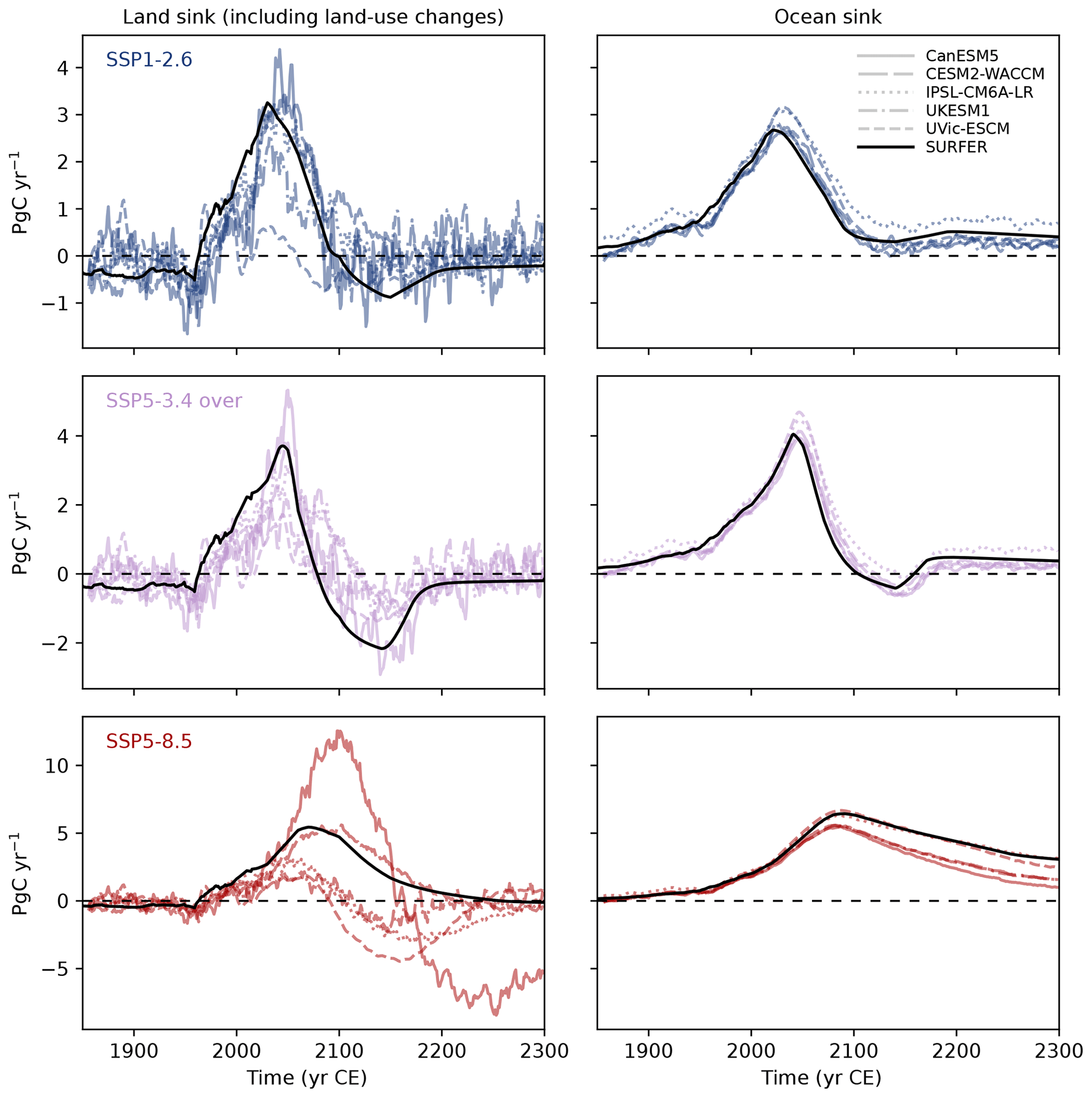
Figure 8 Comparison of atmosphere-to-ocean and atmosphere-to-land carbon fluxes as simulated by SURFER v3.0 and CMIP6 models for the historical period (1750–2014) and the future (2015–2300) under the SSP1-2.6, SSP5-3.4 over, and SSP5-8.5 scenarios. The ocean sink is computed in SURFER as $F_{\mathrm{A}\to \mathrm{U}}-F_{\mathrm{A}\to \mathrm{U}}\left(t_{\mathrm{PI}}\right)$. The land sink is taken here as the net biome productivity (NBP), which includes land use fluxes. In SURFER, it is computed as $F_{\mathrm{A}\to \mathrm{U}}-E_{\text{land use}}^{{\mathrm{CO}}_{\mathrm{2}}}-E_{\text{land use}}^{{\mathrm{CH}}_{\mathrm{4}}}$.

In Fig. 8, we compare the land and ocean sinks of SURFER to four CMIP6 models and one EMIC that have been run to the year 2300 under the SSP1-2.6, SSP3-4.3, and SSP5-8.5 scenarios. We observe that SURFER v3.0 remains within the range of CMIP6-class models even over these longer timescales. For all three scenarios, the land sink is expected to become negative at some point, indicating that the land reservoir will release some of the carbon it had previously absorbed (Canadell et al., 2021; Tokarska et al., 2016; Zickfeld et al., 2013). For the SSP1-2.6 and SSP-3.4 scenarios, this negative land sink in CMIP6 models is attributed to the land carbon–concentration feedback: as CO₂ concentrations decrease after strong negative emissions, vegetation releases carbon. For the SSP5-8.5 scenario, the negative land sink is instead due to a stronger land carbon–climate feedback, where warming leads to a release of CO₂ from the land reservoir, for example, through increased decomposition rates (Tokarska et al., 2016). In SURFER, the parameterisation of the atmosphere-to-land flux (F_A→L) depends on the atmospheric CO₂ concentration (M_A) but not on temperature, effectively including only a carbon–concentration feedback. This explains why, for the SSP5-8.5 scenario, the land sink in SURFER only becomes slightly negative around 2250, when the atmospheric CO₂ concentrations begin to decline. Despite this, the land sink from SURFER remains mostly in the range of the other models, which is quite large and reflects the large uncertainty in processes related to the terrestrial biosphere.

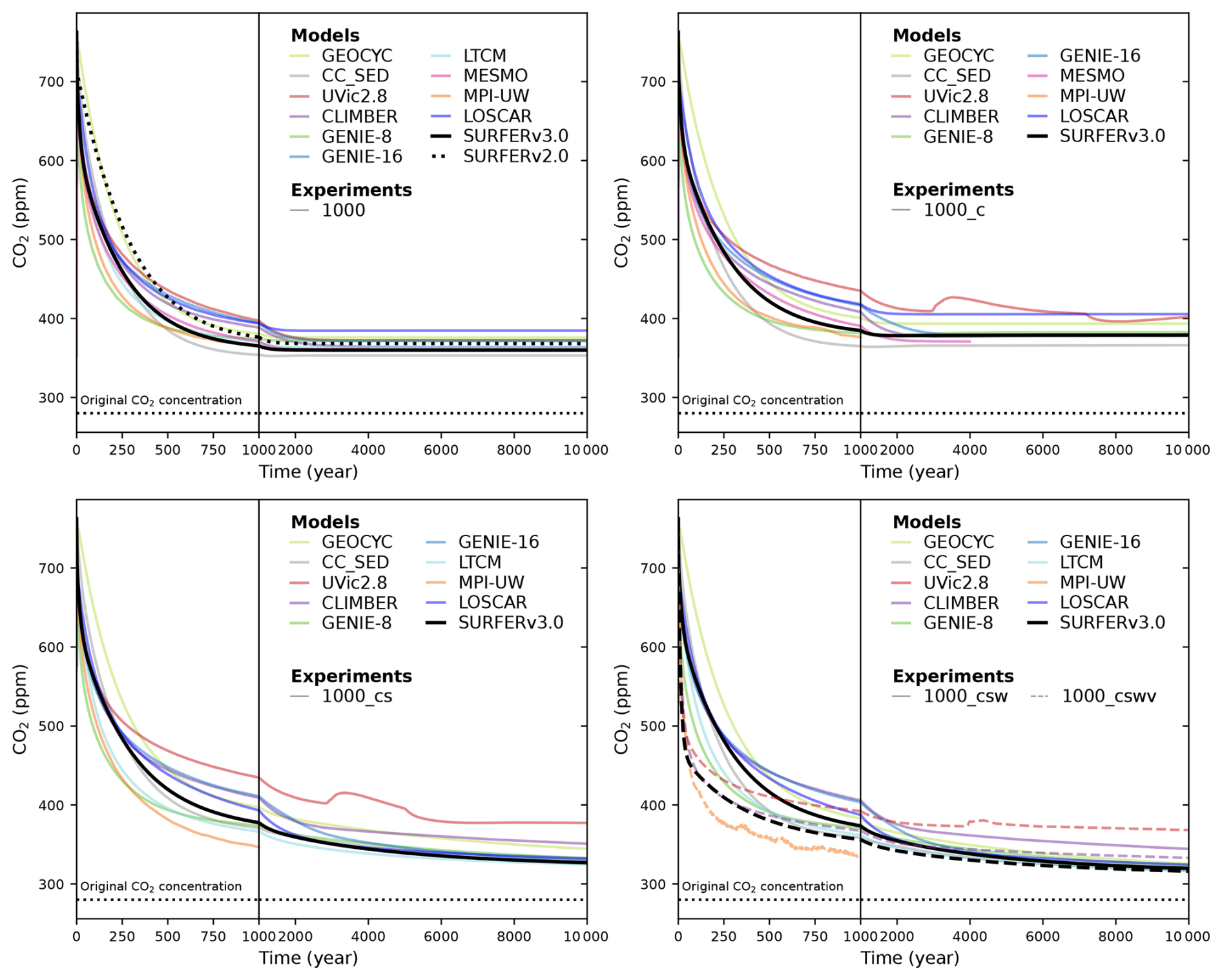
Figure 9 Atmospheric CO₂ simulated by different models and SURFER v3.0 after a 1000 PgC emission pulse for the LTMIP experiments. The five experiments are the baseline (ocean only) experiment; the climate (C); the climate and sediments (CS); the climate, sediments, and weathering (CSW); and the climate, sediments, weathering, and vegetation (CSWV) experiments. We have added the results of the LOSCAR model (Zeebe, 2012), which was not part of the original LTMIP publication (Archer et al., 2009).

3.3 LTMIP

In the previous sections, we have seen that SURFER v3.0 can reproduce the historical record and outputs from CMIP6-class models for projections up to 2300. Here, we focus on longer timescales and compare SURFER v3.0 with results from the Long-Tail Model Intercomparison Project (LTMIP; Archer et al., 2009). In these experiments, several models were used to assess the CO₂ draw-down from the atmosphere for 10 000 years after emissions pulses of 1000 and 5000 PgC. For each emission pulse, five experiments are performed with different physical processes progressively included to assess their impact on atmospheric CO₂ uptake. These experiences are named with a combination of letters indicating the processes included: climate feedbacks (C), sediments (S), weathering (W), and vegetation (V). We reproduce these experiments with SURFER v3.0 by successively reducing the number of active processes. For, the CSWV experiment, we use the standard version of SURFER v3.0. For the CSW experiment, we set $k_{\mathrm{A}\to \mathrm{L}}=\mathrm{0}$ so that vegetation is kept constant and has no influence on carbon uptake ($F_{\mathrm{A}\to \mathrm{L}}=\mathrm{0}$). For the CS experiment, we additionally keep the weathering fluxes $F_{{\mathrm{CaCO}}_{\mathrm{3}}}$ and $F_{{\mathrm{CaSiO}}_{\mathrm{3}}}$ constant and equal to their preindustrial values, thus eliminating weathering feedbacks. For the C experiment, we further keep the accumulation and burial fluxes constant and equal to their preindustrial values, thus effectively eliminating interactions with the sediments. Finally for the baseline experiment, on top of all the modifications described above, we keep the solubility and dissociation constants constant. In this last case, SURFER v3.0 is very similar to SURFER v2.0.

Results for these five experiments are shown in Fig. 9 for the 1000 PgC pulse and in Fig. 10 for the 5000 PgC pulse. Overall, SURFER v3.0 falls within the range of other models, except in the following cases: the 5000 PgC baseline experiment after 1000 years, the 5000 PgC C experiment between the years 1000 and 5000, and the CSWV experiments after the year 1000, where SURFER v3.0 simulates slightly lower atmospheric CO₂ levels than the other models. For the baseline experiment, SURFER v2.0 does not absorb CO₂ from the atmosphere fast enough in the first thousand years after the emission pulse. As already mentioned, this is improved in SURFER v3.0 thanks to the addition of a third oceanic layer at intermediate depth.

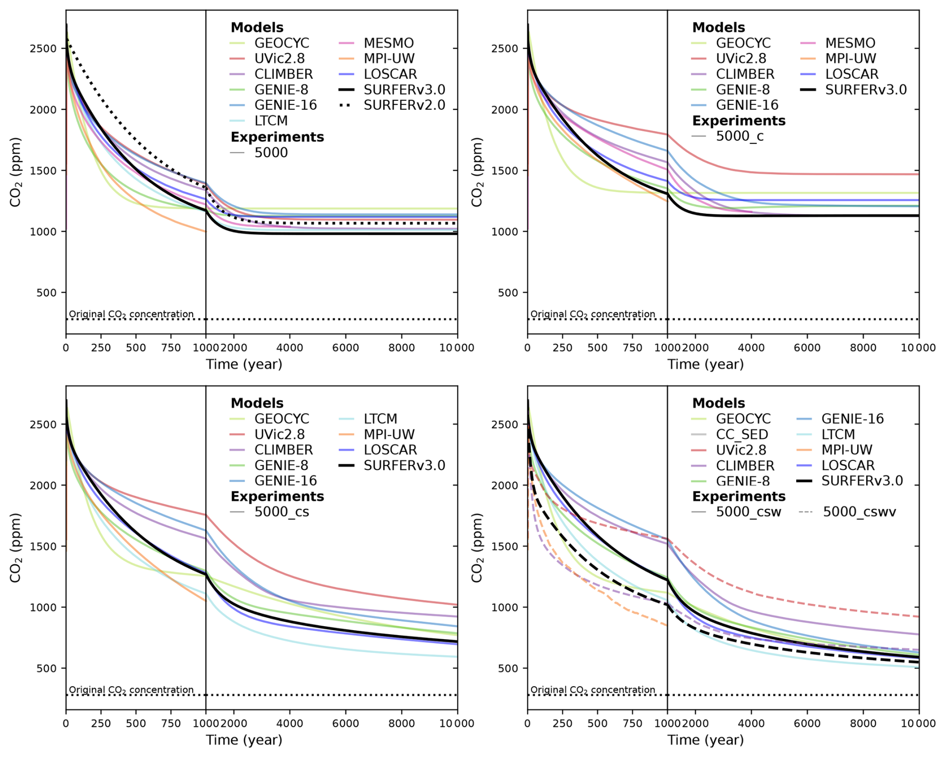
Figure 10 Atmospheric CO₂ simulated by different models and SURFER v3.0 after a 5000 PgC emission pulse for the LTMIP experiments. The five experiments are the baseline (ocean only) experiment; the climate (C); the climate and sediments (CS); the climate, sediments, and weathering (CSW); and the climate, sediments, weathering, and vegetation (CSWV) experiments. We have added the results of the LOSCAR model (Zeebe, 2012), which was not part of the original LTMIP publication (Archer et al., 2009).

We can define and quantify the climate, sediment, weathering, and vegetation feedbacks by taking the difference in simulated atmospheric CO₂ between consecutive experiments (C − baseline, CS − C, CSW − CS, and CSWV − CSW). The results are plotted in Fig. 11 for the 1000 PgC pulse and in Fig. 12 for the 5000 PgC pulse. Not all experiments were performed for each model, so feedbacks cannot always be computed. All experiments are only available for CLIMBER and SURFER v3.0. Overall, the feedbacks in SURFER v3.0 fall within the range of the other models, demonstrating that the associated processes are reasonably well simulated by SURFER. For the 5000 PgC pulse experiments, the climate feedback in SURFER v3.0 is very similar to the LOSCAR and GEOCYC models but quite different from the other models. This is probably explained by SURFER V3.0, as well as LOSCAR and GEOCYC, all missing dynamic ocean circulation and hence feedbacks associated with temperature-induced circulation changes. The sediment feedback in SURFER v3.0 for the 1000 PgC pulse is in the higher range (more negative) of the other models, which is consistent with the dissolution flux being generally larger (accumulation more negative) than in the other models (see Fig. 13). For the 5000 PgC pulse, the sediment feedback in SURFER v3.0 is in the mid-to-lower range of the other models, despite the dissolution flux still being in the higher range. In general, other than oceanic invasion, vegetation has the biggest impact on CO₂ uptake before the year 1000, while sediments have the biggest impact between the years 1000 and 10 000.

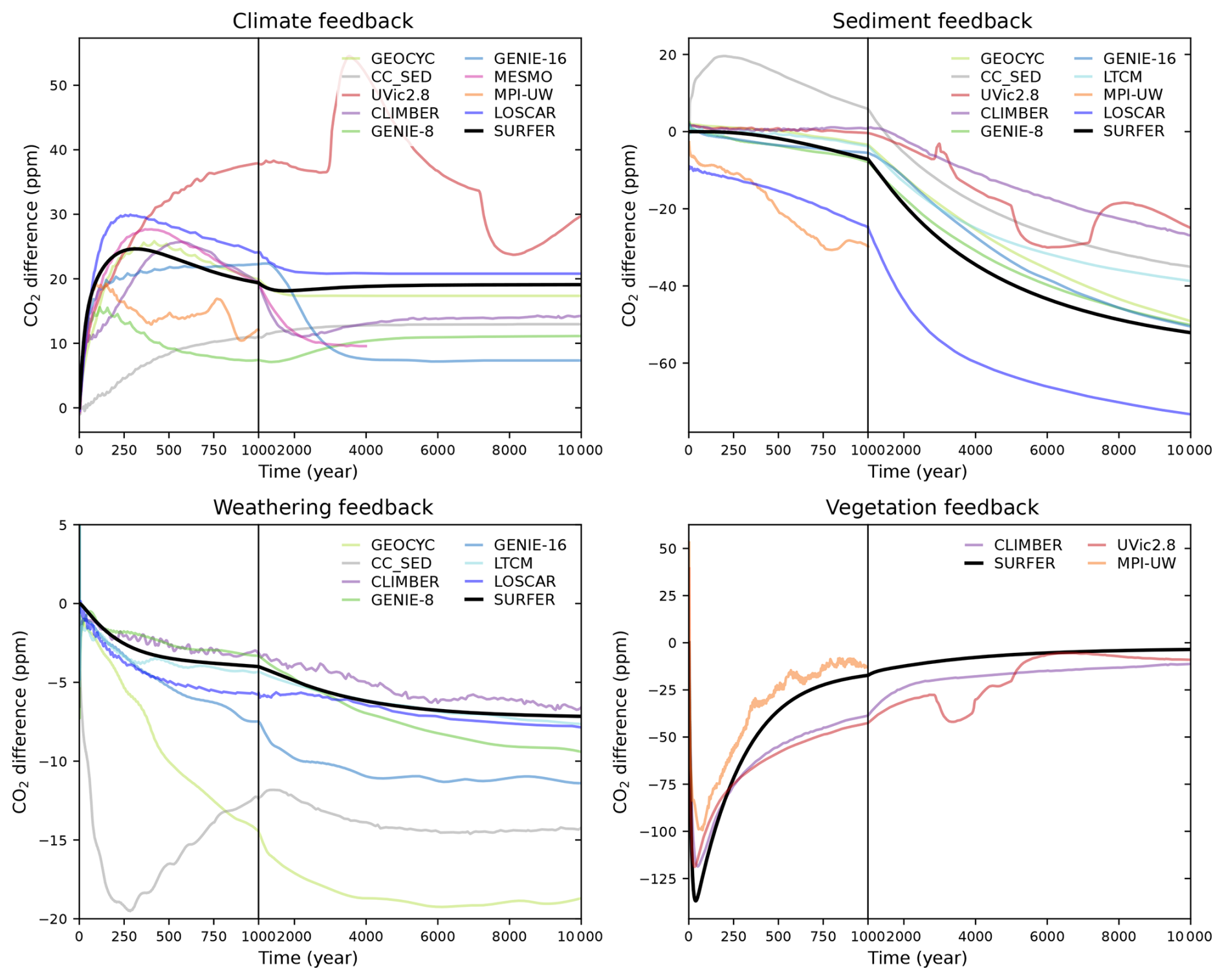
Figure 11 Impacts of the climate, sediments, weathering, and vegetation feedbacks on the atmospheric CO₂ concentration after a 1000 PgC emission pulse. Here, a feedback is defined as the difference in CO₂ concentration resulting from the addition of the associated process.

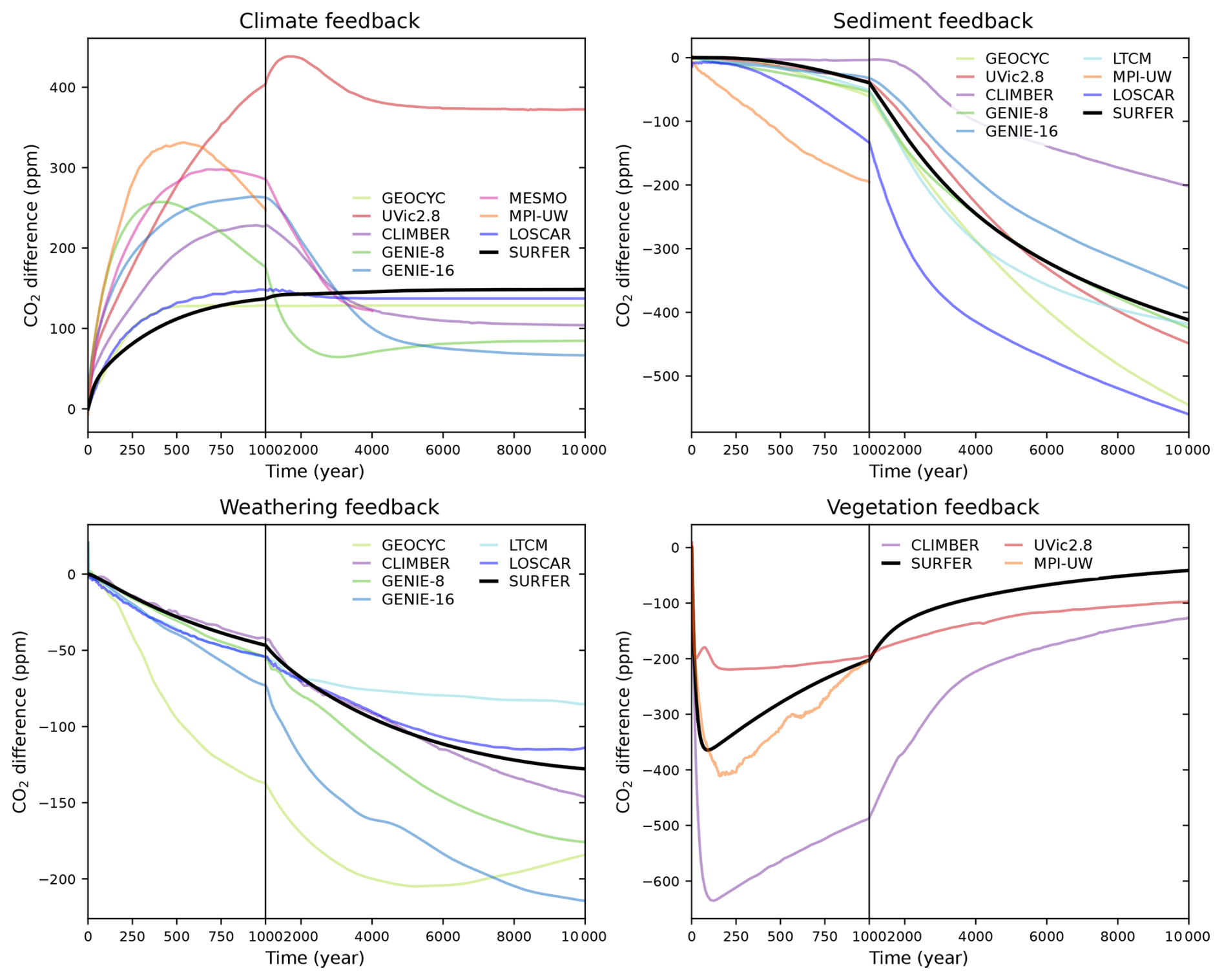
Figure 12 Impacts of the climate, sediments, weathering, and vegetation feedbacks on the atmospheric CO₂ concentration after a 5000 PgC emission pulse. Here, a feedback is defined as the difference in CO₂ concentration resulting from the addition of the associated process.

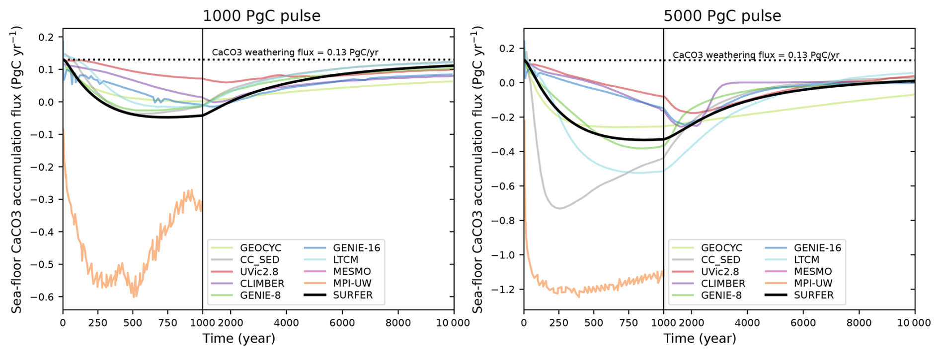
Figure 13 CaCO₃ accumulation fluxes in sediments for the different models. Negative values indicate net dissolution of CaCO₃.

3.4 cGENIE

Only a few models of intermediate complexity have been run for 100 kyr or more to investigate the carbon cycle's response to (anthropogenic) CO₂ emissions. Some examples include cGENIE (Colbourn et al., 2013, 2015; Lord et al., 2016) and CLIMBER-X (Kaufhold et al., 2024). Here, we compare SURFER v3.0 with the 1 Myr runs performed with the cGENIE model of intermediate complexity (Lord et al., 2016). This model comprises a 2D energy–moisture balance atmosphere, a 3D frictional geostrophic ocean circulation model, and a representation of the global carbon cycle, with ocean cycling of DIC, alkalinity, and a nutrient (PO₄); CaCO₃ marine sediments; and terrestrial weathering (Edwards and Marsh, 2005; Ridgwell et al., 2007; Ridgwell and Hargreaves, 2007; Colbourn et al., 2013). For the runs presented here (Lord et al., 2016), cGENIE was used without the terrestrial biosphere module and its associated carbon fluxes. The model had eight ocean levels, with the surface layer being 175 m deep, comparable to the surface layer in SURFER v3.0.

We perform equivalent runs in SURFER v3.0 with $k_{\mathrm{A}\to \mathrm{L}}=\mathrm{0}$ to neglect the role of vegetation. Results are plotted in Figs. 14 and 15 for atmospheric CO₂, global mean temperature, ocean surface pH, ocean surface calcite saturation state, and CaCO₃ content in sediments. Ocean surface calcite saturation state, Ω_U, is defined as

$$\begin{array}{}\text{(113)}& {\mathrm{\Omega }}_{\mathrm{U}}={\displaystyle \frac{{\left[{\mathrm{CO}}_{\mathrm{3}}^{\mathrm{2}-}\right]}_{\mathrm{U}}{\left[{\mathrm{Ca}}^{\mathrm{2}+}\right]}_{\mathrm{U}}}{K_{\mathrm{sp}}^{{\mathrm{CaCO}}_{\mathrm{3}}}}}.\end{array}$$

The solubility product $K_{\mathrm{sp}}^{{\mathrm{CaCO}}_{\mathrm{3}}}=\left[{\mathrm{CO}}_{\mathrm{3}}^{\mathrm{2}-}{]}_{\mathrm{sat}}\right[{\mathrm{Ca}}^{\mathrm{2}+}{]}_{\mathrm{sat}}$ depends on salinity, temperature, and pressure (Mucci, 1983; Millero, 1995). For the computation of Ω_U, we use the parameterisations of $K_{\mathrm{sp}}^{{\mathrm{CaCO}}_{\mathrm{3}}}$ described in Appendix B, and we assume that [Ca²⁺]_U is constant and equal to 0.01028 mol kg⁻¹ (Sarmiento and Gruber, 2006).

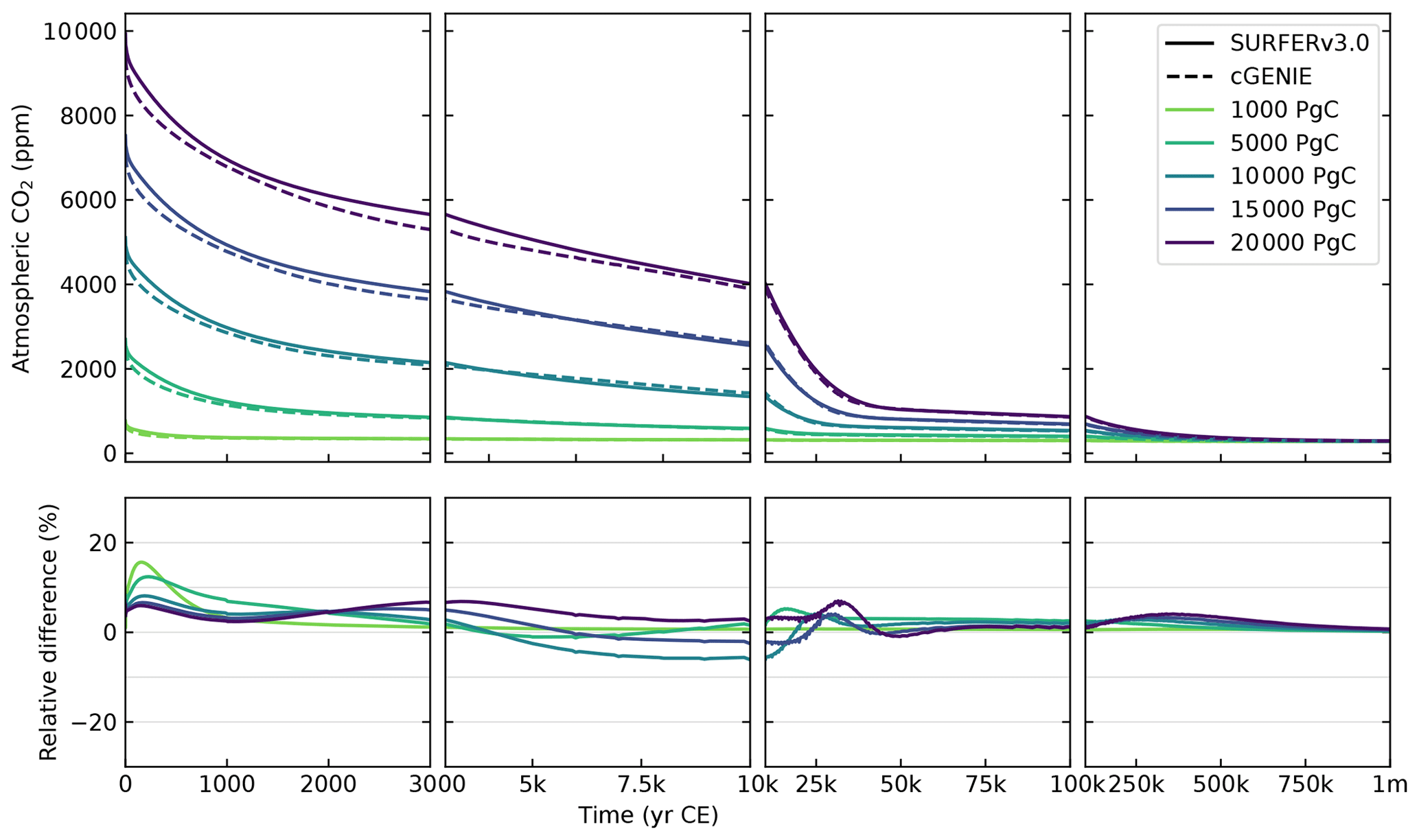
Figure 14 Atmospheric CO₂ concentrations simulated by cGENIE and SURFER v3.0 after emissions pulses of different sizes. The bottom panels show the relative differences between SURFER v3.0 and cGENIE.

Overall, SURFER v3.0 reproduces the behaviour of cGENIE well. For all emission pulses, the relative difference in simulated atmospheric CO₂ with cGENIE does not exceed 18 %, is lower than 8 % after 1000 years, and is below 5 % after 50 kyr. These are smaller differences than those between models for the LTMIP experiments (see Figs. 9 and 10). This good agreement for millennial and longer timescales was expected, as SURFER v3.0 was qualitatively tuned to cGENIE's long-term atmospheric CO₂ output. The agreement in ocean surface pH is also very strong, with absolute differences below 0.06 pH units after 5 years, below 0.04 pH units after 1000 years, and below 0.02 pH units after 50 kyr, corresponding to a relative difference below 1 % after 5 years for all emissions pulses. Because the carbon exchanges between the atmosphere and the surface ocean reach equilibrium relatively fast, the good agreement for ocean surface pH directly results from the good agreement for atmospheric CO₂ concentrations. Regarding temperatures, peak warming occurs later in SURFER v3.0 than in cGENIE, primarily because SURFER only models ocean temperatures, leading to slower global warming compared to cGENIE, which also accounts for the thermal balance of the continents.

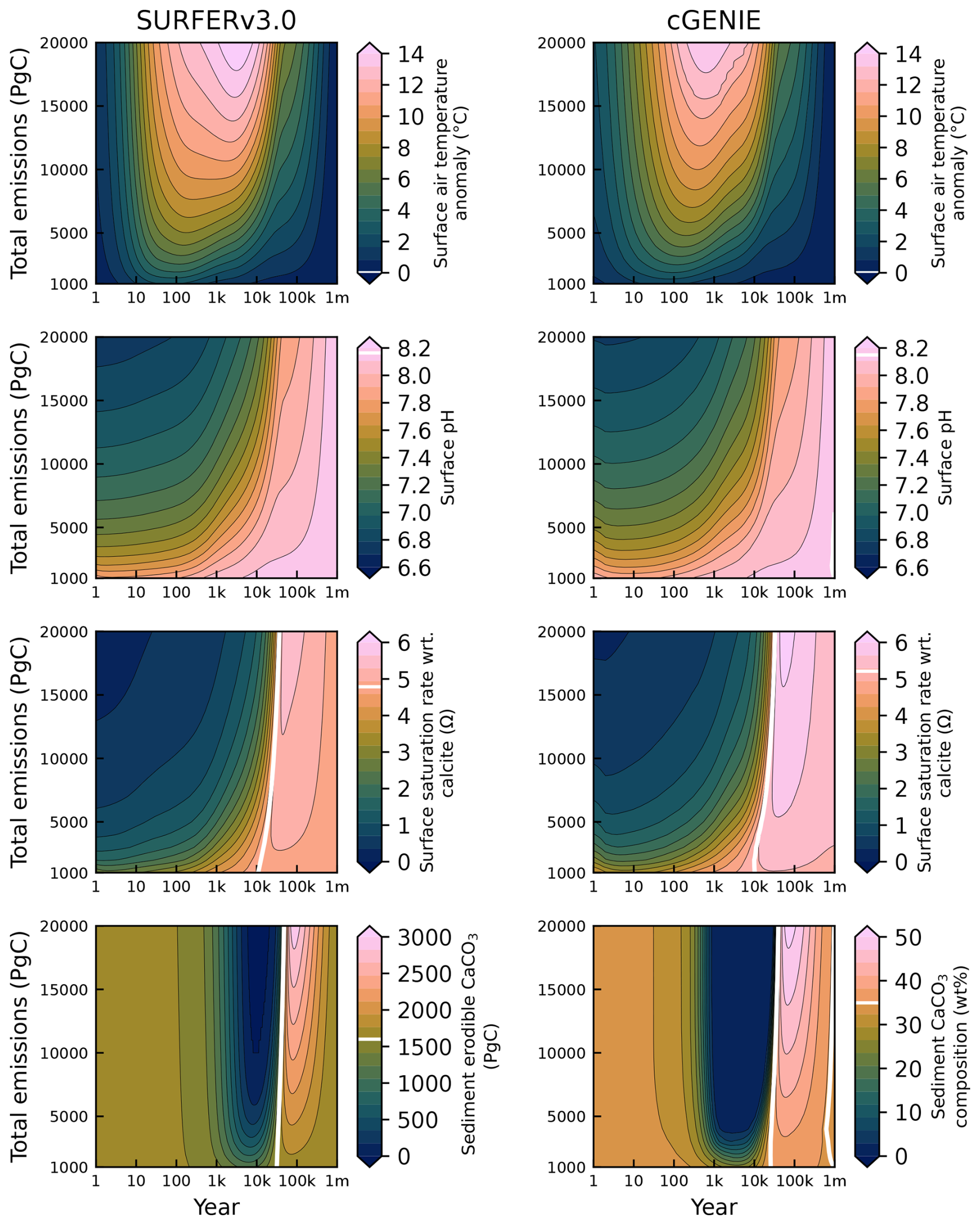
Figure 15 Global mean temperature anomaly, surface ocean pH, surface ocean saturation state with respect to calcite, and CaCO₃ sediment content in SURFER v3.0 and cGENIE after emissions pulses ranging from 1000 to 20 000 PgC. White lines indicate the preindustrial values used in each model. Note that SURFER v3.0 and cGENIE use different units for the CaCO₃ sediment content. SURFER uses the total erodible CaCO₃ mass, while cGENIE uses the mean dry weight fraction (mass of CaCO₃ divided by the mass of CaCO₃ and nonerodible material in sediments). Although these two quantities are strongly correlated, they do not necessarily depend linearly on one another, complicating direct comparisons.

After 1 Myr, the state is almost back to equilibrium in SURFER v3.0, with atmospheric CO₂ concentrations ranging from 280.68 ppm for the 1000 PgC emission pulse to 292.08 ppm for the 20 000 PgC pulse. Carbon is removed from the atmosphere through a range of processes. First, atmospheric CO₂ dissolves in the upper-ocean layer following the reaction

$$\begin{array}{}\text{(1)}& {\mathrm{CO}}_{\mathrm{2}}+{\mathrm{H}}_{\mathrm{2}}\mathrm{O}+{\mathrm{CO}}_{\mathrm{3}}^{\mathrm{2}-}\rightleftharpoons \mathrm{2}{\mathrm{HCO}}_{\mathrm{3}}^{-},\end{array}$$

which is equivalent to Reactions R1–R3. This causes a decrease in ocean surface pH (acidification) and consumes CO${}_{\mathrm{3}}^{\mathrm{2}-}$, which results in a decrease in the surface calcite saturation state. Both these effects are observable in SURFER v3.0 and cGENIE. On centennial to millennial timescales, the CO${}_{\mathrm{3}}^{\mathrm{2}-}$ anomaly mixes into the ocean interior and deep waters become less saturated, causing an increase in the dissolution of deep-sea CaCO₃ sediments and a release of carbonate ions. Some of these carbonate ions can then react with CO₂ (Reaction 1), leading to further oceanic CO₂ uptake. This process is called sea floor neutralisation, as it is the dissolution of previously deposited deep-sea sediments that allows the neutralisation of atmospheric CO₂ (Archer et al., 1997, 1998). Moreover, the increased dissolution of CaCO₃ sediments compared to the preindustrial state creates an imbalance between the alkalinity input to the ocean by weathering and the alkalinity output by accumulation. This replenishes the ocean CO${}_{\mathrm{3}}^{\mathrm{2}-}$ concentration and the erodible CaCO₃ sediment stock while leading to further uptake of atmospheric CO₂. This second process is called terrestrial neutralisation, as it is the (imbalanced) dissolution of carbonate and silicate rocks on land that neutralise the atmospheric CO₂ (Archer et al., 1997, 1998; Ridgwell and Hargreaves, 2007). We observe an overshoot in the surface calcite saturation state and deep-sea ocean sediment content compared to the preindustrial situation in both SURFER v3.0 and cGENIE because of increased weathering rates due to warming. The extra CaCO₃ in the sediments will eventually be buried, leading to a permanent transfer of carbon to the geological reservoir.

4 Sea level rise and the importance of long-timescale processes

So far, we have focused primarily on the carbon cycle, as the additions to SURFER v3.0 are related to it. In this section, we examine sea level rise (SLR), which is computed as the sum of four contributions: thermosteric sea level rise (thermal expansion), glaciers, Greenland, and Antarctica. The parameterisation for thermosteric sea level rise in SURFER v3.0 is essentially the same as in SURFERv2.0, with the key differences being the use of three ocean layers instead of two and the use of new thermal expansion coefficients. In Sect. 4.1, we verify that these changes still provide a reasonable approximation of thermosteric SLR. The parameterisations for glaciers, Greenland, and Antarctica remain unchanged between SURFER v2.0 and SURFER v3.0, so any difference in SLR contributions under a given forcing scenario results only from differences in simulated temperatures. We investigate the SLR contribution from the ice sheets in Sect. 4.2.

4.1 Thermosteric sea level rise and ocean heat content

Heat transfer in the SURFER v3.0 ocean is controlled by the parameters γ_U→I and γ_I→D. The heat accumulated in ocean layers, along with the corresponding temperature increases, determines thermosteric sea level rise. To ensure that our chosen values for γ_U→I, γ_I→D, and the thermal expansion coefficients are reasonable, we compare the ocean heat content and thermosteric sea level rise in SURFER v3.0 with IPCC estimates for 1971–2018 (Fig. 16).

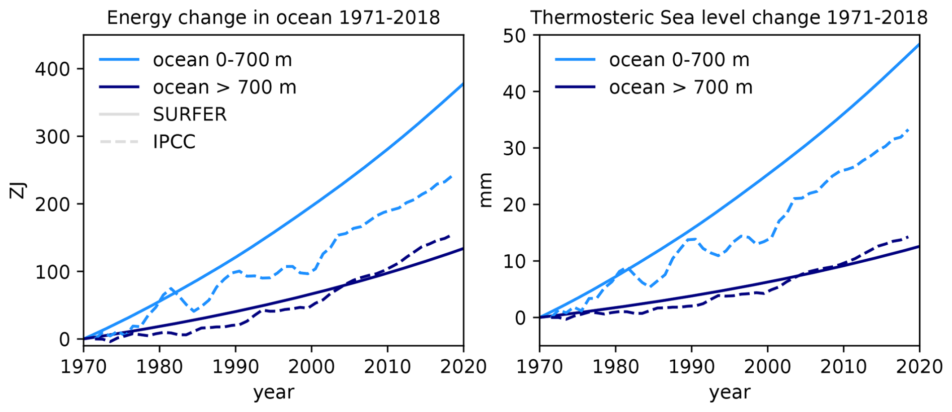
Figure 16 The ocean heat content and thermosteric sea level changes between the years 1971 and 2018, as estimated by the IPCC (Fox-Kemper et al., 2021) and simulated by SURFER v3.0.

SURFER v3.0 simulates significantly higher ocean heat content above 700 m (layers U and I) than the IPCC estimates, resulting in a larger thermosteric sea level rise. This discrepancy arises for two reasons. First, in SURFER, all energy imbalance is absorbed by the ocean, with no energy allocated to warming the land and atmosphere or for melting glaciers and ice sheets. Consequently, the ocean warms more than it should. Second, and more importantly, SURFER v3.0 does not account for faster and larger land temperature increases, which cause the global mean temperature rise to be higher when averaged over land and oceans. In other words, SURFER assumes that the global mean temperature is equivalent to the ocean's mean surface temperature. As a result, SURFER needs more energy to reproduce the observed global mean temperatures and overestimates surface ocean temperatures. For the ocean below 700 m (layer D in SURFER), the ocean heat content and the thermosteric sea level rise simulated by SURFER v3.0 match the IPCC estimates quite well. This indicates that the oceanic heat transport at depth is a little too slow, which compensates for the ocean receiving more energy than it should.

We also check that our parameterisation for thermosteric sea level rise is valid on longer timescales. In Fig. 17, we compare outputs from the intermediate complexity model UVic, versions 2.8 and 2.9 (Eby et al., 2009; Clark et al., 2016), to outputs from SURFER v2.0 and SURFER v3.0. The UVic 2.8 and UVic 2.9 models both include a sediment module and have equilibrium climate sensitivities around 3.5 °C, the same as in SURFER. Emission scenarios used to force the models follow historical estimates of CO₂ emissions up to the year 2000. Following this, cumulative emissions of either 1280 or 3840 PgC are added between the years 2000 and 2300. For more details on the experimental setup, see Clark et al. (2016).

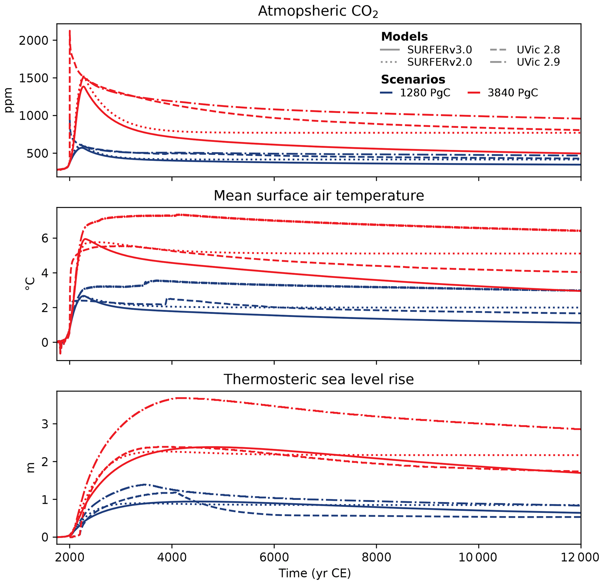
Figure 17 Atmospheric CO₂, surface temperature, and thermosteric sea level rise simulated by SURFER v3.0, SURFER v2.0, and two versions of the UVic model of intermediate complexity for two emission scenarios: 1280 PgC (blue) and 3840 PgC (red).

SURFER v3.0 has faster and larger atmospheric CO₂ uptake than both UVic 2.8 and UVic 2.9. This is consistent with the LTMIP experiments (Figs. 9 and 10), where UVic 2.8 was already the model with the smallest CO₂ uptake after 10 000 years for the CSWV experiments. UVic 2.9 has even slower CO₂ uptake than UVic 2.8 due to the difference in the sediments representation (Clark et al., 2016). For SURFER v2.0, the atmospheric CO₂ concentration reaches equilibrium after ∼4000 years since it only takes into account the process of ocean CO₂ invasion. These differences in atmospheric CO₂ concentrations lead to relatively large differences in global mean surface temperatures. Nevertheless, the thermosteric SLR is comparable in all models, except for in UVic 2.9 under the 3840 PgC scenario, where it is larger than in the other models. The thermosteric SLR from SURFER v3.0 is close to the one from UVic 2.8 for both scenarios, even though the simulated temperature is lower in SURFER v3.0. This is again a consequence of SURFER not simulating land temperatures. The global mean ocean temperature increase in UVic 2.8 is smaller than its global mean temperature increase and probably comparable to the mean ocean temperature observed in SURFER v3.0. SURFER v3.0 and SURFER v2.0 also have comparable thermosteric SLR despite SURFER v2.0 simulating a larger temperature increase. This is because the ocean in SURFER v3.0 is deeper than in SURFER v2.0 (3800 m deep vs. 3150 m deep) and thus has more potential for expansion.

4.2 Ice sheets

In SURFER v2.0, atmospheric CO₂ concentrations, and hence temperatures, stabilise a few thousand years after the end of emissions. In SURFER v3.0, thanks to new processes added in the carbon cycle, CO₂ draw-down from the atmosphere continues until a return to preindustrial conditions, leading to lower temperatures than in SURFER v2.0 on millennial and longer timescales. Since ice sheets respond on the millennial timescale, we expect these differences to have a significant impact on their melting. To test this, we force both SURFER v3.0 and SURFER v2.0 with the CO₂ emissions from five SSP scenarios (SSP1-2.6, SSP2-4.5, SSP4-6.0, SSP3-7.0, SSP5-8.5), which cover a range of possible futures. Simulations last for 500 kyr, and the results are plotted in Fig. 18.

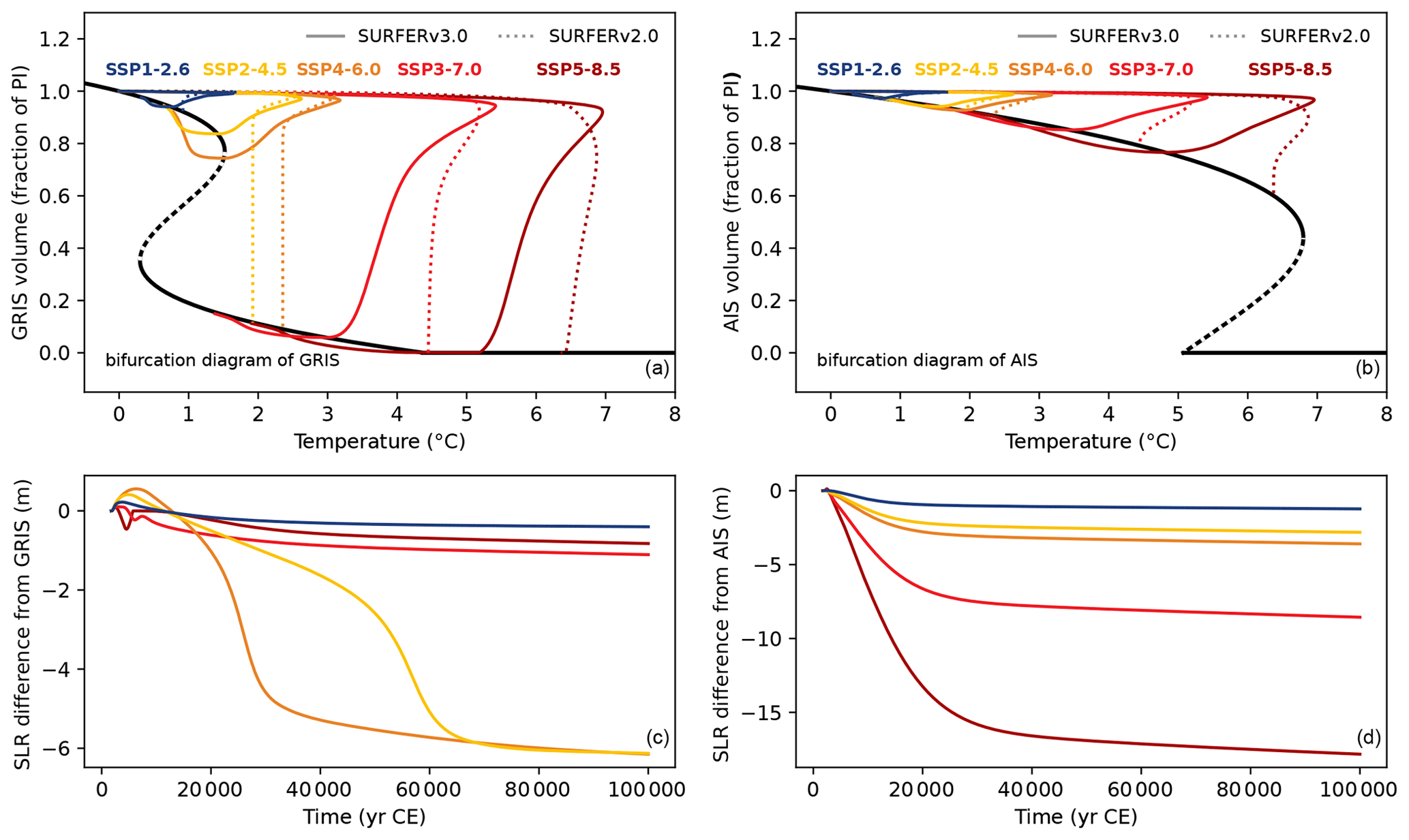
Figure 18 Comparison of Greenland and Antarctic sea level rise contributions in SURFER v3.0 and SURFER v2.0 for SSP emission scenarios. (a, b) Volume fractions of Greenland and Antarctica ice sheets as a function of temperature increase. Equilibrium values are shown in black, with stable equilibria represented by solid lines and unstable equilibria by dashed lines. (c, d) Difference in sea level rise contributions from Greenland and Antarctica in SURFER v3.0 and SURFER v2.0. Negatives values indicate a reduced sea level rise contribution in SURFER v3.0 compared to SURFER v2.0.

In SURFER, the ice sheets are designed as tipping elements (see Sect. 2.3). For both SURFER v2.0 and SURFER v3.0 and under all scenarios, the simulated temperature increase overshoots the critical warming threshold of the Greenland ice sheet. However, the Greenland ice sheet does not always collapse. Indeed, in general, tipping can be avoided if the overshoot duration is short relative to the effective timescale of the tipping element (Ritchie et al., 2019, 2021). For SURFER v2.0, this happens in the SSP1-2.6 scenario. For all other scenarios, the temperature stabilises past the critical threshold and thus Greenland eventually transitions to a completely melted state. In SURFER v3.0, thanks to a greater decrease in temperature after reaching a maximum, Greenland safely overshoots its critical threshold under the SSP2-4.5 and SSP4-6.0 scenarios as well. This happens even though peak warming reaches 2.62 and 3.18 °C, respectively, well above the Greenland ice sheet's critical threshold of 1.52 °C (as set in SURFER). For these scenarios, this leads to a ∼6 m reduction in the long-term sea level rise contribution simulated by SURFER v3.0 compared to SURFER v2.0.

Meanwhile, the Antarctic ice sheet does not tip in our simulations, regardless of whether SURFER v2.0 or SURFER v3.0 is used. This is because the critical warming threshold for the Antarctic ice sheet, set to 6.8 °C in SURFER, is much higher than that for Greenland and is seldom reached, even under the SSP5-8.5 scenario. However, despite no changes in the tipping behaviour, differences in simulated temperatures still give rise to large differences in the SLR contribution, particularly for high-emission scenarios. The long-term sea level rise contributions from Antarctica for the SSP3-7.0 and SSP5-8.5 scenarios are reduced by ∼8 and ∼18 m, respectively, in SURFER v3.0 compared to in SURFER v2.0.

5 Discussion

Our primary goal with SURFER v3.0 was to improve the representation of carbon cycle dynamics to enable simulations of the Earth system on multimillennial timescales. To this end, we have added to SURFER v2.0 a dynamic and more precise representation of alkalinity, an explicit representation of the carbonate and soft-tissue pumps, a sediment reservoir with associated accumulation and burial fluxes, and weathering, as well as volcanic out-gassing fluxes. We have shown that these additions allow for an accurate simulation of carbon cycle dynamics on multimillennial timescales by comparing SURFER v3.0 to the outputs from the LTMIP experiments and to the outputs of cGENIE for 1 Myr runs. Furthermore, we showed that the stabilisation of atmospheric CO₂ and temperature at lower levels in SURFER v3.0 than in SURFER v2.0 leads to a significant reduction in simulated sea level rise. While this outcome is robust, the tipping behaviour of the Greenland ice sheet in response to specific emission scenarios is sensitive to the choice of model parameters. For the parameter set used in this study (see Tables 2 and 3), we found that, in contrast to SURFER v2.0, Greenland avoids tipping in SURFER v3.0 under the intermediate-emission scenarios SSP2-4.5 and SSP4-6.0.

A secondary goal with SURFER v3.0 was to improve on SURFER v2.0 for the decadal to centennial timescales. This was done by adding an ocean layer of intermediate depth, temperature and pressure dependence of the solubility and dissociation constants, and a representation of atmospheric methane and by carefully setting the initial conditions of the oceanic variables based on the GLODAP dataset. We have shown that SURFER v3.0 successfully reproduces the historical CO₂ and CH₄ concentrations, the estimated historical land and ocean sinks, and the CMIP6 ensemble mean for the evolution of different quantities under the SSP1-2.6 and SSP3-7.0 scenarios and that in all these tasks, it performs equally well as or better than SURFER v2.0.

In summary, SURFER v3.0 outperforms SURFER v2.0 on all timescales, and despite having doubled the number of differential equations, it stays fast, transparent, and easy to modify. This paper contains all the equations for the model, all the parameter values, and the initial conditions for all the variables. SURFER v3.0 is coded in Python, which is one of the most widely used open-source programming languages. The code of the model, as well as the code for all the figures, is available online in a Jupyter notebook, providing a wide range of example use cases.

Of course, many coupled atmosphere–ocean box models of the carbon cycle already exist, some of them including carbonate sediments and weathering processes (Keir, 1988; Munhoven and François, 1996; Lenton and Britton, 2006; Zeebe, 2012; Köhler and Munhoven, 2020). These models, often primarily focused on the ocean, offer a more complex representation of the carbon cycle than SURFER v3.0. For instance, BICYCLE-SE (Köhler and Munhoven, 2020) includes 1 atmospheric box; 10 ocean boxes (5 surface boxes); ocean cycling of DIC, alkalinity, dissolved oxygen, and phosphate; sediment columns in each ocean basin and at various depths; and 7 terrestrial biosphere boxes. Still, despite being simpler, SURFER v3.0 effectively captures the essential dynamics of the carbon cycle, as demonstrated in the preceding sections.

Moreover, SURFER includes a dynamic representation of temperature and sea level rise, which is often lacking in other models, where those quantities are constant or prescribed. Among existing models, the one from Lenton and Britton (2006) is the closest to SURFER v3.0, with 4 ocean boxes, 10 sediment boxes, 2 terrestrial biosphere boxes, and a weathering flux parameterisation. As in SURFER v3.0, its carbon cycle is coupled with an energy balance representation of global mean temperature, and both models can be classified as “simple Earth system models”. While it is possible to integrate SURFER's temperature equations and sea level rise parameterisation into other models, we believe that the unique combination of processes included, simplicity, transparency, and speed makes SURFER v3.0 a valuable addition to the literature on top of being a worthwhile update to SURFER v2.0.

Although we are quite satisfied with SURFER's capabilities, we are certainly not claiming that it is the one model to rule them all. Indeed, its simplicity comes with several limitations that we discuss here.

First, SURFER v3.0 lacks horizontal resolution. In particular, SURFER v3.0 has no high-latitude ocean surface box, which is a feature of most ocean carbon cycle box models and could help to simulate the atmosphere-to-ocean CO₂ flux more realistically. The lack of spatial resolution also implies that SURFER v3.0 does not represent land temperatures, hence equating global mean temperatures with ocean mean surface temperatures. As shown in Sect. 4.1, this leads to an overestimation of ocean surface temperature and thermosteric SLR for historical and SSP forced runs.

Additionally, several oceanic and land carbon–climate feedbacks are missing in SURFER v3.0. For example, there is no dynamic ocean circulation, and as such, changes in atmosphere-to-ocean CO₂ fluxes resulting from climate-induced changes in the oceanic circulation are not represented. This was suggested in Sect. 3.3 by comparing the “climate feedback” of SURFER v3.0 with other models for the 5000 PgC pulse LTMIP experiment. A second example is the organic matter and CaCO₃ production in the upper-ocean layer that are kept constant, neglecting eventual changes in marine ecosystem production and associated carbon uptake. Last but not least is our parameterisation of atmosphere-to-land carbon flux, which depends on the atmospheric CO₂ concentration but not on temperature. As explained in Sect. 3.2, this is probably the reason why SURFER's land sink stays positive longer than other models under high-emission scenarios. Furthermore, this parameterisation does not account for hypothesised tipping elements such as the Amazon and boreal forests or the permafrost, which may release important amounts of greenhouse gases past critical warming thresholds (Armstrong McKay et al., 2022).

Moreover, SURFER lacks a detailed representation of land surface–vegetation–albedo feedbacks, which can influence temperatures and hydroclimate on decadal to multicentennial timescales through changes in vegetation cover (Forster et al., 2021; Willeit et al., 2014; Feng et al., 2022). In the current model, these feedbacks are indirectly represented via the climate feedback parameter β (see biogeophysical feedbacks in IPCC, 2021a, p. 976). However, they are not explicitly linked to the land carbon reservoir (M_L), the variable most closely associated with vegetation cover. This limitation, combined with the absence of a hydrological cycle and horizontal spatial resolution, constrains SURFER's ability to capture the full consequences of vegetation feedbacks. For example, SURFER may fail to account for their contribution to polar amplification (Willeit et al., 2014; Swann et al., 2010) and their subsequent impact on sea level changes. Simulations of the last glacial inception by Willeit et al. (2024) demonstrated that dynamic vegetation responses led to an additional 15 m decrease in sea level, highlighting the critical role of these feedbacks in shaping long-term Earth system trajectories.

For the sea level rise module, the contribution of the Antarctic ice sheet should probably be split into several components. Indeed, it has been shown that the West Antarctic ice sheet, as well as some East Antarctic subglacial basins, could collapse at lower warming thresholds than the East Antarctic ice sheet and could contribute several metres of sea level rise by 2300 under high-emission scenarios (Garbe et al., 2020; Alley et al., 2015; Coulon et al., 2024).

Finally, in its current state, SURFER v3.0 accounts for only one process influencing the carbon cycle on the 100 kyr timescale: the weathering of silicate rocks. Other potentially important processes acting on these timescales, such as orbital forcing variations, are currently neglected. These variations modulate the seasonal and spatial repartition of incoming solar energy and are known to drive or act as a pacemaker for the Quaternary glacial cycles (Hays et al., 1976).

Also neglected in SURFER, organic carbon burial may influence the climate system through its role in long-term carbon sequestration (Berner, 2004; Archer, 2010). For instance, during past oceanic anoxic events, reduced oxygen levels inhibited re-mineralisation processes, resulting in increased organic carbon preservation and burial in sediments and decreased atmospheric CO₂ levels (Schlanger and Jenkyns, 1976; Barclay et al., 2010). As warming is suspected to lead to oceanic deoxygenation due to reduced oxygen solubility and enhanced weathering fluxes (Schmittner et al., 2008; Ruvalcaba Baroni et al., 2020), organic carbon burial may act as a negative feedback mechanism that mitigates warming.

In addition, organic carbon plays a critical role in carbonate sedimentation. In oxic pore waters, the respiration of organic matter creates acidic micro-environments that enhance the dissolution of CaCO₃ sediments (Sarmiento and Gruber, 2006). Incorporating organic carbon burial into SURFER would require adding a sediment reservoir for organic carbon along with accumulation and burial fluxes, similar to the implementation of CaCO₃ burial. Ideally, the model should also account for the flux of organic carbon from land to the ocean through river input and exchange fluxes between ocean layers due to oceanic circulation. While these modifications are conceptually straightforward, parameterising the fluxes would require incorporating oxygen and nutrient cycling, which is essential to determine the rates of organic carbon production and re-mineralisation. Implementing these features would demand additional effort but offer a more comprehensive representation of the long-term carbon cycle and would enable the study of oceanic anoxic events.

6 Conclusions

We have presented SURFER v3.0, a simple Earth system model that includes a dynamic carbon cycle and simulates various important quantities such as atmospheric CO₂ and CH₄ concentrations, temperature anomalies, ocean surface pH, and sea level rise in response to anthropogenic greenhouse gas emissions. SURFER v3.0 extends SURFER v2.0 by incorporating dynamic alkalinity cycling, CaCO₃ sediments, and weathering processes. These additions enable SURFER v3.0 to accurately simulate the dynamics of the coupled carbon–climate system over timescales ranging from decades to millions of years. We have validated this by comparing SURFER v3.0 to historical data and outputs from global climate models (GCMs), EMICs, and other box models.

We have also demonstrated that SURFER v3.0 can simulate thermosteric sea level rise reasonably well on millennial timescales, although it tends to overestimate it on shorter timescales. Furthermore, we have shown that incorporating long-term carbon cycle processes in SURFER v3.0 leads to a significant reduction in the simulated contributions of Greenland and Antarctica to sea level rise compared to those in SURFER v2.0. These results highlight the critical importance of considering these processes to better predict committed sea level changes.

SURFER v3.0 is fast, transparent, and easy to modify and use, and hence it is an ideal tool for policy assessments that wish to take into account centennial to multimillennial timescales. In the future, we plan to add to SURFER a representation of glacial cycle dynamics and include several tipping elements to investigate the stability of the Earth system and the impact of anthropogenic emissions on its future long-term trajectories.

Appendix A: Emission scenarios

A1 Historical and SSP runs (Figs. 3–8, 16, 18, D1–D8)

For CO₂ emissions up to 1989 (inclusive), we use the data from the global carbon budget (Friedlingstein et al., 2022). Fossil emissions start in 1750, and we include the cement carbonation sink in them. Land use emissions are only provided from the year 1850, and so we assume that they have grown linearly from zero since 1750. This adds around 33 PgC of emissions compared to a scenario where land use emissions are considered zero before 1850.

For CH₄ emissions up to 1989 (inclusive), we use the data from Jones et al. (2023). Both fossil and land use emissions start in 1830, so, similarly to the CO₂ land use emissions, we assume that they increased linearly from 0 since 1750. This adds a total of ∼1147 Mt of CH₄ emissions compared to a scenario where land use and fossil CH₄ emissions are considered zero before 1830.

For all emissions (CO₂ and CH₄, fossil, and land use) from 1990 to 2100, we use the values provided in the SSP database (https://tntcat.iiasa.ac.at/SspDb/dsd, last access: 13 May 2025; Riahi et al., 2017; Gidden et al., 2019). All SSP scenarios have the same emissions between 1990 and 2015, so we perform our historical runs (1750–2014) with the values from any SSP scenario. The CO₂ and CH₄ emissions provided in 1990 by Friedlingstein et al. (2022) and Jones et al. (2023) are not equal to the values provided in 1990 in the SSP database, which causes small jumps in our emissions. For emissions between 2100 and 2300, we use the SSP extensions described in Meinshausen et al. (2020). Before the year 1750 and after the year 2300, all anthropogenic emissions are set to zero.

A2 Pulse experiments (Figs. 9–15)

For these experiments, the model is started with an additional amount of carbon x in the atmospheric reservoir, depending on the emission pulse: $M_{\mathrm{A}}\left(t_{\mathrm{PI}}\right)=\mathrm{580.3}+x$ PgC. No other emissions are used.

A3 Others (Fig. 17)

For the experiments in Sect. 4.1 where we compare SURFER to UVic, we use the CO₂ emissions provided in the supplementary material of Clark et al. (2016), while CH₄ emissions are set to zero.

Appendix B: Temperature and pressure dependance of solubility and dissociation constants

For the temperature (and salinity) dependence of K₀, K₁, K₂, K_b, K_w, and $K_{\mathrm{sp}}^{{\mathrm{CaCO}}_{\mathrm{3}}}$, we use the equations from Sarmiento and Gruber (2006), which are originally from Weiss (1974), Mehrbach et al. (1973), Dickson and Millero (1987), Millero (1995), Dickson (1990), and Mucci (1983):

$$\begin{array}{}\text{(B1)}& {\displaystyle }\begin{array}{rl}\ln K_{\mathrm{0}}& =-\mathrm{60.2409}+\mathrm{93.4517}\left({\displaystyle \frac{\mathrm{100}}{T}}\right)+\mathrm{23.3585}\\ & \cdot \ln \left({\displaystyle \frac{T}{\mathrm{100}}}\right)+S(\mathrm{0.023517}-\mathrm{0.023656}\left({\displaystyle \frac{T}{\mathrm{100}}}\right)\\ & +\mathrm{0.0047036}{\left({\displaystyle \frac{T}{\mathrm{100}}}\right)}^{\mathrm{2}})\end{array}\text{(B2)}& {\displaystyle }\begin{array}{rl}-\log K_{\mathrm{1}}^{\mathrm{0}}& =-\mathrm{62.008}+{\displaystyle \frac{\mathrm{3670.7}}{T}}+\mathrm{9.7944}\cdot \ln T\\ & -\mathrm{0.0118}\cdot S+\mathrm{0.000116}\cdot S^{\mathrm{2}},\end{array}\text{(B3)}& {\displaystyle }\begin{array}{rl}-\log K_{\mathrm{2}}^{\mathrm{0}}& =+\mathrm{4.777}+{\displaystyle \frac{\mathrm{1394.7}}{T}}-\mathrm{0.0184}\cdot S\\ & +\mathrm{0.000118}\cdot S^{\mathrm{2}},\end{array}\text{(B4)}& {\displaystyle }\begin{array}{rl}\ln K_{\mathrm{b}}^{\mathrm{0}}& ={\displaystyle \frac{\mathrm{1}}{T}}\left(-\mathrm{8966.9}-\mathrm{2890.53}\cdot S^{\mathrm{1}/\mathrm{2}}-\mathrm{77.942}\cdot S\right.\\ & \left.+\mathrm{1.728}\cdot S^{\mathrm{3}/\mathrm{2}}-\mathrm{0.0996}\cdot S^{\mathrm{2}}\right)+\mathrm{148.0248}\\ & +\mathrm{137.1942}\cdot S^{\mathrm{1}/\mathrm{2}}+\mathrm{1.62142}\cdot S+\mathrm{0.053105}\cdot S^{\mathrm{1}/\mathrm{2}}T\\ & +\ln T\left(-\mathrm{24.4344}-\mathrm{25.085}\cdot S^{\mathrm{1}/\mathrm{2}}-\mathrm{0.2474}\cdot S\right),\end{array}\text{(B5)}& {\displaystyle }\begin{array}{rl}\ln K_{\mathrm{w}}^{\mathrm{0}}& =\mathrm{148.96502}+{\displaystyle \frac{-\mathrm{13847.26}}{T}}-\mathrm{23.6521}\\ & \cdot \ln T{S}^{\mathrm{1}/\mathrm{2}}\left(-\mathrm{5.977}+{\displaystyle \frac{\mathrm{118.67}}{T}}+\mathrm{1.0495}\cdot \ln T\right)\\ & -\mathrm{0.01615}\cdot S,\end{array}\text{(B6)}& {\displaystyle }\begin{array}{rl}\ln K_{\mathrm{sp}}^{{\mathrm{CaCO}}_{\mathrm{3}},\mathrm{0}}& =-\mathrm{395.8293}+{\displaystyle \frac{\mathrm{6537.773}}{T}}+\mathrm{71.595}\cdot \ln T\\ & -\mathrm{0.17959}\cdot T+(-\mathrm{1.78938}+{\displaystyle \frac{\mathrm{410.64}}{T}}\\ & +\mathrm{0.0065453}\cdot T)S^{\mathrm{1}/\mathrm{2}}-\mathrm{0.17755}\cdot S\\ & +\mathrm{0.0094979}\cdot S^{\mathrm{2}/\mathrm{3}}.\end{array}\end{array}$$

Here, K₀, $K_{\mathrm{1}}^{\mathrm{0}}$, $K_{\mathrm{2}}^{\mathrm{0}}$, $K_{\mathrm{w}}^{\mathrm{0}}$, $K_{\mathrm{b}}^{\mathrm{0}}$, and $K_{\mathrm{sp}}^{{\mathrm{CaCO}}_{\mathrm{3}},\mathrm{0}}$ are the values of the constants at atmospheric pressure, given in mol (kg atm)⁻¹ for K₀; in mol kg⁻¹ for $K_{\mathrm{1}}^{\mathrm{0}}$, $K_{\mathrm{2}}^{\mathrm{0}}$, $K_{\mathrm{b}}^{\mathrm{0}}$; and in (mol kg⁻¹)² for $K_{\mathrm{w}}^{\mathrm{0}}$ and $K_{\mathrm{sp}}^{{\mathrm{CaCO}}_{\mathrm{3}},\mathrm{0}}$. T is the temperature in Kelvin, and S is the salinity on the practical salinity scale. In SURFER, only temperature anomalies are computed, meaning that to compute the absolute temperature and then the dissociation constants, we need to provide an initial temperature for each layer. This is done in Sect. 2.4.2.

The pressure (depth) dependence for K₁, K₂, K_w, K_b, and $K_{\mathrm{sp}}^{{\mathrm{CaCO}}_{\mathrm{3}}}$ is from Millero (1995),

$$\begin{array}{}\text{(B7)}& \ln \left(K_i^{\mathrm{p}}/K_i^{\mathrm{0}}\right)=-{\displaystyle \frac{\mathrm{\Delta }{V}_i}{RT}}P+{\displaystyle \frac{\mathrm{0.5}\mathrm{\Delta }{K}_i}{RT}}{P}^{\mathrm{2}},\end{array}$$

where $K_i^{\mathrm{p}}$ is the value of the dissociation constant at pressure P (in bar), $K_i^{\mathrm{0}}$ is the value of the dissociation constant at atmospheric pressure (1.01325 bar or 101 325 Pa), T is the temperature in Kelvin, and R is the gas constant in bar cm³ mol⁻¹ K⁻¹ (10 times the value in J mol⁻¹ K⁻¹). The quantities ΔV_i and ΔK_i are changes in molal volume and compressibility and are estimated following

$$\begin{array}{}\text{(B8)}& {\displaystyle }& {\displaystyle }\mathrm{\Delta }{V}_i=a_{\mathrm{0},i}+a_{\mathrm{1},i}(T-\mathrm{273.15})+a_{\mathrm{2},i}(T-\mathrm{273.15}{)}^{\mathrm{2}},\text{(B9)}& {\displaystyle }& {\displaystyle }\mathrm{1000}\mathrm{\Delta }{K}_i=b_{\mathrm{0},i}+b_{\mathrm{1},i}(T-\mathrm{273.15}).\end{array}$$

Values for the coefficients are in Table B1.

Table B1 Parameterisation for the effect of pressure on dissociation constants, the coefficients for Eqs. (B8) and (B9). The values are taken from Millero (1995). We have flipped the signs of a₁ and a₂ for K_b and b₁ for $K_{\mathrm{sp}}^{{\mathrm{CaCO}}_{\mathrm{3}}}$ to match the values given in Millero (1979).

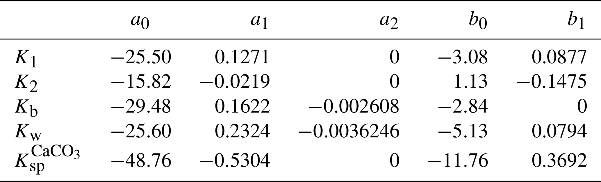
Hydrostatic balance provides the pressure at a given depth, thus, pressure (in bar) is given by $P=\mathit{\rho }gz/\mathrm{100}\mathrm{000}$, where ρ=1026 kg m⁻³ is the seawater mean density, g=9.81 kg m s⁻² is the gravitational acceleration, and z is the depth (in m). For the computation of mean quantities in the different ocean levels U, I, and D, we use the depths z_U=75 m, z_I=400 m, and z_D=2225 m, which correspond to the mid-depth points of the layers.

Appendix C: Alkalinity and solving the carbonate system

In SURFER v2.0, we approximated alkalinity using carbonate alkalinity,

$$\begin{array}{}\text{(C1)}& \mathrm{Alk}\approx {\mathrm{Alk}}_{\mathrm{C}}=\left[{\mathrm{HCO}}_{\mathrm{3}}^{-}\right]+\mathrm{2}\left[{\mathrm{CO}}_{\mathrm{3}}^{\mathrm{2}-}\right].\end{array}$$

To compute [H⁺] and the other carbonate species, we had to rewrite Eq. (C1) as a function of the four known quantities DIC, Alk, T, and S, and the unknown quantity [H⁺]. Using the definition of DIC (Eq. 11) and of the dissociation constants K₁ and K₂ (Eqs. 17 and 18), we can express DIC as a function of [${\mathrm{HCO}}_{\mathrm{3}}^{-}$] and [H⁺],

$$\begin{array}{}\text{(C2)}& \mathrm{DIC}=\left(\mathrm{1}+{\displaystyle \frac{K_{\mathrm{2}}}{\left[{\mathrm{H}}^{+}\right]}}+{\displaystyle \frac{\left[{\mathrm{H}}^{+}\right]}{K_{\mathrm{1}}}}\right)\left[{\mathrm{HCO}}_{\mathrm{3}}^{-}\right],\end{array}$$

or equivalently, we can express [${\mathrm{HCO}}_{\mathrm{3}}^{-}$] as a function of DIC and [H⁺],

$$\begin{array}{}\text{(C3)}& \left[{\mathrm{HCO}}_{\mathrm{3}}^{-}\right]={\displaystyle \frac{\mathrm{DIC}\cdot K_{\mathrm{1}}\left[{\mathrm{H}}^{+}\right]}{K_{\mathrm{1}}{K}_{\mathrm{2}}+K_{\mathrm{1}}\left[{\mathrm{H}}^{+}\right]+{\left[{\mathrm{H}}^{+}\right]}^{\mathrm{2}}}}.\end{array}$$

Using Eq. (18), we can then express [${\mathrm{CO}}_{\mathrm{3}}^{\mathrm{2}-}$] as a function of DIC and [H⁺]:

$$\begin{array}{}\text{(C4)}& \begin{array}{rl}\left[{\mathrm{CO}}_{\mathrm{3}}^{\mathrm{2}-}\right]& ={\displaystyle \frac{\left[{\mathrm{HCO}}_{\mathrm{3}}^{-}\right]K_{\mathrm{2}}}{\left[{\mathrm{H}}^{+}\right]}}\\ & ={\displaystyle \frac{\mathrm{DIC}\cdot K_{\mathrm{1}}{K}_{\mathrm{2}}}{K_{\mathrm{1}}{K}_{\mathrm{2}}+K_{\mathrm{1}}\left[{\mathrm{H}}^{+}\right]+{\left[{\mathrm{H}}^{+}\right]}^{\mathrm{2}}}}.\end{array}\end{array}$$

Inserting Eqs. (C3) and (C4) into Eq. (C1), we get

$$\begin{array}{}\text{(C5)}& {\mathrm{Alk}}_{\mathrm{C}}=\mathrm{DIC}\cdot {\displaystyle \frac{K_{\mathrm{1}}\left[{\mathrm{H}}^{+}\right]+K_{\mathrm{1}}{K}_{\mathrm{2}}}{K_{\mathrm{1}}{K}_{\mathrm{2}}+K_{\mathrm{1}}\left[{\mathrm{H}}^{+}\right]+{\left[{\mathrm{H}}^{+}\right]}^{\mathrm{2}}}},\end{array}$$

which we can solve for [H⁺], given Alk, DIC, and the dissociations constants K₁ and K₂ (which depend on T and S). To do so, we write Eq. (C5) as a second-degree polynomial equation:

$$\begin{array}{}\text{(C6)}& P_{\mathrm{C}}\left(\left[{\mathrm{H}}^{+}\right]\right)\equiv {\left[{\mathrm{H}}^{+}\right]}^{\mathrm{2}}+a_{\mathrm{1}}\left[{\mathrm{H}}^{+}\right]+a_{\mathrm{0}},\end{array}$$

with

$$\begin{array}{}\text{(C7)}& {\displaystyle }& {\displaystyle }{a}_{\mathrm{1}}=K_{\mathrm{1}}\left(\mathrm{1}-{\displaystyle \frac{\mathrm{DIC}}{\mathrm{Alk}}}\right),\text{(C8)}& {\displaystyle }& {\displaystyle }{a}_{\mathrm{0}}=K_{\mathrm{1}}{K}_{\mathrm{2}}\left(\mathrm{1}-{\displaystyle \frac{\mathrm{2}\cdot \mathrm{DIC}}{\mathrm{Alk}}}\right).\end{array}$$

The positive root is given by

$$\begin{array}{}\text{(C9)}& \begin{array}{rl}\left[{\mathrm{H}}^{+}\right]& ={\displaystyle \frac{K_{\mathrm{1}}}{\mathrm{2}\cdot \mathrm{Alk}}}\\ & (\sqrt{(\mathrm{DIC}-\mathrm{Alk}{)}^{\mathrm{2}}-\mathrm{4}{\displaystyle \frac{K_{\mathrm{2}}}{K_{\mathrm{1}}}}\mathrm{Alk}\cdot (\mathrm{Alk}-\mathrm{2}\cdot \mathrm{DIC})}\\ \\ & +(\mathrm{DIC}-\mathrm{Alk})).\end{array}\end{array}$$

Then, [${\mathrm{HCO}}_{\mathrm{3}}^{-}$] can be computed from Eq. (C3), [${\mathrm{CO}}_{\mathrm{3}}^{\mathrm{2}-}$] can be computed from Eq. (C4), and finally, [H₂CO₃^*] can be computed from Eq. (17).

In SURFER v3.0, we approximate alkalinity using the carbonate, borate, and water self-ionisation alkalinity:

$$\begin{array}{}\text{(C10)}& \begin{array}{rl}\mathrm{Alk}& \approx {\mathrm{Alk}}_{\mathrm{CBW}}=\left[{\mathrm{HCO}}_{\mathrm{3}}^{-}\right]+\mathrm{2}\left[{\mathrm{CO}}_{\mathrm{3}}^{\mathrm{2}-}\right]+\left[{\mathrm{OH}}^{-}\right]\\ & -\left[{\mathrm{H}}^{+}\right]+\left[\mathrm{B}(\mathrm{OH}{)}_{\mathrm{4}}^{-}\right].\end{array}\end{array}$$

As before, to compute [H⁺] and the other carbonate species, we have to rewrite Eq. (C10) as a function of the four known quantities, DIC, Alk, T, and S, and the unknown quantity [H⁺]. We already know how to express [${\mathrm{HCO}}_{\mathrm{3}}^{-}$] and [${\mathrm{CO}}_{\mathrm{3}}^{\mathrm{2}-}$] as a function of DIC and [H⁺] (Eqs. C3 and C4). Equation (19) further gives us

$$\begin{array}{}\text{(C11)}& \left[{\mathrm{OH}}^{-}\right]={\displaystyle \frac{K_{\mathrm{w}}}{\left[{\mathrm{H}}^{+}\right]}},\end{array}$$

and we can use Eqs. (20) and (21) to obtain

$$\begin{array}{}\text{(C12)}& \left[\mathrm{B}(\mathrm{OH}{)}_{\mathrm{4}}^{-}\right]={\displaystyle \frac{c_{\mathrm{b}}\cdot S\cdot K_{\mathrm{b}}}{\left[{\mathrm{H}}^{+}\right]+K_{\mathrm{b}}}}.\end{array}$$

Inserting these results in Eq. (C10), we get

$$\begin{array}{}\text{(C13)}& \begin{array}{rl}\mathrm{Alk}& \approx {\mathrm{Alk}}_{\mathrm{CBW}}=\mathrm{DIC}\cdot {\displaystyle \frac{K_{\mathrm{1}}\left[{\mathrm{H}}^{+}\right]+K_{\mathrm{1}}{K}_{\mathrm{2}}}{K_{\mathrm{1}}{K}_{\mathrm{2}}+K_{\mathrm{1}}\left[{\mathrm{H}}^{+}\right]+{\left[{\mathrm{H}}^{+}\right]}^{\mathrm{2}}}}\\ & +{\displaystyle \frac{K_{\mathrm{w}}}{\left[{\mathrm{H}}^{+}\right]}}-\left[{\mathrm{H}}^{+}\right]+{\displaystyle \frac{c_{\mathrm{b}}\cdot S\cdot K_{\mathrm{b}}}{\left[{\mathrm{H}}^{+}\right]+K_{\mathrm{b}}}},\end{array}\end{array}$$

which we can use to solve for [H⁺] given Alk; DIC; and the dissociation constants K₁, K₂, K_w, and K_b (which depend on T and S). To do this, we follow Munhoven (2013), and we write Eq. (C13) as a polynomial equation that is now fifth degree:

$$\begin{array}{}\text{(C14)}& \begin{array}{rl}{P}_{\mathrm{CBW}}\left(\left[{\mathrm{H}}^{+}\right]\right)& \equiv {\left[{\mathrm{H}}^{+}\right]}^{\mathrm{5}}+q_{\mathrm{4}}{\left[{\mathrm{H}}^{+}\right]}^{\mathrm{4}}+q_{\mathrm{3}}{\left[{\mathrm{H}}^{+}\right]}^{\mathrm{3}}\\ & +q_{\mathrm{2}}{\left[{\mathrm{H}}^{+}\right]}^{\mathrm{2}}+q_{\mathrm{1}}\left[{\mathrm{H}}^{+}\right]+q_{\mathrm{0}},\end{array}\end{array}$$

with

$$\begin{array}{}\text{(C15)}& {\displaystyle }{q}_{\mathrm{4}}=\mathrm{Alk}+K_{\mathrm{1}}+K_{\mathrm{b}},\text{(C16)}& {\displaystyle }\begin{array}{rl}{q}_{\mathrm{3}}& =\left(\mathrm{Alk}-\mathrm{DIC}+K_{\mathrm{b}}\right)K_{\mathrm{1}}+\left(\mathrm{Alk}-c_{\mathrm{b}}\cdot S\right)K_{\mathrm{b}}\\ & +K_{\mathrm{1}}{K}_{\mathrm{2}}-K_{\mathrm{w}},\end{array}\text{(C17)}& {\displaystyle }\begin{array}{rl}{q}_{\mathrm{2}}& =\left(\mathrm{Alk}-\mathrm{2}\cdot \mathrm{DIC}+K_{\mathrm{b}}\right)K_{\mathrm{1}}{K}_{\mathrm{2}}+\left(\mathrm{Alk}-\mathrm{DIC}\right.\\ & \left.-c_{\mathrm{b}}\cdot S\right)K_{\mathrm{1}}{K}_{\mathrm{b}}-K_{\mathrm{1}}{K}_{\mathrm{w}}-K_{\mathrm{b}}{K}_{\mathrm{w}},\end{array}\text{(C18)}& {\displaystyle }\begin{array}{rl}{q}_{\mathrm{1}}& =\left(\mathrm{Alk}-\mathrm{2}\cdot \mathrm{DIC}-c_{\mathrm{b}}\cdot S\right)K_{\mathrm{1}}{K}_{\mathrm{2}}{K}_{\mathrm{b}}-K_{\mathrm{1}}{K}_{\mathrm{2}}{K}_{\mathrm{w}}\\ & -K_{\mathrm{1}}{K}_{\mathrm{b}}{K}_{\mathrm{w}},\end{array}\text{(C19)}& {\displaystyle }{q}_{\mathrm{0}}=-K_{\mathrm{1}}{K}_{\mathrm{2}}{K}_{\mathrm{b}}{K}_{\mathrm{w}}.\end{array}$$

We solve this equation using the Newton–Raphson method. To ensure quick convergence, we need a good initial guess that is not too far from the real solution. We adopt the following procedure from Munhoven (2013) and Humphreys et al. (2022). We define the following coefficients:

$$\begin{array}{}\text{(C20)}& {\displaystyle }& {\displaystyle }{c}_{\mathrm{2}}=K_{\mathrm{b}}\left(\mathrm{1}-{\displaystyle \frac{c_{\mathrm{b}}\cdot S}{\mathrm{Alk}}}\right)+K_{\mathrm{1}}\left(\mathrm{1}-{\displaystyle \frac{\mathrm{DIC}}{\mathrm{Alk}}}\right),\text{(C21)}& {\displaystyle }& {\displaystyle }{c}_{\mathrm{1}}=K_{\mathrm{1}}{K}_{\mathrm{b}}\left(\mathrm{1}-{\displaystyle \frac{c_{\mathrm{b}}\cdot S}{\mathrm{Alk}}}-{\displaystyle \frac{\mathrm{DIC}}{\mathrm{Alk}}}\right)+K_{\mathrm{1}}{K}_{\mathrm{2}}\left(\mathrm{1}-\mathrm{2}{\displaystyle \frac{\mathrm{DIC}}{\mathrm{Alk}}}\right),\text{(C22)}& {\displaystyle }& {\displaystyle }{c}_{\mathrm{0}}=K_{\mathrm{1}}{K}_{\mathrm{2}}{K}_{\mathrm{b}}\left(\mathrm{1}-{\displaystyle \frac{\mathrm{2}\cdot \mathrm{DIC}+c_{\mathrm{b}}\cdot S}{\mathrm{Alk}}}\right),\end{array}$$

from which we construct the quantities

$$\begin{array}{}\text{(C23)}& H_{\min }={\displaystyle \frac{-c_{\mathrm{2}}+\sqrt{c_{\mathrm{2}}^{\mathrm{2}}-\mathrm{3}{c}_{\mathrm{1}}}}{\mathrm{3}}},\end{array}$$

and

$$\begin{array}{}\text{(C24)}& H_{\mathrm{0}}=H_{\min }+\sqrt{-{\displaystyle \frac{H_{\min }^{\mathrm{3}}+c_{\mathrm{2}}{H}_{\min }^{\mathrm{2}}+c_{\mathrm{1}}{H}_{\min }+c_{\mathrm{0}}}{\sqrt{c_{\mathrm{2}}^{\mathrm{2}}-\mathrm{3}{c}_{\mathrm{1}}}}}}.\end{array}$$

The initial guess for the Newton–Raphson method is taken as

$$\begin{array}{}\text{(C25)}& \begin{array}{rl}& {\left[{\mathrm{H}}^{+}\right]}_{\mathrm{0}}=\\ & \left\{\begin{array}{ll}{\mathrm{10}}^{-\mathrm{3}}& \mathrm{if}\mathrm{Alk}\le \mathrm{0},\\ H_{\mathrm{0}}& \mathrm{if}\mathrm{0}<\mathrm{Alk}<\mathrm{2}\cdot \mathrm{DIC}+c_{\mathrm{b}}\cdot S\mathrm{and}{c}_{\mathrm{2}}^{\mathrm{2}}-\mathrm{3}{c}_{\mathrm{1}}>\mathrm{0},\\ {\mathrm{10}}^{-\mathrm{7}}& \mathrm{if}\mathrm{0}<\mathrm{Alk}<\mathrm{2}\cdot \mathrm{DIC}+c_{\mathrm{b}}\cdot S\mathrm{and}{c}_{\mathrm{2}}^{\mathrm{2}}-\mathrm{3}{c}_{\mathrm{1}}<\mathrm{0},\\ {\mathrm{10}}^{-\mathrm{10}}& \mathrm{if}\mathrm{Alk}\ge \mathrm{2}\cdot \mathrm{DIC}+c_{\mathrm{b}}\cdot S.\end{array}\right.\end{array}\end{array}$$

The rationale behind this choice is given in Munhoven (2013) and Humphreys et al. (2022). With it, we only need five Newton–Raphson iterations to obtain an accurate value for [H⁺] and pH, which is defined as

$$\begin{array}{}\text{(C26)}& \mathrm{pH}=-{\log }_{\mathrm{10}}\left(\left[{\mathrm{H}}^{+}\right]\right).\end{array}$$

Once [H⁺] is computed, [${\mathrm{HCO}}_{\mathrm{3}}^{-}$] and [${\mathrm{CO}}_{\mathrm{3}}^{\mathrm{2}-}$] can be computed from Eqs. (C3) and (C4), [${\mathrm{H}}_{\mathrm{2}}{\mathrm{CO}}_{\mathrm{3}}^{*}$] can be computed from Eq. (17), [OH⁻] can be computed from Eq. (C11), and [B(OH)${}_{\mathrm{4}}^{-}$] can be computed from Eq. (C12). Equation (C10) is solved following this procedure at every time step of the numerical integration of the model. This is because we need [H⁺]_U for the computation of B_U in the atmosphere to upper-ocean carbon flux F_A→U (see Eqs. 27 and 28), and we need [${\mathrm{CO}}_{\mathrm{3}}^{\mathrm{2}-}$]_D for the computation of the dissolution flux F_diss (see Eq. 48). This is also the procedure used to obtain climatologies (and vertical profiles) of the carbonate species from the GLODAP climatologies of DIC, Alk, temperature, and salinity (see Fig. 3). In this case, we computed the carbonate species at each ocean point where DIC, Alk, temperature, and salinity were all given.

To determine the initial conditions for the dissolved inorganic carbon mass in the upper layer M_U(t_PI), we need to compute DIC_U(t_PI) as a function of Alk_U(t_PI), T_U(t_PI), S_U, and[${\mathrm{H}}_{\mathrm{2}}{\mathrm{CO}}_{\mathrm{3}}^{*}$]_U(t_PI), which is fixed by equilibrium conditions (Eq. 108). Now DIC is an unknown, and we cannot use the procedure described above. Instead, we write Alk as a function of [${\mathrm{H}}_{\mathrm{2}}{\mathrm{CO}}_{\mathrm{3}}^{*}$] and [H⁺] (and the dissociation constants). Using Eqs. (17) and (18), we get

$$\begin{array}{}\text{(C27)}& {\displaystyle }& {\displaystyle }\left[{\mathrm{HCO}}_{\mathrm{3}}^{-}\right]={\displaystyle \frac{K_{\mathrm{1}}\left[{\mathrm{H}}_{\mathrm{2}}{\mathrm{CO}}_{\mathrm{3}}^{*}\right]}{\left[{\mathrm{H}}^{+}\right]}},\text{(C28)}& {\displaystyle }& {\displaystyle }\left[{\mathrm{CO}}_{\mathrm{3}}^{\mathrm{2}-}\right]={\displaystyle \frac{K_{\mathrm{1}}{K}_{\mathrm{2}}\left[{\mathrm{H}}_{\mathrm{2}}{\mathrm{CO}}_{\mathrm{3}}^{*}\right]}{{\left[{\mathrm{H}}^{+}\right]}^{\mathrm{2}}}},\end{array}$$

and thus

$$\begin{array}{}\text{(C29)}& \begin{array}{rl}\mathrm{Alk}& \approx {\mathrm{Alk}}_{\mathrm{CBW}}={\displaystyle \frac{K_{\mathrm{1}}\left[{\mathrm{H}}_{\mathrm{2}}{\mathrm{CO}}_{\mathrm{3}}^{*}\right]}{\left[{\mathrm{H}}^{+}\right]}}+\mathrm{2}{\displaystyle \frac{K_{\mathrm{1}}{K}_{\mathrm{2}}\left[{\mathrm{H}}_{\mathrm{2}}{\mathrm{CO}}_{\mathrm{3}}^{*}\right]}{{\left[{\mathrm{H}}^{+}\right]}^{\mathrm{2}}}}\\ & +{\displaystyle \frac{K_{\mathrm{w}}}{\left[{\mathrm{H}}^{+}\right]}}-\left[{\mathrm{H}}^{+}\right]+{\displaystyle \frac{c_{\mathrm{b}}\cdot S\cdot K_{\mathrm{b}}}{\left[{\mathrm{H}}^{+}\right]+K_{\mathrm{b}}}}.\end{array}\end{array}$$

This equation can be solved numerically for [H⁺] using any algorithm. The speed of the algorithm is not of great importance here since we only perform the computation for the setting of the initial conditions and not at each time step of the numerical integration. Once [H⁺] is obtained, [${\mathrm{HCO}}_{\mathrm{3}}^{-}$] and [${\mathrm{CO}}_{\mathrm{3}}^{\mathrm{2}-}$] are recovered with Eqs. (17) and (18), and DIC can then be computed as the sum of [${\mathrm{HCO}}_{\mathrm{3}}^{-}$], [${\mathrm{CO}}_{\mathrm{3}}^{\mathrm{2}-}$], and [${\mathrm{H}}_{\mathrm{2}}{\mathrm{CO}}_{\mathrm{3}}^{*}$].

Appendix D: Sensitivity analysis

We present here a sensitivity analysis of the model in response to changes in specific parameters. While the primary goal is to assess how these sometimes arbitrary parameter choices affect model behaviour, an added benefit is the ability to investigate the timescales on which the associated processes are significant.

We first test how atmospheric CO₂ levels simulated for the SSP3-7.0 scenario from 1750 to 1 000 000 CE respond to changes in 20 parameters associated with the carbon cycle component of SURFER v3.0 (all parameters from the first part of Table 2 except ${\mathit{\tau }}_{{\mathrm{CH}}_{\mathrm{4}}}$). Most parameters are adjusted one at a time, with interdependent parameters and M_U(t_PI) being modified accordingly to obey the preindustrial equilibrium condition (see second part of Table 2). Each parameter is varied within a range of 0.25 to 1.75 times its default value. Note that these ranges do not necessarily reflect physically plausible values.

Changing k_A→U in the range described above has a negligible impact on the atmospheric CO₂ draw-down (Fig. D1). This is because regardless of the values set for k_A→U, the transfer rate of CO₂ between the atmosphere and the ocean surface layer is very fast compared to the subsequent transport of dissolved carbon at depth, which is therefore the real limiting factor for oceanic CO₂ uptake. Indeed, we observe that increasing k_U→I or k_I→D leads to increased CO₂ uptake for up to 100 kyr. After that, the ocean, atmosphere, and sediment reservoirs are in equilibrium, and atmospheric CO₂ is regulated by the imbalance between volcanism and weathering. Changing k_I→D only has a very small effect before 2100 CE, reflecting the longer timescales associated with the deeper ocean. Note that we have varied ${\stackrel{\mathrm{̃}}{k}}_{\mathrm{U}\to \mathrm{I}}$ and ${\stackrel{\mathrm{̃}}{k}}_{\mathrm{I}\to \mathrm{D}}$ simultaneously as k_U→I and k_I→D because these parameters are all linked to the implicit ocean circulation.

Figure D2 shows the sensitivity of atmospheric CO₂ to changes in parameters associated with the carbonate and soft-tissue pumps. Overall, varying these parameters has a small or negligible impact. This is due to the preindustrial equilibrium condition that we impose, which creates a compensating effect. For example, if we have stronger pumps initially, we need stronger upwelling fluxes at equilibrium and so higher k_I→U and k_D→I (and ${\stackrel{\mathrm{̃}}{k}}_{\mathrm{I}\to \mathrm{U}}$ and ${\stackrel{\mathrm{̃}}{k}}_{\mathrm{D}\to \mathrm{I}}$). This leads to weaker $F_{\mathrm{U}\to \mathrm{I}}^{\mathrm{res}}$ and $F_{\mathrm{I}\to \mathrm{D}}^{\mathrm{res}}$ (and ${\stackrel{\mathrm{̃}}{F}}_{\mathrm{U}\to \mathrm{I}}^{\mathrm{res}}$ and ${\stackrel{\mathrm{̃}}{F}}_{\mathrm{U}\to \mathrm{I}}^{\mathrm{res}}$) fluxes, which mostly compensates for the effects of stronger pumps in transient runs (see Eqs. 43–46). This compensation effect is not exact, and we can observe a small impact of changes in P^org and ${\mathit{\varphi }}_{\mathrm{I}}^{\mathrm{org}}$. In comparison, the impacts of changes in $P^{{\mathrm{CaCO}}_{\mathrm{3}}}$, ${\mathit{\varphi }}_{\mathrm{I}}^{{\mathrm{CaCO}}_{\mathrm{3}}}$, and σ_Alk:DIC are almost nonexistent because these parameters are associated with smaller DIC and alkalinity fluxes. Changing ${\mathit{\varphi }}_{\mathrm{D}}^{{\mathrm{CaCO}}_{\mathrm{3}}}$ has no impact on model results because we keep $P^{{\mathrm{CaCO}}_{\mathrm{3}}}$ constant. In this case, the terms in F_acc involving ${\mathit{\varphi }}_{\mathrm{D}}^{{\mathrm{CaCO}}_{\mathrm{3}}}$ cancel out (see Eqs. 35, 48, and 101). Still, we have kept the parameter to facilitate further model updates. Increasing P^org implies that we need stronger upwelling fluxes to respect the preindustrial condition, and so overall the ocean is better ventilated, and it is harder to store carbon in the deep ocean, slowing down atmospheric CO₂ uptake. Increasing ${\mathit{\varphi }}_{\mathrm{I}}^{\mathrm{org}}$ has the opposite effect: it leads to a weaker soft-tissue pump, which implies weaker upwelling fluxes and thus faster CO₂ uptake.

Figures D3 and D4 show the sensitivity of atmospheric CO₂ to changes in parameters associated with the dissolution of CaCO₃ sediments and with weathering fluxes. Atmospheric CO₂ is sensitive to changes in α_diss and γ_diss but barely sensitive to changes in β_diss, meaning that the deep-${\mathrm{CO}}_{\mathrm{3}}^{\mathrm{2}-}$ concentration rather than the mass of erodible CaCO₃ sediments, M_S, is the dominant driver of dissolution in our parameterisation. With the biggest changes in atmospheric CO₂ concentration observed between 3000 CE and 50 kyr, these experiments showcase the timescales associated with sediment processes nicely. Changes in $F_{{\mathrm{CaCO}}_{\mathrm{3}},\mathrm{0}}$ and k_Ca associated with carbonate weathering have an negligible impact on CO₂ levels compared to changes in $F_{{\mathrm{CaSiO}}_{\mathrm{3}},\mathrm{0}}$ and k_T, which are associated with silicate weathering. This results from silicate weathering rather than carbonate weathering being the process that is ultimately responsible for the draw-down of excess atmospheric CO₂, at least in our model. We observe that a larger initial silicate weathering flux ($F_{{\mathrm{CaSiO}}_{\mathrm{3}},\mathrm{0}}$) or a larger response of silicate weathering to warming (k_T) leads to a faster uptake of CO₂, mostly noticeable after 100 kyr.

Focusing on vegetation in Fig. D5, we observe that the impact of varying k_A→L is small and limited to years before 2300 CE. This is because the exchanges of carbon between the atmosphere and the land are relatively fast, and so the limiting factor for land uptake is instead the amount of carbon that land can store, which is controlled by β_L. A larger β_L means that more carbon can be stored in the land reservoir for a given atmospheric concentration, thus increasing the land sink. Together with k_U→I and k_I→D (and ${\stackrel{\mathrm{̃}}{k}}_{\mathrm{U}\to \mathrm{I}}$ and ${\stackrel{\mathrm{̃}}{k}}_{\mathrm{I}\to \mathrm{D}}$), β_L is the parameter that has the biggest influence on CO₂ uptake up to the year ∼6500 CE, showing that the fertilisation effect and oceanic invasion of CO₂ are the main processes driving atmospheric CO₂ draw-down on these timescales in SURFER v3.0.

We also test how simulated atmospheric CO₂ levels, temperatures, and sea level rise respond to changes in γ_U→I, γ_I→D, and β, which are the parameters linked to the climate module of SURFER v3.0. The experimental setup is the same as the one described above.

Figures D6 and D7 show the sensitivity analysis for γ_U→I and γ_I→D. Increasing γ_U→I decreases the heat accumulation and thus temperatures in the surface layer but increases temperature in the intermediate and deep layers. On the other hand, increasing γ_I→D decreases the heat accumulation and temperature in the surface and intermediate layers but increases the temperature in the deep layer. For both parameters, an increase leads to an overall increase in thermosteric sea level rise because the deep layer dominates the thermal expansion. Although both parameters impact surface temperature, they have almost no impact on atmospheric CO₂ because SURFER v3.0 has a very weak carbon–climate feedback (see discussion, Sect. 5). We also observe little to no impact on temperatures after 10 000 kyr, suggesting that by that time, the ocean has reached thermal equilibrium.

In Fig. D8, we investigate the SURFER v3.0 response to changes in β, the climate feedback parameter. Decreasing β while keeping F_2× constant increases the equilibrium climate sensitivity. In this case, we vary β in the range of 0.780–1.671 W m⁻² °C⁻¹, giving an equilibrium climate sensitivity (ECS) range of 2.33–5 °C, which is within the estimated very likely 2–5 °C range given by the IPCC (Forster et al., 2021). Lower values for β, and thus higher values of climate sensitivity, naturally lead to more warming and consequently a higher sea level rise. Big differences in projected sea level rise after 10 kyr, even for close β values, are the consequence of the tipping of the Greenland ice sheet. As for γ_U→I and γ_I→D, changes in β do not impact CO₂ levels that much since the total carbon–climate feedback in SURFER v3.0 is weak. For higher values of climate sensitivity, the positive climate–carbon feedback resulting from the temperature-dependent solubility and dissociation constants leads to higher CO₂ levels up to around 10 kyr. Conversely, the negative carbon–climate feedback from silicate weathering, acting on longer timescales, results in lower CO₂ values after 10 kyr and especially after 100 000 kyr.

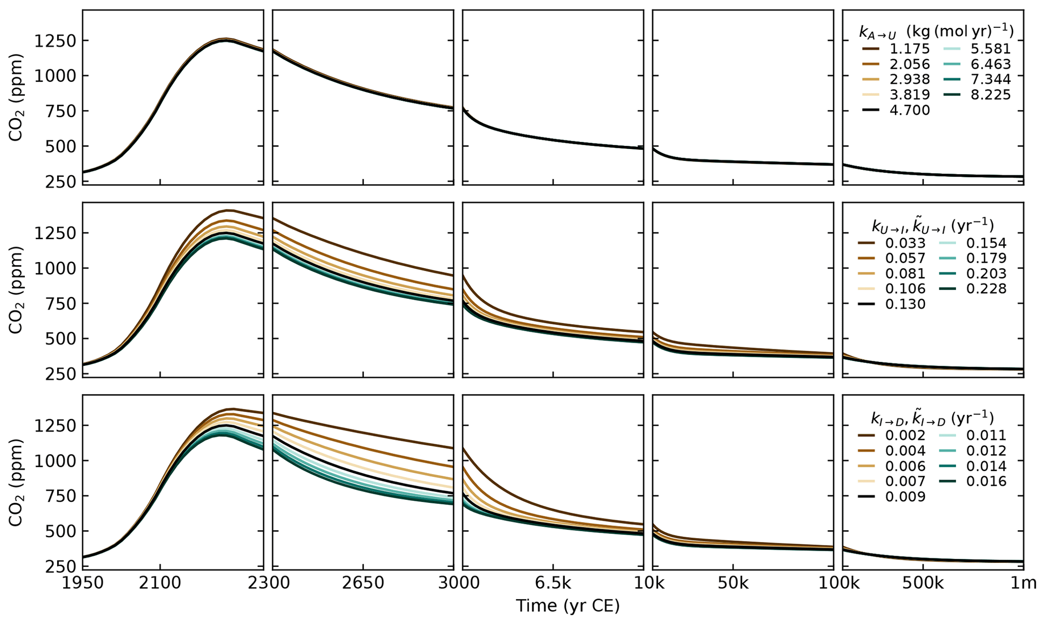
Figure D1 Atmospheric CO₂ concentration simulated by SURFER v3.0 under the SSP3-7.0 scenario for different values of k_A→U, k_U→I, and k_I→D (and ${\stackrel{\mathrm{̃}}{k}}_{\mathrm{U}\to \mathrm{I}}$ and ${\stackrel{\mathrm{̃}}{k}}_{\mathrm{I}\to \mathrm{D}}$). Black lines indicate the atmospheric CO₂ concentration simulated for the default parameter values, as described in Sect. 2.4.1.

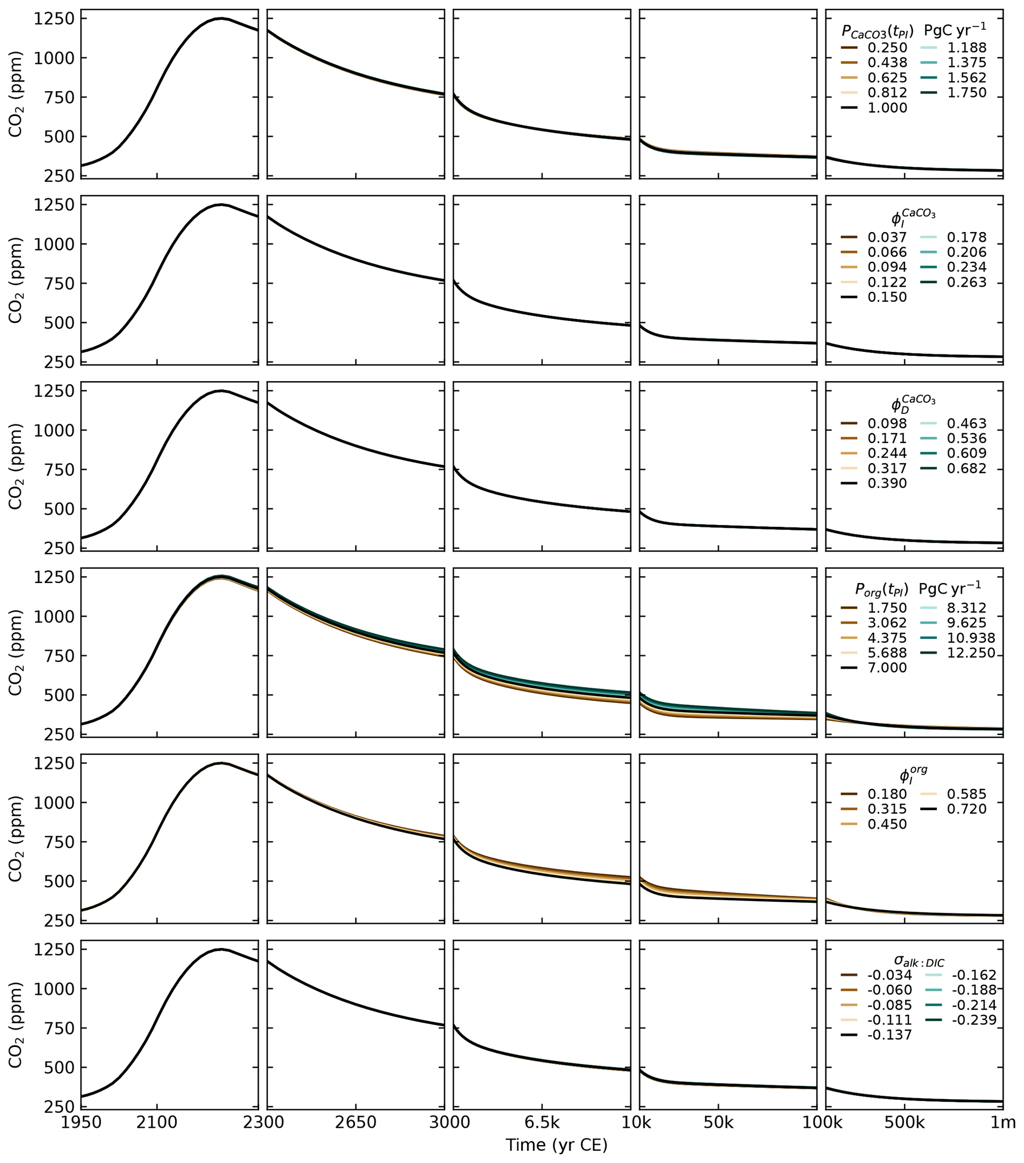
Figure D2 Atmospheric CO₂ concentration simulated by SURFER v3.0 under the SSP3-7.0 scenario for different values of $P^{{\mathrm{CaCO}}_{\mathrm{3}}}$, ${\mathit{\varphi }}_{\mathrm{I}}^{{\mathrm{CaCO}}_{\mathrm{3}}}$, ${\mathit{\varphi }}_{\mathrm{D}}^{{\mathrm{CaCO}}_{\mathrm{3}}}$, P^org, ${\mathit{\varphi }}_{\mathrm{I}}^{\mathrm{org}}$, and σ_Alk:DIC. Black lines indicate the atmospheric CO₂ concentration simulated for the default parameter values, as described in Sect. 2.4.1.

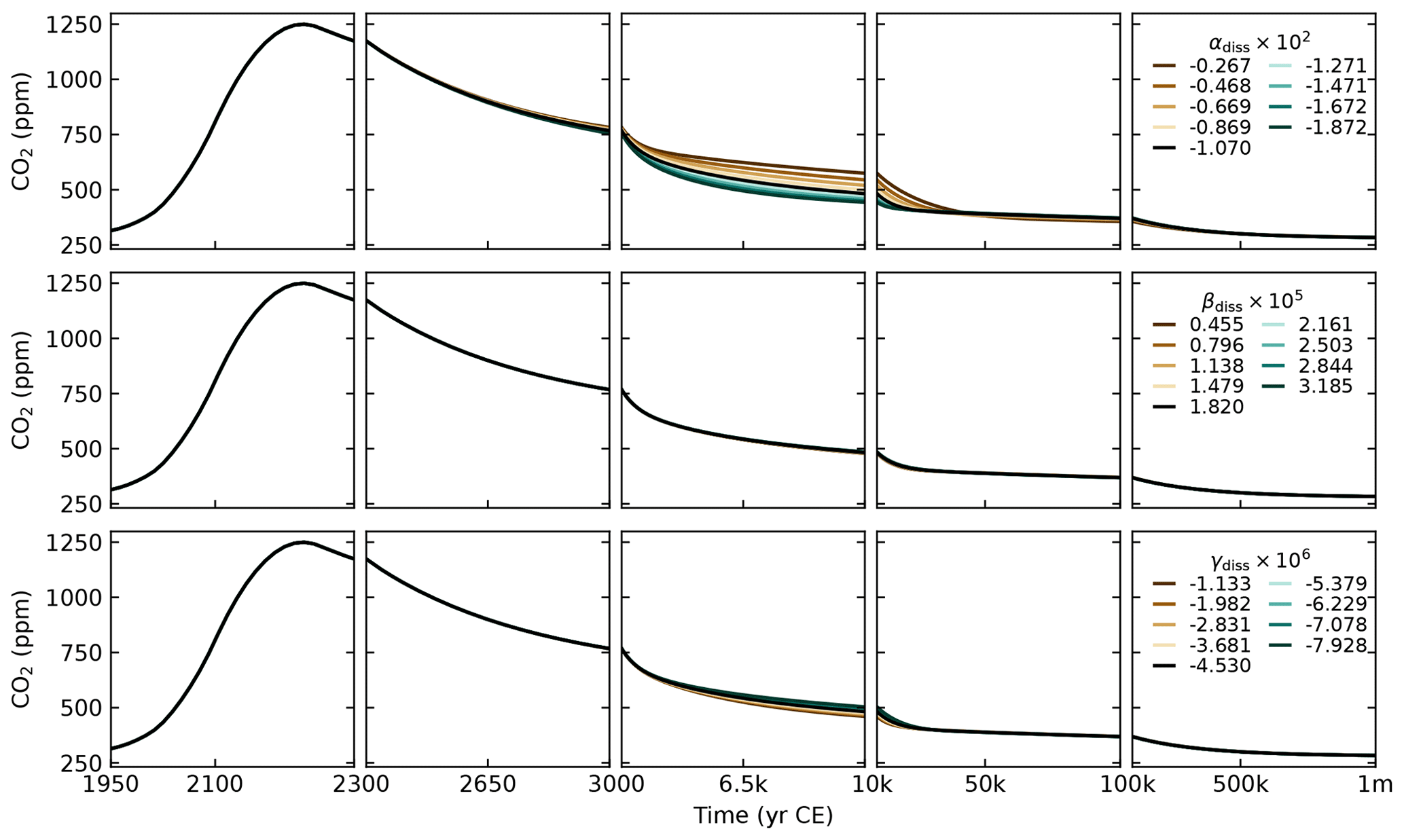
Figure D3 Atmospheric CO₂ concentration simulated by SURFER v3.0 under the SSP3-7.0 scenario for different values of α_diss, β_diss, and γ_diss. Black lines indicate the atmospheric CO₂ concentration simulated for the default parameter values, as described in Sect. 2.4.1.

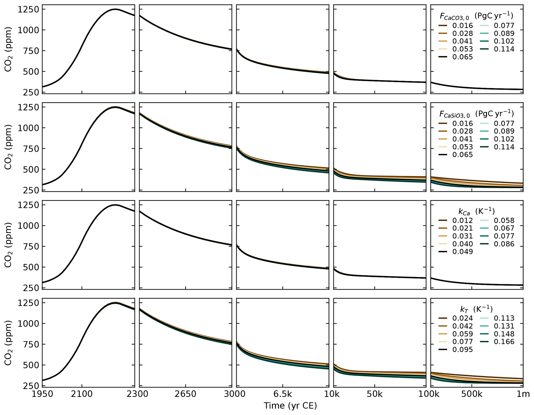
Figure D4 Atmospheric CO₂ concentration simulated by SURFER v3.0 under the SSP3-7.0 scenario for different values of $F_{{\mathrm{CaCO}}_{\mathrm{3}},\mathrm{0}}$, $F_{{\mathrm{CaSiO}}_{\mathrm{3}},\mathrm{0}}$, k_Ca, and k_T. Black lines indicate the atmospheric CO₂ concentration simulated for the default parameter values, as described in Sect. 2.4.1.

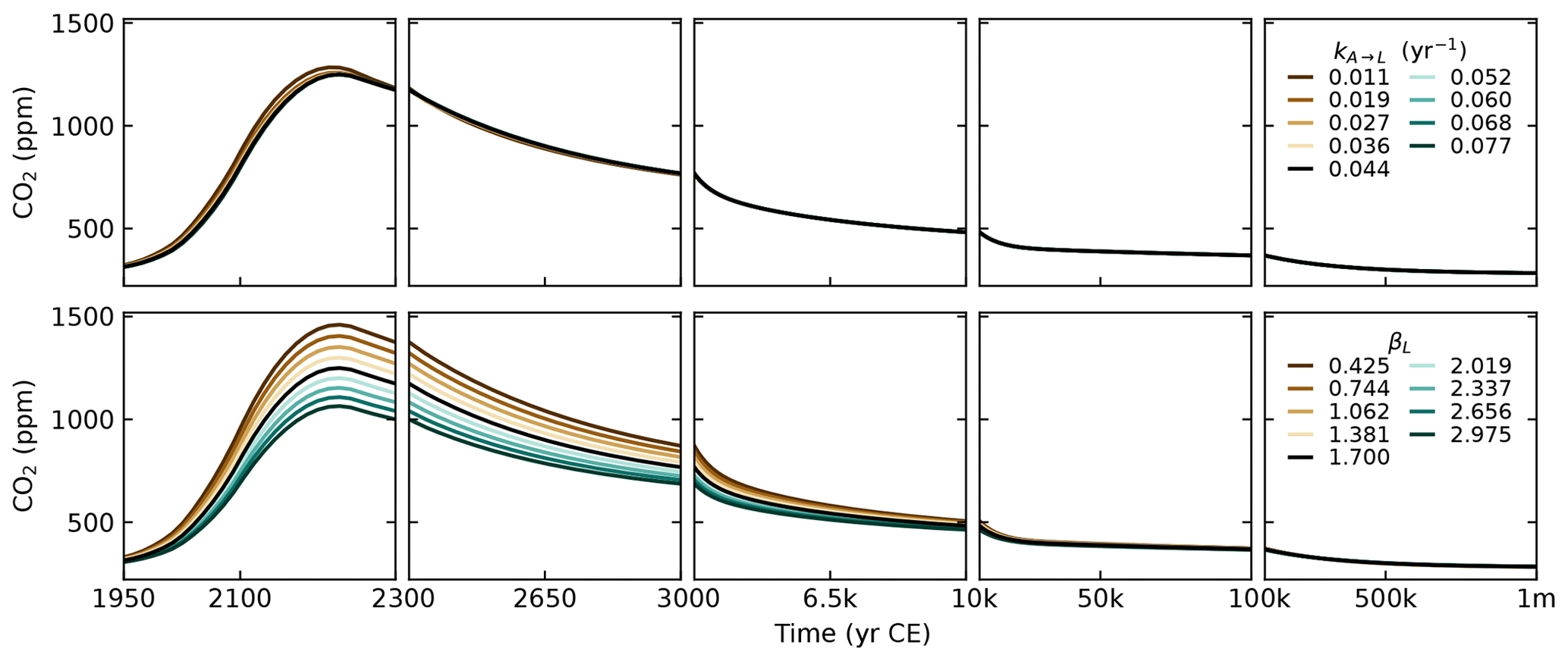
Figure D5 Atmospheric CO₂ concentration simulated by SURFER v3.0 under the SSP3-7.0 scenario for different values of k_A→L and β_L. Black lines indicate the atmospheric CO₂ concentration simulated for the default parameter values, as described in Sect. 2.4.1.

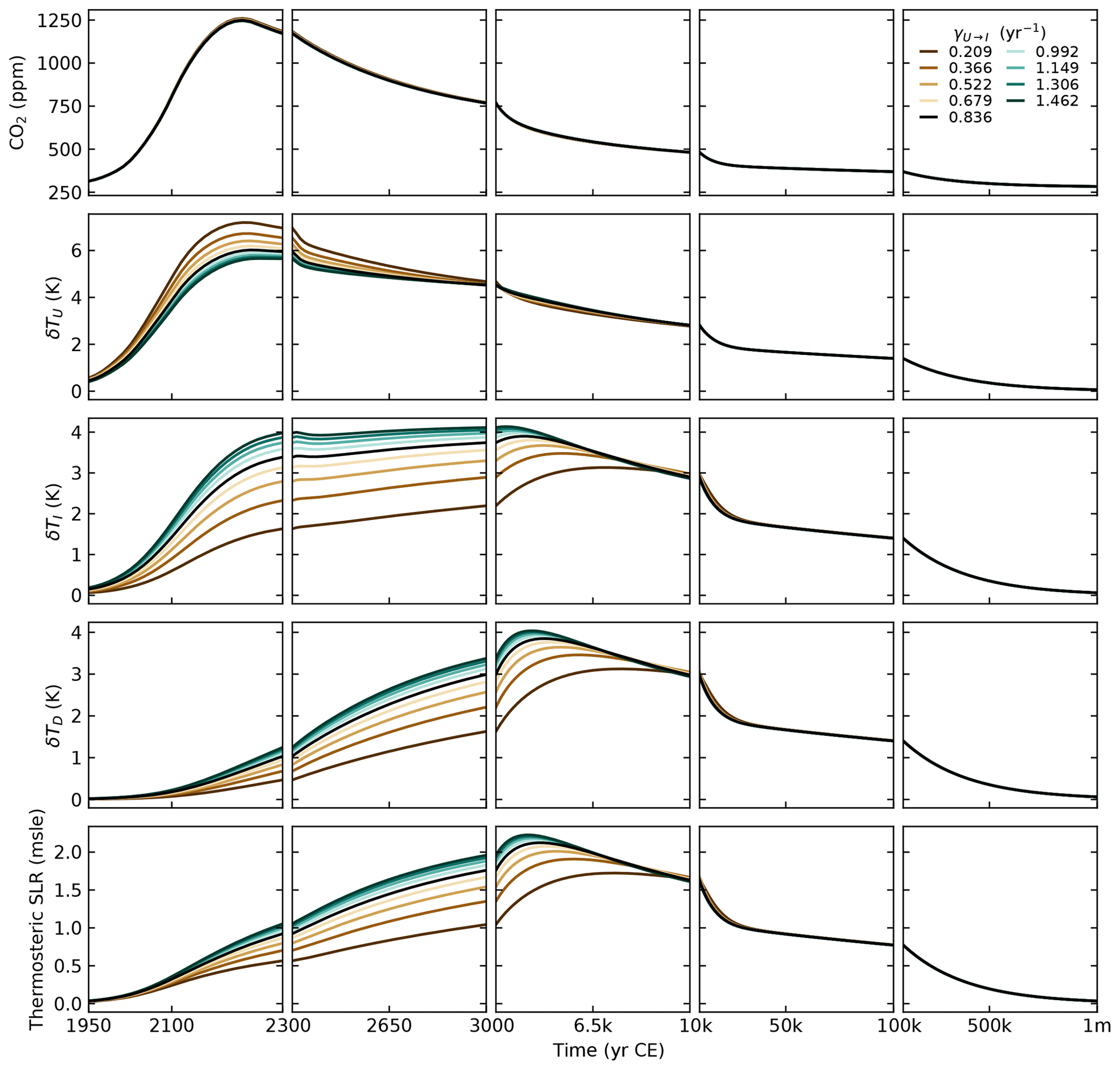
Figure D6 Atmospheric CO₂ concentration, temperatures, and thermosteric sea level rise simulated by SURFER v3.0 under the SSP3-7.0 scenario for different values of γ_U→I. Black lines indicate outputs simulated for the default parameter values, as described in Sect. 2.4.1.

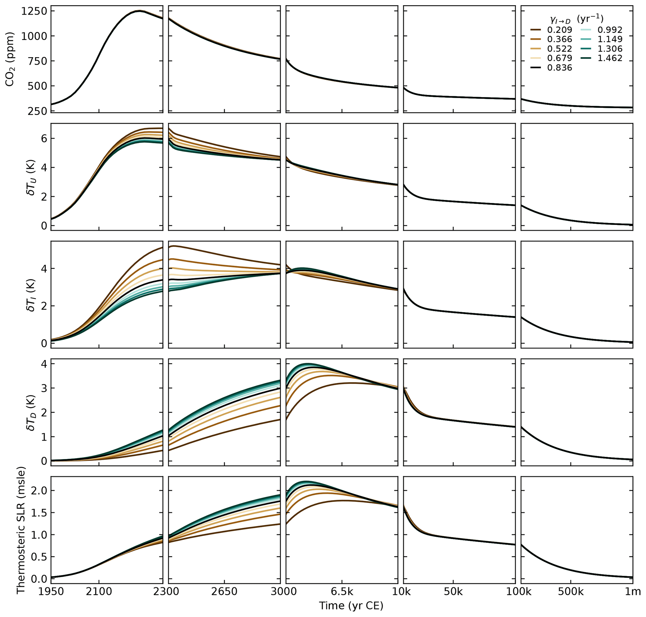
Figure D7 Atmospheric CO₂ concentration, temperatures, and thermosteric sea level rise simulated by SURFER v3.0 under the SSP3-7.0 scenario for different values of γ_I→D. Black lines indicate outputs simulated for the default parameter values, as described in Sect. 2.4.1.

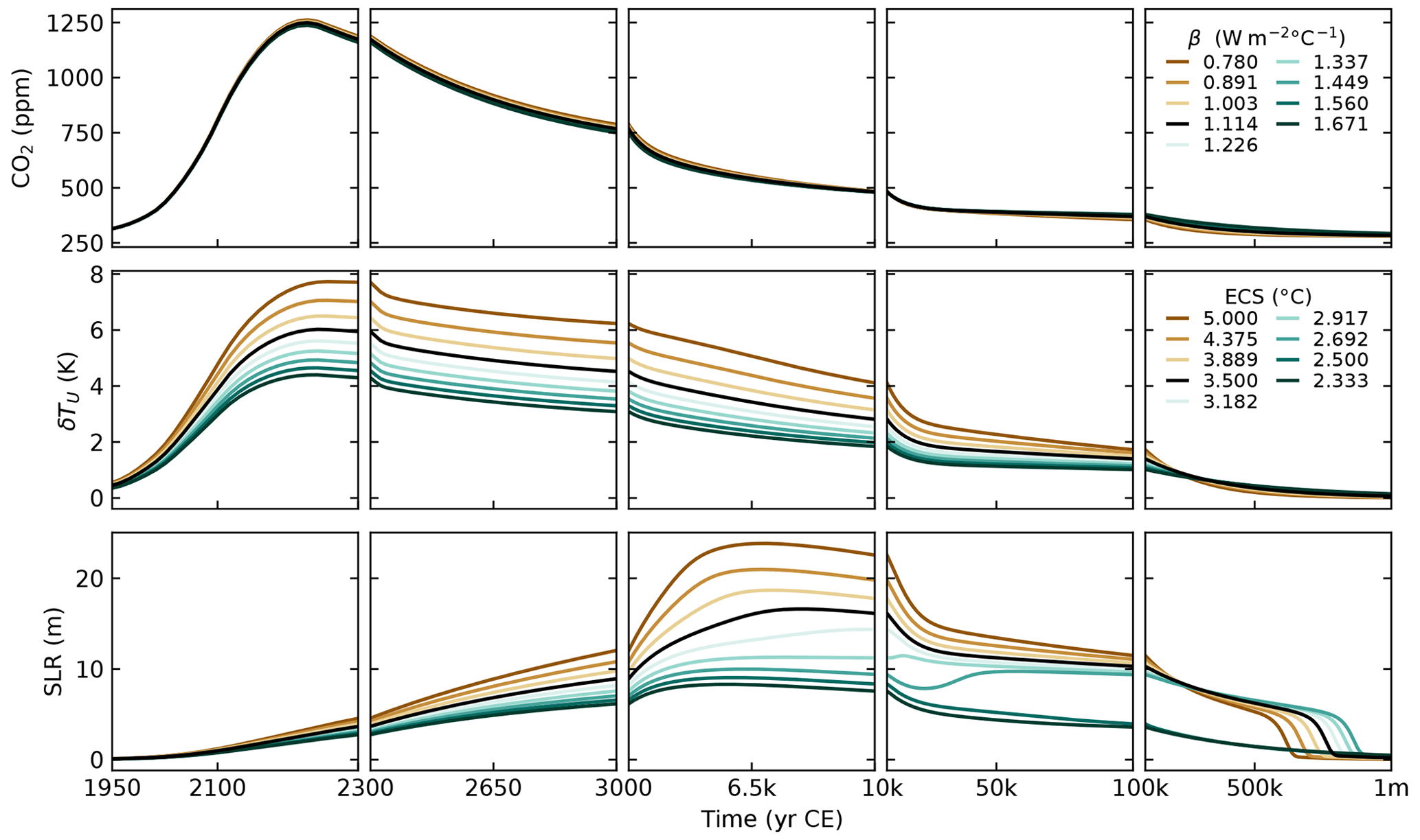
Figure D8 Atmospheric CO₂ concentration, surface temperature, and total sea level rise simulated by SURFER v3.0 under the SSP3-7.0 scenario for different values of β. The equilibrium climate sensitivity of SURFER v3.0 is related to β through $\mathrm{ECS}=F_{\mathrm{2}\times }/\mathit{\beta }$. Black lines indicate outputs simulated for the default parameter values, as described in Sect. 2.4.1.