WRF-ELM v1.0: a regional climate model to study land–atmosphere interactions over heterogeneous land use regions

The Energy Exascale Earth System Model (E3SM) Land Model (ELM) is a state-of-the-art land surface model that simulates the intricate interactions between the terrestrial land surface and other components of the Earth system. Originating from the Community Land Model (CLM) version 4.5, ELM has been under active development, with added new features and functionality, including plant hydraulics, radiation–topography interaction, subsurface multiphase flow, and more explicit land use and management practices. This study integrates ELM v2.1 with the Weather Research and Forecasting (WRF; WRF-ELM) model through a modified Lightweight Infrastructure for Land Atmosphere Coupling (LILAC) framework, enabling affordable high-resolution regional modeling by leveraging ELM's innovative features alongside WRF's diverse atmospheric parameterization options. This framework includes a top-level driver for variable communication between WRF and ELM and Earth System Modeling Framework (ESMF) caps for the WRF atmospheric component and ELM workflow control, encompassing initialization, execution, and finalization. Importantly, this LILAC–ESMF framework demonstrates a more modular approach compared to previous coupling efforts between WRF and land surface models. It maintains the integrity of ELM's source code structure and facilitates the transfer of future developments in ELM to WRF-ELM.

To test the ability of the coupled model to capture land–atmosphere interactions over regions with a variety of land uses and land covers, we conducted high-resolution (4 km) WRF-ELM ensemble simulations over the Great Lakes region (GLR) in the summer of 2018 and systematically compared the results against observations, reanalysis data, and WRF-CTSM (WRF coupled with the Community Terrestrial Systems Model). In general, the coupled WRF-ELM model has reasonably captured the spatial distribution of surface state variables and fluxes across the GLR, particularly over the natural vegetation areas. The evaluation results provide a baseline reference for further improvements in ELM in the regional application of high-resolution weather and climate predictions. Our work serves as an example to the model development community for expanding an advanced land surface model's capability to represent fully-coupled land–atmosphere interactions at fine spatial scales. The development and release of WRF-ELM marks a significant advancement for the ELM user community, providing opportunities for fine-scale regional representation, parameter calibration in coupled mode, and examination of new schemes with atmospheric feedback.

1 Introduction

Land surface models (LSMs) solve the exchange of water, energy, and carbon fluxes between the land surface and atmosphere (Fisher and Koven, 2020) and are frequently used to simulate the response of the Earth's surface to both anthropogenic and natural forcings (Best et al., 2015). These models describe biogeophysical properties like surface roughness, albedo, and evapotranspiration efficiency, characteristics crucial for modeling the land's influence on meteorological processes (Xue et al., 1991; Dai et al., 2003; Dickinson, 1984; Sellers et al., 1986). Originally developed to support weather and climate modeling, LSMs were designed to provide essential lower boundary conditions such as radiation, energy, and water fluxes to the atmosphere.

Over time, LSMs have evolved significantly, with representations of increasingly complex processes that impact land surface dynamics and belowground processes, with their feedback to the atmosphere being incrementally added in newer-generation LSMs. As a consequence of all these advancements, the applicability and scope of LSMs has broadened substantially from their initial versions, introducing sophisticated representations of plant hydraulics (Fang et al., 2022; Xu et al., 2023), wildfire (Thonicke et al., 2010; Li et al., 2012; Huang et al., 2020b, 2021), soil biogeochemistry and nutrient cycling (Li et al., 1992; Parton et al., 1988; Jenkinson, 1990), dynamic vegetation distributions (Martín Belda et al., 2022; Weng et al., 2015; Fisher et al., 2015; Liu et al., 2019), radiation–topography interaction (Hao et al., 2021), urban-scale processes (Oleson and Feddema, 2020; Krayenhoff et al., 2020), subsurface multiphase flow (Bisht et al., 2017; Qiu et al., 2024), and land use and management (Huang et al., 2020a; Binsted et al., 2022; Calvin et al., 2019). These improvements not only advance the capability of LSMs to model complex environmental interactions but also facilitate a mechanistic understanding of changes in land–atmosphere interactions under varying environmental conditions. Particularly, they can be used to predict the disturbance of the land surface, for example Earth's ecosystem and surface hydrology, in response to climate change and to quantify the respective biogeophysical and biogeochemical feedbacks to the climate system (Ban-Weiss et al., 2011; Fisher and Koven, 2020).

Recent advancements in LSMs have broad applications in land-only simulations and within global climate models (GCMs) to capture the complex interactions surrounding global climate change (Lawrence et al., 2019; Martín Belda et al., 2022; Wiltshire et al., 2020). However, the application within GCMs does not allow for the representation of land processes at kilometer scales and extreme events occurring at daily to weekly scales (such as extreme precipitation and flash drought), which are more relevant to human society. While regional refinement may appear to be a feasible solution, the associated computational costs restrict their wide adoption within the weather and climate modeling community. Alternatively, combining advanced LSMs with regional climate models (RCMs) could facilitate more in-depth examinations of the climate change impacts on land surfaces and the resulting feedback at scales that have greater relevance to human society.

The U.S. Department of Energy's Energy Exascale Earth System Model (E3SM) Land Model (ELM) is an advanced LSM that simulates the exchanges between terrestrial land surfaces and other Earth system components, enabling us to understand hydrologic cycles, biogeophysics, and the dynamics of terrestrial ecosystems (Burrows et al., 2020). The Weather Research and Forecasting (WRF) model serves as an essential tool that is widely used for regional weather prediction and climate change analysis (Skamarock and Klemp, 2008). WRF can be run with various LSMs such as Noah, Noah-MP, SSiB, and CLM4. It has also been coupled with the Community Terrestrial Systems Model (CTSM) recently (CTSM Development Team, 2024; UCAR, 2020). However, integrating ELM with WRF enables the comprehensive representation of land processes, following recent advancements in ELM, for more computationally efficient regional modeling applications. For instance, leaf to canopy upscaling through a two-big-leaf parameterization in ELM enables the simulation of the diffuse radiation fertilization effect (Chakraborty et al., 2022) and thus better estimates of surface water and carbon budget, a feature not present in Noah. As another example, ELM incorporates gridwise surface properties such as leaf area index (LAI), displacement height, and vegetation top and bottom height. In contrast, Noah and its variants use lookup tables with these properties prescribed for each land cover class, limiting their ability to capture spatial heterogeneity in surface properties within individual land cover types. Moreover, ELM simulations at ∼ 1 km resolution highlight the significance of considering the radiation–topography interaction in simulating surface energy balance and water budget, a process not yet considered by current land models in WRF (Hao et al., 2021; Yuan et al., 2023).

This study integrates ELM v2.1 with WRF (hereafter named WRF-ELM) using a modified coupler derived from University Corporation for Atmospheric Research's (UCAR) Lightweight Infrastructure for Land Atmosphere Coupling (LILAC) (UCAR, 2020). We evaluate the model performance using a broad range of site observations and reanalysis data, providing a benchmark for subsequent model enhancements. This effort expands the capability of a global LSM, which has been previously used within GCM frameworks, allowing it to simulate higher-resolution land–atmosphere interactions at regional scales. The introduction and release of WRF-ELM also benefit the ELM user community by providing opportunities for them to test new land schemes with atmospheric feedbacks and calibrate model parameters in coupled models.

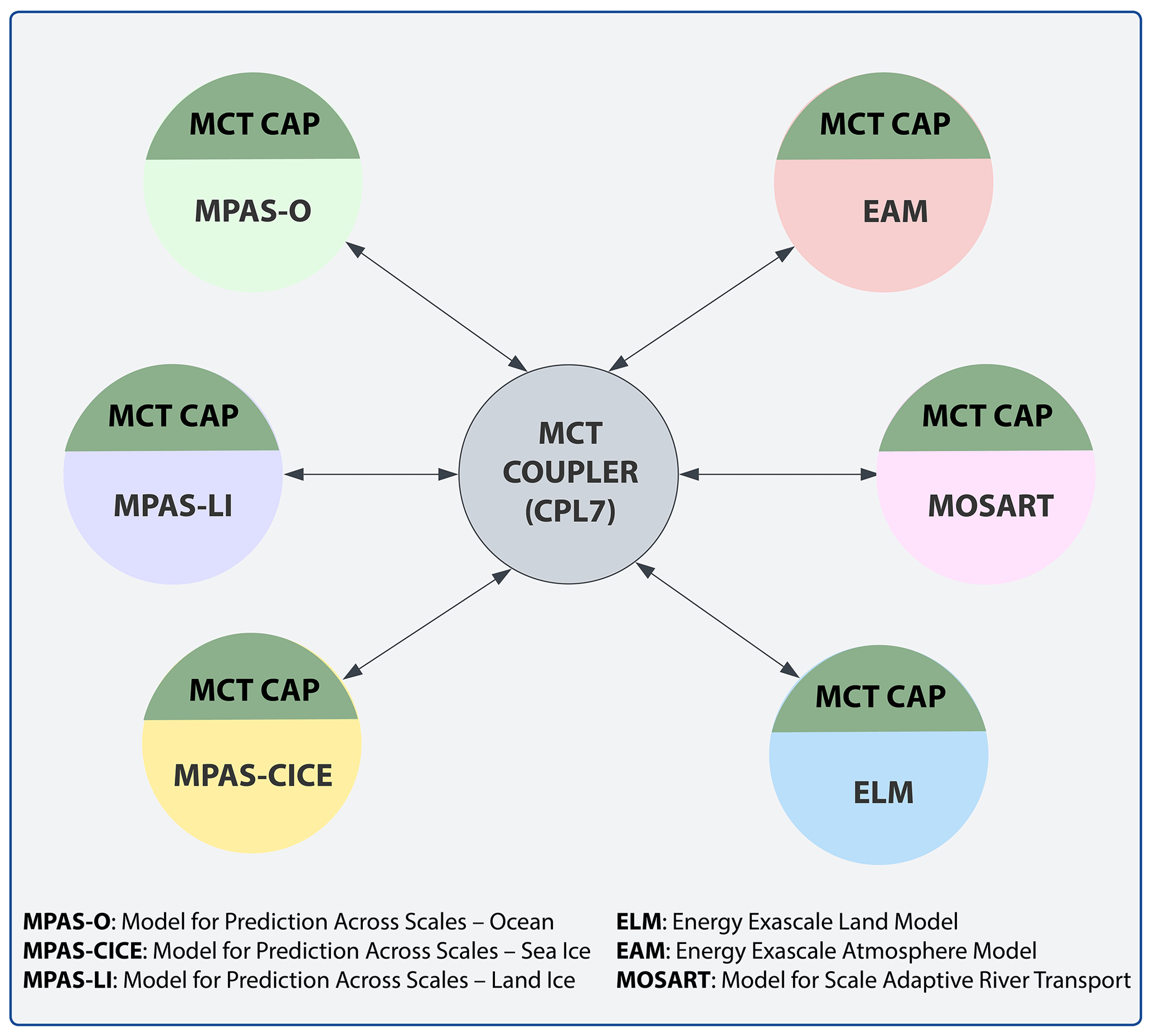
Figure 1 Schematic diagram of the E3SM model components. The top-level coupler (CPL7) serves as the main program for communication between each component. The Model Coupling Toolkit (MCT) cap in each component provides an interface between CPL7 and the physical core, which is responsible for memory allocation, preprocessing, postprocessing, and input and output (I/O).

2 Methods

2.1 Coupler in E3SM

E3SM adopts a hub-and-spoke architecture to couple the different model components together, as shown in Fig. 1. In this architecture, communication between the parallel components is realized via the Model Coupling Toolkit (MCT; Larson et al., 2005; Jacob et al., 2005). The version 7 coupler (CPL7) calls model component initialization, execution, and finalization methods through specified interfaces (Craig et al., 2012). The MCT cap within each component provides an interface between the CPL7 and the physical core, which is responsible for memory allocation, preprocessing, postprocessing, and input and output (I/O). Importantly, the inter-component communication is realized only through the central hub instead of direct communication with one another. The E3SM coupling framework imposes strict requirements on how an atmospheric model can communicate with ELM. One particular challenge is that many atmosphere models – including WRF – expect to run the land model in the middle of the time step sequence. Accomplishing this in the E3SM architecture can require significant restructuring of the atmosphere model. For this reason, ELM has not been coupled to atmospheric models in the regional model community, limiting its ability to address complex scientific challenges at fine resolutions.

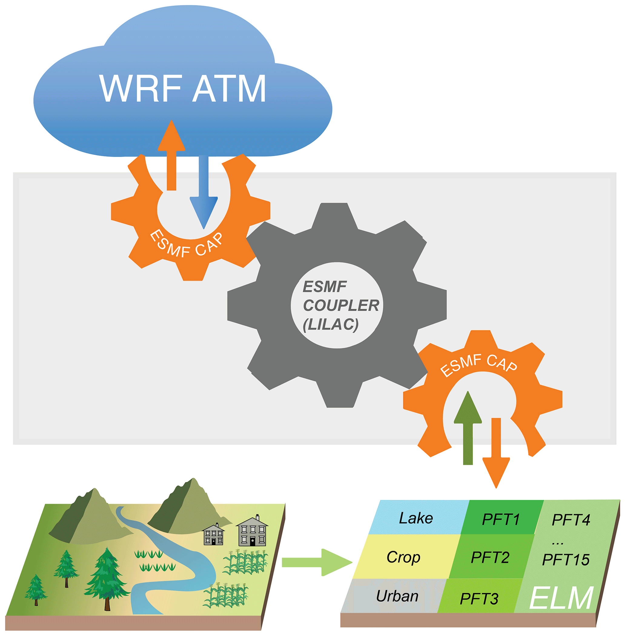
Figure 2 Schematic diagram of the coupling framework for WRF-ELM. The top-level coupler (LILAC) is in charge of communication between WRF ATM and ELM. The ESMF cap within ELM and WRF ATM is responsible for memory allocation, preprocessing, postprocessing, and input and output (I/O). PFT represents plant functional type in the figure.

2.2 LILAC–ESMF (Earth System Modeling Framework) coupler

The traditional way of coupling between LSMs (CLM4, Noah, Noah-MP, and SSiB) and WRF is through internal subroutines and interfaces within the WRF codebase. This tight coupling means that the LSM is often compiled and run as an integral part of the WRF model. As the LSMs grow to integrate more land processes, the tight coupling approach can become less scalable and harder to manage. Additionally, maintaining the coupled system updated with the latest versions of WRF and LSMs can be challenging due to the need for synchronized updates and compatibility checks. In contrast, modern approaches such as LILAC–ESMF offer a more modular and flexible way of coupling, facilitating easier integration and updates of different model components.

We have developed an ESMF (Hill et al., 2004) cap which wraps ELM to facilitate seamless communication with the central hub driver that connects WRF ATM (atmospheric model) and ELM (Fig. 2). The central hub driver, LILAC, is developed using ESMF and provides the fundamental functions to support the integration of an LSM within an RCM, including (1) creating the list of fields passed from WRF ATM to ELM and vice versa; (2) initializing ESMF caps for WRF ATM and for ELM; (3) coordinating calls of the ESMF caps and ELM and exchanging data between these components; and (4) providing missing atmospheric fields, specifically for atmospheric aerosols.

Within the coupling framework, the ESMF cap provides the functions of (1) converting the input data from LILAC to the land model and vice versa; (2) supplying any additional input fields that ELM requires but are not provided by WRF ATM, for example gross domestic product, population density, and lightning that are used to predict fire ignitions in ELM; and (3) setting the domain decomposition and generating the land mesh. The ESMF cap, which provides the necessary infrastructure to connect LILAC and ELM physics, serves as an example for similar coupling work between other LSMs and RCMs.

2.3 Exchange variables between WRF and ELM

ELM is driven by meteorological forcings including precipitation, downward shortwave radiation, downward longwave radiation, zonal wind at reference height (z_atm), meridional wind at z_atm, pressure at z_atm, specific humidity at z_atm, and air temperature at z_atm. In the coupled version, the meteorological forcings are provided by WRF ATM with the ELM model time step set to match the integration time step in the WRF ATM. The reference height refers to the height of the lowest atmosphere model level. The radiation scheme in WRF further splits the shortwave radiation to direct and diffuse components, as well as visible and near-infrared radiation. Precipitation is divided into rainfall and snowfall based on the frozen precipitation ratio, which are then inputted into ELM. The ELM output includes skin temperature, 2 m air temperature, 2 m specific humidity at the surface, friction velocity, surface albedo, sensible heat flux, latent heat flux, ground heat flux, surface emissivity, and roughness length for momentum and heat transfer, which will be exchanged with the WRF ATM component.

2.4 Mesh data and surface parameters

In addition, mesh data are used in the WRF ATM to define the latitude and longitude of the grid. The domain information is necessary for the coupler and the land model during runtime. These data include a mask that informs the land model where to run and a land fraction that the coupler uses to combine fluxes from various surface types over a grid cell. The surface data configure the spatially implicit features (e.g., spatial fraction coverage, leaf and soil albedo, leaf and soil emissivity) of subgrid elements within grid cells (topographic unit, land cover, soil columns, and vegetation).

While a regular latitude–longitude grid is widely used for domain and surface data in the land-only mode, when coupled with WRF ATM, ELM needs to adopt the Lambert conformal projection used in WRF. To create a domain file of Lambert conformal projection, a grid descriptor file based on the WRF Pre-Processing System (WPS) output (e.g., geo_em.d01) needs to be created, which is then used to create the domain file used in ELM. A similar workflow is needed for surface data, which contain a large number of input files that need to be interpolated by the land model. To generate both domain files and surface data, we employ the ELM preprocessing tools that derive the input data and grid descriptor files for each dataset, produce mapping files from the input data grid to our target grid, and then use the mapping weight files for interpolation.

Figure 3 Schematic of the parallel domain decomposition scheme in WRF-ELM. The dotted area indicates “halo” arrays in which memory is shared between processors (P0 and P1). WRF ATM and ELM are calculated using the same processor.

2.5 Parallelization

Instead of adopting ELM's native round-robin domain decomposition strategy, our parallelization strategy for WRF-ELM is to use geographic domain decomposition, like in WRF ATM. As shown in Fig. 3, different grid cells in the model's physical domain are running on separate processors preassigned by the user. On each processor, ELM within WRF employs parallel I/O to read atmospheric forcings, uses the surface properties and land use datasets to configure individual land cells, and then conducts massively parallel simulations over these grid cells within each subdomain independently. In WRF ATM, the “halo” arrays share memory between processors, and message passing between processors is accomplished using the message passing interface (MPI; Gropp et al., 1996).

3 Model validation

3.1 WRF-ELM configuration

For our first WRF-ELM application, we study the land–atmosphere interactions over the Great Lakes region (GLR), a hydrodynamically complex and heavily populated region with both natural surface heterogeneity and significant land management practices. This domain also includes the world's largest freshwater system, comprising lakes Superior, Michigan, Huron, Erie, and Ontario. This region is the focus of the U.S. Department of Energy's (DOE) Coastal Observations, Mechanisms, and Predictions Across Systems and Scales, Great Lakes Modeling (COMPASS-GLM) project, which has an overall goal of developing a fully coupled (lake–land–atmosphere) regional earth system model centered on the GLR (Kayastha et al., 2023). Here, we report the initial implementation of the WRF-ELM framework to support its ability to capture atmospheric, coastal, urban, and rural interactions, providing a baseline reference solution for further model development.

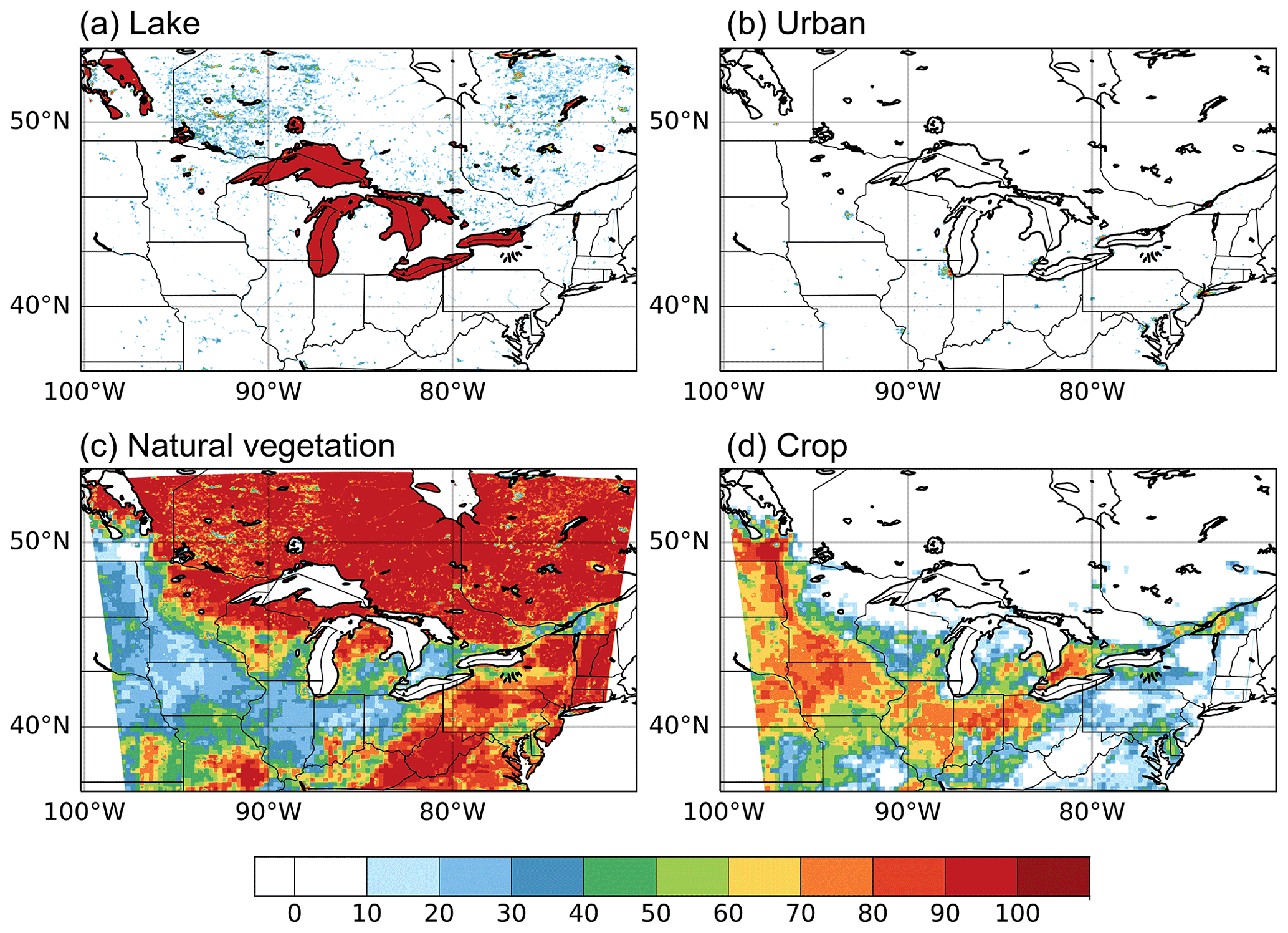
Figure 4 Fractional coverage (%) of the major land units used in WRF-ELM: (a) lake, (b) urban, (c) natural vegetation, and (d) crop.

The RCM used in the numerical simulation is based on WRF model version 4.4.2 with the Advanced Research WRF dynamic core (Skamarock and Klemp, 2008). Following Wang et al. (2022a), the model domain is centered at 45.5° N and 85.0° W and has dimensions of 544 × 485 grid points in the west–east and south–north directions. The simulation domain covers the GLR, with a spatial resolution of 4 km (Fig. 4). The 50 vertical layers from the surface to 50 hPa are adopted with denser layers at lower altitudes to sufficiently resolve the planetary boundary layer (PBL). We conduct five ensemble members in 2018, starting with initial conditions 12 h apart between 00:00 UTC on 12 May and 00:00 UTC on 14 May and ending at 00:00 UTC on 1 September 2018. The resulting simulations are analyzed during June, July, and August (JJA) 2018.

Table 1 Model configuration in WRF and ELM.

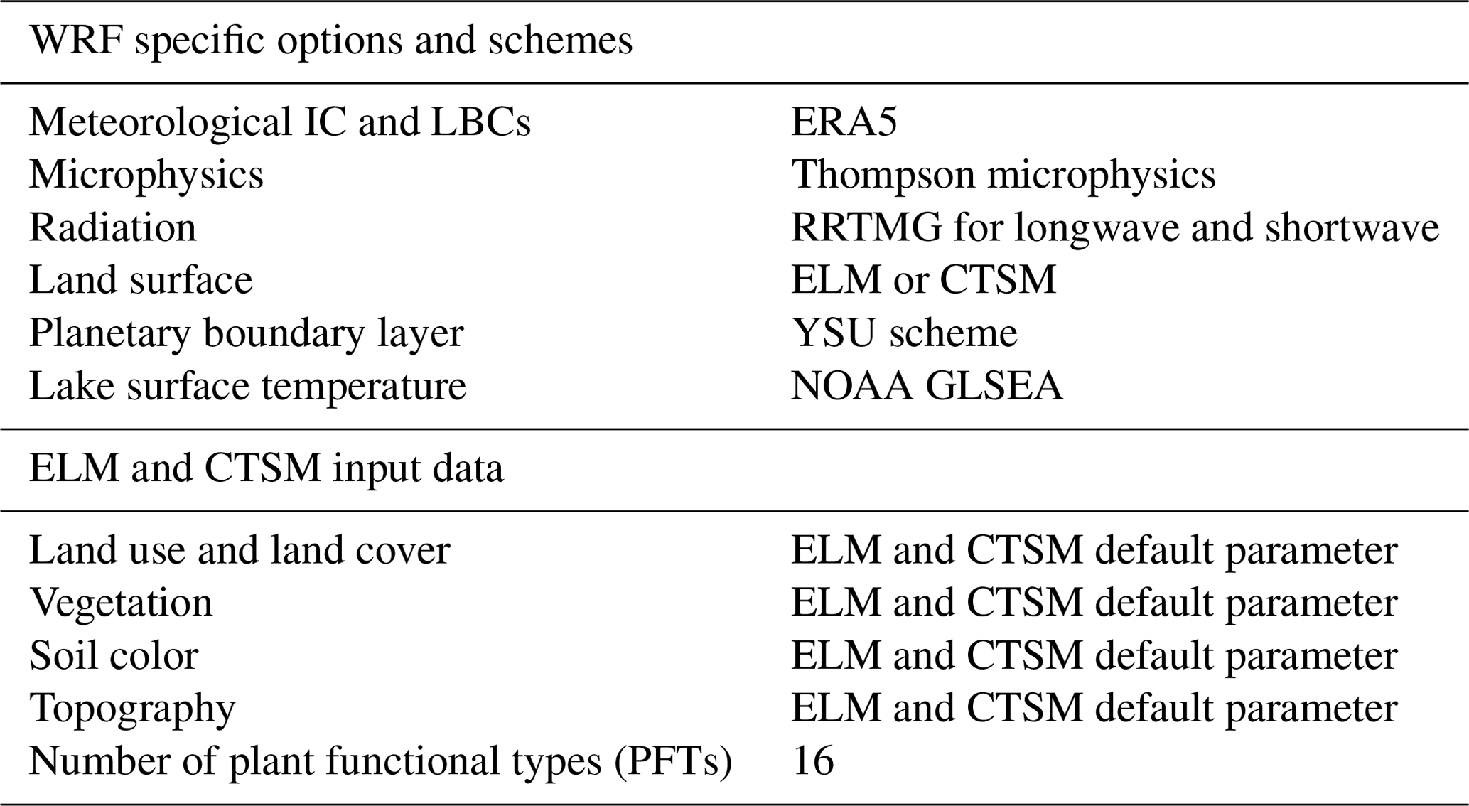
The meteorological initial condition (IC) and lateral boundary conditions (LBCs) have been derived from ECMWF Reanalysis v5 (ERA5; Hersbach et al., 2020) at 0.25° horizontal resolution and 3 h temporal intervals (Table 1). The WRF model incorporates Thompson microphysics (Thompson et al., 2004, 2008), the Rapid Radiative Transfer Model for GCMs (RRTMG) longwave and shortwave radiation schemes (Iacono et al., 2008), and the Yonsei University (YSU) planetary boundary layer scheme (Hong and Lim, 2006). We turn off cumulus parameterization, considering the convection-permitting resolution of the ensemble simulations. The lake skin temperature is obtained from the NOAA Great Lakes Surface Environmental Analysis (GLSEA) data set (Schwab et al., 1992) derived from an advanced, very high-resolution radiometer.

For the land surface model, we adopt the ELM with satellite phenology (ELM-SP) mode which utilizes the seasonally varying leaf area index prescribed based on the MODIS data. The default ELM land surface parameters have been used in the coupled model simulation, including land use and land cover information, vegetation biogeophysical properties, soil properties, and topography. The surface parameter is also applicable in CTSM (Table 1). A detailed description of the ELM and CTSM default parameter can be found in Li et al. (2024). The current version of WRF-ELM does not enable the biogeochemistry (ELM-BGC) mode and thus does not simulate carbon and nitrogen cycles. In addition, we also conduct simulations using the WRF coupled with Community Terrestrial Systems Model (CTSM ctsm5.1.dev114) (Lawrence et al., 2019) (WRF-CTSM hereafter), which can be compared with WRF-ELM's performance in capturing the land–atmosphere exchanges of energy and water fluxes. CTSM is also referred to as the Community Land Model version 5 (CLM5) afterwards. We emphasize that the comparison against WRF-CTSM is not intended to demonstrate the superior performance of WRF-ELM but to show that the newly developed WRF-ELM performs comparably well to WRF-CTSM, one of the most advanced and sophisticated land surface models.

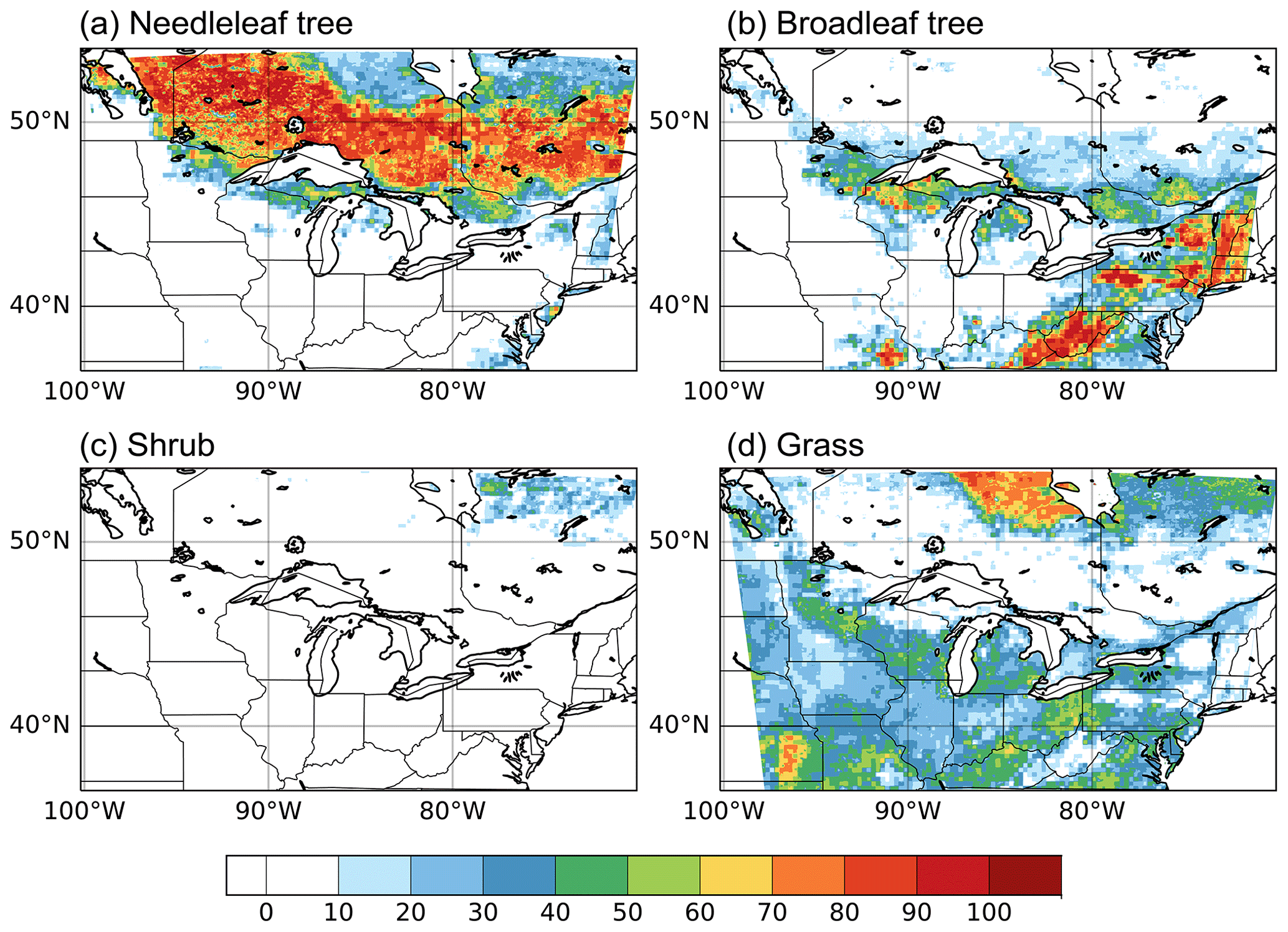
Figure 5 Fractional coverage (%) of the major plant functional types used in WRF-ELM: (a) needleleaf forest (deciduous and evergreen combined), (b) broadleaf forest (deciduous and evergreen combined), (c) shrub, and (d) grass.

It is noteworthy that there are several distinctions between WRF-ELM and the version of WRF-CTSM we use here. WRF-CTSM aims for a relatively fast calculation speed; thus it has simplified the description of land cover and kept the single dominant land unit and single dominant plant functional types (PFTs). In our simulation region, WRF-CTSM identifies the Great Lakes in the center of the simulation domain, with the natural vegetation prevailing in the northern and southeastern regions and crops dominating the southwestern areas (Fig. 4). On the other hand, WRF-ELM preserves the comprehensive description of subgrid heterogeneity. As a result, the fluxes calculated from various surface types are merged using a weighted-average method before transferring to the upper-level WRF ATM. This is particularly important in regions with mixed vegetation types, such as the southwestern part of our study domain. Moreover, within the natural vegetation land unit, WRF-ELM simulates the blend of needleleaf and broadleaf trees (evergreen and deciduous combined) around the Great Lakes and the mixture of crops and grasses in the southwestern part of the domain (Fig. 5).

Table 2 Dataset for validation in the study.

3.2 Data for validation

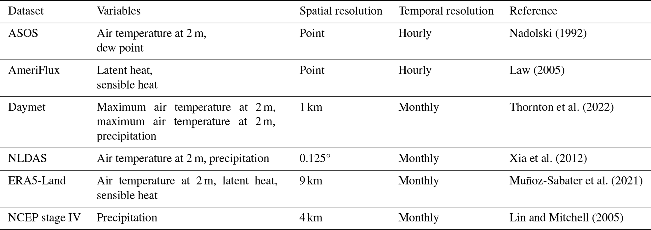
Observational and reanalysis data from multiple sources have been used to evaluate WRF simulation results (Table 2). We select 12 paired sites from the Automated Surface Observing System (ASOS) to acquire 5 min 2 m air temperature (T_a) and 2 m dew point temperature over the urban and rural area in the GLR (https://www.ncei.noaa.gov, last access: November 2023). The 2 m relative humidity (RH) is derived from T_a and dew point. We compute hourly averages of T_a and RH from the 5 min data to match the hourly WRF outputs.

Table 3 AmeriFlux site information (LCF: land cover type; DBF: deciduous broadleaf tree; MF: mixed forest; PI: principal investigator; NEON: National Ecological Observatory Network).

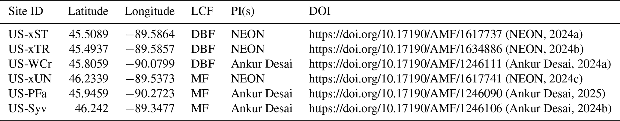
In addition, we collect measurements of latent heat (LH) and sensible heat (SH) from six flux tower sites provided by AmeriFlux (http://ameriflux.lbl.gov, last access: November 2023). Initially, 16 AmeriFlux sites had been selected within our study domain for the JJA 2018 period, which included measurements over grassland, mixed forest, and deciduous broadleaf forest. However, 10 sites are filtered out because their land cover types differ from the dominant ones used in WRF-CTSM. The latitudes and longitudes of selected sites have been documented in Table 3. The hourly LH and SH data from AmeriFlux have been reduced to daily averages to validate the model simulation of surface energy fluxes.

We also acquire reanalysis datasets to evaluate the model performance in simulating the climate variables and energy fluxes. All datasets are resampled using bilinear interpolation to a 4 km resolution to align with the WRF grids. We employ the Daymet dataset from https://daymet.ornl.gov (last access: October 2023), which provides daily, gridded (1 km × 1 km) estimates of solar radiation, 2 m maximum (T_max) and minimum (T_min) temperature, precipitation (PRE), snow water equivalent, and water vapor across the contiguous United States (CONUS; Thornton et al., 2022). It uses local regression algorithms to interpolate and extrapolate daily meteorological observations from the Global Historical Climatology Network (GHCN). Daymet considers the effects of elevation on climate and generates daily meteorological variables for a particular grid cell using the weighted-linear-regression-based approach. We download monthly T_max, T_min, and precipitation from Daymet version 4.5 and average the temperatures to compare against model-simulated daily mean T_a.

Monthly T_a from the North American Land Data Assimilation System (NLDAS) version 2 with Noah LSM is used as an additional source of reanalysis data to evaluate WRF-ELM. These data are available beginning in 1979 at a 0.125° resolution (Xia et al., 2012). NLDAS constructed a forcing dataset from a daily gauge-based precipitation analysis, bias-corrected shortwave radiation, and surface meteorology reanalyses from the North American Regional Reanalysis (NARR) to drive four different LSMs to derive surface fluxes and state variables. We acquire the product derived using the Noah model (https://disc.gsfc.nasa.gov, last access: October 2023) because it is one of the most commonly used LSMs and has been frequently coupled with climate and atmospheric models.

The ERA5-Land reanalysis provides surface variables at 0.1° × 0.1° resolution (Muñoz-Sabater, 2019). The data are produced under the offline mode forced by meteorological fields from ERA5 (Muñoz-Sabater et al., 2021) without coupling to the atmospheric module of the ECMWF's Integrated Forecasting System. ERA5-Land datasets have also been widely used for a variety of land condition assessments (Pelosi et al., 2020; Stefanidis et al., 2021; Wang et al., 2022b). We acquire monthly T_a, SH, and LH in ERA5-Land from Google Earth Engine (collection ECMWF/ERA5_LAND/MONTHLY_AGGR; last access: October 2023).

Lastly, we acquire precipitation data from the National Centers for Environmental Prediction (NCEP) stage IV dataset (Lin and Mitchell, 2005), a gridded product with 4 km spatial resolution and hourly temporal resolution that covers the period from 2002 to the present. NCEP compiles the stage IV product using data from 140 radars and approximately 5500 gauges across the CONUS. The Stage IV product provides highly accurate precipitation estimates, particularly for medium to heavy precipitation, and has therefore been widely used as a reference for precipitation evaluation (Nelson et al., 2016).

Figure 6 June–July–August mean 2 m air temperature (K) in (a) WRF-ELM, (b) WRF-CTSM, (c) Daymet, (d) NLDAS, and (e) ERA-Land.

Table 4 Evaluation metrics of June–July–August 2 m air temperature between each model result and the reanalysis product. CORR: spatial correlation coefficient; RMSE: root mean square error.

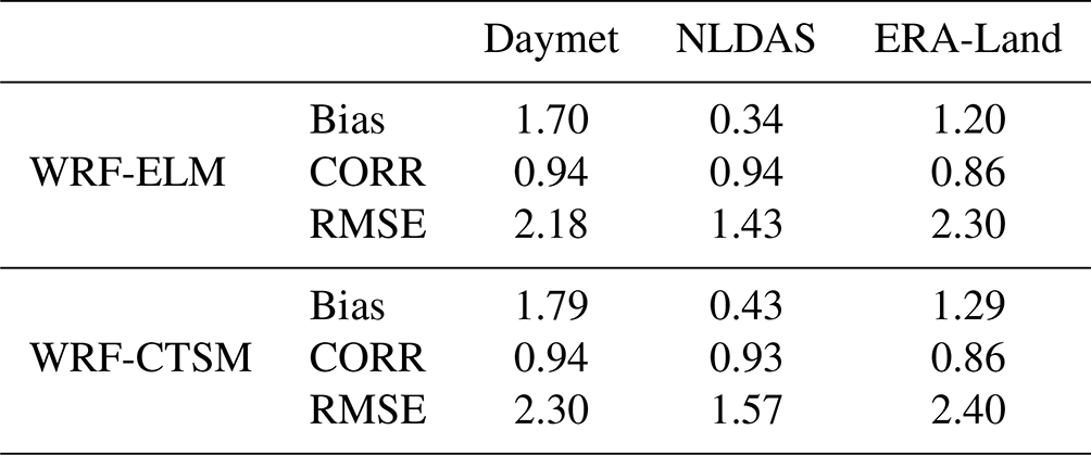
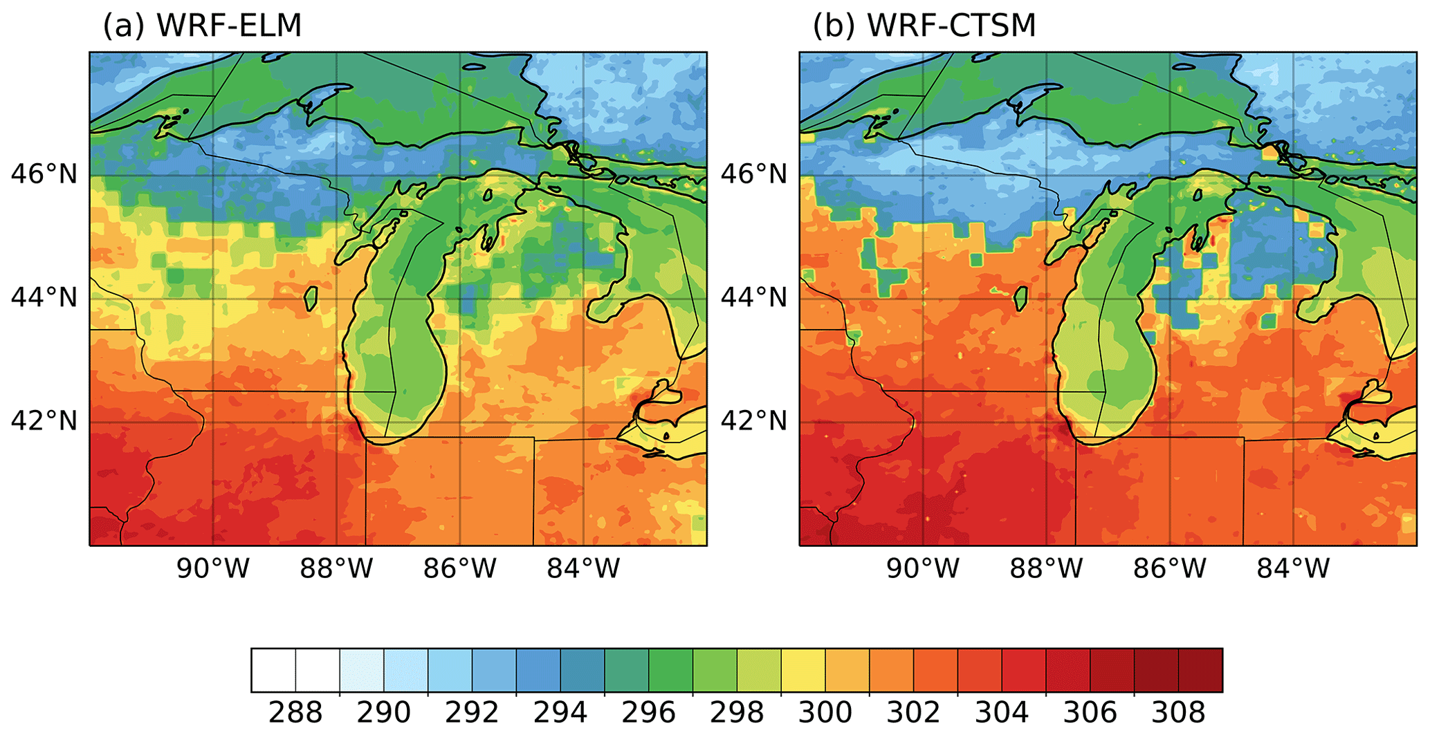
Figure 7 June–July–August mean skin temperature (K) in (a) WRF-ELM and (b) WRF-CTSM; the zoomed-in view focuses on the area surrounding Lake Michigan.

3.3 Results

3.3.1 Temperature

The spatial distribution of T_a from the WRF-ELM and WRF-CTSM models, along with reanalysis data such as Daymet, NLDAS, and ERA5-Land, is illustrated in Fig. 6. Both WRF-ELM and WRF-CTSM have reasonably captured the spatial pattern observed in the reanalysis datasets, demonstrating a spatial correlation coefficient (CORR) ranging from 0.86 to 0.95 (Table 4). The highest CORR is observed with Daymet, while the lowest one is with ERA5-Land. Both models exhibit a warm bias compared to reanalysis products. However, WRF-ELM shows a slightly lower bias and RMSE compared with WRF-CTSM (Table 4). Additionally, WRF-ELM displays a smoother gradient in comparison to WRF-CTSM, particularly over the GLR where needleleaf trees, broadleaf trees, grasses, and croplands coexist (Fig. 7).

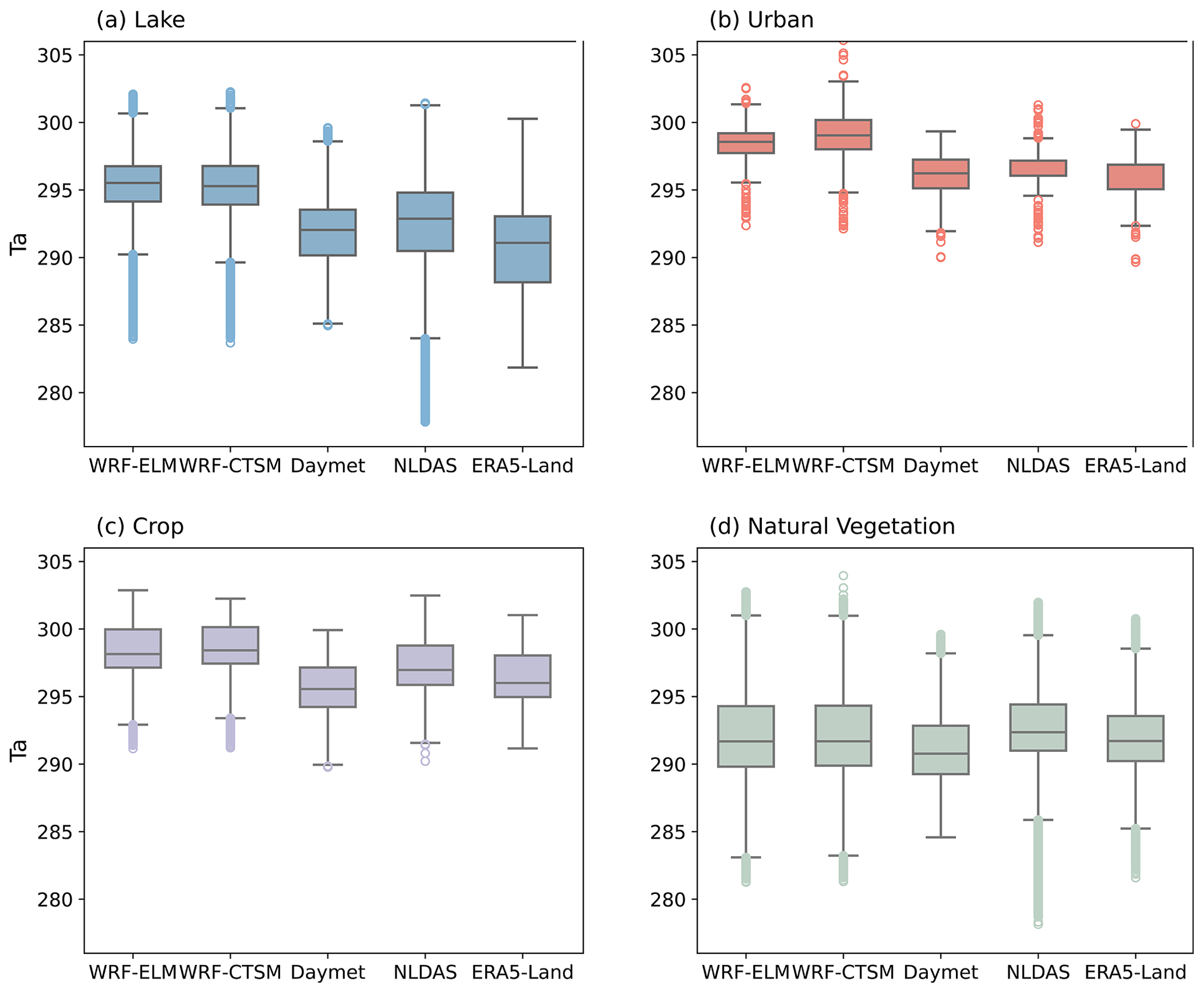
Figure 8 Boxplots of June–July–August 2 m air temperature (K) over (a) lake, (b) urban, (c) crop, and (d) natural vegetation in simulations and reanalysis products.

Table 5 June–July–August 2 m air temperature over each land unit in simulations and reanalyses.

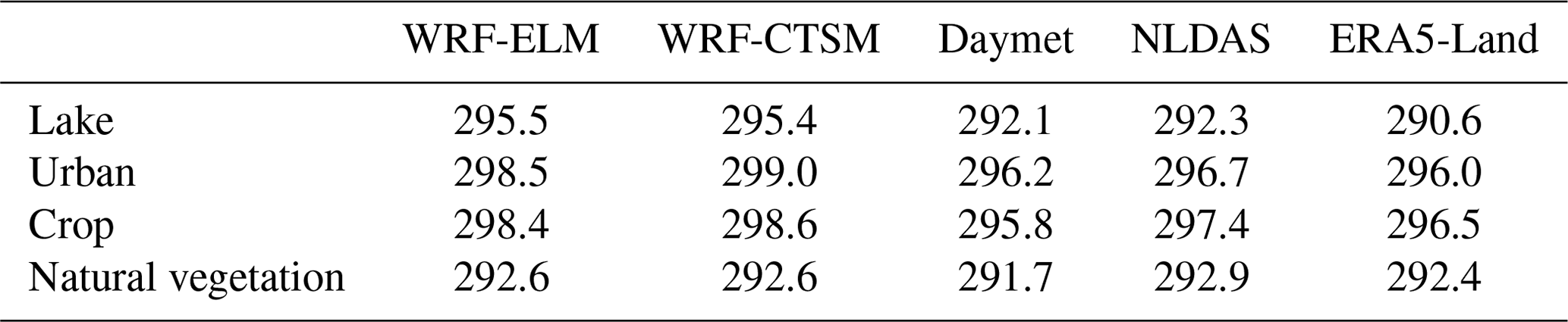
Despite the overall good performance of the model simulation of T_a, it is slightly different among different land units (Fig. 8). The largest warm bias is found over the lake surface, in which both models have overestimated T_a by 3–5 K (Table 5, Fig. 8). For urban and crop areas, WRF-ELM and WRF-CTSM show a slightly warmer temperature by 2–3 K than all reanalysis data, which makes sense since reanalysis datasets do not capture urban-scale warming signals (Chen et al., 2024). The T_a over the natural vegetation is well captured, with the average value in both models within the range of average T_a over all datasets.

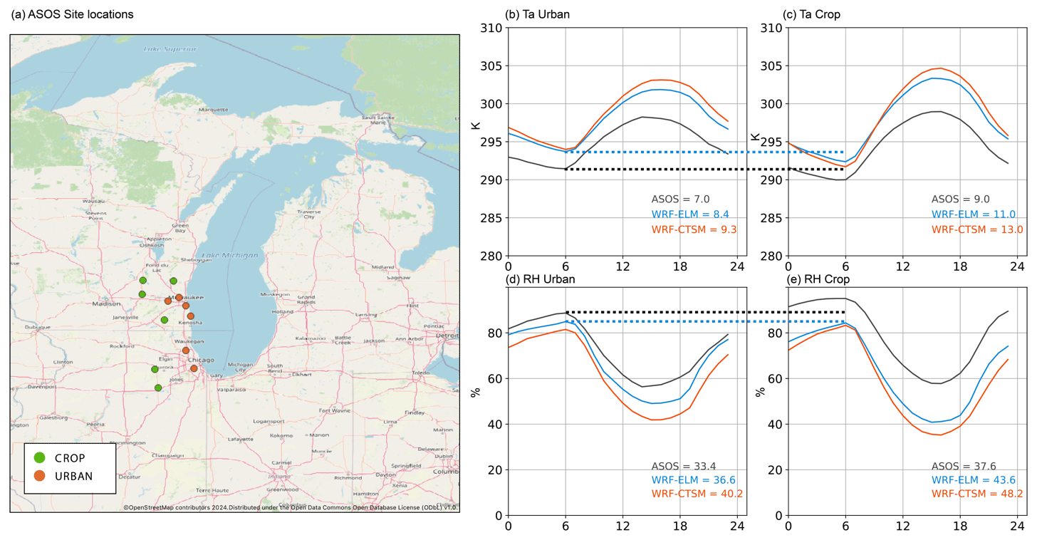
Figure 9 (a) The location of ASOS sites. (b–c) June–July–August hourly-averaged 2 m air temperature over (b) urban and (c) crop land units for ASOS, WRF-ELM, and WRF-CTSM. (d–e) The same as (b)–(c) but for 2 m relative humidity. The numbers in (b)–(e) indicate the diurnal ranges of air temperature and relative humidity from ASOS, WRF-ELM, and WRF-CTSM. The dashed lines highlight the nighttime T_a and RH when urban and crop contrasts are significant.

We use ASOS sites to investigate the representation of urban and lake effects on air temperature and relative humidity over the metropolitan area, emphasizing the interaction between the urban heat island (UHI; Rizwan et al., 2008) and lake breeze in WRF-ELM and WRF-CTSM. Six urban sites along the west coast of Lake Michigan were selected, paired with six adjacent crop sites as reference points (Fig. 9a). Compared to the rural crop sites, the urban sites exhibit higher minimum T_a during the night, as urban areas retain more heat during the daytime and gradually release it after sunset. During late morning to noon, the lake breeze tends to cool urban air, resulting in a lower daily maximum T_a than observed in crop areas (Wang et al., 2023). In the afternoon, urban sites show a more gradual decline in T_a compared to rural sites, driven by the cumulative heating effect of solar radiation absorption and the heat release by urban materials throughout the day (Soltani and Sharifi, 2017). This characteristic of urban areas leads to a smaller diurnal temperature range of 7.0 K, compared to a 9.0 K range over crop sites (Fig. 9b–c). The urban dry island (UDI) effect is also evident in 2 m RH observations from ASOS, with urban areas showing lower RH values at night (Fig. 9d–e).

Both WRF-ELM and WRF-CTSM capture the warmer nighttime T_a due to the UHI effect and the cooler daytime T_a caused by the lake breeze over urban sites, adequately reproducing the smaller diurnal range. WRF simulations, particularly WRF-ELM, reasonably capture urban RH at night, but both models underestimate RH over crop areas, so the UDI is not well captured in the simulations. Notably, WRF-ELM generally exhibits smaller biases in both T_a and RH compared to WRF-CTSM (Fig. 9). However, both models systematically overestimate T2 and underestimate RH in both urban and crop areas, suggesting a persistent warm and dry bias needs to be further investigated in the ELM and CTSM component.

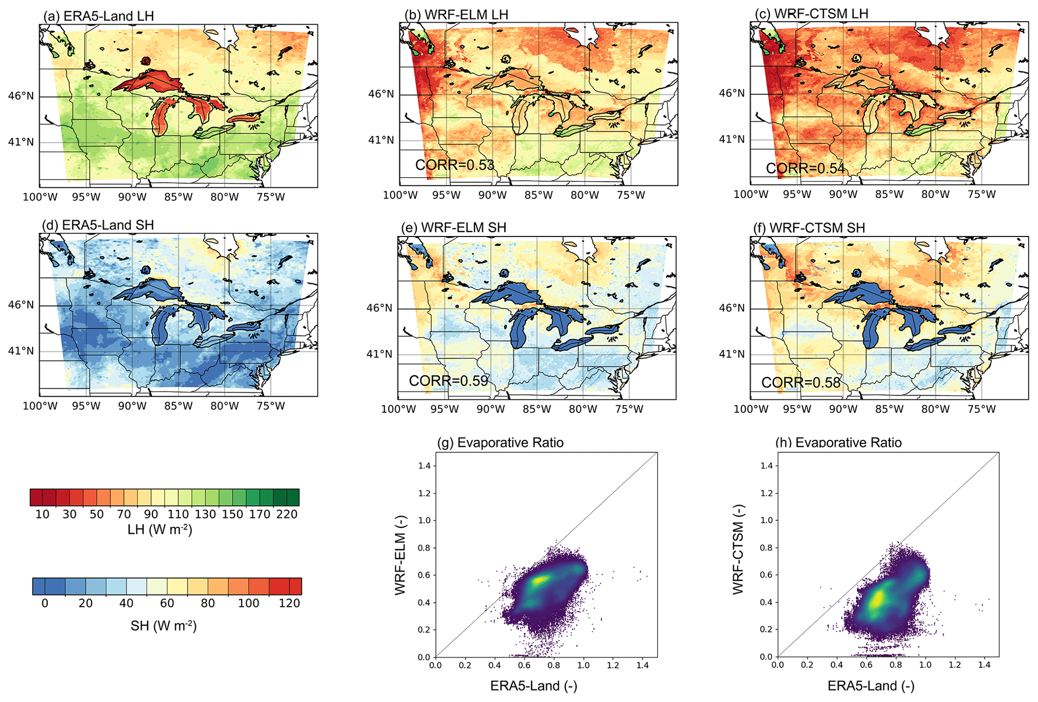
Figure 10 (a–c) Spatial distribution of latent heat in (a) ERA5-Land, (b) WRF-ELM, and (c) WRF-CTSM. (d–f) Spatial distribution of sensible heat in (d) ERA5-Land, (e) WRF-ELM, and (f) WRF-CTSM. (g–h) Comparison of evaporative ratio between (g) WRF-ELM and ERA5-Land and (h) WRF-CTSM and ERA5-Land over the natural vegetation grids.

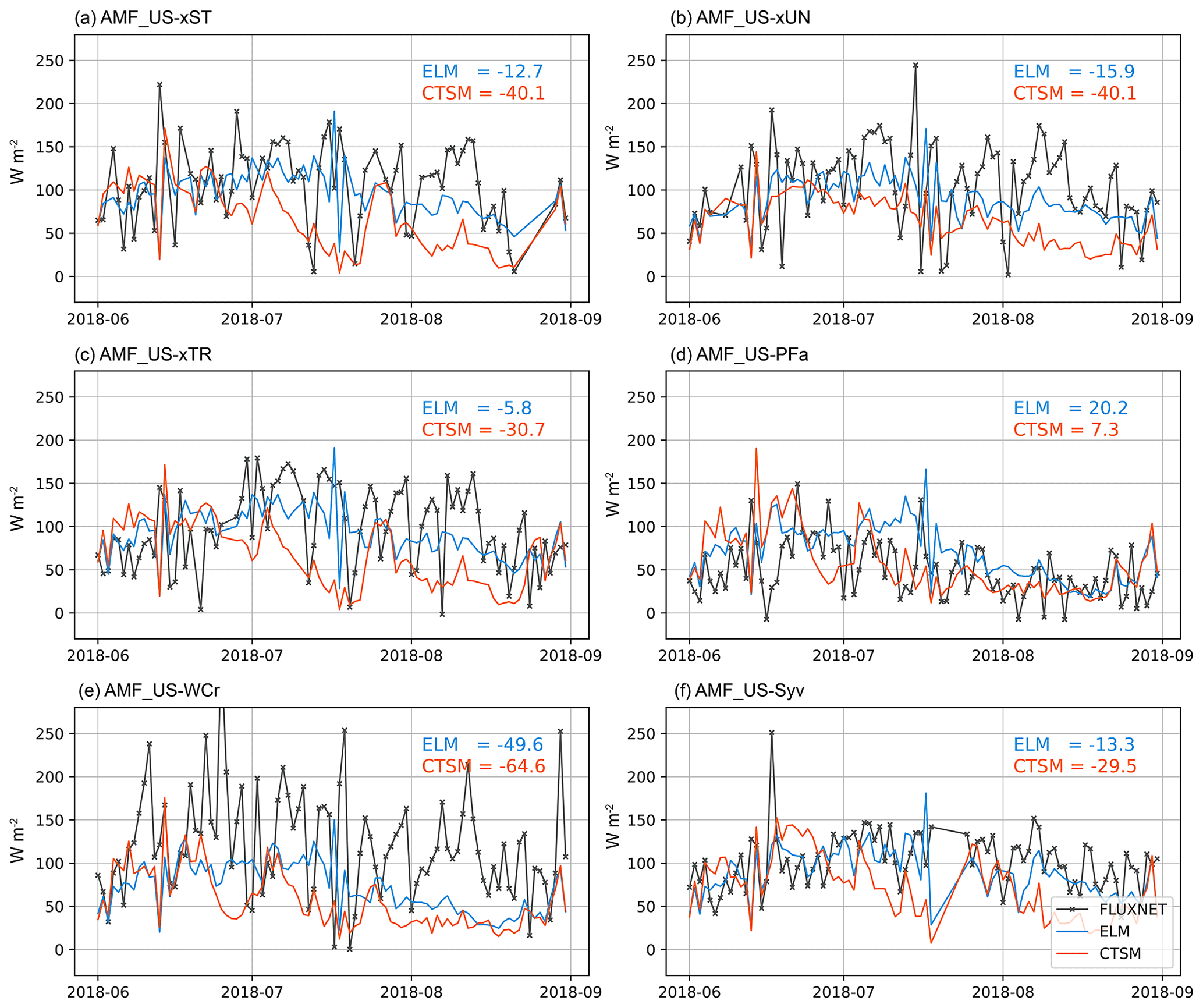
Figure 11 June–July–August daily-averaged LH fluxes from six AmeriFlux sites and the corresponding model grids. The numbers indicate biases between WRF-ELM (or WRF-CTSM) and AmeriFlux.

3.3.2 Energy fluxes

We evaluated the simulated LH and SH fluxes from the WRF model simulations against ERA5-Land reanalysis data. The spatial correlation coefficient (CORR) values range from 0.53 to 0.58 (Fig. 10a–f). Overall, both models capture the LH gradient across the study domain, with higher LH observed in the southern region and lower LH in the northern region. Similarly, both the reanalysis data and the models show a higher SH in the northern region and lower SH in the south. A systematic underestimation of LH (ranging between 22–35 W m⁻²) and overestimation of SH (averaging 21–31 W m⁻²) are evident in both WRF-ELM and WRF-CTSM. The observed evaporative fraction ranges from 0.6 to 0.8 in most vegetated grids; however, the corresponding simulated evaporative fraction is approximately 0.6. This evaluation further confirms that our models tend to underestimate LH fluxes while overestimating SH fluxes. These biases may be largely attributed to the surface parameter uncertainties used in the current simulations, such as LAI or roughness length. These parameters have not been thoroughly calibrated in coupled E3SM simulations focusing on the Great Lakes region.

A further comparison of daily LH values from six AmeriFlux sites over deciduous broadleaf forests is illustrated in Fig. 11. WRF-ELM exhibits a smaller bias in reproducing the magnitude of LH than WRF-CTSM; however, neither model captures the temporal variations well. Comparing regional model simulations with site-level observations remains a consistent difficulty due to the inherent scale mismatch between point observations and grid-based simulations. Additionally, since we examined a relatively short period without interannual variability or seasonal cycles, the temporal variations in surface energy are mostly related to the simulation of cloud and precipitation variations, which are among the most uncertain parts of regional climate simulations.

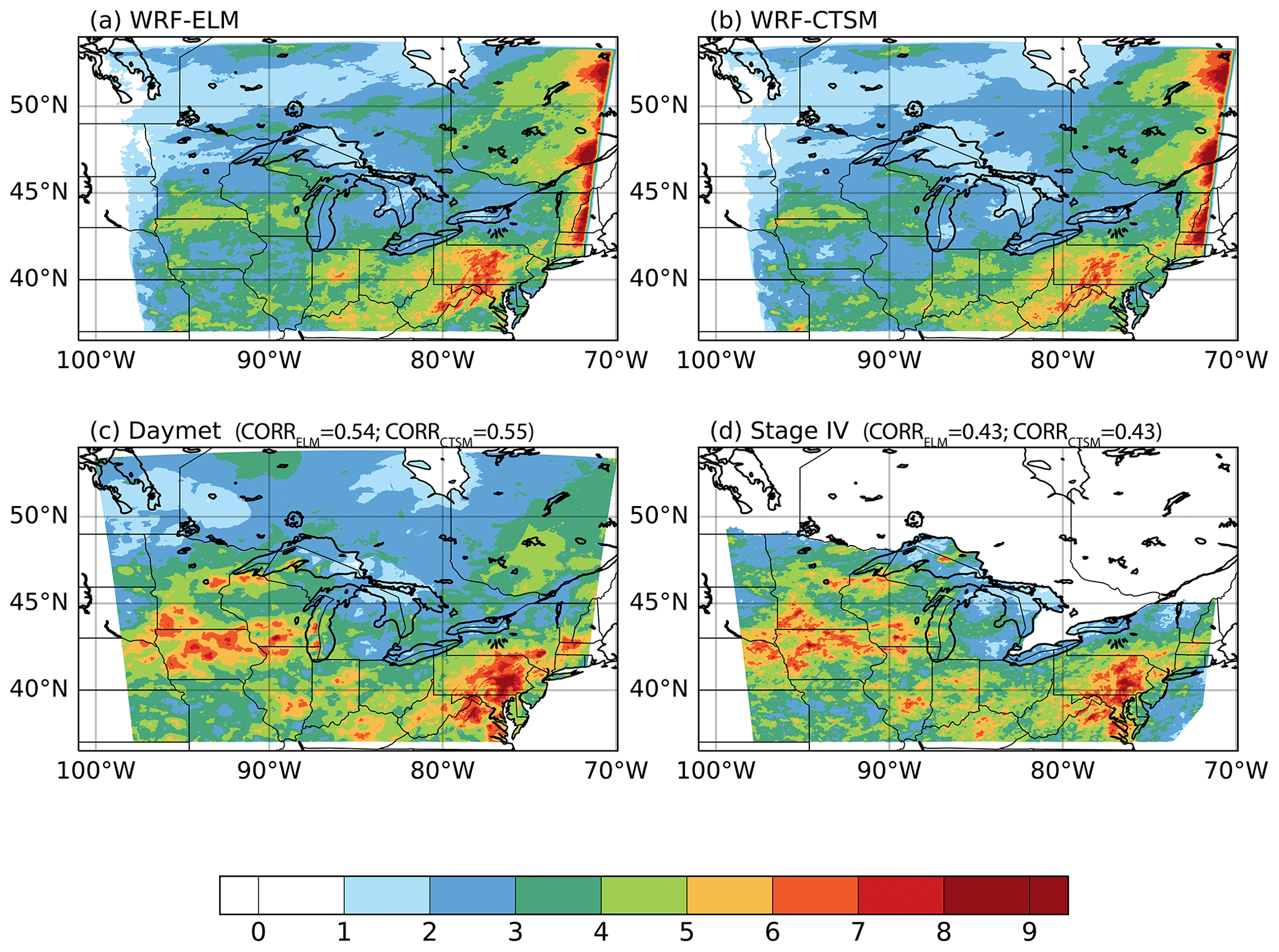
Figure 12 The spatial distribution of June–July–August precipitation (mm d⁻¹) in (a) WRF-ELM, (b) WRF-CTSM, (c) Daymet, and (d) stage IV. The numbers on the top right of (c)–(d) indicate the CORR between each observational product and the two simulation results.

3.3.3 Precipitation

Figure 12 presents the spatial distribution of precipitation from models and observations. It is important to note that stage IV primarily focuses on the CONUS region, while significant areas of our simulation domain in Canada remain uncovered. Compared with Daymet (PRE_Daymet=3.55 mm d⁻¹), both WRF-ELM and WRF-CTSM capture the regional mean value (PRE_WRF-ELM=3.14 mm d⁻¹ and PRE_WRF-CTSM=2.96 mm d⁻¹) and the spatial distribution of precipitation, exhibiting CORR ranging from 0.43 to 0.55. The precipitation over the southeastern part of our study domain is well captured, while that on the western side of Lake Michigan is slightly underestimated, with WRF-ELM demonstrating a lower bias than WRF-CTSM. This underestimation of precipitation aligns with the underestimation of latent heat and evapotranspiration, suggesting that suppressed evapotranspiration may reduce moisture availability and transport, particularly to the western GLR. Conversely, an overestimation of precipitation is evident along the eastern boundary of our study domain.

4 Discussion and conclusions

This study introduces a framework integrating the state-of-the-art land surface model, ELM, with the widely used regional weather and climate model, WRF, named WRF-ELM. Moving beyond the traditional way of coupling between LSMs and WRF through internal subroutines within the WRF codebase. We adopt the LILAC–ESMF framework, a modular approach which maintains the integrity of ELM's source code structure and facilitates the transfer of future developments in ELM to WRF-ELM. After coupling the two models, simulations using WRF-ELM have been conducted over the Great Lakes region, and their performance has been evaluated against observations and reanalysis data from multiple sources and the WRF-CTSM simulations. These model simulations have been conducted at a resolution of 4 km × 4 km, facilitating direct model validation and verification with various data sources. The use of seasonal mean simulation outputs and diurnal cycles showcases the capabilities of WRF-ELM in representing the temporal and spatial variations in water and energy cycles over the Great Lakes region.

In general, our findings suggest that the newly coupled WRF-ELM effectively captures the spatial distribution of surface state variables and fluxes across the GLR. The model displays a smoother gradient in surface skin temperature than WRF-CTSM due to the representation of subgrid features within grid cells. The model's performance is particularly reasonable over the natural vegetation, while a minor warm bias is detected over crop and urban grids.

The slight overestimation of air temperature in crop regions could potentially be mitigated by incorporating a more realistic representation of crops, such as crop rotation and irrigation. Additionally, the application of spatially varying crop parameters closely captures the observed magnitude and seasonality of carbon and energy fluxes compared to the observations (Sinha et al., 2023). However, these improvements have only been tested using the land-only ELM. Our generalized coupling framework supports future studies of sophisticated crop–atmosphere interactions at finer spatial resolution than those achieved with coarse GCM simulations.

In addition, the UHI effects in cities surrounding the GLR are generally captured in both WRF-ELM and WRF-CTSM, as indicated by the warmer night temperature in the cities. While there is an overestimation of UHI compared to ASOS, this could be due to the simplified urban representation in ELM. For instance, the urban surface emissivity in CLM, and thus ELM due to the shared model structure, is reported to be noticeably lower than the values derived from satellites, resulting in a surface UHI effect that is significantly higher than satellite-derived values (Chakraborty et al., 2021). Another potential contributing factor could be the lack of representation of urban vegetation. The presence of vegetation tends to mitigate the UHI effect (Paschalis et al., 2021), and its absence in the urban subgrid would lead to an overestimation of UHI values, with all else remaining equal.

Our research develops the WRF-ELM framework and provides the first assessment of its capabilities through high-resolution model simulations that fully capture expected patterns of land–atmosphere interactions. Based on the validation and assessment of WRF-ELM results, this study delivers a baseline reference, identifies common model biases in high-resolution regional applications, and proposes pathways for subsequent model development for ELM, as well as the coupled model. The coupled model provides an opportunity to investigate the impact of more sophisticated land processes, such as plant hydraulics, dynamic vegetation distributions, and soil biogeochemistry, on weather and climate predictions.