Graphics-processing-unit-accelerated ice flow solver for unstructured meshes using the Shallow-Shelf Approximation (FastIceFlo v1.0.1)

Ice-sheet flow models capable of accurately projecting their future mass balance constitute tools to improve flood risk assessment and assist sea-level rise mitigation associated with enhanced ice discharge. Some processes that need to be captured, such as grounding-line migration, require high spatial resolution (under the kilometer scale). Conventional ice flow models mainly execute on central processing units (CPUs), which feature limited parallel processing capabilities and peak memory bandwidth. This may hinder model scalability and result in long run times, requiring significant computational resources. As an alternative, graphics processing units (GPUs) are ideally suited for high spatial resolution, as the calculations can be performed concurrently by thousands of threads, processing most of the computational domain simultaneously. In this study, we combine a GPU-based approach with the pseudo-transient (PT) method, an accelerated iterative and matrix-free solution strategy, and investigate its performance for finite elements and unstructured meshes with application to two-dimensional (2-D) models of real glaciers at a regional scale. For both the Jakobshavn and Pine Island glacier models, the number of nonlinear PT iterations required to converge a given number of vertices (N) scales in the order of 𝒪(N^1.2) or better. We further compare the performance of the PT CUDA C implementation with a standard finite-element CPU-based implementation using the price-to-performance metric. The price of a single Tesla V100 GPU is 1.5 times that of two Intel Xeon Gold 6140 CPUs. We expect a minimum speedup of at least 1.5 times to justify the Tesla V100 GPU price to performance. Our developments result in a GPU-based implementation that achieves this goal with a speedup beyond 1.5 times. This study represents a first step toward leveraging GPU processing power, enabling more accurate polar ice discharge predictions. The insights gained will benefit efforts to diminish spatial resolution constraints at higher computing performance. The higher computing performance will allow for ensembles of ice-sheet flow simulations to be run at the continental scale and higher resolution, a previously challenging task. The advances will further enable the quantification of model sensitivity to changes in upcoming climate forcings. These findings will significantly benefit process-oriented sea-level-projection studies over the coming decades.

1 Introduction

Global mean sea level is rising at an average rate of 3.7 mm yr⁻¹, posing a significant threat to coastal communities and global ecosystems (Hinkel et al., 2014; Kopp et al., 2016). The increase in ice discharge from the Greenland and Antarctic ice sheets significantly contributes to sea-level rise. However, their dynamic response to climate change remains a fundamental uncertainty in future projection (Rietbroek et al., 2016; Chen et al., 2017; IPCC, 2021). While much progress has been made over the last decades, several critical physical processes, such as calving and ice-sheet basal sliding, remain poorly understood (Pattyn and Morlighem, 2020). Existing computational resources limit the spatial resolution and simulation time on which continental-scale ice-sheet models can run. Some processes, such as grounding-line migration or ice front dynamics, require spatial resolutions in the order of 1 km or smaller (Larour et al., 2012; Aschwanden et al., 2021; Castleman et al., 2022).

Most numerical models use a solution strategy designed to target central processing units (CPUs) and shared memory parallelization. CPUs' parallel processing capabilities, peak memory bandwidth, and power consumption remain limiting factors. It remains to be seen whether high-resolution modeling will become feasible at the continental scale (or ice-sheet scale). Specifically, complex flow models, such as full-Stokes models, may remain challenging to employ beyond the regional scale. Trying to overcome the technical limitations tied to CPU-based computing, graphics processing units (GPUs) feature interesting capabilities and have been booming over the past decade (Brædstrup et al., 2014; Häfner et al., 2021). Developing algorithms and solvers to leverage GPU computing capabilities has become essential and has resulted in active development within scientific computing and high-performance computing (HPC) communities.

The traditional way of solving the partial differential equations governing ice-sheet flow, employing, e.g., finite-element analysis, may represent a challenge to leverage GPU acceleration efficiently. Handling unstructured grid geometries and having global-to-local indexing patterns may significantly hinder efficient memory transfers and optimal bandwidth utilization. Räss et al. (2020) proposed an alternative approach by reformulating the flow equations in the form of pseudo-transient (PT) updates. The PT method augments the time-independent governing ice-sheet flow equation by physically motivated pseudo-time-dependent terms. The added pseudo-time τ terms turn the initial time-independent elliptic equations into a parabolic form, allowing for an explicit iterative pseudo-time integration to reach a steady state and, thus, the solution of the initial elliptic problem. The explicit pseudo-time integration scheme eliminates the need for the expensive direct–iterative type of solvers, making the proposed approach matrix-free and attractive for various parallel computing approaches (Frankel, 1950; Poliakov et al., 1993; Kelley and Liao, 2013). Räss et al. (2020) introduced this method specifically targeting GPU computing to enable the development of high-spatial-resolution full-Stokes ice-sheet flow solvers in two dimensions (2-D) and three dimensions (3-D), respectively, on uniform grids (Räss et al., 2020). The approach unveils a promising solution strategy, but the finite-difference discretization on uniform and structured grids and the idealized test cases represent actual limitations.

Here, we build upon work from previous studies (Räss et al., 2019, 2020) on the accelerated PT method for finite-difference discretization on uniform, structured grids and extend it to finite-element discretization and unstructured meshes. We developed a CUDA C implementation of the PT depth-integrated Shallow-Shelf Approximation (SSA) and applied it to regional-scale glaciers, Pine Island Glacier and Jakobshavn Isbræ, in West Antarctica and Greenland, respectively. We compare the PT CUDA C implementation with a more standard finite-element CPU-based implementation available within the Ice-sheet and Sea-level System Model (ISSM). Our comparison uses the same mesh, model equations, and boundary conditions. In Sect. 2, we present the mathematical reformulation of the 2-D SSA momentum balance equations to incorporate the additional pseudo-transient terms needed for the PT method. We provide the weak formulation and discuss the spatial discretization. Section 3 describes the numerical experiments conducted, chosen glacier model configurations, hardware implementation, and performance assessment metrics. In Sects. 4 and 5, we illustrate the method's performance and conclude on future research directions.

2 Methods

2.1 Mathematical formulation of the 2-D SSA model

We employ the SSA (MacAyeal, 1989) formulation to solve the momentum balance equation:

$$\begin{array}{}\text{(1)}& \mathrm{\nabla }\cdot \left(\mathrm{2}H\mathit{\mu }{\dot{\mathit{\epsilon }}}_{\mathrm{SSA}}\right)=\mathit{\rho }gH\mathrm{\nabla }\mathit{s}+{\mathit{\alpha }}^{\mathbf{2}}\mathit{v},\end{array}$$

where the 2-D SSA strain rate ${\dot{\mathit{\epsilon }}}_{\mathrm{SSA}}$ is defined as

$$\begin{array}{}\text{(2)}& {\dot{\mathit{\epsilon }}}_{\mathrm{SSA}}=\left(\begin{array}{cc}\mathrm{2}\frac{\partial v_x}{\partial x}+\frac{\partial v_y}{\partial y}& \frac{\partial v_x}{\partial y}\\ & \\ \frac{\partial v_x}{\partial y}& \mathrm{2}\frac{\partial v_y}{\partial y}+\frac{\partial v_x}{\partial x}\end{array}\right).\end{array}$$

The terms v_x and v_y represent the respective x and y ice velocity components, H is the ice thickness, ρ is the ice density, g is the gravitational acceleration, s is the glacier's upper surface z coordinate, and α²v is the basal friction term. The ice viscosity μ follows Glen's flow law (Glen, 1955):

$$\begin{array}{}\text{(3)}& \mathit{\mu }={\displaystyle \frac{B}{\mathrm{2}{\dot{\mathit{\epsilon }}}_{\mathrm{e}}^{(n-\mathrm{1})/n}}},\end{array}$$

where B is ice rigidity, ${\dot{\mathit{\epsilon }}}_{\mathrm{e}}$ is the effective strain rate, and n=3 is Glen's power-law exponent. We regularize the strain-rate-dependent viscosity formulation in the numerical implementation by capping it at 1×10⁵ to address the singularity arising in regions of the computational domain where the strain rate tends toward zero.

As boundary conditions, we apply water pressure at the ice front Γ_σ and nonhomogeneous Dirichlet boundary conditions Γ_u on the other boundaries (based on observed velocity).

2.2 Mathematical reformulation of the 2-D SSA model to incorporate the PT method

The solution to the SSA ice flow problem is commonly achieved by discretizing Eq. (1) using the finite-element or finite-difference method. The discretized problem can be solved using a direct, direct–iterative, or iterative approach. Robust matrix-based direct-type solvers exhibit significant scaling limitations restricting their applicability when considering high-resolution or 3-D configurations. Iterative solving approaches allow one to circumvent most scaling limitations. However, they may encounter convergence issues for suboptimally conditioned, stiff, or highly nonlinear problems, resulting in the non-tractable growth of the iteration count. Thus, one challenge is to prevent the iteration count from growing exponentially. We propose the accelerated pseudo-transient (PT) method as an alternative approach. The method augments the steady-state viscous flow (Eq. 1) by adding the usually ignored transient term, which can be further used to integrate the equations in pseudo-time τ, seeking an implicit solution once the steady state is reached, i.e., when τ→∞.

Building upon work from previous studies (Omlin et al., 2018; Duretz et al., 2019; Räss et al., 2019, 2020, 2022), we reformulate the 2-D SSA steady-state momentum balance equations into a transient diffusion-like formulation for flow velocities v_x,y by incorporating the usually omitted time derivative.

$$\begin{array}{}\text{(4)}& \mathrm{\nabla }\cdot \left(\mathrm{2}H\mathit{\mu }{\dot{\mathit{\epsilon }}}_{\mathrm{SSA}}\right)-\mathit{\rho }gH\mathrm{\nabla }s-{\mathit{\alpha }}^{\mathrm{2}}\mathit{v}=\mathit{\rho }H{\displaystyle \frac{\partial \mathit{v}}{\partial \mathit{\tau }}}\end{array}$$

The velocity–time derivatives represent physically motivated expressions that we can further use to iteratively reach a steady state, which provides the solution of the original time-independent equations. As we are only interested in the steady-state here, transient processes evolve in numerical time or pseudo-time τ:

$$\begin{array}{}\text{(5)}& \begin{array}{r}\mathit{\rho }H{\displaystyle \frac{\partial v_x}{\partial \mathit{\tau }}}=R_x,\\ \mathit{\rho }H{\displaystyle \frac{\partial v_y}{\partial \mathit{\tau }}}=R_y,\end{array}\end{array}$$

where R_x and R_y correspond to the right-hand-side expressions of Eq. (1) and define the residuals of the original SSA equations for which we are seeking a solution. We define the transient pseudo-time step Δτ as a field variable (that is spatially variable) chosen to minimize the number of nonlinear PT iterations.

2.3 Pseudo-time-stepping method

Here, we advance in numerical pseudo-time using a forward Euler pseudo-time-stepping method. We choose our time derivative by approximating the transient diffusive system for both v_x and v_y:

$$\begin{array}{}\text{(6)}& \begin{array}{rl}\mathit{\rho }H{\displaystyle \frac{\partial v_x}{\partial \mathit{\tau }}}& ={\displaystyle \frac{\partial }{\partial x}}\left(\mathrm{4}H\mathit{\mu }{\displaystyle \frac{\partial v_x}{\partial x}}\right),\\ \mathit{\rho }H{\displaystyle \frac{\partial v_y}{\partial \mathit{\tau }}}& ={\displaystyle \frac{\partial }{\partial y}}\left(\mathrm{4}H\mathit{\mu }{\displaystyle \frac{\partial v_y}{\partial y}}\right),\end{array}\end{array}$$

where one recognizes the diffusive variables v_x,y and the effective dynamic viscosity $\mathrm{4}\mathit{\mu }/\mathit{\rho }$ as a diffusion coefficient. Using the analogy of a diffusive process, we can define a CFL (Courant–Friedrichs–Lewy)-like stability criterion for the PT iterative scheme. The explicit CFL-stability-based time step for viscous flow is given by the following:

$$\begin{array}{}\text{(7)}& \mathrm{\Delta }{\mathit{\tau }}_{\max }=\mathit{\rho }{\displaystyle \frac{\mathrm{\Delta }{x}^{\mathrm{2}}}{\mathrm{4}\mathit{\mu }(\mathrm{1}+{\mathit{\mu }}_{\mathrm{b}})\times n_{\dim }}},\end{array}$$

where Δx represents the grid spacing, μ_b is the numerical bulk ice viscosity, and $n_{\dim }=\mathrm{2.1},\mathrm{4.1}$, and 6.1 in 1-D, 2-D, and 3-D, respectively.

2.4 Viscosity continuation

We implement a continuation on the nonlinear strain-rate-dependent effective viscosity μ_eff to avoid the iterative solution process diverging, as strain-rate values may not satisfy the momentum balance at the beginning of the iterative process and may, thus, be far from equilibrium. At every pseudo-time step, the effective viscosity μ_eff is updated in the logarithmic space:

$$\begin{array}{}\text{(8)}& {\mathit{\mu }}_{\mathrm{eff}}=\exp \left({\mathit{\theta }}_{\mathit{\mu }}\log \left(\mathit{\mu }\right)+(\mathrm{1}-{\mathit{\theta }}_{\mathit{\mu }})\log ({\mathit{\mu }}_{\mathrm{eff}}^{\mathrm{old}}\right),\end{array}$$

where the scalar ${\mathrm{10}}^{-\mathrm{2}}<{\mathit{\theta }}_{\mathit{\mu }}<\mathrm{1}$ is selected such that we provide sufficient time to relax the nonlinear viscosity at the start of the pseudo-iterative loop.

2.5 Acceleration owing to damping

The major limitation of this simple first-order, or Picard-type, iterative approach resides in the poor iteration count scaling with increased numerical resolution. The number of iterations needed to converge for a given problem for N number of grid points involved in the computation scales in the order of 𝒪(N²).

To address this limitation, we consider a second-order method, referred to as the second-order Richardson method, as introduced by Frankel (1950). This approach allows us to aggressively reduce the number of iterations to the number of grid points, making the method scale as ≈𝒪(N^1.2). Optimal scaling can be achieved by realizing that the PT framework's diffusion type of updates readily provided can be divided into two wave-like update steps. Transitioning from diffusion to wave-like pseudo-physics exhibits two main advantages: (i) the wave-like time step limit is a function of Δx instead of Δx²; (ii) it is possible to turn the wave equation into a damped wave equation. The latter permits one to find optimal tuning parameters to achieve optimal damping, resulting in fast convergence. Let us assume the following diffusion-like update step, reported here for the x direction only:

$$\begin{array}{}\text{(9)}& {\displaystyle }\mathit{\rho }H{\displaystyle \frac{\partial v_x}{\partial \mathit{\tau }}}={\displaystyle \frac{\partial }{\partial x}}\mathrm{4}H\mathit{\mu }{\displaystyle \frac{\partial v_x}{\partial x}}.\end{array}$$

The above expression results in the following update rule:

$$\begin{array}{}\text{(10)}& {\displaystyle }{v}_x=v_x^{\mathrm{old}}+{\displaystyle \frac{\mathrm{\Delta }{\mathit{\tau }}_{\mathrm{D}}}{\mathit{\rho }H}}\left({\displaystyle \frac{\partial }{\partial x}}\mathrm{4}H\mathit{\mu }{\displaystyle \frac{\partial v_x}{\partial x}}\right),\end{array}$$

where $\mathrm{\Delta }{\mathit{\tau }}_{\mathrm{D}}\approx \mathrm{\Delta }{x}^{\mathrm{2}}/(\mathrm{4}\mathit{\mu }/\mathit{\rho })/\mathrm{4.1}$ is the diffusion-like time step limit. This system can be separated into a residual assignment A_x and the velocity update v_x:

$$\begin{array}{}\text{(11)}& {\displaystyle }{A}_x& {\displaystyle }={\displaystyle \frac{\mathrm{1}}{\mathit{\rho }H}}\left({\displaystyle \frac{\partial }{\partial x}}\mathrm{4}H\mathit{\mu }{\displaystyle \frac{\partial v_x}{\partial x}}\right),\text{(12)}& {\displaystyle }{v}_x& {\displaystyle }=v_x^{\mathrm{old}}+\mathrm{\Delta }{\mathit{\tau }}_{\mathrm{D}}{A}_x.\end{array}$$

Converting Eq. (11) into an update rule using a step size of (1−γ),

$$\begin{array}{}\text{(13)}& {\displaystyle }{A}_x{\displaystyle }=A_x^{\mathrm{old}}(\mathrm{1}-\mathit{\gamma })+{\displaystyle \frac{\mathrm{1}}{\mathit{\rho }H}}\left({\displaystyle \frac{\partial }{\partial x}}\mathrm{4}H\mathit{\mu }{\displaystyle \frac{\partial v_x}{\partial x}}\right),\end{array}$$

turns the system composed of Eqs. (12) and (13) into a damped wave equation similar to what was suggested by Frankel (1950). Ideal convergence can be reached upon selecting the appropriate damping parameter γ. To maintain solution stability, we include relaxation θ_v:

$$\begin{array}{}\text{(14)}& {\displaystyle }{v}_x{\displaystyle }=v_x^{\mathrm{old}}+{\mathit{\theta }}_v\mathrm{\Delta }{\mathit{\tau }}_{\mathrm{D}}{A}_x,\end{array}$$

where $\mathrm{0}<\mathit{\gamma }<\mathrm{1}$ and $\mathrm{0}<{\mathit{\theta }}_v<\mathrm{1}$.

Alternative and complementary details about the PT acceleration can be found in Räss et al. (2019), Duretz et al. (2019), and Räss et al. (2020), while an in-depth analysis is provided in Räss et al. (2022).

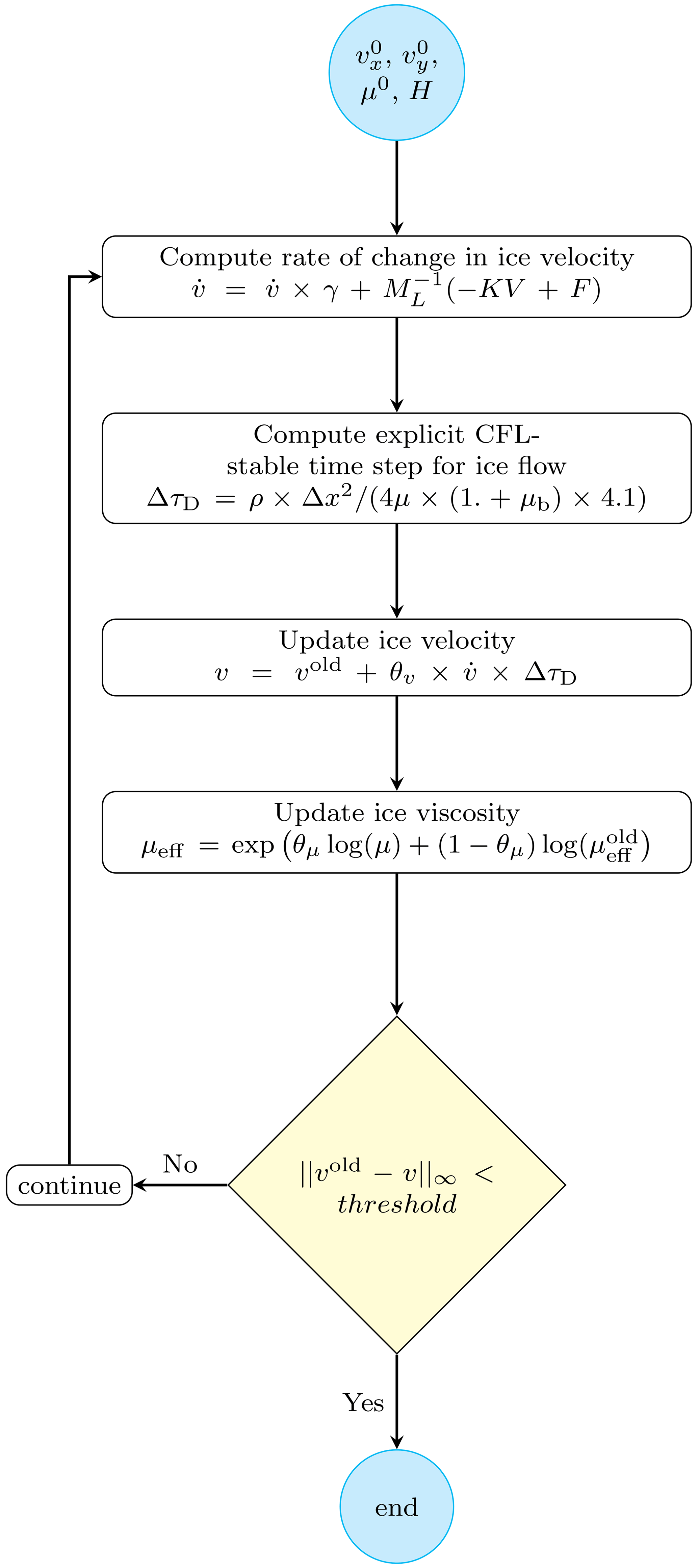
Figure 1 PT iterative algorithm for unstructured meshes applied to solve 2-D SSA momentum balance equations.

2.6 Weak formulation and finite-element discretization

Using the PT method, the equations to solve are as referenced in Eq. (4):

$$\begin{array}{}\text{(15)}& \mathit{\rho }H{\displaystyle \frac{\partial \mathit{v}}{\partial \mathit{\tau }}}=\mathrm{\nabla }\cdot \mathrm{2}H\mathit{\mu }{\dot{\mathit{\epsilon }}}_{\mathrm{SSA}}-\mathit{\rho }gH\mathrm{\nabla }s-{\mathit{\alpha }}^{\mathrm{2}}\mathit{v}.\end{array}$$

The weak form of the equation, assuming homogeneous Dirichlet conditions along all model boundaries for simplicity, reads: $\forall \mathit{w}\in {\mathcal{H}}^{\mathrm{1}}\left(\mathrm{\Omega }\right)$,

$$\begin{array}{}\text{(16)}& \begin{array}{rl}\underset{\mathrm{\Omega }}{\int }\mathit{\rho }H{\displaystyle \frac{\partial \mathit{v}}{\partial \mathit{\tau }}}\cdot \mathbf{w}\mathrm{d}\mathrm{\Omega }& +\underset{\mathrm{\Omega }}{\int }\mathrm{2}H\mathit{\mu }{\dot{\mathit{\epsilon }}}_{\mathrm{SSA}}\cdot \mathrm{\nabla }\mathit{w}\mathrm{d}\mathrm{\Omega }=\\ & \underset{\mathrm{\Omega }}{\int }-\mathit{\rho }gH\mathrm{\nabla }s\cdot \mathit{w}-{\mathit{\alpha }}^{\mathrm{2}}\mathit{v}\cdot \mathit{w}\mathrm{d}\mathrm{\Omega },\end{array}\end{array}$$

where ℋ¹(Ω) is the space of square-integrable functions whose first derivatives are also square integrable.

Once discretized using the finite-element method, the matrix system to solve reads:

$$\begin{array}{}\text{(17)}& \mathbf{M}\dot{\mathit{V}}+\mathbf{K}\mathit{V}=\mathit{F},\end{array}$$

where M is the mass matrix, K is the stiffness matrix, F is the right-hand-side or load vector, and V is the vector of ice velocity.

We can compute $\dot{\mathbf{V}}$ by solving

$$\begin{array}{}\text{(18)}& \dot{\mathbf{V}}\simeq {\mathbf{M}}_{\mathrm{L}}^{-\mathrm{1}}\left(-\mathbf{KV}+\mathit{F}\right),\end{array}$$

where M_L stands for the lumped mass matrix that permits one to avoid the resolution of a matrix system.

Hence, we have an explicit expression of the time derivative of the ice velocity for each vertex of the mesh:

$$\begin{array}{}\text{(19)}& {\displaystyle }\begin{array}{rl}{\dot{v}}_{xi}=& {\displaystyle \frac{\mathrm{1}}{\mathit{\rho }H{m}_{\mathrm{L}i}}}\left(-\underset{\mathrm{\Omega }}{\int }\left(\mathrm{4}H\mathit{\mu }{\displaystyle \frac{\partial v_x}{\partial x}}+\mathrm{2}H\mathit{\mu }{\displaystyle \frac{\partial v_y}{\partial y}}\right){\displaystyle \frac{\partial {\mathit{\phi }}_i}{\partial x}}\right.\\ & +\left(H\mathit{\mu }{\displaystyle \frac{\partial v_x}{\partial y}}+H\mathit{\mu }{\displaystyle \frac{\partial v_y}{\partial x}}\right){\displaystyle \frac{\partial {\mathit{\phi }}_i}{\partial y}}\mathrm{d}\mathrm{\Omega }\\ & +\left.\underset{\mathrm{\Omega }}{\int }-\mathit{\rho }gH{\displaystyle \frac{\partial s}{\partial x}}{\mathit{\phi }}_i-{\mathit{\alpha }}^{\mathrm{2}}{v}_x{\mathit{\phi }}_i\mathrm{d}\mathrm{\Omega }\right),\end{array}\text{(20)}& {\displaystyle }\begin{array}{rl}{\dot{v}}_{yi}=& {\displaystyle \frac{\mathrm{1}}{\mathit{\rho }H{m}_{\mathrm{L}i}}}\left(-\underset{\mathrm{\Omega }}{\int }\left(\mathrm{4}H\mathit{\mu }{\displaystyle \frac{\partial v_y}{\partial y}}+\mathrm{2}H\mathit{\mu }{\displaystyle \frac{\partial v_x}{\partial x}}\right){\displaystyle \frac{\partial {\mathit{\phi }}_i}{\partial y}}\right.\\ & +\left(H\mathit{\mu }{\displaystyle \frac{\partial v_x}{\partial y}}+H\mathit{\mu }{\displaystyle \frac{\partial v_y}{\partial x}}\right){\displaystyle \frac{\partial {\mathit{\phi }}_i}{\partial x}}\mathrm{d}\mathrm{\Omega }\\ & \left.+\underset{\mathrm{\Omega }}{\int }-\mathit{\rho }gH{\displaystyle \frac{\partial s}{\partial y}}{\mathit{\phi }}_i-{\mathit{\alpha }}^{\mathrm{2}}{v}_y{\mathit{\phi }}_i\mathrm{d}\mathrm{\Omega }\right),\end{array}\end{array}$$

where m_Li is the component number i along the diagonal of the lumped mass matrix M_L.

For every nonlinear PT iteration, we compute the rate of change in velocity $\dot{\mathit{v}}$ and the explicit CFL-stability-based time step Δτ. We then deploy the reformulated 2-D SSA momentum balance equations to update ice velocity v followed by ice viscosity μ_eff. We iterate in pseudo-time until the stopping criterion is met (Fig. 1).

3 Numerical experiments

3.1 Glacier model configurations

To test the performance of the PT method beyond simple idealized geometries, we apply it to two regional-scale glaciers: Jakobshavn Isbræ, in Western Greenland, and Pine Island Glacier, in West Antarctica (Fig. 2). For Jakobshavn Isbræ, we rely on BedMachine Greenland v4 (Morlighem et al., 2017) and also invert for basal friction to infer the basal boundary conditions. Note that the inversion is run on the Ice-sheet and Sea-level System Model (ISSM), using a standard approach (Larour et al., 2012). For Pine Island Glacier, we initialize the ice geometry using BedMachine Antarctica v2 (Morlighem et al., 2020) and infer the friction coefficient using surface velocities derived from satellite interferometry (Rignot et al., 2011).

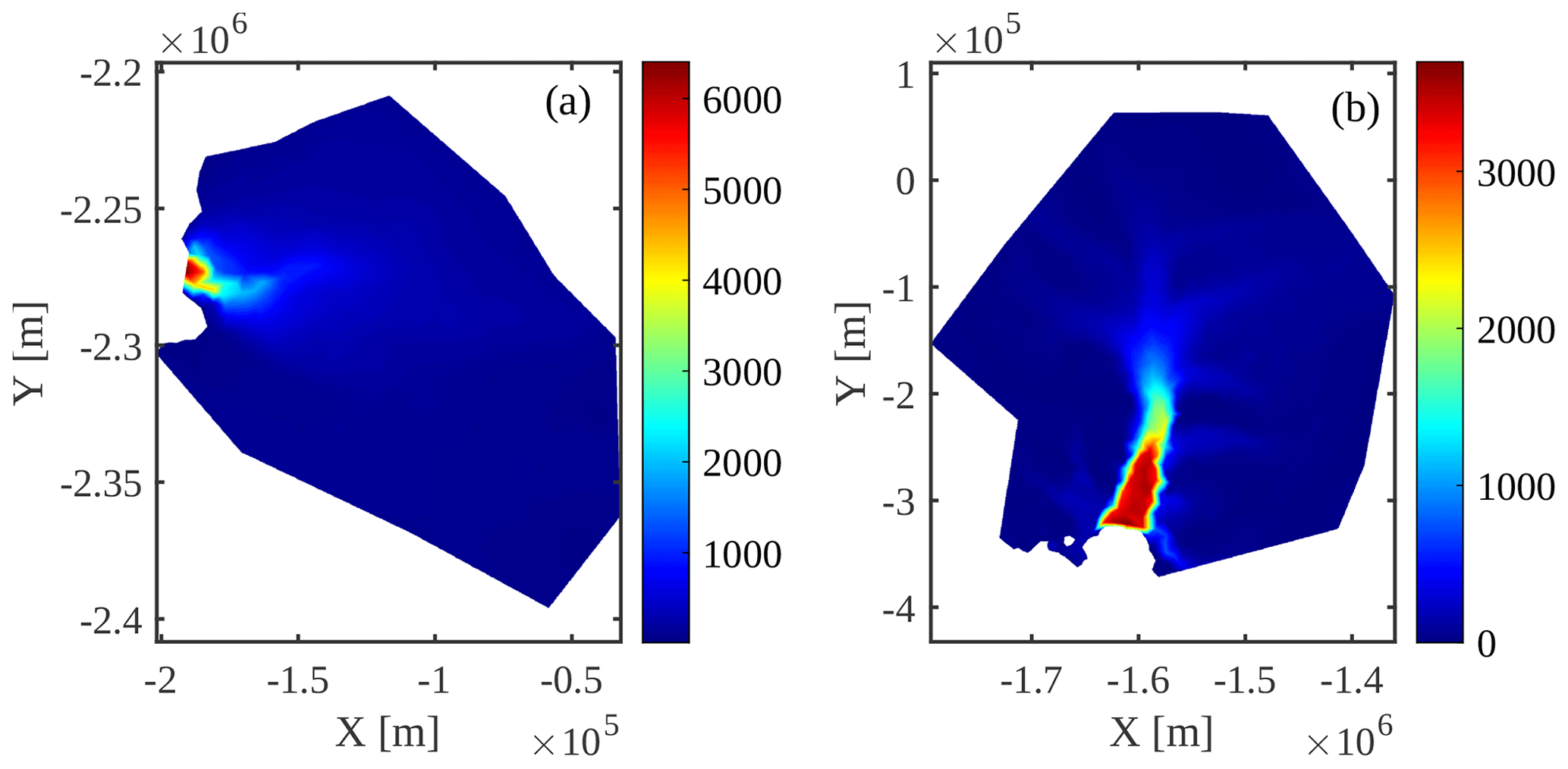
Figure 2 Glacier model configurations: observed surface velocities (in m yr⁻¹) interpolated on a uniform mesh. Panels (a) and (b) correspond to Jakobshavn Isbræ and Pine Island Glacier, respectively.

3.2 Hardware implementation

We developed a CUDA C implementation to solve the SSA equations using the PT approach on unstructured meshes. We choose a stopping criterion of $\left|\right|v^{\mathrm{old}}-v|{|}_{\mathrm{\infty }}<\mathrm{10}$ m yr⁻¹. The software solves the 2-D SSA momentum balance equations on a single GPU. We use an NVIDIA Tesla V100 SXM2 GPU with 16 GB (gigabytes) of device RAM and an NVIDIA A100 SXM4 with 80 GB of device RAM. We compare the PT implementation's results on a Tesla V100 GPU with ISSM's “standard” CPU implementation using a conjugate gradient (CG) iterative solver. We used a 64-bit 18-core Intel Xeon Gold 6140 processor for the CPU comparison, with 192 GB of RAM available. We perform multicore Message Passing Interface (MPI)-parallelized ice-sheet flow simulations on two CPUs, with all 36 cores enabled (Larour et al., 2012; Habbal et al., 2017). All simulations use double-precision arithmetic computations.

3.3 Performance assessment metrics

To investigate the PT CUDA C implementation for unstructured meshes, we report the number of vertices (or grid size) and the corresponding number of nonlinear PT iterations needed to meet the stopping criterion. We employ the computational time required to reach convergence as a proxy to assess and compare the performance of the PT CUDA C with the ISSM CG CPU implementation. We make sure to exclude all pre- and post-processing steps from the timing. We quantify the relative performance of the CPU and GPU implementations as the speedup (S), given by the following:

$$\begin{array}{}\text{(21)}& S={\displaystyle \frac{t_{\mathrm{CPU}}}{t_{\mathrm{GPU}}}}.\end{array}$$

The PT method employed to solve the nonlinear momentum balance equations results in a memory-bound algorithm (Räss et al., 2020); therefore, the wall time depends on the memory throughput. In addition to the speedup, we employ the effective memory throughput metric to assess the performance of the PT CUDA C implementation developed in this study (Räss et al., 2020, 2022), which is defined as follows:

$$\begin{array}{}\text{(22)}& {\displaystyle }{T}_{\mathrm{eff}}={\displaystyle \frac{n_{\mathrm{n}}{n}_{\mathrm{iter}}{n}_{\mathrm{IO}}{n}_{\mathrm{p}}}{{\mathrm{1024}}^{\mathrm{3}}{t}_{n_{\mathrm{iter}}}}},\end{array}$$

where n_n represents the total number of vertices, n_iter is a given number of PT iterations, n_p is the arithmetic precision, $t_{n_{\mathrm{iter}}}$ is the time taken to complete n_iter iterations, and n_IO is the minimal number of nonredundant memory accesses (read and write operations). The number of read and write operations needed for this study would be eight: update v_x, v_y, and nonlinear viscosity arrays for every PT iteration, in addition to reading the basal friction coefficient and the masks.

4 Results and discussion

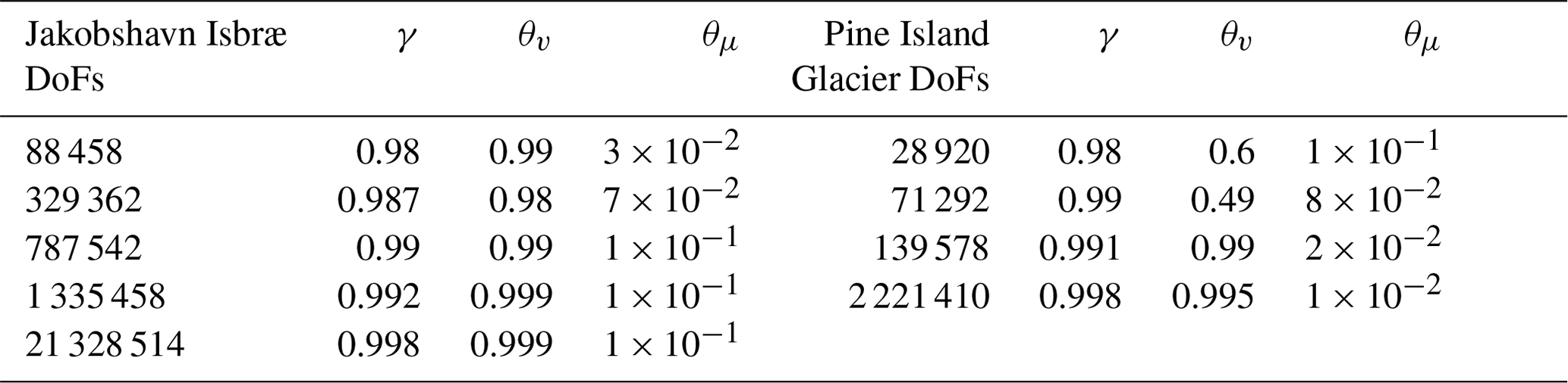
To investigate the performance of the PT CUDA C implementation on unstructured meshes, we report the number of vertices (or grid size) and the corresponding number of nonlinear PT iterations needed to meet the stopping criterion (Fig. 3). For both the Jakobshavn and Pine Island glacier models, the number of nonlinear PT iterations required to converge for a given number of vertices (N) scales in the order of ≈𝒪(N^1.2) or better. We chose the damping parameter γ, nonlinear viscosity relaxation scalar θ_μ, and transient pseudo-time step Δτ to maintain the linear scaling described above; optimal parameter values are listed in the Appendix (Table A1). We observed an exception at $\sim \mathrm{3}\times {\mathrm{10}}^{\mathrm{7}}$ degrees of freedom (DoFs) for the Pine Island Glacier model; optimal parameter values are unidentifiable. We will further investigate the convergence for the Pine Island Glacier model at $\sim \mathrm{3}\times {\mathrm{10}}^{\mathrm{7}}$ DoFs. Among the two glacier models chosen in this study, for a given number of vertices (N), Jakobshavn Isbræ resulted in faster convergence rates, which we attribute to differences in scale and bed topography and the nonlinearity of the problem (Fig. 4).

Figure 3 Performance assessment of the PT CUDA C implementation for unstructured meshes.

Figure 4 Residual error evolution of the PT CUDA C implementation for unstructured meshes.

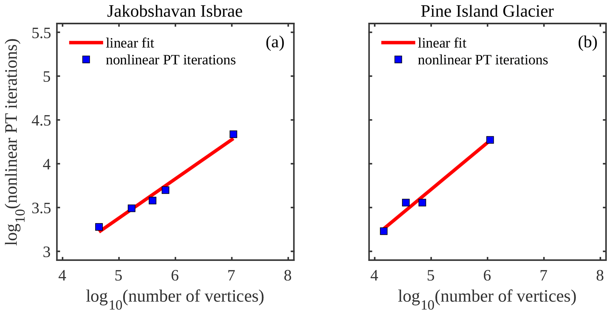
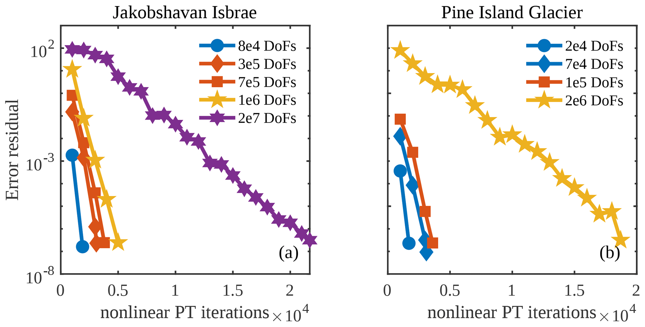
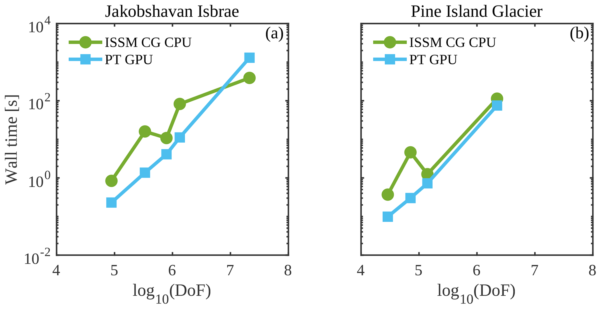
Figure 5 Performance comparison of the PT Tesla V100 implementation with the CPU implementation employing wall time (or computational time to reach convergence). Note that wall time does not include pre- and post-processing steps.

Table 1 Performance comparison of the PT Tesla V100 implementation with the CPU implementation employing speedup S.

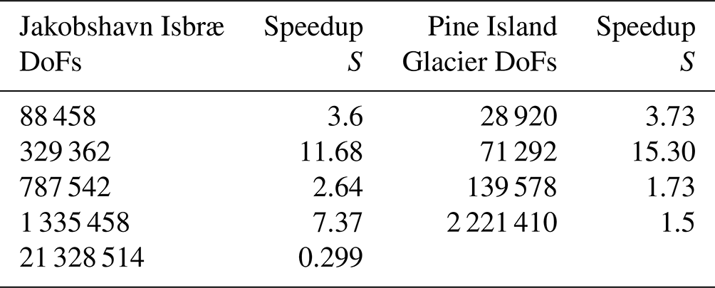
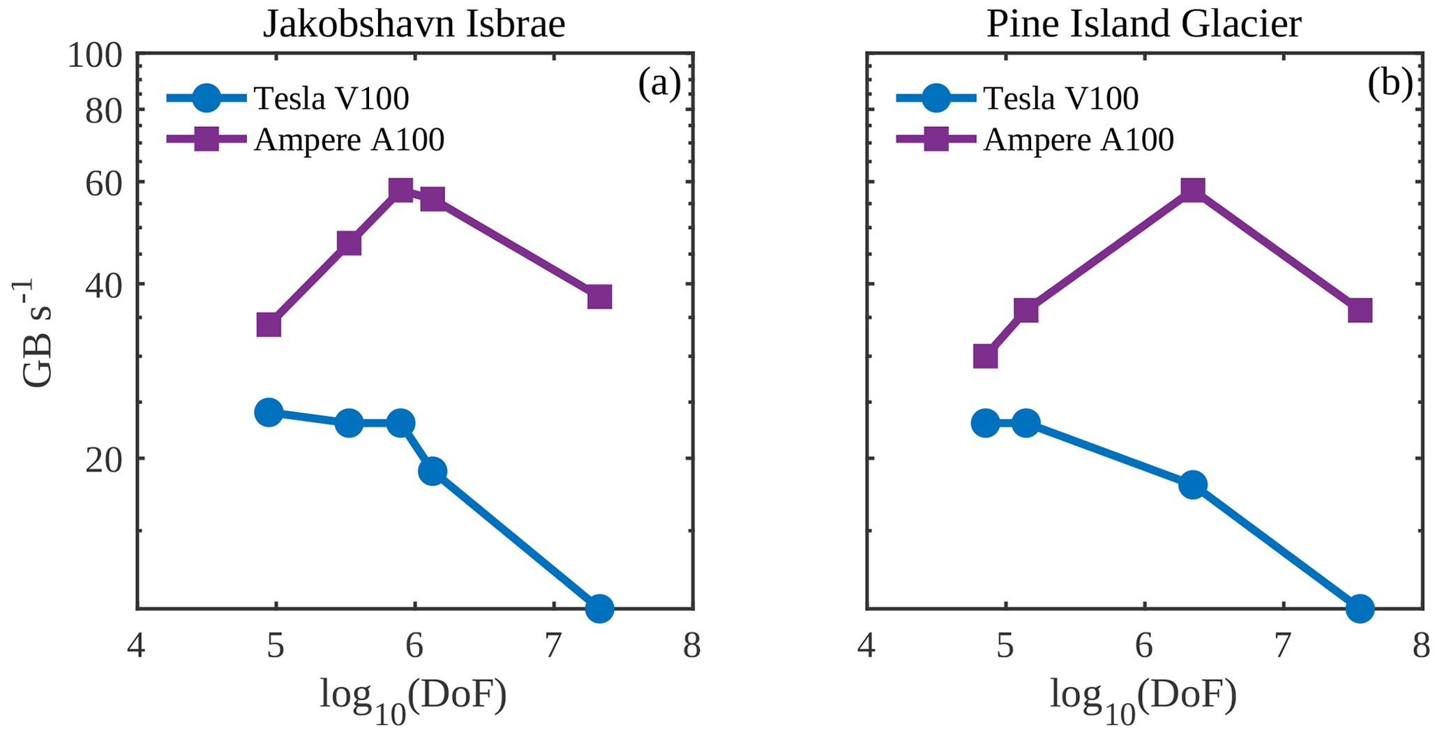
Figure 6 Performance assessment of the PT CUDA C implementation across GPU architectures employing effective memory throughput.

We further compare the performance of the PT CUDA C implementation with a standard finite-element CPU-based implementation using the price-to-performance metric. The price of a single Tesla V100 GPU is 1.5 times that of two Intel Xeon Gold 6140 CPU processors. ¹ We expect a minimum speedup of at least 1.5 times to justify the Tesla V100 GPU price to performance. We recorded the computational time to reach convergence for the ISSM CG CPU and the PT GPU solver implementations (Fig. 5) for up to 2×10⁷ DoFs. Across glacier configurations, we report a speedup of >1.5 times on the Tesla V100 GPU. We report a speedup of approximately 7 times at $\sim \mathrm{1}\times {\mathrm{10}}^{\mathrm{6}}$ DoFs for the Jakobshavn glacier model. This larger speedup at $\sim \mathrm{1}\times {\mathrm{10}}^{\mathrm{6}}$ DoFs indicates the PT GPU implementation's suitability to develop high-spatial-resolution ice-sheet flow models. We report an exception for the Jakobshavn glacier model at 2×10⁷ DoFs (speedup of 0.28 times). We suggest that readers compare the speedup results reported in this study (Table 1) with other parallelization strategies.

The PT method applied to solve nonlinear momentum balance equations is a memory-bound algorithm, as described in Sect. 3.3. The profiling results on the Tesla V100 GPU indicate an up to 85 % increase in the device's available memory resources utilization with the increase in DoFs. This further confirms the memory-bounded nature of the implementation. To assess the performance of the memory-bound PT CUDA C implementation, we employ the effective memory throughput metric defined in Sect. 3.3. We report the effective memory throughput to DoFs for the PT CUDA C single-GPU implementation (Fig. 6). We observe a significant drop in effective memory throughput on both GPU architectures at DoFs $>\times {\mathrm{10}}^{\mathrm{7}}$, which explains the drop in the speedup. We attribute the drop partly to the nonoptimal global memory access patterns reported in the L1TEX and L2 cache. We identify excessive nonlocal data access patterns in the ice stiffness and strain-rate computations, which involve accessing element-to-vertex connectivities and vice versa. For optimal or fully coalesced global memory access patterns, the threads in a warp must access the same relative address. We are investigating techniques to reduce the mesh non-localities and allow for coalesced global accesses.

We report a peak memory throughput for the NVIDIA Tesla V100 and A100 GPUs of 785 and 1536 GB s⁻¹, respectively. The peak memory throughput reflects the maximal memory transfer rates for performing memory copy-only operations. It represents the hardware performance limit in a memory-bound regime. Across glacier model configurations for the DoFs chosen in this study, the PT CUDA C implementation achieves a maximum of 23 and 58 GB s⁻¹ for the NVIDIA Tesla V100 and A100 GPUs, respectively. The measured memory throughput is in the order of 500 GB s⁻¹, as reported by the NVIDIA Nsight Compute profiling tool 2022.2 on the NVIDIA Tesla V100. The measured memory throughput values reflect that we efficiently saturate the memory bandwidth. In contrast, the lower effective memory throughput values indicate that some of the memory accesses are redundant and could be further optimized.

Minimizing the memory footprint is critical when assessing the performance of memory-bounded algorithms, further speedups, and increased ability to solve large-scale problems. Due to insufficient memory at 1×10⁸ DoFs for the Pine Island Glacier model configuration, we could neither execute the standard CPU solver on four 18-core Intel Xeon Gold 6140 processors and 3 TB of RAM nor the PT GPU implementation on the Tesla V100 GPU architecture. However, we could implement PT GPU on a single A100 SXM4 featuring 80 GB of device RAM. Thus, we could further confirm the necessity to keep the memory footprint minimal for models targeting high spatial resolution.

In this study, we tested up to an estimated 2×10⁷ DoFs needed to maintain a spatial resolution of ∼ 1 km or better in grounding-line regions for Antarctic and Greenland-wide ice flow models. Future studies may involve extending the PT CUDA C implementation from (i) the regional scale to the ice-sheet scale and from (ii) a 2-D SSA to a 3-D Blatter–Pattyn higher-order (HO) approximation. Extending the PT CUDA C implementation to the ice-sheet scale will require the user to carefully choose the damping parameter γ, nonlinear viscosity relaxation scalar θ_μ, and transient pseudo-time step Δτ. The shared elliptical nature of the 2-D SSA and 3-D HO formulations and corresponding partial differential-equation-based models (Gilbarg and Trudinger, 1977; Tezaur et al., 2015) suggests the PT method's ability to solve the 3-D HO momentum balance applied to unstructured meshes. The overarching goal is to diminish spatial resolution constraints at higher computing performance to improve predictions of ice-sheet evolution.

5 Conclusions

Recent studies have implemented techniques that keep computational resources manageable at the ice-sheet scale while increasing the spatial resolution dynamically in areas where the grounding lines migrate during prognostic simulations (Cornford et al., 2013; Goelzer et al., 2017). In terms of computer memory footprint and execution time, the computational cost associated with solving the momentum balance equations to predict the ice velocity and pressure represents one of the primary bottlenecks (Jouvet et al., 2022). This preliminary study introduces a PT solver, applied to unstructured meshes, that leverages the GPU computing power to alleviate this bottleneck. Coupling the GPU-based ice velocity and pressure simulations with CPU-based ice thickness and temperature simulations can provide an enhanced balance between speed and predictive performance.

This study aimed to investigate the PT CUDA C implementation for unstructured meshes and its application to the 2-D SSA model formulation. For both the Jakobshavn and Pine Island glacier models, the number of nonlinear PT iterations required to converge for a given number of vertices (N) scales in the order of ≈𝒪(N^1.2) or better. We observed an exception at 3×10⁷ degrees of freedom (DoFs) for the Pine Island Glacier model; optimal solver parameters are unidentifiable. We further compare the performance of the PT CUDA C implementation with a standard finite-element CPU-based implementation using the price-to-performance metric. We justify the GPU implementation in the price-to-performance metric for up to million-grid-point spatial resolutions.

In addition to the price-to-performance metric, we preliminary investigated the power consumption. The power consumption of the PT GPU implementation was measured using the NVIDIA System Management Interface 460.32.03. For the range of DoFs tested, the power usage for both glacier configurations to meet the stopping criterion was 38±1 W. The power consumption measurement for the CPU implementation was taken from the hardware specification sheet: thermal design power. For a 64-bit 18-core Intel Xeon Gold 6140 processor, the thermal design power is 140 W.² We executed the CPU-based multicore MPI-parallelized ice-sheet flow simulations on two CPUs, with all 36 cores enabled, and we chose the power consumption to be 280 W. This is a first-order estimate. Thus, the power consumption of the PT GPU implementation was approximately one-seventh of the traditional CPU implementation for the test cases chosen in this study. We will investigate this further.

This study represents a first step toward leveraging GPU processing power, enabling more accurate polar ice discharge predictions. The insights gained will benefit efforts to diminish spatial resolution constraints at higher computing performance. The higher computing performance will allow users to run ensembles of ice-sheet flow simulations at the continental scale and higher resolution, a previously challenging task. The advances will further enable the quantification of model sensitivity to changes in upcoming climate forcings. These findings will significantly benefit process-oriented sea-level-projection studies over the coming decades.

Appendix A

Table A1 Optimal combination of damping parameter γ, nonlinear viscosity relaxation scalar θ_μ, and relaxation θ_v to maintain the linear scaling and solution stability for the glacier model configurations and DoFs listed.