FastIsostasy v1.0 – a regional, accelerated 2D glacial isostatic adjustment (GIA) model accounting for the lateral variability of the solid Earth

The vast majority of ice-sheet modelling studies rely on simplified representations of the glacial isostatic adjustment (GIA), which, among other limitations, do not account for lateral variations in the lithospheric thickness and upper-mantle viscosity. In studies of the last glacial cycle using 3D GIA models, this has however been shown to have major impacts on the dynamics of marine-based sectors of Antarctica, which are likely to be the greatest contributors to sea-level rise in the coming centuries. This gap in comprehensiveness is explained by the fact that 3D GIA models are computationally expensive, rarely open-source and require a complex coupling scheme. To close this gap between “best” and “tractable” GIA models, we propose FastIsostasy here, a regional GIA model capturing lateral variations in the lithospheric thickness and mantle viscosity. By means of fast Fourier transforms and a hybrid collocation scheme to solve its underlying partial differential equation, FastIsostasy can simulate 100 000 years of high-resolution bedrock displacement in only minutes of single-CPU computation, including the changes in sea-surface height due to mass redistribution. Despite its 2D grid, FastIsostasy parameterises the depth-dependent viscosity and therefore represents the depth dimension to a certain extent. FastIsostasy is benchmarked here against analytical, as well as 1D and 3D numerical solutions, and shows good agreement with them. For a simulation of the last glacial cycle, its mean and maximal error over time and space respectively yield less than 5 % and 16 % compared to a 3D GIA model over the regional solution domain. FastIsostasy is open-source, is documented with many examples and provides a straightforward interface for coupling to an ice-sheet model. The model is benchmarked here based on its implementation in Julia, while a Fortran version is also provided to allow for compatibility with most existing ice-sheet models. The Julia version provides additional features, including a vast library of adaptive time-stepping methods and GPU support.

1 Introduction

1.1 GIA is an important feedback on ice-sheet dynamics

Glacial isostatic adjustment (GIA) denotes the crustal displacement that results from changes in the ice, liquid-water and sediment columns, as well as the associated changes in Earth's gravity and rotation axis (Mitrovica et al., 2001), ultimately altering the sea level (Farrell and Clark, 1976). In the present work, we focus on the deformation and gravitational effects. For ice sheets, the former is a net negative feedback on mass balance through the lapse rate of the troposphere, and both imply additional negative feedbacks on the dynamics of marine-based regions, where enhanced melting leads not only to a grounding-line retreat but also to a regional bedrock uplift and a decrease in the sea-surface height (SSH), due to the reduced load applied upon the solid Earth and the lesser gravitational pull of the ice sheet on the oceans (Gomez et al., 2010, 2012, 2015, 2018; Whitehouse et al., 2019). As depicted in Fig. 1, these effects combine in a decrease in relative sea level (RSL), which is defined as the difference between the SSH and the bedrock elevation. Compared to the retreated state (Fig. 1b), this decrease ultimately leads to a readvance of the grounding line (Fig. 1c and d), therefore conditioning the marine ice-sheet instability along with the buttressing effect from ice shelves (Gudmundsson et al., 2012). It was shown that the representation of the deformation and gravitational feedbacks can stabilise grounding lines on retrograde slopes (Gomez et al., 2010, 2012) and that a rapid bedrock uplift can prevent the collapse of marine-terminating glaciers that are transiently forced (Konrad et al., 2015, 2016). Furthermore, an uplifting bedrock might lead isolated bathymetric peaks to connect with the ice sheet, creating so-called pinning points (Adhikari et al., 2014) that further contribute to the stability of a marine ice sheet. Although the negative feedbacks are illustrated here for ice-sheet retreat, they conversely apply to ice-sheet growth.

In addition to these effects, recent work has shown that the ice-sheet evolution might be significantly affected by the forebulge dynamic on longer timescales, for which viscous effects become important. This process denotes the region of comparatively small bedrock uplift (subsidence) surrounding a region of pronounced bedrock subsidence (uplift), which results from a positive (negative) surface load anomaly. Albrecht et al. (2023) suggest that the forebulge formation represents a positive feedback on ice-sheet growth through a decrease in the RSL close to the ice-sheet margin, and Kreuzer et al. (2023) show that a subsiding forebulge can increase sub-shelf melting through the formation of oceanic gateways that ease the intrusion of warm circumpolar deep water.

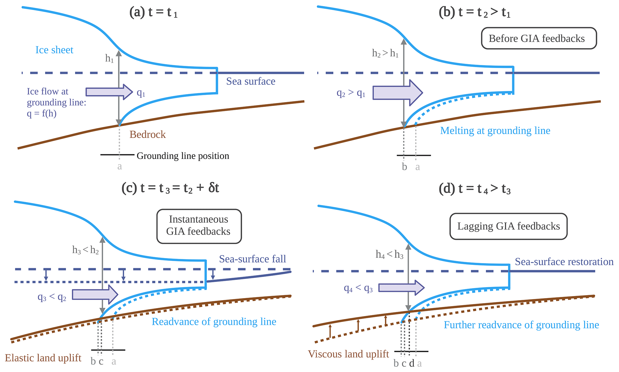
Figure 1 Idealised representation, adapted from Whitehouse et al. (2019), of the negative GIA feedbacks on marine-terminating glaciers with retrograde bedrock (e.g. Gomez et al., 2010). We perturb (a) the initial configuration of the ice sheet by (b) enhanced sub-shelf melting, leading to grounding-line retreat and therefore larger thickness and increased outflow at the grounding line. (c) The loss of ice leads to an instantaneous (δt≪1 year) decrease in the RSL, which can be decomposed into an elastic uplift of the bedrock and a decrease in the SSH due to the reduction in the gravitational pull on the ocean, leading to a readvance of the grounding line. (d) The elastic uplift is followed by a larger, viscous uplift which further readvances the grounding line and compensates the mass anomaly generated by the ice loss, therefore restoring the SSH close to its original value. The dashed lines used for the ice and the bedrock contour represent their original position (a).

1.2 Laterally variable structure of the solid Earth modulates GIA

For a given load applied to the solid Earth, the timescale of bedrock deformation is determined by the horizontal extent of the load and the mantle viscosity. The amplitude and the pattern of deformation are in turn determined by the magnitude of the load, the mantle density and the (elastic) lithospheric thickness. These properties are close to being laterally homogeneous in many regions of the solid Earth, which motivated the development of 1D GIA models, where properties are assumed to depend only on the depth coordinate (Dziewonski and Anderson, 1981). However, some regions are an exception to this and present significant lateral variability of solid-Earth properties (further simply referred to as LV), even on relatively short spatial scales. Since Antarctica displays a strong dichotomy between a moderately rifting system in the west and an old craton in the east (Behrendt, 1999), it represents a prototypical example of LV. As depicted in Fig. 2, the lithospheric thickness and upper-mantle viscosity are respectively as little as 50 km and 10¹⁸ Pa s in the west and as large as 250 km and 10²³ Pa s in the east (Barletta et al., 2018; Heeszel et al., 2016; Ivins et al., 2022; Lloyd et al., 2015, 2020; Morelli and Danesi, 2004; Nield et al., 2014; Whitehouse et al., 2019; Wiens et al., 2022).

For simulations of the Antarctic Ice Sheet (AIS) on the timescale of glacial cycles, accounting for LV by using 3D GIA models has shown great differences compared to 1D GIA models (Albrecht et al., 2023; Gomez et al., 2018; Van Calcar et al., 2023), leading to discrepancies reaching up to 700 km for the grounding-line position, more than 1 km for the ice thickness and several metres for the sea-level equivalent volume of the AIS. Although these impacts are large, they are to be expected, given that the AIS is characterised by large marine-based regions. The East Antarctic basins and the West Antarctic Ice Sheet (WAIS) respectively represent sea-level contributions from ice grounded below sea level of about 19.2 and 3.4 m at the present day (Fretwell et al., 2013), and their evolution strongly depends on the representation of the GIA feedbacks depicted in Fig. 1. While both regions are likely to present abrupt transitions to ice-free conditions under warming scenarios, the WAIS is thought to have particularly low resilience, displaying a bifurcation at a mean global warming of as little as 2 °C with respect to the pre-industrial era (Garbe et al., 2020). In the context of anthropogenic warming, this is very likely to result in an unprecedented rate of sea-level rise, challenging the adaptation of coastal livelihoods that represent a large number of human societies (Kulp and Strauss, 2019).

For these reasons, comprehensive projections of sea-level rise require the representation of the Antarctic LV in coupled ice-sheet–GIA settings. Furthermore, the mantle viscosity is uncertain and involves discrepancies of up to 2 orders of magnitude at some locations in the upper mantle (i.e. above ∼670 km depth), depending on how viscosities are inferred from sparse seismic data (Ivins et al., 2022). Such uncertainties thus need to be propagated to the solution – typically by an ensemble of simulations. This was addressed by Coulon et al. (2021) by relying on a computationally efficient 2D GIA model that allows for laterally variable relaxation times of the deformational response. However, this is not a standard practice since only a few ice-sheet models are coupled to a laterally variable solid Earth, typically represented by using a 3D GIA model (Albrecht et al., 2023; Gomez et al., 2018; Van Calcar et al., 2023). This is largely due to the fact that 3D GIA models are computationally too expensive for large-ensemble simulations and represent a level of complexity that may be much higher than what is required to answer most of the ongoing research questions related to the evolution of ice sheets. With the exception of CitcomSVE (Zhong et al., 2022), 3D GIA models do not offer open-source implementations at this time,¹ and some of them even require a commercial licence (e.g. Huang et al., 2023). These obstacles have prevented most ice-sheet modelling studies from using 3D GIA models.

1.3 FastIsostasy: reducing the misrepresentation of LV at low computational cost

The vast majority of ice-sheet simulations rely on greatly simplified GIA models without accounting for the parametric uncertainties of the solid Earth, thus potentially introducing biases in sea-level projections (Gomez et al., 2015). This also holds for the Ice Sheet Model Intercomparison Project (ISMIP) (Seroussi et al., 2020), used as the physical basis for the reports of the Intergovernmental Panel on Climate Change (IPCC). In summary, the ice-sheet modelling community faces the somewhat paradoxical situation of being increasingly aware of how important 3D GIA is without being able to represent it at a reasonable computational cost. The work of Coulon et al. (2021) partly addresses this with a computationally efficient 2D GIA model but is also characterised by an important limitation: the viscous response is parameterised by a field of relaxation times. However, the response timescale of the solid Earth depends not only on the viscosity but also on the wavelength of the load as mentioned above. For these reasons, deriving spatially coherent maps of the relaxation time and constraining them within realistic ranges is not straightforward, as pointed out by Coulon et al. (2021).

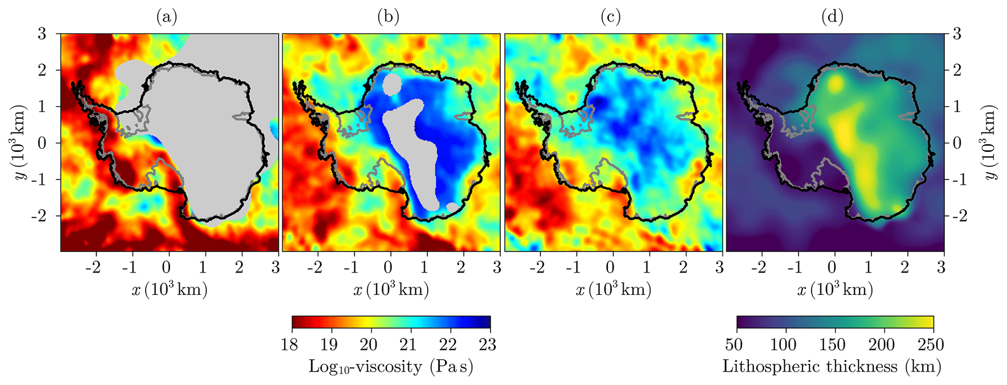
Figure 2 (a–c) Upper-mantle viscosity from Whitehouse et al. (2019) and Ivins et al. (2022) at 100, 200 and 300 km depth respectively. If the lithospheric thickness (Pan et al., 2022), depicted in (d), is larger than the layer depth, a grey shading is applied. The black and dark-grey contour lines respectively indicate the present-day ice-sheet and grounded-ice margins (Morlighem et al., 2020).

To tackle these issues, we propose FastIsostasy here, a regional 2D GIA model inspired by first principles and specially tailored for the needs of ice-sheet modellers. FastIsostasy (1) accounts for LV; (2) parameterises the depth dependence of the mantle viscosity; (3) captures the dependence of the response timescale on the mantle viscosity and the spatial scale of the load; (4) approximates the regional gravitation response and sea-level evolution; (5) is computationally inexpensive; (6) is extensively tested; and (7) offers a simple, open-source and extensively documented interface for a simplified coupling to an ice-sheet model. To illustrate its capabilities, Antarctica is used as a leitmotif of the present work since it displays (1) a high LV and depth dependence of solid-Earth properties as depicted in Fig. 2; (2) a high sensitivity to GIA due to the vast marine sectors of the AIS; (3) a large impact on the future of human societies due to possible rapid sea-level rise; and (4) large uncertainties in the solid-Earth parameters due, in part, to limited regional data sets. Antarctica might therefore be “the toughest test” when it comes to GIA modelling. Accordingly, the tools provided here are equally applicable to any other region covered by a past, present or future ice sheet.

1.4 FastIsostasy in the model hierarchy

The hierarchy of GIA models displays an important complexity gap between the computationally cheap models, which are largely used by the ice-sheet modelling community, and the computationally expensive models, developed by the GIA community. To give an impression of this, we herein present a brief overview, summarised in Tables 1 and 2, of the GIA model classes that are available to date and focus on the computation of the deformational response, with references to open-source implementations that we are aware of. The governing equations of the three first models can be found in Appendix A.

1.4.1 ELRA

The elastic lithosphere–relaxed asthenosphere (ELRA; Le Meur and Huybrechts, 1996) model conceptualises the structure of the solid Earth as two layers stacked along the depth dimension of a Cartesian coordinate system, obtained by a regional projection of the spherical Earth. The elastic lithosphere is parameterised by its constant thickness $T(x,y)=T$ and undergoes instantaneous compression under the effect of a load. It is underlain by the asthenosphere,² idealised as a viscous half-space parameterised by a constant relaxation time $\mathit{\tau }(x,y)=\mathit{\tau }$. According to this, the vertical displacement exponentially converges to the equilibrium solution, which is computed by convolving the load with a Green’s function. Parameterising the transient behaviour with a relaxation time is however simplistic, since, in reality, the response timescale of the solid Earth depends not only on the viscosity but also on the wavelength of the load, as mentioned previously. Furthermore, ELRA does not represent the depth dependence of the mantle viscosity or any LV. Due to its 2D regional domain, it ignores the gravitational and rotational feedbacks on the sea level, as well as the pre-stress and self-gravitation (Purcell, 1998) – the latter being partly cancelled by the lack of sphericity (Amelung and Wolf, 1994). Konrad et al. (2014) demonstrated that ELRA displays important transient differences to a 1D GIA model as well as discrepancies in the representation of the peripheral forebulge. Despite these numerous flaws, ELRA – or even simplified versions of it – remains a widespread choice among ice-sheet modellers (DeConto and Pollard, 2016; Lipscomb et al., 2019; Pattyn, 2017; Quiquet et al., 2018; Robinson et al., 2020; Rückamp et al., 2019), as it mimics the viscoelastic behaviour of the solid Earth with little implementation effort and at low computational cost. Its simplicity has led to a large number of implementations within open-source ice-sheet models (e.g. Lipscomb et al., 2019; Robinson et al., 2020), but, to our knowledge, no modular implementation is available to date. Ice-sheet modellers have therefore repeatedly spent time implementing ELRA, possibly with suboptimal computational performance, as it does not represent the primary focus of their work.

1.4.2 ELVA

This modelling approach was proposed by Cathles (1975), applied to ice-sheet modelling for the first time by Lingle and Clark (1985), and efficiently implemented by Bueler et al. (2007) through a Fourier collocation method (FCM). Although this model is sometimes named after the authors of the aforementioned work, we try to provide a unifying terminology here and therefore call it elastic lithosphere–viscous mantle (ELVA). ELVA resembles ELRA in its structure but is parameterised by the spatially homogeneous upper-mantle viscosity $\mathit{\eta }(x,y)=\mathit{\eta }$. It thus avoids any conversion from viscosity to relaxation time and allows for the mechanical response to depend on the wavelength of the load (Bueler et al., 2007). Furthermore, it permits embedding more of the radial structure of the mantle viscosity by introducing a viscous channel between the elastic plate and the viscous half-space.³ However, it does not address any other limitation of ELRA. It is worth mentioning that PISM (Winkelmann et al., 2011) provides an open-source implementation of ELVA, which is however embedded within a larger code base. This lack of modularity is addressed by giapy (Kachuck, 2017), a Python implementation of ELVA that might be more accessible than code traditionally written in Fortran or C$++$. ELVA was used, for example, by Kachuck et al. (2020) and Book et al. (2022) to study the stabilising potential of rapid bedrock uplift on the WAIS grounding-line retreat.

1.4.3 LV-ELRA

The laterally variable ELRA (LV-ELRA) proposed by Coulon et al. (2021) is a generalisation of ELRA to include laterally variable upper-mantle relaxation time τ(x,y) and lithospheric thickness T(x,y). The equilibrium displacement is obtained by solving equations derived from thin-plate theory (Ventsel and Krauthammer, 2001), which requires the use of finite-difference methods (FDMs) and is computationally more expensive than ELRA, since a large system of linear equations needs to be solved. To obtain τ(x,y), Coulon et al. (2021) apply a Gaussian smoothing on a binary field, with $\mathit{\tau }(x,y)={\mathit{\tau }}_{\mathrm{1}}$ in East Antarctica and $\mathit{\tau }(x,y)={\mathit{\tau }}_{\mathrm{2}}$ in the rest of the domain. Since LV-ELRA does not include a lateral coupling between the transient behaviour of neighbouring cells, this smoothing ensures a certain spatial coherence when relaxing the displacement field to the equilibrium solution; i.e. neighbouring cells have similar timescales. In addition to the limitations mentioned in Sect. 1.3, this coupling prevents the representation of very localised features, depicted in Fig. 2 and inferred in many studies (e.g. Barletta et al., 2018; Heeszel et al., 2016; Nield et al., 2014). In the rest of the paper, we will refer to these limitations as the ones resulting from a relaxed rheology.

Although computing the changes in SSH resulting from changes of Earth's gravity field requires, a priori, a global domain, it can also be approximated on a regional one. This was done by Coulon et al. (2021) and combined with LV-ELRA, resulting in the so-called elementary GIA model. This approach represents one of the most comprehensive regional GIA models developed to date and a valuable improvement for regional modelling, as it bypasses the computational expense of more complex models. The open-source ice-sheet model Kori includes the effort of Coulon et al. (2021), however not in a modular way that is directly usable to other ice-sheet modellers.

Konrad et al. (2014)Le Meur and Huybrechts (1996)Bueler et al. (2007)Kachuck et al. (2020)Book et al. (2022)Coulon et al. (2021)

Table 1 Comparison of the GIA models with 2D grids and low computational cost. L∈ℕ here denotes an arbitrary number of layers. Well-represented phenomena are represented by “✓”, and neglected ones are represented by “×”. Phenomena that are represented by a large amount of simplification are denoted by “≃”. For instance, LV-ELRA is here considered to only partially represent LV, since it is subject to the limitations of a relaxed rheology. Another example of partially represented phenomenon is the change in sea level, which typically requires a global domain but can be reasonably approximated regionally as done in the elementary GIA model and FastIsostasy (cf. Sect. 2.4).

1.4.4 Global 1D GIA models

Global 1D GIA models capture the radial structure of the solid Earth (down to the core–mantle boundary) but none of its lateral variability. They compute the gravitational field as well as the vertical and horizontal deformation by solving the underlying partial differential equations (PDEs) after spherical harmonic expansion of the dependent variables. The 1D GIA models typically represent the spatial heterogeneity of the SSH, the migration of shorelines and the rotational feedback (Kendall et al., 2005; Mitrovica and Milne, 2003; Spada and Melini, 2019). Most of them were cross-validated by Spada et al. (2011) and Martinec et al. (2018), showing great agreement while presenting intermediate computational cost. However, they are incapable of rendering any LV (e.g. Klemann et al., 2008). Spada and Melini (2019) proposed an open-source implementation of 1D GIA, which remains an exception in the field.

1.4.5 Regional 3D GIA models

Based on finite-element methods (FEMs), Nield et al. (2018) and Weerdesteijn et al. (2023) have proposed regional models to compute the solid-Earth deformation in the presence of LV. Unlike ELRA, ELVA and LV-ELRA, these regional GIA models resolve the depth dimension (down to the core–mantle boundary) and allow for grid refinement in regions where a higher resolution is needed. In particular, the work of Weerdesteijn et al. (2023) provides an open-source implementation that is compatible with heavily parallel hardware by extending ASPECT (Advanced Solver for Problems in Earth's ConvecTion), a model originally developed to solve mantle convection problems. Despite this, ASPECT requires about an hour to compute a few hundred years of high-resolution bedrock deformation on 256 CPUs. This represents a computational cost that is too high for most ongoing ice-sheet modelling studies, while ignoring the gravitational and rotational effects of GIA.

1.4.6 Global 3D GIA models

The 3D GIA models account for all the processes represented in 1D GIA models and are, in addition, capable of fully capturing the heterogeneity of solid-Earth properties. This also results in simulations that are more complicated to set up, since the user needs to provide fields of lithospheric thickness and mantle viscosity. Unlike 1D GIA models, 3D ones have not been systematically benchmarked but can be considered to be the best technology available for cases like Antarctica. In these models, the computation of the deformational response either relies on spherical harmonics (e.g. Bagge et al., 2021), FEM (e.g. A et al., 2013; Huang et al., 2023; Martinec, 2000; Sasgen et al., 2018; van der Wal et al., 2015; Wu, 2004; Zhong et al., 2022), the finite-volume method (FVM; Latychev et al., 2005; Gomez et al., 2018) or perturbation theory (e.g. Wu and Wang, 2006). Simulations on glacial timescales typically require at least several hours and up to few days (Albrecht et al., 2023; Pan et al., 2022; Zhong et al., 2022) of computation, even with heavily parallelised code. This is particularly problematic for propagating parametric uncertainties of the solid Earth on long simulations, since the limit of computational resources is typically reached with only one or a few ensemble members. As mentioned above, Zhong et al. (2022) proposed the first open-source implementation of a 3D GIA code.

Spada and Melini (2019)Nield et al. (2018)Weerdesteijn et al. (2023)Latychev et al. (2005)Zhong et al. (2022)

Table 2 Comparison of the GIA models with a 3D grid and higher computational cost. L∈ℕ here denotes an arbitrary number of layers. We focus on Maxwell rheology here, since it is most commonly used in the literature. However, these models can also be adapted to represent other rheologies.

1.4.7 FastIsostasy

The summary above points out a gap between the elementary GIA model (Coulon et al., 2021) and regional 3D GIA models (Nield et al., 2018; Weerdesteijn et al., 2023): the former is computationally cheap but suffers the limitation of a relaxed rheology, whereas the latter accurately represent the viscoelastic response of the solid Earth but come with a computational cost that makes them impractical for most ice-sheet modelling studies. FastIsostasy fills this gap by relying on LV-ELVA, a laterally variable generalisation of ELVA, coupled to a regional sea-level model (ReSeLeM), both of which are introduced in Sect. 2, along with a discussion of the underlying limitations. In Sect. 3, we discuss the practical features of its Julia implementation, such as the adaptive time stepping used for integration and GPU support. In Sect. 4, we subsequently benchmark FastIsostasy against analytical, as well as 1D and 3D numerical, solutions. Finally, we discuss the results as well as possible future improvements.

Remarks on open-source code. Thanks to recent work, the GIA model classes listed above now present at least some open-source code, which has typically become available much later than the first equivalent piece of proprietary code. For instance, 1D and 3D GIA models have already existed for 40 and 20 years respectively, but their first open-source implementations were only published much later, in respectively Spada and Melini (2019) and Zhong et al. (2022). We specifically refer here to source code that is licensed and can be downloaded and used without request. However, all open-source code mentioned above lacks tools from modern software development, including (1) dynamically built documentations with code examples; (2) automated test suites; and (3) a transparent development, which can be eased, for instance, by the use of GitHub issues and pull requests. Although these aspects are of a technical nature, we believe that they can make GIA models more user-friendly and their development more transparent, participative and reliable. This, in turn, reduces barriers in future research, and we have therefore applied these concepts to FastIsostasy.

Since LV-ELVA is a generalisation of ELVA, the latter can be used in FastIsostasy by simply providing it with homogeneous parameter fields. Additionally, we implemented ELRA in an efficient way, further described in Appendix A. Thus, both of these simpler models now present a modular, optimised and documented implementation, distributed under the GNU General Public License v3.0.

2 Model description

2.1 Preliminary considerations

As depicted in Fig. 3, FastIsostasy assumes a rectangular domain Ω⊂ℝ², obtained from a projection of the spherical Earth onto a Cartesian plane with dimensions 2 W_x and 2 W_y, in the directions of the lateral coordinates x and y respectively. We introduce the uniform spatial discretisation step $h_x=h_y=h$ such that the domain is subdivided into N_x×N_y cells, with $N_x,N_y\in \mathbb{N}$. We define all variables that are not specified as scalars (cf. Table 3) to be smooth fields, such as, for instance, the vertical load ${\mathit{\sigma }}^{zz}(x,y,t):{\mathbb{R}}^{\mathrm{3}}\to \mathbb{R}$. For convenience, we will omit the space and time dependence from now on. The discretised equivalent of smooth fields is denoted by bold symbols, e.g. ${\mathit{\sigma }}^{zz}\in {\mathbb{R}}^{N_x\times N_y}$, with their entries denoted by the index notation ${\mathit{\sigma }}_{i,j}^{zz}$, with $i\in \mathit{\{}\mathrm{1},\mathrm{2},\mathrm{\dots },N_x\mathit{\}}$, $j\in \mathit{\{}\mathrm{1},\mathrm{2},\mathrm{\dots },N_y\mathit{\}}$. The vertical load field is expressed as

$$\begin{array}{}\text{(1)}& {\displaystyle }{\mathit{\sigma }}^{zz}=-g\left({\mathit{\rho }}^{\mathrm{ice}}\mathrm{\Delta }{H}^{\mathrm{ice}}+{\mathit{\rho }}^{\mathrm{sw}}\mathrm{\Delta }{H}^{\mathrm{sw}}+{\mathit{\rho }}^{\mathrm{sed}}\mathrm{\Delta }{H}^{\mathrm{sed}}\right),\end{array}$$

with g as the mean gravitational acceleration at Earth's surface and ρ^ice, ρ^sw and ρ^sed as the mean densities of ice, seawater and sediment respectively.⁴ The height anomalies ΔH^ice, ΔH^sw and ΔH^sed of the corresponding columns are defined with respect to a reference state. On this domain, the first and second spatial derivatives of an arbitrary field M can be computed with central differences:

$$\begin{array}{}\text{(2)}& \begin{array}{ll}{\mathcal{D}}_x{M}_{i,j}& ={\displaystyle \frac{M_{i+\mathrm{1},j}-M_{i-\mathrm{1},j}}{\mathrm{2}h{K}_{i,j}}},\\ {\mathcal{D}}_y{M}_{i,j}& ={\displaystyle \frac{M_{i,j+\mathrm{1}}-M_{i,j-\mathrm{1}}}{\mathrm{2}h{K}_{i,j}}},\\ {\mathcal{D}}_{xx}{M}_{i,j}& ={\displaystyle \frac{M_{i+\mathrm{1},j}-\mathrm{2}{M}_{i,j}+M_{i-\mathrm{1},j}}{h^{\mathrm{2}}\cdot K_{i,j}^{\mathrm{2}}}},\\ {\mathcal{D}}_{yy}{M}_{i,j}& ={\displaystyle \frac{M_{i,j+\mathrm{1}}-\mathrm{2}{M}_{i,j}+M_{i,j-\mathrm{1}}}{h^{\mathrm{2}}\cdot K_{i,j}^{\mathrm{2}}}},\\ {\mathcal{D}}_{xy}{M}_{i,j}& ={\mathcal{D}}_y\left({\mathcal{D}}_x{M}_{i,j}\right),\end{array}\end{array}$$

with K as the distortion factor of the chosen projection.⁵ Furthermore, the pseudo-differential operator $\left|\mathrm{\nabla }\right|$ of an arbitrary matrix M is adapted from Bueler et al. (2007) to suit distorted grids:

$$\begin{array}{}\text{(3)}& \left|\mathrm{\nabla }\right|\mathbf{M}={\mathcal{F}}^{-\mathrm{1}}\left(\mathit{\kappa }\odot \mathcal{F}\left(\mathbf{M}\right)\right)\oslash \mathbf{K},\end{array}$$

with ⊙ as the element-wise product, ⊘ as the element-wise division, ℱ as the Fourier transform, ℱ⁻¹ as its inverse and κ as the coefficient matrix derived in Bueler et al. (2007). Models that do not account for distortion underestimate the length and area of cells away from the reference latitude and therefore require a domain with restricted spatial extent, a limitation that is overcome here.

Table 3 Numerical values of constants in FastIsostasy, from left to right: Earth's mass, Earth's radius, mean gravitational acceleration at Earth's surface, density of ice, sea water, lithosphere and mantle, elastic modulus and Poisson ratio of the lithosphere (compressible), and present-day ocean surface area. Values for the solid Earth are largely derived from the Preliminary Reference Earth Model (PREM; Dziewonski and Anderson, 1981) and the ocean surface from Cogley (2012).

Figure 3 Schematic representation of a typical FastIsostasy domain.

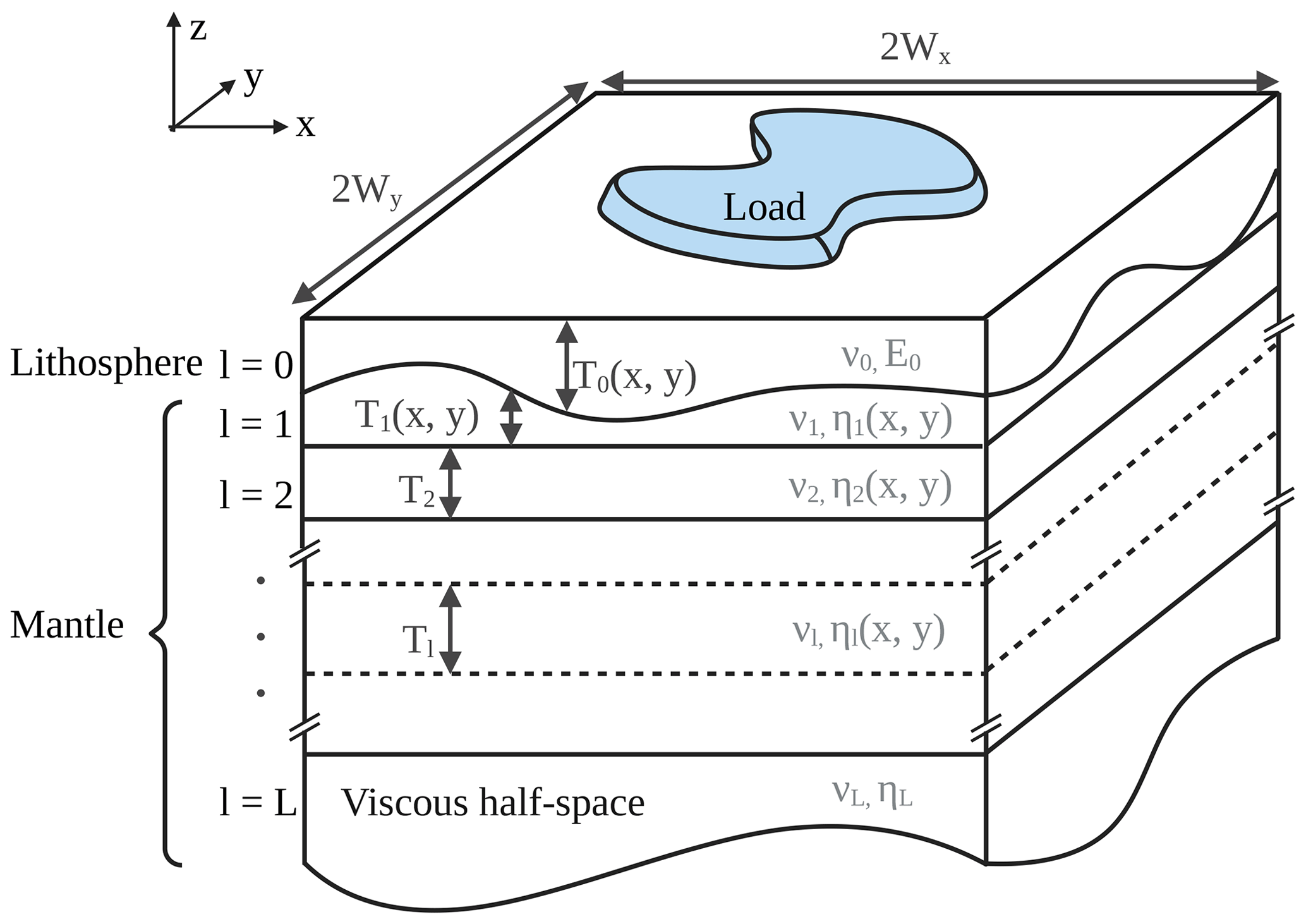
2.2 Lumping the depth dimension

As depicted in Fig. 3, the vertical structure of the solid Earth is modelled by a stack of layers along the vertical dimension z. With the layer index $l\in \mathit{\{}\mathrm{0},\mathrm{1},\mathrm{\dots },L-\mathrm{1},L\mathit{\}}$ going from top to bottom, the layers are the following:

• l=0 – an elastic plate with a laterally constant Young modulus $E_{\mathrm{0}}(x,y)=E_{\mathrm{0}}$ and Poisson ratio ${\mathit{\nu }}_{\mathrm{0}}(x,y)={\mathit{\nu }}_{\mathrm{0}}$ and laterally variable thickness T₀(x,y);

• $l\in \mathit{\{}\mathrm{1},\mathrm{2},\mathrm{\dots },L-\mathrm{2},L-\mathrm{1}\mathit{\}}$ – an arbitrary number of viscous channels, each with laterally constant Young modulus $E_l(x,y)=E_l$, Poisson ratio ${\mathit{\nu }}_l(x,y)={\mathit{\nu }}_l$ and laterally variable viscosity η_l(x,y) (as depicted in Fig. 3, the first of these layers has a laterally variable thickness T₁(x,y) that is complementary to T₀(x,y) and allows for all further layers to have a homogeneous $T_l(x,y)=T_l$ for l≥2);

• l=L – a viscous half-space with a laterally constant Young modulus $E_L(x,y)=E_L$, Poisson ratio ${\mathit{\nu }}_L(x,y)={\mathit{\nu }}_L$ and viscosity ${\mathit{\eta }}_L(x,y)={\mathit{\eta }}_L$.

Whereas l=0 represents the lithosphere, all further layers represent the remaining mantle. FastIsostasy lumps the latter layers into a single layer by computing a so-called effective viscosity for the whole mantle. The key to do so is provided by Cathles (1975), where a three-layer model including an elastic plate, a viscous channel and a viscous half-space is converted into a two-layer model where the viscous channel and the viscous half-space have been lumped into a single half-space by introducing the following scaling factor:

$$\begin{array}{}\text{(4)}& \begin{array}{rl}& R(\mathit{\kappa },\stackrel{\mathrm{̃}}{\mathit{\eta }},T)=\\ & {\displaystyle \frac{\mathrm{2}\stackrel{\mathrm{̃}}{\mathit{\eta }}CS+\left(\mathrm{1}-{\stackrel{\mathrm{̃}}{\mathit{\eta }}}^{\mathrm{2}}\right)T^{\mathrm{2}}{\mathit{\kappa }}^{\mathrm{2}}+{\stackrel{\mathrm{̃}}{\mathit{\eta }}}^{\mathrm{2}}{S}^{\mathrm{2}}+C^{\mathrm{2}}}{\left(\stackrel{\mathrm{̃}}{\mathit{\eta }}+{\stackrel{\mathrm{̃}}{\mathit{\eta }}}^{-\mathrm{1}}\right)CS+\left(\stackrel{\mathrm{̃}}{\mathit{\eta }}-{\stackrel{\mathrm{̃}}{\mathit{\eta }}}^{-\mathrm{1}}\right)T\mathit{\kappa }+S^{\mathrm{2}}+C^{\mathrm{2}}}},\end{array}\end{array}$$

with T as the channel thickness, $\stackrel{\mathrm{̃}}{\mathit{\eta }}$ as the channel viscosity divided by the half-space viscosity, C=cosh (Tκ) and S=sinh (Tκ). The characteristic wavenumber $\mathit{\kappa }=\mathit{\pi }{\mathit{\lambda }}^{-\mathrm{1}}$ is defined by choosing a characteristic wavelength λ for the load. Hence, solving the three-layer case can be formulated as solving the two-layer case with the half-space viscosity scaled by R. We propose generalising this idea by performing an induction from the bottom to the top layers, i.e. with decreasing l.

Initialisation. Layer l=L is a viscous half-space with ${\mathit{\eta }}_l^{\mathrm{eff}}={\mathit{\eta }}_L$.

Induction step. Layer l+1 can be represented as a viscous half-space with ${\mathit{\eta }}_{l+\mathrm{1}}^{\mathrm{eff}}$ and is overlain by a viscous channel l. These can be converted in an equivalent half-space with effective viscosity:

$$\begin{array}{}\text{(5)}& {\mathit{\eta }}_l^{\mathrm{eff}}=R\left(\mathit{\kappa },{\displaystyle \frac{{\mathit{\eta }}_l}{{\mathit{\eta }}_{l+\mathrm{1}}^{\mathrm{eff}}}},T_l\right)\cdot {\mathit{\eta }}_{l+\mathrm{1}}^{\mathrm{eff}}.\end{array}$$

Thus, ${\mathit{\eta }}_{\mathrm{1}}^{\mathrm{eff}}$ is the effective viscosity of the half-space representing the compound of layers $l\in \mathit{\{}\mathrm{1},\mathrm{2},\mathrm{\dots },L-\mathrm{1},L\mathit{\}}$. In essence, this represents a nonlinear mean of the viscosity over an arbitrary number of layers, which is only computed at initialisation and can improve the parameterisation of the depth dimension compared, for instance, to Bueler et al. (2007). However, this approach presents important limitations.

• Since the depth dimension is not resolved, the multi-modal response of Earth to surface loading is not captured as accurately as in 1D and 3D GIA models. For instance, the larger the load, the deeper the deformation into the mantle and the more relevant the radial layering of viscosity and density, which is not captured in FastIsostasy.

• The deformational response is likely to be less accurate for loads with dimensions that substantially differ from the characteristic wavelength λ, used in Eq. (4) to lump the depth dimension. We however emphasise that, for a given ice sheet, λ can be chosen such that the near field of deformation is represented well, which is typically what is required in simulations coupled to ice-sheet models. For all the computations presented here, we choose λ to be the mean of {W_x,W_y}.

• Equation (4), as derived in Cathles (1975), applies to laterally constant viscosities. In the present case, we however allow for the viscosity to be laterally variable and apply this scaling for each column.

Finally, to account for compressibility and lateral variations in the shear modulus, a scaling α of the viscosity is introduced and described in Appendix C. This yields the corrected effective viscosity η, which brings the Maxwell time of FastIsostasy close to that of a 3D GIA model:

$$\begin{array}{}\text{(6)}& \mathit{\eta }=\mathit{\alpha }{\mathit{\eta }}_{\mathrm{1}}^{\mathrm{eff}}.\end{array}$$

Although converting the 3D problem into a 2D one introduces the limitations mentioned above, it also greatly reduces the computational cost. In addition, the partial differential equation (PDE) governing an elastic plate on a viscous half-space can be transformed into an ordinary differential equation (ODE), as we describe in the next section.

2.3 LV-ELVA

We now assume that the aforementioned lumping of the layers has been performed and that the lithosphere and underlying mantle are represented by an elastic plate overlaying a viscous half-space. Since the vertical extent of the plate is typically 2 orders of magnitude smaller than its horizontal one, it is considered to be thin. By assuming a Maxwell rheology, the total vertical displacement u^el+u of the bedrock resulting from stress σ^zz can be decomposed in an elastic and a viscous response respectively denoted by u^el and u. As in Bueler et al. (2007), the elastic response of the lithosphere is computed by a convolution of the load σ^zz with an appropriate Green's function Γ^el:

$$\begin{array}{}\text{(7)}& u^{\mathrm{el}}={\mathrm{\Gamma }}^{\mathrm{el}}\otimes {\displaystyle \frac{K^{\mathrm{2}}{\mathit{\sigma }}^{zz}}{g}}.\end{array}$$

This represents the instantaneous compression of the lithosphere and accounts for the distortion resulting from the projection. In reality, this process takes place on the timescale of days, but it can be considered to be instantaneous compared to the long timescales of the viscous response and the ice-sheet dynamics. To construct the elastic Green's function, a “Gutenberg–Bullen A” spherical Earth model is assumed, and values from Farrell (1972, Table A3) are used, as done by Bueler et al. (2007). This treatment of the elastic response shows great agreement with a 3D GIA model, as shown in Sect. 4.

When material from the solid Earth is displaced, a hydrostatic force counteracting the load arises. We define the pressure field p as the sum of all these effects:

$$\begin{array}{}\text{(8)}& p={\mathit{\sigma }}^{zz}-g\left({\mathit{\rho }}^{\mathrm{l}}{u}^{\mathrm{el}}+{\mathit{\rho }}^{\mathrm{m}}u\right),\end{array}$$

with ρ^l and ρ^m as mean densities of the lithosphere and the upper mantle. Since the displacement occurs in Earth's outermost layers, we assume g to be constant over these shallow depths. The 3D GIA models usually represent the elastic lithosphere as a viscous layer with very high viscosity, and the elastic displacement therefore also implies a hydrostatic force. We argue that this is closer to reality and adapt this point of view to the present context by including the elastic displacement in Eq. (8), unlike Bueler et al. (2007) and Coulon et al. (2021). The evolution of the viscous displacement is therefore coupled to the elastic one and is governed by

$$\begin{array}{}\text{(9)}& \begin{array}{rl}& \mathrm{2}\mathit{\eta }(x,y)\left|\mathrm{\nabla }\right|\left({\displaystyle \frac{\partial u}{\partial t}}\right)=F\\ & F=p+{\displaystyle \frac{{\partial }^{\mathrm{2}}{M}_{xx}}{\partial x^{\mathrm{2}}}}+\mathrm{2}{\displaystyle \frac{{\partial }^{\mathrm{2}}{M}_{xy}}{\partial x\partial y}}+{\displaystyle \frac{{\partial }^{\mathrm{2}}{M}_{yy}}{\partial y^{\mathrm{2}}}},\end{array}\end{array}$$

with M_xx, M_yy and M_xy as the flexural moments for a thin plate (Coulon et al., 2021; Ventsel and Krauthammer, 2001):

$$\begin{array}{}\text{(10)}& {\displaystyle }{M}_{xx}=\underset{-T_{\mathrm{0}}/\mathrm{2}}{\overset{T_{\mathrm{0}}/\mathrm{2}}{\int }}{\mathit{\sigma }}^{xx}z\mathrm{d}z=-D\left({\displaystyle \frac{{\partial }^{\mathrm{2}}u}{\partial x^{\mathrm{2}}}}+\mathit{\nu }{\displaystyle \frac{{\partial }^{\mathrm{2}}u}{\partial y^{\mathrm{2}}}}\right),\text{(11)}& {\displaystyle }{M}_{yy}=\underset{-T_{\mathrm{0}}/\mathrm{2}}{\overset{T_{\mathrm{0}}/\mathrm{2}}{\int }}{\mathit{\sigma }}^{yy}z\mathrm{d}z=-D\left({\displaystyle \frac{{\partial }^{\mathrm{2}}u}{\partial y^{\mathrm{2}}}}+\mathit{\nu }{\displaystyle \frac{{\partial }^{\mathrm{2}}u}{\partial x^{\mathrm{2}}}}\right),\text{(12)}& {\displaystyle }{M}_{xy}=\underset{-T_{\mathrm{0}}/\mathrm{2}}{\overset{T_{\mathrm{0}}/\mathrm{2}}{\int }}{\mathit{\sigma }}^{xy}z\mathrm{d}z=-D(\mathrm{1}-\mathit{\nu }){\displaystyle \frac{{\partial }^{\mathrm{2}}u}{\partial x\partial y}}.\end{array}$$

In these equations, $D=E_{\mathrm{0}}{T}_{\mathrm{0}}^{\mathrm{3}}(x,y)\left(\mathrm{12}\right(\mathrm{1}-{\mathit{\nu }}_{\mathrm{0}}^{\mathrm{2}}){)}^{-\mathrm{1}}$ is the laterally variable lithospheric rigidity field. The PDE can be understood as an ad hoc generalisation of ELVA (Bueler et al., 2007; Cathles, 1975; Lingle and Clark, 1985) that is inspired by LV-ELRA (Coulon et al., 2021) and further described in Appendix A. Though we did not manage to formally derive it by generalising the work of Cathles (1975) to heterogeneous viscosities, Eq. (9) yields results that are very close to those of a 3D GIA model, as shown in Sect. 4. F on the right-hand side of the PDE can be evaluated by finite differences, as defined in Eq. (2):

$$\begin{array}{}\text{(13)}& \mathbf{F}=\mathbf{p}+{\mathcal{D}}_{xx}{\mathbf{M}}_{xx}+\mathrm{2}{\mathcal{D}}_{xy}{\mathbf{M}}_{xy}+{\mathcal{D}}_{yy}{\mathbf{M}}_{yy}.\end{array}$$

Subsequently, a Fourier collocation of this equation can be achieved by making use of Eq. (3) and rearranging terms:

$$\begin{array}{}\text{(14)}& {\displaystyle \frac{\partial \mathbf{u}}{\partial t}}={\mathcal{F}}^{-\mathrm{1}}\left(\mathcal{F}(\mathbf{F}\odot \mathbf{K}\oslash \mathrm{2}\mathit{\eta })\oslash \left(\mathit{\kappa }+\mathit{\epsilon }\right)\right),\end{array}$$

with ε≪1 as a regularisation term to avoid division by 0. Thus, by using a hybrid FDM–FCM approach the PDE expressed in Eq. (9) is transformed into an ODE, which can be solved with explicit integration methods. In particular, we thus avoid solving a large system of linear equations, as normally done in FDM, FVM or FEM code. Note that in Bueler et al. (2007) the closed form of a Crank–Nicolson (implicit) scheme is derived, thus providing unconditional stability. Due to the complexity of the right-hand side, finding such a closed form for LV-ELVA is more challenging and goes beyond the scope of this work. We emphasise that the smaller time steps resulting from explicit schemes might nevertheless be needed for (1) coupling purposes, as a dense output in time can be provided to the ice-sheet model, and (2) accurately capturing the fast dynamics that can occur in regions of low viscosity.

Far away from the ice sheet, the changes of the load are comparatively small, and we therefore require the displacement to be zero at the domain boundaries.⁶ However, FCM does not allow explicit treatment of Dirichlet boundary conditions (BCs). To enforce its approximate representation, we subtract the mean displacement of the corner vertices from the solution at each time step, which is here expressed with the common choice of notation from programming:

$$\begin{array}{}\text{(15)}& u_{i,j}:=u_{i,j}-{\displaystyle \frac{\mathrm{1}}{\mathrm{4}}}(u_{\mathrm{1},\mathrm{1}}+u_{\mathrm{1},N_y}+u_{N_x,\mathrm{1}}+u_{N_x,N_y}).\end{array}$$

Note that this differs from Bueler et al. (2007), where the whole domain boundary is used for this purpose. We argue that our approach is a better representation of the required BC because corner points are (1) further away from the load and (2) equidistant from the centre of a rectangular domain.

2.4 Regional sea-level model (ReSeLeM)

In a coupled setting, a GIA model is typically expected to take the ice thickness field as an input and to return the RSL field S as an output, which can be expressed as

$$\begin{array}{}\text{(16)}& {\displaystyle }S(x,y,t)=z^{\mathrm{ss}}(x,y,t)-z^{\mathrm{b}}(x,y,t),\text{(17)}& {\displaystyle }{z}^{\mathrm{ss}}(x,y,t)=s\left(t\right)+N(x,y,t)+c\left(t\right),\text{(18)}& {\displaystyle }{z}^{\mathrm{b}}(x,y,t)=z_{\mathrm{ref}}^{\mathrm{b}}(x,y)+u(x,y,t)+u^{\mathrm{el}}(x,y,t),\end{array}$$

with z^ss as the SSH, z^b as the bedrock elevation, s as the barystatic sea level (BSL), N as the SSH perturbation due to changes in the gravitational field and c as a time-dependent scalar. In a global model, c ensures mass conservation of water, which is however impossible to ensure in a regional model with open boundaries. In contrast, we use c to impose a mean zero SSH perturbation at the domain boundary, similar to Eq. (15). The sea-level terminology used here follows the definitions of Gregory et al. (2019), which we refer to for any further detail. Whereas the displacements u and u^el are computed as described in Sect. 2.3, the SSH perturbation N can be regionally approximated by the convolution of the mass anomaly with an appropriate Green's function Γ^N, as proposed in Coulon et al. (2021):

$$\begin{array}{}\text{(19)}& {\displaystyle }N={\mathrm{\Gamma }}^N\otimes {\displaystyle \frac{K^{\mathrm{2}}p}{g}},\text{(20)}& {\displaystyle }{\mathrm{\Gamma }}^N\left(\mathit{\theta }\right)={\displaystyle \frac{R_{\mathrm{e}}}{M_{\mathrm{e}}}}\left({\displaystyle \frac{\mathrm{1}}{\mathrm{2}\sin (\mathit{\theta }/\mathrm{2})}}\right),\end{array}$$

with R_e as Earth's radius at the Equator, M_e as Earth's mass and θ as the colatitude. To avoid dividing by θ=0°, we impose a minimal colatitude of the order of the resolution. By neglecting the changes in surface load from sediments and expressing ΔH^sw with the RSL, Eq. (1) becomes

$$\begin{array}{}\text{(21)}& {\displaystyle }{\mathit{\sigma }}^{zz}=-g\mathcal{A}({\mathit{\rho }}^{\mathrm{sw}}\mathrm{\Delta }S\mathcal{O}+{\mathit{\rho }}^{\mathrm{ice}}\mathrm{\Delta }{H}^{\mathrm{ice}}\mathcal{C}),\text{(22)}& {\displaystyle }\mathrm{\Delta }S=S-S_{\mathrm{ref}},\text{(23)}& {\displaystyle }\mathrm{\Delta }{H}^{\mathrm{ice}}=H^{\mathrm{ice}}-H_{\mathrm{ref}}^{\mathrm{ice}},\end{array}$$

with 𝒪 as the ocean function; 𝒞 as the continent function; and 𝒢 as the grounded-ice function, which can be expressed by introducing the indicator function 𝟙 and the ice thickness above flotation H^af:

$$\begin{array}{}\text{(24)}& {\displaystyle }\mathcal{O}=\mathrm{1}-max(\mathcal{C},\mathcal{G}),\text{(25)}& {\displaystyle }\mathcal{C}=\text{𝟙}(S<\mathrm{0}),\text{(26)}& {\displaystyle }\mathcal{G}=\text{𝟙}(H^{\mathrm{af}}>\mathrm{0}),\text{(27)}& {\displaystyle }{H}^{\mathrm{af}}=H^{\mathrm{ice}}-S{\displaystyle \frac{{\mathit{\rho }}^{\mathrm{ice}}}{{\mathit{\rho }}^{\mathrm{sw}}}}.\end{array}$$

In Eq. (21), the activation mask 𝒜 defines what we further consider the near field of displacement: it yields 1 close to the ice sheet and 0 otherwise. This approach is similar to what is done in Coulon et al. (2021) and is, by definition, somewhat arbitrary. The choice made here is illustrated in Sect. 4 for Antarctica. Most importantly, the activation mask enforces a zero change in load close to the boundary of the domain, which is necessary to fulfil the BCs expressed in Eq. (15). This is a limitation compared to a global GIA model but allows for accounting for water column changes in the near field of the ice sheet, unlike most regional models (Book et al., 2022; Bueler et al., 2007; Kachuck et al., 2020; Lingle and Clark, 1985; Le Meur and Huybrechts, 1996; Weerdesteijn et al., 2023).

In Goelzer et al. (2020), the evolution of the BSL is described as⁷

$$\begin{array}{}\text{(28)}& {\displaystyle }s\left(t\right)={\displaystyle \frac{V\left(t\right)}{A_{\mathrm{pd}}}},\text{(29)}& {\displaystyle }V\left(t\right)=V^{\mathrm{af}}\left(t\right){\displaystyle \frac{{\mathit{\rho }}^{\mathrm{ice}}}{{\mathit{\rho }}^{\mathrm{sw}}}}+V^{\mathrm{pov}}\left(t\right)+V^{\mathrm{den}}\left(t\right),\end{array}$$

with A_pd as the present-day ocean surface and V as the volume contribution of ice sheets to the ocean. The latter is decomposed into V^af, the contribution from ice above flotation; V^pov, the contribution from changes in the bedrock height; and V^den, the contribution from density differences between meltwater and seawater. We refer the reader to Goelzer et al. (2020) for the detailed computation of these quantities, which are defined with respect to a reference state, typically the present-day one. Assuming a fixed ocean surface to compute the evolution of the sea level can, however, lead to a bias of tens of metres over glacial cycles. To tackle this, we propose an extension of Goelzer et al. (2020) that accounts for the time dependence of the ocean surface A(t) when computing the BSL. To this end, we first introduce a time discretisation t=k Δt, with 𝒪(Δt)=10 years. We further introduce the ocean surface as a function A(s), which is nonlinear with respect to the BSL s when a realistic topography is used, as shown in Fig. 4 and described with more detail in Sect. B. The volume change $\mathrm{\Delta }{V}_k=V_k-V_{k-\mathrm{1}}$ over a time step leads to a change $\mathrm{\Delta }{s}_k={\mathrm{s}}_k-{\mathrm{s}}_{k-\mathrm{1}}$ of the BSL. Since Δt is much smaller than glaciological timescales, Δs_k is a small number and the nonlinear relationship between the volume contribution, the ocean surface and the BSL can be approximated by a trapezoidal rule, pictured in Fig. 4 and described by the following equation:

$$\begin{array}{}\text{(30)}& \mathrm{\Delta }{V}_k=(s_k-s_{k-\mathrm{1}}){\displaystyle \frac{A\left(s_k\right)+A\left(s_{k-\mathrm{1}}\right)}{\mathrm{2}}}.\end{array}$$

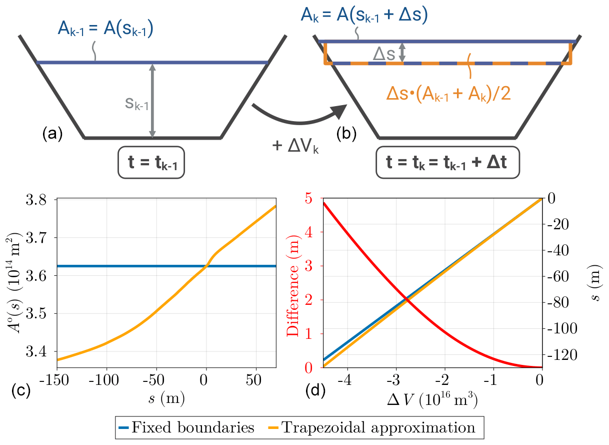
Figure 4 (a, b) Schematic representation of the trapezoidal approximation used to solve the nonlinear dependence between BSL s and ocean surface A. We hereby use A_k as shorthand for A(s_k). (c) Present-day ocean surface and ocean-surface function A(s) as computed by the trapezoidal approximation of the basin evolution. (d) BSL computed for a change in ice volume equivalent to the LGM, for fixed boundaries compared to the trapezoidal approximation.

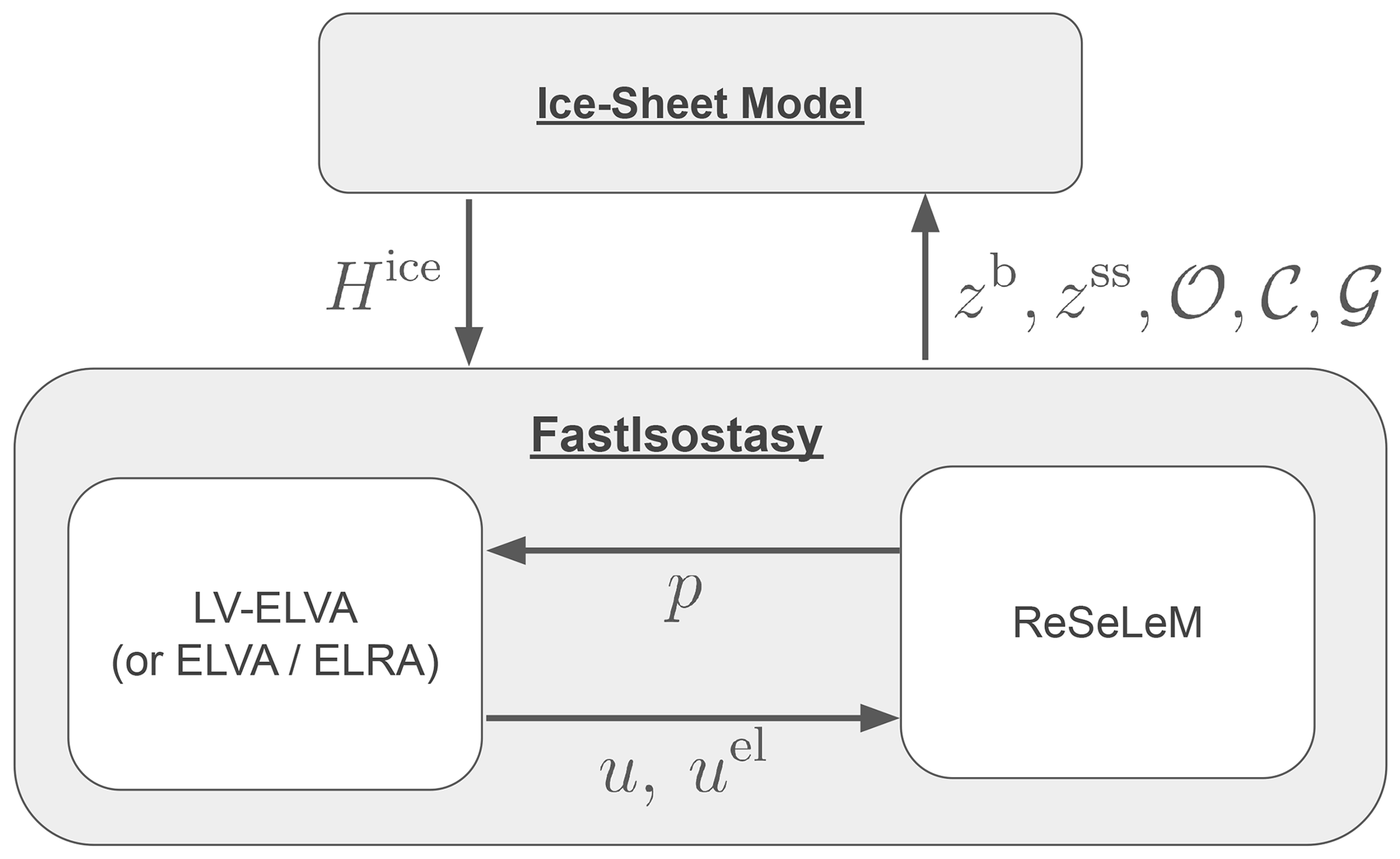
Figure 5 Interface between FastIsostasy and an ice-sheet model, adapted from De Boer et al. (2017) and Coulon et al. (2021).

Equation (30) is solved by using s_k−1 as an initial guess, and the updated BSL s_k is typically obtained after a few iterations of the nonlinear solver. This is of course an important simplification compared to global GIA models, which typically resolve the migration of shorelines (Kendall et al., 2005; Mitrovica and Milne, 2003). Nonetheless, this is an improvement compared to fixing A(t)=A_pd. In particular, Fig. 4d shows that the sea level of the Last Glacial Maximum (LGM) is overestimated by about 5 m for fixed ocean boundaries compared to our trapezoidal approximation. This can lead to differences of several kilometres in the grounding-line position, depending on the local bedrock slope. We emphasise that a more sophisticated approach than ours is likely to require a global domain, which we want to avoid here.

In summary, allowing for a time-variable ocean surface is the main adaptation of the sea-level treatment described in previous work (Coulon et al., 2021; Goelzer et al., 2020), and it constitutes ReSeLeM. FastIsostasy involves, as depicted in Fig. 5, a coupling between LV-ELVA and ReSeLeM.

2.5 Limitations

LV-ELVA presents limitations, since it relies on a linear PDE describing the macroscopic behaviour of the solid Earth as a Maxwell body. Therefore it does not account for transient rheologies (Caron et al., 2017; Ivins et al., 2021), nonlinear rheologies (Gasperini et al., 2004; Kang et al., 2021), composite rheologies (van der Wal et al., 2010, 2015), anisotropy (Accardo et al., 2014; Beghein et al., 2006) or microscale properties of the material (Van Calcar et al., 2023). LV-ELVA only computes the vertical displacement of GIA and neglects the horizontal one, which has a negligible impact on ice-sheet dynamics. Nonetheless, the horizontal displacement might be used to constrain GIA models through GNSS (global navigation satellite system) measurements, and its implementation is left for future versions of the model.

The governing equation of LV-ELVA was postulated here in an ad hoc way, as described in Sect. A, but lacks a formal derivation. Since the depth dimension is not resolved in LV-ELVA, Stokes flow of the mantle is not fully represented, similar to depth-integrated solvers of ice-sheet dynamics and shallow-water approximations used in general circulation models. In addition, the regional nature of the domain makes it inherently complicated to ensure BCs that are consistent with a global conservation of mass. Therefore, the sea level is only solved in an approximate way, and the feedback from perturbations in Earth's rotation, which will be small near the poles, is not accounted for. In particular, we emphasise that the update of the BSL described in Eq. (30) fails to give good results if most of the contribution stems from an ice sheet that is not included in the domain. For instance, the BSL computed in FastIsostasy over a glacial cycle cannot be correct if the domain only covers Antarctica, since most of the contribution stems from the Northern Hemisphere ice sheets. However, this can however be by setting up a domain for the Northern Hemisphere and coupling it to the Antarctic one or simply by taking the BSL obtained from proxies or global GIA models.

Future releases of FastIsostasy will focus on addressing some of these problems. We emphasise that, despite these limitations, the results presented in Sect. 4 show that FastIsostasy is a significant improvement compared to ELRA and ELVA, since it represents the near-field GIA response of laterally variable Earth structures with improved accuracy and a negligible increase in computational cost. We believe that this adequately covers the needs of most ice-sheet modellers.

3 Implementation, performance and further remarks

FastIsostasy has been implemented in Julia (FastIsostasy.jl) and in Fortran. Julia (Bezanson et al., 2017) is a high-performance language with a vast ecosystem, on which FastIsostasy.jl relies to offer convenient features and efficient computation.

1. To evaluate the right-hand side of the ODE obtained in Eq. (14) and perform the convolutions used to compute the elastic and the gravitational response, FastIsostasy.jl uses forward and inverse fast Fourier transforms (FFTs), which are implemented in an optimised way in FFTW.jl (Frigo and Johnson, 2005). Evaluating the right-hand side therefore scales with a computational complexity of 𝒪(N log ₂N), for a matrix of size $N=N_x\times N_y$. To achieve an even better speed increase, (1) N_x and N_y are generally chosen as powers of 2, (2) FFTs are precomputed as far as possible, and (3) the transforms are computed in place to reduce the memory allocation. FastIsostasy owes its name to fast-earth, an early implementation of ELVA (referred to in the Acknowledgements) and to its reliance on FFTs to perform all the expensive computations.

2. To subsequently integrate the right-hand side in time, FastIsostasy.jl uses OrdinaryDiffEq.jl (Rackauckas and Nie, 2017), a package that offers a wide range of optimised routines. We restrict ourselves here to explicit methods, which range from the simplest explicit Euler scheme up to schemes of order 14. For all the results presented here, we used the Runge–Kutta method proposed in Bogacki and Shampine (1996). Explicit integration schemes typically require decreasing the time step with increasing spatial resolution, which is handled by the adaptive time-stepping methods of OrdinaryDiffEq.jl to prevent instabilities. This requires more evaluations of the right-hand side and increases the computational complexity of the full problem to higher than 𝒪(N log ₂N). By providing keyword arguments, the user is able to influence any option related to the integration in time, such as the scheme, the error tolerance and the minimal time step.

3. FastIsostasy.jl uses CUDA.jl (Besard et al., 2019) and ParallelStencil.jl to optionally run performance-relevant computations on a GPU (so far restricted to NVIDIA hardware). Due to their heavily parallelised architecture, GPUs are able to scale better than CPUs for some computations. The speed increase thus obtained will be illustrated in Test 1 of the model validation. Offering a GPU-parallelised GIA code is unprecedented to our knowledge and only requires the user to set the keyword argument use_cuda=true.

4. In FastIsostasy.jl, the nonlinearity introduced by the time-dependent ocean surface is solved by using NLsolve.jl, in combination with an interpolation of A(s), which is constructed at initialisation using Interpolations.jl. Since A(s) is monotonic and initial guesses are close to the solution, the computation time associated with this step is negligible. Furthermore, whereas the adaptive time stepping is convenient for enforcing the stability of the viscous displacement, updating the diagnostics – such as the elastic displacement, the ocean surface and sea level – can be done less frequently. For instance Δt=10 years is used in the present work and can be determined by the user through a keyword argument.

As illustrated above, FastIsostasy.jl relies on numerous Julia packages. Since it is a registered package, it can however be easily installed, along with all its dependencies, by simply running add FastIsostasy in Julia's package manager. Furthermore, it is thoroughly documented at https://janjereczek.github.io/FastIsostasy.jl/dev/ (last access: 4 July 2024), including a description of the application programming interface; a tutorial; and practical examples, which are a simplified version of the code used for the results shown in Sect. 4. Additionally, FastIsostasy.jl is designed in a modular way that facilitates its coupling to an ice-sheet model, and we therefore believe that the implementation burden associated with its use is very low.

Since Julia does not yet support compilation to binaries, FastIsostasy is additionally programmed in Fortran to allow for compatibility with most existing ice-sheet models and has already been coupled to Yelmo (Robinson et al., 2020). Since Fortran does not provide packages that are as convenient as those of the Julia ecosystem, the Fortran version (1) does not allow for computation on a GPU, (2) only provides explicit Euler schemes for integration in time and (3) does not allow for time-evolving ocean boundaries.

Table 4 Summary of the tests performed using FastIsostasy. The two last columns provide tight upper bounds on the mean and maximal errors over space. The Antarctic LV used in Test 4 is the same as in Pan et al. (2022).

4 Model validation and benchmarks

We now validate FastIsostasy with series of tests.

• Test 1 is a comparison to an analytical solution for an idealised load on a homogeneous, flat Earth. This aims to check that the numerics are implemented well for the simplest case and that our results are comparable to Bueler et al. (2007).

• Test 2 is a comparison to benchmark solutions of three different 1D GIA models, presented in Spada et al. (2011). This aims to understand the discrepancies which can arise from the lumping of depth-dependent viscosity profiles and the regional approximations of the SSH perturbation.

• Test 3 is a comparison to the 3D GIA model Seakon (Gomez et al., 2018; Latychev et al., 2005) for idealised cases of LV. This aims to check whether Eq. (9) and its discretisation, Eq. (14), are valid approximations of the deformational response in the presence of LV. Here we will also compare the elastic displacement of Seakon and FastIsostasy.

• Test 4 is a comparison to Seakon with realistic LV and forced by the ice loading of a full glacial cycle. This aims to check whether loads and Earth structures of typical applications can be represented reasonably well.

These tests are summarised in Table 4 and aim to quantify, as independently as possible, each source of error between FastIsostasy and the baseline solutions listed above. This is measured by an absolute and a relative value respectively defined as

$$\begin{array}{}\text{(31)}& {\displaystyle }{e}^{\mathrm{abs}}(x,y,t)=\left|u_{\mathrm{FI}}\right(x,y,t)-u_{\mathrm{BL}}(x,y,t\left)\right|,\text{(32)}& {\displaystyle }e(x,y,t)={\displaystyle \frac{e^{\mathrm{abs}}(x,y,t)}{\underset{x,y,t}{max}\left|u_{\mathrm{BL}}\right(x,y,t\left)\right|}},\end{array}$$

with the indices “FI” and “BL” respectively indicating the FastIsostasy and baseline solutions. We refer to the mean and maximal errors over space as $\overline{e}\left(t\right)$ and $\widehat{e}\left(t\right)$. In the forthcoming analysis, we will often mention a tight upper bound for these time series to quantify them in a scalar way and will emphasise the maximal error, since the spatial mean can hide important local discrepancies.

4.1 Test 1 – analytical solution for an idealised load on a homogeneous Earth

We first reproduce the test proposed in Bueler et al. (2007) by using a two-layer model with $W_x=W_y=\mathrm{3000}$ km, $N=N_x=N_y=\mathrm{256}$ and h≃23 km. The first layer is parameterised by the lithospheric thickness $T(x,y)=\mathrm{88}$ km, and the underlying half-space is parameterised by the mantle viscosity $\mathit{\eta }(x,y)={\mathrm{10}}^{\mathrm{21}}$ Pa s. The load is a Heaviside function in time that represents a flat cylinder of ice, with radius R=1000 km and thickness H=1 km, placed at the centre of the computation domain. For this idealised case, an analytical solution of the viscous solution is provided in Bueler et al. (2007), yielding

$$\begin{array}{}\text{(33)}& {\displaystyle }u(r,t)={\mathit{\rho }}^{\mathrm{ice}}gHR\underset{\mathrm{0}}{\overset{\mathrm{\infty }}{\int }}\mathit{\psi }\left(\mathit{\kappa }\right)\mathrm{d}\mathit{\kappa },\text{(34)}& {\displaystyle }\mathit{\psi }\left(\mathit{\kappa }\right)={\mathit{\beta }}^{-\mathrm{1}}\left[\exp \left(-{\displaystyle \frac{\mathit{\beta }t}{\mathrm{2}\mathit{\eta }\mathit{\kappa }}}\right)-\mathrm{1}\right]J_{\mathrm{1}}\left(\mathit{\kappa }{R}_{\mathrm{0}}\right)J_{\mathrm{0}}\left(\mathit{\kappa }r\right),\end{array}$$

with J₀ and J₁ as the Bessel functions of the first kind and are respectively of order 0 and 1 and $\mathit{\beta }=\mathit{\beta }\left(\mathit{\kappa }\right)={\mathit{\rho }}^{\mathrm{m}}g+D{\mathit{\kappa }}^{\mathrm{4}}$. To make the solution of FastIsostasy comparable to this, we set K_i,j to 1 and ρ^l to 0, which neglects distortion and prevents the elastic displacement from contributing to the pressure term. Figure 6a shows cross-sections of the domain along the x dimension, demonstrating that the numerical solution closely follows the analytical one. Complementarily, Fig. 6b shows the corresponding maximal and mean error over time. For t≥5000 years, the viscous displacement is captured with ${\overline{e}}^{\mathrm{abs}}<{\widehat{e}}^{\mathrm{abs}}<\mathrm{1}$ m. For t≤2000 years, the displacement surface is well captured in terms of shape but appears to be slightly shifted along the z dimension due to the approximate treatment of the BCs as written in Eq. (15), leading to a larger upper bound on the error ${\widehat{e}}^{\mathrm{abs}}\left(t\right)<\mathrm{5.8}$ m, which corresponds to $\widehat{e}<\mathrm{0.021}$. Whereas in Bueler et al. (2007) a correction of this effect is applied based on the knowledge of the analytical solution, we decide not to do so here, first, because such a correction only applies to this specific case and, second, because users should be informed about the potential numerical error that will arise in their experiments. When imposing Eq. (15), the unrealistically high forcing rate resulting from the Heaviside load leads to errors that are higher than what is expected from a load that is coherent in time. The discretisation error presented here should be therefore understood as an upper bound for a flat Earth.

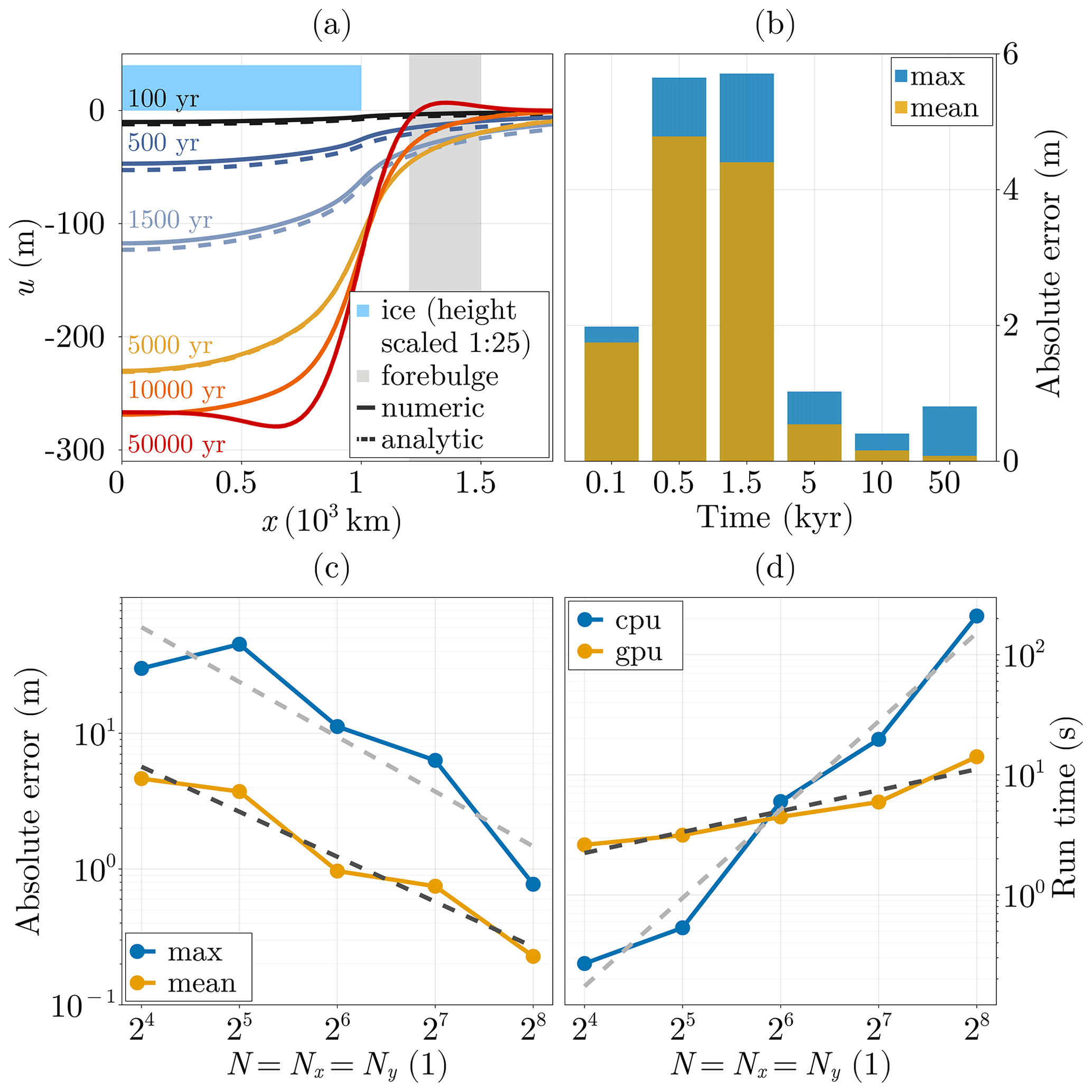
Figure 6 (a) Transient cross-sections of bedrock displacement along the x axis, from the centre of the domain until x=1800 km. The resolution used here is $N_x=N_y={\mathrm{2}}^{\mathrm{8}}$, with h≃23 km. (b) Corresponding mean and maximal errors over time. (c) Resolution dependence of the maximum and mean error at equilibrium with respect to the analytical solution, with the dashed light- and dark-grey lines representing the corresponding linear regressions respectively with slopes of −0.4 and −0.33 in log ₂−log ₁₀ space. (d) Resolution dependence of the computation time on a CPU versus a GPU, with the dashed light- and dark-grey lines representing the corresponding linear regressions respectively with slopes of 0.73 and 0.17 in log ₂−log ₁₀ space.

Figure 6c shows that the maximal and mean equilibrium error respectively decrease with a slope of −0.4 and −0.33 in log ₂−log ₁₀ space, showing that convergence to the analytical solution of equilibrium can be achieved relatively quickly with increasing resolution. The runtime on a CPU (Intel i7-10750H, 2.60 GHz) versus a GPU (NVIDIA GeForce RTX 2070) is depicted in Fig. 6d and shows that using a GPU is advantageous for N≥64, which corresponds to the typical problem size for ice-sheet modelling. More specifically, the CPU and GPU computation time respectively increase with a slope of 0.73 and 0.17 in log ₂−log ₁₀ space, thus giving a clear advantage to GPU computation for large problems. Thanks to the hybrid FDM–FCM scheme used to evaluate Eq. (14), the scaling of computation time on both a CPU and GPU is better than is usually obtained from FDM, FVM and FEM since all of them rely on solving a large system of linear equations.

4.2 Test 2 – 1D GIA solutions of idealised loads on a layered Earth

In Spada et al. (2011), a range of 1D GIA models are benchmarked against each other and show excellent agreement on various experiments. Here, we reproduce the benchmark tests called “1/2” (geodetic quantities) and “2/2” (geodetic rates), which are similar to Test 1 but present the following differences.

• The computation domain is a stereographic projection of the spherical Earth, centred at colatitude θ=0°, and the effect of distortion is therefore included, unlike for Test 1. We apply ice loads with ρ^ice=931 kg m⁻³, chosen in agreement with Spada et al. (2011), and the following geometries:

  • a.

    an ice cap with maximal height H_max=1.5 km, radius θ=10° and a shape defined by a cosine function;

  • b.

    a cylindrical ice load of thickness H=1 km and radius θ=10°,

• Earth's structure has three layers, namely (1) a lithosphere of thickness T₀=70 km and shear modulus $G_{\mathrm{0}}=\mathrm{5}\times {\mathrm{10}}^{\mathrm{11}}$ Pa, (2) an upper mantle of thickness T₁=600 km and viscosity η₁=10²¹ Pa s, and (3) a lower mantle reaching down to the core–mantle boundary with viscosity ${\mathit{\eta }}_{\mathrm{2}}=\mathrm{2}\times {\mathrm{10}}^{\mathrm{21}}$Pa s. For any further detail, we refer the reader to the M3-L70-V01 profile shown in Spada et al. (2011). In FastIsostasy, these layers are translated into an elastic plate, a viscous channel and a viscous half-space.

• The results of SSH perturbation provided in Spada et al. (2011) allow us to check the validity of Eq. (19), used in FastIsostasy.

Figure 7 Comparison of FastIsostasy and Spada et al. (2011) on tests $\mathrm{1}/\mathrm{2}$ and $\mathrm{2}/\mathrm{2}$. From top to bottom: viscous displacement u, viscous displacement rate $\dot{u}$ and the resulting SSH perturbation N. From left to right: cylinder and cap of ice applied as the load.

Figure 7 demonstrates that the viscous displacement, its rate and the SSH computed in FastIsostasy qualitatively follow the results of Spada et al. (2011). The latter corresponds to the outputs of PMTF, VILMA and VEENT, which show such a good agreement that they are gathered into a single output. Quantitatively, the mean displacement error between FastIsostasy and Spada et al. (2011) is small, with ${\overline{e}}^{\mathrm{abs}}\left(t\right)<\mathrm{27.0}$ m for both loading cases. In addition, the equilibrium displacement is represented well by a maximal error of ${\widehat{e}}^{\mathrm{abs}}(t=\mathrm{100}\mathrm{kyr})<\mathrm{7}$ m and ${\widehat{e}}^{\mathrm{abs}}(t=\mathrm{100}\mathrm{kyr})<\mathrm{12}$ m and a mean error of ${\overline{e}}^{\mathrm{abs}}(t=\mathrm{100}\mathrm{kyr})<\mathrm{5}$ m and ${\overline{e}}^{\mathrm{abs}}(t=\mathrm{100}\mathrm{kyr})<\mathrm{7}$ m, for the cap and the disc load respectively. The maximal difference arises at t=10 kyr for the cylindrical load and yields ${\widehat{e}}^{\mathrm{abs}}<\mathrm{47}$ m, i.e. $\widehat{e}<\mathrm{0.19}$. In both cases, the difference in vertical displacement is propagated to the computation of the SSH perturbation according to Eq. (19). As shown in the last row of Fig. 7, this leads to a maximal difference between FastIsostasy and the 1D GIA models that reaches at most 6 m but less than 2 m on average, for maximal SSH perturbations around 40 m in both models.

Since the experimental setup is as similar as possible for the 1D GIA models and FastIsostasy, these differences can be largely attributed to (1) the lumping of the depth dimension as performed in Eq. 4, which leads the two approaches to solve different equations, and (2) to the regional domain used here, which only allows for an approximate treatment of the BCs as described in Eq. (15).

4.3 Test 3 – 3D GIA solution of idealised load on an idealised LV Earth

Seakon is a global 3D GIA model that includes all the processes mentioned in Sect. 1.4.6. It solves the deformational response of the solid Earth with FVM on an unstructured grid, which is typically finer at the poles, where the bedrock displacement is largest. It has been extensively used in GIA studies (e.g.  Austermann et al., 2021; Mitrovica et al., 2009; Pan et al., 2021, 2022) and coupled to an ice-sheet model in Gomez et al. (2018). For further details about the model and the adaptive grid refinement, we refer the reader to Latychev et al. (2005) and Gomez et al. (2018). We benchmark FastIsostasy against Seakon here for idealised cases with LV similar to that estimated across Antarctica. Here again, a cylindrical ice load with H=1 km and R=1000 km is applied on a domain with $W_x=W_y=\mathrm{3000}$ km and $N_x=N_y=\mathrm{128}$. To isolate the error from the lumping of the depth dimension, the vertical structure of the solid Earth is kept as simple as possible, with a mantle viscosity that is constant along z.

We distinguish four cases (a–d), which are all parameterised by a Gaussian-shaped anomaly that is almost 0 on the boundary and yields its largest value at the interior of the domain. For case a (case b), this anomaly represents a decrease (increase) from T=150 km down to T=50 km (up to T=250 km) of the lithospheric thickness towards the interior of the domain. For case c (case d), this anomaly represents an exponential decrease (increase) from η=10²¹ Pa s down to η=10²⁰ Pa s (up to η=10²² Pa s) of the mantle viscosity towards the interior of the domain. The heterogeneities (a–d) are shown in Appendix D and are used to generate results that are referred to as “LV-ELVA”. To quantify the improvement resulting from the use of LV-ELVA instead of ELVA (or ELRA), we also generate results with the nominal, homogeneous parameters $T(x,y)=\mathrm{150}$ km and $\mathit{\eta }(x,y)={\mathrm{10}}^{\mathrm{21}}$ Pa s (or τ=3000 years) and index them with “ELVA” (or “ELRA”).

As can be seen in the top and middle row of Fig. 8, LV-ELVA closely follows Seakon on cases a–b by showing similar timescales, amplitudes and shapes of the bedrock displacement. In the bottom row of Fig. 8, the maximal and mean relative differences respectively remain at $\widehat{e}\left(t\right)<\mathrm{0.07}$ and $\overline{e}\left(t\right)<\mathrm{0.03}$ over time. In comparison, ELVA yields similar errors for case a and slightly higher ones in case b, with values of $\widehat{e}\left(t\right)<\mathrm{0.12}$ and $\overline{e}\left(t\right)<\mathrm{0.05}$. For ELRA, the maximal error over time is slightly higher, although not significantly. We recall that the lithospheric thickness is an important control on the shape of the bedrock displacement but only an indirect one on its magnitude and timescale. This can be seen in Eq. (9), where the lithospheric rigidity D is only multiplied with spatial derivatives of the displacement. Misrepresenting the LV of lithospheric thickness therefore only has a marginal effect for cases a–b, but we emphasise that its impact on the displacement magnitude can however become important when the load presents localised features, as later shown in Test 4. Furthermore, accounting for a heterogeneous lithospheric thickness can impact the bedrock slopes significantly, which are an important control on ice-sheet grounding-line stability and therefore on the evolution of ice sheets. Finally, as shown in an additional experiment presented in Appendix D, (LV-)ELVA yields equally low error values in the absence of a lithosphere. This is the extreme case of a thin lithosphere, where the absence of flexural moments effectively decouples the displacement of neighbouring cells – a behaviour that is present in both Seakon and (LV-)ELVA.

Figure 8 Comparison of FastIsostasy and Seakon for (a–b) heterogeneous lithospheric thickness and (c–d) upper-mantle viscosity. The top row shows the cross-section of the domain along the x dimension, displaying the displacement of both models and, in the middle row, the corresponding difference. The bottom row shows the transient evolution of the mean and maximal relative errors in ELRA, ELVA and LV-ELVA compared to Seakon.

The advantage of using LV-ELVA over ELVA and ELRA becomes significant when studying cases c–d. For these cases, ELVA yields large transient differences compared to Seakon, with $\widehat{e}\left(t\right)<\mathrm{0.37}$ and $\overline{e}\left(t\right)<\mathrm{0.11}$. Here again, ELRA shows marginally higher error values. This clearly shows that neither ELRA nor ELVA are suited to represent the typical variations of viscosity over Antarctica. In comparison, LV-ELVA yields errors of only $\widehat{e}<\mathrm{0.11}$ and $\overline{e}<\mathrm{0.04}$, similar to those obtained in test cases a–b. Since these values are systematically lower than what was obtained in Test 2, it appears that the error in LV-ELVA mainly stems from the layered Earth structure that can only be partially accounted for on a 2D grid and not from the LV generalisation presented in Eq. (9). This is further supported by an additional test, presented in Sect. D, where Seakon and LV-ELVA adopt a 1D Earth structure following PREM. This leads to errors of $\widehat{e}<\mathrm{0.16}$ and $\overline{e}<\mathrm{0.06}$, which are very close to what was observed in Test 2.

For cases a–b, it should be noted that ELRA, ELVA and LV-ELVA present the same equilibrium state because of the constant lithospheric thickness, as can be formally deduced by setting the time derivative to 0 in the equations presented in Appendix A. We stress that the higher transient error in ELVA and ELRA can therefore be easily missed when considering equilibrium states. This is the case in Le Meur and Huybrechts (1996), where the only spatial comparison across models is made for a quasi-equilibrium state. We further draw attention to the fact that the transient error metrics used in the present study are stricter than plotting the mean spatial displacement of each model over time, which is done in Le Meur and Huybrechts (1996) and which potentially hides large localised differences between ELRA and the 1D GIA model used for comparison.

Throughout Test 3, LV-ELVA underestimates the peripheral forebulge by about [10,15] m, which is a systematic error. When considering a layered Earth, as shown in Appendix D, this value becomes as big as 40 m for early time steps but evolves to less than 20 m at equilibrium. Konrad et al. (2014) observed a similar behaviour when comparing ELRA to a 1D GIA. This comparatively large transient is the source of the aforementioned error of $\overline{e}\left(t\right)<\mathrm{0.16}$. This most likely arises because the mantle flow contributing to the amplitude of the forebulge is not resolved in LV-ELVA. Since the forebulge forms in the vicinity of the ice margin, this might be an important error source to keep in mind when comparing FastIsostasy to a 3D GIA model in a coupled ice-sheet context, especially when studying the possibility of a forebulge feedback as proposed in Albrecht et al. (2023).

When performing Test 3, we noticed that a large lithospheric thickness, a large gradient of the lithospheric thickness or low viscosity all lead to a higher computational cost. This is consistent with theoretical insights, since all of these cases lead to a larger value of the right-hand side in Eq. (14), thus making the ODE stiffer and requiring smaller time steps to resolve this with sufficient accuracy in time. For quantitative values, we refer the reader to the comparative table of runtimes provided in Appendix D.

4.4 Test 4 – 3D GIA solution of the last glacial cycle on a realistic Earth

Thus far, FastIsostasy has been tested with idealised loads and parameter fields. We now consider the more realistic case of simulating the GIA response of two different Earth structures to the last glacial cycle, as reconstructed in ICE6G_D (Peltier et al., 2018), which is an updated version of ICE6G_C (Argus et al., 2014; Peltier et al., 2015) after a mismatch with the present-day uplift was pointed out in Purcell et al. (2016). The first structure is a 1D Earth that does not present any LV. The second structure is a 3D Earth with the lithospheric thickness and the mantle viscosity fields from Pan et al. (2022), which are similar to those depicted in Fig. 2. We now compare the results of five different models: ELRA, ELVA, LV-ELVA, Seakon 1D (SK1D) and Seakon 3D (SK3D). It should be noted that the present comparison omits LV-ELRA, since its implementation goes beyond the scope of the present work.

For the regional models to be comparable with each other, ELRA, ELVA and LV-ELVA are coupled to ReSeLeM, which uses a BSL forcing derived from SK3D instead of Eq. (30), in accordance with the comment made in Sect. 2.5. To perform the lumping of the depth dimension for LV-ELVA, we define the viscous half-space as beginning at 300 km. We observed that this yields error metrics lower than 400 and 500 km, which appears coherent since, according to Eq. (4), deeper models might overestimate the contribution of the deeper layers of the mantle to the effective viscosity. We recall that the effective viscosity should primarily capture the response to loads with characteristic lengths of continental ice sheets and that deeper layers are mostly excited by loads with larger wavelengths.

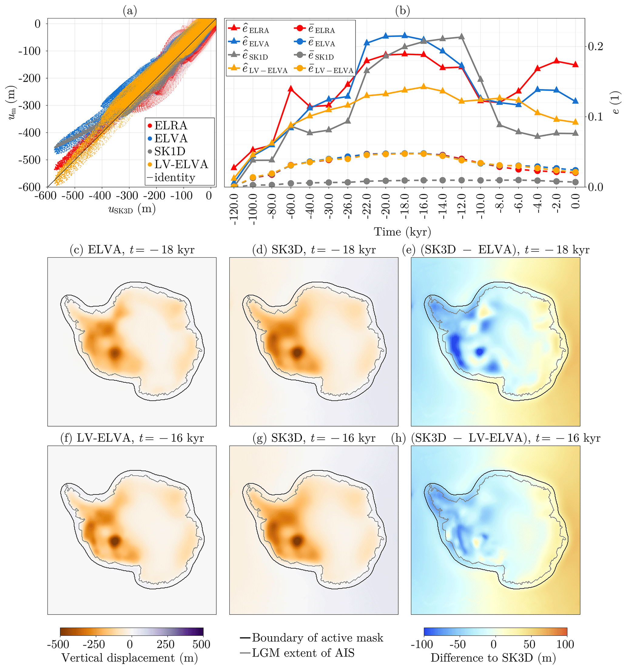
Figure 9 Comparison of Seakon and FastIsostasy, forced by the ice loading from ICE6G_D (Peltier et al., 2018). (a) Displacements at all time steps of ELRA, ELVA, SK1D and LV-ELVA against SK3D for cells within the active mask. (b) Transient mean and maximal displacement errors respectively denoted by $\overline{e}\left(t\right)$ and $\widehat{e}\left(t\right)$ of ELRA, ELVA, SK1D and LV-ELVA with respect to SK3D, for all domain cells. (c–e) Displacement of ELVA, SK3D and their differences for the time step of maximal error. (f–h) Same as (c–e) for LV-ELVA.

The error plot shown in Fig. 9a depicts, for all time steps, the displacement of SK3D, considered to be closest to reality, against ELRA, ELVA, SK1D and LV-ELVA. We hereby only represent the points within the activation mask 𝒜, represented by the black contours of Fig. 9c–h and corresponding to the typical region of interest for ice-sheet modellers. The position around the identity shows that ELVA leads to displacements that are biased towards lower values, especially for $u_{\mathrm{SK}\mathrm{3}\mathrm{D}}\le -\mathrm{300}$ m, where the error comes close to e^abs≃130 m. Although this bias is somewhat smaller for SK1D, it still reaches similar maximal values. In comparison, LV-ELVA is centred around the identity and presents no such bias. This can be explained by the fact that a thinner lithosphere and a less viscous mantle in West Antarctica allows for larger transient displacements around LGM. Furthermore, the spread around the identity, especially around the lower, unbiased displacement values, is an additional metric to take into account. For $u_{\mathrm{SK}\mathrm{3}\mathrm{D}}\ge -\mathrm{300}$ m, SK1D, LV-ELVA and ELVA respectively present the smallest, the intermediate and the largest spread. As expected, ELRA shows a larger bias than LV-ELVA but, surprisingly, a smaller one than SK1D and ELVA. However, the spread of ELRA is larger than for any other model.

Figure 9b depicts the mean and maximal relative difference for ELRA, ELVA, LV-ELVA and SK1D with respect to SK3D. The mean and maximal value respectively relate to the spread around the identity and the bias observed in Fig. 9a. In Fig. 9b, the error metrics are computed for the full domain and therefore include the far field, where the rotational feedback dominates the displacement. Since none of the regional models are capable of capturing this, SK1D shows the smallest mean error over time, with ${\overline{e}}_{\mathrm{SK}\mathrm{1}\mathrm{D}}\left(t\right)<\mathrm{0.01}$. In comparison, ELRA, ELVA and LV-ELVA show larger mean error metrics that are however similar among each other, with $\overline{e}\left(t\right)<\mathrm{0.04}$. When computing the mean error only over the active mask, this difference between SK1D and the regional models vanishes, with $\overline{e}\le \mathrm{0.01}$ for all models. We believe that this latter definition of the mean error is closer than what is relevant to most ice-sheet modellers, but highlighting the larger error in regional models in the far field ensures that the users of FastIsostasy are aware of this limitation. The low values of the mean error that are observed regardless of the model can be explained by the fact that most of the regions, especially the bulk of East Antarctica, can be represented well by intermediate mantle viscosity and lithospheric thickness.

Interestingly, the peak values of ${\widehat{e}}_{\mathrm{SK}\mathrm{1}\mathrm{D}}$ and ${\widehat{e}}_{\mathrm{ELVA}}$ are very close to each other, yielding about 0.22, corresponding to ${\widehat{e}}^{\mathrm{abs}}\simeq \mathrm{130}$ m. In both cases, these values are observed over $t\in [-\mathrm{22},-\mathrm{12}]$ kyr, which corresponds to the 10 kyr of rapid deglaciation following LGM. In comparison, ELRA presents a peak maximal error with a similar timing and a marginally smaller amplitude ${\widehat{e}}_{\mathrm{ELRA}}<\mathrm{0.19}$. However, it presents large errors over the last 6 kyr of simulation. This points out that high errors in ELRA, ELVA and SK1D are to be expected when rapid changes in ice thickness occur – a situation that could be triggered by sustained anthropogenic climate warming. For ELVA, the peak difference to SK3D is observed at $t=-\mathrm{18}$ kyr. The corresponding displacement fields and their difference are plotted in Fig. 9c–e, corroborating that ELVA does not allow for enough displacement in West Antarctica after the LGM. The location of the peak error points out that the use of ELVA, coupled to an ice-sheet model, may lead to significant errors since the WAIS is based on a retrograde bedrock below sea level and is therefore particularly sensitive to the GIA response, as pointed out in the Introduction.

Compared to ELRA, ELVA and SK1D, LV-ELVA reduces the maximal error down to about ${\widehat{e}}_{\mathrm{LV}-\mathrm{ELVA}}\le \mathrm{0.14}$, which corresponds to ${\widehat{e}}^{\mathrm{abs}}\le \mathrm{80}$ m. The displacement fields for the time $t=-\mathrm{14}$ kyr are plotted in Fig. 9f–h and show that the near-field displacement is reasonably well matched, even for the time step showing the largest error metrics. In particular, the displacement is slightly underestimated in most of the active mask. Since this appears to be a systematic offset, it could easily be corrected by tuning the density and/or the viscosity chosen for LV-ELVA.⁸ We however decide not to do so to highlight the differences to SK3D without additional tuning.

Throughout Test 4, SK3D has been used as the baseline model. In Sect. D, we show a similar analysis that compares ELRA and ELVA by using SK1D as a baseline. There it appears (1) that ELVA presents smaller errors than ELRA and (2) that LV-ELVA presents smaller errors compared to SK3D than ELVA compared to SK1D.

Runtime analysis. Despite the errors compared to Seakon and potentially to any 3D GIA model, we believe that FastIsostasy can be a particularly appealing tool, since the 122 kyr run takes only about 9 min to compute for a horizontal resolution of h=20 km, resulting in 350×350 grid points. For ELVA, the absence of LV leads to a reduced computation time of only about 4 min and outperforms ELRA, which requires about 6 min. These computations were performed on an NVIDIA GeForce RTX 2070, a low-cost GPU with moderate performance by the standards of 2024. Although the time stepping is adaptive, no values beyond dt=10 years are used. This potentially provides the ice-sheet model with an input that is very dense in time, for instance as opposed to Gomez et al. (2018).

In comparison, the Seakon simulation takes about 4.5 d on 150 CPUs with a time step of $dt\in [\mathrm{125},\mathrm{1000}]$ years. Assuming an ideal parallelisation scaling of 100 %, this corresponds to about 1×10⁶ min of CPU runtime, which roughly corresponds to 5 orders of magnitude more than what FastIsostasy requires. The models used in Albrecht et al. (2023) and Zhong et al. (2022) present smaller computation times, reducing this down to 4 orders of magnitude.

Furthermore, the power consumption of the GPU used in the present study is 185 W,⁹ compared to a typical value of more than 100 W for a single, modern CPU. As the energy consumption is expressed as the product of power and computation time, FastIsostasy appears to be less energy-consuming than Seakon by several orders of magnitude. Finally, we draw attention to the fact that the acquisition price of the GPU used here is a few hundred euros, which is far less than that of a large CPU cluster.

Of course, the runtime of Seakon and FastIsostasy are not directly comparable: Seakon solves the global GIA problem, which requires a grid with many more degrees of freedom that reaches down to the core–mantle boundary. The output of Seakon is much richer, since it includes, among others, the rotational feedback, the position of migrating shorelines, the horizontal displacement of the bedrock and the relative sea level at any point on Earth. Nonetheless, these quantities tend to be less relevant for stand-alone ice-sheet modelling, and FastIsostasy therefore offers an opportunity to regionally mimic the behaviour of a 3D GIA model at very low computational, energy and financial cost.

5 Conclusions

Throughout all the tests, FastIsostasy displays a maximal and mean error over space of $\widehat{e}\left(t\right)<\mathrm{0.2}$ and $\overline{e}\left(t\right)<\mathrm{0.05}$, both being typically much smaller for most time steps. In particular, Test 1 has shown that the discretisation error of FastIsostasy is very small and that, with an increasing problem size, its computational expense scales better than what is typically obtained with FDM, FVM and FEM solvers. Test 2 has shown that FastIsostasy represents the deformational response and the SSH perturbation with a relatively low error compared to 1D GIA models, despite solving the problem on a 2D regional grid. Test 3 and Test 4 have shown that LV-ELVA produces greatly reduced errors with respect to SK3D, compared to ELRA and ELVA and even to SK1D for the near-field GIA response. This means that the model uncertainty between FastIsostasy and Seakon is smaller than the upper bound on parametric uncertainty, given by the difference between a 1D and a 3D Earth structure (Albrecht et al., 2023).

In conclusion, FastIsostasy can greatly reduce the transient error in bedrock displacement compared to ELRA and ELVA and even to 1D GIA models for regions of significant LV. This was achieved by introducing LV-ELVA, which generalises the work of Bueler et al. (2007) and Coulon et al. (2021) and was coupled to ReSeLeM, which regionally approximates the transient changes in ocean load. Whereas the differences between FastIsostasy and global GIA models are within the range of parametric uncertainties, the computation time is typically reduced by 3 to 5 orders of magnitude. For most ice-sheet models, FastIsostasy can thus represent a leap in GIA comprehensiveness at very low computational cost, even for high-resolution runs on the timescale of glacial cycles. This has straightforward applications, since the GIA response is particularly relevant for the many marine-based regions of the AIS, where significant LV of the solid Earth can be present. This is the case for the Amundsen sector, which could become the largest source of sea-level rise in the coming century and therefore requires projections that account, as accurately as possible, for the stabilising effect of GIA.

Since fields of the lithospheric thickness and the upper-mantle viscosity can be easily found in the literature, FastIsostasy reduces the difficulty of creating meaningful ensembles compared to relaxed rheologies (Coulon et al., 2021). The very short runtime of FastIsostasy offers an efficient method of propagating the uncertainties of the solid-Earth parameters to past and future climatic scenarios.

We believe that GIA modellers, as well as the few ice-sheet models that are coupled to a 3D GIA model, can benefit from FastIsostasy, since it can be used as a fast-prototyping tool. In particular, a scheme to tune the parameters of FastIsostasy can turn it into an emulator of a 3D GIA model with better interpretability than, for instance, machine learning techniques. Nonetheless, it should be emphasised that some scientific questions can only be answered with a global 3D GIA model and that FastIsostasy is a complementary tool that does not aim to replace it. Finally, we believe that the relatively abbreviated code of FastIsostasy and its few equations compared to 1D or 3D GIA models are particularly well suited for educational purposes.

Appendix A: From ELRA to LV-ELVA

Following Le Meur and Huybrechts (1996), the governing equations of ELRA yield

$$\begin{array}{}\text{(A1)}& {\displaystyle }{\mathit{\rho }}^{\mathrm{m}}g{u}^{\mathrm{eq}}+D{\mathrm{\nabla }}^{\mathrm{4}}{u}^{\mathrm{eq}}={\mathit{\sigma }}^{zz},\text{(A2)}& {\displaystyle \frac{\partial u}{\partial t}}={\displaystyle \frac{\mathrm{1}}{\mathit{\tau }}}(u-u^{\mathrm{eq}}),\end{array}$$

with u^eq as the equilibrium displacement and all further quantities already introduced in this paper. Equation (A1) can be solved by convolving the load with a Green's function derived from a Kelvin function of order 0, as described in Le Meur and Huybrechts (1996). In FastIsostasy, the convolution is performed via FFTs, which is much faster than a computation in a time domain. Coulon et al. (2021) generalised the equations of ELRA to a laterally variable lithospheric thickness and relaxation time (LV-ELRA):

$$\begin{array}{}\text{(A3)}& {\displaystyle }{\mathit{\rho }}^{\mathrm{m}}g{u}^{\mathrm{eq}}+{\displaystyle \frac{{\partial }^{\mathrm{2}}{M}_{xx}^{\mathrm{eq}}}{\partial x^{\mathrm{2}}}}+\mathrm{2}{\displaystyle \frac{{\partial }^{\mathrm{2}}{M}_{xy}^{\mathrm{eq}}}{\partial x\partial y}}+{\displaystyle \frac{{\partial }^{\mathrm{2}}{M}_{yy}^{\mathrm{eq}}}{\partial y^{\mathrm{2}}}}={\mathit{\sigma }}^{zz},\text{(A4)}& {\displaystyle \frac{\partial u}{\partial t}}={\displaystyle \frac{\mathrm{1}}{\mathit{\tau }(x,y)}}(u-u^{\mathrm{eq}}),\end{array}$$

with $M_{xx}^{\mathrm{eq}}$, $M_{xy}^{\mathrm{eq}}$ and $M_{yy}^{\mathrm{eq}}$ as the flexural moments at equilibrium, computed by introducing u^eq into Eqs. (10)–(12). For ELRA as well as LV-ELRA, a relaxed rheology is used, which presents the limitations explained in Sect. 1.3. ELVA, as proposed by Bueler et al. (2007), Cathles (1975), and Lingle and Clark (1985), addresses this limitation because its governing equation is directly parameterised by viscosity:

$$\begin{array}{}\text{(A5)}& \mathrm{2}\mathit{\eta }\left|\mathrm{\nabla }\right|{\displaystyle \frac{\partial u}{\partial t}}+{\mathit{\rho }}^{\mathrm{m}}g{u}^{\mathrm{eq}}+D{\mathrm{\nabla }}^{\mathrm{4}}u={\mathit{\sigma }}^{zz}.\end{array}$$

However, this assumes a constant lithospheric thickness $T(x,y)=T$ and sub-lithospheric mantle viscosity $\mathit{\eta }(x,y)=\mathit{\eta }$ throughout the domain, which therefore prevents the representation of LV. We tried to generalise the derivation presented in Cathles (1975) to LV; however this was unsuccessful. Instead, we combined Eqs. (A3) and (A5), thus obtaining

$$\begin{array}{}\text{(A6)}& \begin{array}{rl}& \mathrm{2}\mathit{\eta }(x,y)\left|\mathrm{\nabla }\right|{\displaystyle \frac{\partial u}{\partial t}}+{\mathit{\rho }}^{\mathrm{m}}g{u}^{\mathrm{eq}}+{\displaystyle \frac{{\partial }^{\mathrm{2}}{M}_{xx}}{\partial x^{\mathrm{2}}}}+\mathrm{2}{\displaystyle \frac{{\partial }^{\mathrm{2}}{M}_{xy}}{\partial x\partial y}}+\\ & {\displaystyle \frac{{\partial }^{\mathrm{2}}{M}_{yy}}{\partial y^{\mathrm{2}}}}={\mathit{\sigma }}^{zz},\end{array}\end{array}$$

with the flexural moments accounting for the laterally variable lithospheric thickness. By introducing a pressure term, as done in Eq. (8), and accounting for the distortion K, we obtain the governing equation of LV-ELVA, as written in Eq. (9). For constant parameters, LV-ELVA simplifies to the equation of ELVA and can be therefore understood as an ad hoc generalisation that reduces the error made compared to a 3D GIA model. Using ELVA in FastIsostasy is simply achieved by running LV-ELVA with constant parameters. This seamless approach offers a code that is easier to maintain and an interface that is simpler to use, at the expense of a minor increase in computational expense compared to the use of a specific solver that takes advantage of the simplifications made in ELVA.

Appendix B: Ocean surface function

The function $\stackrel{\mathrm{̃}}{A}\left(\mathrm{s}\right):\mathbb{R}\to \mathbb{R}$ is here computed by summing the surfaces of cells situated below the BSL s, based on the 1 arcmin global topography of ETOPO1 (Amante and Eakins, 2009). Note that this slightly overestimates the ocean surface, since all regions below sea level are counted as part of the ocean, including, for instance, parts of the Netherlands. To tackle this, we introduce a bias correction scaling γ, which avoids any offset for the present-day value A_pd and depends on the uncorrected value $\stackrel{\mathrm{̃}}{A}\left(s\right)$:

$$\begin{array}{}\text{(B1)}& A\left(s\right)=\mathit{\gamma }\stackrel{\mathrm{̃}}{A}\left(s\right),\mathrm{with}\mathit{\gamma }={\displaystyle \frac{A_{\mathrm{pd}}}{\stackrel{\mathrm{̃}}{A}(s=\mathrm{0})}}.\end{array}$$

To reduce the runtime, we precompute A(s) as a piecewise linear interpolator for $s\in [-\mathrm{150},\mathrm{70}]$ years with a discretisation of Δs=0.1 m. The resulting function is depicted in Fig. 4c and shows that, for the range of realistic sea-level contributions over glacial cycles, the trapezoidal approximation leads to variations of the ocean surface between −7 % and +4 % around the present-day value.

Appendix C: Scaling the effective viscosity

Two important characteristics of the mantle have to be accounted for such that the Maxwell time $\mathit{\tau }=\mathit{\eta }{E}^{-\mathrm{1}}$ of FastIsostasy is comparable to that of a 3D GIA model. This is done by introducing two correction factors. First, one of the underlying assumptions made by Cathles (1975) is that the mantle is incompressible; i.e. νⁱ=0.5 is assumed as opposed to ν₀=0.28 for the elastic lithosphere. In reality, the mantle is however a compressible medium with ν^c≃0.28. We now look for ηⁱ, the viscosity that has to be used in the incompressible case in order to match the Maxwell time of the compressible case. By introducing the shear modulus $G=E\left(\mathrm{2}\right(\mathrm{1}+\mathit{\nu }){)}^{-\mathrm{1}}$, we obtain

$$\begin{array}{}\text{(C1)}& {\displaystyle \frac{{\mathit{\eta }}^{\mathrm{i}}}{\mathrm{2}G(\mathrm{1}+{\mathit{\nu }}^{\mathrm{i}})}}={\displaystyle \frac{{\mathit{\eta }}^{\mathrm{c}}}{\mathrm{2}G(\mathrm{1}+{\mathit{\nu }}^{\mathrm{c}})}},\text{(C2)}& {\displaystyle }\iff {\mathit{\eta }}^{\mathrm{i}}={\displaystyle \frac{\mathrm{1}+{\mathit{\nu }}^{\mathrm{i}}}{\mathrm{1}+{\mathit{\nu }}^{\mathrm{c}}}}{\mathit{\eta }}^{\mathrm{c}}={\mathit{\alpha }}^{\mathrm{c}}{\mathit{\eta }}^{\mathrm{c}}.\end{array}$$

In essence, this means that compressible media have a larger Maxwell time and that we need to slightly increase the viscosity values to render this, since Eq. (A5) is used to postulate Eq. (9) and assumes an incompressible viscous flow. This is supported by Fig. C1, which shows that a 1D GIA model displays longer decay times for a compressible mantle, compared to an incompressible one.

Second, both the shear modulus and the viscosity depend on the temperature of the medium. For instance, a positive temperature anomaly in the mantle leads to a negative anomaly of both viscosity and shear modulus. This means that the decrease in the Maxwell time due to the decrease in viscosity is somewhat compensated by the decrease in the shear modulus. We have chosen to compute this scaling by calibrating FastIsostasy to results of a 3D GIA model:

$$\begin{array}{}\text{(C3)}& \mathit{\eta }=\exp \left({\log }_{\mathrm{10}}\left({\displaystyle \frac{{\mathit{\eta }}_{\mathrm{0}}}{{\mathit{\eta }}^{\mathrm{i}}}}\right)\right){\mathit{\eta }}^{\mathrm{i}}={\mathit{\alpha }}^{\mathrm{G}}\left({\mathit{\eta }}^{\mathrm{i}}\right)\cdot {\mathit{\eta }}^{\mathrm{i}},\end{array}$$

with η₀=10²¹ Pa s the calibration constant used throughout this work. We thus obtain a relation between the viscosity η^c, inferred from seismic measurements, and the corrected effective viscosity η, ultimately used in FastIsostasy:

$$\begin{array}{}\text{(C4)}& \mathit{\eta }={\mathit{\alpha }}^{\mathrm{G}}{\mathit{\alpha }}^{\mathrm{c}}{\mathit{\eta }}^{\mathrm{c}}=\mathit{\alpha }{\mathit{\eta }}^{\mathrm{c}}.\end{array}$$

If the depth dimension is lumped according to Eq. (B1), then the viscosity field ${\mathit{\eta }}_{\mathrm{1}}^{\mathrm{eff}}$, representing the compound of layers from l=1 to l=L, is used for η^c.

Figure C1 Decay times of a 1D GIA model with ν^c=0.28 (compressible) and νⁱ=0.5 (incompressible).

Appendix D: Complementary information on Test 3 and Test 4

The anomalies of lithospheric thickness and upper-mantle viscosity used in Test 3 are represented in Fig. D1 and result from a scaled Gaussian distribution 𝒩(0,σ) with $\mathit{\sigma }=(W/\mathrm{4}{)}^{\mathrm{2}}\mathit{I}$ and $\mathit{I}\in {\mathbb{R}}^{\mathrm{2}\times \mathrm{2}}$ as the identity matrix.

In addition to Test 3, we perform two simulations with laterally constant Earth structures in Seakon. The first one corresponds to PREM (Dziewonski and Anderson, 1981), and the second corresponds to a single-layer mantle without an elastic lithosphere. The results are respectively depicted in Fig. D2a and b. Unsurprisingly, the first case shows a very similar error pattern to what is obtained in Test 2 and highlights that the main error source for FastIsostasy comes from the lumped depth dimension rather than from the generalisation of ELVA to LV-ELVA. The second case shows that, in the absence of a lithosphere, the match between Seakon and FastIsostasy yields $\overline{e}\left(t\right)<\mathrm{0.04}$ and $\widehat{e}\left(t\right)<\mathrm{0.08}$. In particular, this example shows that, in both models, the absence of a lithosphere effectively decouples neighbouring cells due to the absence of flexural moments.

Whereas Fig. 9 uses SK3D as a baseline for the error metrics, we propose using SK1D as a baseline to compare ELRA and ELVA in Fig. D3. In Fig. D3, it appears that ELRA is more biased towards large displacements than ELVA. Furthermore, the mean error is similar for both models, but the maximal error is higher overall for ELRA, with $\widehat{e}\left(t\right)<\mathrm{0.21}$. In comparison, the maximum error in ELVA yields $\widehat{e}\left(t\right)<\mathrm{0.16}$. The middle row of Fig. D3 highlights that the higher error in ELRA stems from an overestimated displacement in Marie Byrd Land. In comparison, the bottom row shows that ELVA displays a much more homogeneously distributed error.

Figure D1 Gaussian-shaped LV used in Test 3 for (a) a lithospheric thinning, (b) a lithospheric thickening, (c) a viscosity decrease and (d) a viscosity increase towards the centre of the domain.

Figure D2 Comparison of FastIsostasy and Seakon for (a) a layered mantle following PREM and (b) a mantle with a single layer and no lithosphere.

Table D1 Runtime of FastIsostasy in Test 3 for a resolution of $N_x=N_y=\mathrm{128}$, on a single CPU (Intel i7-10750H, 2.60 GHz).

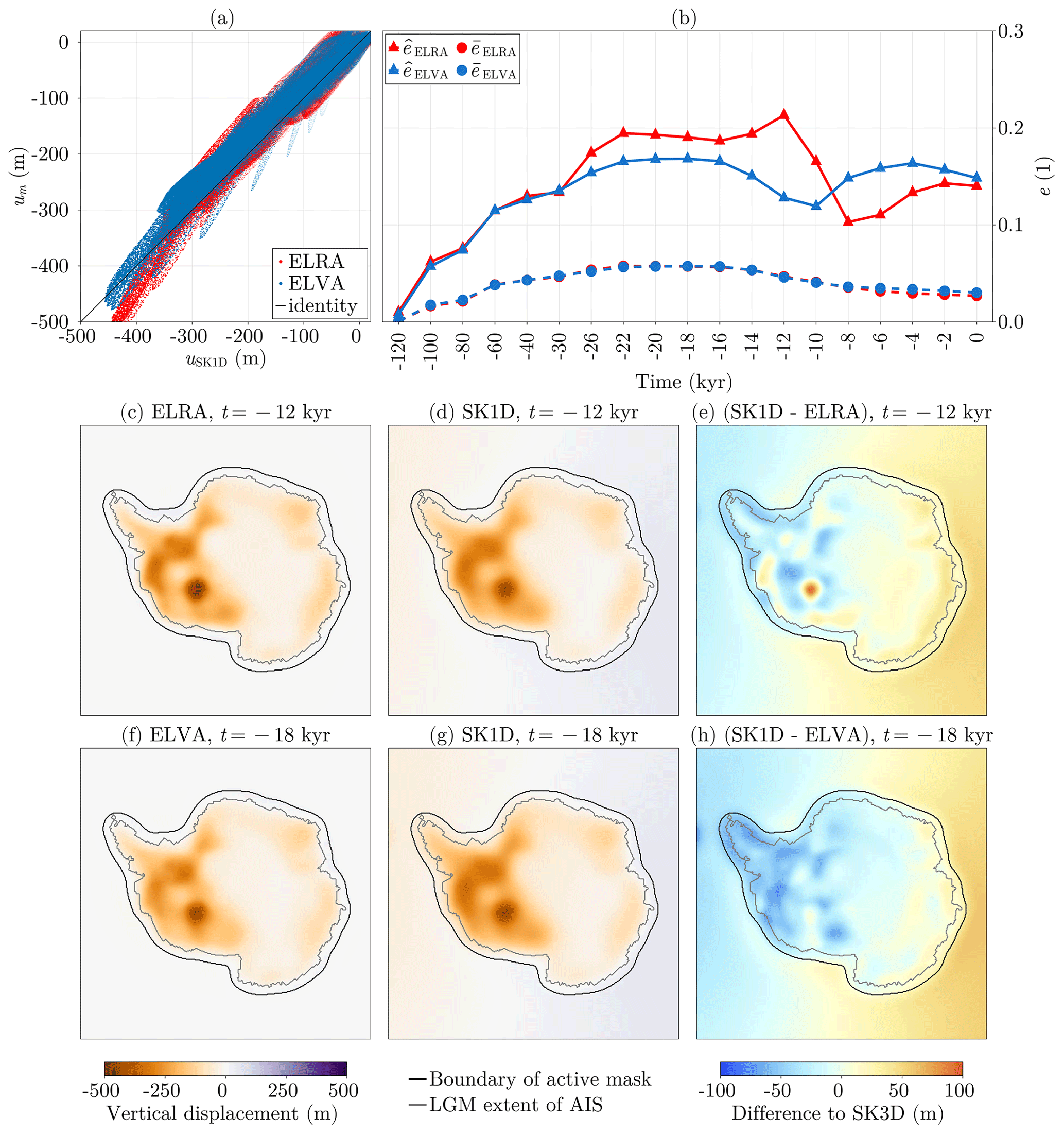
Figure D3 Comparison of ELRA, ELVA and SK1D forced by ICE6G_D (Peltier et al., 2018). (a) Displacements at all time steps of ELRA and ELVA against SK1D, for cells within the active mask. (b) Transient mean and maximal errors in ELRA and ELVA with respect to SK1D. (c–e) Displacement of ELRA, SK1D and their differences for the time step of maximal error. (f–h) Same as (c–e) for ELVA.