the Creative Commons Attribution 4.0 License.
the Creative Commons Attribution 4.0 License.
 | 27 Jun 2024
A computationally efficient parameterization of aerosol, cloud and precipitation pH for application at global and regional scale (EQSAM4Clim-v12)
Samuel Rémy
Jason E. Williams
Vincent Huijnen
Johannes Flemming
The Equilibrium Simplified Aerosol Model for Climate version 12 (EQSAM4Clim-v12) has recently been revised to provide an accurate and efficient method for calculating the acidity of atmospheric particles. EQSAM4Clim is based on an analytical concept that is not only sufficiently fast for chemical weather prediction applications but also free of numerical noise, which also makes it attractive for air quality forecasting. EQSAM4Clim allows the calculation of aerosol composition based on the gas–liquid–solid and the reduced gas–liquid partitioning with the associated water uptake for both cases and can therefore provide important information about the acidity of the aerosols. Here we provide a comprehensive description of the recent changes made to the aerosol acidity parameterization (referred to as a version 12) which builds on the original EQSAM4Clim. We evaluate the pH improvements using a detailed box model and compare them against previous model calculations and both ground-based and aircraft observations from the USA and China, covering different seasons and scenarios. We show that, in most cases, the simulated pH is within reasonable agreement with the reference results of the Extended Aerosol Inorganics Model (E-AIM) and of satisfactory accuracy.
- Article
(8617 KB) - Full-text XML
- Companion paper 2
- Companion paper 3
-
Supplement
(789 KB) - BibTeX
- EndNote


In order to address the relevance of gas–aerosol partitioning and aerosol water for climate and air quality studies, EQSAM was developed as a compromise between numerical speed and accuracy (Metzger et al., 2002). EQSAM has been widely used in many air quality and climate modeling systems worldwide (Metzger et al., 2018), including ECMWF's Integrated Forecasting System (IFS) (Flemming et al., 2015) and the OpenIFS (Huijnen et al., 2022). Recently, the EQSAM version for Climate Applications (EQSAM4Clim) (Metzger et al., 2016b) has been implemented in the IFS, with extensions to represent aerosols, trace gases and greenhouses gases, called “IFS-COMPO” (also previously known as “C-IFS”, Flemming et al., 2015); see the accompanying paper (Rémy et al., 2024). In contrast to EQSAM, EQSAM4Clim is entirely based on a compound-specific single-solute coefficient (νi), which was introduced in Metzger et al. (2012) to accurately parameterize the single solution hygroscopic growth, considering the Kelvin effect. This νi approach accounts for the water uptake of concentrated nanometer-sized particles up to dilute solutions, i.e., from the compounds relative humidity of deliquescence (RHD) up to supersaturation (Köhler theory). EQSAM4Clim extends the νi approach to multicomponent mixtures, including semi-volatile ammonium compounds and major crustal elements. The advantage of EQSAM4Clim is that the entire gas–liquid–solid aerosol phase partitioning and water uptake, including major mineral cations, is solved analytically without iterations and is thus computationally very efficient. This makes EQSAM4Clim not only suited for climate simulations but also applicable to air quality applications at the regional and global scale and ideal for high-resolution numerical weather prediction (NWP) coupled with comprehensive atmospheric chemistry providing global values of particulate matter, as done in the Copernicus Atmosphere Monitoring Service (CAMS; Peuch et al., 2022; Rémy et al., 2022) for example, using IFS.
Previously, the use of EQSAM4Clim has undergone a rigorous assessment across different timescales, through a comparison with various observations and reference simulations on climate timescales using more than a decade of independent observations (e.g., Metzger et al., 2018). Moreover, a comparison of simulated aerosol optical depth (AOD) has been made against various satellite data at NWP timescales to validate the Polar Multi-sensor Aerosol properties (PMAp) AOD product version 2 AOD at a 1-hourly time resolution (Metzger et al., 2016a). EQSAM4Clim has also been used as part of air quality assessments through, e.g., the 2019 European Monitoring and Evaluation Programme (EMEP) report on transboundary particulate matter, photo-oxidants, and acidifying and eutrophying components (Fagerli et al., 2019), and evaluated in the air quality modeling system CAMx over the continental USA with 12 km grid resolution for winter and summer months. It was found that EQSAM4Clim accurately parameterizes the gas–liquid–solid aerosol partitioning and associated aerosol water uptake sufficiently fast and free of numerical noise (Koo et al., 2020), which is true at all timescales. This is due to its unique analytical structure, which also makes it particularly attractive for air quality assessments such as those provided by CAMS. Most recently, the latest version of EQSAM4Clim has been implemented in IFS-COMPO as presented in Metzger et al. (2022) and Metzger et al. (2023). A more comprehensive evaluation of the performance on global pH values and resulting effects on particulate matter in IFS-COMPO is presented in the accompanying study of Rémy et al. (2024).
This technical note provides a description of the improved aerosol acidity parameterization applied in EQSAM4Clim-v12. We show an extensive validation against reference model calculations using E-AIM as described in Wexler and Clegg (2002) and Friese and Ebel (2010), using the detailed case study on aerosol acidity provided by Pye et al. (2020).
The overall gas–liquid–solid partitioning and aerosol water uptake parameterization are the same as described and evaluated in Metzger et al. (2012) and Metzger et al. (2016b), with further evaluation being provided in Metzger et al. (2018). Here we limit the description to those new features added to previous versions.
2.1 General features
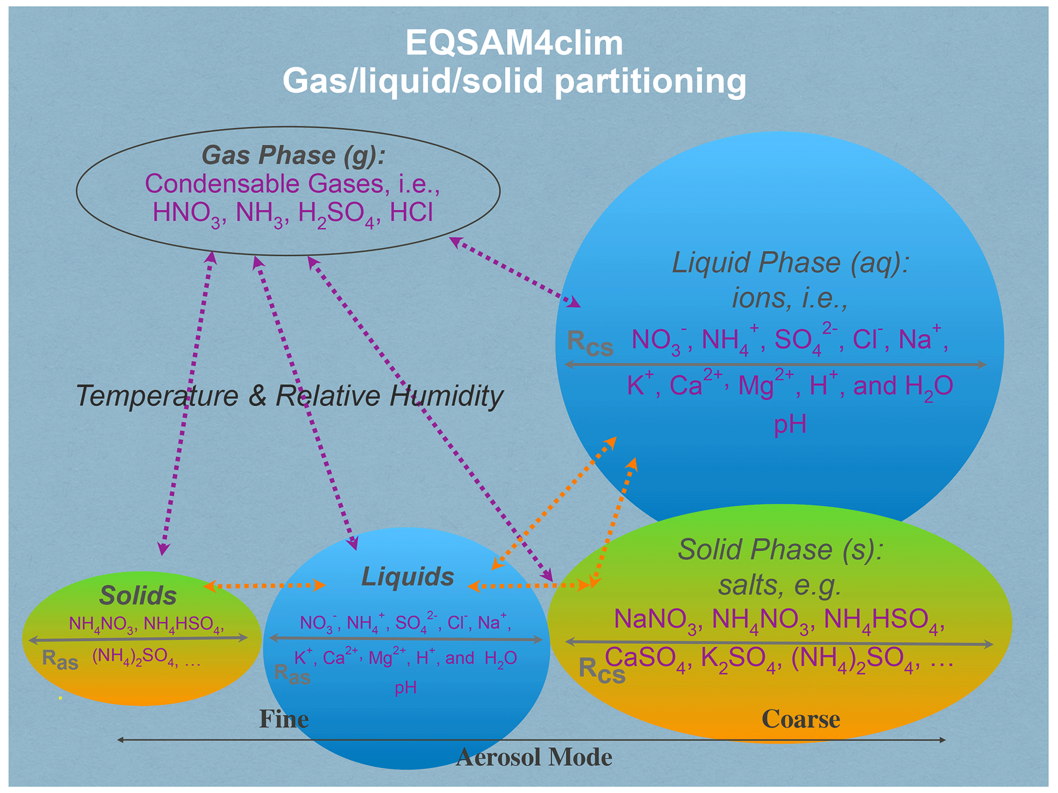
A schematic of the various input parameters needed for use in EQSAM4Clim is shown in Fig. 1, where chemical species from each phase type is given. EQSAM4Clim is based on a compound-specific single-solute coefficient (νi), which was introduced in Metzger et al. (2012) for single solute solutions and extended to multi-component mixtures by Metzger et al. (2016b) to include semi-volatile ammonium (NH4+) compounds and major crustal elements. A feature of the νi approach is that the entire gas–liquid–solid aerosol phase partitioning and water uptake can be solved analytically without iterations and hence without numerical noise.
As input, EQSAM4Clim takes (i) the meteorological parameters air temperature (T) and relative humidity (RH); (ii) the aerosol precursor gases, i.e., major oxidation products of emissions from natural sources and anthropogenic air pollution represented by ammonia (NH3), hydrochloric acid (HCl), nitric acid (HNO3) and sulfuric acid (H2SO4); and (iii) the ionic aerosol concentrations, i.e., lumped (both liquid and solid) anions, sulfate (), bisulfate (), nitrate (NO3−), chloride (Cl−) and lumped (liquid + solid) cations, i.e., NH4+, sodium (Na+), potassium (K+), magnesium (Mg2+) and calcium (Ca2+).
The equilibrium aerosol composition and aerosol associated water mass (AW) are calculated by EQSAM4Clim through the neutralization of anions by cations, which yields numerous salt compounds, i.e., the sodium salts Na2SO4, NaHSO4, NaNO3 and NaCl; the potassium salts K2SO4, KHSO4, KNO3 and KCl; the ammonium salts (NH4)2SO4, NH4HSO4, NH4NO3 and NH4Cl; the magnesium salts MgSO4, Mg(NO3)2 and MgCl2; and the calcium salts CaSO4, Ca(NO3)2 and CaCl2. All salt compounds (except CaSO4) can partition between the liquid and solid aerosol phase, depending on T, RH, AW and the temperature-dependent relative humidities of deliquescence of (a) single solute compound solutions (RHD) and (b) mixed salt solutions (Metzger et al., 2016b).
Based on the RHD of the single solutes, the (mixed) solution liquid–solid partitioning is calculated, whereby all compounds for which the RH is below the RHD are assumed to be precipitated, such that a solid and liquid phase can coexist. The liquid–solid partitioning is strongly influenced by mineral cations and in turn largely determines the aerosol pH (Sect. 3).
EQSAM4Clim estimates the concentration of the hydronium ion (H+) [mol m−3 (air)] and, subsequently, the pH of the solution from electroneutrality (Z0 [mol m−3 (air)]) after neutralization of all anions by all cations in the system (following the neutralization reaction order given by Table 3 of Metzger et al., 2016b), using the effective hydrogen concentrations H+,* and Z* that are derived from Eqs. (1)–(8).
Note that the auto-dissociation of H2O is taken into account, but currently no dissolution–dissociation of aerosol precursor gases such as sulfur dioxide (SO2), nitric acid (HNO3), hydrogen chloride (HCl) or ammonia (NH3) is taken into account, as this is typically considered in the aqueous-phase chemistry module of any global chemistry forecast model. The initial H+,0 concentration [mol m−3 (air)] after cation–anion neutralization is obtained from
with tAnions and tCations (hereafter referred to as tCAT) representing the total absolute charge number density of all anions and cations [mol m−3 (air)], respectively, that are present in the given aerosol composition. The concentration is denoted by square brackets, while Z− and Z+ denote the charge of tAnions and tCations, respectively, and [H+,0] denotes the initial hydronium ion concentration per volume air and which also depends on the auto-dissociation of water Kw [mol2 kg−2 (H2O)]. This is derived from Eq. (3) considering the temperature dependency as widely assumed in equilibrium models.
with T0=298 K.
2.2 Updates to the acidity component
2.2.1 Dependency of H+ on the chemical domain
The neutralization equation does not correct for non-ideal solutions, such as described in Pye et al. (2020) and the references therein. For that purpose, with v12, for EQSAM4Clim we introduce a new factor FN, which depends on the degree of neutralization of the given aerosol composition and is used here to correct the initial [H+,0] (Eq. 2). FN is obtained from
with X denoting the sum of all anions noted above, while Y=tNH4, i.e., the sum of NH3 and . FN is applied without further scaling factors for ranges of FN<0.9 with ambient temperatures below 293 K.
Table 1H+ correction factors introduced with EQSAM4Clim-v12 for the chemical domains introduced in Metzger et al. (2016b).
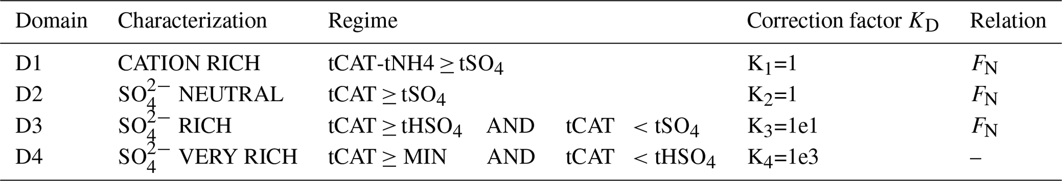
For cases outside this range (FN≥0.9 or T≥293 K), FN needs to be scaled by 10 and multiplied by the factor KD given in Table 1, in order to account for chemical processes which are not resolved by the parameterizations (particularly concerning and free H2SO4). Following Table 2 of Metzger et al. (2016b), four chemical domains are considered to correct [H+,0] obtained with Eq. (2). No additional correction () is needed for the neutral cases (D1–D2), i.e., where cations are in excess of total , thus preventing the formation of all salts (see Table 1 of Metzger et al., 2016b). For the case rich in (D3), FN and KD from Table 1 are multiplied, while for the case very rich in (D4), only a constant correction factor (KD) is applied to correct Eq. (2). In Table 1, tCAT denotes the sum of cations given in Eq. (2), and tSO4 is the sum of all including and H2SO4, while tHSO4 denotes the sum of and H2SO4.
Additionally, we consider three cases for estimating the H+ concentration, according to the possible solutions of Eq. (1), i.e.,
with LWCtot being the total liquid water content [kg(H2O) m−3 (air)] as defined below in Eqs. (9a)–(9d). LWCo=1 [kg m−3 (air)] and [mol kg−1 (H2O), a reference solution and reference molality, respectively, to match units (Metzger et al., 2012, 2016b; Pye et al., 2020). Z* is given by Eq. (6) and denotes the sum of our initial hydrogen concentration [H] and [H], an effective hydrogen concentration in a neutral solution (pH =7), which is given by Eq. (7) but empirically derived for our parameterization:
with Kw from Eq. (3); a constant [–]; and the molar mass of water, mw [kg mol−1]. RH denotes the fractional relative humidity [0–1].
Finally, the H+ concentration of a given solution is obtained from
2.2.2 Dependency of pH on the liquid water content
For EQSAM4Clim-v12, five different pH values can be computed from the revised H+ [mol m−3 (air)] computation (Sect. 2.2.1) for diagnostic output. Therefore, EQSAM4Clim-v12 allows the differentiation of the various LWC [kg(H2O) m−3 (air)] values associated with different types of atmospheric aerosols, haze/fog, or cloud droplets contained in the troposphere as defined in Eqs. (9a)–(9e):
Here, (i) LWCequil [kg(H2O) m−3 (air)] denotes the equilibrium water content calculated within EQSAM4Clim (from Eq. 22 in Metzger et al., 2016b), (ii) LWCnoneq is the aerosol liquid water content associated with aerosol species not considered in the equilibrium computations of EQSAM4Clim (e.g., from chemical aging of pre-existing organic or black carbon particles as used, e.g., in Metzger et al., 2016a, and Metzger et al., 2018), (iii) LWCcloud denotes the cloud liquid water content, (iv) LWCprecip denotes the liquid water content of a given precipitation flux,and finally (v) LWCtotal denotes the sum of LWC of Eqs. (9a)–(9d). The pH values of Eqs. (9b)–(9e) are an optional output feature and require the corresponding input to EQSAM4Clim-v12 (e.g., in any 3-D application these are provided by the forecasting model). It is important to note that all pH and H+ values are only for diagnostic output, as these values are not used within EQSAM4Clim.
In contrast to other aerosol equilibrium models such as E-AIM, EQSAM4Clim has a fully analytical structure which does not depend on the pH. However, accounting for the different pH values is important for air quality and climate applications because of the influence of solution pH on aqueous-phase chemistry in terms of production and the subsequent deposition processes. The pH of aerosols controls their impact on climate and human health. Also note that in the case where an accurate pH calculation is needed, reference calculations from E-AIM should be considered instead, as it has been successfully applied to a wide range of applications. E-AIM is, however, not available nor suitable for 3D applications. With EQSAM4Clim-v12 we try to find a compromise between computational speed and accuracy, so the pH parameterization might not always be applicable, although we show EQSAM4Clim-v12 performs well over a wide range of atmospheric conditions (see Sect. 3 and the accompanying study of Rémy et al., 2024).
In this section, we present comparisons of the revised pH parameterization of EQSAM4Clim-v12 against a wide range of data from different measurement sites and field campaigns spanning different locations for different years, which also was used in the comprehensive pH review study of Pye et al. (2020). In Pye et al. (2020) five distinct cases were defined and used to evaluate the simulated pH of various thermodynamic models, including E-AIM. We therefore select the same observational data for input to the box model calculations and also use the E-AIM model output as a reference to evaluate the revised pH parameterization. It should be noted that E-AIM is much too computationally expensive to be applied in a large-scale atmospheric model. Details of the five cases used are provided below (see also Table 5 of Pye et al., 2020, and the references therein), i.e., here sorted by decreasing complexity of the chemical system with respect to the aerosol composition.
-
Europe. Cabauw Experimental Site for Atmospheric Research (CESAR), NL (51.970° N, 4.926° E), 2 May 2012–4 June 2013, N=2646: Mg2+, Ca2+, K+, Na+, HCl + Cl−, NH3 + , HNO3 + , H2SO4 + + , H2O.
-
Asia. Measurement site Tianjin, CN (39.7° N, 117.1° E), 9–22 August 2015, N=241: Mg2+, Ca2+, K+, Na+, HCl + Cl−, NH3 + , HNO3 + , H2SO4 + + , H2O.
-
SE USA. Southern Oxidant and Aerosol Study (SOAS) campaign, Centreville (32.9° N, 87.1° W), USA, 6 June–14 July 2013,
N=787 (no mineral cations): Na+, , , , , H2O -
SW USA. California Nexus (CalNex) campaign, Pasadena (34.15° N, 118.1° W), CA, USA, 17 May–15 June 2010, N=493 (no mineral cations and no sodium): , , , , H2O.
-
NE USA aloft. Wintertime Investigation of Transport, Emissions, and Reactivity (WINTER) campaign, 3 February 2015, N=3613 (no mineral cations, no sodium): , , , , H2O.
A total of more than 7700 data points are available for evaluation from these campaigns covering a wide range of RH (between 20 %–90 % RH) and T (≈250 to 310 K). Moreover, relevant input is provided for assessing the performance over a complete year (Cabauw), summertime (e.g., SOAS) and wintertime (WINTER). Note that only the correction factors needed for the revised H+ computations (shown in Table 1) have been iteratively derived by comparing the diagnostic pH output of EQSAM4Clim-v12 with the reference pH computations of E-AIM for these five cases (using error minimizing on the log-scale), while the water uptake calculation is identical to that described in Metzger et al. (2016b).
3.1 Aerosol pH
To evaluate the revised pH parameterization of EQSAM4Clim-v12, we compare the resulting values against the output of the E-AIM reference model for the five field campaign cases. In Fig. 2 the results of EQSAM4Clim-v12 and E-AIM are shown and compared to measurements at the Cabauw Experimental Site for Atmospheric Research (CESAR; Guo et al., 2018), for the period of May 2012–June 2013. The AW and aerosol pH are shown together with the corresponding T and the RH data, which are used as meteorological input to this box modeling study together, with the ion concentrations taken from the reference study. There is a seasonal cycle in T throughout the year, with a typical range in RH of between 60 %–90 %, with the measurement station being representative of a polluted rural site. For pH, the spread simulated by EQSAM4Clim-v12 ranges from pH 1.8–4.5, which is close to that from E-AIM, whose minimum pH is around 2.0 in a range between 2.0–5.0 i.e., less acidic. Also the aerosol water predictions of both models compare well throughout all seasons, with only a few noticeable exceptions in spring 2013 (around step 2000). Note the input data here are unfiltered and may include a few outliers that are not valid. Also note that the pHF refers to the free-H+ approximation of pH, which is only included for completeness but not further used and discussed here (we refer the interested reader to Pye et al., 2020).
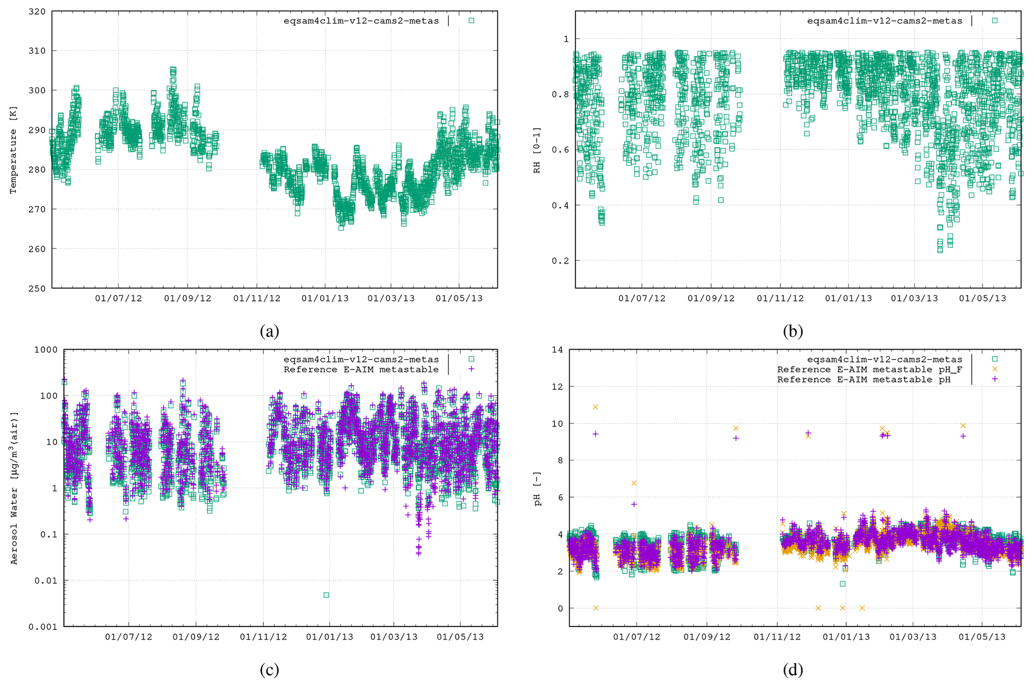
Figure 2The first case study is the CESAR site, Cabauw, the Netherlands, 2 May 2012–4 June 2013 (2646 data points). The results of EQSAM4Clim-v12 (green, squares) in comparison with E-AIM (pink, cross) using the data provided by Pye et al. (2020). Both models use the T [K] (a) and RH [0–1] (b) together with the lumped ion concentrations [µg m−3 (air)] of Mg2+, Ca2+, K+, Na+, , , and as input to calculate the aerosol water mass, H2O [µg m−3 (air)] (c) and aerosol pH [–] (d), assuming the metastable aerosol phase (no solid–liquid, only gas–liquid partitioning aerosol partitioning). Additionally, the E-AIM output for the free pH (pHF; orange cross) is included (see Pye et al., 2020).
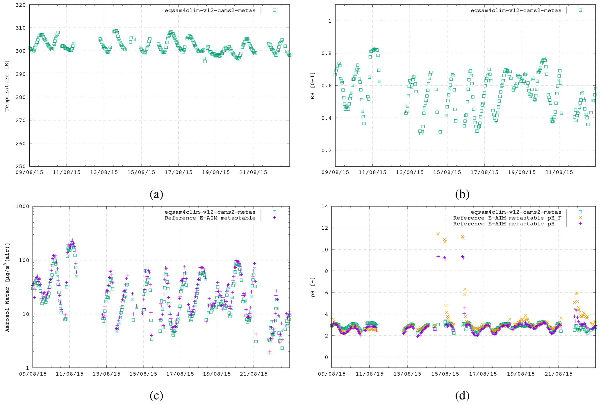
Figure 3The second case study is in Tianjin, China, 9–22 August 2015 (241 data points), using the following aerosol system:
Mg2+, Ca2+, K+, Na+, , , and .
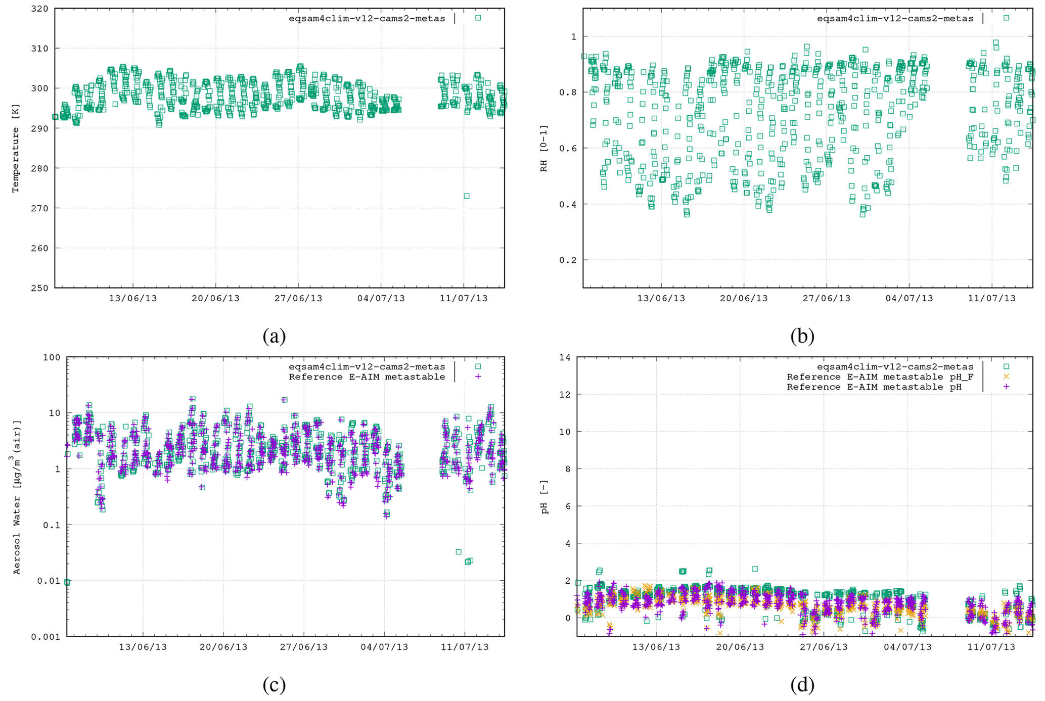
Figure 4The third case study is the SOAS campaign, Centreville, USA, 6 June–14 July 2013 (787 data points), using the following aerosol system: Na+, , , , .
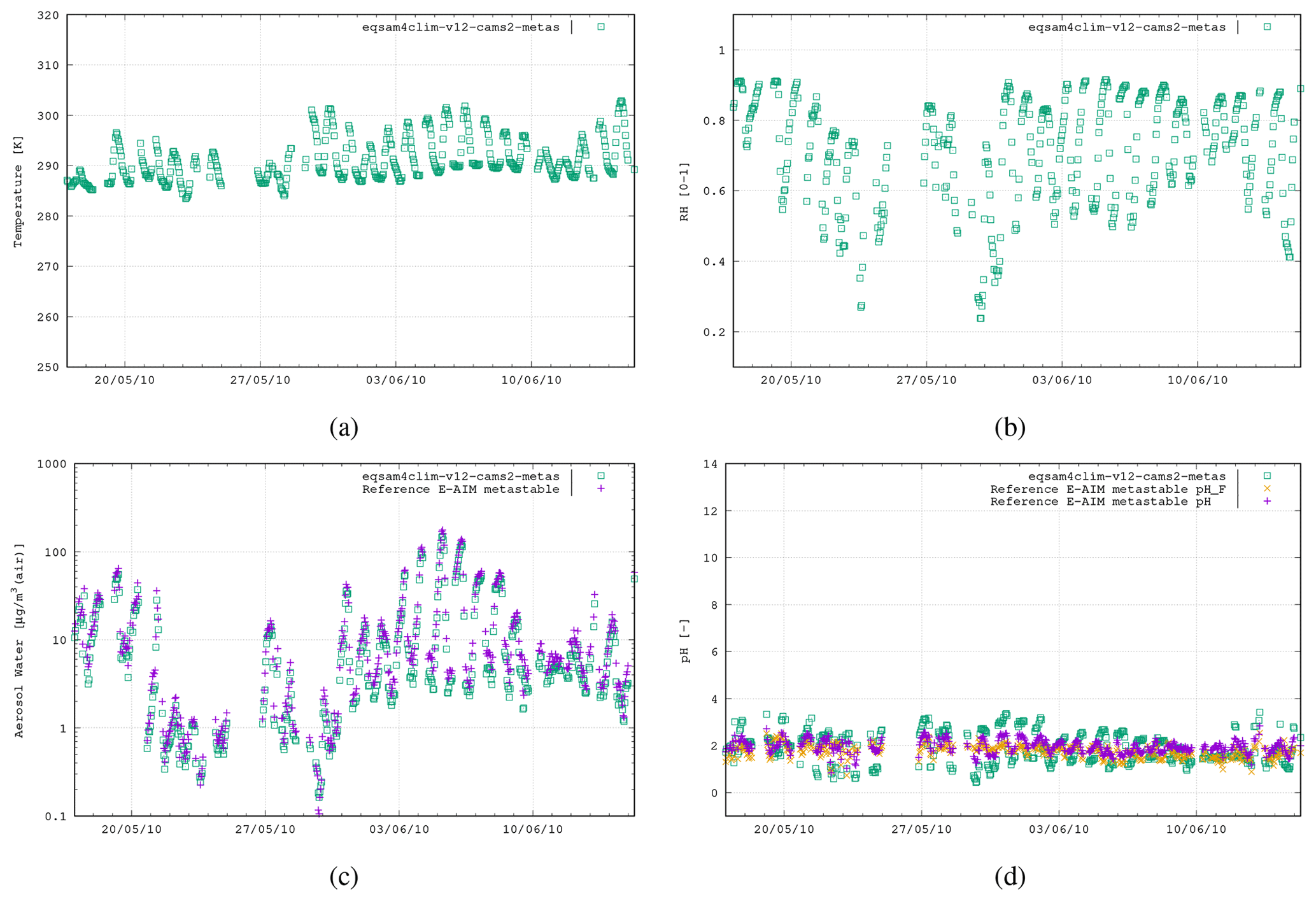
Figure 5The fourth case study is the CalNex campaign, Pasadena, CA, USA, 17 May–15 June 2010 (493 data points), using the following aerosol system: , , and .
Figures 3–5 show similar comparisons for summertime for the Tianjin (Shi et al., 2019), SOAS (Alabama Forest, USA; Guo et al., 2015) and CalNex (Pasadena, USA; Guo et al., 2017) campaigns, representing both urban and forest scenarios between the years 2010 and 2015. The range in T for these campaigns is typically limited to between 290–310 K, with distinct signatures of diurnal variability in the RH. These results show similar variability of AW content, with the pH range in SOAS (−1.0 to 2.0) being orders of magnitude more acidic than either CalNex (1.0–5.0) or Tianjin (2.0–5.0). Again, here, the spread in the pH values from EQSAM4Clim-v12 is similar to that of the E-AIM reference model and only a bit wider for the CalNex case compared to the Cabauw case, due to limitations of the partitioning of the EQSAM4Clim version. Currently this is the weakest part, and therefore the deviation in pH from E-AIM is largest. This will be subject to improvement in further updates.
Finally for wintertime under polluted conditions we use the data from one flight taken as part of the WINTER flight campaign (US East Coast; Guo et al., 2016). Here EQSAM4Clim-v12 is tested for lower temperatures across a wide range of RH values at various altitudes with high values of sea salt. Figure 6 shows comparisons using data from the flight taken on 3 February 2015. Both EQSAM4Clim-v12 pH and E-AIM simulate low pH values estimates, with similar variability and correlated well with respect to pH values <0.0. Note that the proposed parameterization does not show a limitation to very low or high RH values, according to the results shown. Also, extremely high RH values as high above 98–99 and even 100 %, which might be a meteorological input to EQSAM4Clim-v12 through a NWP coupling, are not a limiting factor in general. Instead, the representation of aerosol–cloud interactions and the dynamic limitations of gaseous uptake (including water vapor) might be here of primarily of concern, though the evaluation of EQSAM4Clim-v12 under such extreme RH regimes is beyond the scope of this study. In general, as RH approaches 100 %, one can anticipate increasing pH values, primarily driven by the corresponding increase in liquid water content. This rise in pH results from the dilution of H+ ions, leading to a reduction in acidity for a given H+ concentration. However, the situation becomes more complex in the presence of soluble gases that form acids, as the dissolution of acids can dampen the increase in pH. Additionally, factors such as the presence of ammonia, clouds, or precipitation further complicate this picture. For a more in-depth discussion on these intriguing aspects, we direct interested readers to the accompanying studies by Rémy et al. (2024) and Williams et al. (2024).
Figure 7 shows a comparison of the EQSAM4Clim-v12 pH results of the previous version 10 (left), used, e.g., in Fagerli et al. (2019) and Koo et al. (2020), with the current version 12 (right) versus the pH results of E-AIM for all five cases. Clearly, the pH results of EQSAM4Clim-v12 pH are closer to E-AIM compared to the v10, now more closely following the 1 : 1 line for a wide range of atmospheric conditions, although some scatter still remains. Note that this scatter is acceptable for the EQSAM4Clim parameterization concept. A more explicit treatment of the phase partitioning will be the subject of a follow-up study. Also note that both versions only differ by Eqs. (1)–(9e), with the results shown being sensitive to the Eq. (8) and the correction factors given in Table 1. Finally, note that what is most important for 3D applications is the fact that version 12 introduces a refined parameterization that separates the pH of aerosol, cloud and precipitation and addresses a limitation of previous versions through Eqs. (9a)–(9e). For a in-depth analysis we refer to the accompanying study of Rémy et al. (2024).
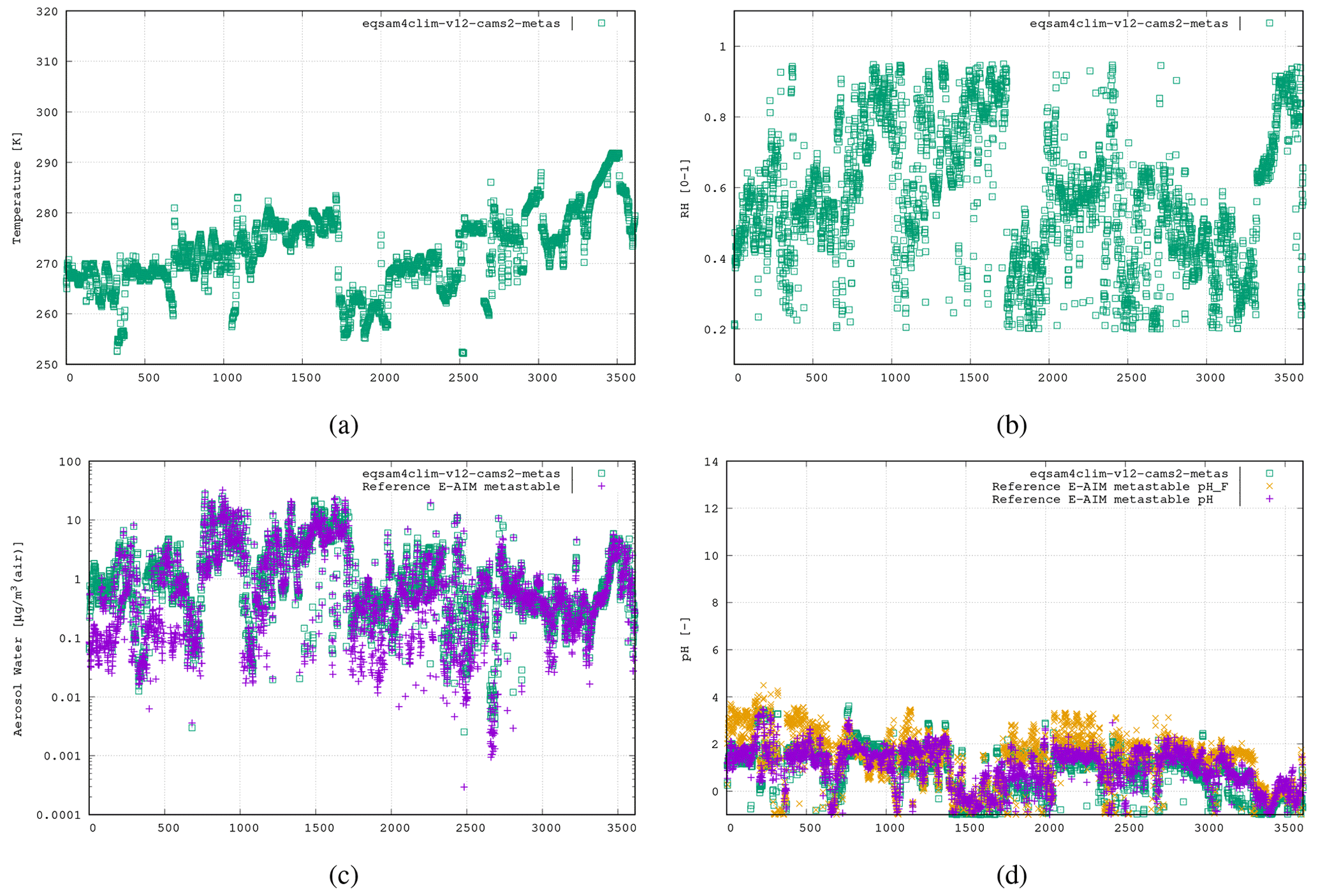
Figure 6The fifth case study is the WINTER campaign, US East Coast aloft, 3 February 2015, 3613 data points (real time axis; see Supplement), using the following aerosol system: , , , .
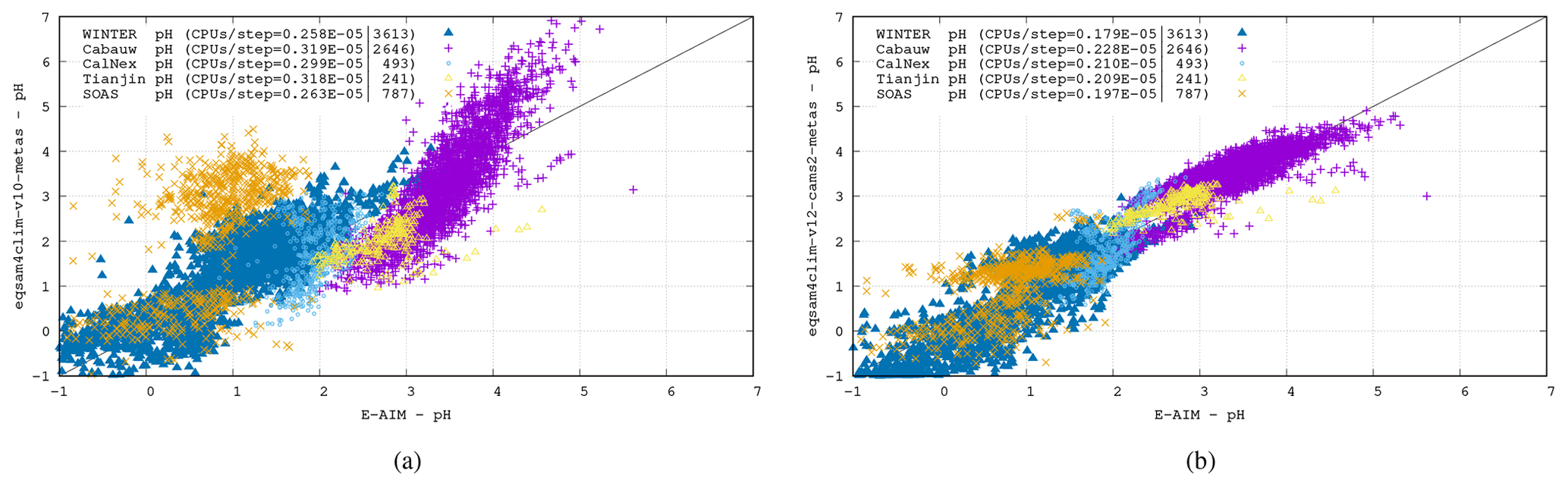
Figure 7Comparison of the EQSAM4Clim pH results of v10 (a) and v12 (b) versus the pH results of E-AIM for all five cases. The CPU consumption per step is included for each case. Chip: Apple M1 Ultra. Memory: 128 GB; llvm-11/flang compiler with O3.
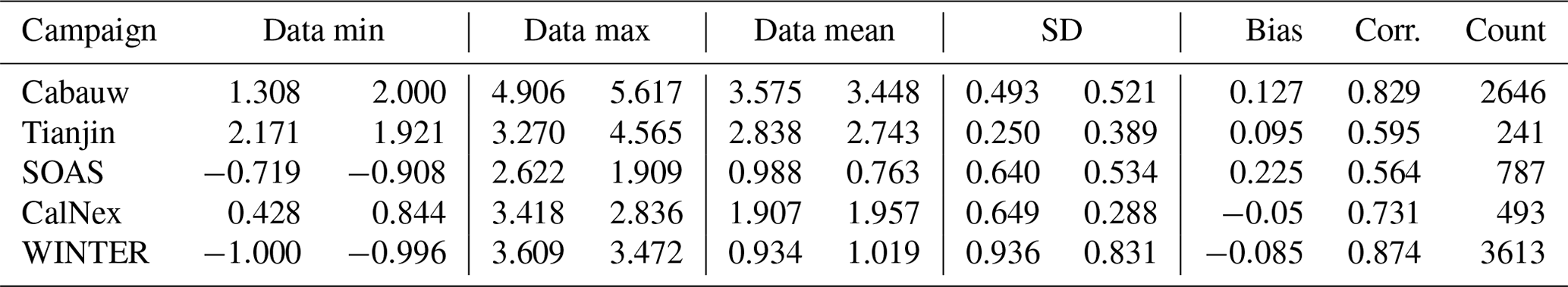
Table 2Statistical metrics for the pH results of EQSAM4Clim pH results of v12 (left) and E-AIM (right column).
To scrutinize the sensitivity and computational costs of these results, the results of two EQSAM4Clim versions including the CPU consumption per step are given in the panels of Fig. 7 for each case. Comparing the two EQSAM4Clim versions (left and right panel) shows that the pH results differ mostly for the Cabauw, Tianjin and SOAS campaigns, which represent different aerosol compositions and neutralization levels as defined by where the measurement campaign took place. The Cabauw and Tianjin campaigns represent the most complex aerosol system, with being fully neutralized (Sect. 3), since both locations are affected by anthropogenic precursors which undergo gas–aerosol partitioning. Conversely, data from the SOAS, Calnex and the WINTER campaigns represent cases where is not fully neutralized. In particular, the measurements from CalNex and the flight during the WINTER campaign represent often highly acidic cases.
Additionally, comparing the different campaign cases shows that the variability in the observed pH ranges across campaigns exceeds the variability in pH simulated by the different modeling code versions. For instance, for the WINTER campaign, the pH values are generally much lower compared to, e.g., the Cabauw campaign, which shows throughout all results the highest pH values, reflecting the predominance of cations in the aerosol system for the Cabauw case.
Table 2 summarizes the key metrics and shows the minimum and maximum pH value for each campaign, together with the data mean and standard deviation for EQSAM4Clim (v12) and E-AIM, as well as the correlation of both. While the data mean is generally satisfactorily close for all campaigns with a variation of less than 0.25 pH units, the correlation coefficient is only above 0.7 for the Cabauw, CalNex and WINTER campaign. Tianjin, which represents besides Cabauw the most complex aerosol system, shows a slightly lower correlation coefficient of 0.6, while SOAS is with a value of 0.56 at the lower end, due to the influence of sulfate–bisulfate partitioning. Bisulfates are not always captured in the gas–liquid partitioning compared to cases which include semi-volatile compounds (Cabauw, Tianjin, WINTER), but v12 still outperforms v10 (comparing Fig. 7a and b). Also note that the correlation coefficient is strongly influenced by the number of data points, such that the WINTER and Cabauw cases are statistically more significant.
This complexity of the Cabauw data is also reflected in the highest computing consumption per step (where CPU/step values are given in the legend within each panel of Fig. 7), while the WINTER campaign represents the least complex system (no cations and low temperatures) and, therefore, also requires the least CPU time. Note that there is some uncertainty in these numbers due to the load imbalance of the system (≤1 %), while the CPU consumption for EQSAM4Clim-v10 is higher due to the fact that double precision is used. For EQSAM4Clim-v12, the choice of precision is optional, and single precision is used throughout this work, since this alone can speed up the computations of up to 50 % for these run-time-optimized cases.
3.2 Application to IFS
Figure 8 extends Fig. 2 by showing an example of application and implementation of EQSAM4Clim-v12 into a comprehensive high-resolution atmospheric chemistry NWP forecasting system, with the chosen model being IFS-COMPO (Peuch et al., 2022). We use a version similar to that described in Rémy et al. (2022), where the gaseous precursors such as HNO3 are derived using the chemistry scheme given in Williams et al. (2022). The implementation provides global pH values, whose impact on aerosol composition and PM2.5 is evaluated in the accompanying study of Rémy et al. (2024). Here we only compare the new optional IFS pH results using a 3-hourly output frequency with those from the EQSAM4Clim-v12 and E-AIM box models at an hourly frequency for the Cabauw case as an example. Note that only a qualitative comparison is possible due to the cumulative effects of the different time averages, the difference in resolution (with IFS-COMPO being ran at ≈25 km scale) and the fact that the IFS-COMPO pH results are representative of 2019, while the box models show the results for the year 2012/2013. Nevertheless, overall, the seasonal trend of the pH values is captured rather well. During summertime (June–September) the IFS-COMPO pH values are on average less acidic than those calculated in the box models, while for the autumn and winter months, the agreement is on average very good. This evaluation furthermore illustrates that uncertainties to the input quantities (aerosol composition, relative humidity, temperature) dominate the overall uncertainty, indicating that EQSAM4Clim is fit for purpose.
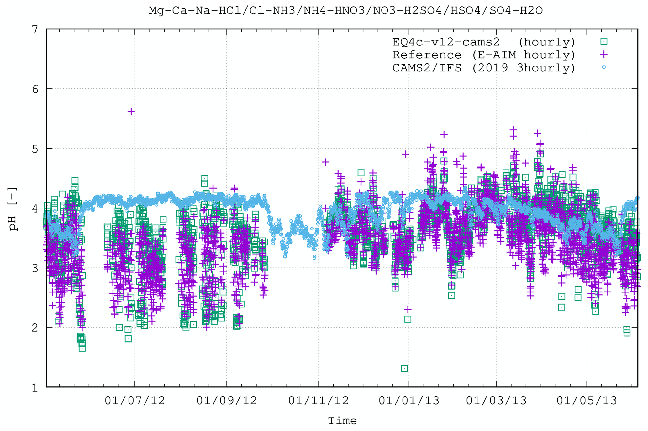
Figure 8Figure 2 extended to include IFS (3-hourly averages) in comparison with EQSAM4Clim-v12 and E-AIM box model results. Note that for this qualitative comparison, the simulation period for IFS is January to December 2019, while the box model results are shown for 2 May 2012 until 4 June 2013 (results are overlaid with matching seasons). All results are shown for the CESAR site at Cabauw (Fig. 2). A quantitative evaluation of the IFS-COMPO results is presented in the accompanying study of Rémy et al. (2024).
In this technical note, we have provided a description of the revised EQSAM4Clim-v12 pH parameterization developed for use in regional and global chemical forecasting systems. Using a range of diverse case studies, we have performed box model calculations, with the results being compared and calibrated against E-AIM upon introducing domain- and neutralization-dependent correction factors, i.e., KD and FN, respectively. The comparison against the E-AIM reference model calculations covers a range of seasons and scenarios ranging from forest measurements to maritime seaboard measurements. Generally, the pH values are mostly within the range given by E-AIM and now more closely following the 1 : 1 line for a wide range of atmospheric conditions compared to the previous EQSAM4Clim version (v10). Although some deviations of the EQSAM4Clim-v12 pH estimates are noted, the scatter is acceptable for the EQSAM4Clim parameterization concept. The case studies reveal that the pH results of the revised parameterization provide satisfactory representation for the most complex aerosol cases, i.e., the sulfate neutral conditions which are characterized by the gas–aerosol partitioning of semi-volatile ammonium compounds, while the less complex cases show a relatively larger scatter due to the limitations of the current partitioning parameterization. Overall, EQSAM4Clim has a low cost with respect to the total CPU consumption across aerosols with a range of composition complexity (as seen across different campaigns). This provides confidence that the revised pH parameterization is suitable for applications to large-scale chemical forecasting systems, where near-real-time results are mandatory. The accompanying study (Rémy et al., 2024) expands this evaluation to the global scale.
The current version of model is available from GitHub at https://github.com/rc-io/eqsam/tree/main (last access: 26 June 2024) under the licence CC-BY-SA-4.0. The exact version of the model used to produce the results used in this paper is archived on Zenodo (https://doi.org/10.5281/zenodo.10276178, Metzger, 2023), as are input data and scripts to run the model and produce the plots for all the simulations presented in this paper (Metzger, 2023).
The supplement related to this article is available online at: https://doi.org/10.5194/gmd-17-5009-2024-supplement.
SM drafted the paper and developed and implemented the revised pH formulation of EQSAM4Clim-v12 into IFS. SR, VH, SM, JEW and JF maintain and carry out general aerosol and trace gas developments on IFS-COMPO; and all authors contributed to drafting and revising this article.
At least one of the (co-)authors is a member of the editorial board of Geoscientific Model Development. The peer-review process was guided by an independent editor, and the authors also have no other competing interests to declare.
Publisher's note: Copernicus Publications remains neutral with regard to jurisdictional claims made in the text, published maps, institutional affiliations, or any other geographical representation in this paper. While Copernicus Publications makes every effort to include appropriate place names, the final responsibility lies with the authors.
This work is supported by the Copernicus Atmospheric Monitoring Services (CAMS) program managed by ECMWF on behalf of the European Commission. We acknowledge the Pye et al. (2020) study for providing the data of the box modeling study.
This paper was edited by Klaus Klingmüller and reviewed by two anonymous referees.
Fagerli, H., Tsyro, S., Jonson, J. E., Nyíri, Á., Gauss, M., Simpson, D., Wind, P., Benedictow, A., Klein, H., Mortier, A., Aas, W., Hjellbrekke, A.-G., Solberg, S., Platt, S. M., Yttri, K. E., Tørseth, K., Gaisbauer, S., Mareckova, K., Matthews, B., Schindlbacher, S., Sosa, C., Tista, M., Ullrich, B., Wankmüller, R., Scheuschner, T., Bergström, R., Johanson, L., Jalkanen, J.-P., Metzger, S., Denier van der Gon, H. A. C., Kuenen, J. J. P., Visschedijk, A. J. H., Barregård, L., Molnár, P., and Stockfelt, L.: Transboundary particulate matter, photo-oxidants, acidifying and eutrophying components, EMEP Status Report 1 “, Norwegian Meteorological Institute, https://emep.int/publ/reports/2019/EMEP_Status_Report_1_2019.pdf (last access: 26 June 2024), 2019. a, b
Flemming, J., Huijnen, V., Arteta, J., Bechtold, P., Beljaars, A., Blechschmidt, A.-M., Diamantakis, M., Engelen, R. J., Gaudel, A., Inness, A., Jones, L., Josse, B., Katragkou, E., Marecal, V., Peuch, V.-H., Richter, A., Schultz, M. G., Stein, O., and Tsikerdekis, A.: Tropospheric chemistry in the Integrated Forecasting System of ECMWF, Geosci. Model Dev., 8, 975–1003, https://doi.org/10.5194/gmd-8-975-2015, 2015. a, b
Friese, E. and Ebel, A.: Temperature Dependent Thermodynamic Model of the System H+-NH-Na+-SO-NO-Cl−-H2O, J. Phys. Chem. A, 114, 11595–11631, https://doi.org/10.1021/jp101041j, 2010. a
Guo, H., Xu, L., Bougiatioti, A., Cerully, K. M., Capps, S. L., Hite Jr., J. R., Carlton, A. G., Lee, S.-H., Bergin, M. H., Ng, N. L., Nenes, A., and Weber, R. J.: Fine-particle water and pH in the southeastern United States, Atmos. Chem. Phys., 15, 5211–5228, https://doi.org/10.5194/acp-15-5211-2015, 2015. a
Guo, H., Sullivan, A. P., Campuzano-Jost, P., Schroder, J. C., Lopez-Hilfiker, F. D., Dibb, J. E., Jimenez, J. L., Thornton, J. A., Brown, S. S., Nenes, A., and Weber, R. J.: Fine particle pH and the partitioning of nitric acid during winter in the northeastern United States, J. Geophys. Res.-Atmos., 121, 10355–10376, https://doi.org/10.1002/2016JD025311, 2016. a
Guo, H., Liu, J., Froyd, K. D., Roberts, J. M., Veres, P. R., Hayes, P. L., Jimenez, J. L., Nenes, A., and Weber, R. J.: Fine particle pH and gas–particle phase partitioning of inorganic species in Pasadena, California, during the 2010 CalNex campaign, Atmos. Chem. Phys., 17, 5703–5719, https://doi.org/10.5194/acp-17-5703-2017, 2017. a
Guo, H., Otjes, R., Schlag, P., Kiendler-Scharr, A., Nenes, A., and Weber, R. J.: Effectiveness of ammonia reduction on control of fine particle nitrate, Atmos. Chem. Phys., 18, 12241–12256, https://doi.org/10.5194/acp-18-12241-2018, 2018. a
Huijnen, V., Le Sager, P., Köhler, M. O., Carver, G., Rémy, S., Flemming, J., Chabrillat, S., Errera, Q., and van Noije, T.: OpenIFS/AC: atmospheric chemistry and aerosol in OpenIFS 43r3, Geosci. Model Dev., 15, 6221–6241, https://doi.org/10.5194/gmd-15-6221-2022, 2022. a
Koo, B., Metzger, S., Vennam, P., Emery, C., Wilson, G., and Yarwood, G.: Comparing the ISORROPIA and EQSAM Aerosol Thermodynamic Options in CAMx, in: Air Pollution Modeling and its Application XXVI, series Title: Springer Proceedings in Complexity, edited by Mensink, C., Gong, W., and Hakami, A., Springer International Publishing, Cham, 93–98, ISBN 978-3-030-22054-9 978-3-030-22055-6, https://doi.org/10.1007/978-3-030-22055-6_16, 2020. a, b
Metzger, S.: The EQSAM Box Model (for eqsam4clim-v12), Zenodo [code and data set], https://doi.org/10.5281/zenodo.10276178, 2023. a, b
Metzger, S., Dentener, F., Pandis, S., and Lelieveld, J.: Gas/aerosol partitioning: 1. A computationally efficient model, J. Geophys. Res.-Atmos., 107, ACH 16-1–ACH 16-24, https://doi.org/10.1029/2001JD001102, 2002. a
Metzger, S., Steil, B., Xu, L., Penner, J. E., and Lelieveld, J.: New representation of water activity based on a single solute specific constant to parameterize the hygroscopic growth of aerosols in atmospheric models, Atmos. Chem. Phys., 12, 5429–5446, https://doi.org/10.5194/acp-12-5429-2012, 2012. a, b, c, d
Metzger, S., Abdelkader, M., Klingmueller, K., Steil, B., and Lelieveld, J.: Comparison of Metop PMAp Version 2 AOD Products using Model Data, final Report ITT 15/210839, EUMETSAT, https://www.eumetsat.int/PMAp (last access: 26 June 2024), 2016a. a, b
Metzger, S., Steil, B., Abdelkader, M., Klingmüller, K., Xu, L., Penner, J. E., Fountoukis, C., Nenes, A., and Lelieveld, J.: Aerosol water parameterisation: a single parameter framework, Atmos. Chem. Phys., 16, 7213–7237, https://doi.org/10.5194/acp-16-7213-2016, 2016b. a, b, c, d, e, f, g, h, i, j, k
Metzger, S., Abdelkader, M., Steil, B., and Klingmüller, K.: Aerosol water parameterization: long-term evaluation and importance for climate studies, Atmos. Chem. Phys., 18, 16747–16774, https://doi.org/10.5194/acp-18-16747-2018, 2018. a, b, c, d
Metzger, S., Remy, S., Williams, J. E., Huijnen, V., Meziane, M., Kipling, Z., Flemming, J., and Engelen, R.: Representing acidity in the IFS using a coupled IFS-EQSAM4Clim approach, EGU General Assembly 2022, Vienna, Austria, 23–27 May 2022, EGU22-11122, https://doi.org/10.5194/egusphere-egu22-11122, 2022. a
Metzger, S., Rémy, S., Huijnen, V., Williams, J., Chabrillat, S., Bingen, C., and Flemming, J.: Impact of pH computation from EQSAM4Clim on inorganic aerosols in the CAMS system, EGU General Assembly 2023, Vienna, Austria, 24–28 April 2023, EGU23-16085, https://doi.org/10.5194/egusphere-egu23-16085, 2023. a
Peuch, V.-H., Engelen, R., Rixen, M., Dee, D., Flemming, J., Suttie, M., Ades, M., Agusti-Panareda, A., Ananasso, C., Andersson, E., Armstrong, D., Barre, J., Bousserez, N., Dominguez, J. J., Garrigues, S., Inness, A., Jones, L., Kipling, Z., Letertre-Danczak, J., Parrington, M., Razinger, M., Ribas, R., Vermoote, S., Yang, X., Simmons, A., de Marcilla, J. G., and Thepaut, J.-N.: The Copernicus Atmosphere Monitoring Service: From Research to Operations, B. Am. Meteorol. Soc., 103, E2650–E2668, https://doi.org/10.1175/BAMS-D-21-0314.1, 2022. a, b
Pye, H. O. T., Nenes, A., Alexander, B., Ault, A. P., Barth, M. C., Clegg, S. L., Collett Jr., J. L., Fahey, K. M., Hennigan, C. J., Herrmann, H., Kanakidou, M., Kelly, J. T., Ku, I.-T., McNeill, V. F., Riemer, N., Schaefer, T., Shi, G., Tilgner, A., Walker, J. T., Wang, T., Weber, R., Xing, J., Zaveri, R. A., and Zuend, A.: The acidity of atmospheric particles and clouds, Atmos. Chem. Phys., 20, 4809–4888, https://doi.org/10.5194/acp-20-4809-2020, 2020. a, b, c, d, e, f, g, h, i, j
Rémy, S., Kipling, Z., Huijnen, V., Flemming, J., Nabat, P., Michou, M., Ades, M., Engelen, R., and Peuch, V.-H.: Description and evaluation of the tropospheric aerosol scheme in the Integrated Forecasting System (IFS-AER, cycle 47R1) of ECMWF, Geosci. Model Dev., 15, 4881–4912, https://doi.org/10.5194/gmd-15-4881-2022, 2022. a, b
Rémy, S., Metzger, S., Huijnen, V., Williams, J. E., and Flemming, J.: An improved representation of aerosol acidity in the ECMWF IFS-COMPO 49R1 through the integration of EQSAM4Climv12, EGUsphere [preprint], https://doi.org/10.5194/egusphere-2023-3072, 2024. a, b, c, d, e, f, g, h
Shi, X., Nenes, A., Xiao, Z., Song, S., Yu, H., Shi, G., Zhao, Q., Chen, K., Feng, Y., and Russell, A. G.: High-Resolution Data Sets Unravel the Effects of Sources and Meteorological Conditions on Nitrate and Its Gas-Particle Partitioning, Environ. Sci. Technol., 53, 3048–3057, https://doi.org/10.1021/acs.est.8b06524, 2019. a
Wexler, A. S. and Clegg, S. L.: Atmospheric aerosol models for systems including the ions H+, NH4+, Na+, SO42−, NO3−, Cl−, Br−, and H2O, J. Geophys. Res.-Atmos., 107, ACH 14-1–ACH 14-14, https://doi.org/10.1029/2001JD000451, 2002. a
Williams, J. E. ., Huijnen, V., Bouarar, I., Meziane, M., Schreurs, T., Pelletier, S., Marécal, V., Josse, B., and Flemming, J.: Regional evaluation of the performance of the global CAMS chemical modeling system over the United States (IFS cycle 47r1), Geosci. Model Dev., 15, 4657–4687, https://doi.org/10.5194/gmd-15-4657-2022, 2022. a
Williams, J. E., Rémy, S., Metzger, S., Huijnen, V., and Flemming, J.: An evaluation of the regional distribution and wet deposition of secondary inorganic aerosols and their gaseous precursors in IFS-COMPO 49R1: the impact of aerosol and cloud pH, in preparation, 2024. a
- Article
(8617 KB) - Full-text XML