REHEATFUNQ (REgional HEAT-Flow Uncertainty and aNomaly Quantification) 2.0.1: a model for regional aggregate heat flow distributions and anomaly quantification

Surface heat flow is a geophysical variable that is affected by a complex combination of various heat generation and transport processes. The processes act on different lengths scales, from tens of meters to hundreds of kilometers. In general, it is not possible to resolve all processes due to a lack of data or modeling resources, and hence the heat flow data within a region is subject to residual fluctuations.

We introduce the REgional HEAT-Flow Uncertainty and aNomaly Quantification (REHEATFUNQ) model, version 2.0.1. At its core, REHEATFUNQ uses a stochastic model for heat flow within a region, considering the aggregate heat flow to be generated by a gamma-distributed random variable. Based on this assumption, REHEATFUNQ uses Bayesian inference to (i) quantify the regional aggregate heat flow distribution (RAHFD) and (ii) estimate the strength of a given heat flow anomaly, for instance as generated by a tectonically active fault. The inference uses a prior distribution conjugate to the gamma distribution for the RAHFDs, and we compute parameters for a uninformed prior distribution from the global heat flow database by Lucazeau (2019). Through the Bayesian inference, our model is the first of its kind to consistently account for the variability in regional heat flow in the inference of spatial signals in heat flow data. Interpretation of these spatial signals and in particular their interpretation in terms of fault characteristics (particularly fault strength) form a long-standing debate within the geophysical community.

We describe the components of REHEATFUNQ and perform a series of goodness-of-fit tests and synthetic resilience analyses of the model. While our analysis reveals to some degree a misfit of our idealized empirical model with real-world heat flow, it simultaneously confirms the robustness of REHEATFUNQ to these model simplifications.

We conclude with an application of REHEATFUNQ to the San Andreas fault in California. Our analysis finds heat flow data in the Mojave section to be sufficient for an analysis and concludes that stochastic variability can allow for a surprisingly large fault-generated heat flow anomaly to be compatible with the data. This indicates that heat flow alone may not be a suitable quantity to address fault strength of the San Andreas fault.

1 Introduction

Surface heat flow is an important geophysical parameter. It plays an important role in the global energy budget of the solid Earth (Davies and Davies, 2010) and has implications for the exploitability of geothermal energy as a renewable energy source (e.g., Moya et al., 2018). It is also intimately connected to the crustal temperature field which has the potential to control the crustal elastic properties (Peña et al., 2020) and is hence vital for the understanding of seismic and aseismic crustal deformation. Furthermore, measurements of the surface heat flow have been indicative of the frictional strength of the San Andreas fault (SAF) by constraining the heat production rate on the fault surface (Brune et al., 1969; Lachenbruch and Sass, 1980).

Global patterns of surface heat flow have been investigated in multiple works (e.g., Pollack et al., 1993; Goutorbe et al., 2011; Lucazeau, 2019). The models therein usually assign an average heat flow to each point of Earth's surface, for instance by dividing the surface into a grid. We denote this as the “background heat flow” q_b, which might follow from the two main sources of crustal heat flow, mantle heat transmission and radiogenic heat generation (Gupta, 2011). As data accumulated, the additional information was used in later works to improve the spatial resolution of q_b models.

Alas, even at the finer resolution of newer works, the models of global heat flow do not perfectly describe the heat flow measurements due to fluctuations. Goutorbe et al. (2011) observe that a residual variation of 10 to 20 mW m⁻² remains between heat flow measurements not further than 50 km apart. One potential cause of this variation is the varying concentration of radiogenic elements within the upper crust, which has been observed to change by a factor of 5 within a couple of tens of meters (Landström et al., 1980; Jaupart and Mareschal, 2005).

Whatever the cause, the magnitude of the variation observed by Goutorbe et al. (2011) and its spatial extent are similar to some anomalous signals generated by processes that one might wish to investigate and distinguish from the background q_b. The fault-generated heat flow anomaly discussed by Lachenbruch and Sass (1980) regarding the SAF, with a peak heat flow less than about 27 mW m⁻², is an important example. The magnitude similarity between the residual variation and the queried signature implies that it is difficult to establish bounds on the latter.

In this article, we introduce the REHEATFUNQ model (REgional HEAT Flow Uncertainty and aNomaly Quantification), which aims to

1. quantify the variability within regional heat flow measurements and

2. identify how strong the surface heat flow signature of a deterministic process, e.g., fault-generated heat flow, can be given a set of heat flow measurements in the study area.

REHEATFUNQ approaches these goals by aggregating heat flow measurements in a region of interest (ROI) into a location-agnostic distribution of heat flow. It considers the heat flow within the region as the result of a stochastic process and hence the aggregate distribution as the probability distribution of a random variable. In a Bayesian workflow, this distribution is inferred from the regional heat flow data and from prior information. Processes such as the fault-generated surface heat flow can be quantified by supplying the impact of the process onto each data point and inferring the posterior distribution of a process strength parameter.

The REHEATFUNQ model is an empirical model. In this study, we have performed a number of analyses of the New Global Heat Flow (NGHF) database by Lucazeau (2019) to inform the model. Synthetic computer simulations based on the REHEATFUNQ model assumptions have been performed to test the model performance on ideal data. We also perform a resilience analysis based on a number of alternatives to the model assumptions which are also compatible with the NGHF database.

The paper starts with a description of the (heat flow) basis data of the REHEATFUNQ model in Sect. 2. The methodology section (Sect. 3) continues with a physical motivation for the REHEATFUNQ model before it transitions to a technical description of the model's capabilities. Section 4 bundles statistical analyses of the performance of the REHEATFUNQ model and is rather technical. It starts out by assessing how well the model assumptions are reflected in real-world data, uses stochastic computer simulations to investigate whether known imperfections inhibit REHEATFUNQ's usefulness, and discusses physical limitations of the model. Section 5 then illustrates how to apply the REHEATFUNQ model by means of the San Andreas fault in Southern California before Sect. 6 concludes this work. As a reference for the application of the REHEATFUNQ model, Appendix A summarizes all analysis steps mentioned throughout the paper in a workflow cheat sheet.

2 Heat flow data

This work is fundamentally built on the analysis of surface heat flow measurements, that is, point measurements of the flow of thermal energy from Earth's interior through the outermost layer of the crust into the atmosphere. Heat flow has units of energy divided by time and area; integrated over an area of Earth's surface, it gives the power at which thermal energy transfers from the inside to the atmosphere.

Heat flow is typically estimated from temperature measurements at varying depths within a borehole. From these measurements, the temperature gradient is estimated which, multiplied with the heat conductivity of the surrounding rock, leads to the heat flow estimate (e.g., Henyey and Wasserburg, 1971). For more details, we refer the reader, for instance, to Henyey and Wasserburg (1971), Fulton et al. (2004), and Sass and Beardsmore (2011).

Measuring heat flow is a difficult task. Each measurement requires a borehole and sufficient time to establish temperature equilibrium at the sensors (Henyey and Wasserburg, 1971). Furthermore, the temperature profile close to Earth's surface might not be linear with depth, as would be imposed by a constant heat flow. The causes for these perturbations can include topography, erosion, climate, and water circulation (Lucazeau, 2019), the latter as advection or convection. These perturbations have to be corrected for to estimate the crustal heat flow component of the measured temperature profile. Otherwise crustal heat flow estimates will be biased or uncertain.

Heat flow data are multidimensional, spanning most prominently the heat flow as well as the spatial dimensions. Within the REHEATFUNQ model, the heat flow data are aggregated within the region of interest (ROI) and investigated without regard for the further spatial distribution. We call this data set, reduced to the heat flow dimension only, the regional aggregate heat flow distribution. Formally, given a set $\mathit{\left\{}\right({\mathit{x}}_i,q_i):i=\mathrm{1},\mathrm{\dots },N\mathit{\}}$ of heat flow measurements within a ROI, one may write the regional aggregate heat flow distribution as result of the mapping:

$$\begin{array}{}\text{(1)}& \mathit{\left\{}\right({\mathit{x}}_i,q_i):i=\mathrm{1},\mathrm{\dots },N\mathit{\}}\to \mathit{\{}{q}_i:i=\mathrm{1},\mathrm{\dots },N\mathit{\}}.\end{array}$$

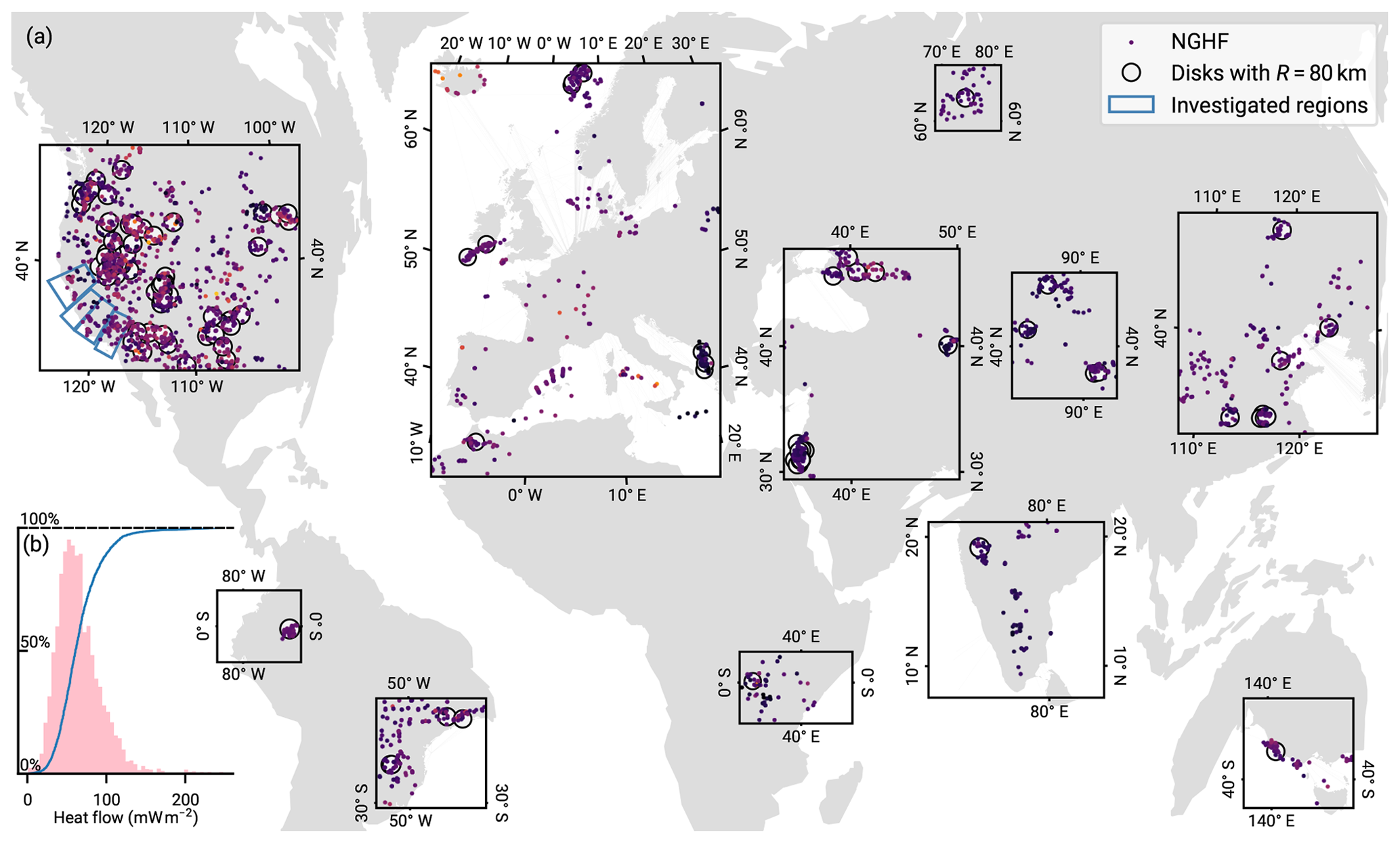
Figure 1 New Global Heat Flow (NGHF) database (Lucazeau, 2019) and random regional heat flow samples. The map shows data points from the NGHF used in this study, corresponding to positive continental heat flow values with a quality ranking of “A” to “B” and not exceeding 250  mW m⁻². The set of random global R-disk coverings (RGRDCs) used in Sect. 3.3.2 to determine the estimates of the prior distribution parameters is illustrated by thinly outlined disks. The algorithm to distribute the disks is described in Appendix B. The analysis regions used in Sect. 5 for the SAF are shown in a thicker blue outline. Inset (b): empirical distribution function and histogram of the same global heat flow data.

2.1 Data used and general filtering

In this work, we build upon a global database of heat flow measurements compiled by Lucazeau (2019), the NGHF. This data set, a continuation of the effort of Pollack et al. (1993), is a heterogeneous collection of 69 730 heat flow measurements from a variety of studies. It covers the time period from 1939 to 2019 and covers the globe on multiple spatial scales from repeat measurements at the same location up to the largest nearest-neighbor distances of ∼1200 km. We will use both the global coverage as well as the specific region of Southern California in this work. Due to the heterogeneous spatial coverage and quality of the data, we apply a number of data filters beforehand.

We use only a quality-filtered subset of the NGHF in all our following analyses. Lucazeau (2019) compiled heat flow data from a wide range of sources, spanning decades of technological improvements in instrumentation and combining various work on perturbation correction and uncertainty estimation. To obtain more homogeneous data quality, we follow the quality assessment described by Lucazeau (2019) and discard data points of the lowest quality rankings of C to F and those from earlier than 1990 (marking an increase in data quality). We furthermore remove negative heat flow values.

Since we will consider a continental scenario, we furthermore remove data points not marked as continental crust (i.e. not keys A to H in field “code1”). Finally, we discard data points categorized as possibly geothermal following Lucazeau (2019), that is, those exceeding 250 mW m⁻². The remaining data set has 5974 entries. The global aggregate heat flow distribution of this remaining data set is shown in Fig. 1.

The filtering steps described in this section are an example of what is subsumed as step 1 of the workflow listed in Appendix A.

3 Methodology: a stochastic model of regional aggregate heat flow

3.1 Physical basis

Surface heat flow is the result of heat, generated in Earth's interior, being transported to the surface by diffusive, advective, and convective processes. The main sources of heat within Earth are the thermal energy from its planetary genesis and the decay of radioactive elements (Christensen, 2011; Mareschal and Jaupart, 2021). Within the crust, heat production due to the friction on faults can be large enough to cause measurable local disturbances of the temperature field (e.g., Kano et al., 2006) and could potentially also lead to significant disturbances in the surface heat flow field if the frictional strength of the fault were large (Brune et al., 1969; Lachenbruch and Sass, 1980).

After generation, three modes of steady transport can be available to bring the heat to the surface. Heat diffusion occurs throughout Earth's interior. Advection can occur with the tectonic movement of rock or by means of gravitationally driven pore water movement (Molnar and England, 1990; Fulton et al., 2004). Convective processes range from magma convection in the mantle through crustal pore water convection (Bercovici and Mulyukova, 2021; Hewitt, 2020).

Both generation and transport of heat within Earth are subject to a number of unknowns such as material composition in terms of heat generation and conduction, the geometry of convection cells, and the existence of groundwater flow (e.g., Morgan, 2011). Some of these parameters are difficult to determine, and typically residual fluctuations remain in thermal models even if those models take into account a multitude of available information (e.g., Cacace et al., 2013; Fulton et al., 2004). That is, even though the principles underlying the full surface heat flow field are known, the incomplete knowledge of the specific crustal processes and material properties defining a specific region's surface heat flow, in combination with measurement uncertainties, makes it generally impossible to model the exact surface heat flow that is measured.

Our approach is to acknowledge that a model is unlikely to capture the full surface heat flow signal simply because the input data do not capture all relevant features of the subsurface or because the measurement is uncertain. The concept of REHEATFUNQ is then to abstract these unknowns into a black-box stochastic model of surface heat flow within a region. The stochastic model condenses the spatial distribution of heat flow into a single probability distribution of heat flow q, γ(q), for the whole region, agnostic to where heat flow is queried within. This way, unknowns about the parameters that control surface heat flow are captured by the amount and variance of the measurement data. If a region is characterized by uniform heat flow – that is, it is independent and identically distributed following a single distribution γ(q) – and sufficient data have been collected, a statistical analysis will yield a precise result. Variability in the heat flow controlling parameters reflects in a wider spread of the inferred distribution instead.

The arguments that motivate the REHEATFUNQ approach are related to the spatial variability in heat flow. Surface heat flow exhibits variability on a large range of scales. Long-wavelength contributions follow from the diffusion from deep heat sources. The diffusion up to the crustal surface smoothes the lateral pattern of heat flow from these sources with a characteristic length of 100 km (Jaupart and Mareschal, 2005, 2007). If the resulting signal does not vary significantly within the extent of the ROI, we label it the locally uniform background q_b. In our later analysis, the extent will be ∼160 km, but this is not a hard constraint on the region size.

The surface heat flow also contains signals of a smaller spatial scale, say 50–100 km and below. We label the surface heat flow that varies spatially within the ROI with q_s(x). Examples of these short-wavelength effects include radiogenic heat production from the tens-of-meters to kilometer scale (Jaupart and Mareschal, 2005) or recent tectonic history through movement of heated mass or friction on faults (Morgan, 2011).

One type of short-wavelength signal is topographic effects. Since they are more readily corrected for Blackwell et al. (e.g., 1980) and Fulton et al. (2004), we list them separately as q_t(x). Topographic effects act on the scale of hundreds of meters to multiple kilometers (see, e.g., the extent of the mountains listed by Blackwell et al., 1980) if the boreholes are not sufficiently deep (that is, shallower than 75–300 m depending on temperature gradient and topographic variability; Blackwell et al., 1980).

Finally, the heat flow might also be influenced by random measurement error q_f. This includes all kinds of difficulties inherent to the process of drilling, measuring temperature, and evaluating heat flow gradients. These effects are independent of location.

All these unknown contributions to the surface heat flow complicate the inference of a known constituent of the heat flow signal from the data. For instance, one might have good knowledge about the location of an underground heat source and its heat transport to the surface and hence be able to accurately model the spatial surface heat flow signature q_a(x) that the heat source generates but might not know about the heat source's strength and hence the magnitude of the signature. The quantification of fault-generated heat flow anomalies on the San Andreas fault is a paragon of this problem (Brune et al., 1969; Lachenbruch and Sass, 1980; Fulton et al., 2004) and is the inspiration behind the name q_a (“anomaly”). Because the surface heat flow is influenced by many unknown effects – unknown but evident due to the variability that is not perfectly fit by the model's signature – it is not trivial to infer the magnitude of the model's heat source. This applies particularly if the magnitude of the signature generated by the actual heat source is on the order of or less than the spread due to the unknown constituents.

REHEATFUNQ aims to solve this issue through the stochastic model of the unknown constituents of surface heat flow and consequently to help researchers calibrate models of specific surface heat flow constituents. The surface heat flow field q(x) is separated into the modeled heat flow q_a(x) and the unknown contributions q_b, q_s(x), q_t(x), and q_f. The magnitude of the modeled heat flow q_a(x) is expressed in terms of the power P_H of the heat source (an example is given later in Sect. 3.4.1), and a Bayesian inference of this parameter is performed using heat flow measurements q_i, that is, samples of the unknown stochastic constituents transformed to q(x) when combined with q_a(x). Before the following sections discuss the stochastic model and the inference of the magnitude of q_a, we discuss the separation of q_a from the unknown constituents and, equivalently, how the stochastic model and the modeled heat flow relate to the heat flow measurements.

If heat transport in the crust is linear, which is the case for conduction and advection, the heat flow q(x) is a superposition of the five constituents:

$$\begin{array}{}\text{(2)}& q\left(\mathit{x}\right)=\underset{q_{\mathrm{u}}\left(\mathit{x}\right)}{\underbrace{q_{\mathrm{b}}+q_{\mathrm{s}}\left(\mathit{x}\right)+q_{\mathrm{t}}\left(\mathit{x}\right)+q_{\mathrm{f}}}}+q_{\mathrm{a}}\left(\mathit{x}\right).\end{array}$$

Here, we have collected all these unknowns into q_u(x). If heat transport is nonlinear, for instance in the case of nonlinear convection, a superposition like this would not be possible. Instead, q(x) would be a nonlinear function of the sources of q_b, q_s, q_t, q_f, and q_a. If the heat source that causes the anomaly q_a is itself a driver of the convection, REHEATFUNQ as developed in this paper cannot be applied (with one technical exception mentioned further down in Appendix G, whose applicability is unclear). This might not be a significant restriction, however: if the heat source that generates the anomaly q_a is strong enough to drive convection on significant length scales (that is, the 1–10 km scale), the resulting surface heat flow signature is probably large enough (that is, more than 50–100 mW m⁻²) for the separation from the “background noise” (the undisturbed heat flow) to be less challenging.

However, if the magnitude of q_a is small (that is, less than about 50–100 mW m⁻²), the need for a statistical method, such as REHEATFUNQ, is essential. In the case of a small q_a with a crustal heat source, the source will be similarly small and likely not be a driver of convection. Then, if some of the other heat sources, underlying q_b, q_s, q_t, and q_f, drive nonlinear convective transport, a linearization of the heat transport equation similar to the one performed by Bringedal et al. (2011) can be performed, which would again separate q_a as a linear constituent of q(x) from the unknown:

$$\begin{array}{}\text{(3)}& q\left(\mathit{x}\right)=q_{\mathrm{u}}\left(\mathit{x}\right)+q_{\mathrm{a}}\left(\mathit{x}\right).\end{array}$$

Illustratively, the nonlinear convection due to other sources would act as an advective term for the diffusion advection of the anomalous heat source.

Equation (3) shows the extent of separation that is required for REHEATFUNQ to be applied. It enables the linear separation of the model output from the unknown heat flow which is treated by the stochastic approach. But what motivates the stochastic approach, describing q_u as a probability distribution γ(q_u)?

For the error term q_f, the treatment as a random variable is straightforward. To treat the other terms stochastically is less evident since the surface heat flow field should in principle be deterministic and accessible through a precise measurement given enough effort. Here we can consider the random location sampling of a deterministic q_u landscape as a stochastic source of the q_u random variable. Figure 2 illustrates this approach. The surface heat flow field acts like a random variable transform of the spatial random variable to the random variable q. The probability density of q derives from the level set of the heat flow field.

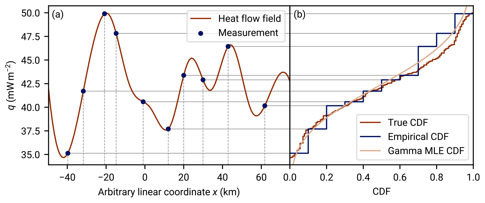
Figure 2 The stochastic model of regional aggregate heat flow from a deterministic surface heat flow field: an artificial illustration. (a) An artificial one-dimensional surface heat flow field generated from artificial underground heat sources. The underground heat sources (200 km wide, 80 km deep grid with 201×151 cells, not shown) have been optimized from random initial values such that the surface heat flow they generate fits a target heat flow distribution whose aggregate distribution is close to a gamma distribution (details in Appendix F). The blue dots illustrate heat flow measurement {q_i} at random locations x_i (dashed gray lines). The set {q_i} is a sample of the regional aggregate heat flow distribution (RAHFD), the projection of the measurements to the heat flow dimension q (solid gray lines). Panel (b) shows, in a sideways view, the empirical cumulative distribution function (CDF) of the RAHFD. The aggregation process is illustrated by the horizontal gray lines connecting this panel to panel (a). Furthermore, the target RAHFD (derived from the continuous target heat flow distribution of panel a) is shown as well as a maximum likelihood estimate from the sample data. Combined, the two panels show how random spatial sampling of a deterministic heat flow field yields a stochastic RAHFD.

The approach illustrated in Fig. 2 highlights why it can be important to prevent spatial clustering within the data. If q_s(x) is indeed a significant source of randomness within q(x), data independence depends significantly on the independence of sample locations, which is highly questionable if heat flow measurements cluster, e.g., around a geothermal field. What is more, clustered sampling point sets have a high level of discrepancy, so they could additionally lead to less accurate deterministic integration properties of the underlying heat flow distribution (Proinov, 1988). The minimum-distance criterion, effectively creating a Poisson disk sampling, can potentially trade discrepancy (Torres et al., 2021) and bias for data set size.

Nevertheless, clusters may also contain variability due to the measurement error term q_f. This information would be lost if clusters would be reduced to single points through the minimum-distance criterion. REHEATFUNQ mitigates clusters while preventing this data loss by considering data points which exclude each other due to the d_min criterion as alternative representations of the cluster. Each alternative is then considered in the likelihood. Section 3.2 and 3.3.1 detail this process.

3.2 Mitigating spatial clustering of heat flow data

To date, the spatial distribution of heat flow data is inhomogeneous. In particular, spatial clusters exist around the points of interest of past or contemporary explorations in which the heat flow data were measured (e.g., The Geysers geothermal field in Sect. 5, Fig. 18). This property can be problematic for our stochastic model of regional aggregate heat flow (Sect. 3.1). If a significant part of the stochastic nature of regional aggregate heat flow is due to the random sampling of an unknown but smooth spatial heat flow field as described in the previous section, sampling in clusters that are too narrow might lead to correlated data. The statistical methods we develop in the following section, however, assume independence of the data.

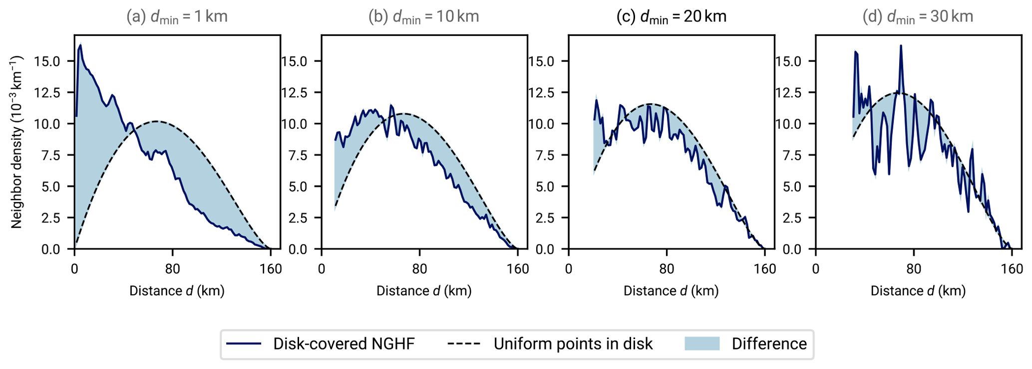
Figure 3 Spatial uniformity of heat flow measurements from the NGHF within disks with a radius of 80 km when varying the minimum inter-point distance d_min. Each graph shows neighbor distributions within disks with a radius of 80 km as a function of inter-neighbor distance d, that is, the number of neighboring data points at distance d from a data point within the disk, averaged over all points within the disks. The dashed lines show the expected distribution for a uniform distribution of points within the disks (derived in Appendix E). Deviations from the dashed lines indicate a non-uniform distribution of points within the disk. The solid blue lines show the empirical neighbor density obtained from disks with a radius of 80 km randomly distributed over Earth and selecting the NGHF data points within. The difference between the three panels lies in enforcing different minimum distances between NGHF data points. If two data points within a disk are closer together than the indicated d_min, a random one of them is removed. As d_min is increased, the neighbor distributions approach uniformity but fluctuations due to small number of remaining points within the disks increase. In this work, we choose d_min=20 km as a compromise between the two effects.

To mitigate the potential bias of spatial clustering, we enforce a minimum distance d_min between data points, using only one data point of pairs that violate this distance criterion. This realizes a more uniform spatial data distribution. In Fig. 3 we compare analytical expressions for the neighbor density under a uniform distribution (Appendix E) with the distance distribution between points of the filtered NGHF. The comparison leads us to choose a minimum distance of 20 km,

$$\begin{array}{}\text{(4)}& d_{\min }=\mathrm{20}\mathrm{km},\end{array}$$

between selected data points as a trade-off between uniform distribution and sufficient sampling.

Using only one data point of close pairs raises the question of which data point to choose. Ignoring the other data point ensures that the dependency between the data points is avoided, but it also results in loss of information about any spatially independent noise component. To retain the best of both worlds, we introduce a latent parameter that iterates all possible ways to select d_min-conforming subsets from the set of heat flow measurements in a region. Each value of the latent parameter therefore corresponds to a data set that we consider independent data within our model assumption and we can evaluate posterior distributions as described in Sect. 3.3.1 and 3.4. Figure 4 illustrates the generated subsets for a simple example.

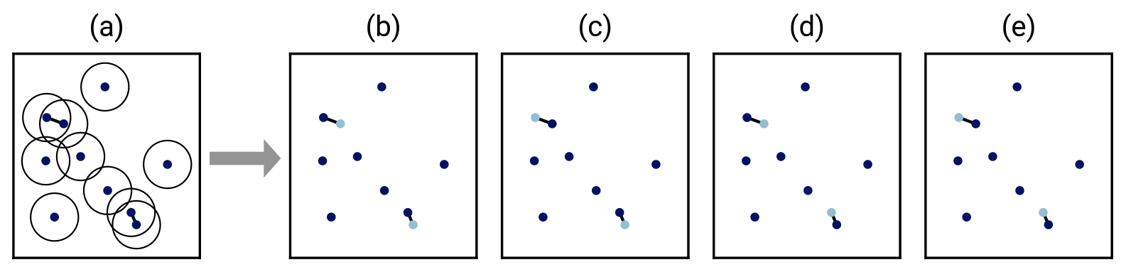
Figure 4 Selecting subsets of heat flow data when data point pairs violate the minimum-distance criterion. The circles in panel (a) indicate the radius d_min which is violated by the two marked point pairs. Panels (b) to (e) show the data point subsets that would be used in the handling of spatial data clusters: of each conflicting pair, a maximum of one data point is retained (fewer if the violations occur in clusters). In this simple scenario, panels (b) to (e) list all possible permutations. The REHEATFUNQ code approximates this permutation procedure stochastically for large sample sizes.

Choosing the parameter d_min, whether according to our value of 20 km or based on the data density within the ROI, is step 2 of the workflow listed in Appendix A.

3.3 Model description

3.3.1 A combined gamma model

The disaggregation of the heat flow measurements, Eq. (2), into different components is the basis for our model of regional aggregate heat flow. In particular, we consider the unknown heat flow q_u as a random variable. To yield useful results, this requires a model, that is, a probability distribution for q_u. In deriving a model for q_u, we make the following assumptions.

• I.

  The sum q_b+q_f is an independent and identically distributed (i.i.d.) gamma random variable.

• II.

  The sum q_s(x)+q_t(x) is an i.i.d. gamma-distributed random variable if x is the random variable that is derived from the spatial distribution of the heat flow data after applying the minimum-distance criterion (that is, successive point removal) in the right order.

• III.

  The right order follows the uniform distribution of permutations of the ordering of the heat flow data.

When both q_b+q_f and q_s(x)+q_t(x) are gamma distributed, the resulting sum q_u can be fairly well described by a gamma distribution (Covo and Elalouf, 2014). The sum is exactly gamma distributed when both q_b+q_f and q_s(x)+q_t(x) have the same scale parameter (Pitman, 1993). Hence, conditional on the right order, q_u is assumed to be gamma distributed and the likelihood of the remaining data points is the gamma likelihood. We can iterate the permutations of the ordering using a latent parameter, the permutation index $j\in \mathit{\{}\mathrm{1},\mathrm{\dots },N\mathrm{!}\mathit{\}}$. The probability of j is $P\left(j\right)=\mathrm{1}/N\mathrm{!}$. The full likelihood is then

$$\begin{array}{}\text{(5)}& \mathcal{L}(j,\mathit{\alpha },\mathit{\beta }|\mathit{\left\{}{q}_i\mathit{\right\}})=\mathit{\varphi }(\mathit{\alpha },\mathit{\beta }\left)P\right(j\left)\prod _{i\in \mathcal{I}\left(j\right)}\mathit{\gamma }\right(q_i|\mathit{\alpha },\mathit{\beta }),\end{array}$$

where ϕ(α,β) is the prior distribution of the gamma distribution; ℐ(j)={i}_j is the set of indices of data points in permutation j that are retained by the minimum-distance selection algorithm (see Sect. 3.2); and

$$\begin{array}{}\text{(6)}& \mathit{\gamma }\left(q_i\right|\mathit{\alpha },\mathit{\beta })={\displaystyle \frac{{\mathit{\beta }}^{\mathit{\alpha }}}{\mathrm{\Gamma }\left(\mathit{\alpha }\right)}}{q}_i^{\mathit{\alpha }-\mathrm{1}}\exp (-\mathit{\beta }{q}_i),\end{array}$$

with the gamma function Γ(α), is the gamma distribution for heat flow values q_i>0. Here we have used the parameterization of the gamma distribution with shape parameter α and rate parameter β. An alternative parameterization uses the scale parameter $\mathit{\theta }=\mathrm{1}/\mathit{\beta }$ instead.

The likelihood in Eq. (5) warrants two comments on its structure: first note that ℐ(j) always contains at least one index, the start of the permutation, due to the iterative resolution of the minimum-distance criterion. Secondly, if there is not a conflicting pair, ℐ(j) always contains all data indices and the j dimension trivially collapses to a uniform distribution. Otherwise, ℐ(j) can be a fairly complicated set.

Assumptions II and III are chosen to be peculiarly specific so as to yield a simple expression for the likelihood of the model. However, we can imagine a simple model of human data acquisition that is closely approximated by this likelihood. Imagine that a set of heat flow measurements is generated by the following process: initial drilling operations are distributed uniformly randomly over an area. Given that the level set of the underlying heat flow field is gamma distributed (or can be closely approximated by a gamma distribution), these initial drillings are gamma distributed as laid out in Sect. 3.1. Some of the initial wells turn out to be points of interest, for instance by identifying an oil or a geothermal field. Many of the following boreholes that lead to heat flow measurements would then cluster around these points of interest. This clustering, in turn, can lead to bias in the regional aggregate heat flow distributions due to the spatial correlation of q_s(x). If we were to know the spatial extent of the clusters (say, disks with a radius of d_min) and we assume that a priori each point within a cluster is equally likely to be the initial drilling, we could obtain the likelihood given in Eq. (5). In Appendix C we confirm that this simple physically inspired sampling mechanism leads to estimation biases, and we find that the minimum-distance sampling used in REHEATFUNQ is an effective counter measure.

Assumption I, the use of the gamma distribution, is motivated by the general right-skewed shape of global heat flow (see Fig. 1b), positivity of surface heat flow, and existence of a conjugate prior distribution (which greatly reduces the computational cost). Besides the aforementioned and rather subjective criteria and to have an objective evaluation, we performed goodness-of-fit tests (Sect. 4.1.3) that show that the gamma distribution is at least as competitive as other simple probability distributions on the positive real line in terms of describing the regional aggregate heat flow distributions.

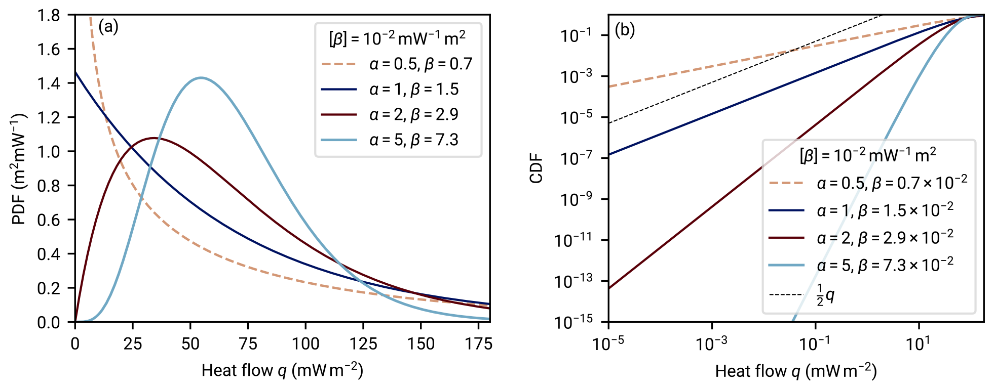
Figure 5 Gamma distribution as a model for regional aggregate heat flow. Panel (a) shows the probability density functions (PDFs) of four gamma distributions with a varying shape parameter α that all have the same mean 〈q〉=68.3 mW m⁻² (the mean of A quality data as estimated by Lucazeau, 2019). For α=1, the PDF is finite for q→0. For α>1, this limit is 0, and for α<1, the PDF has a singularity for q→0. Panel (b) shows the corresponding cumulative distribution functions (CDFs) with an emphasis on the asymptotics for small q values. A linear slope is plotted for comparison, corresponding to the growth of a uniform density with an increasing integration interval. The increased mass located in small q values in the case of α<1 becomes evident.

We restrict the parameter α to a minimum value of α_min=1 to prevent parameterizations with diverging densities at q→0 (see Fig. 5a). At α=1 the gamma distribution is an exponential distribution. For a smaller α, the density has a singularity at q=0. Illustratively, this causes the PDF to counter the effect of decreasing scale, and the mass decays only slowly on log scales in q.

Over the course of this paper, we will use the mean $\overline{q}$ and standard deviation σ_q of the gamma distribution. Parameterized by α and β, they are given as (Thomopoulos, 2018)

$$\begin{array}{}\text{(7)}& \overline{q}={\displaystyle \frac{\mathit{\alpha }}{\mathit{\beta }}}\text{ and }{\mathit{\sigma }}_q={\displaystyle \frac{\sqrt{\mathit{\alpha }}}{\mathit{\beta }}}.\end{array}$$

For frequentist inference of α and β, the maximum likelihood estimator will be used a couple of times in this work. A Newton–Raphson iteration with starting values given by Minka (2002) is used.

For a Bayesian analysis of both the regional aggregate heat flow distributions and the fault-generated heat flow anomaly, a prior distribution of the parameters α and β of the gamma distribution model is required – even if it is just the implicit improper uniform prior distribution. Using an informative prior distribution instead (see, e.g., Zondervan-Zwijnenburg et al., 2017) opens up the potential to include information from outside sources in a regional analysis. Because the number of measurements in regional heat flow analysis is generally small – the R=80 km RGRDCs created from NGHF A quality data typically contain 31 disks with an average of 11 points per disk – additional information can be valuable.

Ideally, we would like the prior distribution we use to be derived on physical grounds. We do not have any independent physical criteria for constructing the prior distribution, but our empirical gamma distribution model aims to capture the predominant physics underlying regional aggregate heat flow (we will later investigate how much so). Hence, a physical basis that can guide our prior distribution choice is the implied physics captured by our gamma distribution model. A prior distribution that is constructed from the gamma distribution is the empirically best choice to reflect these underlying physics. This role is generally fulfilled by conjugate prior distributions which arise from the associated probability density functions and whose hyperparameters represent aspects of the data that can become evident in the Bayesian updating.

For the gamma distribution, a conjugate prior distribution is given by Miller (1980), parameterized by the hyperparameters p, s, n, and ν. Its probability density in gamma distribution parameters (α,β) is

$$\begin{array}{}\text{(8)}& \mathit{\varphi }(\mathit{\alpha },\mathit{\beta }|p,s,n,\mathit{\nu })={\displaystyle \frac{{\mathit{\beta }}^{\mathit{\nu }\mathit{\alpha }-\mathrm{1}}{p}^{\mathit{\alpha }-\mathrm{1}}\exp (-s\mathit{\beta })}{\mathrm{\Gamma }\left(\mathit{\alpha }{)}^n\mathrm{\Phi }\right(p,s,n,\mathit{\nu })}}\end{array}$$

with gamma function Γ(α) and

$$\begin{array}{}\text{(9)}& \mathrm{\Phi }(p,s,n,\mathit{\nu })=\underset{a_{\min }}{\overset{\mathrm{\infty }}{\int }}\mathrm{d}\mathit{\alpha }{\displaystyle \frac{p^{\mathit{\alpha }-\mathrm{1}}\mathrm{\Gamma }\left(\mathit{\nu }\mathit{\alpha }\right)}{\mathrm{\Gamma }(\mathit{\alpha }{)}^n{s}^{\mathit{\nu }\mathit{\alpha }}}}.\end{array}$$

As in the previous section, we restrict the range of α from a_min=1 to infinity to exclude probability densities that diverge at q→0 and place considerable weight on negligible heat flow (say $q<{\mathrm{10}}^{-\mathrm{2}}$ mW m⁻²).

The conjugate prior distribution facilitates the computation of posterior distributions by means of Bayesian updating. The numerically expensive integrations over the parameter space of α and β that are involved in computing the posterior distribution are reduced to simple algebraic update rules of the conjugate prior distribution's parameters. Since numerical quadrature has the most computational cost in REHEATFUNQ and grows exponentially with the number of quadrature dimensions, reducing the set of quadratures to the computation of the normalization constant Φ of Eq. (9) significantly benefits the performance.

The Bayesian updating of the prior distribution of Eq. (8) given a sample $Q=\mathit{\{}{q}_i:\mathrm{1}\le i\le k\mathit{\}}$ of k heat flow values is (Miller, 1980)

$$\begin{array}{}\text{(10)}& \begin{array}{rl}& p^{*}=p\prod _i{q}_i,s^{*}=s+\sum _i{q}_i,\\ & n^{*}=n+k,{\mathit{\nu }}^{*}=\mathit{\nu }+k.\end{array}\end{array}$$

The posterior distribution of α and β is hence Φ of Eq. (8) with the starred parameters given above.

Given a prior distribution parameterization (p, s, n, ν), the probability density of heat flow within the region is the predictive distribution

$$\begin{array}{}\text{(11)}& \begin{array}{rl}\mathit{\psi }\left(q\right|p,s,n,\mathit{\nu })& =\underset{{\mathit{\alpha }}_{\min }}{\overset{\mathrm{\infty }}{\int }}\mathrm{d}\mathit{\alpha }\underset{\mathrm{0}}{\overset{\mathrm{\infty }}{\int }}\mathrm{d}\mathit{\beta }\mathit{\gamma }\left(q\right|\mathit{\alpha },\mathit{\beta }\left)\mathit{\varphi }\right(\mathit{\alpha },\mathit{\beta }|p,s,n,\mathit{\nu })\\ & ={\displaystyle \frac{\mathrm{\Phi }(pq,s+q,n+\mathrm{1},\mathit{\nu }+\mathrm{1})}{\mathrm{\Phi }(p,s,n,\mathit{\nu })}}.\end{array}\end{array}$$

Here, the final step utilizes the conjugate structure of the prior distribution.

This expression can be translated to the likelihood of Eq. (5) of the REHEATFUNQ model. The Bayesian update leads to the following proportionality:

$$\begin{array}{}\text{(12)}& \begin{array}{rl}& \mathit{\psi }\left(q\right|Q,p,s,n,\mathit{\nu })\\ & \sim \sum _{j=\mathrm{1}}^m\underset{{\mathit{\alpha }}_{\text{min}}}{\overset{\mathrm{\infty }}{\int }}\mathrm{d}\mathit{\alpha }\underset{\mathrm{0}}{\overset{\mathrm{\infty }}{\int }}\mathrm{d}\mathit{\beta }\mathit{\gamma }\left(q\right|\mathit{\alpha },\mathit{\beta }\left)\mathcal{L}\right(j,\mathit{\alpha },\mathit{\beta }\left|\mathit{\right\{}{q}_i\mathit{\left\}}\right).\end{array}\end{array}$$

After some algebra used in Eq. (11), this resolves to

$$\begin{array}{}\text{(13)}& \mathit{\psi }\left(q\right|Q,p,s,n,\mathit{\nu })={\displaystyle \frac{\sum _{j=\mathrm{1}}^m\mathrm{\Phi }(p_j^{*}q,s_j^{*}+q,n_j^{*}+\mathrm{1},{\mathit{\nu }}_j^{*}+\mathrm{1})}{\sum _{j=\mathrm{1}}^m\mathrm{\Phi }(p_j^{*},s_j^{*},n_j^{*},{\mathit{\nu }}_j^{*})}},\end{array}$$

where $p_j^{*}$, $s_j^{*}$, $n_j^{*}$, and ${\mathit{\nu }}_j^{*}$ are the parameters updated according to Eq. (10) with heat flow data set ℐ(j).

3.3.2 Minimum-surprise estimate

From a non-technical point of view, the purpose of the gamma conjugate prior distribution in the heat flow analysis is to transport universal information about surface heat flow on Earth while at the same time not significantly favoring any particular heat flow regime above other existing regimes. In other words, the prior distribution should penalize regions of the (α,β) parameter space that do not exist on Earth but should be rather uniform throughout the parts of (α,β) space that occur on Earth. The uniformity ensures that all regions on Earth are treated equally a priori in terms of heat flow, while the penalty adds universal information that can augment the aggregate heat flow data of each region.

In practice, a compromise between the uniform weighting of existing aggregate heat flow distributions and the penalizing of non-existent parameterizations needs to be found. Our choice in REHEATFUNQ is to put more weight onto the a priori uniformity of regional characteristics, that is, less bias. In parlance, we want to be minimally surprised by any of the distributions of the RGRDCs if we start from the prior distribution. One notion of the surprise contained in observed data when starting from a prior model is the Kullback–Leibler divergence (KLD) K from the prior distribution to the posterior distribution (Baldi, 2002):

$$\begin{array}{}\text{(14)}& {\displaystyle }K\left(p\right(\mathit{x}),\mathit{\varphi }(\mathit{x}\left)\right)=\underset{\mathcal{X}}{\int }{\mathrm{d}}^{n}xp\left(\mathit{x}\right)\ln {\displaystyle \frac{p\left(\mathit{x}\right)}{\mathit{\varphi }\left(\mathit{x}\right)}},\end{array}$$

where 𝒳 is the support of the parameters x. Baldi (2002) defines p(x) to be the prior distribution and ϕ(x) the posterior distribution given a set of observations.

The KLD is asymmetric, and Baldi and Itti (2010) note that the alternate order of probability distributions “may even be slightly preferable in settings where the `true' or `best' distribution is used as the first argument”. Here, we follow the alternate order and assign the gamma conjugate prior distribution to the role of ϕ(α,β). Furthermore, for the purpose of estimating the gamma conjugate prior distribution's parameters we consider the “uninformed” prior distribution (p=1, $s=n=\mathit{\nu }=\mathrm{0}$; Miller, 1980) updated to a regional heat flow data set using the update rules of Eq. (10) to be the “true” distribution p(α,β) within that region. In this order, minimizing the KLD of Eq. (14) is also known as the “principle of minimum discrimination information” (MDI hereafter; Kullback, 1959; Shore and Johnson, 1978), closely related to the “principle of maximum entropy” (Shore and Johnson, 1978).

Applying this estimator to a set of regional aggregate heat flow distributions leads us to the following cost function of the minimum surprise which we aim to minimize. We enumerate the regional aggregate heat flow distributions of the RGRDC by index i and the heat flow values within by index j with i-dependent range (Q_i={q_j}_i). We compute the updated parameters $p_i^{*}$, $s_i^{*}$, $n_i^{*}$, and ${\mathit{\nu }}_i^{*}$ starting from p=1, $s=n=\mathit{\nu }=\mathrm{0}$ for each Q_i. Then, the cost function reads

$$\begin{array}{}\text{(15)}& \begin{array}{rl}\textcolor{red}{}(p,s,n,\mathit{\nu }|\mathit{\left\{}{Q}_i\mathit{\right\}})=\underset{i}{max}& \left\{\underset{{\mathit{\alpha }}_{\min }}{\overset{\mathrm{\infty }}{\int }}\mathrm{d}\mathit{\alpha }\underset{\mathrm{0}}{\overset{\mathrm{\infty }}{\int }}\mathrm{d}\mathit{\beta }\mathit{\varphi }(\mathit{\alpha },\mathit{\beta }|p_i^{*},s_i^{*},n_i^{*},{\mathit{\nu }}_i^{*})\right.\\ & \left.\cdot \ln \left({\displaystyle \frac{\mathit{\varphi }(\mathit{\alpha },\mathit{\beta }|p_i^{*},s_i^{*},n_i^{*},{\mathit{\nu }}_i^{*})}{\mathit{\varphi }(\mathit{\alpha },\mathit{\beta }|p,s,n,\mathit{\nu })}}\right)\right\}.\end{array}\end{array}$$

On an algebraic level, the ith KLD term emphasizes scale differences between the prior distribution and the ith regional data-driven distribution in parts of the (α,β) space which the regional data favor, while other parts of the parameter space are less important. Taking the maximum over the distributions {i} ensures that across distributions, the regions in which probability mass is concentrated are equally accurately represented. Another advantageous property of the MDI estimator is that by taking into consideration the full probability mass, it can be better suited for small sample sizes than point estimators (e.g., Ekström, 2008).

An explicit expression for the numerical quadrature of Eq. (15) is given in Appendix D1.1. For the purpose of optimization, we substituted parameters

$$\begin{array}{}\text{(16)}& {\displaystyle }\mathit{x}=\left(\ln p,s,\ln ({\displaystyle \frac{n}{\mathit{\nu }}}-\mathrm{1}),\mathit{\nu }\right)\end{array}$$

with boundaries

$$\begin{array}{rl}& \ln p_{\min }\le x_{\mathrm{0}}\le \ln p_{\max },s_{\min }\le x_{\mathrm{1}}\le s_{\max },\\ & \ln \left(\mathtt{nv}\mathtt{\_}\mathrm{s}\mathtt{urplus}\mathtt{\_}\mathtt{min}\right)\le x_{\mathrm{2}}\le \ln \left(\mathtt{nv}\mathtt{\_}\mathtt{surplus}\mathtt{\_}\mathtt{max}\right),\\ & {\mathit{\nu }}_{\min }\le x_{\mathrm{3}}\le {\mathit{\nu }}_{\max }.\end{array}$$

With adjustable parameters

$$\begin{array}{rl}& \mathrm{0}<p_{\min }<p_{\max },\mathrm{0}<s_{\min }<s_{\max },\mathrm{0}<{\mathit{\nu }}_{\min }<{\mathit{\nu }}_{\max },\text{and}\\ & \mathrm{0}\le \mathtt{nv}\mathtt{\_}\mathtt{surplus}\mathtt{\_}\mathtt{min}\le \mathtt{nv}\mathtt{\_}\mathtt{surplus}\mathtt{\_}\mathtt{max},\end{array}$$

this substitution ensures that the parameter bounds in p, s, n, and ν are adhered to. Choosing to optimize the logarithm of $\frac{n}{\mathit{\nu }}-\mathrm{1}$ has shown itself to lead to a gracious convergence to the n=ν limiting case, and ln p is the standard expression of the p parameter in the numerical back end (see Appendix D).

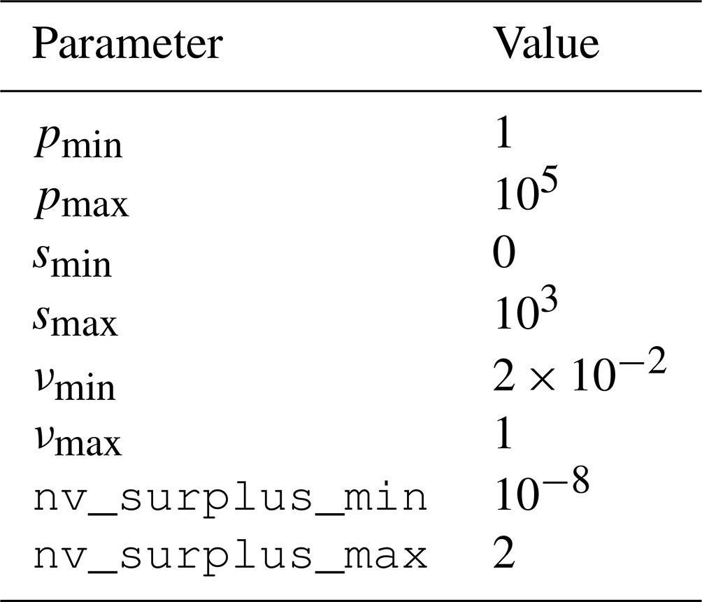
Before the global optimization of p, s, n, and ν, it is helpful to determine some a priori bounds on the parameters. One observation is that the minimum-surprise estimate (MSE) should not introduce a strong bias to the regional results. Miller (1980) noted that the parameterization in which the updated posterior distribution parameters are dependent on the data only is the “uninformed” prior distribution p=1, $s=n=\mathit{\nu }=\mathrm{0}$. This line of thought leads to heuristic bounds on the parameters for the MSE. The posterior distribution update rule for n and ν is an increment by the data count. Hence, the prior distribution $\widehat{n}$ and $\widehat{\mathit{\nu }}$ should be smaller than or close to 1 for our desired MSE if we expect less than one data point of “information”. For p the update rule is a product with each heat flow value q_i, and for s it is the sum with q_i. Hence, $\widehat{p}$ is expected not to be larger than 250^k, with, say, k∼1 and $\widehat{s}$ not larger than 250k. We have chosen conservative bounds based on these estimates and use the parameter bounds shown in Table 1.

Table 1 Parameter bounds used in the minimum-surprise estimate optimization.

To perform a global optimization of Eq. (15), we employ the simplicial homology global optimization (SHGO) algorithm implemented in SciPy (Endres et al., 2018; Virtanen et al., 2020). This algorithm starts with a uniform sampling of a compact multidimensional parameter space (we use the simplicial sampling strategy). The cost function is evaluated at the sample points, and a directed graph, approximating the cost function, is created by joining a Delaunay triangulation of the sample points with directions of cost increase. The key step of SHGO is then to determine local minimizers of this graph as starting points for further local optimization. The power of the algorithm is that under the condition that the cost function is Lipschitz continuous and the parameter space has been sampled sufficiently (whereby the directed graph is a sufficient representation of the cost function), the SHGO algorithm generates exactly one such starting point per local minimum. For the final iterative optimization of SHGO, we use the Nelder–Mead simplex algorithm (Nelder and Mead, 1965; Virtanen et al., 2020).

By manual investigation, we have found that setting the iteration parameter of SHGO to three, and using the boundaries previously defined, we obtain the optimum

$$\begin{array}{}\text{(17)}& \begin{array}{rl}& \widehat{p}=\mathrm{2.52202},\widehat{s}=\mathrm{15.3730},\widehat{n}=\mathrm{0.218477},\\ & \widehat{\mathit{\nu }}=\mathrm{0.218477}\end{array}\end{array}$$

with a final cost of  = 4.496. Two-dimensional slices of the local neighborhood of this optimum are displayed in Fig. S1 of the Supplement.

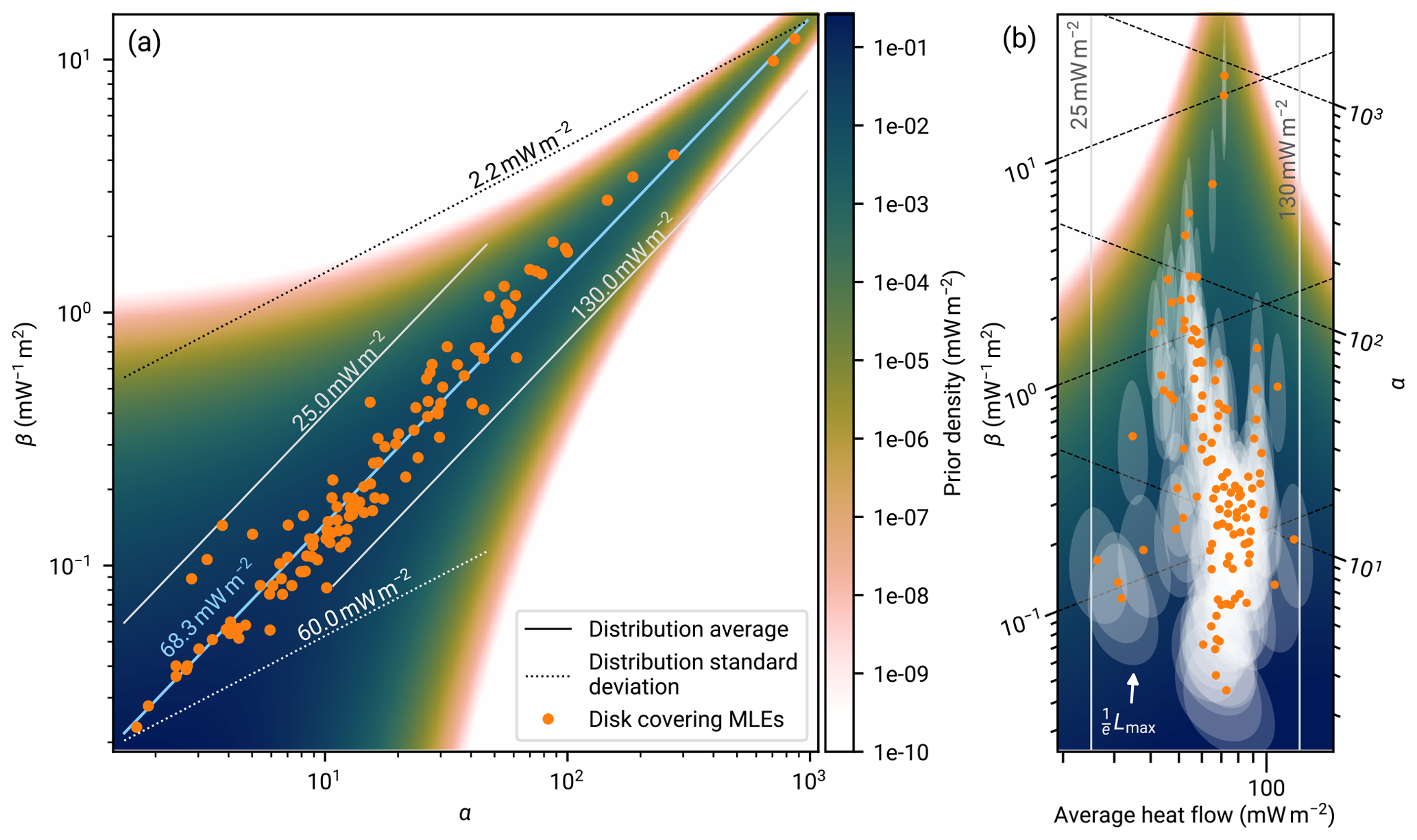
Figure 6 Analysis of the global heat flow database in mW m⁻² and parameter estimate of the gamma conjugate prior distribution of Eq. (8). Each dot marks the maximum likelihood estimate (MLE) of the gamma distribution parameters (α_i,β_i) for one of the randomly selected disk regions shown in Fig. 1 with the selection criterion of Sect. 2 applied. The solid lines mark parameter combinations of equal mean heat flow, and the dashed lines mark those with an equal standard deviation (after Thomopoulos, 2018). If the gamma distribution is assumed, global heat flow – split into disks with a radius of 80 km – can typically be described within a band of the parameter space given by a distribution average between 25 and 120 mW m⁻² and standard deviation of 3 to 60 mW m⁻². We capture this using the gamma conjugate prior distribution of Eq. (8) as the background color. Its parameters of $\widehat{p}=\mathrm{2.52202}$, $\widehat{s}=\mathrm{15.3730}$, $\widehat{n}=\mathrm{0.218477}$, and $\widehat{\mathit{\nu }}=\mathrm{0.218477}$ stem from the minimum-surprise estimate described in Sect. 3.3.2. (a) The global mean continental heat flow of 68.3 mW m⁻² is the estimate of Lucazeau (2019) from A quality data. Panel (b) shows a rotated and stretched section of the (α,β) parameter space such that the ordinate axis coincides with the average heat flow levels. The data are the same as in panel (a). Additionally we show, for each MLE, the region of the parameter space in which the corresponding likelihood is larger than $\mathrm{1}/e$ times its maximum. This illustrates the uncertainty in the parameter estimates.

The prior distribution ϕ(α,β) with our MSE parameters is shown in Fig. 6. There, we also show the maximum likelihood point estimates $(\widehat{\mathit{\alpha }},\widehat{\mathit{\beta }})$ for each of the regional aggregate heat flow distributions {Q_i} from the RGRDC used in the prior distribution parameter MSE. The shape of the prior distribution in Fig. 6a does not follow the scatter of the $(\widehat{\mathit{\alpha }},\widehat{\mathit{\beta }})$ estimates: while the $(\widehat{\mathit{\alpha }},\widehat{\mathit{\beta }})$ are, on logarithmic scales, within a constant range of a linear slope across scales, the prior distribution widens on log scales with a decreasing α and β. The picture changes when considering the estimate uncertainties which also increase with respect to the scatter of estimates for decreasing α and β (Fig. 6b). The prior distribution thus captures the effects of the gamma distribution parameters and the parameters' sensitivities for different α and β values.

With respect to heat flow, this implies that the average heat flow, as in Eq. (7), is fairly constant for any heat flow distribution. However, the sensitivity of the overall distribution relative to the distribution parameters – and consequently the uncertainty in the distribution estimates – changes with the distribution parameters. This sensitivity is relatively lower at smaller parameter values and vice versa. If a resulting distribution is less sensitive on the parameters, then in turn the uncertainties in estimating the parameters of such a distribution will increase, as even a large change in parameters will result only in a minor change of the resulting distribution. The prior distribution reflects this behavior.

Equation (11) for the posterior predictive distribution of regional heat flow can also be evaluated for the non-updated prior distribution. Figure 7 shows the PDF and the CDF for the prior distribution parameters of Eq. (17). The mode of the PDF is close to the average heat flow of A quality data within the NGHF, 68.3 mW m⁻² (Lucazeau, 2019). The prior predictive CDF follows the median CDF of the RGRDC samples fairly closely, with the exception of heat flow exceeding about 100 mW m⁻². The latter is linked to the heavy tail of the PDF, which aggregates about 4.3 % probability, while the data are cut at 250 mW m⁻².

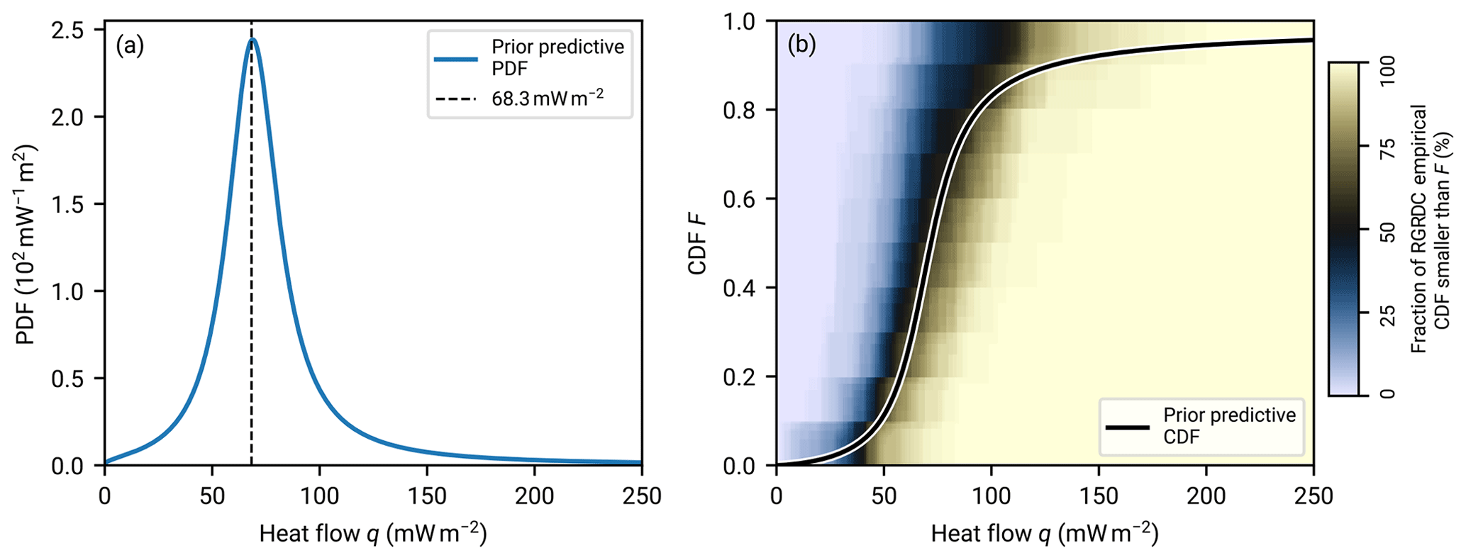
Figure 7 Prior predictive distribution for regional aggregate heat flow. The gamma conjugate prior distribution is parameterized as described in Eq. (17). Panel (a) shows the prior predictive PDF. The average value of A quality data from the NGHF (Lucazeau, 2019) is indicated. Panel (b) shows the prior predictive CDF. The background color shows, for each pixel in the (q,F) coordinates, the fraction of empirical cumulative distribution functions computed from the RGRDC heat flow samples at heat flow q which exceed F.

3.4 Bayesian inference of heat flow anomaly strength

We now turn to the quantification of the heat flow anomaly q_a(x). This signal q_a(x) is the surface heat flow signal due to a specific heat source that a researcher would like to investigate. It is implied that the surface heat flow field due to the heat source can be computed. In this article, we will use the heat flow signature of a vertical strike-slip fault with linearly increasing heat production with depth (Lachenbruch and Sass, 1980), but in principle REHEATFUNQ is agnostic to the type of surface heat flow to separate from the regional scatter. As noted in Sect. 3.1, the signal q_a can be separated from the regional undisturbed heat flow by means of Eq. (3) if the heat source is weak enough not to incite nonlinear convection.

In REHEATFUNQ, the heat flow anomaly signal q_a(x) is expressed by the total heat power P_H that characterizes the heat source and a location-dependent heat transfer function c(x) that models the surface heat flow per unit power that is caused by the heat source. This transfer function follows by solving the relevant heat transport equation. Given a power P_H and a function c(x), the heat flow anomaly contribution to the heat flow at measurement location x_i is thereby

$$\begin{array}{}\text{(18)}& {\displaystyle }{q}_{\mathrm{a}}\left(\mathit{x}\right)=P_{\mathrm{H}}c\left({\mathit{x}}_i\right)=P_{\mathrm{H}}{c}_i.\end{array}$$

Providing the coefficients c_i for each data point, by means of whichever solution technique to the heat transport equation available, is thereby the “application interface” of the REHEATFUNQ model for heat flow anomaly quantification. This is step 4 of the workflow listed in Appendix A. Note that while Eq. (18) requires the heat transport to be linear in P_H, in Appendix G we note a particular case of nonlinearity in the heat transport with respect to P_H that can still be addressed by REHEATFUNQ.

We can now combine the stochastic model for q_u and the deterministic model for q_a(P_H). Treating P_H as a model parameter, we perform Bayesian inference using the gamma distribution model for q_u. First, we transform the heat flow measurements by removing the influence of the heat flow signature:

$$\begin{array}{}\text{(19)}& {\displaystyle }{q}_i^{\prime }=q_i-P_{\mathrm{H}}{c}_i.\end{array}$$

The data $q_i^{\prime }$ are now data of the “unknown” or “undisturbed” heat flow, for which we use the gamma model γ(q_u) and its conjugate prior distribution.

Assuming the heat flow anomaly to be generated by a heat source implies the lower bound P_H≥0 (0 if the heat flow data are not at all compatible with the anomaly). From Eq. (19) an upper bound on P_H follows. Since we consider only positive heat flow,

$$\begin{array}{}\text{(20)}& {\displaystyle }{P}_{\mathrm{H}}^{\left(j\right)}\le \underset{i\in \mathcal{I}\left(j\right)}{min}\left\{{\displaystyle \frac{q_i}{c_i}}\right\}=:P_{\mathrm{H}}^{\mathrm{m},j}\end{array}$$

for any heat flow sample iterated by j. Outside of these bounds, we assume zero probability for this value of j. The global maximum P_H that can be reached across all j is

$$\begin{array}{}\text{(21)}& {\displaystyle }{P}_{\mathrm{H}}^{\max }:=\underset{\mathrm{1}\le j\le m}{max}\underset{i\in \mathcal{I}\left(j\right)}{min}\left\{{\displaystyle \frac{q_i}{c_i}}\right\}.\end{array}$$

Assuming a uniform prior distribution in P_H within these bounds, the full posterior distribution of the REHEATFUNQ anomaly quantification reads

$$\begin{array}{}\text{(22)}& \begin{array}{rl}& f(P_{\mathrm{H}},j,\mathit{\alpha },\mathit{\beta }|p,s,n,\mathit{\nu },\mathit{\left\{}\right(q_i,c_i\left)\mathit{\right\}})\\ & \sim \mathit{\varphi }(\mathit{\alpha },\mathit{\beta }|p,s,n,\mathit{\nu }\left)\prod _{i\in {\mathcal{I}}_j}\mathit{\gamma }\right(q_i-P_{\mathrm{H}}{c}_i|\mathit{\alpha },\mathit{\beta }).\end{array}\end{array}$$

To quantify the heat power P_H, REHEATFUNQ uses the marginal posterior distribution in P_H:

$$\begin{array}{}\text{(23)}& \begin{array}{rl}& f\left(P_{\mathrm{H}}\right|p,s,n,\mathit{\nu },\mathit{\left\{}\right(q_i,c_i\left)\mathit{\right\}})\\ & =\left\{\begin{array}{ll}{\displaystyle \frac{\mathrm{1}}{\mathcal{F}}}\sum _{j=\mathrm{1}}^m\underset{{\mathit{\alpha }}_{\min }}{\overset{\mathrm{\infty }}{\int }}\mathrm{d}\mathit{\alpha }\underset{\mathrm{0}}{\overset{\mathrm{\infty }}{\int }}\mathrm{d}\mathit{\beta }\mathit{\varphi }(\mathit{\alpha },\mathit{\beta })\prod _{i\in {\mathcal{I}}_j}\mathit{\gamma }\left(q_i^{\prime }\right|\mathit{\alpha },\mathit{\beta })& :P_{\mathrm{H}}\in [\mathrm{0},P_{\mathrm{H}}^{\max }]\\ \mathrm{0}& :\text{otherwise.}\end{array}\right.\end{array}\end{array}$$

In Appendix D2, we discuss how to compute the normalization constant ℱ.

If an upper bound on the heat power P_H is the aim of the investigation, the tail distribution (or complementary cumulative distribution function)

$$\begin{array}{}\text{(24)}& {\displaystyle }\overline{F}\left(P_{\mathrm{H}}\right)=\underset{P_{\mathrm{H}}}{\overset{\mathrm{\infty }}{\int }}\mathrm{d}Pf\left(P\right)\end{array}$$

can be used. It quantifies the probability with which the heat-generating power is P_H or larger.

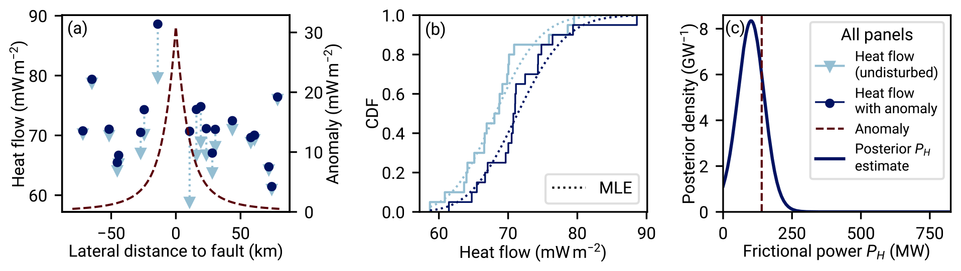
Figure 8 Sketch of the Bayesian analysis of the fault-generated heat flow anomaly strength. The analysis starts out in panel (a) with heat flow measurements (dots) in spatial relation to a known strike-slip fault. The heat flow measurements within the investigated region fluctuate, and they are distributed according to a probability distribution p(q). Here we use a gamma distribution with α=180 and β=2.6354319 mW⁻¹  m². These undisturbed fluctuations (triangles) are superposed by the fault-generated conductive heat flow anomaly (dashed line) to yield the measurements. Both the undisturbed data and the anomaly's strength are unknown to the researcher, but the anomaly can be modeled as a function of average frictional power P_H. Panel (b) shows the difference in aggregate cumulative distribution of the undisturbed heat flow and the data superposed by the anomaly. This is how REHEATFUNQ “sees” the data. Panel (c) shows the result of the REHEATFUNQ analysis. Our approach investigates the continuum of P_H. Each P_H corresponds to a heat flow anomaly of a different amplitude, which leads to different corrected data (from circles to triangles in panel a). The likelihood of the corrected data is evaluated against our proposed model of p(q), a gamma distribution, which leads to the posterior distribution of frictional power. In the case of this synthetic gamma-distributed data, the actual anomaly strength (vertical dashed line) is well assessed.

An illustration of the idea behind the approach in Eq. (23) is shown in Fig. 8. Panel a shows a sample of undisturbed heat flow q_u drawn from a gamma distribution. This heat flow is superposed with the conductive heat flow anomaly from a vertical strike-slip fault (Lachenbruch and Sass, 1980). The result is the sample of “measured” heat flow q. Undisturbed data at the center of the heat flow anomaly are collectively shifted to higher heat flow values, while those further away from the fault are barely influenced. Within the regional aggregate heat flow distribution, the most affected data will be shifted towards the tail. This distortion of the aggregate heat flow distribution is picked up by the likelihood with the result that correcting for the heat flow anomaly of the right power of P_H=140 MW (transforming the dots back to triangles in panel a) is more likely than no anomaly (P_H=0 W) in the right panel.

Figure 8 illustrates a core difficulty when identifying heat flow anomalies within noisy data of small sample sizes. The strength of the heat flow anomaly in this case is comparable to the intrinsic scatter of the regional aggregate heat flow distribution. This makes it difficult to identify the anomaly shape within the data. If the variance of the undisturbed heat flow is small compared to the actual magnitude of the anomaly, it becomes more and more feasible to visually identify the correct anomaly strength. Especially if the sample size is small, however, allowing for the occurrence of random fluctuations can significantly alter the interpretation of the data. The Bayesian analysis can capture all of this uncertainty in the posterior distribution of P_H, yielding a powerful analysis method.

3.4.1 Providing heat transport solutions

As outlined in Sect. 3.1, steady crustal heat transport can be conductive, advective, or convective. The REHEATFUNQ model can be applied as long as the surface heat flow at the data locations is linear in the frictional power P_H on the fault. The whole potentially complicated model of heat conduction from the fault to the data points can then be abstracted to the coefficients {c_i}. At present, the task of computing these coefficients for use in REHEATFUNQ lies generally with the user (step 4 of the workflow listed in Appendix A). Numerical methods such as the finite element, finite difference, or finite volume method as well as analytical solutions to simplified problem geometries can be used to determine {c_i} for a given problem by solving the heat transport equation of heat generated on the fault plane and dividing the surface heat flow at the data locations by the total frictional power P_H on the fault.

We illustrate this process using the single solution to the heat conduction equation that REHEATFUNQ presently implements: the surface heat flow anomaly generated by a vertical strike-slip fault. The solution stems from Lachenbruch and Sass (1980) and assumes a vertical fault in a homogeneous half-space medium. Furthermore, the fault is assumed to reach from depth d to the surface, and heat generation is assumed to increase linearly with depth up to a maximum Q^* at depth d. In the limit of infinite time, the stationary limit, the anomaly then reads

$$\begin{array}{}\text{(25)}& {\displaystyle }{q}_{\mathrm{a}}\left(x\right)={\displaystyle \frac{Q^{*}}{\mathit{\pi }}}\left(\mathrm{1}-{\displaystyle \frac{x}{d}}\arctan {\displaystyle \frac{d}{x}}\right)\text{ for }t\to \mathrm{\infty }.\end{array}$$

This shape of surface heat flow is shown in the sketch of Fig. 8. In REHEATFUNQ, the anomaly is implemented based on the surface fault trace. For each data point, the distance to the closest point on this fault segment string is computed and inserted as x into Eq. (25). For an infinite straight fault line in a homogeneous half space, this coincides exactly with the analytic solution. In real-world applications, the quality of this approximation depends on the straightness of the fault and its length compared to depth and data distance from the fault, as well as the dip of the fault – shallow-dipping faults lead to asymmetric heat flow instead.

The model of Eq. (25) leads to a heat production of $\overline{Q}d=Q^{*}d/\mathrm{2}$ per unit length of the fault. We can balance this with the total heat dissipation power P_H on a fault segment of length L within a region:

$$\begin{array}{}\text{(26)}& {\displaystyle }{Q}^{*}d=\mathrm{2}\overline{Q}d=\mathrm{2}{\displaystyle \frac{P_{\mathrm{H}}}{L}}.\end{array}$$

This finally leads to the following expression of the coefficients c_i as a function of distance to the surface fault trace:

$$\begin{array}{}\text{(27)}& {\displaystyle }{c}_i={\displaystyle \frac{q_{\mathrm{a}}\left(x_i\right)}{P_{\mathrm{H}}}}={\displaystyle \frac{\mathrm{2}}{\mathit{\pi }dL}}\left(\mathrm{1}-{\displaystyle \frac{x_i}{d}}\arctan {\displaystyle \frac{d}{x_i}}\right)\text{ for }t\to \mathrm{\infty }.\end{array}$$

To use the surface heat flow signature of other heat sources or to include advection, one would perform similar steps. First, the heat transport equation needs to be solved. An analytical solution like Eq. (25) will not often be available, so numerical techniques can be used to directly compute q_a(x_i) at the data locations for a given P_H. Then c_i, the input values to the posterior distribution of Eq. (23), can be computed by dividing the q_a(x_i) by P_H. The Python class AnomalyNearestNeighbor can then be used to specify the c_i for use in the REHEATFUNQ Python module.

3.4.2 Heat transport uncertainty

The model for heat transport will in general be uncertain. For instance, in Eq. (26) one might be able to narrow down the depth d only to within a certain range. Or one might have an alternative model based on a different geometry and perhaps another one that includes a small amount of groundwater advection. Such uncertainties in parameter values and model selection can be accounted for in REHEATFUNQ.

The interface to do so is via the coefficients c_i. The user can provide a set

$$\begin{array}{}\text{(28)}& {\displaystyle }\mathfrak{C}=\mathit{\left\{}\right(w_k,\mathit{\left\{}{c}_i{\mathit{\}}}_k\right):k=\mathrm{1},\mathrm{\dots },K\mathit{\}}\end{array}$$

of K solutions to the heat transport from source to heat flow data points. Each set {c_i}_k should contain a number N of coefficients c_i equal to the total number of heat flow data points before applying the d_min sampling (effectively this is a K×N matrix (c_ki)). The weights w_k quantify the probability that the user assigns to the heat transport solution k. In this way, k iterates a discretization of the N-dimensional probability distribution of the coefficients c_i.

Internally, REHEATFUNQ then uses a latent parameter $l\in \mathit{\{}\mathrm{1},\mathrm{\dots },m\times K\mathit{\}}$ to iterate the combinations of the latent parameter j with the index k (another latent parameter). Then, in all previous equations, the index j is replaced with k, the sets ℐ_j are replaced with the set ℐ_j(k) belonging to the index j that k iterates, and the coefficients c_i are replaced with c_ki. This effectively adds the k dimension to the REHEATFUNQ posterior distribution.

Since m×K is a possibly very large number – even j itself may be too large to iterate exhaustively and would hence be Monte Carlo sampled – only a user-provided maximum number of random indices l will be used in the sums.

4 Model validation and limitations

The previous methodology section described the idea behind considering regional aggregate heat flow as a random variable and set out straightforwardly to describe the REHEATFUNQ gamma model and its prior distribution parameter estimation. Yet, no physical basis has been provided for the choice of a gamma distribution besides a number of general properties that the gamma distribution, among others, fulfills. In this section, we provide a posteriori support for this choice.

In Sect. 4.1.1–4.1.3, the NGHF (Lucazeau, 2019) will be used to investigate whether the REHEATFUNQ gamma model is suitable for the description of real-world heat flow data. The analysis reveals a degree of misfit for which we investigate possible causes. Finally, we compare the gamma model to other two-parameter univariate probability distributions.

In Sect. 4.2 and its subsections, we analyze synthetic data, allowing us to leverage large sample sizes. We investigate how well REHEATFUNQ can quantify heat flow anomalies both if the regional aggregate heat flow were gamma distributed, that is, according to the model assumptions, and if the regional heat flow were to follow some strongly gamma-deviating mixture distributions found in the NGHF in Sect. 4.1.1. Furthermore, we investigate the impact of the prior distribution parameters on the anomaly quantification.

In Sect. 4.3 and its subsections, we discuss some physical limitations of the REHEATFUNQ model.

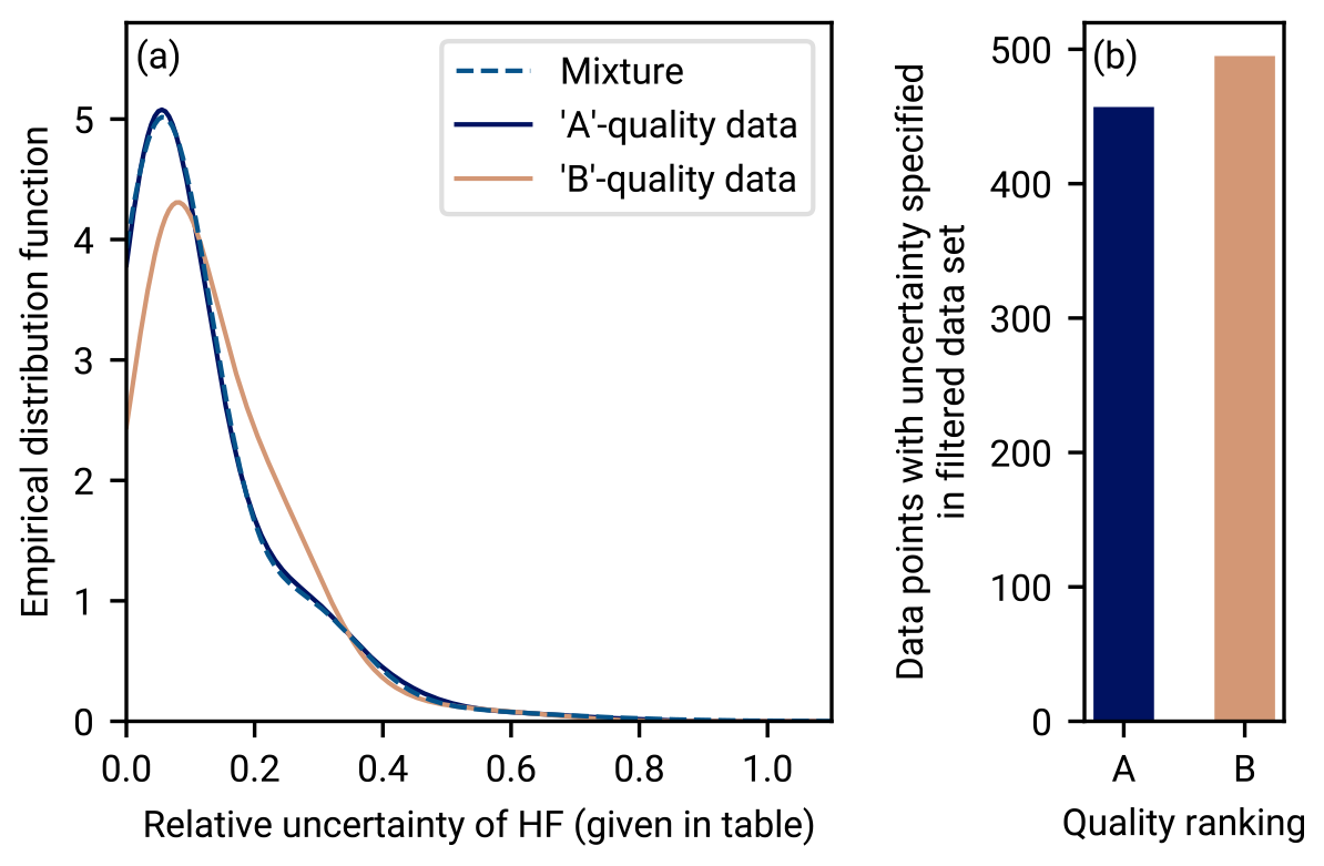
Figure 9 Distribution of relative error in the NGHF database for A and B quality data. We show only A and B quality data according to our data filtering described in Sect. 2.1. Panel (a) shows the distribution of relative uncertainty for data records of A and B quality, from the filtered NGHF database, for which an uncertainty is specified. The dashed line shows a mixture distribution of three normal distributions that approximates the relative error distribution of the A quality data. The parameters of the mixture are means $\mathit{\mu }=(\mathrm{0.055},\mathrm{0.272},\mathrm{0.36})$, standard deviations $\mathit{\sigma }=(\mathrm{0.08},\mathrm{0.09},\mathrm{0.24})$, and weights $\mathit{w}=(\mathrm{0.79},\mathrm{0.15},\mathrm{0.06})$. Panel (b) shows a histogram of the number of data records of A and B for which uncertainty is specified and which pass our data selection criteria.

4.1 Validation using real-world data

4.1.1 Goodness of fit: region size

Interpreting the regional heat flow as a stochastic, fluctuating background heat flow introduces a potential trade-off in the region size. On the one hand, considering heat flow data points across a larger area increases the number of heat flow measurements, which can increase the statistical significance of the analysis. In particular when investigating fault-generated heat flow anomalies, data points further away from the fault, say >20 km (see Fig. 8), are less influenced by the fault heat flow and can hence better quantify the background heat flow that is not disturbed by the heat flow anomaly. On the other hand, increasing the region size makes the analysis more susceptible to capturing large-scale spatial trends. These trends may introduce correlations or clustering between the data points which are not captured by the stochastic model. Conversely, using smaller region extents will improve the quality of approximating large-scale spatial trends as uniform. We will now set out to find a compromise between these effects by finding a region size in which we can hope to apply the gamma model for regional aggregate heat flow distributions.

Our goodness-of-fit analysis by region size region is based on RGRDCs (see Appendix B). For each regional aggregate heat flow distribution, we investigate how well the sample can be described by the gamma distribution. Control over the radius R allows us to investigate the fit over various spatial scales.

We performed tests based on the empirical distribution function (EDF tests; Stephens, 1986) to investigate the goodness of fit. We have used the Kolmogorov–Smirnov (KS) and Anderson–Darling (AD) test statistics, and we have applied them for the case that both parameters α and β are unknown (“case 3” of Stephens, 1986). We calculated critical tables for the test statistics covering the sample sizes and maximum likelihood estimate shape parameters $\stackrel{\mathrm{̃}}{\mathit{\alpha }}$ that we encountered in the RGRDCs since the tables are independent of β as a scale parameter (David and Johnson, 1948). The critical tables yield the values for both test statistics that are exceeded at a certain rate if the data stem from a gamma distribution (we chose a 5 % rejection rate). This rejection rate means that if N samples of size M are drawn from a gamma distribution with shape α, the KS test statistic exceeds the value read from the KS critical table for that M and α in 5 % of the samples. The same holds for the AD statistic and the AD critical table. Hence if regional aggregate heat flow distributions were gamma distributed, we would expect 5 % of disks to be rejected by the tests. Higher rejection rates (number of rejected samples $/$ number of samples) indicate that they are not gamma distributed.

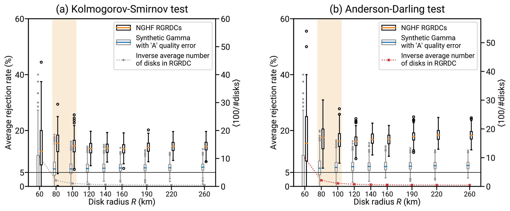
Figure 10 Investigating the fit of various probability distributions to the NGHF (Lucazeau, 2019) at different spatial scales. Both sides analyze the same data sets using goodness-of-fit (GOF) tests for the gamma distribution (e.g., Stephens, 1986). First, we analyze RGRDCs of the NGHF data set (defined in Appendix B). For each disk of a global covering, a GOF test is performed for the distribution of heat flow within. The average rejection rate is the fraction of disks within a covering for which the gamma hypothesis is rejected at the α = 5 % level. For sufficiently large samples from a gamma distribution, this rate would converge to 5 %. The black box plots show, for each indicated R, the distribution of these rejection rates over 200 generated coverings. The gray box plots show the same distribution for synthetic gamma-distributed global coverings (details in Appendix B1). Known processes affecting the used part of the NGHF data set (250 mW m⁻² threshold, discretization, and typical uncertainty) have been simulated. The box plots show the median (colored bar), quartiles (extent of the box), up to 1.5 times the interquartile range (whiskers), and outliers thereof. The box plot shows a separation of the two rejection rate distributions, indicating that there are patterns in the real heat flow data that cannot be explained by a gamma distribution and uncertainty. As R decreases, the discrepancy decreases as well until at R≲80 km, the R disks contain too few data points to resolve the average rejection rate properly (illustrated by the dashed line showing the average of 100 divided by the number of disks in a covering).

Figure 10 shows the results of the goodness-of-fit analysis. Two R-dependent effects can be observed in Fig. 10: at a small R of <80 km, the scatter of small sample sizes becomes dominant. There are just too few regions remaining. For an increasing R, the rate of rejecting the gamma distribution hypothesis increases slightly.

A striking observation is that for all of the region sizes, the rejection rate is larger than 5 % (centered at about 15 %) and the fluctuations in rejection rates across different RGRDCs do not alter that conclusion. Regional aggregate heat flow is not generally gamma distributed.

This deviation is not due to known heat flow data uncertainty. To test whether the heat flow data uncertainty might be the cause of the elevated rate of rejections, we have performed a synthetic analysis using synthetic RGRDCs generated by the algorithm in Appendix B1. After generating gamma-distributed random values similar to RGRDC data, relative error following the uncertainty distribution of A and B data (shown in Fig. 9) is added to the data. The resulting rejection rates show a spread similar to that of the NGHF data, but the bias is small (the median of the rejection rates across synthetic RGRDCs never exceeds ∼8 %). Consequently, unbiased random error as specified for the heat flow data within the NGHF is not sufficient to describe the ∼15 % rejection rate of the gamma model.

The impact that this imperfect model of regional aggregate heat flow has on the accuracy of the results is not immediately clear. On the one hand, using a wrong model to analyze the data suggests a detrimental impact on the accuracy. On the other hand, if the model is close enough, the method might be accurate up to a desirable precision. Later in Sect. 4.2.2 we investigate, using synthetic data, how well REHEATFUNQ can quantify heat flow anomalies when regional aggregate heat flow data is decidedly non-gamma distributed.

Before these synthetic investigations, the following sections investigate potential causes for the deviation from a gamma distribution in Sect. 4.1.2 and test whether other parsimonious models for the regional aggregate heat flow distribution perform better than the gamma distribution on RGRDCs of the NGHF data set in Sect. 4.1.3.

4.1.2 Goodness of fit: the level of misfit from mixture models

Following the observation that the gamma distribution is not a general description of regional aggregate heat flow distributions, we investigate potential causes for this misfit and how large the deviation from a gamma distribution has to be to produce the ∼15 % rejection rates of the previous section.

We find that the mismatch could be explained by mixture distributions. Figure 11 shows the same RGRDCs Anderson–Darling rejection rate as Fig. 10 and additionally the rejection rate computed for two mixtures of two gamma distributions each. The two mixture distributions are synthetic but cover the range of typical heat flow values, and the samples drawn from them have the sample size distribution as the RGRDCs. One distribution (“mix 0”) has less overlap between the two peaks than the other and leads to large rejection rates of ∼80 %. The other, “mix 1”, has more overlap between the peaks, and they are more equally weighted. This mixture model matches the observed rejection rates across the NGHF data RGRDCs very closely. Similar mixture models could hence be a possible cause for the observed rejection rates across the NGHF if the heat flow were indeed gamma distributed.

The mixture distribution can arise in the real heat flow data if the disk intersects a boundary between two regions of different heat flow characteristics. Since radiogenic heat production in the relevant upper crust can vary on the kilometer scale (Jaupart and Mareschal, 2005), such an occurrence seems plausible. The occurrence of a boundary intersection mixture might be frequent and with a smaller difference between the modes (corresponding to mix 1), or it might be infrequent but with a larger inter-mode distance (dashed line in Fig. 11). Both cases are compatible with the statistics observed in the NGHF data RGRDCs.

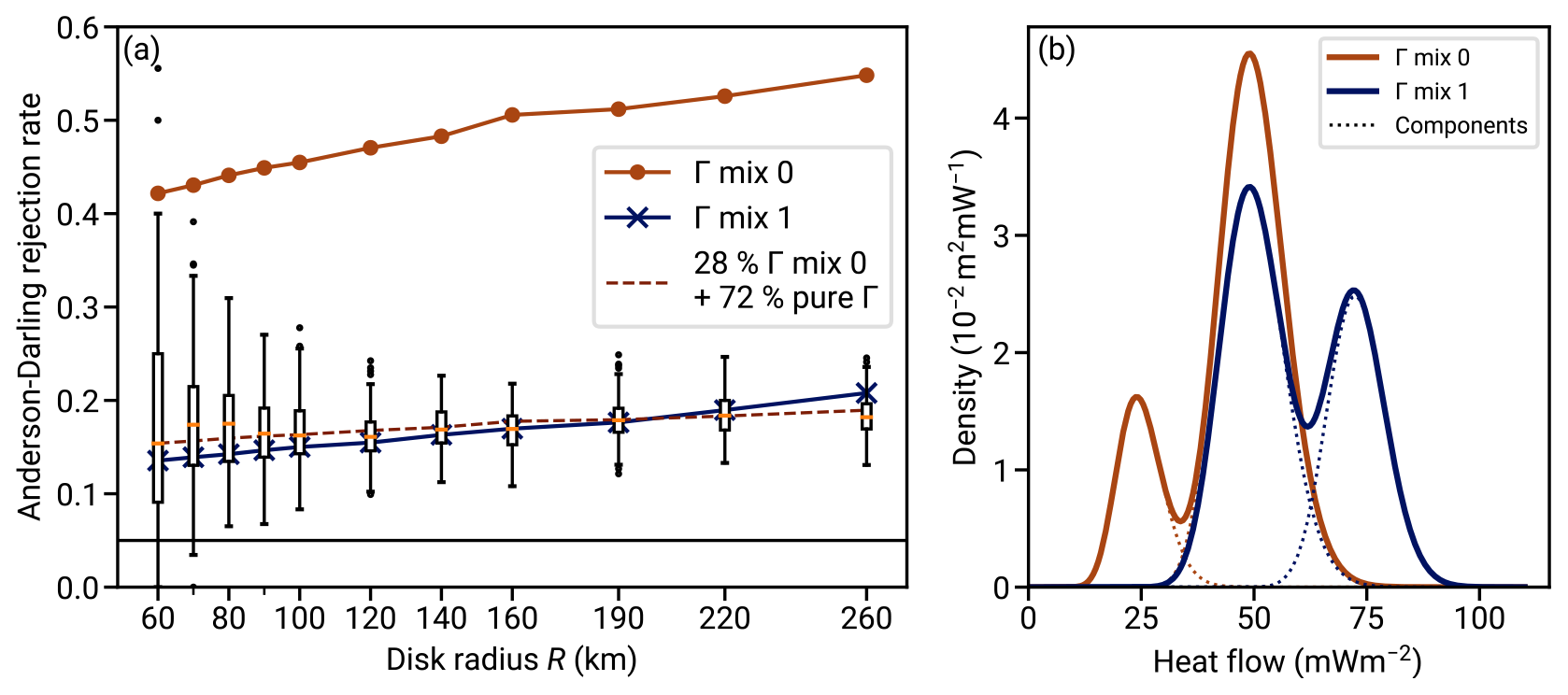
Figure 11 Exploring the misfit between the gamma distribution model of regional heat flow and the NGHF data. (a) Box plots show the fraction of heat flow distributions from RGRDCs of the NGHF database for which the gamma distribution hypothesis is rejected at the 5 % level (same data as Fig. 10b). The solid lines with dots show the same fraction of rejections computed for two sets of 10 000 samples each, drawn from the two gamma mixture models shown in panel (b) (colors corresponding). Each sample from the mixture distributions has its size drawn from an NGHF RGRDC of the corresponding R, replicating the sample size structure derived from the NGHF. The dashed line in the left plot shows the case if 72 % of the samples were gamma distributed (5 % rejection rate, horizontal black line), while 28 % of the samples were draft from mixture model 0. (b) The dotted lines indicate the two gamma distributions comprising each mixture. The parameters are w₀=0.2, k₀=25, θ₀=1 mW m⁻², k₁=50, and θ₁=1 mW m⁻² for Γ₀ (where w₀ is the weight of the zero-index component) and w₀=0.4, k₀=128, θ₀=0.57 mW m⁻², k₁=50, and θ₁ = 1 mW m⁻² for Γ₁.

The match with the observed rejection rates is not conclusive evidence that the heat flow data within the regions follow gamma mixture distributions. It is likely that many different distributions could be constructed that lead to similar rejection rates. However the match is a good indication of how large the deviation between the underlying distribution and the simple gamma model is. Somewhere between “gamma mix 0” and “gamma mix 1” lies a critical point in terms of mode separation beyond which the distribution would depart further from a gamma distribution than what is observed in the NGHF data RGRDCs.

At this point, we can summarize that heat flow in disks with a radius of 60 to 260 km is not generally gamma distributed and this is not an artifact of data processing or uncertainty. Mixtures of gamma distributions within the disks, for instance representing variation on smaller scales below the smallest radius we can investigate, could explain the mismatch. Moreover, the mixtures indicate the level of mismatch that would lead to the statistics observed in the real heat flow data.

We proceed in Sect. 4.1.3 by investigating whether other two-parameter univariate probability distributions perform better in describing the real-world regional aggregate heat flow distributions. Later in Sect. 4.2.2, we will investigate the impact that the misfit of the gamma model has on the quantification of heat flow anomalies. This will drive the model despite the mismatch to observed data until a physics-derived alternative becomes available.

4.1.3 Comparison with other distributions

We compare the performance of the gamma distribution with a number of common probability distributions. This aims to investigate whether the mismatch can be resolved by choosing another simple probability distribution or whether the gamma distribution performs well in terms of a simple model.

The comparison is performed at the transition point between an insufficient sample size, as the radius decreases, and increasing misfit, as the radius increases. The radius is 80 km. Even though the global heat flow database of Lucazeau (2019) is large, the number of samples within a disk of R=80 km is rather small at a 20 km minimum distance between the data points (typically 11). Therefore, we focus our analysis on two-parameter models.

We generate samples from the NGHF using the RGRDCs described in Appendix B. To each disk's sample, we fit probability distribution candidates using maximum likelihood estimators and compute the Bayesian information criterion (BIC; Kass and Raftery, 1995). The probability distribution with the smallest BIC is the most favorable for describing the subset, and the absolute difference ΔBIC to the BIC of the other distributions indicates how significant the improvement is. In our particular case, ΔBIC depends only on differences in the likelihood since all investigated distributions are two-parametric. We repeat the process 1000 times to prevent a specific random regional heat flow sample selection skewing the results (see Figs. S9–S11 in the Supplement for a convergence analysis).

Due to the right-skewed shape of the global distribution (see Fig. 1b), we test a range of right-skewed distributions on the positive real numbers: the Fréchet, gamma, inverse gamma, log-logistic, Nakagami's m, shifted Gompertz, log-normal, and two-parameter Weibull distribution (Bemmaor, 1994; Leemis and McQueston, 2008; Kroese et al., 2011; Nakagami, 1960). The global distribution does not have to be representative of the regional distributions, however. Since the global distribution is a mixture of the regional distributions, only the weighted sum of the regional distributions needs to have the right-skewed shape. Therefore, we additionally test the normal distribution (e.g., used by Lucazeau, 2019).

In Fig. 12c, the results of the analysis are visualized using the rate of BIC selection, that is, the fraction of regional heat flow samples for which the hypothesized distribution has the lowest BIC. Furthermore in panel a, the distribution of ΔBIC to the second-lowest scoring distribution is shown for the samples in which each distribution is selected, and in panel b the distribution of (negative) ΔBIC to the selected distribution is shown for the samples in which each distribution is not selected. The Weibull distribution has the highest selection rate, followed by the Fréchet distribution. Combined, they account for roughly 60 % of all selections. Together with the normal distribution and one outlier of the log-logistic distribution, they are the only distributions with occurrences of ΔBIC > 2, which might be considered “positive evidence” (Kass and Raftery, 1995, p. 777). However, these ΔBIC > 2 instances occur only in less than 4.4 % of the total subsets for each of the three distributions. Therefore, no distribution is unanimously best at describing the regional heat flow.

The ΔBIC for regions in which a distribution is not selected leads to a different selection criterion: if a distribution is not the best-scoring distribution, how much worse than the best is it? These differences are generally more pronounced than the differences in the best to the second-best fitting model. Especially the Fréchet and inverse gamma distribution perform much (strong evidence at ΔBIC > 6, Kass and Raftery, 1995, p. 777) worse than the better-fitting distributions in more than 50 % of the cases in which they are not selected. The generally least worst performing models are the gamma, log-logistic, normal, Nakagami, and Weibull distribution. Their negative ΔBIC distributions have only minor differences, and different ones perform better depending on the quantile of the negative ΔBIC investigated.

To conclude, the gamma distribution is among the best-performing distributions in terms of a consistently good description of the data. There are no significant differences between the distributions in terms of fitting the data that would favor any of the other distributions over the gamma distribution. Up until the typical shape of the regional aggregate heat flow distribution is derived from physical principles, the choice among the set of the best-performing distributions remains a modeling decision. Here, the gamma distribution is the only distribution of the best-performing set that fulfills all three of the following criteria: (1) it is defined by positive support; (2) it has a conjugate prior distribution for enabling costly computations; and (3) it is right-skewed, like the global heat flow distribution, for all parameter combinations. We hence choose the gamma distribution within REHEATFUNQ.

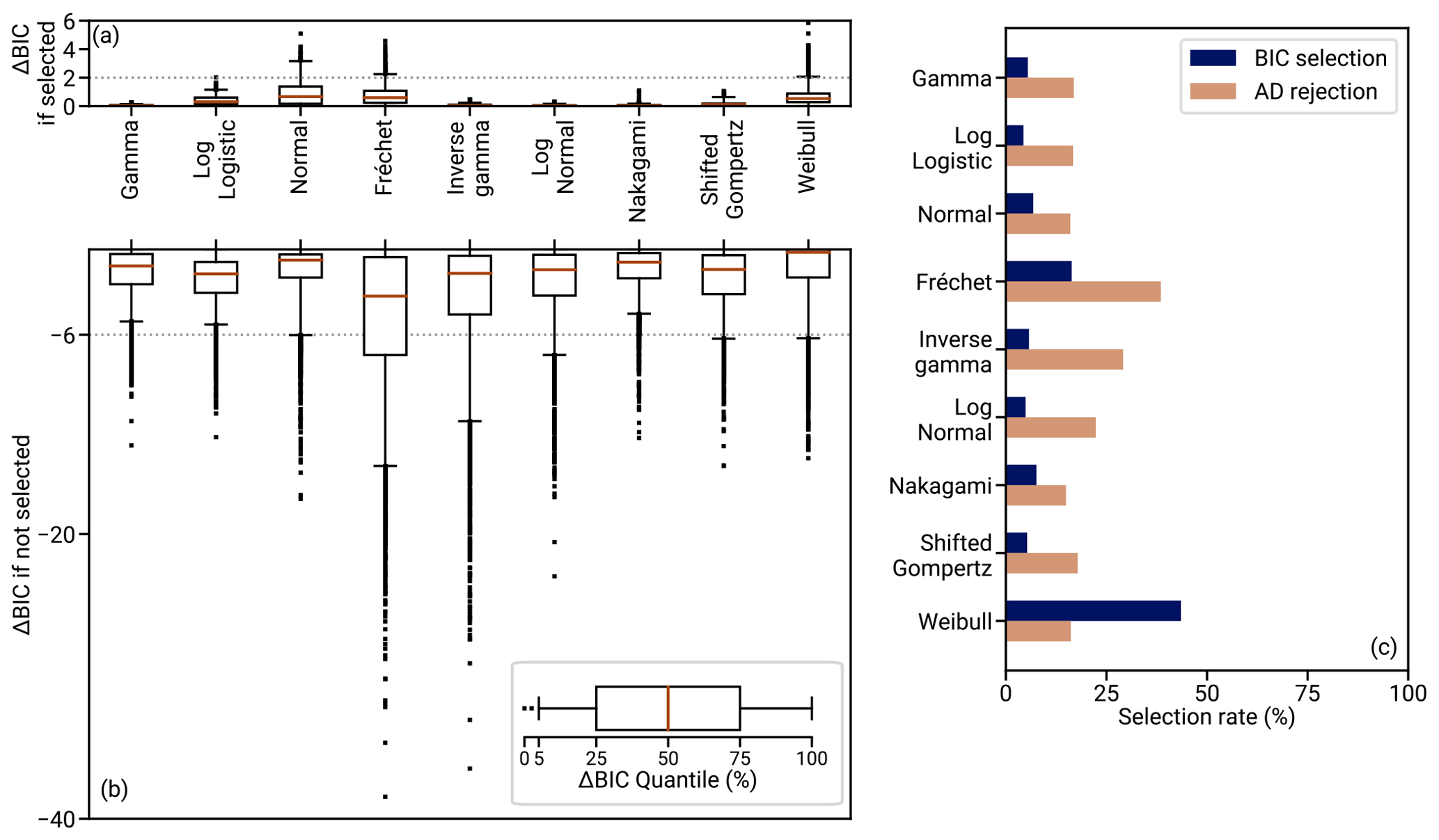
Figure 12 Selection rates, as well as their significance, of different two-parameter probability distributions for modeling regional heat flow distributions for global coverings of circles with a radius of 80 km. (c) Given an RGRDC (described in Appendix B), the selection rate denotes the fraction of these regions for which the indicated distribution has the lowest BIC. (a) The box plots show the distribution of ΔBIC conditional to the respective distribution being selected (that is, each time it has the lowest BIC). ΔBIC is then computed as the distance of this lowest BIC value to the second-lowest BIC value. In other words, it quantifies how much better than the best competition the distribution performs if selected. Panel (b) shows in similar box plots the distribution of ΔBIC to the lowest scoring distribution among the regional heat flow samples in which the indicated distribution is not selected. In other words, the bottom panel shows how much worse than the best-fitting distribution each distribution is if it is not the best (values closer to 0 are better). The data of all three panels are aggregated from 100 random global coverings.

4.2 Validation using synthetic data

In this section we analyze the performance of the complete anomaly-testing model described in Sect. 3.4 using synthetic data, that is, computer-generated samples $\mathit{\left\{}\right(x,y,q{)}_i\mathit{\}}$ of surface heat flow. The purpose of this test is to investigate the impact of the conjugate prior distribution, the model's correct identification of synthetic anomalies, and the impact that the deviation of real-world data from the assumed gamma distribution could have on the model's performance.

In the following sections, a number N of artificial heat flow values within a disk with a radius of 80 km are generated following a variety of distributions. To investigate the impact of the sample size and potential convergence, N is varied in the synthetic experiments. We note that in these tests, the minimum distance of 20 km between data points is not enforced. As a consequence, we can also investigate data set sizes larger than 64 samples, which might be close to the densest point packing within a circle with a ratio of the minimum distance to the radius of 0.25 (Graham et al., 1998), that is, the maximum our minimum-distance criterion allows.

The minimum data set size we investigate is 10, corresponding to a density of $\mathrm{5.0}\times {\mathrm{10}}^{-\mathrm{4}}$ km⁻². The densest packing of 64 data points corresponds to a density of $\mathrm{3.2}\times {\mathrm{10}}^{-\mathrm{3}}$ km⁻², and the maximum sample size we investigate, 100, corresponds to a density of $\mathrm{5}\times {\mathrm{10}}^{-\mathrm{3}}$ km⁻² inside a disk with a radius of 80 km. When enforcing the 20 km minimum distance, 100 samples would correspond to the most densely packed circle with a radius of ≃100 km (López and Beasley, 2011, Table 4, result minus 1) and again a density of $\mathrm{3.2}\times {\mathrm{10}}^{-\mathrm{3}}$ km⁻².

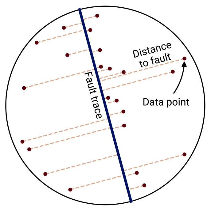
Figure 13 Configuration of the synthetic heat flow data and fault in the synthetic method tests (Sect. 4.2 and subsections). The configuration is chosen to reflect both the random global R-disk coverings used in Sect. 4.1.1 and the heat flow anomaly of the San Andreas fault used in Sect. 5. The regions are disks with a radius of 80 km in which the locations of synthetic heat flow measurements (dots) are distributed according to a uniform probability density. A straight fault (thick line) intersects the disk through its center. The dashed lines show the distances x of the heat flow data from the fault trace, which are used to determine the anomaly strength c_i as a function of frictional power P_H dissipated on the fault segment. The anomaly shape is in accordance with Eq. (25), following Lachenbruch and Sass (1980), which is displayed in Fig. 8.

4.2.1 Impact of the conjugate prior distribution

In this first of two tests, we investigate how well the method is able to identify synthetic anomalies that have been superimposed on artificial gamma-distributed heat flow values. Specifically, this aims to investigate the impact of the prior distribution for small data sets. To this end, we compare our choice of prior distribution parameters, in Eq. (17), with an (improper) uninformed prior distribution of p=1, $s=n=\mathit{\nu }=\mathrm{0}$, whose posterior parameters are determined solely by the data.

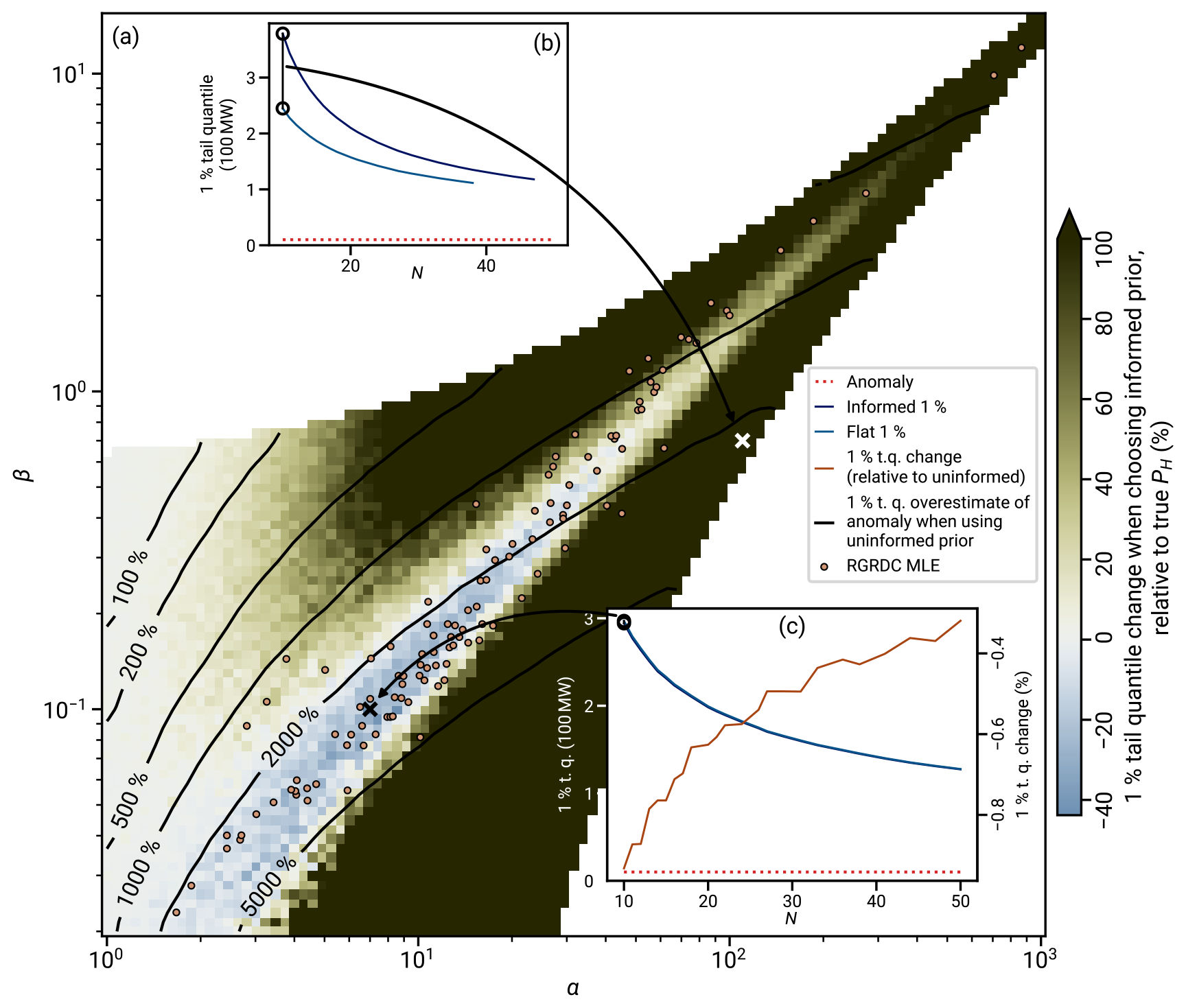
Figure 14 Performance of the anomaly testing with the posterior distribution of Eq. (23) for synthetic data. Heat flow data (N=10) have been generated from gamma distributions with α and β according to the position within the two-dimensional parameter space, and each data point has been assigned a lateral distance between -80 and 80 km from a vertical fault segment of 14 km depth and 160 km length. Afterwards, an anomaly with 10 MW according to the model of Eq. (25) has been added to the data, and quantiles of the posterior tail distribution (23) have been computed. This background color has been computed from 1000 such synthetic data sets. It shows the median of the relative difference between the 1 % tail quantiles (t.q.) computed from the informed (17) and a flat (p=1, $s=n=\mathit{\nu }=\mathrm{0}$) prior distribution. A value below 0 (light-blue color) indicates that the informed prior distribution results in a lower 1 % tail quantile, that is, provides stronger constraints. Such a point in the (α,β) parameter space is shown in inlay (c), corresponding to the black cross, where we have performed the analysis for 100 000 synthetic data sets and different N values. A positive background color value in the (α,β) space indicates that the flat prior distribution imposes a tighter constraint on the anomaly. Such a data point is shown in inlay (b), corresponding to the white cross. In all points of the parameter space shown here, the median 1 % percentile of both prior distributions is larger than the actual anomaly; i.e. no underprediction of the anomaly strength occurs. Top left and bottom right white parts of the parameter space are unlikely volumes of the prior distribution (17) and have not been investigated.

In Fig. 14, the performance of the model is evaluated on synthetic data generated from gamma distributions and superposed with a synthetic anomaly of a vertical fault following Lachenbruch and Sass (1980). The anomaly of Eq. (25) is computed for a power of 10 MW and the spatial configuration shown in Fig. 13. Both using the prior distribution with parameters of Eq. (17) and a flat prior distribution, the marginal posterior distribution imposes correct bounds on the anomaly strength with increasing precision as the sample size increases.

The difference between the flat and the informed prior distribution is most pronounced at small sample sizes and standard deviations. There, the flat prior distribution places a considerably tighter constraint on the anomaly strength. At larger standard deviations, a region emerges in which this relation is reversed and the informed prior distribution leads to stricter constraints, albeit considerably less so (less than 10 % improvement on the 1 % tail quantile bound). This region coincides in part with the isolines of the prior density (see Fig. 6). Since the region lies in a part of the (α,β) space with a larger standard deviation, improvements in this area can be helpful.

All in all, the impact of the informed prior distribution is ambiguous. In a part of the (α,β) space that is densely covered by modes of the RGRDC likelihoods and which is hence likely to cover the regional aggregate heat flow distribution of a heat flow analysis, the prior distribution influences the analysis positively. Yet, the improvement in these regions is small compared to the large overestimation of the anomaly (see panel c). In regions of the parameter space in which the heat flow distributions have less scatter (large α and β), on the other hand, the upper bounds on the anomaly magnitude are significantly increased. This leads to a very conservative estimate of the anomaly bound and the uncertainty.

As a rule of thumb, the prior distribution with optimized parameters of Eq. (17) is rather beneficial at small sample sizes (around 10 data points or less) for “typical” gamma distribution parameters, that is, for those parameters whose distributions resemble real-world heat flow data sets. This prior distribution is accessible as the default prior distribution of the REHEATFUNQ model. If the variance of the data is particularly low (for instance after removing known spatial signals from the heat flow data), it might be preferable to use the uninformed prior distribution. If sample sizes are large, say 50–100 data points or more, the results might not differ much due to the prior distribution being forgotten.

We close this section with a remark on a potential lead for improved prior distribution parameter estimates. A potential cause of the worse performance, compared to the flat prior distribution, in parts of the (α,β) space could be the prior distribution's favoring of small β and α values which correspond to larger variance. The prior distribution would result in bias to larger variance. This prior distribution shape is, in turn, likely a consequence of the higher concentration of likelihood modes of the random regional samples at a low α and β (see the location of MLE (α_i,β_i) in Fig. 14).

4.2.2 Impact of non-gamma heat flow distributions

Section 4.1.1 shows that the gamma distribution does not fully describe the RGRDCs. Thereafter, Sect. 4.1.2 illustrates that an overlapping mixture of two gamma distributions would produce a similar mismatch and is hence one plausible explanation. Moreover, we were able to identify a limit of the separation of the two mixture components (Fig. 11) beyond which the mixture has departed further from the unimodal gamma distribution than the observed distributions in the RGRDCs. The question remains as to how this moderate departure of p(q_u) from our gamma model will affect the identification of the fault-generated heat flow anomaly power P_H in Eq. (23).

To answer this question, we perform Monte Carlo simulations. Regional aggregate heat flow distributions are drawn from mixture distributions that mimic general patterns of the RGRDC regional distributions from Sect. 4.1.1 for which the gamma hypothesis is rejected. These general patterns are bimodal histograms and those which have a widespread base level and a sharp peak.

We choose to model both patterns by a two component Gaussian mixture, the first by two well-separated normal distributions (NDs) with a similar standard deviation and the second by one ND with a large and one with a small standard deviation. Considering the small sample sizes (∼10 data points), this is likely overfitting, but it suits the analysis of extreme deviations from the gamma distribution. Conceptually, these mixtures could represent a sharp separation of two heat flow regimes within a circle with a radius of 80 km. To ensure positivity, the mixture PDF is cut at 0 using sample rejection.

In Fig. 15, we show three mixture distributions that have been inspired by Kolmogorov–Smirnov-rejected samples from the RGRDCs of Sect. 4.1.1 (see Figs. S2 to S4 in the Supplement for the histograms). The distributions have been selected to sample both previously described types and to sample a large range of heat flow levels from low (10–50 mW m⁻²) to high (50–125 mW m⁻²) values. For these three distributions the posterior quantiles of Eq. (23) are evaluated for different samples sizes using 1000 Monte Carlo runs.

To ensure that the method works for all fault powers, we have performed the analysis for fault powers of 10 and 271 MW (62 kW km⁻¹ and 1.7 MW km⁻¹ power per fault length, respectively). The maximum power corresponds to a 15 km deep strike-slip fault segment (depth-averaged resisting stress of $\overline{R}\approx \text{445\hspace{0.17em}bar}$ according to Lachenbruch and Sass, 1980, for Byerlee friction) of 160 km length at a slip rate of 8 cm yr⁻¹. This slip rate is an upper limit and corresponds to the fastest known continental shear zone, the Bird's Head region of eastern Indonesia (Stevens et al., 2002), if it were released on a single fault.

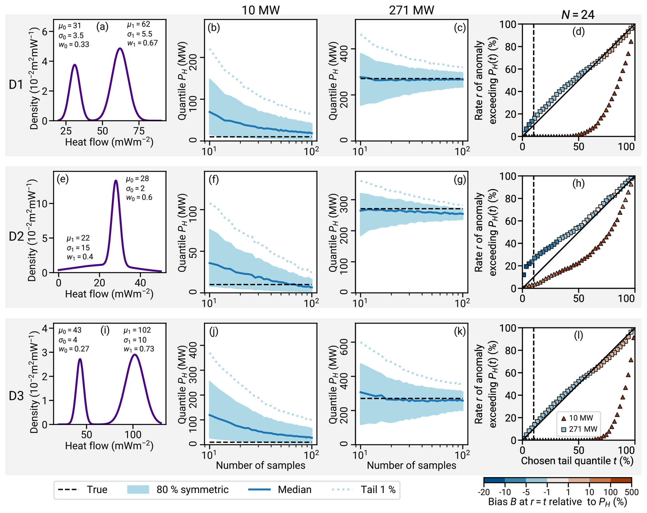
Figure 15 Resilience of the posterior distribution of Eq. (23) to violations of the gamma model hypothesis. We investigate how well REHEATFUNQ can quantify heat flow anomalies if the undisturbed regional aggregate heat flow follows a probability distribution that deviates from the gamma model. (a, e, i) Each graph shows the Gaussian mixture models D1 to D3 of that row (μ denotes mean, σ means standard deviation, and w means the weight of the mixture component). (b, f, j) Each graph shows quantiles of the posterior distribution given the synthetic regional PDF of the same row and a synthetic anomaly as in Fig. 13 with 10 MW of power over a fault length of 160 km (14 km depth). The anomaly profile follows Eq. (25). The quantiles are the median over a set of 1000 samples for each N. (c, g, k) The same for a 271 MW anomaly. (d, h, l) For N=24, the chosen tail quantile t is plotted against the rate r at which P_H(t) exceeds the true power P_H of the anomaly within the 1000 samples. The r=t correspondence is indicated as a solid line; the 10 % tail quantile is a dashed line. The marker fill color, corresponding to the color bar, indicates the difference in the t quantile (across the 1000 samples) of P_H(t) relative to the true power, that is, the bias at the actual exceedance rate t when using P_H(t). Negative values show that the anomaly is underestimated; positive values show that it is overestimated.

Figure 15 shows the median of the 1 %, 10 %, 50 %, and 90 % tail quantiles across 1000 samples from each distribution for a selection of sample sizes N between 10 and 100. With an increasing N, the posterior distribution becomes increasingly concentrated. In the case of the two bimodal distributions, the true anomaly strength P_H is captured within the 10 % and 90 % tail quantile for N>50. For a small N, the 10 % tail quantile is an upper limit on the anomaly strength, but the 90 % tail quantile (or equivalently 10 % quantile) is biased to larger values for P_H=10 MW. In the case of the unimodal distribution with longer tails, the true anomaly is larger than the range which 10 % to 90 % quantiles converge to at N=100; that is, the power of the anomaly is underestimated. In all cases, the median 1 % tail quantile is an upper bound across the investigated size of N≤100.

If the anomaly is strong (1.7 MW km⁻¹), its strength can generally be well quantified. The median typically follows the true anomaly strength closer than the width of the 80 % symmetric quantiles. Even in the exceptional case of distribution D2 for N→100, the 80 % symmetric quantile is close to the true frictional power.

If the anomaly is weak (62 kW km⁻¹), the posterior distribution overestimates P_H. Especially for $\text{10}\le N\le \text{20}$, the true anomaly P_H is located at or below the 90 % tail quantile. In the case of D3, the median overestimates P_H by a factor of 10 at N=10.

So far, the analysis has considered the median across the synthetic simulation (1000 samples) for each N. This ensemble view is useful to investigate the bias, but it does not fully reflect the inference problem on a particular fault. When considering the median of a tail quantile P_H(t) across the simulated set of samples, P_H(t) will be smaller than this median in 50 % of the cases. For instance, if the 10 % tail quantile P_H(10 %) straddles the strength of the anomaly at P_H=271 MW for distribution D2, its use would underestimate the anomaly with a 50 % chance if D2 were the true regional heat flow distribution.

This warrants investigating the relationship between a chosen tail quantile t and the resulting rate r of exceeding the corresponding power P_H(t). Figure 15d, h, and l show the relation between t and r for the three distributions of D1, D2, and D3 and for the two powers of 10 and 271 MW.

Depending on the actual power of the anomaly, two different behaviors can be observed. If the anomaly is low, the rate of exceeding the tail quantile is lower than chosen, r<t. Especially for D1 and D3, this effect is pronounced when t≲50 %, where r=0. This means that within the 1000 synthetic samples, none exceeded the tail quantile. A similar albeit less pronounced effect can be seen for D2. Hence, the small tail quantiles are hence a cautious estimate for a low P_H.

For a large P_H, the opposite occurs. At small tail quantiles, r>t and the size of the anomaly is underestimated. Depending on the distribution, the maximum excess of r at the 10 % tail quantile (t=10 %) is 4 % to 18 %. That is, there are 40 %–180 % more samples than desired in which the anomaly is underestimated.

The severity of this underestimation can be expressed by what we call the “bias” B. We define B to be the relative under- or overestimate of the true power P_H at the actual tail quantile t. Formally, if we express with ${\widehat{P}}_h(t,i)$ the power of the ith sample at the posterior tail quantile t and with ${\widehat{P}}_h\left(t\right)$ the tth (smallest) quantile of ${\widehat{P}}_h(t,i)$ among the generated samples, then we define B by

$$\begin{array}{}\text{(29)}& B={\displaystyle \frac{{\widehat{P}}_h\left(t\right)}{P_{\mathrm{H}}}}-\mathrm{1}.\end{array}$$

The purpose of B is to indicate the bias of ${\widehat{P}}_h$ as an estimator at the true rate of exceedance t. If B is negative, at a chance t the anomaly power P_H is underestimated by a fraction of B or more. If B is positive, the rate at which P_H exceeds ${\widehat{P}}_h$ is actually smaller than t and there is an overestimation of the power P_H by a factor of at least B among the 1−t largest ${\widehat{P}}_h(t,i)$ values (it would be 0 for the “unbiased” B=0).

For small frictional power, B is positive through nearly all of the range of t. At t≈10 %, for instance, we find B=40 %–610 % for P_H=10 MW. At a large P_H value, B is negative and ranges from −4 % to −9 %. Conclusively, there is a substantial margin for the quantification of small anomalies and a small underestimation for large anomalies.

The two effects also occur for a purely gamma-distributed heat flow sample, although they are less pronounced in underestimating a large P_H (in Fig. 16b, we find a maximum of 5 % underestimation at the 10 % tail quantile within the gamma distribution parameter space shown in Fig. 6).

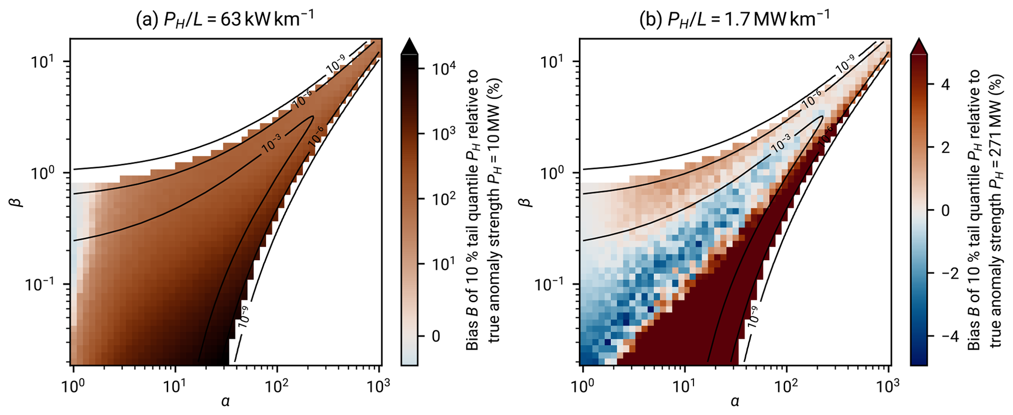
Figure 16 Bias B of the 10 % tail quantile for different gamma-distributed regional aggregate heat flow distributions. The bias (Eq. 29) quantifies how much the location ${\widehat{P}}_h\left(t\right)$ of the tail quantiles of the posterior distribution f(P_H), Eq. (23), interpreted as a frequentist exceedance interval, under- or overestimates the true anomaly power P_H at the ensemble's 10 % quantile of ${\widehat{P}}_h\left(t\right)$. A negative value indicates that the anomaly is underestimated by at least that amount in 10 % of 1000 generated samples. A positive value indicates that the anomaly is overestimated at the 10 % quantile of ${\widehat{P}}_h\left(t\right)$ and that the smallest estimate of P_H in that quantile is larger than P_H by the given amount of B. A value of B=0 indicates that the tail quantile coincides with the rate-t exceedance interval of the ensemble.

To conclude, the tests yield posterior support for our gamma model choice. The results derived from the three normal mixture distributions indicate that the frictional power generating a heat flow anomaly can be constrained even if the regional aggregate heat flow is not gamma distributed. Small tail quantiles (e.g., 1 % or 10 %) are typically larger than actual power P_H. If P_H is small, the small tail quantiles have a large margin to the actual power. This behavior occurs also for gamma-distributed aggregate heat flow so that it is likely an effect of the large ratio of heat flow standard deviation to anomaly amplitude. If the frictional power is small, the small tail quantiles might underestimate P_H, but the amount of this underestimation is relatively small.

Whether the posterior distribution can be used to quantify the heat flow anomaly further than giving an upper bound on its generating power depends on its amplitude and the sample size. If the frictional power is large compared to the fluctuation in the aggregate heat flow distribution – where in our setting an example of “large” is the 271 MW anomaly – the REHEATFUNQ model can quantify the heat flow anomaly throughout the sample size range of 10–100. The posterior distribution's median is meaningful, and the posterior distribution's 80 % centered quantile clearly separates from 0. If the frictional power is small compared to the fluctuations – here 10 MW – the posterior distribution's central quantiles lose their significance as best estimates and overestimate instead. This indicates that the bulk of the posterior distribution can be used as a confident estimate of the frictional power only if the heat flow anomaly is large compared to the heat flow variability or if the sample size is exceptionally large. Biases due to a differing distribution seem to have a relevant impact on this conclusion only at unrealistically large sample sizes (∼100 and beyond).

4.3 Physical limitations

Besides the statistical limitations discussed above, we discuss two physical limitations of the REHEATFUNQ model. One concerns both the regional aggregate heat flow distribution and the anomaly quantification, while the second is relevant only to the quantification of heat flow anomalies.

4.3.1 Regional aggregate heat flow distributions

The first limitation that affects both the inference of regional aggregate heat flow distributions and the quantification of heat flow anomalies is if the fluctuations are mostly due to random sampling of a spatially varying heat flow field (Fig. 2). The limitation is that the precision of the results cannot be arbitrarily increased by increasing the number of measurements (or at least this would not be obvious). As more and more measurements are taken, the full spatial variability will eventually be explored. In combination with the researchers' spatial measurement strategy, which will likely be systematic rather than random, all sources of “randomness” in the stochastic model of regional heat flow variability would eventually be exhausted. This limit is particularly important for the anomaly quantification, where at some point – read number of measurements – the ability to quantify an anomaly will be limited by the ability to disentangle a fixed spatial signal and not by a limited number of data.

The solution to these limitations is straightforward: first, given that the fluctuations were mainly due to a randomly sampled spatial field and a large number of heat flow measurements were available, this field should be clearly distinguishable in the point cloud of heat flow measurements (imagine adding 10 times more data points to Fig. 2). Hence the effect would not be a hidden effect. To account for the spatially varying field, geophysical modeling of the heat generation and transport can then help to detrend the data. This latter part can of course also help reduce the uncertainty if there are only few data points (see, e.g., Fulton et al., 2004).

4.3.2 Anomaly quantification

In Sect. 3.1, we have listed a number of possible origins of the regional fluctuation in surface heat flow. While the distinction between these origins is not relevant for the derivation of a regional aggregate heat flow distribution, it is important for the quantification of heat flow anomalies. In particular, it is important whether the heat flow fluctuations are due to inhomogeneous heat sources or transport that differs from homogeneous conduction. In nature, both effects can be relevant (e.g., Norden et al., 2020).

If the origin of the heat flow fluctuations is the heat source distribution, heat flow anomalies are truly independent from the stochastic process. This is the setting in which the analytical solutions to the heat flow problem based on simplified assumptions (e.g., Brune et al., 1969; Lachenbruch and Sass, 1980), including Eq. (25), can be applied.

If the origin of the heat flow fluctuations is, even partly, due to the heat transport, the separation of the heat flow anomaly from the regional fluctuations is not possible without taking this transport into account. Figure 17 illustrates this with the synthetic example of heat conduction from a buried strike-slip fault. The same spatially fluctuating heat flow field of panel c is generated by varying conduction in panel a and by varying thermal power density in panel b. While the undisturbed heat flow is the same in both configurations, the surface heat flow anomaly that is generated by the buried strike-slip fault differs considerably in panel d. While in the case of homogeneous conductivity the resulting anomaly resembles the analytical solution by Lachenbruch and Sass (1980, Eq. A22b), the anomaly is asymmetrically distorted by the inhomogeneous heat conduction. To infer the fault-generating power in the case of panel a, the heat conductivity field κ(x) needs to be known.

This is an application paradox: to separate a heat flow anomaly from fluctuations that are caused by the transport process, one would need detailed knowledge about this process – which in turn renders modeling the fluctuations by stochastic means unnecessary. The answer to this paradox is that the application of REHEATFUNQ requires that the heat transport equation is sufficiently known in the region of interest and thereafter allows for the separation of heat flow anomalies from the surface heat flow due to an unknown heat source distribution.

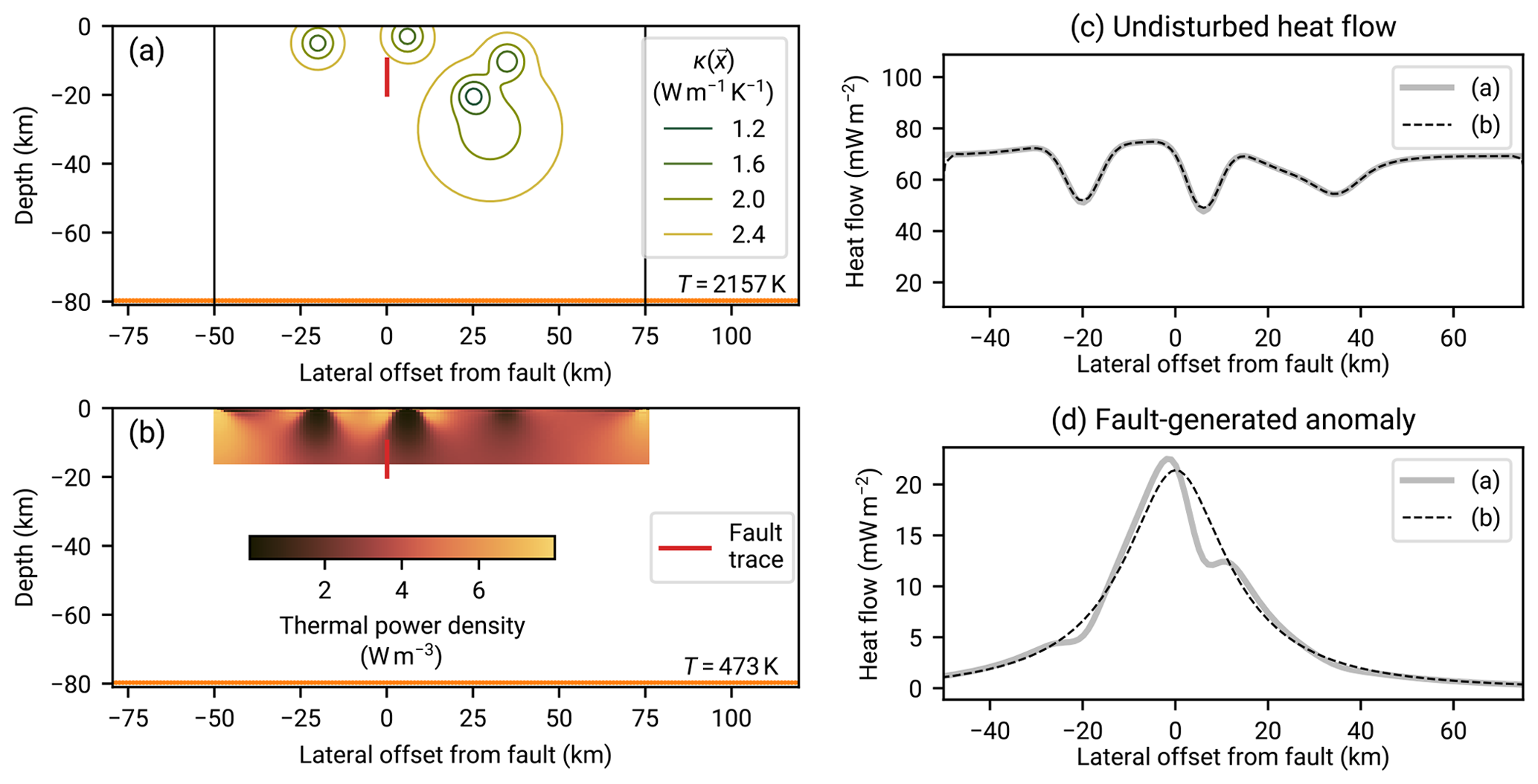
Figure 17 Two groups of heat flow fluctuation causes. Panels (a) and (b) illustrate heat flow fluctuations on the basis of inhomogeneous conductivity κ and by varying volumetric heat production. Both (a) and (b) are driven by a line heat source of constant temperature at 80 km depth (leading to an average upward heat flow of 68.3 and 40 mW m⁻² at κ=2.5 W m⁻¹ K⁻¹, respectively) and have a T=0 boundary condition at the surface. The additional heat sources in (b) are fit to match the surface heat flow in (a) (panel c shows the surface heat flow of both models). While both the varying conductivity and production can lead to similar fluctuations in surface heat flow, only the heterogeneous conductivity κ, panel (a), influences the anomaly, panel (d), generated by a buried strike slip fault (frictional power of 0.98 MW km⁻¹). If fluctuations are due to inhomogeneous sources, the heat flow anomaly is independent of the fluctuations. The thermal conductivity in panel (a) is varied within bounds similar to what Harlé et al. (2019) found for the Upper Rhine Graben (1–4 W m⁻¹ K⁻¹), and the heat production in panel (b) is varied within a range compatible with what Jaupart and Mareschal (2005) list for the Australian cratons (0–8 µW m⁻³).

5 Example: San Andreas fault

To demonstrate the REHEATFUNQ model, we apply it to the San Andreas fault (SAF) system in California. The SAF has a history of research regarding fault-generated heat flow in context of the discussion of whether the fault is frictionally weak or strong (Brune et al., 1969; Lachenbruch and Sass, 1980; Scholz, 2006). The argument brought forward by Brune et al. (1969) and refined by Lachenbruch and Sass (1980) starts with a comparison of the fault-lateral plot of a fault-generated surface heat flow anomaly with heat flow measurements close to the fault (up to ∼20–100 km distance). The lack of such an anomaly visible in the data is then used to derive an upper bound on the strength of the heat flow anomaly, that is, the frictional resistance at a given long-term fault slip rate. Visual inspection of the anomaly heat flow graphs are used to define a fuzzy upper bound on the frictional resistance above which the generated anomaly seems unlikely drawn against the data.

This discussion sparked the development of the REHEATFUNQ model; hence our work aims to contribute to the analysis. REHEATFUNQ aims to explore the fluctuation using a stochastic ansatz. The existence of a stochastic process might have a considerable impact on the analysis since the number of heat flow data in each of the regions investigated by Lachenbruch and Sass (1980) is rather small (6–19) and the fluctuations are on the order of the heat flow anomaly magnitudes. Furthermore, REHEATFUNQ aims to quantify the fuzziness of the assessment of which heat flow anomaly strengths are compatible with the data by means of the posterior distribution f(P_H) of Eq. (23).

Figure 18 Map of the regions investigated in Sect. 5. Heat flow data are from Lucazeau (2019), filtered as described in Sect. 2.1. The San Andreas fault trace is from Milner (2014).

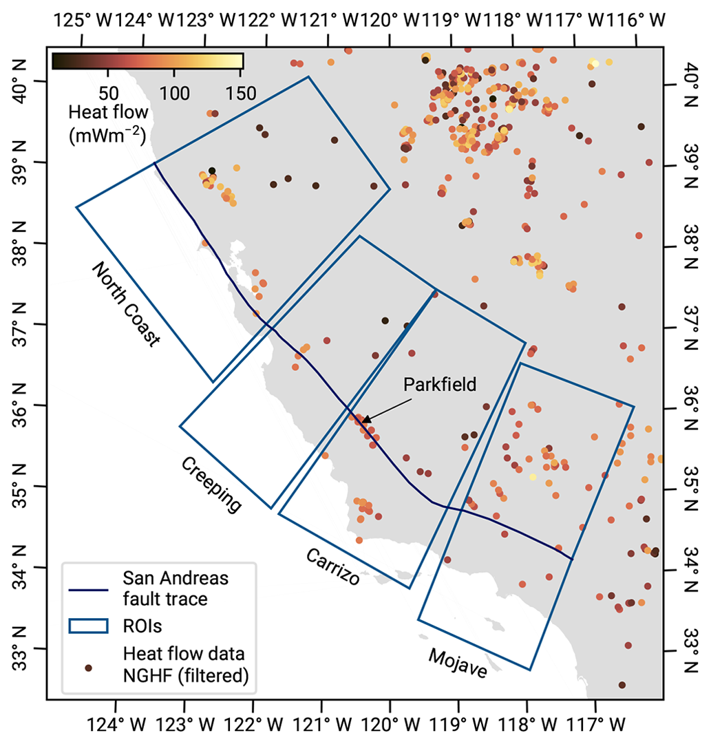
5.1 Regional aggregate heat flow

Figure 18 maps the regions investigated in this section, which we denote by Mojave, Carrizo, Creeping, and North Coast. The four regions can be understood as four distinct sections of the SAF. There are 49 (Mojave), 51 (Carrizo), 8 (Creeping), and 36 (North Coast) data points within the four sections. Figure 19 shows close-ups of the four regions. Therein, heat flow data clusters can be seen, and a number of data point pairs that violate the minimum-distance criterion can be identified. The range of heat flow varies across the four regions.

Figure 19 Closeups of the four regions of Fig. 18 and heat flow data within. The gray contour lines show the spatial heat flow field obtained by parameterizing the heat flow anomaly of Eq. (25) by the distance to the closest point on the fault trace.

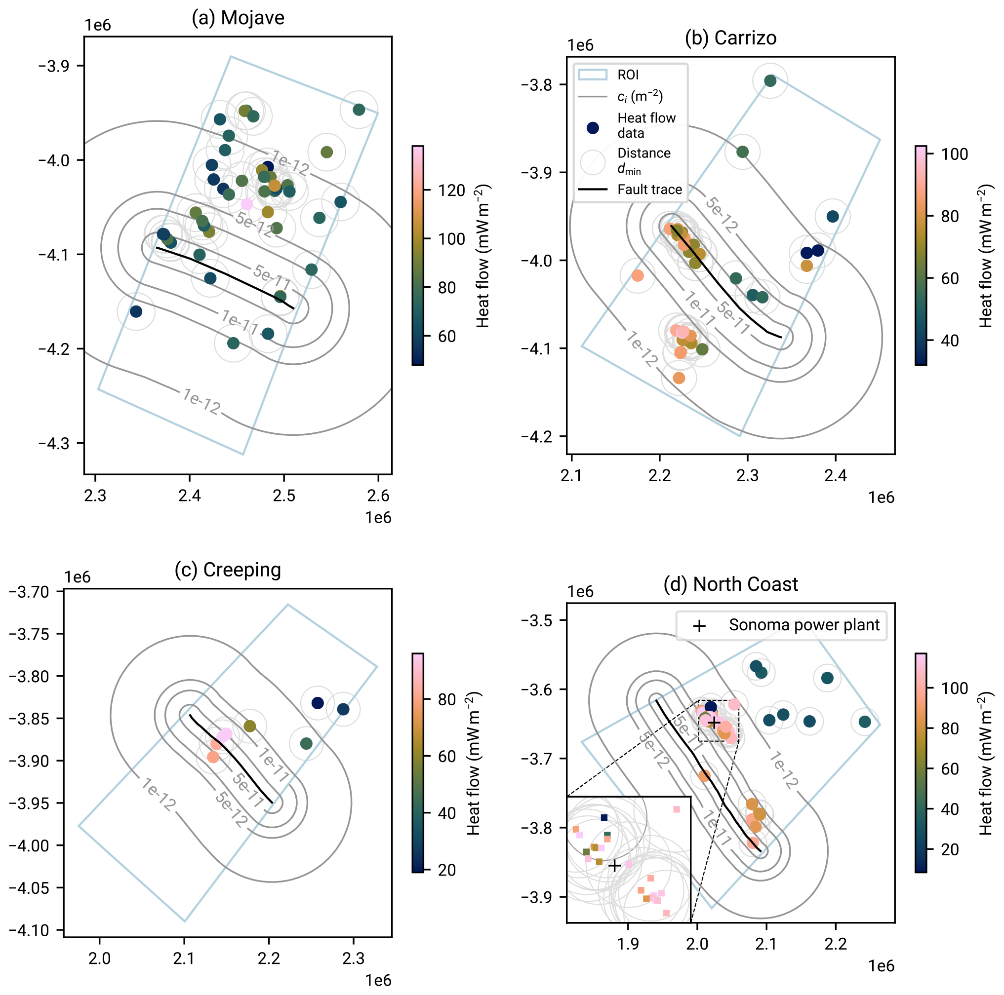
Figure 20 shows the posterior predictive distributions of regional aggregate heat flow for the four regions. The Mojave section in panels a and b is an example of a region that has a rather uniform data distribution and sufficient data to cover the regional aggregate distribution. The empirical CDF (eCDF) for all aggregate data within the region runs close to the center of the set of its random subsets that follow from enforcing the d_min=20 km minimum-distance criterion to prevent the pairwise clustering visible in Fig. 19a. Even though this reduces the density of points, the regional aggregate distribution is not significantly impacted by the thinning. This shows in the posterior predictive CDF in Fig. 20a and PDF in panel b. In both cases, the posterior predictive distribution closely follows the initial regional aggregate distribution.

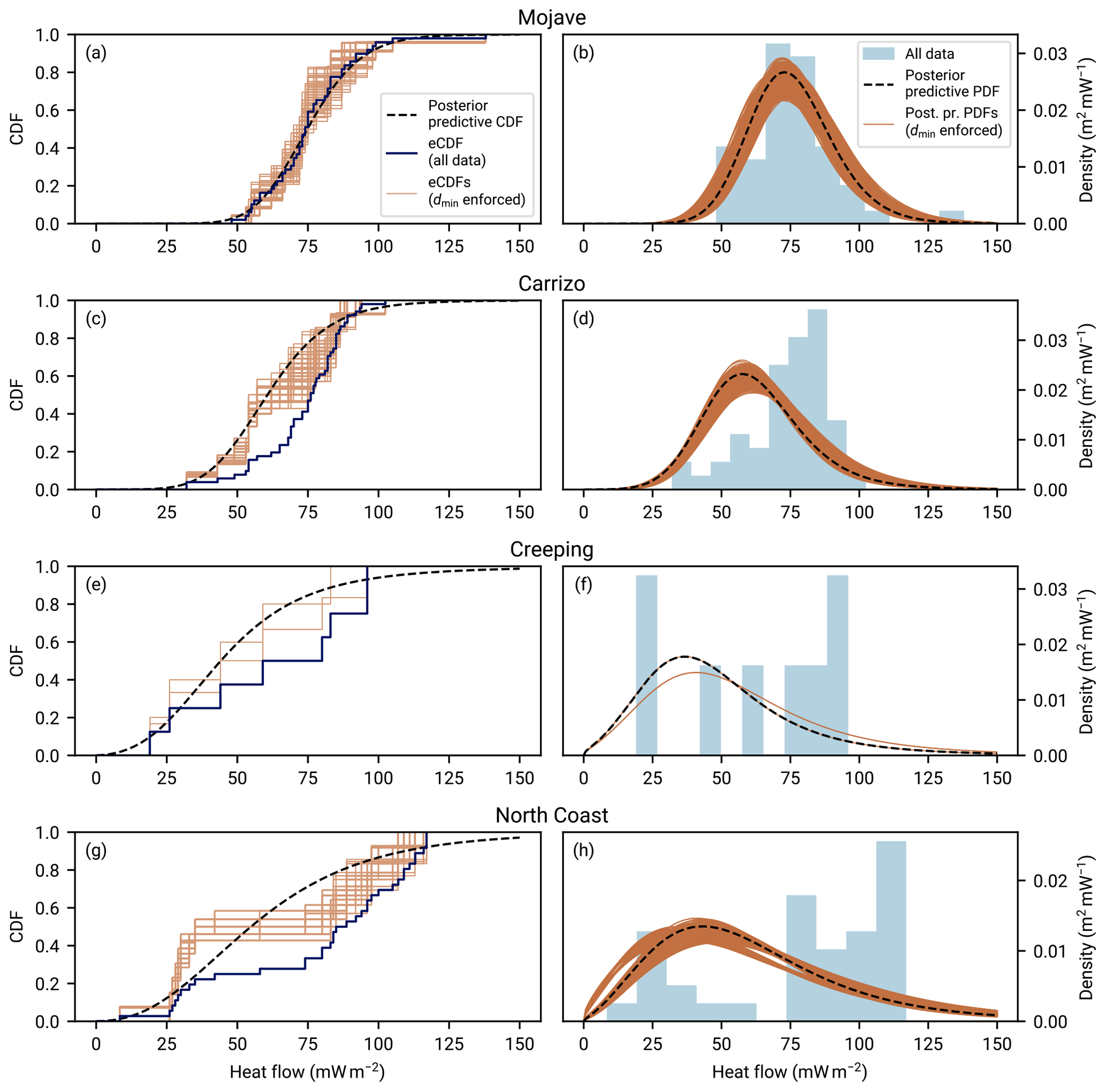
Figure 20 Posterior predictive distribution of regional aggregate heat flow for the four regions surrounding the SAF in Fig. 19. The left column, panels (a), (c), (e), and (g), shows the cumulative distribution of regional aggregate heat flow data from the NGHF within the region, denoted “eCDF (all data)”. The spatial distribution of these data is shown in Figs. 18 and 19. Since some data pairs are within 20 km of each other, the d_min sampling approach leads to the set of curves denoted “eCDFs (d_min enforced)”. The resulting posterior predictive CDF is shown as a dashed line. The right column, panels (b), (d), (f), and (h), shows the densities corresponding to the cumulative distributions of the left column. For each of the eCDFs with d_min enforced, the posterior predictive distribution of that data subset is shown. The results, in particular the differences between the histograms and the posterior predictive distribution estimates due to the distance criterion, are discussed in Sect. 5.1.

In the Carrizo section, the effect of spatial clustering and conversely of the exclusive treatment of the clusters' members stands out. The region contains a slightly larger number of data points (51), but the d_min-enforced eCDFs in panel c are more coarsely stepped than in the case of the Mojave section (panel a). The cause becomes evident in Fig. 19b, which shows that the data are concentrated mostly in two clusters, one covering the fault trace and one southwest of it. Only a few data points of each cluster are contained in each subset. Note that the two clusters are comprised mostly of high heat flow with respect to the remaining data points. As a result, the subsets' eCDFs and consequently the combined posterior predictive distribution are concentrated at lower heat flow compared to the initial regional aggregate distribution. Besides this thinning effect, the posterior predictive PDF in Fig. 20d seems to be the average of a number of subset predictive PDFs that cover a well-dispersed configuration space.

This is in contrast with the remaining two regions. The Creeping region, in panels e and f, contains only eight data points. Four of these data points, clustered across the fault trace, are pairwise within d_min. In particular, all four points are within 20 km of the data point closest to the fault. If this data point is contained in the subset, the remaining three largest heat flow measurements are excluded. Since the largest (pairwise exclusive) heat flow measurements are equal, this leads to only two distinct eCDFs in panel e and posterior predictive PDFs in panel f, both of which are controlled only by the selection of a single data point.

A similar effect occurs in the North Coast region, in panels g and h, with more data points (36). Many heat flow measurements are scattered around The Geysers geothermal field (see the location of the Sonoma power plant in Fig. 19). As a result, many of these points are pairwise exclusive under the d_min criterion. While most of the data in that cluster are at the upper end of the range within the region (>80 mW m⁻²), the lowest data point of the region (8.4 mW m⁻²) lies at the edge of the cluster (see Fig. 19d). This particular data point has significant control over the aggregate heat flow distribution: the two distinct shapes around which the set of subset posterior predictive distributions scatter in Fig. 20h correspond to the subsets in which the 8.4 mW m⁻² data point is included or not. Furthermore, two to three spatial clusters in Fig. 19d (The Geysers subset, the data close to the south end of the fault trace, and the data beyond the 10⁻¹² m⁻² contour) lead to distinct modes in the histogram in Fig. 20h.

5.2 Heat flow anomaly

Given the heat flow data from the previous section and the REHEATFUNQ gamma model, we can now investigate the strength of fault-generated heat flow anomalies originating from the SAF segments within the four regions. We assume a conductive mode of heat transfer and use the analytical model of Lachenbruch and Sass (1980) given in Eq. (25), parameterized by the distance to the closest point on the fault segment. We then use the parameterization of Eq. (26) to express the anomaly as a function of total frictional power P_H within the four regions. The depths of the fault segments are taken from the UCERF3 model (Milner, 2014). The resulting unit scaled factors c_i are shown in Fig. 19. This concludes step 4 of the workflow listed in Appendix A.

The resulting posterior distributions f(P_H) of the frictional power P_H are shown in Fig. 21 (step 5 of the workflow in Appendix A). They reflect features that we have discussed for the posterior predictive distributions ψ(P_H) in the previous section. As before, the Mojave section (panel a) features the clearest results. We have marked the frictional power of the “reference anomaly” of Lachenbruch and Sass (1980) (0.92 MW km⁻², leading to a total power of 146 MW over the fault segment), and we can confirm that this reference anomaly is unlikely. The REHEATFUNQ model yields less than 10 % posterior probability of anomalies of similar or larger frictional power. If one were to use the 10 % tail quantile as an upper bound on the fault's frictional power, the upper bound would be 111 MW corresponding to 0.77 “heat flow units” of Lachenbruch and Sass (1980). The best estimate of Lachenbruch and Sass (1980), 10 % of the reference anomaly corresponding to 14.6 MW, is within the bulk of the posterior mass. Under the premise of a stochastic interpretation of the heat flow data, the best estimate of Lachenbruch and Sass (1980) cannot reliably be distinguished from larger bounds within a factor of 8.

Figure 21 Posterior distributions of the frictional power P_H from the analysis of heat flow anomalies surrounding the fault segments in Fig. 19. The heat flow data and heat flow anomaly signature {c_i} used in the computation of the posterior distributions following Eq. (23) are also shown in Fig. 19. LS1980: Lachenbruch and Sass (1980).

In the Carrizo section (Fig. 21b), the existence or non-existence of a finite heat flow anomaly is less clear. The PDF has a finite mode between 50 and 100 MW that could indicate the existence of a heat flow anomaly, but the curve is not well-separated from 0. The origin of this peak becomes clear in Fig. 19b. On the one hand there is a high heat flow cluster just next to the north end of the fault segment compared to the northeastern part of the region, which could support the existence of an anomaly. On the other hand, the cluster south of the fault trace consists of similarly or exceedingly high heat flow, adding the ambiguity that the northern cluster could be due to the generally large range of heat flow from north to south. Hence, the existence of an anomaly is an option, but equally plausible is the overlay of an independent regional trend, for instance the Coast Ranges–Great Valley transition that Williams et al. (2004) modeled near Parkfield. More geophysical analysis would have to be performed to disentangle the posterior distribution for, say, P_H<175 MW (the 10 % tail quantile in Fig. 21b). Only the reference anomaly of Lachenbruch and Sass (1980) seems to be a large enough effect that it could be considered unlikely as is, being close to the 10 % tail quantile.

As before, the results for the Creeping and North Coast sections are of limited significance due to the data and geologic situation. In the Creeping section (Fig. 21c), there is one dominant mode at about 200 MW, but there is a long tail, with a few percent probability, up to about 1500 MW. The origin of this tail becomes clear when looking at the logarithm of the PDF (inset): the selection of data points from the cluster of four data points close to the fault trace leads to three separated peaks in the with modes at roughly 200, 500, and 1500 MW. While the mass associated with the two higher peaks is small, this example highlights that the identification of the frictional power P_H from very small data sets is aggravated by the dependency on individual data points. In this region, our data filtering has a profound effect (we retain 8 data points of the NGHF, while d'Alessio et al., 2006, for instance, use 49 data points) so that a detailed quality analysis of the data set is warranted for further refinement of the analysis.

In the North Coast section, the posterior distribution has a peak at roughly 300 MW. This is likely due to the generally higher heat flow close to the fault compared to the northeastern end of the region. The peak is broad, however, and a 90 % credibility interval surrounding the peak is not much smaller than 90 % of P_H domain (e.g., 325 MW from about 10 to 425 MW versus 450 MW). The reference anomaly is a bit below to the posterior distribution's median.

The fairly sharp separation into two regions parallel and north to the fault, one with high and one with low heat flow, has already been discussed by Lachenbruch and Sass (1980). They have proposed that the increased heat flow within 100 km of the fault trace might be due to a combination of an interaction with the subducting plate and frictional heating within the fault systems surrounding the SAF. This scenario is plausible within the data and highlights that the North Coast region is an example of a region where further geothermal modeling is required before REHEATFUNQ can separate the heat flow anomaly from the regional background heat flow.

In this section, we have used the expression given in Eq. (25) to model all heat flow anomalies. This allowed us to infer the uncertainty inherent to the anomaly quantification due to stochasticity in the heat flow data. What we have not captured in this simple analysis is the uncertainty in the heat flow anomaly itself. For instance in the case of the Creeping section, a localized creeping asperity and particular rock composition might cause an anisotropic heat flow anomaly (Brune, 2002; d'Alessio et al., 2006).

Figure 22 Anomaly quantification uncertainty reduction by decreasing heat flow data variance and increasing sample sizes. Panel (a) shows the synthetic regional aggregate heat flow distribution we start from. The gamma distribution has a mean of 75 mW m⁻² and standard deviation of 20 mW m⁻², which are similar to the posterior predictive distributions in the Mojave section (Fig. 20b). Panels (b) and (c) show the results of quantifying a fault-generated heat flow anomaly superposed on synthetic gamma-distributed regional aggregate heat flow distributions (the fault configuration is the same as that of Fig. 13 with a depth of d=14 km). In panel (b), the standard deviation of the distribution in (a) is reduced while keeping the mean and the sample size of N=20 constant. This could, for instance, be achieved by removing spatial trends through modeling. In panel (c), the standard deviation is kept constant while the sample size is increased. In both panels (b) and (c), the minimum-distance criterion is not enforced.

6 Conclusions

This study presented the REHEATFUNQ model for regional aggregate heat flow distributions and the quantification of heat flow anomalies. The REHEATFUNQ model is a new approach to the analysis of regional heat flow that aggregates the data into a single heat flow distribution that is agnostic to the spatial component of the data. Heat flow data are interpreted as the result of a stochastic process characteristic to the region. As a result, REHEATFUNQ treats the variability in heat flow measurements on short spatial scales by design and uses Bayesian inference both to estimate the regional aggregate heat flow distribution and to quantify the frictional power that generates a potential heat flow anomaly superposed on the regional heat flow. Thereby, REHEATFUNQ can quantify the uncertainty in estimating fault-generated heat flow anomalies from heat flow measurements.

REHEATFUNQ is an empirical model and uses the gamma distribution to model regional aggregate heat flow. Our goodness-of-fit analysis shows that the gamma distribution is not a perfect model. Yet, it is optimal in the sense that among other similarly simple probability distributions, none is clearly favorable to the gamma distribution. Furthermore, we have tested how resilient the heat flow anomaly quantification of REHEATFUNQ is to extreme deviations from the gamma distribution hypothesis inspired by real-world data. Our results show that REHEATFUNQ is successful in determining upper bounds on the strength of fault-generated heat flow anomalies under these conditions and that it can fairly well quantify the strength of an anomaly if the heat flow data set and the power of the anomaly are sufficiently large. We have found no indication that these results depend significantly on the region size up to a circumradius of 260 km.

In this article, we focused on the analysis of the heat flow anomaly generated by a vertical fault in a homogeneous half space (Lachenbruch and Sass, 1980), which is implemented in REHEATFUNQ. Other heat flow anomalies, obtained for instance from numerical methods, can easily be used by providing scale coefficients at the data locations. This might be especially important for complex fault geometries, in the case of inhomogeneous thermal conductivity or in the presence of convection.

An application of the REHEATFUNQ model to the San Andreas fault in California highlights that a stochastic interpretation of the heat flow data can significantly relax the upper bound for a fault-generated heat flow anomaly derived by Lachenbruch and Sass (1980). Their best estimate has an amplitude that is low enough such that random fluctuations might have hidden the anomaly. The stochastic approach underlying REHEATFUNQ is hence worth attention, and REHEATFUNQ can be a valuable tool for the analysis of regional heat flow values.

The reduction in regional heat flow variability through the correction of modeled geothermal patterns and a standardized heat flow data processing, including for instance the removal of topographic effects, may be the most promising path forward to reduce the uncertainties in the heat flow anomaly quantification. While Fig. 22 indicates that a reduction in heat flow variability leads to a proportional reduction in anomaly quantification uncertainty, the uncertainty reduction with an increased sample size scales sublinearly and requires orders of magnitude more (expensive) heat flow data than available today. Steps that can lead to such a reduction in heat flow variability are the unified correction for topographic effects as performed by Fulton et al. (2004) and detrending based on geothermal modeling (e.g., Cacace et al., 2013). An important aspect might also be the determination of boundaries between regions of (nearly) uniform heat flow characteristics. Our empirical analysis has shown that the mixture of two aggregate heat flow distributions, possibly resulting from the boundary between two such regions, is sufficient to explain the empirical mismatch of the gamma distribution model. Finally, the work of the International Heat Flow Commission to update the Global Heat Flow Database (Fuchs et al., 2021) might lead to a reduction in heat flow variability.

Appendix A: Workflow cheat sheet

Here we provide a short synopsis of a typical workflow that uses the REHEATFUNQ Python package (reheatfunq) to analyze regional aggregate heat flow and quantify the power of an underground heat source with a known surface heat flow pattern. Figure 8 accompanies this synopsis and illustrates important steps.

The workflow assumes that a region of interest (ROI) and a set of heat flow data available therein are given. Furthermore, the subject of the analysis is an underground heat source (the unknown heat source) whose surface heat flow pattern q_a(x) (the heat flow anomaly) can be computed but whose power P_H is unknown and should be inferred.

1. Filter the heat flow data. For instance, this might include the removal of any known unreliable measurements or known outliers.

2. Choose a minimum-distance parameter d_min. This parameter aims to reduce the impact of spatial data clusters by considering heat flow data as potentially dependent if they are located closer than d_min. In this article, we use d_min=20 km (see Sect. 3.2).

3. Remove any known spatial heat flow pattern from the heat flow data. This might include not only topographic effects (e.g., Fulton et al., 2004) but also the surface heat flow generated by a known underground heat source.

4. Compute the coefficients {c_i} that specify how much surface heat flow is generated at the heat flow data locations {x_i} by the unknown heat source per power P_H. This might be done by computing the surface heat flow anomaly q_a(x_i) at the locations of the heat flow measurements {q_i} for an arbitrary power P_H and dividing the result by that power ($c_i=q_{\mathrm{a}}\left({\mathit{x}}_i\right)/P_{\mathrm{H}}$). Any external method can be used to solve the conduction–advection equation for the problem at hand (heat source distribution and boundary conditions) as long as q_a(x) can be evaluated at the heat flow data locations and P_H is known. The AnomalyNearestNeighbor class can be used to provide the coefficients c_i to the REHEATFUNQ model. The REHEATFUNQ package provides furthermore the solution (A23b) of Lachenbruch and Sass (1980) for an infinitely long, surface-rupturing straight strike-slip fault in a homogeneous half space (AnomalyLS1980). Figure 8a shows how this anomaly may look compared to some artificial heat flow data.

5. Evaluate the posterior distribution of the unknown heat source's power P_H. Use the HeatFlowAnomalyPosterior class to compute the posterior PDF, CDF, complementary CDF (“tail distribution”), and tail quantiles of the power P_H. Figure 8c shows what the posterior PDF looks like for the example in Fig. 8a: the heat flow anomaly was successfully assessed, but due to the scatter in the data, the result is uncertain.

Code examples can be found in the documentation shipped with the REHEATFUNQ source code (Ziebarth, 2023) and online at https://mjziebarth.github.io/REHEATFUNQ/ (last access: 25 March 2024). All analysis performed in this article can be reproduced using the Jupyter Notebooks (Kluyver et al., 2016) provided with the source code.

Appendix B: Random global R-disk coverings

In the analyses, we frequently make use of random global R-disk coverings (RGRDCs). The RGRDC is an algorithm to generate a set of many regional aggregate heat flow distributions from the NGHF data set by means of random sampling. The algorithm allows us to capture the typical variability in heat flow within the global database. Control over the radius R allows us to investigate the global data set over various spatial scales.

In the RGRDCs, disks are randomly distributed across Earth's surface to asymptotically capture the detail of the inhomogeneous data set. Within each disk, data from the filtered NGHF are selected and form one regional aggregate heat flow distribution. In detail, the algorithm proceeds as follows.

• 1.

  Filter the NGHF according to general criteria. All remaining points are unmarked.

• 2.

  Draw 100 000 random points {p_i} from a spherical uniform distribution.

• 3.

  Perform the following for each of them.

  • (a)

    Collect the set {x_i} of NGHF data points within a distance R of p_i. If any of them are marked, discard p_i and continue with p_i+1.

  • (b)

    Ensure a minimum distance d_min between the {x_i} to prevent biases from spatial measurement clusters (see Sect. 3.2). From violating data point pairs, keep one data point at random until the criterion is fulfilled for all remaining {x_i} values.

  • (c)

    If the number of remaining {x_i} is larger than 10, retain the disk centered on p_i. The remaining {x_i} are the corresponding regional heat flow sample and are marked.

• 4.

  Repeat from step 1 M times to obtain M coverings.

Figure 1a shows the location of the R disks (R=80 km) that have been determined for later use in Sect. 3.3.2.

B1 Synthetic random global R-disk coverings

To understand how well our gamma distribution model of regional heat flow can describe the data from the RGRDCs obtained from the NGHF database, we generate synthetic coverings from the gamma distribution model and compare statistics of the NGHF coverings with those of the synthetic coverings. To be able to do so, the synthetic coverings need to replicate the sample size structure and the heat flow distribution of the NGHF data coverings. Furthermore, the same data filtering needs to be applied. To this end, we use the following algorithm to generate M synthetic RGRDCs.

• 1.

  Generate a set $\mathcal{X}=\mathit{\{}{X}_{\mathrm{1}},\mathrm{\dots },X_n\mathit{\}}$ of random global R-disk coverings $X_i=\mathit{\{}{Q}_{\mathrm{1}}^i,\mathrm{\dots },Q_{m\left(i\right)}^i\mathit{\}}$ from the NGHF database (see Appendix B).

• 2.

  For each heat flow distribution $Q_j^i=\mathit{\{}{q}_{\mathrm{1}},\mathrm{\dots },q_{l(i,j)}\mathit{\}}$, compute the gamma distribution maximum likelihood parameters (k_ij,θ_ij).

• 3.

  Repeat the following M times.

  • (a)

    Select a random NGHF covering X_i.

  • (b)

    For each heat flow distribution $Q_j^i$ within X_i, proceed as follows.

    • i.

      Generate a heat flow sample of at least l(i,j) data points. Draw these heat flow values from a gamma distributions with parameters (k_ij,θ_ij).

    • ii.

      For each heat flow value from the sample, draw a random standard deviation σ from the relative error distribution (Fig. 9). From a central normal distribution with that σ, draw a random relative error. Distort the corresponding heat flow value by this relative error.

    • iii.

      Round all heat flow values from the sample to integers.

    • iv.

      Remove all negative heat flow values and all those larger than 250 mW m⁻².

    • v.

      If less than l(i,j) data points remain, repeat. Otherwise the first l(i,j) accepted heat flow values will form the jth heat flow distribution within the current synthetic covering.

  • (c)

    The generated synthetic covering will match the sample sizes of X_i and have, within the bounds imposed by the gamma distribution and the additional effects, a similar heat flow distribution.

Appendix C: Points-of-interest measurement model

This section considers a toy model that aims to mimic a data acquisition process in which few explorative measurements are joined by many dependent measurements that focus on the vicinity of particularly interesting previous measurements. We call these previous measurements “points of interest” (POIs). One might imagine that they represent a geothermal or oil field in which, after its discovery, many data points scatter in close proximity.

The POI model consists of an algorithm that distributes a desired number of sampling points {x_k} on a rectangular spatial domain. Synthetic heat flow measurements are generated for these points by querying a pre-generated spatial heat flow field q(x) on the spatial domain. This heat flow field q(x) is represented by a raster filled with values q_ij which are in turn drawn from a gamma distribution. Hence, if the points x_k were uniformly distributed, the resulting heat flow sample would follow a gamma distribution (up to discretization effects of the finite raster). With the POI spatial sampling, this is not the case.

Figure C1 The point-of-interest (POI) sampling algorithm to generate heat flow data sets with spatial clustering described in Appendix C. (a) The algorithm generated 100 random sampling points. Each point had a 20 % chance of becoming a POI (squares) and being randomly distributed over the square. At 70 % probability, a new point would be dependent and generated within an 8 km square surrounding a previous POI (triangles). At 10 %, the point would be randomly distributed but not of interest (circles). The coloring of the markers and the dashed circles surrounding some points illustrates the d_min sampling: only the filled black markers are used for the analysis in this particular sample, ignoring all data points within the d_min disks surrounding them. Panels (b) and (c) show the impact that the POI point generation and the d_min sampling have on the aggregate heat flow distribution. Panel (b) shows the empirical cumulative distribution function (eCDF) of the full data set as well as the CDF of the corresponding gamma distribution maximum likelihood estimate (MLE). Panel (c) shows the same for only the selected data points of panel (a). Deviations of the eCDF from the CDF in panel (a) due to the clustered sample points (steep slopes in the eCDF) are successfully removed in panel (c).

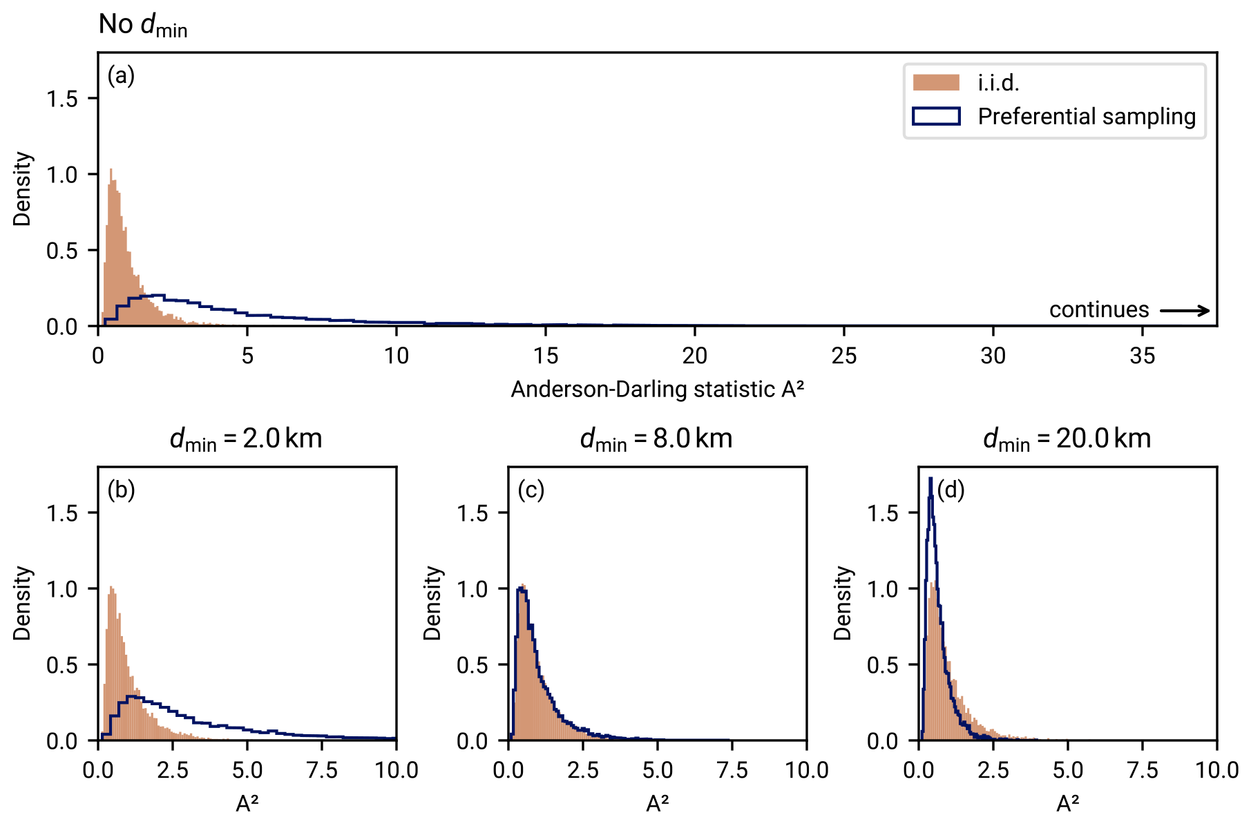
Figure C2 Improvement of the gamma distribution likeness of heat flow samples generated by the point-of-interest (POI) sampling method (Appendix C) when using the minimum-distance sampling. Each panel shows the distribution of the Anderson–Darling statistic A² (Stephens, 1986) for the gamma distribution, a measure of how well the sample matches the gamma distribution (less being a better match). The filled histograms labeled “i.i.d.” show the distribution of A² that follows from independent and identically distributed gamma random variables with α=10. The histograms marked by the dark-blue line show the distribution of A² generated from the POI sampling method with a gamma landscape generated for α=10 (shown in Fig. C1) and with P_POI=20 %, P_f=70 %, and R=8 km. The minimum-distance criterion has then been applied with the d_min specified in the panel titles. The good match between both distributions in panel (c) shows that an accurately chosen d_min can counter the spatial clustering effect of the POI sampling model. If d_min is chosen to be too small, the clustering is not effectively countered and a large A² compared to the i.i.d. histograms indicates significant departures from the gamma distribution. If d_min is chosen to be too large, the heat flow data generated from the POI model show less difference to the gamma distribution CDF than the actual i.i.d. gamma random variable. This is due to the minimum-distance criterion removing too many clusters, that is, also those clusters that naturally appear for uniform random variables.

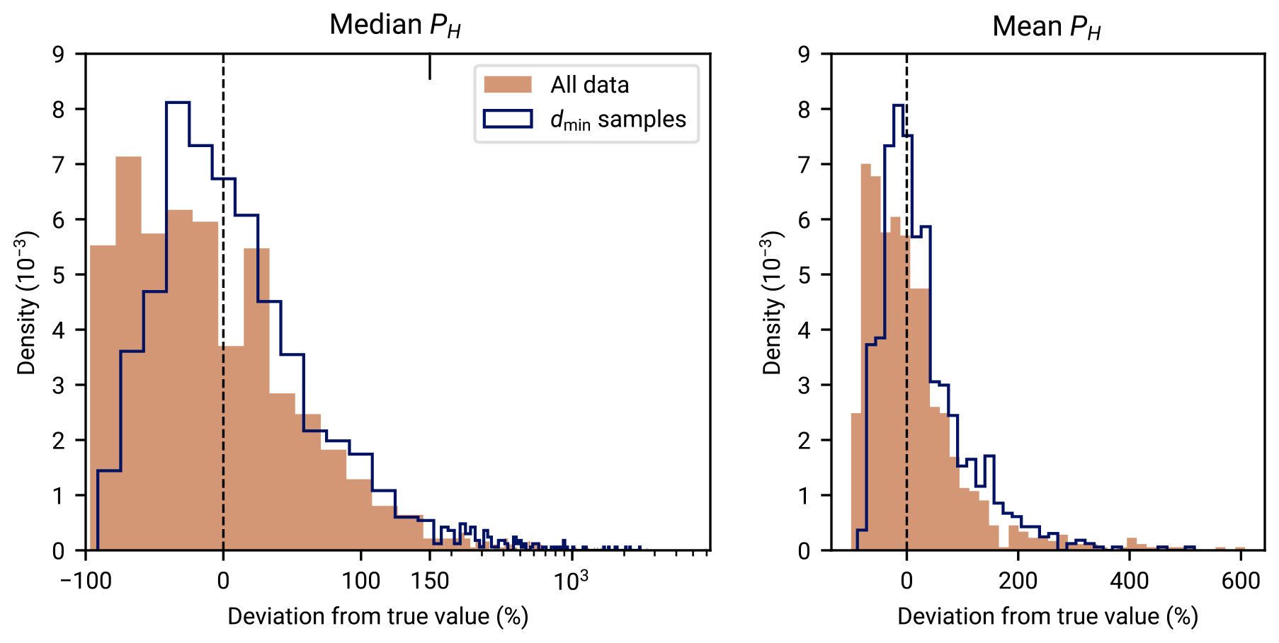
Figure C3 Improvement of the accuracy of the posterior P_H estimates for point-of-interest-generated (POI-generated) data as the minimum-distance sampling is enforced. Both panels analyze data generated from 1000 POI sampling runs with P_POI=12 %, P_f=80 %, R=5 km, and the gamma-distributed field in Fig. C1. The sample size is N=50, and d_min is 5 km. Panel (a) shows how the relative deviation of the P_H posterior distribution's median from the true P_H is distributed across the 1000 POI runs. For each run, the P_H posterior distribution is evaluated on all data (d_min=0) and with the minimum distance enforced (d_min=5 km). Using the minimum-distance criterion improves the accuracy of the median estimator. Panel (b) shows the same for the posterior mean P_H. Similarly, the use of the minimum-distance criterion reduces bias.

The POI sampling algorithm, illustrated in Fig. C1a, proceeds as follows.

• 1.

  Generate a rasterized heat flow field q(x) by drawing i.i.d. random values from a gamma distribution for each point of the raster.

• 2.

  Iteratively flip random pixel pairs of the heat flow raster q_ij if the flip reduces the variance in the local neighborhoods of the both pixels. This smoothens the field while retaining its aggregate gamma distribution.

• 3.

  Generate a first POI from a uniform distribution across the spatial domain.

• 4.

  Sequentially for each of the remaining N−1 requested points, choose one of the following actions.

  • (a)

    With probability P_POI, generate a new POI.

  • (b)

    With probability P_f, generate a follow-up point. Choose one of the existing POIs at random and place the follow-up point within a square of side length R of the selected POI.

  • (c)

    With remaining probability, generate a non-POI point uniformly in the spatial domain.

• 5.

  For each of the generated points, determine the measured heat flow value from the heat flow field q(x).

The general idea of this clustered point sampling is reflected in the assumptions made in the formulation of the REHEATFUNQ likelihood in Sect. 3.3.1. In the POI sampling, the dependent sampling points that attach to a POI lead to correlations in the aggregate heat flow distribution (see Fig. C1b) due to the spatial correlation of the underlying heat flow field. One point of the cluster – the POI – is spatially independent and leads to a random gamma-distributed heat flow measurement. Assumption II of Sect. 3.3.1 takes this into account by using only one data point of a cluster identified by the d_min disk at the same time. Assumption III then acknowledges that each point of the cluster is equally likely to be the independent, and the summation over all possible choices for independent points (latent parameter j) ensures that no data point is left behind.

In Fig. C1c, we can indeed observe that the enforcement of d_min results in more gamma-like samples compared to the full data set (panel b). We have furthermore observed from Monte Carlo simulations of the POI sampling that the likelihood approach in Eq. (5) leads to more accurate recovery of the true regional aggregate heat flow distribution (Fig. C2) and reduces bias in the estimation of heat flow anomalies (Fig. C3) when compared to using all heat flow data in the presence of spatial clustering.

Appendix D: Expressions for numerical quadrature

D1 Gamma conjugate prior distribution

The normalization constant Φ of Eq. (9) requires one numerical quadrature for the evaluation of the α integral. To this end, we first compute the location of the integrand's maximum α_max using an approximation based on Stirling's formula,

$$\begin{array}{}\text{(D1)}& {\displaystyle }{\mathit{\alpha }}_{\mathrm{0}}=\exp \left({\displaystyle \frac{\ln p-\mathit{\nu }s+\mathit{\nu }\ln \mathit{\nu }}{n-\mathit{\nu }}}\right),\end{array}$$

followed by a Newton–Raphson refinement. Integration is then performed in the intervals [α_min, α_max] and [α_max, ∞[ using tanh-sinh and exp-sinh quadrature, respectively (Takahasi and Mori, 1974; Tanaka et al., 2009). To prevent the integrand from overflowing, we use a transform of the type

$$\begin{array}{}\text{(D2)}& {\displaystyle }f\left(\mathit{\alpha }\right)\to \exp \left(\ln f\right(\mathit{\alpha })-\ln f({\mathit{\alpha }}_{\text{max}}\left)\right),\end{array}$$

where f is the integrand of Eq. (9) and ln f is expressed through the logarithmic versions of its constituents. This rescaling cancels in normalization.

The piecewise integrals involved in evaluating the posterior predictive CDF at a set of points {q_i} for a given Φ are computed using adaptive Gauss–Kronrod quadrature (Laurie, 1997; Kronrod, 1965; Gonnet, 2012).

D1.1 Kullback–Leibler divergence

The Kullback–Leibler divergence K is given in Eq. (14). For the gamma conjugate prior distribution with variables $\mathit{x}=(\mathit{\alpha },\mathit{\beta })$, the expression reads

$$\begin{array}{}\text{(D3)}& \begin{array}{rl}& K\left(\mathit{\varphi }\right(\mathit{\alpha },\mathit{\beta }),{\mathit{\varphi }}_{\mathrm{ref}}(\mathit{\alpha },\mathit{\beta }\left)\right)\\ & =\underset{{\mathit{\alpha }}_{\min }}{\overset{\mathrm{\infty }}{\int }}\mathrm{d}\mathit{\alpha }\underset{\mathrm{0}}{\overset{\mathrm{\infty }}{\int }}\mathrm{d}\mathit{\beta }{\displaystyle \frac{\mathrm{1}}{\mathrm{\Phi }}}{\displaystyle \frac{{\mathit{\beta }}^{\mathit{\nu }\mathit{\alpha }-\mathrm{1}}{p}^{\mathit{\alpha }-\mathrm{1}}{e}^{-s\mathit{\beta }}}{\mathrm{\Gamma }(\mathit{\alpha }{)}^n}}\\ & \cdot \ln \left({\displaystyle \frac{{\mathrm{\Phi }}_{\mathrm{ref}}}{\mathrm{\Phi }}}{\displaystyle \frac{{\mathit{\beta }}^{\mathit{\nu }\mathit{\alpha }-\mathrm{1}}{p}^{\mathit{\alpha }-\mathrm{1}}{e}^{-s\mathit{\beta }}\mathrm{\Gamma }(\mathit{\alpha }{)}^{n_{\mathrm{ref}}}}{{\mathit{\beta }}^{{\mathit{\nu }}_{\mathrm{ref}}\mathit{\alpha }-\mathrm{1}}{p}_{\mathrm{ref}}^{\mathit{\alpha }-\mathrm{1}}{e}^{-s_{\mathrm{ref}}\mathit{\beta }}\mathrm{\Gamma }(\mathit{\alpha }{)}^n}}\right),\end{array}\end{array}$$

where $(p,s,n,\mathit{\nu })$ are the parameters of ϕ with normalization Φ, $(p_{\mathrm{ref}},s_{\mathrm{ref}},n_{\mathrm{ref}},{\mathit{\nu }}_{\mathrm{ref}})$ belong to the reference model ϕ_ref with normalization Φ_ref, and Γ(α) is the gamma function. After a bit of algebra, the integrals can be converted to the following expression (with K being shortened notation in the following):

$$\begin{array}{}\text{(D4)}& \begin{array}{rl}K& =\ln \left({\displaystyle \frac{{\mathrm{\Phi }}_{\mathrm{ref}}}{\mathrm{\Phi }}}\right)+{\displaystyle \frac{\mathrm{1}}{\mathrm{\Phi }}}\underset{{\mathit{\alpha }}_{\min }}{\overset{\mathrm{\infty }}{\int }}\mathrm{d}\mathit{\alpha }{\displaystyle \frac{p^{\mathit{\alpha }-\mathrm{1}}}{\mathrm{\Gamma }(\mathit{\alpha }{)}^n}}\\ & \cdot [\left((\mathit{\alpha }-\mathrm{1})\ln {\displaystyle \frac{p}{p_{\mathrm{ref}}}}-\mathrm{\Delta }n\ln \mathrm{\Gamma }\left(\mathit{\alpha }\right)\right)\underset{\mathrm{0}}{\overset{\mathrm{\infty }}{\int }}\mathrm{d}\mathit{\beta }{\mathit{\beta }}^{\mathit{\nu }\mathit{\alpha }-\mathrm{1}}{e}^{-s\mathit{\beta }}\\ & -\mathrm{\Delta }s\underset{\mathrm{0}}{\overset{\mathrm{\infty }}{\int }}\mathrm{d}\mathit{\beta }{\mathit{\beta }}^{\mathit{\nu }\mathit{\alpha }}{e}^{-s\mathit{\beta }}\\ & +\mathit{\alpha }\mathrm{\Delta }\mathit{\nu }\underset{\mathrm{0}}{\overset{\mathrm{\infty }}{\int }}\mathrm{d}\mathit{\beta }\ln \left(\mathit{\beta }\right){\mathit{\beta }}^{\mathit{\nu }\mathit{\alpha }-\mathrm{1}}{e}^{-s\mathit{\beta }}],\end{array}\end{array}$$

where we have used the abbreviations

$$\begin{array}{}\text{(D5)}& {\displaystyle }\mathrm{\Delta }s=s-s_{\mathrm{ref}},\mathrm{\Delta }n=n-n_{\mathrm{ref}},\text{ and }\mathrm{\Delta }\mathit{\nu }=\mathit{\nu }-{\mathit{\nu }}_{\mathrm{ref}}.\end{array}$$

The three β integrals can be evaluated analytically with a little help from SymPy (Meurer et al., 2017):

$$\begin{array}{}\text{(D6)}& {\displaystyle }\underset{\mathrm{0}}{\overset{\mathrm{\infty }}{\int }}\mathrm{d}\mathit{\beta }{\mathit{\beta }}^{\mathit{\nu }\mathit{\alpha }-\mathrm{1}}{e}^{-s\mathit{\beta }}={\displaystyle \frac{\mathrm{\Gamma }\left(\mathit{\nu }\mathit{\alpha }\right)}{s^{\mathit{\alpha }\mathit{\nu }}}},\text{(D7)}& {\displaystyle }\underset{\mathrm{0}}{\overset{\mathrm{\infty }}{\int }}\mathrm{d}\mathit{\beta }{\mathit{\beta }}^{\mathit{\nu }\mathit{\alpha }}{e}^{-s\mathit{\beta }}={\displaystyle \frac{\mathrm{\Gamma }(\mathit{\nu }\mathit{\alpha }+\mathrm{1})}{s^{\mathit{\alpha }\mathit{\nu }+\mathrm{1}}}},\text{(D8)}& {\displaystyle }\underset{\mathrm{0}}{\overset{\mathrm{\infty }}{\int }}\mathrm{d}\mathit{\beta }\ln \left(\mathit{\beta }\right){\mathit{\beta }}^{\mathit{\nu }\mathit{\alpha }-\mathrm{1}}{e}^{-s\mathit{\beta }}={\displaystyle \frac{\left(\mathit{\psi }\right(\mathit{\alpha }\mathit{\nu })-\ln s)\mathrm{\Gamma }(\mathit{\nu }\mathit{\alpha }+\mathrm{1})}{\mathit{\alpha }\mathit{\nu }{s}^{\mathit{\nu }\mathit{\alpha }}}},\end{array}$$

where ψ(x) is the digamma function. After some more algebra, the expression used in REHEATFUNQ to estimate the Kullback–Leibler divergence from the reference model $(p_{\mathrm{ref}},s_{\mathrm{ref}},n_{\mathrm{ref}},{\mathit{\nu }}_{\mathrm{ref}})$ to the model $(p,s,n,\mathit{\nu })$ is

$$\begin{array}{}\text{(D9)}& \begin{array}{rl}K& =\ln \left({\displaystyle \frac{{\mathrm{\Phi }}_{\mathrm{ref}}}{\mathrm{\Phi }}}\right)+{\displaystyle \frac{\mathrm{1}}{\mathrm{\Phi }}}\underset{{\mathit{\alpha }}_{\min }}{\overset{\mathrm{\infty }}{\int }}\mathrm{d}\mathit{\alpha }{\displaystyle \frac{p^{\mathit{\alpha }-\mathrm{1}}\mathrm{\Gamma }\left(\mathit{\nu }\mathit{\alpha }\right)}{s^{\mathit{\nu }\mathit{\alpha }}\mathrm{\Gamma }(\mathit{\alpha }{)}^n}}\\ & \cdot \left[\right(\mathit{\alpha }-\mathrm{1})\ln {\displaystyle \frac{p}{p_{\mathrm{ref}}}}-\mathrm{\Delta }n\ln \mathrm{\Gamma }(\mathit{\alpha })-{\displaystyle \frac{\mathit{\nu }\mathit{\alpha }\mathrm{\Delta }s}{s}}\\ & +\mathit{\alpha }\mathrm{\Delta }\mathit{\nu }\left(\mathit{\psi }\right(\mathit{\nu }\mathit{\alpha })-\ln s)].\end{array}\end{array}$$

The integral (D9) is solved in REHEATFUNQ using the tanh-sinh integration routine implemented in the Boost C++ library (Takahasi and Mori, 1973). The bracketed part of the integrand in Eq. (D9) typically has a change in sign, which we have observed to lead to a condition number ($L_{\mathrm{1}}/\left|Q\right|$, where L₁ is the integral of the absolute integrand and Q is the integral of the signed integrand) of ∼10³. This is indicative of a precision loss of three digits (Agrawal et al., 2022), but we have not observed further numerical difficulties that could lead to great loss of usefulness.

D2 P_H marginal posterior distribution normalization

Evaluating the integrand of the marginal posterior distribution of Eq. (23),

$$\begin{array}{}\text{(D10)}& \begin{array}{rl}& \mathit{\gamma }\left(\mathit{\right\{}{\mathrm{\Delta }}_i{\mathit{\}}}_j;\mathit{\alpha },\mathit{\beta }\left)\mathit{\varphi }\right(\mathit{\alpha },\mathit{\beta })\\ & \sim {\displaystyle \frac{{\mathit{\beta }}^{{\mathit{\nu }}^{\prime }\mathit{\alpha }-\mathrm{1}}{\left(p\prod _{i\in {\mathcal{I}}_j}{\mathrm{\Delta }}_i\right)}^{\mathit{\alpha }-\mathrm{1}}\exp \left(-\left(s+\sum _{i\in {\mathcal{I}}_j}{\mathrm{\Delta }}_i\right)\mathit{\beta }\right)}{\mathrm{\Gamma }(\mathit{\alpha }{)}^{n+N_j}}},\\ & {\mathit{\nu }}^{\prime }=\mathit{\nu }+N_j,{\mathrm{\Delta }}_i=q_i-P_{\mathrm{H}}{c}_i\end{array}\end{array}$$

where N_j is the number of data points indexed in ℐ_j, leads to the modified hyperparameter update rule

$$\begin{array}{}\text{(D11)}& \begin{array}{rl}& \mathit{\nu }\to {\mathit{\nu }}_j^{\prime }=\mathit{\nu }+N_j,n\to n_j^{\prime }=n+N_j,\\ & s\to s_j^{\prime }=s+\sum _{i\in {\mathcal{I}}_j}(q_i-P_{\mathrm{H}}{c}_i),\\ & p\to p_j^{\prime }=p\prod _{i\in {\mathcal{I}}_j}(q_i-P_{\mathrm{H}}{c}_i),\end{array}\end{array}$$

given a sample {q_i}_j of N_j regional heat flow measurements. Since P_H occurs both in s and p and nonlinearly in the latter, it breaks the conjugacy of the prior distribution; i.e. the posterior distribution does not have the same functional shape. Additionally the normalization constant changes:

$$\begin{array}{ll}{\displaystyle }\mathcal{F}& {\displaystyle }=\sum _{j=\mathrm{1}}^m\underset{\mathrm{0}}{\overset{P_{\mathrm{H}}^{\mathrm{m}}}{\int }}\mathrm{d}{P}_{\mathrm{H}}\underset{\mathrm{0}}{\overset{\mathrm{\infty }}{\int }}\mathrm{d}\mathit{\beta }\underset{\mathrm{0}}{\overset{\mathrm{\infty }}{\int }}\mathrm{d}\mathit{\alpha }{\displaystyle \frac{{\mathit{\beta }}^{{}^{{\mathit{\nu }}_j^{\prime }\mathit{\alpha }-\mathrm{1}}}(p_j^{\prime }{)}^{{}^{\mathit{\alpha }-\mathrm{1}}}\exp \left(-s_j^{\prime }\mathit{\beta }\right)}{\mathrm{\Gamma }(\mathit{\alpha }{)}^{{}^{n_j^{\prime }}}}}\\ {\displaystyle }& {\displaystyle }=\sum _{j=\mathrm{1}}^m\underset{\mathrm{0}}{\overset{P_{\mathrm{H}}^{\mathrm{m}}}{\int }}\mathrm{d}{P}_{\mathrm{H}}\underset{\mathrm{0}}{\overset{\mathrm{\infty }}{\int }}\mathrm{d}\mathit{\alpha }{\displaystyle \frac{\mathrm{\Gamma }\left({\mathit{\nu }}_j^{\prime }\mathit{\alpha }\right)p^{\mathit{\alpha }-\mathrm{1}}}{\mathrm{\Gamma }(\mathit{\alpha }{)}^{{}^{n_j^{\prime }}}}}{\displaystyle \frac{\prod _{i\in {\mathcal{I}}_j}(q_i-P_{\mathrm{H}}{c}_i{)}^{{}^{\mathit{\alpha }-\mathrm{1}}}}{{\left(s+\sum _{i\in \mathcal{I}j}(q_i-P_{\mathrm{H}}{c}_i)\right)}^{{\mathit{\nu }}_j^{\prime }\mathit{\alpha }}}}\\ \text{(D12)}& {\displaystyle }& {\displaystyle }=\sum _{j=\mathrm{1}}^m{\mathrm{\Psi }}_j.\end{array}$$

For numerical evaluation we use the transform

$$\begin{array}{}\text{(D13)}& {\displaystyle }z={\displaystyle \frac{P_{\mathrm{H}}}{P_{\mathrm{H}}^{\text{m},j}}}\end{array}$$

and express these integrals by

$$\begin{array}{}\text{(D14)}& {\displaystyle }{\mathrm{\Psi }}_j=P_{\mathrm{H}}^{\mathrm{m},j}\underset{\mathrm{0}}{\overset{\mathrm{1}}{\int }}\mathrm{d}z\underset{\mathrm{0}}{\overset{\mathrm{\infty }}{\int }}\mathrm{d}\mathit{\alpha }{I}_j(\mathit{\alpha },z)\end{array}$$

with the integrand

$$\begin{array}{}\text{(D15)}& {\displaystyle }{I}_j(\mathit{\alpha },z)={\displaystyle \frac{\mathrm{\Gamma }\left({\mathit{\nu }}_j^{\prime }\mathit{\alpha }\right)({\stackrel{\mathrm{̃}}{p}}_j{)}^{\mathit{\alpha }-\mathrm{1}}}{\mathrm{\Gamma }\left(\mathit{\alpha }{)}^{{}^{n_j^{\prime }}}\right({\stackrel{\mathrm{̃}}{s}}_j{)}^{{\mathit{\nu }}_j^{\prime }\mathit{\alpha }}}}{\displaystyle \frac{\prod _{i\in {\mathcal{I}}_j}(\mathrm{1}-{\mathit{\kappa }}_i^{\left(j\right)}z{)}^{{}^{\mathit{\alpha }-\mathrm{1}}}}{(\mathrm{1}-{\mathit{\omega }}_{j}z{)}^{{}^{{\mathit{\nu }}_j^{\prime }\mathit{\alpha }}}}}\end{array}$$

and the parameters

$$\begin{array}{rl}{\stackrel{\mathrm{̃}}{s}}_j& =s+\sum _{i\in {\mathcal{I}}_j}{q}_i,B_j=\sum _{i\in {\mathcal{I}}_j}{c}_i,{\mathit{\omega }}_j={\displaystyle \frac{B_j{P}_{\mathrm{H}}^{\mathrm{m},j}}{{\stackrel{\mathrm{̃}}{s}}_j}},\\ {\stackrel{\mathrm{̃}}{p}}_j& =p\prod _{i\in {\mathcal{I}}_j}{q}_i,{\mathit{\kappa }}_i^{\left(j\right)}={\displaystyle \frac{P_{\mathrm{H}}^{\mathrm{m},j}{c}_i}{q_i}},P_{\mathrm{H}}^{\mathrm{m},j}=\underset{i\in {\mathcal{I}}_j}{min}\left\{{\displaystyle \frac{q_i}{c_i}}\right\}.\end{array}$$

To avoid overflow, we evaluate the integrand I_j(α,z) as an exponentiated sum of logarithms. The full posterior distribution is then, with parameters updated as described above,

$$\begin{array}{}\text{(D16)}& {\displaystyle }\mathit{\psi }(P_{\mathrm{H}},j,\mathit{\alpha },\mathit{\beta })={\displaystyle \frac{{\mathit{\beta }}^{{}^{{\mathit{\nu }}_j^{\prime }\mathit{\alpha }-\mathrm{1}}}{\left(p_j^{\prime }\right)}^{{}^{\mathit{\alpha }-\mathrm{1}}}\exp \left(-s_j^{\prime }\mathit{\beta }\right)}{\mathcal{F}\mathrm{\Gamma }(\mathit{\alpha }{)}^{{}^{n_j^{\prime }}}}}.\end{array}$$

The marginal posterior density of P_H then reads

$$\begin{array}{}\text{(D17)}& f\left(P_{\mathrm{H}}\right|p,s,n,\mathit{\nu },\mathit{\left\{}\right(q_i,c_i\left)\mathit{\right\}})={\displaystyle \frac{\mathrm{1}}{\mathcal{F}}}\sum _{j=\mathrm{1}}^m\underset{\mathrm{0}}{\overset{\mathrm{\infty }}{\int }}\mathrm{d}\mathit{\alpha }{I}_j\left(\mathit{\alpha },{\displaystyle \frac{P_{\mathrm{H}}}{P_{\mathrm{H}}^{\text{m},j}}}\right).\end{array}$$

D2.1 Rescaling integrands

Before computing the integrals in Ψ using numerical integration, it is helpful to determine the maximum of the integrand and perform relative normalization. This can reduce the chance of overflow in the integration routine and, by splitting the integration interval in α at the maximum, stabilize the numerical integration routine (we use tanh-sinh and exp-sinh quadrature from the Boost software package with a Gauss–Kronrod fallback if an error occurs). REHEATFUNQ furthermore computes the global maximum of the integrand in α using a combined Newton–Raphson and TOMS748 method (Alefeld et al., 1995) to get an initial estimate of the global norm scale. This is then used to rescale the integrand:

$$\begin{array}{}\text{(D18)}& \begin{array}{rl}\ln {\mathrm{\Psi }}_j& =\ln P_{\mathrm{H}}^{\mathrm{m},j}+\ln \left(\underset{\mathrm{0}}{\overset{\mathrm{1}}{\int }}\mathrm{d}z\underset{\mathrm{0}}{\overset{\mathrm{\infty }}{\int }}\mathrm{d}\mathit{\alpha }{I}_j(\mathit{\alpha },z)\right)\\ & =\ln P_{\mathrm{H}}^{\mathrm{m},j}+\ln I_{\max }^{\left(j\right)}+\ln \left(\underset{\mathrm{0}}{\overset{\mathrm{1}}{\int }}\mathrm{d}z\underset{\mathrm{0}}{\overset{\mathrm{\infty }}{\int }}\mathrm{d}\mathit{\alpha }\right.\\ & \left.\cdot \exp \left(\ln I_j\right(\mathit{\alpha },z)-\ln I_{\max }^{\left(j\right)})\right).\end{array}\end{array}$$

Here I_j(α,z) denotes the integrand in Eq. (D14). The nominators occurring in the resulting PDF and CDF are then equally rescaled.

D2.2 Large P_H (z→1)

In this section, we leave out the indices j for brevity. All variables defined in the previous sections are to be considered j-indexed as before. Products ∏_i are to be considered products over i∈ℐ_j. Where required by dependency on j-indexed variables of previous sections, variables introduced in this section are to be considered j-indexed (this applies to most variables).

For z approaching 1, the double integral of Eq. (D14) can become unstable due to the product of the 1−κ_iz approaching 0. This is caused by the largest κ_i at index i=i_max, which is 1 by definition. Hence, it is helpful to use a Taylor expansion in $y=\mathrm{1}-z$ to explicitly compute the integral for z above a suitable threshold of 1−y_m close to 1. With this change of variables, the high-z part of the integral Ψ becomes

$$\begin{array}{}\text{(D19)}& \underset{\mathrm{1}-y_{\mathrm{m}}}{\overset{\mathrm{1}}{\int }}\mathrm{d}z\underset{\mathrm{0}}{\overset{\mathrm{\infty }}{\int }}\mathrm{d}\mathit{\alpha }I(\mathit{\alpha },z)=\underset{\mathrm{0}}{\overset{y_{\mathrm{m}}}{\int }}\mathrm{d}y\underset{\mathrm{0}}{\overset{\mathrm{\infty }}{\int }}\mathrm{d}\mathit{\alpha }{\displaystyle \frac{\mathrm{\Gamma }\left({\mathit{\nu }}^{\prime }\mathit{\alpha }\right)(\stackrel{\mathrm{̃}}{p}{)}^{\mathit{\alpha }-\mathrm{1}}}{\mathrm{\Gamma }\left(\mathit{\alpha }{)}^{{}^{n^{\prime }}}\right(\stackrel{\mathrm{̃}}{s}{)}^{{\mathit{\nu }}^{\prime }\mathit{\alpha }}}}{y}^{\mathit{\alpha }-\mathrm{1}}g(\mathit{\alpha },y),\end{array}$$

where we have defined g through

$$\begin{array}{}\text{(D20)}& {\displaystyle \frac{\prod _i(\mathrm{1}-{\mathit{\kappa }}_{i}z{)}^{{}^{\mathit{\alpha }-\mathrm{1}}}}{(\mathrm{1}-\mathit{\omega }z{)}^{{}^{{\mathit{\nu }}^{\prime }\mathit{\alpha }}}}}=y^{\mathit{\alpha }-\mathrm{1}}\underset{g(\mathit{\alpha },y)}{\underbrace{{\displaystyle \frac{\prod _{i\ne i_{\max }}{\left(\mathrm{1}-{\mathit{\kappa }}_i+{\mathit{\kappa }}_{i}y\right)}^{\mathit{\alpha }-\mathrm{1}}}{(\mathrm{1}-\mathit{\omega }+\mathit{\omega }y{)}^{{\mathit{\nu }}^{\prime }\mathit{\alpha }}}}}}.\end{array}$$

We now aim to expand g(α,y) into powers of y, which will allow us to compute analytically the y integrals in Eq. (D19). Then, we approximate the integral by retaining only a finite order of the expanded polynomial. For this, we first expand the product i≠i_max into the first four polynomial coefficients:

$$\begin{array}{ll}{\displaystyle }\prod _i(\mathrm{1}-{\mathit{\kappa }}_{i}z)& {\displaystyle }=y\prod _{i\ne i_{\max }}(\mathrm{1}-{\mathit{\kappa }}_i+{\mathit{\kappa }}_{i}y)\\ \text{(D21)}& {\displaystyle }& {\displaystyle }=y(h_{\mathrm{0}}+h_{\mathrm{1}}y+h_{\mathrm{2}}{y}^{\mathrm{2}}+h_{\mathrm{3}}{y}^{\mathrm{3}}+\mathcal{O}(y^{\mathrm{4}}\left)\right),\end{array}$$

where h₀ to h₃ are the expansion coefficients of the second product. After some algebra, this leads to the following approximation of the integral for z close to 1:

$$\begin{array}{}\text{(D22)}& {\displaystyle }\begin{array}{rl}& \underset{\mathrm{1}-y_{\mathrm{m}}}{\overset{\mathrm{1}}{\int }}\mathrm{d}z\underset{\mathrm{0}}{\overset{\mathrm{\infty }}{\int }}\mathrm{d}\mathit{\alpha }{\displaystyle \frac{\mathrm{\Gamma }\left({\mathit{\nu }}^{\prime }\mathit{\alpha }\right)(\stackrel{\mathrm{̃}}{p}{)}^{{}^{\mathit{\alpha }-\mathrm{1}}}}{\mathrm{\Gamma }\left(\mathit{\alpha }{)}^{{}^{n^{\prime }}}\right(\stackrel{\mathrm{̃}}{s}{)}^{{\mathit{\nu }}^{\prime }\mathit{\alpha }}}}{\displaystyle \frac{\prod _i(\mathrm{1}-{\mathit{\kappa }}_{i}z{)}^{{}^{\mathit{\alpha }-\mathrm{1}}}}{(\mathrm{1}-\mathit{\omega }z{)}^{{}^{{\mathit{\nu }}^{\prime }\mathit{\alpha }}}}}\\ & \approx \underset{\mathrm{0}}{\overset{\mathrm{\infty }}{\int }}\mathrm{d}\mathit{\alpha }{\displaystyle \frac{\mathrm{\Gamma }\left({\mathit{\nu }}^{\prime }\mathit{\alpha }\right)(h_{\mathrm{0}}\stackrel{\mathrm{̃}}{p}{)}^{{}^{\mathit{\alpha }-\mathrm{1}}}}{\mathrm{\Gamma }\left(\mathit{\alpha }{)}^{{}^{n^{\prime }}}\right(\stackrel{\mathrm{̃}}{s}(\mathrm{1}-\mathit{\omega }){)}^{{\mathit{\nu }}^{\prime }\mathit{\alpha }}}}\sum _{k=\mathrm{0}}^{\mathrm{3}}{\displaystyle \frac{y_{\mathrm{m}}^{\mathit{\alpha }+k}}{\mathit{\alpha }+k}}{C}_k\left(\mathit{\alpha }\right),\end{array}\text{(D23)}& {\displaystyle }{C}_{\mathrm{0}}\left(\mathit{\alpha }\right)=\mathrm{1},\text{(D24)}& {\displaystyle }{C}_{\mathrm{1}}\left(\mathit{\alpha }\right)={\displaystyle \frac{(\mathit{\alpha }-\mathrm{1})h_{\mathrm{1}}}{h_{\mathrm{0}}}}-{\displaystyle \frac{{\mathit{\nu }}^{\prime }\mathit{\alpha }\mathit{\omega }}{\mathrm{1}-\mathit{\omega }}},\text{(D25)}& {\displaystyle }\begin{array}{rl}{C}_{\mathrm{2}}\left(\mathit{\alpha }\right)& ={\displaystyle \frac{\mathrm{1}}{\mathrm{2}}}({\displaystyle \frac{(\mathit{\alpha }-\mathrm{1})(\mathit{\alpha }-\mathrm{2})h_{\mathrm{1}}^{\mathrm{2}}}{h_{\mathrm{0}}^{\mathrm{2}}}}+{\displaystyle \frac{\mathrm{2}(\mathit{\alpha }-\mathrm{1})h_{\mathrm{2}}}{h_{\mathrm{0}}}}\\ & -{\displaystyle \frac{\mathrm{2}{\mathit{\nu }}^{\prime }\mathit{\alpha }\mathit{\omega }(\mathit{\alpha }-\mathrm{1})h_{\mathrm{1}}}{h_{\mathrm{0}}(\mathrm{1}-\mathit{\omega })}}+{\displaystyle \frac{{\mathit{\nu }}^{\prime }\mathit{\alpha }({\mathit{\nu }}^{\prime }\mathit{\alpha }-\mathrm{1}){\mathit{\omega }}^{\mathrm{2}}}{(\mathrm{1}-\mathit{\omega }{)}^{\mathrm{2}}}}),\end{array}\text{(D26)}& {\displaystyle }\begin{array}{rl}{C}_{\mathrm{3}}\left(\mathit{\alpha }\right)& =\left[{\mathit{\alpha }}^{\mathrm{3}}\right({\mathit{\nu }}^{\mathrm{3}}{\mathit{\omega }}^{\mathrm{3}}+\mathrm{3}{h}_{\mathrm{1}}{h}_{\mathrm{0}}{\mathit{\nu }}^{\mathrm{2}}{\mathit{\omega }}^{\mathrm{2}}(\mathit{\omega }-\mathrm{1})\\ & +\mathrm{3}{\displaystyle \frac{h_{\mathrm{1}}^{\mathrm{2}}}{h_{\mathrm{0}}^{\mathrm{2}}}}\mathit{\nu }\mathit{\omega }\left(\mathit{\omega }\right(\mathit{\omega }-\mathrm{2})+\mathrm{1})\\ & +{\displaystyle \frac{h_{\mathrm{1}}^{\mathrm{3}}}{h_{\mathrm{0}}^{\mathrm{3}}}}\left(\mathit{\omega }\right({\mathit{\omega }}^{\mathrm{2}}-\mathrm{3}\mathit{\omega }+\mathrm{3})-\mathrm{1}))\\ & +\mathrm{3}{\mathit{\alpha }}^{\mathrm{2}}({\mathit{\nu }}^{\mathrm{2}}{\mathit{\omega }}^{\mathrm{3}}+{\displaystyle \frac{h_{\mathrm{1}}}{h_{\mathrm{0}}}}\mathit{\nu }{\mathit{\omega }}^{\mathrm{2}}(\mathit{\nu }-\mathrm{1}\left)\right(\mathrm{1}-\mathit{\omega })+\mathrm{2}{\displaystyle \frac{h_{\mathrm{2}}}{h_{\mathrm{0}}}}\mathit{\nu }\mathit{\omega }(\mathit{\omega }-\mathrm{1}{)}^{\mathrm{2}}\\ & +\mathrm{3}{\displaystyle \frac{h_{\mathrm{1}}^{\mathrm{2}}}{h_{\mathrm{0}}^{\mathrm{2}}}}\mathit{\nu }\mathit{\omega }\left(\mathit{\omega }(\mathrm{2}-\mathit{\omega })-\mathrm{1}\right)+\mathrm{2}\left({\displaystyle \frac{h_{\mathrm{1}}{h}_{\mathrm{2}}}{h_{\mathrm{0}}^{\mathrm{2}}}}-{\displaystyle \frac{h_{\mathrm{1}}^{\mathrm{3}}}{h_{\mathrm{0}}^{\mathrm{3}}}}\right)\\ & \cdot \left(\mathit{\omega }\right({\mathit{\omega }}^{\mathrm{2}}-\mathrm{3}\mathit{\omega }+\mathrm{3})-\mathrm{1}))\\ & +\mathit{\alpha }(\mathrm{2}\mathit{\nu }{\mathit{\omega }}^{\mathrm{3}}+\mathrm{3}\mathit{\nu }\mathit{\omega }\left(\mathit{\omega }\left({\displaystyle \frac{h_{\mathrm{1}}}{h_{\mathrm{0}}}}(\mathrm{1}-\mathit{\omega })+\mathrm{2}{\displaystyle \frac{h_{\mathrm{2}}}{h_{\mathrm{0}}}}(\mathrm{2}-\mathit{\omega })\right)-\mathrm{2}{\displaystyle \frac{h_{\mathrm{2}}}{h_{\mathrm{0}}}}\right)\\ & +\mathrm{6}{\displaystyle \frac{h_{\mathrm{1}}^{\mathrm{2}}}{h_{\mathrm{0}}^{\mathrm{2}}}}\mathit{\nu }\mathit{\omega }({\mathit{\omega }}^{\mathrm{2}}-\mathrm{2}\mathit{\omega }+\mathrm{1})\\ & +\left(\mathrm{6}{\displaystyle \frac{h_{\mathrm{3}}}{h_{\mathrm{0}}}}-\mathrm{18}{\displaystyle \frac{h_{\mathrm{1}}{h}_{\mathrm{2}}}{h_{\mathrm{0}}^{\mathrm{2}}}}+\mathrm{11}{\displaystyle \frac{h_{\mathrm{1}}^{\mathrm{3}}}{h_{\mathrm{0}}^{\mathrm{3}}}}\right)({\mathit{\omega }}^{\mathrm{3}}-\mathrm{3}{\mathit{\omega }}^{\mathrm{2}}+\mathrm{3}\mathit{\omega }-\mathrm{1})\left)\right]\\ & \times {\displaystyle \frac{\mathrm{1}}{{\mathit{\omega }}^{\mathrm{3}}-\mathrm{3}{\mathit{\omega }}^{\mathrm{2}}+\mathrm{3}\mathit{\omega }-\mathrm{1}}}+\mathrm{6}\left(\mathrm{2}{\displaystyle \frac{h_{\mathrm{1}}{h}_{\mathrm{2}}}{h_{\mathrm{0}}^{\mathrm{2}}}}-{\displaystyle \frac{h_{\mathrm{3}}}{h_{\mathrm{0}}}}-{\displaystyle \frac{h_{\mathrm{1}}^{\mathrm{3}}}{h_{\mathrm{0}}^{\mathrm{3}}}}\right).\end{array}\end{array}$$

D2.3 Asymptotics of $\mathrm{\Gamma }\left(\mathit{\nu }\mathit{\alpha }\right)/\left(n\mathrm{\Gamma }\right(\mathit{\alpha }\left)\right)$

By far the most expensive operation when numerically integrating I_j(α,z) is to evaluate the two ln Γ functions:

$$\begin{array}{}\text{(D27)}& {\displaystyle }{I}_j(\mathit{\alpha },z)=\exp \left(\ln \mathrm{\Gamma }\right({\mathit{\nu }}_j^{\prime }\mathit{\alpha })-n_j^{\prime }\ln \mathrm{\Gamma }(\mathit{\alpha })+\mathrm{\dots }).\end{array}$$

Furthermore, the difference between these two dominant terms in the exponent of I can lead to a catastrophic loss of precision for a large α, leading to numerical difficulty in evaluating I_j. For these two reasons, we used SymPy (Meurer et al., 2017) to express the difference of the two ln Γ functions as an asymptotic series expansion:

$$\begin{array}{}\text{(D28)}& \begin{array}{rl}\mathrm{\Delta }\ln \mathrm{\Gamma }\left(\mathit{\alpha }\right|n,\mathit{\nu })& =\ln \mathrm{\Gamma }\left(\mathit{\nu }\mathit{\alpha }\right)-n\ln \mathrm{\Gamma }\left(\mathit{\alpha }\right)\\ & =\mathit{\alpha }\left(\right(n-\mathit{\nu }\left)\right(\mathrm{1}-\ln \mathit{\alpha })+\mathit{\nu }\ln \mathit{\nu })\\ & +{\displaystyle \frac{\mathrm{1}}{\mathrm{2}}}\left(\right(n-\mathrm{1}\left)\right(\ln \mathit{\alpha }-\ln \mathrm{2}\mathit{\pi })-\ln \mathit{\nu })\\ & +{\displaystyle \frac{\mathrm{1}}{\mathrm{12}\mathit{\alpha }}}({\displaystyle \frac{\mathrm{1}}{\mathit{\nu }}}-n+{\displaystyle \frac{\mathrm{1}}{\mathrm{30}{\mathit{\alpha }}^{\mathrm{2}}}}[n-{\displaystyle \frac{\mathrm{1}}{{\mathit{\nu }}^{\mathrm{3}}}}+{\displaystyle \frac{\mathrm{2}}{\mathrm{7}{\mathit{\alpha }}^{\mathrm{2}}}}\\ & \left({\displaystyle \frac{\mathrm{1}}{{\mathit{\nu }}^{\mathrm{5}}}}-n+{\displaystyle \frac{\mathrm{3}}{\mathrm{4}{\mathit{\alpha }}^{\mathrm{2}}}}\left[n-{\displaystyle \frac{\mathrm{1}}{{\mathit{\nu }}^{\mathrm{7}}}}\right]\right)\left]\right)\\ & +\mathcal{O}\left({\displaystyle \frac{\mathrm{1}}{{\mathit{\alpha }}^{\mathrm{9}}}}\right).\end{array}\end{array}$$

To estimate the error in that series expansion, we use the leading order error term

$$\begin{array}{}\text{(D29)}& \mathrm{\Delta }\left(\mathit{\alpha }\right)=\left|{\displaystyle \frac{n-\frac{\mathrm{1}}{{\mathit{\nu }}^{\mathrm{9}}}}{\mathrm{1188}{\mathit{\alpha }}^{\mathrm{9}}}}\right|.\end{array}$$

If Δ(α) is less than machine ϵ compared to the value obtained from Eq. (D28), we use the expansions, while otherwise the ln Γ functions are explicitly evaluated.

The expansion of Eq. (D28) is computed for α→∞ and becomes increasingly imprecise at a small α. To avoid having to explicitly compute ln Γ functions also for a small α, we use the argument shift technique described by Johansson (2023). The argument shift is based on the recurrence relation of the Γ function and allows for expressing the Γ function through arguments shifted by integer values M (index j omitted for brevity):

$$\begin{array}{}\text{(D30)}& (x{)}_M=x(x+\mathrm{1}\left)\mathrm{\cdots }\right(x+M-\mathrm{1})={\displaystyle \frac{\mathrm{\Gamma }(x+M)}{\mathrm{\Gamma }\left(x\right)}}.\end{array}$$

Applied to Eq. (D28) we find

$$\begin{array}{}\text{(D31)}& \begin{array}{rl}\mathrm{\Delta }\ln \mathrm{\Gamma }\left(\mathit{\alpha }\right|n,\mathit{\nu })& =n\ln (\mathit{\alpha }{)}_M-\ln (\mathit{\nu }\mathit{\alpha }{)}_M\\ & +\mathrm{\Delta }\ln \mathrm{\Gamma }\left(\mathit{\alpha }+M|n,{\displaystyle \frac{\mathit{\nu }\mathit{\alpha }+M}{\mathit{\alpha }+M}}\right).\end{array}\end{array}$$

To compute ln (α)_M and ln (να)_M, we iteratively multiply the sequence (x)_M within the dynamic range of the floating point type. Whenever overflow impends (say at index o), an intermediate logarithm is computed and the remaining product sequence $(x+o{)}_{M-o}$ is evaluated separately. Finally, all intermediary and the final logarithm(s) are summed.

Figure D1 Relative error in the series expansion of Eq. (D28) with argument shift M of Eq. (D31) as a function of α. The argument shift is applied for a<M. The series expansion is then compared to the actual function, ln Γ(να)−nln Γ(α). The functions have been evaluated with 100-digit precision using mpmath (The mpmath development team, 2023) for parameters $n=\mathit{\nu }=\mathrm{1.1}$. The situation is similar for some other combinations of n and ν in the range $\mathrm{0}<\mathit{\nu }\le n<\mathrm{2}$.

Using high-precision evaluation of Eq. (D31) and the actual difference ln Γ(να)−nln Γ(α), we have found that an argument shift M=47, applied for a<47, is a compromise that leads to relative errors below long double precision for most of the α range given some common parameter combinations of n and ν (see Fig. D1).

D3 Interpolating the marginal P_H density f(P_H)

The PDF f(P_H) is the base for all uses of the marginal P_H posterior distribution. Due to the required α integration, but in particular due to the latent dimension j, f(P_H) is an expensive bottleneck of the REHEATFUNQ model. To reduce the required computation time once the normalization has been computed, we provide a barycentric Lagrange interpolant (Berrut and Trefethen, 2004) that can be (and by default is) used for all f(P_H) evaluations, including evaluations of the CDF, tail distribution, and tail quantiles. The interpolant uses Chebyshev points of the second kind, leading to simple and stable formulae (Berrut and Trefethen, 2004).

Since we are interested in a wide dynamic range in the tail of f(P_H) to be able to determine a wide range of tail quantiles, we interpolate the logarithm of the PDF,

$$\begin{array}{}\text{(D32)}& f\left(P_{\mathrm{H}}\right)\approx \exp \left({\mathfrak{B}}_{\mathrm{tot}}\right(P_{\mathrm{H}}\left)\right),\end{array}$$

where 𝔅 is the interpolant. If f(P_H) is interpolated directly, the tail may be obscured by oscillations due to the PDF's bulk, which require an unwieldy number of samples to achieve the desired accuracy.

A further challenge to overcome when interpolating f(P_H) appears in the tail of ln f(P_H), which diverges to −∞ as $P_{\mathrm{H}}\to P_{\mathrm{H}}^{\text{m}}$ because the PDF vanishes at $P_{\mathrm{H}}=P_{\mathrm{H}}^{\text{m}}$. Even when limiting the interpolation interval to $[\mathrm{0},P_{\mathrm{H}}(\mathrm{1}-\mathit{ϵ}\left)\right]$ (where ϵ is the machine precision), the result of this steep descent at the endpoint of the interpolant's support leads to large oscillations. To handle this difficulty, we split the P_H support into two intervals at $\mathrm{0.9}{P}_{\mathrm{H}}^{\text{m}}$. For the first interval, we use a standard barycentric Lagrange interpolant 𝔅₀(P_H). For the second interval, we resolve the endpoint difficulty via a coordinate transform,

$$\begin{array}{}\text{(D33)}& t=\ln (P_{\mathrm{H}}^{\text{m}}-P_{\mathrm{H}}),\end{array}$$

which transforms the divergence for $P_{\mathrm{H}}\to P_{\mathrm{H}}^{\text{m}}$ into a slope as t approaches its lower limit t_min. With P_H given in double precision, discernible up to precision ϵ, the smallest t that can be discerned from $P_{\mathrm{H}}^{\text{m}}$ is

$$\begin{array}{}\text{(D34)}& {\displaystyle }{t}_{\text{min}}=\ln \left(P_{\mathrm{H}}^{\text{m}}\right(\mathrm{1}-\mathit{ϵ}\left)\right).\end{array}$$

The support for the second interpolant 𝔅₁(t) is therefore [t_min,t_max] with $t_{\text{max}}=\ln \left(\mathrm{0.1}{P}_{\mathrm{H}}^{\text{m}}\right)$. Finally, the combined interpolant is

$$\begin{array}{}\text{(D35)}& {\displaystyle }{\mathfrak{B}}_{\text{tot}}\left(P_{\mathrm{H}}\right)=\left\{\begin{array}{ll}{\mathfrak{B}}_{\mathrm{0}}\left(P_{\mathrm{H}}\right)& :P_{\mathrm{H}}\le \mathrm{0.9}{P}_{\mathrm{H}}^{\text{m}}\\ {\mathfrak{B}}_{\mathrm{1}}\left(\ln \right(P_{\mathrm{H}}^{\text{m}}-P_{\mathrm{H}}\left)\right)& :\mathrm{0.9}{P}_{\mathrm{H}}^{\text{m}}<P_{\mathrm{H}}<P_{\mathrm{H}}^{\text{m}}\\ -\mathrm{\infty }& :\text{otherwise.}\end{array}\right.\end{array}$$

Both 𝔅₀ and 𝔅₁ use Chebyshev points of the second kind (Berrut and Trefethen, 2004),

$$\begin{array}{}\text{(D36)}& {\displaystyle }{x}_{\mathrm{s}}=\cos \left({\displaystyle \frac{(\mathrm{2}s+\mathrm{1})\mathit{\pi }}{\mathrm{2}S+\mathrm{2}}}\right)\text{ with }s=\mathrm{0},\mathrm{\dots },S,\end{array}$$

scaled to their respective support. For this point scheme, we implemented the following adaptive refinement strategy.

1. Start with ln f evaluated at S+1 Chebyshev points of the second kind.

2. Evaluate ln f at 2S+1 Chebyshev points of the second kind. All previous points can be reused, and ln F needs to be evaluated only at the Chebyshev points of even index s. These new points are located in the intervals spanned by the odd S+1 starting points.

3. For each of the newly evaluated points, compute the difference in ln F with the barycentric Lagrange interpolation using the S+1 starting points. Obtain the maximum absolute deviation between interpolant and ln F over the new points.

4. If the maximum absolute deviation is greater than a set tolerance, set $S\to S^{\prime }=\mathrm{2}S+\mathrm{1}$ and repeat from step 1. Otherwise exit the refinement.

This allows us to refine the interpolant's approximation of the PDF up to a desired relative precision.

D4 Cumulative functions of the marginal P_H posterior distribution: adaptive Simpson's rule

For the cumulative and related functions of the marginal P_H posterior distribution – the CDF, the tail distribution, and the tail quantiles – we need to be able to evaluate the z integral of Ψ of Eq. (D14) for parts of the interval [0,1]. For this purpose, we divide the full interval into a binary tree of subintervals in which we can evaluate the integral to a sufficient precision.

In each subinterval, we evaluate f (by default using its barycentric Lagrange interpolant) in three points: the center and the endpoints (hence adjacent subintervals share function evaluations). The total mass of a subinterval can then be evaluated using Simpson's rule (Mysovskikh, 2006):

$$\begin{array}{}\text{(D37)}& {\displaystyle }\underset{z_{\text{l}}}{\overset{z_{\text{r}}}{\int }}\mathrm{d}zf\left(z\right)\approx {\displaystyle \frac{z_{\text{r}}-z_{\text{l}}}{\mathrm{6}}}\left(f\right(z_{\text{l}})+\mathrm{4}f(z_{\text{c}})+f(z_{\text{r}}\left)\right).\end{array}$$

Furthermore, we can evaluate the left-aligned quadratic polynomial defined by these three function evaluations:

$$\begin{array}{}\text{(D38)}& \mathfrak{f}\left(\mathit{\delta }z\right)={\mathcal{C}}_{\mathrm{0}}+\mathit{\delta }z({\mathcal{C}}_{\mathrm{1}}+\mathit{\delta }z{\mathcal{C}}_{\mathrm{2}}),\end{array}$$

where

$$\begin{array}{c}{\displaystyle }\mathit{\delta }z=z-z_{\text{l}},{\mathcal{C}}_{\mathrm{0}}=f\left(z_{\text{l}}\right),\\ {\displaystyle }{\mathcal{C}}_{\mathrm{1}}={\displaystyle \frac{\mathrm{1}}{z_{\text{r}}-z_{\text{l}}}}(-\mathrm{3}f(z_{\text{l}})+\mathrm{4}f(z_{\text{c}})-f(z_{\text{r}}\left)\right),\\ {\displaystyle }{\mathcal{C}}_{\mathrm{2}}={\displaystyle \frac{\mathrm{2}}{(z_{\text{r}}-z_{\text{l}}{)}^{\mathrm{2}}}}\left(f\right(z_{\text{l}})-\mathrm{2}f(z_{\text{c}})+f(z_{\text{r}}\left)\right).\end{array}$$

This polynomial can readily be integrated to any point δz within the interval:

$$\begin{array}{}\text{(D39)}& \mathfrak{F}\left(\mathit{\delta }z\right)=\mathit{\delta }z\left({\mathcal{C}}_{\mathrm{0}}+\mathit{\delta }z\left({\displaystyle \frac{{\mathcal{C}}_{\mathrm{1}}}{\mathrm{2}}}+\mathit{\delta }z{\displaystyle \frac{{\mathcal{C}}_{\mathrm{2}}}{\mathrm{3}}}\right)\right).\end{array}$$

With these tools at hand, the adaptive Simpson's and polynomial quadrature rule implemented for the cumulative distributions is as follows: start with the root element over the full interval [0,1] in the todo list. Iterate the following until the todo list is empty.

1. Choose and remove an item from the todo list with integrated polynomial 𝔉₀ spanning an interval [z_l,z_r].

2. Evaluate f at the two centers of the subintervals [z_l,z_c] and [z_c,z_r]. Using the central nodes of the subintervals, use Simpson's rule to compute the integrals over the subintervals (I_l and I_r).

3. If I_l and I_r are within a prescribed tolerance of the estimates obtained by evaluating 𝔉₀, accept the chosen interval [z_l,z_r]. Otherwise split the interval at z_c and add the two subintervals to the todo list.

Over the resulting tree of subsequent subintervals, we sum the integrals in the forward and backward direction to obtain, at the start and end of each subinterval, an estimate of the CDF and tail distribution.

Evaluating the CDF and tail distribution at a point z then amounts to a binary search to find the interval that contains the coordinate z, computing the corresponding δz, evaluating 𝔉(δz), and adding to or subtracting from the corresponding value at the subinterval's boundary.

To compute tail quantiles t of the marginal posterior distribution in P_H of Eq. (24), we use the TOMS748 method (Alefeld et al., 1995) to find the root z_t of the expression 𝔗(z)−t, where 𝔗(z) is the tail distribution evaluated by the subinterval tree. The solution z_t is then scaled back to P_H coordinates.

Appendix E: Neighbor density on a disk with uniform point density

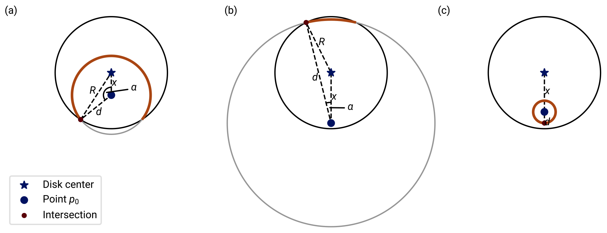
Figure E1 Geometry for the computation of the neighbor density by distance on a disk of radius R with uniform point density. This sketch illustrates the sets of points at a distance d from a test point on the disk. (a) For a point that is located at distance x from the disk center, the set of points at distance d within the disk is a circular segment that spans an angular range of 2α. This angle α is determined from the trigonometry of the parameters x, d, and R. (b) As the distance d approaches its upper limit 2R, the circular segment converges to a point that is antipodal to a point on the disk's perimeter (x=R). (c) If $x+d\le R$, the set of points at distance d from the test point is a full circle of radius d.

In this section, we derive the neighbor density of points drawn from a disk of radius R with uniform point density. This neighbor density is the probability density of the distance d between two points which are both drawn from a uniform point density on the disk. In other words, this distribution describes the following: if we draw two random points from the uniform density on the disk, what distance d do we expect between the two points?

Suppose that we have a point p₀ drawn randomly from the uniform distribution on the disk. Without loss of generality, we can rotate the disk as indicated in Fig. E1a so that p₀ is at distance x from the center of the disk. For the random point p₀ drawn from the disk, x follows the distribution

$$\begin{array}{}\text{(E1)}& p\left(x\right)={\displaystyle \frac{\mathrm{2}x}{R^{\mathrm{2}}}}.\end{array}$$

The orange circle wedge shows the set of points within the disk that are located at distance d from p₀. For the configuration shown in Fig. E1a, the wedge intersects the disk's border at the red dot. This dot can be parameterized by the angle α, measured counterclockwise from the line that connects p₀ with the disk's center. The angle can be computed by the law of cosines:

$$\begin{array}{}\text{(E2)}& \mathit{\alpha }(d,x,R)=\arccos \left({\displaystyle \frac{x^{\mathrm{2}}+d^{\mathrm{2}}-R^{\mathrm{2}}}{\mathrm{2}xd}}\right).\end{array}$$

The sketch of Fig. E1a equips us to compute the density of points at distance d from p₀ within the set of all points in the disk. Conceptually, we expand the light-gray circle from panel a from a point (d=0) up to the maximum size that intersects with the disk ($d=R+x$, indicated in panel b). For each d, the density is the length of the orange wedge, that is, 2αd, divided by the disk's area. If d is too large ($d>R+x$), the density is 0, and if $d\le R-x$, the length is the full circle perimeter (see Fig. E1c). The density of d conditional on x is hence

$$\begin{array}{}\text{(E3)}& p\left(d\right|x)\sim \left\{\begin{array}{ll}\mathrm{0}& :d>R+x\\ \mathrm{2}\mathit{\alpha }(d,x,R)d& :R-x<d\le R+x\\ \mathrm{2}\mathit{\pi }d& :d\le R-x\end{array}\right..\end{array}$$

To obtain the distance distribution within the population of pairs (p₀,p₁), this density needs to be averaged over the density p(x) of Eq. (E1). We hence find the density

$$\begin{array}{}\text{(E4)}& f\left(d\right)={\displaystyle \frac{\mathrm{1}}{F}}\underset{\mathrm{0}}{\overset{R}{\int }}\mathrm{d}xp\left(d\right|x\left)p\right(x)d\end{array}$$

with p(x) given in Eq. (E1), p(d | x) given in Eq. (E3), and with the normalization constant

$$\begin{array}{}\text{(E5)}& {\displaystyle }F=\underset{\mathrm{0}}{\overset{\mathrm{2}R}{\int }}\mathrm{d}y\underset{\mathrm{0}}{\overset{R}{\int }}\mathrm{d}xp\left(d\right|x\left)p\right(x)y.\end{array}$$

The resulting density is shown by dashed lines in Fig. 3. As d_min increases in that figure, the density of Eq. (E4) is adjusted by setting the lower y integration bound for F in Eq. (E5) to d_min.

Appendix F: Artificial surface heat flow with gamma-like aggregate distribution

This section describes how the artificial heat flow field in Fig. 2 is generated. The generation follows a two-step procedure.

First, a target surface heat flow distribution is generated on the x interval shown in Fig. 2a. This target heat flow distribution is determined through 13 equidistantly distributed points on the x range (the control points). On the two boundary points, the heat flow is set to 42 mW m⁻² (an arbitrary value within the range of heat flow encountered within regional samples of the NGHF; Lucazeau, 2019). The 11 remaining points are allowed to vary freely between 35 mW m⁻² and 50 mW m⁻². Between these 13 points, the heat flow field is interpolated using SciPy's smoothing cubic spline with a smoothing parameter of s=2 (Dierckx, 1975; Virtanen et al., 2020). The interpolated heat flow field is evaluated at 573 equidistant points on the x interval, and a cost function is constructed by computing the Anderson–Darling statistic for a maximum likelihood estimate of the gamma distribution on these 573 sample values. This cost is minimized by optimizing the heat flow values at the 11 control points using the SciPy implementation of the limited-memory bound-constrained Broyden–Fletcher–Goldfarb–Shanno (BFGS) optimizer (Byrd et al., 1996; Virtanen et al., 2020).

Once this target heat flow distribution with gamma-like aggregate distribution has been created, it is used as an optimization target for the heat flow generated by underground heat sources. Below the x extent shown in Fig. 2, x ∈ [−50 km, 75 km], a 200 km wide and 80 km deep grid is created with x ∈ [−80 km, 120 km] and 201×151 cells. The heat generation in each cell is allowed to vary between 0 W m⁻³ and 8 W m⁻³, below which most rock samples are found (Jaupart and Mareschal, 2005, Fig. 1). The material is assumed homogeneous with a thermal conductivity of 2.5 W m⁻¹ K⁻¹ (as used in Lachenbruch and Sass, 1980). At the surface, a temperature of 0 K is assumed. At 80 km depth, a boundary temperature of 318 K is enforced, causing a surface heat flow of 10 mW m⁻² that is superposed by any heat sources in the grid. The heat equation is solved on the grid using the finite difference method. Starting from a uniform heat generation of 0.8 W m⁻³ in each grid cell, the constrained trust-region optimization algorithm of SciPy (Conn et al., 2000; Virtanen et al., 2020) is used to minimize the squared deviations of the solved surface heat flow from the target heat flow evaluated at the corresponding surface points.

The code to generate Fig. 2 is part of the REHEATFUNQ model (Ziebarth, 2023, A9-Simple-Heat-Conduction.ipynb).

Appendix G: A note on nonlinear heat transport

This is a technical note on the applicability of REHEATFUNQ for nonlinear heat transport, brought to our attention by anonymous reviewer 1. A central equation for connecting the Bayesian methods with the physical model of heat conduction, ultimately leading to the P_H posterior distribution, is Eq. (18):

$$\begin{array}{}\text{(G1)}& {\displaystyle }{q}_{\mathrm{a}}\left({\mathit{x}}_i\right)=P_{\mathrm{H}}c\left({\mathit{x}}_i\right).\end{array}$$

This equation assumes linearity of the heat conduction in heat power P_H – which is the case for heat conduction if P_H is sufficiently small but may break down as other means of heat transport set in as P_H increases. In such a case of nonlinear heat transport, the anomaly may in general be of the non-decomposable form

$$\begin{array}{}\text{(G2)}& {\displaystyle }{q}_{\mathrm{a}}\left({\mathit{x}}_i\right)=\mathfrak{q}(P_{\mathrm{H}},{\mathit{x}}_i).\end{array}$$

REHEATFUNQ is not able to handle such non-decomposable nonlinearities in heat transport. The linear decomposition of q_a(x_i) into a constant coefficient c_i and a variable but global magnitude parameter (here P_H) is required. However, there is one kind of nonlinear dependence of the heat transport onto the power P_H that fulfills this requirement: a factorization into a function of P_H and a function of x,

$$\begin{array}{}\text{(G3)}& {\displaystyle }{q}_{\mathrm{a}}\left({\mathit{x}}_i\right)=\mathfrak{p}\left(P_{\mathrm{H}}\right)\mathfrak{c}\left({\mathit{x}}_i\right).\end{array}$$

With this, one could simply provide {𝔠(x_i)} instead of {c_i} to REHEATFUNQ. The posterior PDF f and CDF F would then be evaluated in 𝔭 instead of the heat power P_H. This result would then have to be manually transformed to P_H by inverting the function 𝔭(P_H).

We do not know whether there are cases of nonlinear heat transport that factorize according to Eq. (G3) and show no spatial nonlinearity and hence whether this note is relevant. We leave this open for further study.